The Markov Chain Monte Carlo Revolution

Persi Diaconis∗

Abstract

The use of simulation for high dimensional intractable computations has revolutionized applied math-ematics. Designing, improving and understanding the new tools leads to (and leans on) fascinatingmathematics, from representation theory through micro-local analysis.

1 Introduction

Many basic scientific problems are now routinely solved by simulation: a fancy “random walk” is performedon the system of interest. Averages computed from the walk give useful answers to formerly intractableproblems. Here is an example drawn from course work of Stanford students Marc Coram and Phil Beineke.

Example 1 (Cryptography). Stanford’s Statistics Department has a drop-in consulting service. One day,a psychologist from the state prison system showed up with a collection of coded messages. Figure 1 showspart of a typical example.

Figure 1

The problem was to decode these messages. Marc guessed that the code was a simple substitution cipher,each symbol standing for a letter, number, punctuation mark or space. Thus, there is an unknown functionf

f : code space −→ usual alphabet.One standard approach to decrypting is to use the statistics of written English to guess at probable choicesfor f , try these out, and see if the decrypted messages make sense.

To get the statistics, Marc downloaded a standard text (e.g., War and Peace) and recorded the first-order transitions: the proportion of consecutive text symbols from x to y. This gives a matrix M(x, y) oftransitions. One may then associate a plausibility to f via

Pl(f) =∏i

M (f(si), f(si+1))

∗Departments of Mathematics and Statistics, Stanford University

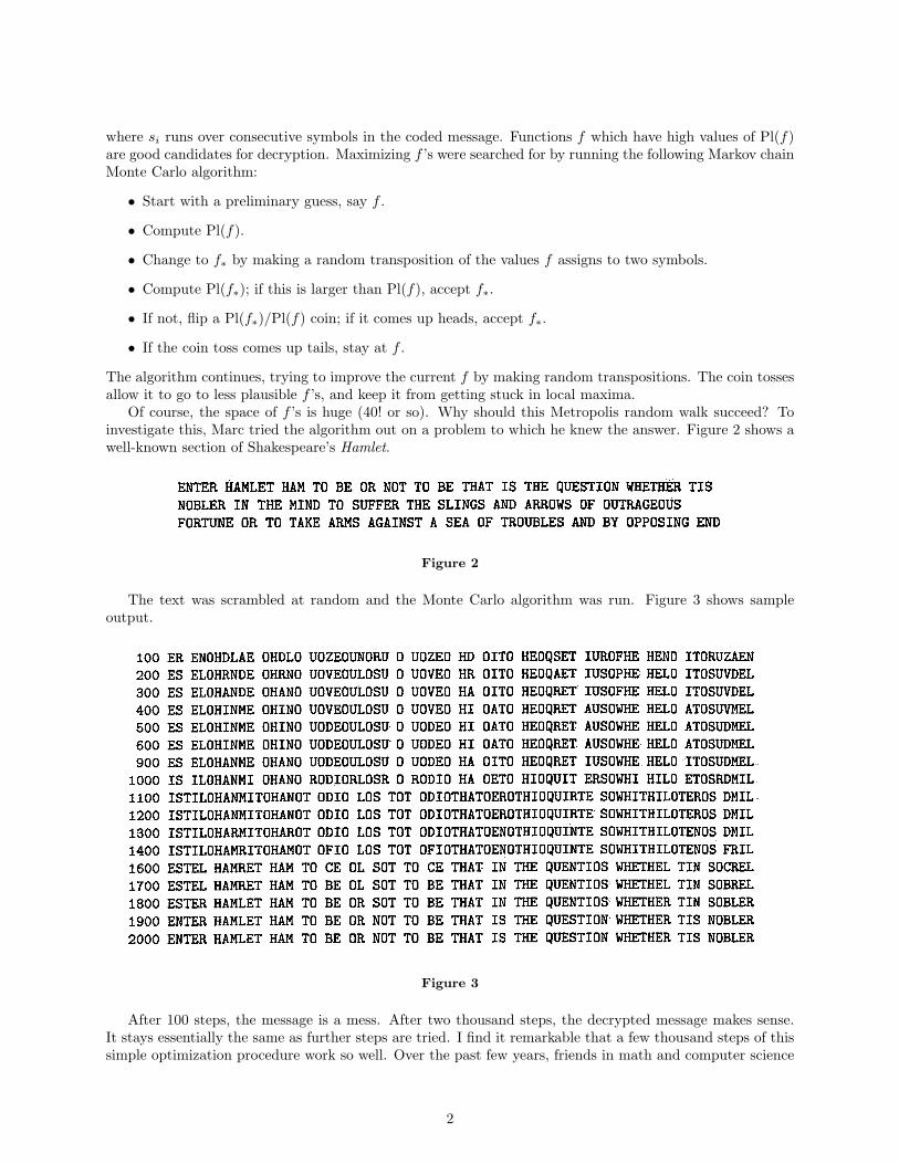
where si runs over consecutive symbols in the coded message. Functions f which have high values of Pl(f)are good candidates for decryption. Maximizing f ’s were searched for by running the following Markov chainMonte Carlo algorithm:

• Start with a preliminary guess, say f .

• Compute Pl(f).

• Change to f∗ by making a random transposition of the values f assigns to two symbols.

• Compute Pl(f∗); if this is larger than Pl(f), accept f∗.

• If not, flip a Pl(f∗)/Pl(f) coin; if it comes up heads, accept f∗.

• If the coin toss comes up tails, stay at f .

The algorithm continues, trying to improve the current f by making random transpositions. The coin tossesallow it to go to less plausible f ’s, and keep it from getting stuck in local maxima.

Of course, the space of f ’s is huge (40! or so). Why should this Metropolis random walk succeed? Toinvestigate this, Marc tried the algorithm out on a problem to which he knew the answer. Figure 2 shows awell-known section of Shakespeare’s Hamlet.

Figure 2

The text was scrambled at random and the Monte Carlo algorithm was run. Figure 3 shows sampleoutput.

Figure 3

After 100 steps, the message is a mess. After two thousand steps, the decrypted message makes sense.It stays essentially the same as further steps are tried. I find it remarkable that a few thousand steps of thissimple optimization procedure work so well. Over the past few years, friends in math and computer science

2

courses have designed homework problems around this example [17]. Students are usually able to successfullydecrypt messages from fairly short texts; in the prison example, about a page of code was available.

The algorithm was run on the prison text. A portion of the final result is shown in Figure 4. It gives auseful decoding that seemed to work on additional texts.

Figure 4

I like this example because a) it is real, b) there is no question the algorithm found the correct answer,and c) the procedure works despite the implausible underlying assumptions. In fact, the message is in a mixof English, Spanish and prison jargon. The plausibility measure is based on first-order transitions only. Apreliminary attempt with single-letter frequencies failed. To be honest, several practical details have beenomitted: we allowed an unspecified “?” symbol in the deviation (with transitions to and from “?” beinginitially uniform). The display in Figure 4 was ‘cleaned up’ by a bit of human tinkering. I must also add thatthe algorithm described has a perfectly natural derivation as Bayesian statistics. The decoding function f isa parameter in a model specifying the message as the output of a Markov chain with known transition matrixM(x, y). With a uniform prior on f , the plausibility function is proportional to the posterior distribution.The algorithm is finding the mode of the posterior.

In the rest of this article, I explain Markov chains and the Metropolis algorithm more carefully inSection 2. A closely related Markov chain on permutations is analyzed in Section 3. The arguments usesymmetric function theory, a bridge between combinatorics and representation theory.

A very different example — hard discs in a box — is introduced in Section 4. The tools needed for studyare drawn from analysis, micro-local techniques (Section 5) along with functional inequalities (Nash andSobolev inequalities).

Throughout, emphasis is on analysis of iterates of self-adjoint operators using the spectrum. Thereare many other techniques used in modern probability. A brief overview, together with pointers on how abeginner can learn more, is in Section 6.

2 A Brief Treatise on Markov Chains

2.1 A finite case

Let X be a finite set. A Markov chain is defined by a matrix K(x, y) with K(x, y) ≥ 0,∑yK(x, y) = 1

for each x. Thus each row is a probability measure so K can direct a kind of random walk: from x, choosey with probability K(x, y); from y choose z with probability K(y, z), and so on. We refer to the outcomesX0 = x,X1 = y,X2 = z, . . . as a run of the chain starting at x. From the definitions P (X1 = y|X0 = x) =K(x, y), P (X1 = y,X2 = z|X0 = x) = K(x, y)K(y, z). From this, P (X2 = z|X0 = x) =

∑yK(x, y)K(y, z),

and so on. The nth power of the matrix has x, y entry P (Xn = y|X0 = x).

3

All of the Markov chains considered in this article have stationary distributions π(x) > 0,∑x π(x) = 1

with π satisfying ∑x

π(x)K(x, y) = π(y). (2.1)

Thus π is a left eigenvector of K with eigenvalue 1. The probabilistic interpretation of (2.1) is “pick x fromπ and take a step from K(x, y); the chance of being at y is π(y).” Thus π is stationary for the evolution.The fundamental theorem of Markov chains (a simple corollary of the Peron–Frobenius theorem) says, undera simple connectedness condition, π is unique and high powers of K converge to the rank one matrix withall rows equal to π.

Theorem 1 (Fundamental Theorem of Markov Chains). Let X be a finite set and K(x, y) a Markov chainindexed by X . If there is n0 so that Kn(x, y) ≥ 0 for all n > n0, then K has a unique stationary distributionπ and, as n→∞,

Kn(x, y)→ π(y) for each x, y ∈ X .

The probabilistic content of the theorem is that from any starting state x, the nth step of a run of theMarkov chain has chance close to π(y) of being at y if n is large. In computational settings, |X | is large, itis easy to move from x to y according to K(x, y) and it is hard to sample from π directly.

Consider the cryptography example in the introduction. There, X is the set of all 1–1 functions f fromcode space to the usual alphabet A,B, . . . ,Z, 1, 2, . . . , 9, 0, ∗, ., ?, . . . . Assume there are m distinct codesymbols and n symbols in the alphabet space. The stationary distribution is

π(f) = z−1∏i

M (f(si), f(si+1)) (2.2)

where M is the (assumed given) first-order transition matrix of English and the product ranges over consec-utive coded symbols in the fixed message. The normalizing constant z is defined by

z =∑f

∏i

(M (f(si), f(si+1))) .

Note that z is unknowable practically.The problem considered here is to sample f ’s repeatedly from π(f). This seems daunting because of the

huge size of X and the problem of unknown z. The Metropolis Markov chain K(f, f∗) solves this problem.

2.2 Metropolis algorithm

Let X be a finite state space and π(x) a probability on X (perhaps specified only up to an unknownnormalizing constant). Let J(x, y) be a Markov matrix on X with J(x, y) > 0↔ J(y, x) > 0. At the start,J is unrelated to π. The Metropolis algorithm changes J to a new Markov matrix K(x, y) with stationarydistribution π. It is given by a simple recipe:

K(x, y) =

J(x, y) if x 6= y, A(x, y) ≥ 1J(x, y)A(x, y) if x 6= y, A(x, y) < 1

J(x, y) +∑

z:A(x,z)<1

J(x, z)(1−A(x, z)) if x = y. (2.3)

In (2.3), the acceptance ratio is A(x, y) = π(y)J(y, x)/π(x)J(x, y). The formula (2.3) has a simple interpre-tation: from x, choose y with probability J(x, y); if A(x, y) ≥ 1, move to y; if A(x, y) < 1, flip a coin withthis success probability and move to y if success occurs; in other cases, stay at x. Note that the normalizingconstant for π cancels out in all calculations. The new chain satisfies

π(x)K(x, y) = π(y)K(y, x)

and thus ∑x

π(x)K(x, y) =∑x

π(y)K(y, x) = π(y)∑x

K(y, x) = π(y),

4

so that π is a left eigenvector with eigenvalue 1. If the chain (2.3) is connected, Theorem 1 is in force. Aftermany steps of the chain, the chance of being at y is approximately π(y), no matter what the starting stateX . Textbook treatments of the Metropolis algorithm are in [44] or [62]. A literature review can be found in[31].

In the cryptography example X is all 1–1 functions from symbol space (say of size m) to alphabet space(say of size n ≥ m). Thus |X | = n(n− 1) . . . (n−m+ 1). This is large if, e.g., m = n = 50. The stationarydistribution is given in (2.2). The proposal chain J(f, f∗) is specified by a random switch of two symbols,

J(f, f∗) =

1

n(n−1)(m−n+2)(m−n+1) if f, f∗ differ in at most two places

0 otherwise.

Note that J(f, f∗) = J(f∗, f) so A(f, f∗) = π(f∗)/π(f).

2.3 Convergence

A basic problem of Markov chain theory concerns the rate of convergence in Kn(x, y)→ π(y). How long mustthe chain be run to be suitably close to π? It is customary to measure distances between two probabilitiesby total variation distance

‖Knx − π‖TV =

12

∑y

|Kn(x, y)− π(y)| = maxA⊆X

|Kn(x,A)− π(A)|.

This yields the math problem: Given K,π, x and ε > 0, how large n so

‖Knx − π‖TV < ε?

Sadly, there are very few practical problems where this question can be answered. In particular, no usefulanswer in known for the cryptography problem. In Section 3, a surrogate problem is set up and solved. Itsuggests that when n

.= m, order n log n steps suffice for mixing.Suppose, as is the case for the examples in this paper, that the Markov chain is reversible: π(x)K(x, y) =

π(y)K(y, x). Let L2(π) be g : X → R with inner product 〈g, h〉 =∑x g(x)h(x)π(x). Then K operates

on L2 by Kg(x) =∑g(y)K(x, y). Reversibility implies 〈Kg, h〉 = 〈g,Kh〉, so K is self-adjoint. Now, the

spectral theorem says there is an orthonormal basis of eigenvectors ψi and eigenvalues βi (so Kψi = βiψi)for 0 ≤ i ≤ |X | − 1 and 1 = β0 ≥ β1 ≥ · · · ≥ β|X |−1 ≥ −1. By elementary manipulations

K(x, y) = π(y)|X |−1∑i=0

βiψi(x)ψi(y), Kn(x, y) = π(y)|X |−1∑i=0

βni ψi(x)ψi(y).

Using the Cauchy–Schwartz inequality, we have

4‖Knx − π‖2TV ≤

∑y

(Kn(x, y)− π(y))2

π(y)=|X |−1∑i=1

β2ni ψ2

i (x). (2.4)

The bound (2.4) is the basic eigenvalue bound used to get rates of convergence for the examples presentedhere. To get sharp bounds on the right hand side requires good control of both eigenvalues and eigenvectors.For more details and many examples, see [79]. A detailed example on the permutation group is given inSection 3 below. Examples on countable and continuous spaces are given in Section 5.

2.4 General state spaces

Markov chains are used to do similar calculations on Euclidean and infinite-dimensional spaces. My favoriteintroduction to Markov chains is the book by Bremaud [10], but there are many sources; for finite statespaces see [83]. For a more general discussion, see [7] and the references in Section 6.1.

5

Briefly if (X , B) is a measurable space, a Markov kernel K(x, dy) is a probability measure K(x, ·) foreach x. Iterates of the kernel are given by, e.g.,

K2(x,A) =∫K(z,A)K(x, dz).

A stationary distribution is a probability π(dx) satisfying

π(A) =∫K(x,A)π(dx)

under simple conditions Kn(x,A)→ π(A) and exactly the same problems arise.Reversible Markov chains yield bounded self-adjoint operators and spectral techniques can again be tried.

Examples are in Section 4, Section 5, and Section 6.

3 From Cryptography to Symmetric Function Theory

This section answers the question, “What does a theorem in this subject look like?” It also illustrates howeven seemingly simple problems can call on tools from disparate fields: here, symmetric function theory, ablend of combinatorics and representation theory. This section is drawn from joint work with Phil Hanlon[21].

3.1 The problem

Let X = Sn, the symmetric group on n letters. Define a probability measure on Sn by

π(σ) = z−1θd(σ,σ0) for σ, σ0 ∈ Sn, 0 < θ ≤ 1. (3.1)

In (3.1), d(σ, σ0) is a metric on the symmetric group, here taken to be

d(σ, σ0) = minimum number of transpositions required to bring σ to σ0.

This is called Cayley’s distance in [20] because a result of A. Cayley implies that d(σ, σ0) = n − c(σ−1σ0)with c(σ) the number of cycles in σ. The metric is bi-invariant: d(σ, σ0) = d(τσ, τσ0) = d(στ, σ0τ). Thenormalizing constant z is known in this example: z =

∑σ θ

d(σ,σ0) =∏ni=1(1 + θ(i− 1)).

If θ = 1, π(σ) is the uniform distribution on Sn. For θ < 1, π(σ) is largest at σ0 and falls off from itsmaximum as σ moves away from σ0. It serves as a natural non-uniform distribution on Sn, peaked at apoint. Further discussion of this construction (called Mallows model through Cayley’s metric) with examplesfrom psychology and computer science is in [18, 19, 28]. The problem studied here is

How can samples be drawn from σ?

One route is to use the Metropolis algorithm, based on random transpositions. Thus, from σ, choose atransposition (i, j) uniformly at random and consider (i, j)σ = σ∗. If d(σ∗, σ0) ≤ d(σ, σ0) the chain movesto σ∗. If d(σ∗, σ0) > d(σ, σ0), flip a θ-coin. If this comes up heads, move to σ∗; else stay at σ. In symbols,

K(σ, σ∗) =

1/(n2

)if σ∗ = (i, j)σ, d(σ∗, σ0) < d(σ, σ0)

θ/(n2

)if σ∗ = (i, j)σ, d(σ∗, σ0) > d(σ, σ0)

c(1− θ/

(n2

))if σ∗ = σ, with c = # (i, j) : d((i, j)σ, σ0) > d(σ, σ0)

0 otherwise.

(3.2)

Observe that this Markov chain is “easy to run.” The Metropolis construction guarantees that:

π(σ)K(σ, σ∗) = π(σ∗)K(σ∗, σ)

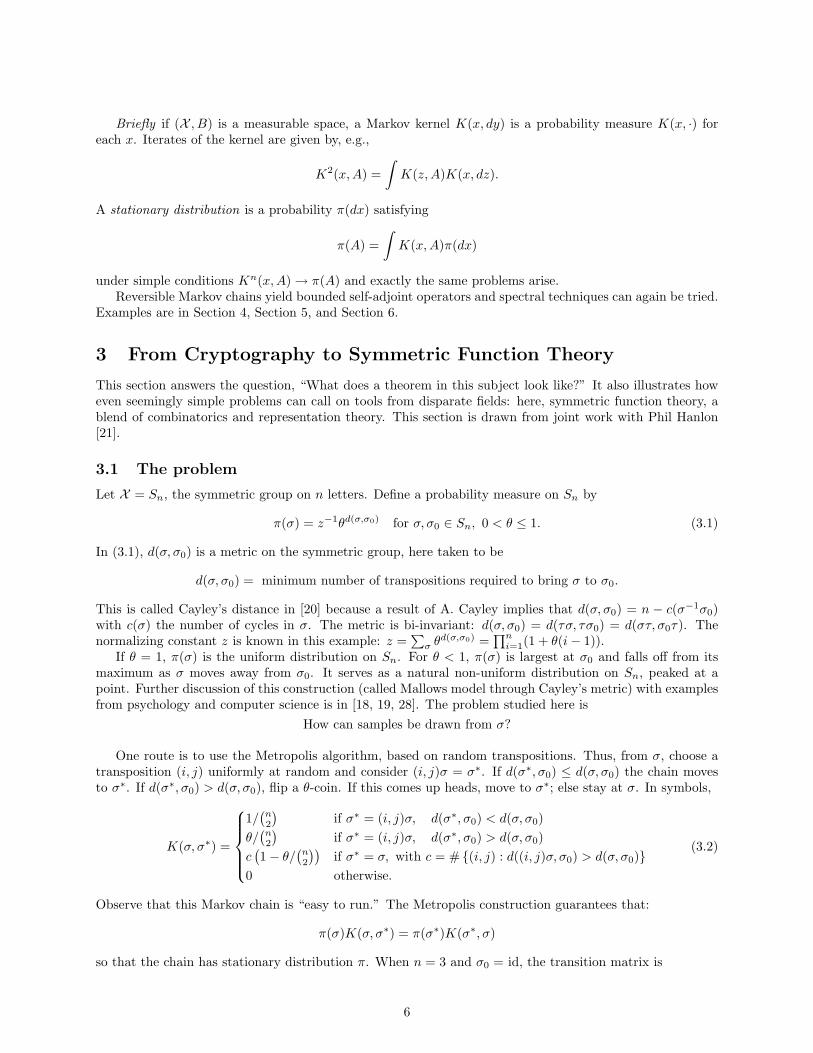
so that the chain has stationary distribution π. When n = 3 and σ0 = id, the transition matrix is

6

id (12) (13) (23) (123) (132)id

1− θ θ3

θ3

θ3 0 0

13

23 (1− θ) 0 0 θ

3θ3

13 0 2

3 (1− θ) 0 θ3

θ3

13 0 0 2

3 (1− θ) θ3

θ3

0 13

13

13 0 0

0 13

13

13 0 0

(12)(13)(23)(123)(132)

The stationary distribution is the left eigenvector proportional to (1, θ, θ, θ, θ2, θ2).

This example bears a passing resemblance to the cryptography example: the set of 1 − 1 functions ofan m-set to an n-set is replaced by the symmetric group. Presumably, the stationary distribution in thecryptography example is peaked at a point (the best decoding) and the algorithms are essentially the same.

To analyze the chain (3.2) using spectral theory requires knowledge of the eigenvalues and vectors. Bywhat still seems like a miracle, these are available in closed form. When θ = 1, the chain (3.2) reduces to the‘transpose at random chain’, perhaps the first Markov chain given a sharp analysis [32]. Here is a typicalresult.

Theorem 2. For 0 < θ ≤ 1, the Markov chain K(σ, σ∗) in (3.2) has stationary distribution π from (3.1).Let k = an log n + cn with a = 1/2θ + 1/4θ(1/θ − θ) and c > 0. Then, with σ0 = id and starting from theidentity

‖Kk − π‖TV ≤ f(θ, c)

with f(θ, c)→ 0 for c→ 0.

Remarks. The result shows that order n log n steps suffice to make the distance to stationarity small. Thefunction f(θ, c) is explicit but a bit of a mess. There is a matching lower bound showing that order n log nsteps are necessary as well. In the theorem, σ0 was chosen as the identity and the chain starts at σ0. If thechain starts far from the identity, for example at an n-cycle, it can be shown that order n2 log n steps suffice.When, e.g., n = 52, n log n .= 200 while n2 log n .= 11, 000. These numbers give a useful feel for the runningtime.

3.2 Tools from symmetric function theory

The first step of analysis is to reduce the state space from the full symmetric group to the set of conjugacyclasses. (Recall these are indexed by partitions of n.) The matrix K(σ, σ∗) commutes with the action of thesymmetric group by conjugation, so only transitions between conjugacy classes are needed. When n = 3 thetransition matrix becomes

13 1, 2 313

1− θ θ 013

23 (1− θ) 2

3θ

0 1 0

1, 23

with stationary distribution proportional to (1, 3θ, 2θ2). Let

M(µ, λ), m(λ) (3.3)

be the transition matrix and stationary distribution indexed by partitions λ, µ.

Theorem 3. For 0 < θ ≤ 1, the Markov chain (3.3) has an eigenvalue βλ for each partition (λ1, λ2, . . . , λr)of n with

βλ = (1− θ) +θn(λt) + n(λ)(

n2

) , n(λ) =n∑i=1

(i− 1)λi.

7

The corresponding right eigenfunction, normed to be orthonormal in L2(m), is

cλ(·)m(λ)jλπ/θnn!1/2

. (3.4)

In (3.4), cλ are the change of basis coefficients in expressing the Jack symmetric functions in terms of thepower-symmetric functions. The normalizing constant in (3.4) involves closed form, combinatorially-definedterms which will not be detailed further.

Here is an aside on the cλ(·). Classical combinatorics involves things like partitions, permutations, graphs,balls in boxes and so on. A lot of this has been unified and extended in the subject of algebraic combinatorics.A central theme here is the ring Λn(x1 . . . xk) of homogeneous symmetric polynomials of degree n. There arevarious bases for this space. For example, if Pi(x1 . . . xk) =

∑xij and Pλ = Pλ1Pλ2 . . . Pλn , the Pλ form a

basis as λ runs through the partitions of n (fundamental theorem of symmetric functions). Other well-knownbases are the monomial and elementary symmetric functions. The stars of the show are the Schur functions(character of the general linear group). The change of basis matrices between these codes up a lot of classicalcombinatorics. A two-parameter family of bases, the Macdonald polynomials, is a central focus of moderncombinatorics. Definitive, inspiring accounts of this are in Macdonald [65] and Stanley [82].

The Jack symmetric functions Jλ(x;α) is one of the many bases. Here x = (x1 . . . xk) and α is a positivereal parameter. When α = 1, the Jacks become the Schur functions. When α = 2, the Jacks become thezonal polynomials (spherical functions of GLn/On). Before the work with Hanlon, no natural use for othervalues of α was known. Denote the change of basis coefficients from Jacks to power sums by

Jλ(x;α) =∑µ`n

c(λ, µ)Pµ(x).

The c(λ, µ) are rational functions of α. For example, when n = 3,

J13 = P 31 − 3P12 − 2P3

J12 = P 31 + (α− 1)P12 − αP3

J3 = P 31 − 3αP12 + 2α2P3

The algebraic combinatorics community had developed properties of Jack symmetric functions “because theywere there.” Using this knowledge allowed us to properly normalize the eigenfunctions and work with themto prove Theorems 1 and 2. Many more examples of this type of interplay are in [14]. A textbook accountof our work is in [48].

There is a fascinating research problem opened up by this analysis. When θ = 1, the Jack symmetricfunctions are Schur functions and the change of basis coefficients are the characters of the symmetric group.The Markov chain becomes ‘random transpositions’. This was analyzed in joint work with Shahshahani[32]. Adding in the deformation by the Metropolis algorithm deforms the eigenvalues and eigenvectors ina mathematically natural way. Is there a similar deformation that gets the coefficients of the Macdonaldpolynomials? This is ongoing joint work with Arun Ram. Changing the metric on Sn, using pairwise adjacenttranspositions instead of all transpositions, gives a deformation to Hecke algebras. The Metropolis algorithmgives a probabilistic interpretation of the multiplication in these algebras. This again is joint work with Ram[28]. This affinity between the physically natural Metropolis algorithm and algebra is a mystery which criesout for explanation.

Turning back toward the cryptography example, how do things change if we go from the permutationgroup to the set of 1− 1 functions from an m-set to an n-set? When θ = 1, this was worked out by AndrewGreenhalgh. The analysis involves the algebra of functions on Sn which are invariant under conjugation bythe subgroup Sm × Sn−m and bi-invariant under the subgroup Sn−m. These “doubly invariant functions”form a commutative algebra discussed further in Ceccherini-Silberstein et al. [14], Sect. 9.8. Do things deformwell when θ 6= 1? It is natural to guess the answer is Yes.

It is important to end these fascinating success stories with the observation that any similarly usefulanalysis of the original cryptography example seems remote. Further, getting rates of convergence for theMetropolis algorithm for other metrics in (3.1) is a challenging open problem.

8

4 Hard Discs in a Box

Consider possible placements of n discs of radius ε in the unit square. The discs must be non-overlappingand completely contained in the unit square. Examples at low and high density (kindly provided by WernerKrauth from [57]) are shown in Figure 5.

! = 0.48(a) Low density

! = 0.72(b) High density

Figure 5

In applications, n is fairly large (e.g., 100–106) and of course ε should be suitably small. The centers of thediscs give a point in R2n. We know very, very little about the topology of the set X (n, ε) of configurations:for fixed n, what are useful bounds on ε for the space to be connected? What are the Betti numbers? Ofcourse, for ε “small” this set is connected but very little else is known. By its embedding in R2n, X (n, ε)inherits a natural uniform distribution, Lebesgue measure restricted to X (n, ε). The problem is to pickpoints in X (n, ε) uniformly. If X1, X2, . . . , Xk are chosen from the uniform distribution and f : X (n, ε)→ Ris a function, we may approximate ∫

X (n,ε)

f(x)dx by1k

k∑i=1

f(Xi). (4.1)

Motivation for this task and some functions f of interest will be given at the end of this section.This hard discs problem is the original motivation for the Metropolis algorithm. Here is a version of the

Metropolis algorithm for hard discs.

• Start with some x ∈ X (n, ε).

• Pick a disc center at random (probability 1/n).

• Pick a point in a disc of radius h, centered at the chosen disc center at random (from Lebesgue measure).

• Try to move the chosen disc center to the chosen point; if the resulting configuration is in X (n, ε),accept the move; else, stay at x.

The algorithm continues, randomly moving coordinates. If X1, X2, . . . , Xk denotes the successive configura-tions, theory shows that Xk becomes uniformly distributed provided ε, k are small. For large k, the Xi canbe used as in (4.1).

Motivation

The original motivation for this problem comes from the study of phase transition in statistical mechanics.For many substances (e.g., water), experiments produce phase diagrams such as that shown in Figure 6.Every aspect of such phase diagrams is intensely studied. The general picture, a finite length liquid–vaporphase transition line ending in a critical point, a triple point where all three forms co-exist and a solid–liquidphase line seemingly extending to infinity, seems universal. The physicist G. Uhlenbeck [87, p. 11] writes“Note that since these are general phenomena, they must have general explanation; the precise details ofthe molecular structure and of the intermolecular forces should not matter.” In discussing the solid–liquid

9

Figure 6

transition, Uhlenbeck (p. 18) notes that the solid–liquid transition seemingly occurs at any temperatureprovided the pressure is high enough. He suggests that at high pressure, the attractive intermolecular forcedoes not play a role “. . . and that it is the sharp repulsive forces that are responsible for the solid–fluidtransition. It is this train of thought which explains the great interest of the so-called Kirkwood transition.In 1941, Kirkwood posed the problem of whether a gas of hard spheres would show a phase transition. . . .”

From then to now, chemists and physicists have studied this problem using a variety of tools. Currentfindings indicate a phase transition when the density of discs is large (about .71, still well below the closepacking density). Below this transition density, the discs “look random”; above this density the discs lookclose to a lattice packing. These notions are quantified by a variety of functions f . For example

f(x) =

∣∣∣∣∣∣ 1N

N∑j=1

1Nj

∑k

e6iθjk

∣∣∣∣∣∣where the sum is over the N particles encoded by x ∈ R2N , the sum in k is over the Nj neighbors of the jthparticle and θjk is the angle between the particles j and k in an arbitrary but fixed reference frame. If theconfiguration x has a local hexatic structure, this sum should be small. Typical values of f are studied bysimulation. Different functions are used to study long-range order.

The above rough description may be supplemented by the useful survey of [64]. A host of simulationmethods are detailed in [2]. An up-to-date tutorial on hard discs appears in [57, Chap. 2].

For purposes of this paper, the main points are i) the hard disc model is a basic object of study and ii)many key findings have been based on variants of the Metropolis algorithm. In the next section, we flushout the Metropolis algorithm to more standard mathematics.

5 Some Mathematics

Here is a generalization of the hard discs Metropolis algorithm. Let Ω ⊆ Rd be a bounded connected openset. Let p(x) > 0, z =

∫Ωp(x)dx <∞, p(x) = z−1p(x) specify a probability density on Ω. If required, extend

p to have value 0 outside the closure of Ω. Many sampling problems can be stated thus:

Given p, choose points in Ω from p.

Note that the normalizing constant z may not be given and is usually impossible to usefully approximate.As an example, consider placing fifty hard discs in the unit square when ε = 1/100. The set of allowableconfigurations is a complex, cuspy set. While p ≡ 1 on Ω, it would not be practical to compute z. Here isone version of the Metropolis algorithm which samples from p. From x ∈ Ω, fix a small, positive h.

• Choose y ∈ Bx(h), from normalized Lebesgue measure on this ball.

• If p(y) ≥ p(x), move to y.

• If p(y) < p(x), move to y with probability p(y)/p(x).

• Else stay at x.

10

Note that this algorithm does not require knowing z. The transition from x to y yields a transition kernel

P (x, dy) =m(x)δx +h−d

Vol(B1)δB1

(x− yh

)min

(p(x)p(y)

, 1)dy

with m(x) = 1−∫

Rd

h−d

Vol(B1)δB1

(x− yh

)min

(p(x)p(y)

, 1)dy.

(5.1)

This kernel operates on L2(p) via

P · f(x) =∫

Rdf(y)P (x, dy).

It is easy to see that P (x, dy) is a bounded self-adjoint operator on L2(p). The associated Markov chainmay be described ‘in English’ by

• Start at X0 = x ∈ Ω.

• Pick X1 from P (x, dy).

• Pick X2 from P (X1, dy).

• And so on . . . .

Thus PX2 ∈ A = P 2x (A) =

∫Rd P (z,A)P (x, dz), PXk ∈ A = P kx (A) =

∫Rd P (z,A)P k−1(x, dz). Under

our assumptions (Ω connected, h small), for all x ∈ Ω and A ⊆ Ω, the algorithm works:

P kx (A) k−→∞

∫A

p(y)dy.

It is natural to ask how fast this convergence takes place: How many steps should the algorithm be run todo its job? In joint work with Gilles Lebeau and Laurent Michel, we prove the following.

Theorem 4. Let Ω be a connected Lipshitz domain in Rd. For p measurable (with 0 < m ≤ p(x) ≤M <∞on Ω) and h fixed and small, the Metropolis algorithm (5.1) satisfies∣∣∣∣P kx (A)−

∫A

p(y)dy∣∣∣∣ ≤ c1e−c2kh2

uniformly in x ∈ Ω, A ⊆ Ω. (5.2)

In (5.2), c1, c2 are positive constants that depend on p and Ω but not on x, k or h. The result is sharpin the sense that there is a matching lower bound. Good estimates of c2 are available (see the followingsection).

Note that the Metropolis algorithm (5.1) is based on steps in the full-dimensional ball Bε(x) while theMetropolis algorithm for discs in Section 2 is based on just changing two coordinates at a time. With extraeffort, a result like (5.2) can be shown for the hard disc problem as well. Details are in [25]. As a caveat,note that we do not have good control on c1 in terms of the dimension d or smoothness of Ω. The resultsare explicit but certainly not sharp.

The Metropolis algorithm of this section is on a Euclidean space with basic steps driven by a ‘ball walk.’None of this is particularly important. The underlying state space can be quite general, from finite (all 1−1functions from one finite set to another as in our cryptography example) to infinite-dimensional (Markovchains on spaces of measures). The proposal distribution needn’t be symmetric. All of the introductorybooks on simulation discussed in Section 6 develop the Metropolis algorithm. In [8] it is shown to bethe L1 projection of the proposal distribution to the p self-adjoint kernels on Ω. A survey of rates ofconvergence results on finite state spaces with extensive references to the work of computer science theoristson “approximate counting” and mathematical physicists on “Ising models” is in [31]. Finally, there are manyother classes of algorithms and proof techniques in active development. This is brought out in Section 6below.

11

5.1 Ideas and tools

To analyze rates of convergence it is natural to try spectral theory, especially if the operators are self-adjoint.This sometimes works. It is sometimes necessary to supplement with tools such as comparison and extensiontheory, Weyl-type bounds on eigenvalues, bounds on eigenvectors and Nash–Sobolev inequalities. These arebasic tools of modern analysis. Their use in a concrete problem may help some readers come into contactwith this part of the mathematical world.

Spectral bounds for Markov chains

Let X be a set, µ(dx) a reference measure and m(x) a probability density with respect to µ (so m(x) ≥0,∫m(x)µ(dx) = 1). Let P (x, dy) be a Markov kernel on X . This means that for each x, P (x, ·) is a

probability measure on X . This P may be used to “run a Markov chain” X0, X1, X2, . . . , with starting stateX0 = x say, by choosing X1 from P (x, ·) and then X2 from P (X1, ·), and so on. The pair (m,P ) is calledreversible (physicists say “satisfies detailed balance”) if P operating on L2(m) by Pf(x) =

∫f(y)P (x, dy)

is self-adjoint: 〈Pf, g〉 = 〈f, Pg〉. Often, P (x, dy) = p(x, y)µ(dy) has a kernel and reversibility becomesm(x)p(x, y) = m(y)p(y, x) for all x, y. This says the chain run forward is the same as the chain runbackward, in analogy with the time reversibility of the laws of mechanics. Here P operates on all of L2(m)so we are dealing with bounded self-adjoint operators.

Suppose for a moment that P has a square integrable kernel p(x, y), so Pf(x) =∫X p(x, y)f(y)µ(dy).

Then P is compact and there are eigenvectors fi and eigenvalues βi so

Pfi = βifi

under a mild connectedness condition f0 ≡ 1, β0 = 1 and 1 = β0 > β1 ≥ β2 ≥ · · · > −1. Then

p(x, y) = m(x)∞∑i=0

βifi(x)fi(y)

and the iterated kernel satisfies

pn(x, y) = m(y)∞∑i=0

βni fi(x)fi(y).

If fi(x), fi(y) are bounded (or at least controllable), since f0 ≡ 1,

pn(x, y)→ m(y) as n→∞.

This is the spectral approach to convergence. Note that to turn this into a quantitative bound (From startingstate x, how large must n be to have ‖Pnx −m‖ < ε?), the βi and fi must be well understood.

The Metropolis algorithm on the permutation group discussed in Section 3 gives an example on finitespaces. Here is an example with an infinite state space drawn from my work with Khare and Saloff-Coste[23] where this program can be usefully pushed through. Note that this example does not arise from theMetropolis construction. It arises from a second basic construction, Glauber dynamics.

Example 2 (Birth and Immigration). The state space X = 0, 1, 2, . . . . Let µ(dx) be counting measureand

m(x) =1

2x+1, p(x, y) =

(13

)x+y+1(x+ y

x

)/(12

)x+1

(5.3)

This Markov chain is used to model population dynamics with immigration. If the population size atgeneration n is denoted X then, given Xn = x,

Xn+1 =x∑i=1

Ni,n +Mn+1

where Ni,n, the number of offspring of the ith member of the population at time n, are assumed to beindependent and identically distributed with

p(Ni,n = j) =23

(13

)j, 0 ≤ j <∞.

12

Here Mn+1 is migration, assumed to have the same distribution as Ni,n. Note that m(x)p(x, y) = m(y)p(y, x)so reversibility is in force.

In (5.3) the eigenvalues are shown to be βj = 1/2j , 0 ≤ j < ∞. The eigenfunctions are the orthogonalpolynomials for the measure 1/2j+1. These are Meixner polynomials Mj(x) = 2F1

((−j−x1

)| − 1

). Now, the

spectral representation gives the following.

Proposition 1. For any starting state x for all n ≥ 0

χ2x(n) =

∞∑y=0

(pn(x, y)−m(y))2

m(y)=∞∑i=1

β2ni M2

i (x)12i.

Next, there is an analysis problem: Given the starting population x, how large should n be so that thischi-square distance to m is small? For this simple case, the details are easy enough to present in public.

Proposition 2. With notation as in Proposition 1,

χ2x(n) ≤ 2−2c for n = log2(1 + x) + c, c > 0

χ2x(n) ≥ 22c for n = log2(x− 1)− c, c > 0.

Proof. Meixner polynomials satisfy for all j and x > 0

|Mj(x)| =

∣∣∣∣∣j∧x∑i=0

(−1)i(j

i

)x(x− 1) . . . (x− i+ 1)

∣∣∣∣∣ ≤j∑i=0

(j

i

)xi = (1 + x)j .

Thus, for n ≥ log2(1 + x′) + c,

χ2x(n) =

∞∑j=1

M2j (x)2−j(2n+1) ≤

∞∑j=1

(1 + x)2j2−j(2n+1)

≤ (1 + x)22−(2n+1)

1− (1 + x)22−(2n+1)≤ 2−2c−1

1− 2−2c−1≤ 2−2c.

The lower bound follows from using only the lead term. Namely

χ2x(n) ≥ (1− x)22−2n ≥ 22c for n = log2(x− 1)− c.

The results show that convergence is rapid: order log2(x) steps are necessary and sufficient for convergenceto stationarity.

We were suprised and delighted to see classical orthogonal polynomials appearing in a natural proba-bility problem. The account [23] develops this and gives dozens of other natural Markov chains explicitlydiagonalized by orthogonal polynomials.

Alas, one is not always so lucky. The Metropolis chain of (5.1) has the form Pf(x) = m(x)f(x) +∫h(x, y)f(y)dy. The multiplier m(x) leads to continuous spectrum. One of our discoveries [24, 25, 59] is

that for many chains, this can be side-stepped and the basic outline above can be pushed through to givesharp useful bounds.

5.2 Some theorems

Return to the Metropolis algorithm of Theorem 4. We are able to prove the following.

Theorem 5. For a bounded Lipshitz domain in Rd, let p(x) satisfy 0 < m ≤ p(x) ≤M <∞ for all x ∈ Ω.Let Ph be defined by (5.1). There are h0 > 0, δ0 ∈ (0, 1) and ci > 0 so that

13

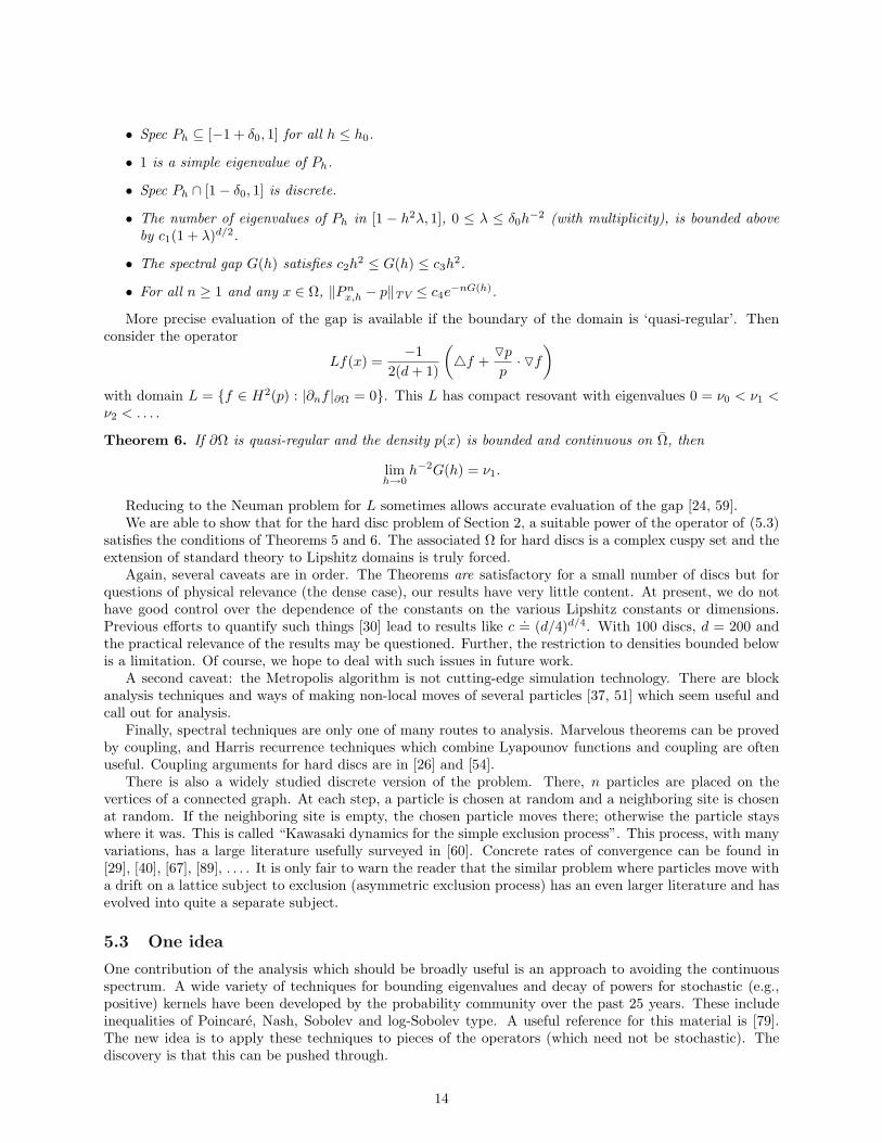
• Spec Ph ⊆ [−1 + δ0, 1] for all h ≤ h0.

• 1 is a simple eigenvalue of Ph.

• Spec Ph ∩ [1− δ0, 1] is discrete.

• The number of eigenvalues of Ph in [1 − h2λ, 1], 0 ≤ λ ≤ δ0h−2 (with multiplicity), is bounded above

by c1(1 + λ)d/2.

• The spectral gap G(h) satisfies c2h2 ≤ G(h) ≤ c3h2.

• For all n ≥ 1 and any x ∈ Ω, ‖Pnx,h − p‖TV ≤ c4e−nG(h).

More precise evaluation of the gap is available if the boundary of the domain is ‘quasi-regular’. Thenconsider the operator

Lf(x) =−1

2(d+ 1)

(4f +

Opp· Of

)with domain L = f ∈ H2(p) : |∂nf |∂Ω = 0. This L has compact resovant with eigenvalues 0 = ν0 < ν1 <ν2 < . . . .

Theorem 6. If ∂Ω is quasi-regular and the density p(x) is bounded and continuous on Ω, then

limh→0

h−2G(h) = ν1.

Reducing to the Neuman problem for L sometimes allows accurate evaluation of the gap [24, 59].We are able to show that for the hard disc problem of Section 2, a suitable power of the operator of (5.3)

satisfies the conditions of Theorems 5 and 6. The associated Ω for hard discs is a complex cuspy set and theextension of standard theory to Lipshitz domains is truly forced.

Again, several caveats are in order. The Theorems are satisfactory for a small number of discs but forquestions of physical relevance (the dense case), our results have very little content. At present, we do nothave good control over the dependence of the constants on the various Lipshitz constants or dimensions.Previous efforts to quantify such things [30] lead to results like c .= (d/4)d/4. With 100 discs, d = 200 andthe practical relevance of the results may be questioned. Further, the restriction to densities bounded belowis a limitation. Of course, we hope to deal with such issues in future work.

A second caveat: the Metropolis algorithm is not cutting-edge simulation technology. There are blockanalysis techniques and ways of making non-local moves of several particles [37, 51] which seem useful andcall out for analysis.

Finally, spectral techniques are only one of many routes to analysis. Marvelous theorems can be provedby coupling, and Harris recurrence techniques which combine Lyapounov functions and coupling are oftenuseful. Coupling arguments for hard discs are in [26] and [54].

There is also a widely studied discrete version of the problem. There, n particles are placed on thevertices of a connected graph. At each step, a particle is chosen at random and a neighboring site is chosenat random. If the neighboring site is empty, the chosen particle moves there; otherwise the particle stayswhere it was. This is called “Kawasaki dynamics for the simple exclusion process”. This process, with manyvariations, has a large literature usefully surveyed in [60]. Concrete rates of convergence can be found in[29], [40], [67], [89], . . . . It is only fair to warn the reader that the similar problem where particles move witha drift on a lattice subject to exclusion (asymmetric exclusion process) has an even larger literature and hasevolved into quite a separate subject.

5.3 One idea

One contribution of the analysis which should be broadly useful is an approach to avoiding the continuousspectrum. A wide variety of techniques for bounding eigenvalues and decay of powers for stochastic (e.g.,positive) kernels have been developed by the probability community over the past 25 years. These includeinequalities of Poincare, Nash, Sobolev and log-Sobolev type. A useful reference for this material is [79].The new idea is to apply these techniques to pieces of the operators (which need not be stochastic). Thediscovery is that this can be pushed through.

14

In more detail, consider the kernel Ph of (5.1) operating on L2(p). Write

Ph = Π + P 1h + P 2

h + P 3h

with Π the orthogonal projection onto the constants

P 1h (x, y) =

∑βj close to 1

βj(h)fj,h(x)fj,h(y), P 2h (x, y) =

∑110<

1−βjh2 < 9

10

βj,hfj,h(x)fj,h(y),

andP 3h = Ph −Π− P 1

h − P 2h .

The pieces are orthogonal, so powers of Ph equal the sum of powers of the pieces. Now P 1h and P 2

h can beanalyzed as above. Of course, bounds on eigenvalues and eigenfunctions are still needed. The continuousspectrum is hidden in P 3

h and one easily gets the crude bounds ‖P 3h‖L∞→L∞ ≤ ch−3d/2, ‖P 3

h‖L2→L2 ≤ (1−δ0).These can be iterated to give ‖(P 3

h )n‖L∞→L∞ ≤ ce−µn for a universal µ > 0 and all n > 1/h. Thus P 3h is

negligable.The work is fairly technical but the big picture is fairly stable. It holds for natural walks on compact

Riemannian manifolds [59] and in the detailed analysis of the one-dimensional hard disc problem [24, 27].The main purpose of this section is to show how careful analysis of an applied algorithm can lead to

interesting mathematics. In the next section, several further applications of Markov chain Monte Carlo aresketched. None of these have been analyzed.

6 Going Further, Looking Back; Contacts With Math, ContactsOutside Math

This section covers four topics. How someone outside probability can learn more about the present subject;a literature review on rates of convergence; a list of examples showing how a wide spectrum of mathe-matical tools have been used in analyzing Markov chains; and pointers to applications in various scientificapplications.

6.1 Going further

Suppose you are a ‘grown up mathematician’ who wants to learn some probability. The problem is, proba-bility has its own language and images. It’s a little like learning quantum mechanics — the mathematicaltools are not a problem but the basic examples and images are foreign. There are two steps. The first iselementary probability — the language of random variables, expectation, independence, conditional proba-bility and the basic examples (binomial, Poisson, geometric, normal, gamma, beta) with their distributiontheory. The second is mathematical probability — σ-algebras, laws of large numbers, central limit theory,martingales and brownian motion. Not to mention Markov chains.

The best procedure is to first sit in on an elementary probability course and then sit in on a first-yeargraduate course. There are hundreds of books at all levels. Two good elementary books are [39] and [78].This last is a very readable classic (don’t miss Chapter 3!). I use Billingsley’s book [9] to teach graduateprobability.

To learn about Monte Carlo, the classic book [44] is short and contains most of the important ideas.The useful books [15] or [62] brings this up to date. Two very good accounts of applied probability whichdevelop Markov chain theory along present lines are [7] and [10]. The advanced theory of Markov chains iswell covered by [3] (analytic theory), [38] (semi group theory) and [42] (Dirichlet forms). Two very usefulsurvey articles on rigorous rates of convergence are [67] and [79]. The on-line treatise [1] has a wealth ofinformation about reversible Markov chains. All of the cited works contain pointers to a huge literature.

6.2 Looking back

In this article, I have focused on using spectral theory to give rates of convergence for Markov chains. Thereare several other tools and schools. Two important ones are coupling and Harris recurrence. Coupling

15

is a ‘pure probability’ approach in which two copies of a Markov chain are considered. One begins instationarity, the second at a fixed starting point. Each chain evolves marginally according to the giventransition operator. However, the chains are also set up to move towards each other. When they hit acommon point, they “couple” and then move on together. The chain started in stationarity is stationary atevery step, in particular at the coupling time T . Thus, at time T , the chain starting from a fixed point isstationary. This approach transforms the task of bounding rates of convergence to bounding the couplingtime T . This can sometimes be done by quite elementary arguments. Coupling is such a powerful andoriginal tool that it must have applications far from its origins. A recent example is Robert Neel’s proof [71]of Liouville theorems for minimal surfaces.

Book-length treatments of coupling are [61] and [86]. The very useful path coupling variant in [11]and [35] is developed into a marvelous theory of Ricci curvature for Markov chains by [73]. The connectionsbetween coupling and eigenvalues is discussed in [12]. The coupling from the past algorithm of Propp–Wilson[77] has made a real impact on simulation. It sometimes allows exact samples to be drawn from intractableprobability distributions. It works for the Ising model. I clearly remember my first look at David Wilson’ssample of a 2, 000× 2, 000 Ising model at the critical temperature. I felt like someone seeing Mars througha telescope for the first time.

Harris recurrence is a sophisticated variant of coupling which has a well-developed ‘user interface.’ Thisavoids the need for clever, ad hoc constructions. The two chains can be exactly coupled for general statespaces when they hit a ‘small set.’ They can be driven to the small set by a Lyapounov function. A splendidintroduction to Harris recurrence is in [53]. A book-length development is [68]. The topic is often developedunder the name of “geometric ergodicity.” This refers to bounds of the form ‖Kl

x − π‖TV ≤ A(x)γl forA(x) > 0 and 0 < γ < 1. Observe that usually, proofs of geometric ergodicity give no hold on A(x) oron γ. In this form, the results are practically useless, saying little more than ‘the chain converges for largel.’ Bounds with explicit A(x), γ are called “honest” in the literature [53]. The work of Jim Hobert and hiscollaborators is particularly rich in useful bounds for real examples. For further discussion and references,see [23] and [50].

In the presence of geometric ergodicity, a wealth of useful auxiliary results become available. Theseinclude central limit theorems and large deviations bounds for averages 1/N

∑f(Xi) [56]. the variance of

such averages can be usefully estimated [46]. One can even hope to do ‘perfect sampling’ from the exactstationary distribution [55]. There has been a spirited effort to understand what the set-up required forHarris recurrence says about the spectrum [5, 6]. (Note that coupling and Harris recurrence do not dependon reversibility.)

6.3 Contact with math

The quest for sharp analysis of Markov chains has led to the use and development of tools from various areasof mathematics. Here is a personal catalog.

Group representations

Natural mixing schemes can sometimes be represented as random walk on groups or homogeneous spaces.Then, representation theory allows a useful Fourier analysis. If the walks are invariant under conjugation,only the characters are needed. If the walks are bi-invariant under a subgroup giving a Gelfand pair,the spherical functions are needed. A book-length discussion of this approach is in [14]. Sometimes, theprobability theory calls for new group theory. An example is the random walk on the group of upper-triangular matrices with elements in a finite field: starting at the identity, pick a row at random and addit to the row above. The character theory of this group is wild. Carlos-Andre has created a cruder “super-character” theory which is sufficiently rich to handle random walk problems. The detailed use of this requirednew formula [4] and leads to an extension of the theory to algebra groups in joint work with Isaacs and Theme[22, 34]. This has blossomed into thesis projects [45, 84, 85]. This thread is a nice example of the way thatapplications and theory interact.

16

Algebraic geometry

The creation of Markov chains to efficiently perform a sampling task can lead to interesting mathematics. Asan example, consider the emerging field of “algebraic statistics.” I was faced with the problem of generating(uniformly) random arrays with given row and column sums. These arrays (called contingency tables instatistics) have non-negative integer entries. For two-dimensional arrays, a classical Markov chain MonteCarlo algorithm proceeds as follows. Pick a pair of rows and a pair of columns at random; this delineatesfour entries. Change these entries by adding and subtracting in one of the following patterns:(

+ −− +

)or

(− ++ −

).

This doesn’t change the row/column sums. If the resulting array still has non-negative entries, the chainmoves there. Otherwise, the chain stays at the original array.

I needed to extend this to higher-dimensional arrays and similar problems on the permutation group andother structures where linear statistics are to be preserved. The problem is, the analog of the

(+ −− +

)moves

that statisticians have thought of do not connect the space. Bernd Sturmfels recognized the original(

+ −− +

)moves as generators of a determinental ideal and suggested coding the problem up as finding generators ofa toric ideal. All of the problems fit into this scheme and the emerging fields of computational algebra andGrobner bases allow practical solutions. The story is too long to tell here in much detail. The original ideasare worked out in [33]. There have been many extensions, bolstered by more than a dozen Ph.D. theses.A flavor of this activity and references can be gathered from [49]. The suite of computational resources inthe computer package Latte also contains extensive documentation. The subject of algebraic statistics hasexpanded in many directions. See [74] for its projection into biology and [76] for its projection into design ofexperiments. As usual, the applications call for a sharpening of algebraic geometric tools and raise totallynew problems.

For completeness I must mention that despite much effort, the running time analysis of the originalMarkov chain on contingency tables has not been settled. There are many partial results suggesting that(diam)2 steps are necessary and sufficient, where diameter refers to the graph with an edge between twoarrays if they differ by a

(+ −− +

)move. There are also other ways of sampling that show great promise [16].

Carrying either the analysis or the alternative procedures to the other problems in [33] is a healthy researcharea.

PDE

The analysis of Markov chains has a very close connection with the study of long time behavior of thesolutions of differential equations. In the Markov chain context we are given a kernel K(x, dy) with re-versible stationary measure π(dx) on a space X . Then K operates as a self-adjoint contraction on L2(π) viaKf(x) =

∫f(y)K(x, dy). The associated quadratic form E(f |g) = 〈(I −K)f, g〉 is called the Dirichlet form

in probability. A Poincare inequality for K has the form

‖f‖22 ≤ AE(f |f) for all f ∈ L2(π) with∫fdπ = 0.

Using the minimax characterization, a Poincare inequality shows that there is no spectrum for the operatorin [1 − 1/A, 1) (Markov operators always have 1 as an eigenvalue). There is a parallel ‘parity form’ whichallows bounding negative spectrum. If the spectrum is supported on [−1 + 1/A, 1 − 1/A] and the Markovchain is started at a distribution σ with L2 density g, then

‖Klσ − π‖2TV ≤ ‖g − 1‖22

(1− 1

A

)2l

.

This is a useful, explicit bound but it is often “off”, giving the wrong rate of convergence by factors of n ormore in problems on the symmetric group Sn. A host of more complex techniques can give better results.For example, K satisfies a Nash inequality if for all suitable f ,

‖f‖2+1/D2 ≤ A

E(f |f) +

1N‖f‖22

‖f‖1/D1 ,

17

and a log-Sobolev inequality if

L(f) ≤ AE(f |f), L(f) =∫f2(x) log

f(x)2

‖f‖22π(dx).

Here A, N and D are constants which enter into any conclusions. These inequalities are harder to establishand have stronger conequences. Related inequalities of Cheeger and Sobolev are also in widespread use. Forsurveys of this technology, see [69] or [79]. The point here is that most of these techniques were developedto study PDE. Their adaptation to the analysis of Markov chains requires some new ideas. This interplaybetween the proof techniques of PDE and Markov chains has evolved into the small but healthy field offunctional inequalities [5, 6] which contributes to both subjects.

Modern PDE is an enormous subject with many more tools and ideas. Some of these, for example, thecalculus of pseudo-differential operators and micro-local techniques, are just starting to make in-roads intoMarkov chain convergence [24, 25, 59].

A major omission in the discussion above are the contributions of the theoretical computer sciencecommunity. In addition to a set of problems discussed in the final part of this section, a host of broadlyuseful technical developments have emerged. One way of saying things is this: How does one establish anyof the inequalities above (from Poincare through log-Sobolev) in an explicit problem? Mark Jerrum andAlistair Sinclair introduced the use of paths to prove Cheeger inequalities (called conductance in computerscience). Dyer, Frieze, Lovasz, Kannan and many students and coauthors have developed and applied theseideas to a host of problems, most notably the problems of approximating the permanent of a matrix andapproximating the volume of a convex set. Alas this work suffers from the “polynomial time bug.” Thedevelopers are often satisfied with results showing that n17 steps suffice (after all, it’s a polynomial). Thisleads to theory of little use in practical problems. I believe that the ideas can be pushed to give useful resultsbut at the present writing much remains to be done. A good survey of this set of ideas is in [69].

6.4 Contacts outside math

To someone working in my part of the world, asking about applications of Markov chain Monte Carlo is alittle like asking about applications of the quadratic formula. The results are really used in every aspect ofscientific inquiry. The following indications are wildly incomplete. I believe you can take any area of science,from hard to social, and find a burgeoning MCMC literature specifically tailored to that area. I note thatessentially none of these applications is accompanied by any kind of practically useful running time analysis.Thus the following is really a list of open research problems.

Chemistry and physics

From the original application to hard discs through lattice gauge theory [66], MCMC calculations are amainstay of chemistry and physics. I will content myself by mentioning four very readable books, particularlygood at describing the applications to an outsider; I have found them useful ways to learn the science. Forphysics, [57] and [72]. For chemistry, [41] and [58]. A good feeling for the ubiquity of MCMC can be gleanedfrom the following quote from the introductory text of the chemist Ben Widom [88, p. 101]:

“Now, a generation later, the situation has been wholly transformed, and we are able to calculatethe properties of ordinary liquids with nearly as much assurance as we do those of dilute gasesand harmonic solids . . . . What is new is our ability to realize van der Waal’s vision through theintervention of high speeed digital computing.”

Biology

One way to access applications of MCMC in various areas of biology is to look at the work of the statisticalleaders of groups driving this research: Jun Liu (Harvard), Michael Newton (Wisconsin), Mike West (Duke)and Wing Wong (Stanford). The home pages of each of these authors contain dozens of papers, essentiallyall driven by MCMC. Many of these contain innovative, new algorithms (waiting to be studied). In addition,I mention the on-line resources “Mr. Bayes” and “Bugs.” These give hundreds of tailored programs forMCMC biological applications.

18

Statistics

Statisticians work with scientists, engineers and businesses in a huge swathe of applications. Perhaps 10 −−15% of this is driven by MCMC. An overview of applications may be found in the books [43] or [62]. For thevery active area of particle filters and their many engineering applications (tracking, filtering), see [36]. Forpolitical science-flavored applications, see [43]. Of course, statisticians have also contributed to the designand analysis of these algorithms. An important and readable source is [13].

Group theory

This is a much smaller application. It seems surprising, because group theory (the mathematics of symmetry)seems so far from probability. However, computational group theory, as coded up in the on-line libraries Gapand Magma, makes heavy use of randomized algorithms to do basic tasks such as deciding whether a group(usually given as the group generated by a few permutations or a few large matrices) is all of Sn(GLn). Is itsolvable, can we find its lower central series, normal closure, Sylow(p) subgroups, etc.? Splendid accounts ofthis subject are in [47] or [80]. Bounding the running time of widely-used algorithms such as the meat axeor the product replacement algorithm [75] are important open problems on the unlikely interface of grouptheory and probability.

Computer science (theory)

The analysis of algorithms and complexity theory is an important part of computer science. One centraltheme is the polynomial/non-polynomial dichotomy. A large class of problems such as computing the per-manent of a matrix or the volume of a convex polyhedron have been proved to be # p-complete. Theorists(Broder, Jerrum, Vazarani) have shown that while it may take exponential time to get an exact answer tothese problems, one can find provably accurate approximations in a polynomial number of operations (inthe size of the input) provided one can find a rapidly mixing Markov chain to generate problem instancesat random. The above rough description is made precise in the readable book [81]. This program calls formethods of bounding the running time of Markov chains. Many clever analyses have been carried out intough problems without helpful symmetries. It would take us too far afield to develop this further. Threeof my favorite papers (which will lead the reader into the heart of this rich literature) are the [63] analysisof the hit-and-run algorithm, the [52] analysis of the problem of approximating permanents and the [70]analysis of knapsack problems. All of these contain deep, original mathematical ideas which seem broadlyuseful. As a caveat, recent results of Widgerson suggest a dichotomy: either randomness can be eliminatedfrom these algorithms or P = NP . Since nobody believes P = NP , there is true excitement in the air.

To close this section, I reiterate that almost none of these applications comes with a useful running timeestimate (and almost never with careful error estimates). Also, for computer science, the applications are tocomputer science theory. Here the challenge is to see if practically-useful algorithms can be made from theelegant mathematics.

Acknowledgments

This paper leans on 30 years of joint work with students and coauthors. It was presented at the 25thanniversary of the amazing, wonderful MSRI. I particularly thank Marc Coram, Susan Holmes, KshitijKhare, Werner Krauth, Gilles Lebeau, Laurent Michel, John Neuberger, Charles Radin and Laurent Saloff-Coste for their help with this paper. A helpful referee and the patience of editor Susan Friedlander aregratefully acknowledged.

References

[1] Aldous, D. and Fill, J. (2002). Reversible Markov chains and random walks on graphs. Monograph.

[2] Allen, M. P. and Tildesely, D. J. (1987). Computer simulation of liquids. Oxford University Press,Oxford.

19

[3] Anderson, W. J. (1991). Continuous-time Markov chains. Springer Series in Statistics: Probability andits Applications. Springer-Verlag, New York. An applications-oriented approach.

[4] Arias-Castro, E., Diaconis, P., and Stanley, R. (2004). A super-class walk on upper-triangular matrices.J. Algebra, 278(2):739–765.

[5] Bakry, D., Cattiaux, P., and Guillin, A. (2008). Rate of convergence for ergodic continuous Markovprocesses: Lyapunov versus Poincare. J. Funct. Anal., 254(3):727–759.

[6] Barthe, F., Bakry, P., Cattiaux, P., and Guillin, A. (2008). Poincare inequalities for logconcave probabilitymeasures: a Lyapounov function approach. Elec. Comm. Probab., to appear.

[7] Bhattacharya, R. N. and Waymire, E. C. (1990). Stochastic processes with applications. Wiley Seriesin Probability and Mathematical Statistics: Applied Probability and Statistics. John Wiley & Sons Inc.,New York. A Wiley-Interscience Publication.

[8] Billera, L. J. and Diaconis, P. (2001). A geometric interpretation of the Metropolis-Hastings algorithm.Statist. Sci., 16(4):335–339.

[9] Billingsley, P. (1995). Probability and measure. Wiley Series in Probability and Mathematical Statistics.John Wiley & Sons Inc., New York, third edition. A Wiley-Interscience Publication.

[10] Bremaud, P. (1999). Markov chains, volume 31 of Texts in Applied Mathematics. Springer-Verlag, NewYork. Gibbs fields, Monte Carlo simulation, and queues.

[11] Bubley, B. and Dyer, M. (1997). Path coupling: a technique for proving rapid mixing in Markov chains.FOCS, pages 223–231.

[12] Burdzy, K. and Kendall, W. S. (2000). Efficient Markovian couplings: examples and counterexamples.Ann. Appl. Probab., 10(2):362–409.

[13] Cappe, O., Moulines, E., and Ryden, T. (2005). Inference in hidden Markov models. Springer Series inStatistics. Springer, New York. With Randal Douc’s contributions to Chapter 9 and Christian P. Robert’sto Chapters 6, 7 and 13, With Chapter 14 by Gersende Fort, Philippe Soulier and Moulines, and Chapter15 by Stephane Boucheron and Elisabeth Gassiat.

[14] Ceccherini-Silberstein, T., Scarabotti, F., and Tolli, F. (2008). Harmonic analysis on finite groups,volume 108 of Cambridge Studies in Advanced Mathematics. Cambridge University Press, Cambridge.Representation theory, Gelfand pairs and Markov chains.

[15] Chen, M.-H., Shao, Q.-M., and Ibrahim, J. G. (2000). Monte Carlo methods in Bayesian computation.Springer Series in Statistics. Springer-Verlag, New York.

[16] Chen, Y., Diaconis, P., Holmes, S. P., and Liu, J. S. (2005). Sequential Monte Carlo methods forstatistical analysis of tables. J. Amer. Statist. Assoc., 100(469):109–120.

[17] Conner, S. (2003). Simulation and solving substitution codes. Master’s thesis, Department of Statistics,University of Warwick.

[18] Critchlow, D. E. (1985). Metric methods for analyzing partially ranked data, volume 34 of Lecture Notesin Statistics. Springer-Verlag, Berlin.

[19] Diaconis, P. (1988). Group representations in probability and statistics. Institute of MathematicalStatistics Lecture Notes—Monograph Series, 11. Institute of Mathematical Statistics, Hayward, CA.

[20] Diaconis, P. and Graham, R. L. (1977). Spearman’s footrule as a measure of disarray. J. Roy. Statist.Soc. Ser. B, 39(2):262–268.

[21] Diaconis, P. and Hanlon, P. (1992). Eigen-analysis for some examples of the Metropolis algorithm.In Hypergeometric functions on domains of positivity, Jack polynomials, and applications (Tampa, FL,1991), volume 138 of Contemp. Math., pages 99–117. Amer. Math. Soc., Providence, RI.

20

[22] Diaconis, P. and Isaacs, I. M. (2008). Supercharacters and superclasses for algebra groups. Trans. Amer.Math. Soc., 360(5):2359–2392.

[23] Diaconis, P., Khare, K., and Saloff-Coste, L. (2008a). Gibbs sampling, exponential families and orthog-onal polynomials, with discussion. Statist. Sci., to appear.

[24] Diaconis, P. and Lebeau, G. (2008). Micro-local analysis for the Metropolis algorithm. Math. Z., toappear.

[25] Diaconis, P., Lebeau, G., and Michel, L. (2008b). Geometric analysis for the Metropolis algorithm onLipshitz domains. Technical report, Department of Statistics, Stanford University, preprint.

[26] Diaconis, P. and Limic, V. (2008). Spectral gap of the hard-core model on the unit interval. Technicalreport, Department of Statistics, Stanford University, preprint.

[27] Diaconis, P. and Neuberger, J. W. (2004). Numerical results for the Metropolis algorithm. Experiment.Math., 13(2):207–213.

[28] Diaconis, P. and Ram, A. (2000). Analysis of systematic scan Metropolis algorithms using Iwahori-Hecke algebra techniques. Michigan Math. J., 48:157–190. Dedicated to William Fulton on the occasionof his 60th birthday.

[29] Diaconis, P. and Saloff-Coste, L. (1993). Comparison theorems for reversible Markov chains. Ann. Appl.Probab., 3(3):696–730.

[30] Diaconis, P. and Saloff-Coste, L. (1996). Nash inequalities for finite Markov chains. J. Theoret. Probab.,9(2):459–510.

[31] Diaconis, P. and Saloff-Coste, L. (1998). What do we know about the Metropolis algorithm? J. Comput.System Sci., 57(1):20–36. 27th Annual ACM Symposium on the Theory of Computing (STOC’95) (LasVegas, NV).

[32] Diaconis, P. and Shahshahani, M. (1981). Generating a random permutation with random transposi-tions. Z. Wahrsch. Verw. Gebiete, 57(2):159–179.

[33] Diaconis, P. and Sturmfels, B. (1998). Algebraic algorithms for sampling from conditional distributions.Ann. Statist., 26(1):363–397.

[34] Diaconis, P. and Thiem, N. (2008). Supercharacter formulas for pattern groups. Trans. Amer. Math.Soc., to appear.

[35] Dobrushin, R. L. (1970). Prescribing a system of random variables by conditional distributions. Theor.Probab. Appl.– Engl. Tr., 15:453–486.

[36] Doucet, A., de Freitas, N., and Gordon, N. (2001). Sequential Monte Carlo in Practice. Springer-Verlag,New York.

[37] Dress, C. and Krauth, W. (1995). Cluster algorithm for hard spheres and related systems. J. Phys. A,28(23):L597–L601.

[38] Ethier, S. N. and Kurtz, T. G. (1986). Markov processes. Wiley Series in Probability and MathematicalStatistics: Probability and Mathematical Statistics. John Wiley & Sons Inc., New York. Characterizationand convergence.

[39] Feller, W. (1968). An introduction to probability theory and its applications. Vol. I. Third edition. JohnWiley & Sons Inc., New York.

[40] Fill, J. A. (1991). Eigenvalue bounds on convergence to stationarity for nonreversible Markov chains,with an application to the exclusion process. Ann. Appl. Probab., 1(1):62–87.

21

[41] Frenkel, D. and Smit, B. (2002). Understanding molecular simulation: From algorithms to applications,2nd edition. Computational Science Series, Vol 1. Academic Press, San Diego.

[42] Fukushima, M., Oshima, Y., and Takeda, M. (1994). Dirichlet forms and symmetric Markov processes,volume 19 of de Gruyter Studies in Mathematics. Walter de Gruyter & Co., Berlin.

[43] Gill, J. (2007). Bayesian methods: a social and behavioral sciences approach, 2nd ed. Statistics in theSocial and Behavioral Sciences. Chapman & Hall/CRC. Second edition.

[44] Hammersley, J. M. and Handscomb, D. C. (1965). Monte Carlo methods. Methuen & Co. Ltd., London.

[45] Hendrickson, A. O. F. (2008). Supercharacter theories of finite simple groups. PhD thesis, Universityof Wisconsin.

[46] Hobert, J. P., Jones, G. L., Presnell, B., and Rosenthal, J. S. (2002). On the applicability of regenerativesimulation in Markov chain Monte Carlo. Biometrika, 89(4):731–743.

[47] Holt, D. F., Eick, B., and O’Brien, E. A. (2005). Handbook of computational group theory. DiscreteMathematics and its Applications (Boca Raton). Chapman & Hall/CRC, Boca Raton, FL.

[48] Hora, A. and Obata, N. (2007). Quantum probability and spectral analysis of graphs. Theoretical andMathematical Physics. Springer, Berlin. With a foreword by Luigi Accardi.

[49] Hosten, S. and Meek, C. (2006). Preface. J. Symb. Comput., 41(2):123–124.

[50] Jarner, S. F. and Hansen, E. (2000). Geometric ergodicity of Metropolis algorithms. Stochastic Process.Appl., 85(2):341–361.

[51] Jaster, A. (2004). The hexatic phase of the two-dimensional hard disks system. Phys. Lett. A, 330(cond-mat/0305239):120–125.

[52] Jerrum, M., Sinclair, A., and Vigoda, E. (2004). A polynomial-time approximation algorithm for thepermanent of a matrix with nonnegative entries. J. ACM, 51(4):671–697 (electronic).

[53] Jones, G. L. and Hobert, J. P. (2001). Honest exploration of intractable probability distributions viaMarkov chain Monte Carlo. Statist. Sci., 16(4):312–334.

[54] Kannan, R., Mahoney, M. W., and Montenegro, R. (2003). Rapid mixing of several Markov chains fora hard-core model. In Algorithms and computation, volume 2906 of Lecture Notes in Comput. Sci., pages663–675. Springer, Berlin.

[55] Kendall, W. S. (2004). Geometric ergodicity and perfect simulation. Electron. Comm. Probab., 9:140–151 (electronic).

[56] Kontoyiannis, I. and Meyn, S. P. (2003). Spectral theory and limit theorems for geometrically ergodicMarkov processes. Ann. Appl. Probab., 13(1):304–362.

[57] Krauth, W. (2006). Statistical mechanics. Oxford Master Series in Physics. Oxford University Press,Oxford. Algorithms and computations, Oxford Master Series in Statistical Computational, and TheoreticalPhysics.

[58] Landau, D. P. and Binder, K. (2005). A Guide to Monte Carlo Simulations in Statistical Physics.Cambridge University Press, Cambridge.

[59] Lebeau, G. and Michel, L. (2008). Semiclassical analysis of a random walk on a manifold. Ann. Probab.,to appear(arXiv:0802.0644).

[60] Liggett, T. M. (1985). Interacting particle systems, volume 276 of Grundlehren der MathematischenWissenschaften [Fundamental Principles of Mathematical Sciences]. Springer-Verlag, New York.

[61] Lindvall, T. (2002). Lectures on the coupling method. Dover Publications Inc., Mineola, NY. Correctedreprint of the 1992 original.

22

[62] Liu, J. S. (2001). Monte Carlo Strategies in Scientific Computing. Springer Series in Statistics. Springer-Verlag, New York.

[63] Lovasz, L. and Vempala, S. (2006). Hit-and-run from a corner. SIAM J. Comput., 35(4):985–1005(electronic).

[64] Lowen, H. (2000). Fun with hard spheres. In Statistical physics and spatial statistics (Wuppertal, 1999),volume 554 of Lecture Notes in Phys., pages 295–331. Springer, Berlin.

[65] Macdonald, I. G. (1995). Symmetric functions and Hall polynomials. Oxford Mathematical Monographs.The Clarendon Press Oxford University Press, New York, second edition. With contributions by A.Zelevinsky, Oxford Science Publications.

[66] Mackenzie, P. (2005). The fundamental constants of nature from lattice gauge theory simulations. J.Phys. Conf. Ser., 16(doi:10.1088/1742-6596/16/1/018):140–149.

[67] Martinelli, F. (2004). Relaxation times of Markov chains in statistical mechanics and combinatorialstructures. In Probability on discrete structures, volume 110 of Encyclopaedia Math. Sci., pages 175–262.Springer, Berlin.

[68] Meyn, S. P. and Tweedie, R. L. (1993). Markov chains and stochastic stability. Communications andControl Engineering Series. Springer-Verlag London Ltd., London.

[69] Montenegro, R. and Tetali, P. (2006). Mathematical aspects of mixing times in Markov chains. Found.Trends Theor. Comput. Sci., 1(3):x+121.

[70] Morris, B. and Sinclair, A. (2004). Random walks on truncated cubes and sampling 0 − 1 knapsacksolutions. SIAM J. Comput., 34(1):195–226 (electronic).

[71] Neel, R. W. (2008). A martingale approach to minimal surfaces. J. Funct. Anal.,(doi:10.1016/j.jfa.2008.06.033). arXiv:0805.0556v2 [math.DG] (in press).

[72] Newman, M. E. J. and Barkema, G. T. (1999). Monte Carlo methods in statistical physics. TheClarendon Press Oxford University Press, New York.

[73] Ollivier, Y. (2008). Ricci curvature of Markov chains on metric spaces. Preprint, submitted, 2008.

[74] Pachter, L. and Sturmfels, B., editors (2005). Algebraic statistics for computational biology. CambridgeUniversity Press, New York.

[75] Pak, I. (2001). What do we know about the product replacement algorithm? In Groups and computation,III (Columbus, OH, 1999), volume 8 of Ohio State Univ. Math. Res. Inst. Publ., pages 301–347. de Gruyter,Berlin.

[76] Pistone, G., Riccomagno, E., and Wynn, H. P. (2001). Algebraic statistics, volume 89 of Monographs onStatistics and Applied Probability. Chapman & Hall/CRC, Boca Raton, FL. Computational commutativealgebra in statistics.

[77] Propp, J. G. and Wilson, D. B. (1996). Exact sampling with coupled Markov chains and applicationsto statistical mechanics. In Proceedings of the Seventh International Conference on Random Structuresand Algorithms (Atlanta, GA, 1995), volume 9, pages 223–252.

[78] Ross, S. M. (2002). A First Course in Probability, 7th Edition. Cambridge University Press, Cambridge.

[79] Saloff-Coste, L. (1997). Lectures on finite Markov chains. In Lectures on probability theory and statistics(Saint-Flour, 1996), volume 1665 of Lecture Notes in Math., pages 301–413. Springer, Berlin.

[80] Seress, A. (2003). Permutation group algorithms, volume 152 of Cambridge Tracts in Mathematics.Cambridge University Press, Cambridge.

23

[81] Sinclair, A. (1993). Algorithms for random generation and counting. Progress in Theoretical ComputerScience. Birkhauser Boston Inc., Boston, MA. A Markov chain approach.

[82] Stanley, R. P. (1999). Enumerative combinatorics. Vol. 2, volume 62 of Cambridge Studies in AdvancedMathematics. Cambridge University Press, Cambridge. With a foreword by Gian-Carlo Rota and appendix1 by Sergey Fomin.

[83] Taylor, H. M. and Karlin, S. (1984). An introduction to stochastic modeling. Academic Press Inc.,Orlando, FL.

[84] Thiem, N. and Marberg, E. (2008). Superinduction for pattern groups. Technical report, Departmentof Mathematics, University of Colorado, Boulder.

[85] Thiem, N. and Venkateswaran, V. (2008). Restricting supercharacters of the finite group of unipotentuppertriangular matrices. Technical report, Department of Mathematics, University of Colorado, Boulder.

[86] Thorisson, H. (2000). Coupling, stationarity, and regeneration. Probability and its Applications (NewYork). Springer-Verlag, New York.

[87] Uhlenbeck, G. E. (1968). An outline of statistical mechanics. In Cohen, E. G. D., editor, FundamentalProblems in Statistical Mechanics, volume 2, pages 1–19. North-Holland Publishing Co., Amsterdam.

[88] Widom, B. (2002). Statistical Mechanics: A Concise Introduction for Chemists. Cambridge UniversityPress, Cambridge.

[89] Yau, H.-T. (1997). Logarithmic Sobolev inequality for generalized simple exclusion processes. Probab.Theory Related Fields, 109(4):507–538.

24