The Market Value of Knowledge Protection: Evidence from a ...

† Leeds School of Business, University of Colorado, UCB 419, Boulder, CO 80309; [email protected] †† MIT Sloan School of Management, 100 Main Street, E62-478, Cambridge, MA 02142; [email protected]

The Market Value of Knowledge Protection: Evidence from a Natural Experiment

Kenneth A. Younge † Matt Marx ††

January 10, 2012

Preliminary Working Paper

Abstract

For firms to invest in R&D, it is essential that they capture value from the knowledge that they create. Firms earn supranormal returns only to the extent that they can exclude other firms from obtaining and using their proprietary knowledge. Ironically, we have little quantitative evidence regarding how firms protect knowledge aside from the patent system. But much knowledge is tacit, residing primarily in the minds of workers and leading firms to use employee non-compete agreements to prevent their leakage via interorganizational mobility. In a sample of public firms reporting R&D, we estimate the firm-level returns to non-competes using an apparently-inadvertent policy reversal in Michigan during the 1980s. We find that enforceable non-compete agreements boosted Tobin’s q by 26-30% in the short run, a result that is robust to a number of alternative specifications and placebo tests. This advantage, however, appears to be fleeting, perhaps the result of a long-run decrease in human capital investment by employees and the unavailability of talent in the local labor market.

Keywords: Tobin’s q, knowledge protection, employee mobility, non-compete agreements

JEL Classification: D8, G14, J24, K31, L25, O43

2

1 Introduction For firms to invest in R&D, it is essential that they be able to capture value from the knowledge

that they create. Firms may attempt to commercialize discoveries by licensing them to industry

incumbents (Teece 1986), though the intangible, non-rivalrous nature of information complicates

the process of securing rents in the market (Arrow 1962; Romer 1990). Alternatively, firms may

seek to avoid the problems of disclosure and opportunism (Stigler 1961; Williamson 1979) by

exploiting knowledge internally, improving operational efficiency and creating differentiating

products and services to compete directly with incumbents (Gans et al. 2002). Using knowledge

within the firm does not fully guard against expropriation, however: products can be reverse

engineered; processes can be leaked; and key employees can be hired away, taking proprietary

information with them (Liebeskind 1996). Regardless of which commercialization path they

pursue, firms earn supranormal returns only to the extent that they can exclude other firms

from obtaining and using the knowledge that they generate.

Perhaps the most frequently studied measure for establishing appropriability over

knowledge is patenting. Since Griliches (1981), numerous scholars have established that patent

protection contributes to the market value of firms (Cockburn & Griliches 1988; Schankerman

1998; Harhoff et al. 1999; Hall 2000; Bessen 2008). But patenting is not without its drawbacks.

To obtain a patent, applicants must publicly disclose proprietary information in a patent

application in exchange for what is only a temporary monopoly over the invention. Competitors

can also work around patents by reverse engineering and patents may in fact afford competitors

3

a partial technological map.1 Patent litigation can be costly, especially for small firms with

limited resources to defend themselves (Lerner 1995). Further, non-codifiable knowledge does

not lend itself to patent protection; software patents, for example, have questionable value (Hall

& MacGarvie 2010) and may offer minimal protection in fast-moving industries where the rate

of technology evolution outstrips the speed of patent examination (Hall & Ziedonis 2001).

Given the limitations and costs of protecting knowledge via patenting, firms may seek to

guard inventions and other information, such as customer lists, strategic plans, and tacit

knowledge residing in the heads of employees, through other “counterdiffusion” measures. One

such measure is a non-disclosure agreement, in which employees covenant to keep secret any

proprietary knowledge they have obtained during their employment. While such contracts lay

claim to all information that an employee either generates or becomes aware of while working at

the firm and banning its disclosure at any time, whether while under the firm’s employ or

thereafter, they are difficult to enforce given the legal challenge of documenting disclosure.

Alternatively, a firm may attempt to limit the potential damage from unauthorized disclosure

by disaggregating tasks such that any one individual has only partial knowledge (Rajan &

Zingales 2001). Disaggregation, however, may compromise the operational efficiency of the firm

and moreover does not prevent employees from leaving the firm with the proprietary knowledge

to which they did have access. A more thorough counterdiffusion policy is to simply prevent ex-

employees from taking proprietary knowledge with them to subsequent jobs in firms where that

1 The value of reading granted patents by competitors may be diminished somewhat by the delay in processing applications, which can take years. Since 2001, however, the U.S. Patent and Trademark Office has enabled electronic download of patent applications beginning 18 months after their submission.

4

knowledge could prove particularly advantageous. Indeed, courts have ruled that an ex-employee

working for a competitor is at substantial risk of “inevitably disclosing” information from their

prior job, even if attempting to honor a non-disclosure agreement (Whaley 1998). Accordingly,

U.S. states have granted firms the right to restrict the post-employment opportunities of a

firm’s current workforce by means of employee non-compete agreements (hereafter, “non-

competes”).

Non-competes are (sections of) employment contracts that place restraints on the behavior

of workers for a set period of time after they leave the firm, usually 1-2 years. A non-compete

either lists specific firms at which the ex-employee may not work or describes an industry within

which the employee is not allowed to compete either by joining or starting another company. As

such, non-competes restrict ex-employees from leaving to join competitors (Fallick et al. 2006).2

Non-competes are generally easier to enforce than non-disclosure agreements because it is easier

to verify that an ex-employee is working for a competitor than to establish that said worker has

leaked proprietary information. Non-competes are widely used by firms in a variety of technical

industries (Marx 2011) and appear in nearly 90% of venture capital contracts (Kaplan &

Stromberg 2001).

In stark contrast to the extensive literature on the market value of patent protection, we

know very little regarding how counterdiffusion measures, including employee non-compete

agreements, impact firm-level outcomes. This gap is particularly puzzling given that multiple

2 Non-disclosure agreements typically allow an employee to list “prior inventions” which are excluded from the employer’s claim. In this way, employees are able to separate intellectual property that they created while not under the jurisdiction of the firm from that supported by the employer's R&D activities. By comparison, non-compete agreements typically do not allow the employee to identify skills or expertise they acquired previously as not being governed by the contract.

5

surveys of appropriability mechanisms suggest that the ability to keep proprietary information

private via secrecy is as important to R&D managers as patenting, if not more so (Levin et al.

1987; Cohen et al. 2000; Arundel 2001). In the only known study of non-competes and firm

value, Garmaise (2011) finds that increased non-compete enforcement drives down R&D

spending per capita but does not influence either return on equity or the market-to-book ratio.

The only tangible benefit to firms in Garmaise’s study is the ability to pay lower wages; if so,

then it seems puzzling that most states in the U.S. sanction the use of non-compete agreements

in light of the aforementioned costs to individuals as well as negative implications at the

regional level. 3

In this study, we address these questions by leveraging an apparently-unexpected reversal

of non-compete policy in Michigan during the 1980s. We find that Michigan firms reporting

R&D, which were able to use non-competes following the policy reversal, enjoyed a initial boost

in Tobin’s q relative to firms in other states. This initial boost is robust to a variety of

alternative specifications including changes in business-combination laws, and we fail to recreate

the effect in a series of placebo regressions. Moreover, this effect is increasing in R&D spending

but decreasing in the number of patents, suggesting that patenting and non-competes may act

as substitutes. This initial boost in q does however attenuate over time, suggesting that firms’

3 Stuart and Sorenson (2003) find that the spawning rate of new biotech firms following liquidity events was attenuated in states that more strictly enforce non-compete agreements. Further evidence for the deleterious effect of non-competes on the entrepreneurial environment was found by Samila and Sorenson (2010), who found that venture capital yielded fewer patents, jobs, and new establishments where non-competes were enforced. Beleznon and Schankerman (2011) show that non-competes act as a brake on the diffusion of university inventions. Marx, Singh, and Fleming (2011) provide evidence that non-compete enforcement leads to an exodus of skilled workers, who seek more favorable employment terms in regions that restrict the use of non-competes.

6

immediate actions to capitalize on the ability to more closely hold proprietary information may

eventually be offset by the actions of employees or actors in the external labor market.

2 Empirical Strategy Establishing the impact of non-competes on firm value is nontrivial for several reasons. First,

although considerable state-level variation exists, unobserved heterogeneity renders cross-

sectional estimates of dubious value. Second, while several states have made changes to their

non-compete enforcement statutes, many of these involve slight modifications that may not

substantially affect the behavior of either firms or their employees. For example, in 2008 Idaho

granted judges greater latitude in establishing whether an employer had a “legitimate business

interest” in enforcing the non-compete. While such a change in the law may affect the behavior

of judges, it is unclear to what extent its reverberations would be felt outside the courtroom. In

a field study of non-competes, Marx (2011) found that none of the ex-employees in his sample

who took “career detours” in order to avoid infringing upon the non-compete were actually taken

to court; rather, in believing that a non-compete was enforceable, they made worst-case

assumptions about how a potential lawsuit would play out. Accordingly, for purposes of our

identification strategy we want to make use of a policy change that involved not just a

procedural modification of the law but a substantial reversal. We believe that Michigan offers

such an opportunity.

Non-compete enforcement in Michigan had long been governed by Public Act No. 329 of

1905, Section 1: “All agreements and contracts by which any person, copartnership, or

corporation agrees not to engage in any avocation, employment, pursuit, trade, profession or

7

business, whether reasonable or unreasonable, partial or general, limited or unlimited, are

hereby declared to be against public policy and illegal and void.”4 This Act prohibited the use of

non-competes until 1985, when the Michigan Antitrust Reform Act (MARA) was passed. The

stated purpose of MARA was to centralize and standardize existing doctrine regarding antitrust

policy, including collusion and price-fixing (Bullard 1985). Doing so involved both introducing a

new body of law regarding antitrust (i.e., MARA itself) and repealing existing laws and acts

that touched upon such issues. Among the statutes repealed was Public Act No. 329, which

largely addressed antitrust issues including “maintain[ing] a monopoly of any trade” (Sections 2-

4) and “combinations in restraint of trade” (Sections 5 and 6).

The available evidence suggests that Public Act No. 329 was repealed as part of MARA

due to its antitrust implications, and not specifically because of a desire to change the law

regarding employee non-compete agreements. More than twenty pages of legislative analysis by

both House and Senate subcommittees in Michigan (Bullard 1985) discuss antitrust extensively

as the motivation behind MARA but fail to mention “non-competes”, “covenants not to compete”,

“restrictive covenants” in the deliberations leading up to the passage of the new statute—and the

accompanying repeal of obsolete statutes. Thus it appears that the legislature did not realized it

had repealed the ban on non-competes.

Further evidence for the inadvertent nature of Michigan’s non-compete reversal is found

during the period after MARA was enacted. Although we could not locate any discussion of

4 The language of the Act resembles that of California’s Business and Profession Code Section 16600: “Except as provided in this chapter, every contract by which anyone is restrained from engaging in a lawful profession, trade, or business of any kind is to that extent void.”

8

Michigan’s non-compete policy in law journals just prior to 1985, multiple articles appeared in

the months following the reversal (Alterman 1985; Levine 1985; Sikkel & Rabaut 1985),

apparently as a result of practicing lawyers having reviewed the repealed statutes. These articles

highlighted the new enforceability of non-competes in the state, news which may have spread

among law firms, which would have then informed their clients in hopes of generating

contractual or prosecutorial work (Bagley 2006). These developments suggest that the legal

community was not aware of the potential for the law to be reversed but learned of the change

quickly thereafter.

Moreover, less than two years after the passage of MARA, the Michigan legislature

amended MARA section 4(a), effective retroactively to the enactment of MARA. Importantly,

the reasonableness doctrine did not reinstate the pre-MARA ban on non-compete agreements

but merely provided some limitations regarding the scope and duration of non-competes, as is

common in most states that permit their enforcement. This post-hoc, retroactive amendment

suggests that the legislature later realized it had repealed the non-compete ban without fully

considering its implications. Indeed, both House and Senate legislative analyses of the section

4(a) amendment to MARA state that a key motivation for the amendment was “to fill the

statutory void” (Trim 1987).

Interviews with Michigan labor lawyers active at the time of MARA are supportive of an

interpretation of the repeal as inadvertent. Robert Sikkel (2006) reported, “There wasn’t an

effort to repeal [the ban on] non-competes. We backed our way into it. The original prohibition

was contained in an old statute that was revised for other issues. We were not even thinking

9

about non-compete language. All of a sudden the lawyers saw no proscription of non-competes.

We got active and the legislature had to go back and clarify the law.” His account was

independently corroborated in a separate interview with Louis Rabaut (2006): “There was no

buildup, discussion, or debate of which I was aware—it was really out of the blue. As I talked to

others, this appeared to be a rather uniform reaction. I have never been able to identify any

awareness—and I examined this at the time—that this was a conscious or intentional act. It was

part of the antitrust reform and it may have been overlooked. I am unaware of anyone that

lobbied for the change.”

Alternative Explanations

Taken together, these pieces of evidence suggest that the MARA policy reversal was an

unanticipated and exogenous event that provides the opportunity for a natural experiment as

far as the change in non-compete enforcement policy is concerned. Yet certain aspects of the

reform may suggest alternative explanations for the results we find. We note four principal

competing hypotheses here and address each with separate analyses in the robustness section.

Anti-trust Reforms. First, our identification strategy assumes that aspects of MARA

other than the reversal in the enforcement of non-compete agreements do not increase the

valuation of firms in Michigan. We also note that MARA, although it unintentionally repealed

the ban on non-competes, purposefully set in force antitrust reforms designed to reduce price-

fixing and collusion. Said antitrust reform might have favored small firms at the expense of

larger ones, but its overall effect on Tobin’s q is unclear. We therefore perform several placebo

10

analyses of anti-trust reforms in states other than Michigan that were similar to MARA and

that occurred around the same time as MARA.

Automotive Industry. Second, given the concentration of automobile production in

Michigan (see Singleton 1992 for an overview), one might wonder whether an effect in Michigan

is primarily representative of the automotive industry. While we include industry fixed effects in

our specification in order to estimate only within-industry variation, we also take the additional

step of performing several robustness tests and subsample analyses to rule out the possibility

that the effect is attributable solely to the automobile industry.

Midwest Effect. Third, we investigate whether the effect we identify in Michigan

represents a larger “Midwest effect” that spuriously relates to MARA. To rule out this possibility,

we perform several placebo analyses of other Midwest states by inserting firms from those other

states into the analysis in place of Michigan firms.

Business Combination Laws. Fourth, prior research highlights that many states

passed business combination (BC) laws in the late 1980s (Bertrand & Mullainathan 2003), not

long after MARA. By reducing the threat of hostile takeover, BC laws may weaken corporate

governance and increase the opportunity for managerial slack, leading to a decrease in firm

valuation (Giroud & Mueller 2010). To the extent that BC laws might depress the market

valuations of firms in comparison states during the post-MARA period, a difference-in-

differences analysis would over-estimate the effect of MARA in Michigan. To control for this

possibility, we include an indicator variable for the passage of a business combination law in

each firm’s state of incorporation.

11

3 Data and Methods The sample includes firm-level data from Compustat for 1977 through 1996, the 10 year window

before and 10 year window after MARA. We selected all publically listed firms in Michigan and

a set of control states, including Alaska, California, Connecticut, Minnesota, Montana, North

Dakota, Nevada, Oklahoma, Washington, and West Virginia, which did not enforce non-

competes before or after MARA (Stuart & Sorenson 2003). We limited the sample to firms that

reported R&D expenses, were headquartered in either Michigan or a control state, were

publically listed prior to MARA, and were not in the agriculture, forestry, fishing, or financial

industries, resulting in a preliminary sample of 6,164 records. State affiliation was based on the

location of corporate headquarters (not the state of incorporation) and historical moves between

states were corrected based on the “comphist” table of corporate moves in Compustat. Given

that ratios take on extreme values when the scaling variable becomes too small or too large, we

dropped the top and bottom 0.1% of observations for Tobin’s q and the top 1.0% of

observations for R&D Intensity, dropping 94 observations.

Next, we stratified and matched the sample through Coarsened Exact (CEM) (Iacus et al.

2011). Coarsened Exact Matching is a non-parametric algorithm used to improve the common

support between treated and control observations and to reduce model dependence (see Azoulay

et al. 2010 for a recent application). Coarsened Exact Matching segments the joint distribution

of covariates into a limited number of strata, and then weights observations from each strata to

match observations between the treatment and control groups. We matched on the basis of

Assets, Beta, and Debt-to-Equity, measured on a pre-MARA basis in order to ensure that the

12

matching criteria were not influenced by the policy reversal. Rather than assign arbitrary cut-

points, we relied on the automatic CEM implementation in Stata to determine the number and

boundaries of each strata based on an objective function and Sturge’s rule (Iacus et al. 2011).

The matched (but original and unchanged) observations were then retained and analyzed in the

analysis described below. Our implementation of CEM dropped 2,613 observations from the

sample, producing a sample size of 3,457 observations for the basic analysis.5

Because CEM matches most observations in Michigan and only matches similar

observations in comparison states, CEM can produce a sample that is more representative of the

types of firms in the treated state (Michigan). It is possible, therefore, for CEM to limit the

generalizability of estimates made from this sample, although the matching procedure itself

should increase the internal validity and causal interpretation of the estimates. To assess the

generalizability of our sample, we calculated the relative distribution of public firms across SIC2

industry groupings and identified industries with a disproportionate representation in Michigan.

As might be expected, the automobile and transportation equipment industries stand out in the

Michigan economy, although this is also true, to a lesser extent, for industries associated with

the production of metal products, steel, glass, cement, rubber, plastics, wood and furniture. We

undertook additional robustness checks (reported below) to ensure that our results are not

disproportionately related to those industries.

5 While matching methods can improve common support and causal inference, our use of CEM also dropped 43% of the sample. Reductions of this magnitude can weight results toward the type of firms observed in the treated group (i.e., firms of a similar size, risk and capital structure as firms in Michigan). We therefore conducted sensitivity checks using less stringent matching; when we manually stratified observations into only 5 bins per matched variable, we dropped 10% of the sample and obtained results that were qualitatively similar to our key findings.

13

Next, we merged firm-level observations for Patents (and patent citations) into the

existing sample based on data from the NBER Patent Citations Data File (Hall et al. 2001; Hall

et al. 2005). Patents was assumed to be zero when a firm did not have a patenting record, and a

dummy variable (Patenting Indicator) was created to control for firms with missing patent

records. In models with covariate controls, an additional 429 observations were dropped due to

missing data, producing a final sample size of 3,028 observations.

Dependent Variable

Consistent with prior research on the valuation of intangible assets (e.g., Hirschey 1982;

Villalonga 2004; Hall et al. 2005), the dependent variable in all of our models is Tobin’s q.

Recent research suggests that computationally costly approaches to the calculation of Tobin’s q

(e.g., Lindenberg & Ross 1981; Lewellen & Badrinath 1997) may induce sample-selection bias

due to data unavailability (DaDalt et al. 2003). We therefore used a simple approximation of

Tobin’s q, defined as the market value of common stock + book value of total assets – book

value of common equity, all divided by the book value total assets.6 As an unreported

robustness check, we also tested the Chung & Pruitt (1994) approximation of Tobin’s q and

found similar results. Prior research also suggests that intangible assets may have a

multiplicative rather than additive effect on value due to fixed costs in developing intangible

assets, and that therefore a semi-log functional form is strongly preferred over a linear functional

6 This calculation for Tobin’s q in terms of fields from COMPUSTAT = ((PRCC_F * CSHO) + AT – CEQ ) / AT.

14

form for our regression equation. We therefore take the natural logarithm of Tobin’s q as our

dependent variable.7

Explanatory Variables

The DD treatment group variable, Michigan, is an indicator for firms located in Michigan based

on the historical location of the firm’s corporate headquarters. Compustat’s historical files

provide information on firms’ historical locations required for this variable. The DD ‘after’

variable, After, is an indicator that equals one for all years following 1986, and zero otherwise.

Following prior DD research, we then created an interaction variable Michigan * After and used

this variable to identify the treatment effect of MARA.

Although MARA was enacted in 1985, which could suggest 1986 and later as the “treated”

period for our analysis; we instead used 1987 and later as the treatment period. It was not until

late 1985 that legal scholars first recognized the change in the enforcement of non-competes (as

opposed to the general anti-trust provisions) in the legislation and published their findings in

the Michigan Bar Journal (Levine 1985; Sikkel & Rabaut 1985). We assume that it would have

taken some time, perhaps several months, for information about the policy change to diffuse

from the legal community to firms and R&D managers in particular. Moreover, unlike individual

mobility decisions, which can be acted upon quickly by workers, organizational changes to take

advantage of the newfound ability to protect trade secrets may have taken additional time to

implement. For these reasons, we believe that 1987 is the first year in which changes made by

7 Logging the dependent variable also helps to control for heteroskedasticity in the residuals.

15

firms in response to MARA would be fully reflected in Tobin’s q and thus use it and later as the

treatment period for the analysis.8

In addition to the main effect of MARA on Tobin’s q, we explore two moderating factors:

R&D Intensity and Patents. To address concerns of endogeneity , we use the pre-MARA value

for each moderator and hold it constant throughout the post-MARA period.9 First, given that

non-competes in theory serve to block the diffusion of trade secrets, we anticipate that the

impact of enforceable non-competes on q should be increasing in the level of R&D. We measured

R&D Intensity as the level of R&D expense divided by total sales (e.g., Cohen et al. 1987;

Cohen & Levinthal 1989), interacting it with the Michigan * After interaction and mean-

centering it at zero to simplify interpretation of the interaction effects. Second, we examined the

extent to which the effectiveness of non-competes is moderated by other means of protecting

intellectual property. Our variable here is the number of eventually-granted patent applications

for a given year, though we have weaker priors as to the effect of the variable. On the one hand,

one might theoretically expect non-compete agreements to most benefit firms that have not

taken other steps to protect their intellectual property by patenting (as suggested by Samila &

Sorenson 2011). Moreover, the act of codifying knowledge in a patent may help to reduce the

firm’s dependency on a particular employee; firms that do not – or cannot, due to the tacit

nature of that firm’s knowledge – undertake codification may be at greater risk of harm if an

8 We also note that these complications in determining a sharp break-point in the diffusion of understanding about the policy change prevent us from undertaking other methods of analysis, such as calculating a cumulative abnormal return around the time of the policy change. Instead, we perform a pre-to-post analysis of the average effect of MARA (in a difference-in-differences specification) covering the 10 years before and after MARA, and then examine the year-by-year effects of MARA in each year over the time period. 9 We checked the sensitivity of that approach by also testing the 5 year pre-MARA average of each moderator and found similar results. Results are available from the authors.

16

employee departs and thus benefit more from non-competes. A strong substitution effect

between non-compete and patent protection is yet to be established, however,10 so the extent to

which patenting moderates the effect of enforceable non-competes on firm value may not be

large.

Control Variables

Finally, we added covariate controls into most of our models to adjust for potential differences

in trends between the treated state (Michigan) and the group of comparison states. While trends

over time in the group of comparison states serve as the basic control in a differences-in-

differences specification, additional covariates help to control for specific regional differences. At

the state level, we control for personal income and the change in state employment. At the firm

level, we controlled for each firm’s financial condition and other characteristics that might affect

a firm’s market valuation. We also added Business Combination Law as an indicator variable to

control for the passage of a business combination law in each firm’s state of incorporation. Table

1 presents summary statistics for the mean, standard deviation, and range of all variables for

the final matched sample (n=3,028). All of the control variables are also summarized in Table 1.

----- Insert Table 1 about here -----

Model Specification

The Michigan natural experiment lends itself to a difference-in-differences (DD) model

specification. In our analysis, we assigned firms in Michigan to the treatment group in that firms

in Michigan experienced the MARA policy change. The control group is composed of firms in 10 Marx et al. (2009) found that patenting rates in Michigan were largely unchanged after the MARA policy reversal.

17

Alaska, California, Connecticut, Minnesota, Montana, North Dakota, Nevada, Oklahoma,

Washington, and West Virginia — states that placed substantial restrictions on the enforcement

of non-competes both before and after MARA (Malsberger et al. 2002; Stuart & Sorenson 2003).

Pre-Post Analysis. For our basic DD analysis (Tables 3 and 4), we used ordinary least

squares (OLS) and robust standard errors clustered by firm to estimate the following regression

equation without covariate controls:

ln(qi) = β0 + β1Michigani + β2Afteri + β3(Michigani*Afteri) + Tt + Ij + εi (1)

Ln(qi) is the natural logarithm of Tobin’s q for each i firm-year observation, Ij is a vector of

industry dummy variables at the SIC-4 level, Tt is a vector of year dummy variables, and εi is

the error term. We included as series of annual indicators to control for aggregate changes in

Tobin’s q over time due to business cycles, market swings, and so forth; we included industry

indicators to control for between-industry differences.

For the moderated DD analyses (Tables 5 – 9), we added interactions for R&D Intensity

(RDI) and Patents, as well as a set of covariate control variables (Xi), and estimated the

following regression equation:

ln(qi) = β0 + β1Michigani + β2Afteri + β3(Michigani*Afteri) + β4RDIi + β5(Michigani*RDIi) + β6(Afteri*RDIi) + β7(Michigani*Afteri*RDIi) + β8Patentsi + β9(Michigani*Patentsi) + β10(Afteri*Patentsi) + β11(Michigani*Afteri*Patentsi) + δXi + Tt + Ij + εi (2)

Year-by-Year Analysis. The standard DD specifications above estimate the average

pre-post effect of MARA. To test the dynamic effect of MARA over time, we regressed a ‘year-

by-year’ (YBY) difference-in-differences model covering the 10 years before and 10 years after

18

MARA (for recent examples of this method, see Kerr & Nanda 2009; Beck et al. 2010). The

year-by-year model removes the After variable and the Michigan*After interaction, and replaces

those variables with a series of Michigan*Year interactions, omitting 1986 as the MARA

reference year. In this manner, the YBY model estimates (in one model) the main effect of

MARA in each of the 20 years from 1976 through 1996, relative to the omitted year of 1986. As

indicated earlier, we believe that the managerial community first became aware of MARA

during 1986, making it the suitable reference year against which to compare results for years

from both before and after the policy change. The year-by-year model is used as the basis for

Figure 3, and is estimated from the following equation:

ln(qi) = β0 + β1Michigani + + Ij + Tt + εi (3)

Michigani*Yeart+q is a series of 20 separate indicator variables modeling the passage of time in

the difference-in-differences effect of MARA omitting the reference year of 1986 where q=0; Tt is

a vector of Yeari dummy variables (as specified before); all other variables are the same as

specified earlier.

Finally, we used a statistical simulation technique to test whether the effect of MARA

attenuated over time after MARA. From the YBY model we took the vector of coefficient

estimates for the effect of Michigani*Yeart+q and the variance-covariance matrix (both estimated

from equation 3), and simulated 1,000 effect sizes for each year of the post-MARA period. Given

the 10 years of the post-MARA period, this simulation approach allowed us to generate a new

dataset of 10,000 observations with which to test the trajectory of the effect size of MARA in

the post-MARA period. This simulation techniques allows us to take into account uncertainty as

!(Michigani *Yeart+qq=!10

10

" )

19

to the precision of the coefficient estimates for the main effect of MARA in the post-MARA

period obtained from estimating equation 3. We then used OLS, with robust standard errors

clustered by year, to estimate the following equation:

EffectSizejt= α0 + α1Yearjt + εjt (4)

The new variable Year varies from 1987 through 1996 and reflects the linear trend in the effect

size of MARA in the post-MARA years; j indexes each of the (1,…, 1000) simulations; t indexes

each of the 10 post-MARA years.

4 Results We begin with a simple visualization of the temporal trend in Tobin’s q from 1977 through

1996. We select a window of 10 years about MARA in that it represents an even, round number

not subject to analyst selection, ending before the start of the Internet bubble in the late 1990s

(Moeller et al. 2004). Figure 1 plots the yearly average of Tobin’s q for firms in Michigan and

for firms in comparison states. We calculate the within-industry average of Tobin’s q (weighting

within-industry averages by firm asset size) and then averaged results across industries, plotting

the final result by year and by group (Michigan or comparison states). Figure 1 suggests that

average within-industry trends in Tobin’s q were roughly similar between Michigan and

comparison states before MARA, but then diverged significantly after MARA. We also observe

that much of the difference-in-differences effect appears to derive from an increase in Tobin’s q

in Michigan after MARA.11

11 While our empirical strategy does not require an increase in Tobin’s q in Michigan after MARA (as opposed to a decrease in comparison states), for it is possible for a treatment effect to work against an otherwise counterfactual downward trend in the

20

----- Insert Figure 1 about here -----

Table 2 compares the before-to-after average difference in Tobin’s q for firms in Michigan

to matched firms in comparison states over the same time period. Table 2 indicates that Tobin’s

q rose by 0.55 points in Michigan, from a value of 1.25 before MARA 1.80 in after MARA while

the trend in the control states was more modest, growing only from 1.61 to 1.66. We report a

DD statistic of 0.50, representing an 40.0% increase in Tobin’s q over the pre-MARA Michigan

average.


Moving to a regression framework, we first reconcile the univariate difference-in-differences

results reported in Table 2 to a series of simple models that exclude any possibly endogenous

factors. Limited to indicators for Michigan, the post-MARA period, and their interaction, these

models are reported in Table 3. The DD effect of 0.50 in Panel B - Table 2 is equivalent to the

coefficient estimate of 0.4979 reported in Column 1 of Table 3, the basic model with no year

fixed effects, no industry fixed effects, no matching, and an un-logged value of Tobin’s q as the

dependent variable. Having thus reconciled the start of the regression analysis, we then switch

to the natural logarithm of Tobin’s q in Column 2 and thereafter to better control for the non-

linearity of intangible assets (Hirsch & Seaks 1993) and heteroskedasticity. Given a semi-log

specification, we can now interpret coefficients in Column 2 (and subsequent models) as a

percentage change in Tobin’s q. In Column 3 we add industry fixed effects at the SIC-4 level; in

Column 4 we add year indicators; and finally in Column 5 we restrict the sample to those

comparison group, it is nevertheless reassuring to observe that the onset of MARA coincides with a general increase in the trend in Tobin’s q in Michigan, a finding that is consistent with a less complicated understanding of the effect of MARA.

21

observations matched by CEM. Column 5 suggests that enforceable non-competes increased the

market value of firms in Michigan after MARA by 16.53%, with statistical significance at the

1% level.


Before proceeding to analysis with the full set of covariates, we wish to address a key

concern with our methodology: that the anti-trust nature of the MARA reform may have

conflated with the imposition of enforceable non-competes in producing the estimates. As noted

earlier, MARA intentionally set in force antitrust reforms designed to reduce price-fixing and

collusion in addition to unintentionally repealing the ban on non-competes. While it would seem

unlikely that tougher antitrust enforcement could raise the value of the large, publicly-traded

firms that are the subject of this study, direct confirmation of this assumption is not possible

using the Michigan experiment given the simultaneous introduction of enforceable non-compete

agreements. We therefore perform two placebo tests of anti-trust reforms in states other than

Michigan, that were similar to MARA and that occurred around the same time as MARA, to

provide evidence for the assumption.

Folsom reports (1991: page 955, footnote 54) that Texas and Delaware also enacted major

new antitrust legislation of a similar nature around the same time as MARA. Because these

other reforms did not repeal the ban on non-competes or change non-compete enforcement,

these are attractive candidates for independently assessing the effect of a very similar antitrust

reform on Tobin’s q. In Column 1 of Table 4 we test the Texas Free Enterprise and Antitrust

Act of 1983 by substituting Texas for Michigan in the analysis and changing the After variable

22

to 1985. We find an insignificant coefficient on the Texas * After variable in this model,

consistent with our expectations. In Column 2 of Table 4 we tested the Delaware Antitrust Act

of 1980 by substituting Delaware for Michigan in the analysis and changing the After variable to

1982.12 We again found an insignificant coefficient on Delaware * After, providing additional

evidence that antitrust reforms in themselves should not have raised levels of Tobin’s q during

this period.


We now move, in Table 5, to an analysis using the full set of covariates described above in

Table 1. While the comparison group serves as the basic control mechanism for any number of

unspecified covariates in a diff-in-diff specification, the inclusion of specific covariates may help

to control for a departure from the equal trends assumption (Blundell & Costa-Dias 2000).

Across Table 5, we find that Age and Dividend Policy payouts have a negative and significant

association with Tobin’s q, while Revenue Growth, Net Income, and Return on Assets all have a

positive and significant association with Tobin’s q. These findings are generally consistent with

the view that growth firms are younger (Cooley & Quadrini 2001), pay lower dividend yields

(Gaver & Gaver 1993), and have higher market valuations (Smith & Watts 1992); it is also

straightforward that better performing firms have higher market valuations. All other control

variables are insignificant.13 After adding covariate controls, we find that the basic Michigan *

12 We assign firms to states based on their location of corporate headquarters, and not their state of incorporation. While more than 50% of all public firms incorporate in the state of Delaware (Daines 2001), only 0.23% of firms in our sample are actually headquartered in Delaware. The lack of Delaware firms prevented us from matching observations in the analysis tested in Column 2 of Table 4, and so this model does not use CEM. 13 Ex ante, we included a broad range of covariates to control for potential differences in trends between Michigan and the comparison states that could also affect Tobin’s q. Given that many of the control variables turned out to be insignificant, we

23

After effect of MARA increased the market value of firms in Michigan by 11.76%, with

statistical significance at a 7% level.


Next, we test the moderating effect of R&D Intensity and Patents by adding three-way

interactions for Michigan * After * R&D Intensity (Column 2) and Michigan * After * Patents

(Column 3). We predicted earlier that the effect of MARA on Tobin’s q should be increasing in

R&D spending which is confirmed in Column 2. Regarding patenting, while we find statistically

significant evidence in Column 3 that the impact of non-competes is decreasing in patenting, the

economic significance appears quite small. In Column 4, we include all variables and interactions

together and prefer this as our “Final Specification.” In this model we find that the basic

Michigan * After effect of MARA is significant at the 5% level and roughly equivalent to a

25.88% increase in Tobin’s q (although we adjust that estimate slightly to 30.00% when

predicting outcomes below). We interpret the moderating effects in terms of predicted outcomes

in the following section, although we note here from the coefficient results of Column 5 that the

moderating effect of R&D Intensity is significant at the 5% level and the moderating effect of

Patents is highly significant at the 1% level.

Predicted Outcomes. In Table 6 we interpret our preferred Final Specification (Column

4 of Table 5) by predicting two different types of outcomes. First, we predict the average value

of Tobin’s q in Michigan before MARA and report this value on the row labeled “MI before

conducted a sensitivity analysis by removing all insignificant control variables and re-estimating the model on the same sample; we found that removal of insignificant controls generally strengthened, or left unchanged, the magnitude and statistical significance of our predicted effects. We left all insignificant controls in the full model to avoid ex post fine tuning of the results.

24

MARA.” Second, we predict the average difference-in-differences increase of Tobin’s q in

Michigan (moving from the pre-MARA average to the post-MARA average, netting out the

counterfactual trend of comparison states) and report this value on the row labeled “DD

Increase.” We then express the DD Increase as a percentage change (i.e., divide the row labeled

“DD Increase” by the row labeled “MI before MARA”) and report the result as a percentage on

the row labeled “% Change.” The predicted results are therefore comparable to the semi-log

results estimated in the paper.


Predictions in Table 6 are based on the Final Specification (Column 4 of Table 5), except

that we estimate year fixed-effects with a complete set of orthogonal polynomial contrast codes,

allowing us to predict an average effect across the year fixed effects (Davis 2010). In Column 1,

we predict the main effect of MARA at the 50th percentile of R&D Intensity and Patents and at

the mean value of the other covariate predictors. On average, we predict that MARA raised

Tobin’s q by 30.00%. In the remaining columns, we predicted outcomes at the 25th and 75th

percentiles of each moderating variable, so as to not assume normality in their distributions.

The results for R&D Intensity demonstrate a dramatic difference in the effect of MARA between

firms that conducted very little R&D and firms that invested in R&D: firms at the 25th

percentile of R&D spending had a 5.54% predicted DD increase in Tobin’s q, whereas firms at

the 75th percentile had a 82.40% predicted DD increase in Tobin’s q. The results for Patents,

however, demonstrate a much more modest difference between firms that did and did not

25

patent: firms that did not patent (i.e., all firms below the 50th percentile)14 had a 30.00%

predicted DD increase in Tobin’s q, whereas firms at the 75th percentile of Patents had a slightly

lower 26.56% predicted DD increase in Tobin’s q. These results further confirm our prediction

that firms with greater production of knowledge should benefit even more than average from

MARA, and that firms that patent should benefit somewhat less than average.

To illustrate these findings, Figure 2 plots the predicted DD percentage increase in Tobin’s

q (y-axis) across a range of R&D Intensity percentiles (x-axis). The solid (black) line predicts

the percentage increase in Tobin’s q for firms that do not patent. The dashed (blue) line

predicts the percentage increase in Tobin’s q for firms that patent at the 75th percentile of all

firms. The figure illustrates that, although patenting has a statistically significant offsetting

effect to the basic effect of MARA, patenting may be of relatively minor importance to firms as

an anti-diffusion mechanism for the protection of knowledge. For those firms that invest into

high levels of R&D, patenting provides very little protection in relation to the benefit received

from restricting the mobility of employees in the first place. By extension, the evidence suggests

that other anti-diffusion protections provided by MARA, namely better secrecy brought about

by the restriction of knowledge flows embodied in departing employees, may be of greater

importance than patenting to many firms. This especially appears to be true for firms with large,

dedicated R&D programs where innovation represents a major source of growth options and

future cash flows.


14 Due to the skewed distribution in patenting, 48.8% of firms in our sample did not patent at all.

26

Robustness

To test the robustness of our results, we perform several different sensitivity analyses.

First, although we selected control states whose non-compete enforcement policy most closely

resembled Michigan in the pre-MARA period, here we test different combinations of control

states to confirm that our findings are not driven by that choice. We also perform placebo tests

on neighboring Midwest states (where the enforcement level of non-competes did not change) to

confirm that our findings are not associated with a spurious “Midwest effect.” Second, we test

alternative measures of our key variables and alternative specifications to our preferred model.

Finally, given that our experiment is situated in Michigan, we assess the influence of the

automobile industry on our results.


In Table 7 we check the robustness of the difference-in-differences comparison. The first

column again reports our preferred Final Specification (Column 4 of Table 5) to facilitate

comparison. First, we check the sensitivity of our results with respect to the set of comparison

states used in our analysis (AK CA CT MN MT NV ND OK WA WV). Column 2 uses a

broader set of states rated by Garmaise (2011) to have a low enforcement level for non-

competes,15 and Column 3 simply uses all U.S. states (other than Michigan) for the control. We

find that these alternative comparisons produce slightly smaller magnitudes for the main effect

of MARA (20.88% and 21.60%, respectively, as compared to 25.88% in our preferred

15 Garmaise (2011) develops an alternative index of the enforcement level of non-competes that ranges from 1 to 9. Column 2 tests our DD comparison by selecting firms from the bottom third of states ranked by this index for the control (i.e., states ranked with a value of 1 to 3: AK AZ CA CO CT HI MT NH NM NY ND OK RI VA WV WI).

27

specification) and that they retain their statistical significance. Moreover, the magnitude and

significance of the moderating effects remain essentially the same. Next, we check for a spurious

“Midwest effect” by running placebo regressions where we pretended that the MARA reform had

taken place in several other Midwest states: Ohio, Indiana, Illinois, Wisconsin, and Pennsylvania

(Columns 4-8, respectively). None of the coefficients on Ohio * After, etc. were statistically

significant, consistent with the view that our results relate to the passage of MARA in Michigan

and not to other regional developments shared by neighboring states.


In Table 8 we assess the robustness of our measures, specification, and sample. Again,

Column 1 repeats our preferred specification. Column 2 defines R&D Intensity as equal to R&D

expenses divided by total assets (instead of sales), resulting in a main effect of MARA that is

smaller in magnitude (dropping from 25.88% in our preferred specification to 16.43%) but

similar in statistical significance, while the moderating effect of R&D weakens somewhat and the

moderating effect of patenting remains similar. Column 3 replaces the Patents variable with a

stock measure of patents calculated as the five-year accumulated stock of new patents

depreciated by 15% per year; we find a similar main effect of MARA, a similar moderating effect

of R&D, and a slightly weaker and smaller moderating effect of patenting. Column 4 replaces

the Patents variable with a measure of patent citations and finds similar effects to our preferred

specification. Column 5 drops both year fixed effects and industry fixed effects and finds

generally similar results to our preferred specification. Column 6 defines a new indicator variable

(Auto) for the automobile industry and then adds interactions between Michigan, After, and

28

Auto (i.e., interactions for Michigan * Auto, After * Auto, and Michigan * After * Auto) to the

Final Specification to estimate the DD effect of MARA for the automobile industry separately

from our other effects (the main effect of Auto is co-linear with the SIC4 indicators and omitted

from the analysis). Results for the additional interactions for Auto were all statistically

insignificant, whereas results for all of the other effects were similar to results from our preferred

Final Specification (Column 4 of Table 5).

To test the sensitivity of our sample, in Column 7 of Table 8 we expand the sample to

include firms that do not report R&D expenses in Compustat by assuming zero R&D expenses

for missing data rather than dropping observations from the sample (the sample size increases

from n=3,028 to n=9,208). This approach, while imputing a zero value for R&D expenses for

most observations, allows us to test our predicted effects across a broader population. We find

that the main effect of MARA and the moderating effect of Patents are similar to the better

identified R&D population, although the moderating effect of R&D Intensity is no longer

statistically significant, perhaps due to the added imprecision in the measurement of R&D.

Finally, in Column 8 we take the more extreme step of dropping all firms that are associated

with industries that had a disproportionate influence in the Michigan economy, including

automobiles, transportation equipment, metal products, steel, glass, cement, rubber, plastics,

wood and furniture. Doing so drops 57% of the sample and, unsurprisingly, weakens the

statistical significance of the results, although all coefficients retain their signs and are generally

similar in magnitude.

29

In conclusion, we see little evidence in our robustness checks that our findings depend

upon the specific comparison made in the difference-in-differences analysis (i.e., the composition

of the comparison group). Furthermore, we see no evidence that effects in Michigan were part of

a broader Midwest pattern. Results for the moderating variables (R&D Intensity and Patents)

were robust to alternative measures, and we found no indication that the generalizability of our

findings are limited to dominant industries in Michigan.

Dynamics of Non-compete Enforcement and Firm Value

The evidence above reflects an average, before-to-after estimation of the effect of MARA

on Tobin’s q, using a standard difference-in-differences configuration. However, year-by-year

variation may exist in the estimated size of the effect of MARA. To test the dynamic effect of

MARA over time, we report in this section evidence from a segmented, ‘year-by-year’ (YBY)

difference-in-differences model covering the 10 years before and 10 years after MARA (for recent

examples of this method, see Kerr & Nanda 2009; Beck et al. 2010). The YBY method estimates

(in one model) the main effect of MARA in each of the 20 years from 1976 through 1996,

relative to the omitted year of 1986. Results from the YBY model are then plotted in Figure 3.


Figure 3 plots point estimates for each year from the YBY Model as a black dot and

robust standard errors around each point estimate as a vertical bar-and-cap. The pre-1986

average is plotted as a dotted (blue) line, the post-1986 average is plotted as a dashed (red) line,

and the post-1986 linear-trend is plotted as a downward-sloping (red) line. We observe an

immediate jump in the estimated difference-in-differences effect on Tobin’s q after MARA. To

30

test whether the effect then attenuated over time (i.e., whether the slope of the downward-

sloping line differs from zero), we simulate 1,000 effect sizes from the YBY Model for the post-

MARA period using the vector of coefficient estimates and the variance-covariance matrix

estimated in the YBY Model (see King et al. 2000 for a similar approach in using the vector of

coefficient point estimates and the variance-covariance matrix to simulate effects from a prior

estimated model). We then use the simulated data to regress a simple linear model (Equation 4,

specified earlier) of the simulated effect size of MARA over time, for the years 1986 through

1996. We find that the effect of MARA decreased over time (p=.002). As a robustness check, we

also test the same linear model for the years 1986 through 1993, omitting the final three years of

Figure 3 which were below the pre-MARA average; we again find a significant decrease over

time (p=.05). In conclusion, evidence from the year-by-year model suggests that the effect of

MARA on Tobin’s q attenuated over time and had returned to the pre-MARA level (or perhaps

lower) by the end of 10 years after MARA.

The fleeting benefits of non-competes depicted in Figure 3 may be explained in part by the

response of employees. As Garmaise describes in his model of human capital investment (2011),

while the availability of enforceable non-competes makes it attractive for firms to invest, it has

the opposite effect on workers’ investment in their own human capital, which the non-compete

agreement has essentially made firm-specific by limiting its portability. While our data does not

permit exploration of this particular mechanism, it may be that the slow decay of human capital

(as employees become less motivated to keep up their skills) ultimately hurts the firm. It is also

possible that the increased tenures associated with lower turnover may have contributed to

31

inertia inside Michigan firms, eventually decreasing the productivity of human capital. Long-

term performance may also have been hurt when employees left the firm – either by moving to a

different industry (Marx 2011) or to a state with stronger restrictions on non-competes (Marx,

Singh, and Fleming 2011). Here, as in the case of investment, it may be that employees learned

about the MARA policy reversal later than did firms. We were unable to locate any MARA-

related articles in the Detroit Free Press or other consumer publications, so we think it likely

that practicing lawyers told executives at their client firms well before individual employees

became aware of the change.

5 Conclusion This article examines how non-patent methods of protecting proprietary information contribute

to firm value. Specifically, we test the impact of enforceable employee non-compete agreements

on Tobin’s q for public firms that report their level of R&D investment using a difference-in-

differences approach derived from an inadvertent reversal of non-compete policy in Michigan.

Michigan firms enjoyed a 25-30% boost in q following the imposition of non-compete

enforceability compared with a matched set of firms in states that continued to restrict the use

of non-competes, an effect that is increasing in R&D investment and (weakly) decreasing in

patenting. The effects remain significant under alternative specifications including the control

group and the sample itself; moreover, they are not obtained in a series of placebo regressions in

states that are nearby or that adopted antitrust reforms.

32

Interestingly, the effect does not appear to be cumulative but rather has a strong initial

onset following the reform and then attenuates over time. The apparently fleeting nature of the

boost in firm value from non-competes should inform both executives and policymakers seeking

to help firms build long-term advantage: although non-competes appear to be a win in the short-

term, their long-term effect on performance appears to be less attractive.

This article contributes to a fledgling literature on non-patent methods of protecting

intellectual property and fills a gap in work on non-competes, which has focused on implications

for individuals and regional productivity but less often on firms themselves. While our data does

not permit us to fully specify the mechanisms underlying the observed patterns in firm value, we

see this as an important next step toward a full welfare analysis.

33

References Alterman, I., 1985. New era for covenants not to compete. Michigan Bar Journal, 258

Arrow, K., 1962. Economic Welfare and the Allocation of Resources for Invention. In: Nelson R (ed.) The Rate and Direction of Inventive Activity: Economic and Social Factors. Princeton University Press, Princeton, NJ, pp. 609-626.

Arundel, A., 2001. The relative effectiveness of patents and secrecy for appropriation. Research Policy 30, 611-624

Azoulay, P., Zivin, J.S.G., Wang, J., 2010. Superstar Extinction*. Quarterly Journal of Economics 125, 549-589

Bagley, C.E., 2006. Personal communication with M. Marx., Boston, MA

Beck, T., Levine, R., Levkov, A., 2010. Big bad banks? The winners and losers from bank deregulation in the United States. The Journal of Finance 65, 1637-1667

Bertrand, M., Mullainathan, S., 2003. Enjoying the Quiet Life? Corporate Governance and Managerial Preferences. The Journal of Political Economy 111, 1043-1075

Bessen, J., 2008. The value of U.S. patents by owner and patent characteristics. Research Policy 37, 932-945

Blundell, R., Costa-Dias, M., 2000. Evaluation methods for non-experimental data. Fiscal studies 21, 427-468

Bullard, P., 1985. Michigan Antitrust Reform Act: House Bill 4993, third analysis. M.S.A. Sec.: 1-4.

Chung, K.H., Pruitt, S.W., 1994. A Simple Approximation of Tobin's q. FM: The Journal of the Financial Management Association 23, 70-74

Cockburn, I., Griliches, Z., 1988. Industry Effects and Appropriability Measures in the Stock Market's Valuation of R&D and Patents. The American Economic Review 78, 419-423

Cohen, W., Nelson, R., Walsh, J., 2000. Protecting their intellectual assets: Appropriability conditions and why US manufacturing firms patent (or not). In: NBER Working Paper 7552. National Bureau of Economic Research, Cambridge, MA

Cohen, W.M., Levin, R.C., Mowery, D.C., 1987. Firm Size and R & D Intensity: A Re-Examination. The Journal of Industrial Economics 35, 543-565

Cohen, W.M., Levinthal, D.A., 1989. Innovation and Learning: The Two Faces of R & D. The Economic Journal 99, 569-596

34

Cooley, T.F., Quadrini, V., 2001. Financial Markets and Firm Dynamics. The American Economic Review 91, 1286-1310

DaDalt, P.J., Donaldson, J.R., Garner, J.L., 2003. Will Any q Do? Journal of Financial Research 26, 535-551

Daines, R., 2001. Does Delaware law improve firm value? Journal of Financial Economics 62, 525-558

Fallick, B., Fleischman, C.A., Rebitzer, J.B., 2006. Job-hopping in Silicon Valley: some evidence concerning the microfoundations of a high-technology cluster. The Review of Economics and Statistics 88, 472-481

Folsom, R., 1991. State Antitrust Remedies: Lessons from the Laboratories. The Antitrust Bulletin 35, 941-984

Gans, J.S., Hsu, D.H., Stern, S., 2002. When Does Start-Up Innovation Spur the Gale of Creative Destruction? RAND Journal of Economics 33, 571-586

Garmaise, M., 2011. Ties that Truly Bind: Noncompetition Agreements, Executive Compensation, and Firm Investment. Journal of Law, Economics, and Organization 27, 376-425

Gaver, J.J., Gaver, K.M., 1993. Additional evidence on the association between the investment opportunity set and corporate financing, dividend, and compensation policies. Journal of Accounting and Economics 16, 125-160

Giroud, X., Mueller, H.M., 2010. Does corporate governance matter in competitive industries? Journal of Financial Economics 95, 312-331

Griliches, Z., 1981. Market value, R&D, and Patents. Economics Letters 7, 183-187

Hall, B.H., 2000. Innovation and Market Value. In: Barrell R, Mason G & O'Mahoney M (eds.) Productivity, Innovation and Economic Performance. Cambridge University Press, Cambridge, UK, pp. 177-198.

Hall, B.H., Jaffe, A., Trajtenberg, M., 2005. Market Value and Patent Citations. The RAND Journal of Economics 36, 16-38

Hall, B.H., Jaffe, A.B., Trajtenberg, M., 2001. The NBER patent Citations Data File: Lessons Insights and Methodological Tools. NBER

Hall, B.H., MacGarvie, M., 2010. The private value of software patents. Research Policy 39, 994-1009

Hall, B.H., Ziedonis, R.H., 2001. The patent paradox revisited: an empirical study of patenting in the US semiconductor industry, 1979-1995. RAND Journal of Economics 32, 101-128

35

Harhoff, D., Narin, F., Scherer, F.M., Vopel, K., 1999. Citation Frequency and the Value of Patented Inventions. Review of Economics and Statistics 81, 511-515

Hirsch, B.T., Seaks, T.G., 1993. Functional Form in Regression Models of Tobin's q. The Review of Economics and Statistics 75, 381-385

Hirschey, M., 1982. Intangible Capital Aspects of Advertising and R & D Expenditures. The Journal of Industrial Economics 30, 375-390

Iacus, S.M., King, G., Porro, G., 2011. Multivariate Matching Methods That are Monotonic Imbalance Bounding. Journal of the American Statistical Association 106, 345-361

Kaplan, S., Stromberg, P., 2001. Venture Capitalists as Principals: Contracting, Screening, and Monitoring. The American Economic Review 91, 426-430

Kerr, W.R., Nanda, R., 2009. Democratizing entry: Banking deregulations, financing constraints, and entrepreneurship. Journal of Financial Economics 94, 124-149

King, G., Tomz, M., Wittenberg, J., 2000. Making the Most of Statistical Analyses: Improving Interpretation and Presentation. American Journal of Political Science 44, 347-361

Lerner, J., 1995. Patenting in the Shadow of Competitors. Journal of Law and Economics 38, 463-495

Levin, R.C., Klevorick, A.K., Nelson, R.R., Winter, S.G., Gilbert, R., Griliches, Z., 1987. Appropriating the Returns from Industrial Research and Development. Brookings Papers on Economic Activity 1987, 783-831

Levine, J.A., 1985. Covenants not to compete, nonsolicitation and trade secret provisions of stock purchase agreements. Michigan Bar Journal, 1248

Lewellen, W.G., Badrinath, S.G., 1997. On the measurement of Tobin's q. Journal of Financial Economics 44, 77-122

Liebeskind, J.P., 1996. Knowledge, Strategy, and the Theory of the Firm. Strategic Management Journal 17, 93-107

Lindenberg, E.B., Ross, S.A., 1981. Tobin's q Ratio and Industrial Organization. The Journal of Business 54, 1-32

Malsberger, B.M., Brock, S.M., Pedowitz, A.H., 2002. Covenants Not to Compete: A State-By-State Survey. The Bureau of National Affairs, Washington, DC.

Marx, M., 2011. The Firm Strikes Back. American Sociological Review 76, 695-712

Moeller, S.B., Schlingemann, F.P., Stulz, R.M., 2004. Firm size and the gains from acquisitions. Journal of Financial Economics 73, 201-228

36

Rabaut, L., 2006. Personal interview by phone from Cambridge, MA. to Grand Rapids, MI. on November 7.

Rajan, R.G., Zingales, L., 2001. The Firm as a Dedicated Hierarchy: A Theory of the Origins and Growth of Firms*. Quarterly Journal of Economics 116, 805-851

Romer, P.M., 1990. Endogenous Technological Change. The Journal of Political Economy 98, S71-S102

Samila, S., Sorenson, O., 2011. Non-Compete Covenants: Incentives to Innovate or Impediments to Growth. Management Science Forthcoming

Schankerman, M., 1998. How Valuable is Patent Protection? Estimates by Technology Field. The RAND Journal of Economics 29, 77-107

Sikkel, R.W., 2006. Personal interview via phone from Cambridge, MA. to Grand Rapids, MI. on November 9.

Sikkel, R.W., Rabaut, L.C., 1985. Michigan takes a new look at trade secrets and non-compete agreements. Michigan Bar Journal, 1069

Singleton, C.J., 1992. Auto industry jobs in the 1980's: a decade of transition. Monthly Labor Review 115, 18-27

Smith, C.W., Watts, R.L., 1992. The investment opportunity set and corporate financing, dividend, and compensation policies. Journal of Financial Economics 32, 263-292

Stigler, G.J., 1961. The economics of information. The Journal of Political Economy 69, 213-225

Stuart, T., Sorenson, O., 2003. Liquidity Events and the Geographic Distribution of Entrepreneurial Activity. Administrative Science Quarterly 48, 175-201

Teece, D.J., 1986. Profiting from technological innovation: Implications for integration, collaboration, licensing and public policy. Research Policy 15, 285-305

Trim, C., 1987. Non-compete agreements: House Bill 4072, first analysis. M.H.L.A. Sec.: 1.

Villalonga, B., 2004. Intangible resources, Tobin's q, and sustainability of performance differences. Journal of Economic Behavior & Organization 54, 205-230

Whaley, S.S., 1998. The Inevitable Disaster of Inevitable Disclosure. University of Cincinnati Law Review 67, 809-857

Williamson, O.E., 1979. Transaction-Cost Economics: The Governance of Contractual Relations. Journal of Law and Economics 22, 233-262

37

Table 1. Summary Statistics The sample includes firm-level data from Compustat for 1977 through 1996, the 10 year window before and 10 year window after the Michigan Antitrust Reform Act (MARA). Compustat produced 6,164 records for firms that reported R&D expenses, were headquartered in either Michigan or a comparison state (AK CA CT MN MT NV ND OK WA WV), were publically listed prior to MARA, and were not in the agriculture, forestry, fishing, or financial industries. Comparison states included those states that did not enforce non-competes before MARA, and that continued to not enforce non-competes after MARA. State affiliation was based on the location of corporate headquarters (not the state of incorporation) and historical moves between states were corrected in the sample based on the “comphist” table of corporate moves in Compustat. The top and bottom 0.1% of observations for Tobin’s q, and the top 1.0% of observations for R&D Intensity, were dropped as outliers, dropping 94 observations. The sample was stratified by coarsened exact matching (CEM) on the basis of Assets, Beta, and Debt-to-Equity to improve common support in the sample on the basis of firm size, risk, and capital structure; 2,613 observations were dropped for lack of common support. An additional 429 observations were dropped due to missing data, leaving a final sample size of 3,028 observations. Firm-level data on Patents (and patent citations) was merged into the sample based on data from the NBER Patent Citations Data File. Patents was assumed to be zero when a firm did not have a patenting record, and a dummy variable (Patenting Indicator) was created to control for firms with missing patent records. The variables R&D Intensity, Patenting Indicator, and Patents are mean-centered to zero.

Panel A: Descriptive Statistics (n=3,028) Variable Mean SD Min Max Description

1 Tobin’s q 1.50 0.89 0.48 9.33 Tobin’s q defined as ((PRCC_F*CSHO)+AT–CEQ )/AT Compustat 2 Tobin’s q (logged) 0.30 0.43 -0.73 2.23 Natural log of Tobin’s q Compustat 3 State Personal Income (log) 18.87 1.04 15.56 20.52 Natural log of state-level personal income BLS 4 State Employment Change 0.02 0.02 -0.05 0.13 Yearly change in state-level employment BLS 5 Assets (log) 4.77 1.39 2.18 9.15 Natural log of total assets Compustat 6 Employees 4.57 8.75 0.05 80.60 Count of employees Compustat 7 SG&A Expense 100.26 198.92 1.31 2566.70 Selling, general and administrative expense Compustat 8 Age 14.61 10.77 0.00 59.00 Proxy for age based on earliest year listed Compustat 9 Net Income 18.54 57.25 -580.00 705.40 Net income Compustat

10 Return on Assets 0.04 0.11 -1.21 1.06 Return on assets Compustat 11 Revenue Growth 0.14 0.29 -1.00 4.59 Percent change in revenue from prior year Compustat 12 Capital Exp. Intensity 0.07 0.05 0.00 0.55 Ratio of capital expenditures to total assets Compustat 13 Leverage 0.45 0.21 0.03 2.90 Ratio of book value of debt to market value of equity Compustat 14 Liquidity 0.34 0.22 -2.37 0.94 (Current assets - current liabilities) / by total assets Compustat 15 Beta 1.19 1.23 -8.31 9.42 12-month correlation of stock returns to market returns CRSP 16 Dividend Policy 0.12 4.47 -2.71 213.37 Ratio of dividend payments to the book value of equity Compustat 17 Diversified Operations 0.99 0.09 0.00 1.00 Indicator variable for operation in 2+ business segments Compustat 18 Business Combination Law 0.32 0.47 0.00 1.00 Indicator variable for passage of a business combination law Other 19 Patenting Indicator 0.00 0.50 -0.56 0.44 Indicator variable for firms with (1) a patenting record NBER 20 R&D Intensity 0.00 0.08 -0.05 4.51 Ratio of R&D expense to total sales Compustat 21 Patents 0.00 19.62 -7.71 232.29 Number of new patents NBER 22 Michigan 0.17 0.37 0.00 1.00 Indicator variable for the state of Michigan Compustat 23 After 0.40 0.49 0.00 1.00 Indicator variable for “after” period (1987 through 1996) Compustat

Panel B: Correlations (1) (2) (3) (4) (5) (6) (7) (8) (9) (10) (11) (12) (13) (14) (15) (16) (17) (18) (19) (20) (21) (22) (23)

1 Tobin’s q 1.00 2 Tobin’s q (logged) 0.94 1.00 3 State Pers. Inc. (log) 0.16 0.19 1.00 4 State Employ. Chg. -0.09 -0.06 -0.03 1.00 5 Assets (log) 0.03 0.04 0.02 -0.10 1.00 6 Employees -0.10 -0.10 0.00 0.01 0.70 1.00 7 SG&A Expense 0.12 0.14 0.10 -0.07 0.70 0.63 1.00 8 Age -0.14 -0.15 -0.04 -0.14 0.58 0.57 0.43 1.00 9 Net Income 0.22 0.22 0.04 -0.01 0.52 0.46 0.74 0.33 1.00 10 Return on Assets 0.21 0.22 -0.11 0.05 0.13 0.07 0.09 0.01 0.32 1.00 11 Revenue Growth 0.33 0.35 0.03 0.13 -0.05 -0.05 -0.04 -0.18 0.04 0.27 1.00 12 Capital Exp. Int. 0.13 0.16 -0.03 0.04 0.01 0.03 0.01 -0.13 0.04 0.04 0.23 1.00 13 Leverage -0.19 -0.17 0.02 0.00 0.07 0.11 0.05 0.13 -0.11 -0.55 -0.12 -0.03 1.00 14 Liquidity 0.11 0.07 -0.10 0.04 -0.26 -0.25 -0.25 -0.24 -0.10 0.45 0.16 -0.17 -0.70 1.00 15 Beta 0.05 0.07 0.04 0.07 0.02 -0.01 -0.02 -0.07 -0.02 0.04 0.11 0.08 -0.03 0.06 1.00 16 Dividend Policy 0.00 0.00 0.03 0.00 -0.03 -0.01 -0.01 -0.01 0.00 0.00 -0.01 0.00 0.04 -0.03 0.00 1.00 17 Diversified Ops. 0.03 0.03 0.06 -0.07 0.07 0.04 0.04 0.08 0.02 -0.04 -0.02 -0.01 0.02 -0.03 0.04 0.00 1.00 18 Biz Combo Law 0.19 0.20 0.28 -0.22 0.24 -0.02 0.22 0.22 0.12 -0.02 -0.05 -0.12 0.02 -0.10 0.01 0.03 0.06 1.00 19 Patenting Indicator 0.03 0.03 -0.09 -0.03 0.41 0.28 0.27 0.22 0.20 0.12 -0.01 0.07 -0.02 -0.02 0.05 0.02 -0.01 0.08 1.00 20 R&D Intensity 0.25 0.27 0.24 0.00 -0.10 -0.09 -0.04 -0.19 -0.02 -0.11 0.12 0.04 -0.14 0.14 0.07 0.00 0.02 0.12 0.00 1.00 21 Patents 0.00 0.02 0.04 -0.01 0.47 0.58 0.45 0.31 0.26 0.05 -0.02 0.02 0.02 -0.13 0.02 0.00 0.02 0.05 0.33 0.06 1.00 21 Michigan -0.03 -0.05 -0.09 -0.16 0.02 0.06 0.06 0.17 0.11 0.07 -0.04 0.04 -0.06 -0.05 -0.05 -0.01 -0.02 0.00 -0.01 -0.15 0.00 1.00 22 After 0.18 0.19 0.36 -0.17 0.21 -0.05 0.19 0.19 0.10 -0.05 -0.06 -0.14 0.00 -0.08 0.01 0.03 0.07 0.84 0.06 0.14 0.03 0.00 1.00

38

Table 2. Univariate Difference-in-Differences Analysis of Tobin’s q Table 2 reports the average difference in Tobin’s q, both before and after MARA, and between Michigan and comparison states. The descriptive “difference-in-differences” (DD) effect appears in the lower-right cell and is equal to the difference of the other two differences. The DD effect of 0.50 corresponds to the coefficient estimate of 0.4979 reported in Model 1 (the basic DD model with no year fixed effects, industry fixed effects, or matching). The sample used here is broader than the sample reported in Table 1 in that observations are not restricted by missing values or coarsened exact matching.

Before After Difference Michigan 1.25 1.80 0.55 Comparison 1.61 1.66 0.05 Difference -0.36 0.14 0.50

Table 3. Basic Effect of MARA on Tobin’s q Table 3 analyzes of the basic effect of MARA on Tobin’s q for a +/– 10 year window before and after MARA. The sample is the same as the sample reported in Table 1, except that it is not restricted by missing values and is therefore larger. Column 1 uses the unlogged value of Tobin’s q as the dependent variable to reconcile the 10 year difference-in-differences effect reported in Table 2 (0.50) with the estimate for Michigan * After (0.4979) reported in Column 1. Column 2, and all models thereafter, use the natural log of Tobin’s q as the dependent variable to control for heteroskedasticity and to better estimate the non-linear effects of intangible assets on market value. Column 3 includes indicator variables for each SIC-4 category to control between-industry variation. Column 4 includes indicator variables for each year to control between year variation, as well as industry indicators. Column 5 includes both industry and year fixed effects, and then uses coarsened exact matching (CEM) to stratify and match observations on the basis of Assets, Beta, and Debt-to-Equity to improve common support in the sample between firms in Michigan and firms in comparison states on the basis of firm size, risk, and capital structure. All models are estimated by OLS and cluster robust standard errors by firm (S.E. in parentheses). Fixed-effects indicators are estimated but not reported to conserve space. Two-tailed tests: *** p<0.01, ** p<0.05, * p<0.10.

(1) (2) (3) (4) (5)

Michigan -0.3550*** -0.2096*** -0.0150 -0.0041 0.0271 (0.0885) (0.0511) (0.0831) (0.0814) (0.0962) After 0.0523 0.0393* -0.0471** 0.3135*** 0.2751*** (0.0469) (0.0233) (0.0222) (0.0354) (0.0539) Michigan * After 0.4979*** 0.2465*** 0.2744*** 0.2494*** 0.1653** (0.1842) (0.0744) (0.0621) (0.0626) (0.0686) Constant 1.6063*** 0.3428*** 0.3617*** 0.1713*** 0.1505*** (0.0360) (0.0177) (0.0163) (0.0192) (0.0278)

Observations 6,070 6,070 6,070 6,070 3,457 R-squared 0.009 0.016 0.268 0.319 0.411

DV Logged Tobin’s q -- Yes Yes Yes Yes SIC-4 Indicators -- -- Yes Yes Yes Year Indicators -- -- -- Yes Yes CEM Matching -- -- -- -- Yes

39

Table 4. Effect of Antitrust Reforms on Tobin’s q in Other States Table 4 checks the effect of antitrust reforms in Texas (1983) and Delaware (1980) where antitrust legislation did not change the level of non-compete enforcement. The sample is constructed in the same manner as the main sample reported in Table 1, except that Column 1 selects Texas and Column 2 selects Delaware as the treated state. The dependent variable is the natural log of Tobin’s q. There were an insufficient number of firms headquartered (as opposed to incorporated) in Delaware to develop a matched sample for Delaware. All models are estimated by OLS and cluster robust standard errors by firm (S.E. in parentheses). Two-tailed tests: *** p<0.01, ** p<0.05, * p<0.10.

(1) (2)

Texas Delaware

State (TX or DE) 0.0705 0.1499

(0.0442) (0.1100)

After 0.2120*** -0.0791*

(0.0387) (0.0423)

State * After -0.0415 0.0735

(0.0490) (0.2441)

Constant 0.1251*** 0.3077***

(0.0194) (0.0245)

Observations 5,600 4,429 R-squared 0.335 0.404 SIC-4 Indicators Yes Yes Year Indicators Yes Yes CEM Matching Yes No

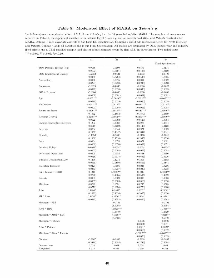
40

Table 5. Moderated Effect of MARA on Tobin’s q Table 5 analyzes the moderated effect of MARA on Tobin’s q for –/+ 10 years before/after MARA. The sample and measures are reported in Table 1, the dependent variable is the natural log of Tobin’s q, and all models hold R&D and Patents constant after MARA. Column 1 adds covariate controls to the basic DD specification. Columns 2 and 3 add interaction terms for R&D Intensity and Patents. Column 4 adds all variables and is our Final Specification. All models are estimated by OLS, include year and industry fixed effects, use a CEM matched sample, and cluster robust standard errors by firm (S.E. in parentheses). Two-tailed tests: ***p<0.01, **p<0.05, *p<0.10.

(1) (2) (3) (4)

Final Specification State Personal Income (log) 0.0186 0.0190 0.0175 0.0174

(0.0197) (0.0191) (0.0196) (0.0190)

State Employment Change -0.2933 -0.0631 -0.2553 -0.0197

(0.8460) (0.8264) (0.8538) (0.8335)

Assets (log) 0.0061 0.0075 0.0007 0.0022

(0.0224) (0.0220) (0.0236) (0.0233)

Employees -0.0029 -0.0036 -0.0016 -0.0022

(0.0029) (0.0028) (0.0030) (0.0029)

SG&A Expense -0.0000 -0.0000 -0.0000 -0.0000

(0.0001) (0.0001) (0.0001) (0.0001)

Age -0.0051** -0.0049** -0.0052*** -0.0050***

(0.0020) (0.0019) (0.0020) (0.0019)

Net Income 0.0013*** 0.0013*** 0.0013*** 0.0013***

(0.0003) (0.0003) (0.0003) (0.0003)

Return on Assets 0.6126*** 0.6988*** 0.6183*** 0.7060***

(0.1862) (0.1853) (0.1870) (0.1859)

Revenue Growth 0.3258*** 0.3063*** 0.3269*** 0.3069***

(0.0522) (0.0562) (0.0523) (0.0564)

Capital Expenditure Intensity 0.4207 0.3908 0.3986 0.3614

(0.3148) (0.3132) (0.3146) (0.3128)

Leverage 0.0864 0.0944 0.0927 0.1009

(0.1053) (0.1047) (0.1044) (0.1041)

Liquidity -0.1096 -0.1300 -0.1110 -0.1318

(0.1530) (0.1510) (0.1535) (0.1516)

Beta 0.0064 0.0074 0.0071 0.0081

(0.0069) (0.0070) (0.0069) (0.0071)

Dividend Policy -0.0004* -0.0004* -0.0004 -0.0004*

(0.0002) (0.0002) (0.0002) (0.0002)

Diversified Operations 0.0301 0.0352 0.0338 0.0396

(0.0636) (0.0618) (0.0633) (0.0616)

Business Combination Law 0.1266 0.1214 0.1213 0.1152

(0.0861) (0.0850) (0.0855) (0.0844)

Patenting Indicator 0.0223 0.0186 0.0244 0.0206

(0.0237) (0.0237) (0.0239) (0.0238)

R&D Intensity (RDI) 0.4210 1.5821*** 0.4039 1.6080***

(0.2726) (0.4365) (0.2595) (0.4389)

Patents 0.0008 0.0009 0.0006 0.0006

(0.0009) (0.0009) (0.0010) (0.0010)

Michigan 0.0729 0.0551 0.0735 0.0565

(0.0773) (0.0858) (0.0770) (0.0860)

After 0.1886* 0.1867* 0.2007* 0.2006**

(0.1032) (0.1016) (0.1025) (0.1010)

MI * After 0.1176* 0.2736** 0.1128* 0.2588**

(0.0645) (0.1283) (0.0630) (0.1262)

Michigan * RDI -0.3101 -0.3703

(1.4703) (1.4584)

After * RDI -1.2826*** -1.3318***

(0.4349) (0.4329)

Michigan * After * RDI 7.5916** 7.2116**

(3.5828) (3.5340)

Michigan * Patents -0.0006 -0.0006

(0.0011) (0.0011)

After * Patents 0.0021* 0.0023*

(0.0013) (0.0012)

Michigan * After * Patents -0.0057*** -0.0055***

(0.0020) (0.0019)

Constant -0.3267 -0.3303 -0.2938 -0.2882

(0.3810) (0.3684) (0.3783) (0.3664)

Observations 3,028 3,028 3,028 3,028 R-squared 0.515 0.524 0.519 0.528

41

Table 6. Predicted values of Tobin’s q Table 6 predicts the outcome value of Tobin’s q in Michigan before MARA, the difference-in-differences (DD) increase of Tobin’s q in Michigan after MARA, and the percentage change of the DD increase. Predictions are based on the Final Specification (Column 4 of Table 5). The Main Effect of MARA (Column 1) is predicted at the 50th percentile of R&D Intensity and Patents, and the mean value of all other predictor variables. Moderator effects are predicted at the 25th and 75th percentiles of each variable so as to not assume normality in their distributions. Due to the skewed distribution in patenting, 48.8% of firms in our sample did not patent at all and so the prediction at the 25th percentile of patents is for firms at Patents = 0. The row “MI before MARA” reports the predicted level of Tobin’s q before MARA. The row “DD Increase” reports the before-to-after difference in the value of Tobin’s q in Michigan after accounting for concurrent changes in comparison states. The row “% Change” reports the predicted DD increase as a percentage of the before period value (i.e. we divide the row labeled “DD Increase” by the row labeled “MI before MARA” and report the result as a percentage).

(1) (2) (3) (4) (5)

Main Effect R&D Intensity Patents

50th

Percentile 25th

Percentile 75th

Percentile No Patents

75th Percentile

MI before MARA 1.29 1.25 1.37 1.29 1.29

DD Increase 0.39 0.07 1.13 0.39 0.34

% Change 30.00% 5.54% 82.40% 30.00% 26.56%

42

Table 7. Robustness Checks of Alternative Comparisons and Placebo Tests Table 7 checks the robustness of the Final Specification (Column 4 of Table 5) to different DD comparisons and placebo tests. All samples follow the same criteria reported in Table 1, the dependent variable is the natural log of Tobin’s q, and R&D and Patents are held constant after MARA. Column 1 restates the Final Specification for ease of comparison. Column 2 compares Michigan to 16 states with a generally low level of non-compete enforcement (i.e., AK AZ CA CO CT HI MT NH NM NY ND OK RI VA WV WI). Column 3 compares Michigan to all other U.S. states. Columns 4-8 test neighboring Midwest states at the time of MARA that did not change their non-compete enforcement level (results are expected to be not significant). All models are estimated by OLS, include year and industry fixed effects, use a CEM matched sample, and cluster robust standard errors by firm (S.E. in parentheses). Two-tailed tests: *** p<0.01, ** p<0.05, * p<0.10.

(1) (2) (3) (4) (5) (6) (7) (8)

Final Spec. Other States All States OH Placebo IN Placebo IL Placebo WI Placebo PA Placebo

State Personal Inc. (log) 0.0174 -0.0143 -0.0068 0.0168 0.0447* 0.0336** -0.0150 0.0219

(0.0190) (0.0173) (0.0105) (0.0189) (0.0264) (0.0165) (0.0198) (0.0180)

State Employment Chg. -0.0197 1.0649* 1.1904*** 0.8099 -0.7748 0.8009 2.4974** 1.8168**

(0.8335) (0.5901) (0.4041) (0.6645) (1.3385) (0.8041) (1.0463) (0.7345)

Assets (log) 0.0022 -0.0148 0.0062 0.0075 0.0259 -0.0311** -0.0135 -0.0024

(0.0233) (0.0172) (0.0098) (0.0192) (0.0364) (0.0150) (0.0203) (0.0151)

Employees -0.0022 -0.0054* -0.0028* 0.0021 0.0068 0.0016* -0.0171*** -0.0003

(0.0029) (0.0028) (0.0016) (0.0021) (0.0043) (0.0009) (0.0041) (0.0013)

SG&A Expense -0.0000 0.0001 0.0002*** -0.0001 -0.0005 -0.0001 0.0005** -0.0000

(0.0001) (0.0001) (0.0001) (0.0001) (0.0003) (0.0001) (0.0002) (0.0000)

Age -0.0050*** -0.0020 -0.0026*** -0.0028 -0.0053 0.0014 -0.0019 -0.0020

(0.0019) (0.0016) (0.0007) (0.0017) (0.0036) (0.0014) (0.0025) (0.0016)

Net Income 0.0013*** -0.0002 0.0003 0.0003* 0.0008 0.0002** 0.0017*** 0.0001

(0.0003) (0.0003) (0.0003) (0.0002) (0.0007) (0.0001) (0.0004) (0.0001)

Return on Assets 0.7060*** 0.5044*** 0.7850*** 0.5362*** 0.7841*** 0.7490*** 0.3221** 0.9314***

(0.1859) (0.1554) (0.1171) (0.1843) (0.2049) (0.1783) (0.1464) (0.1447)

Revenue Growth 0.3069*** 0.2730*** 0.0063 0.2217*** 0.3713*** 0.2383*** 0.3604*** 0.1443***

(0.0564) (0.0385) (0.0061) (0.0378) (0.0615) (0.0388) (0.0482) (0.0517)

Capital Exp. Intensity 0.3614 0.9970*** 1.2610*** 1.1419*** 0.9928*** 0.7982*** 0.6649*** 1.0014***

(0.3128) (0.2675) (0.1382) (0.2475) (0.3029) (0.2571) (0.2410) (0.1833)

Leverage 0.1009 -0.0106 0.0971* -0.0770 0.2510* 0.0527 -0.1209 0.1547**

(0.1041) (0.0897) (0.0528) (0.1021) (0.1279) (0.0865) (0.1046) (0.0691)

Liquidity -0.1318 -0.0647 -0.0144 0.0081 0.2939** -0.1905 -0.2554* -0.0245

(0.1516) (0.1291) (0.0614) (0.1173) (0.1328) (0.1323) (0.1473) (0.1001)

Beta 0.0081 0.0235*** 0.0239*** 0.0157** 0.0002 0.0121* 0.0129* 0.0239***

(0.0071) (0.0058) (0.0038) (0.0073) (0.0090) (0.0068) (0.0070) (0.0049)

Dividend Policy -0.0004* 0.0001 0.0000 0.0533 -0.0009** -0.0009** -0.0006 0.0461

(0.0002) (0.0002) (0.0004) (0.1291) (0.0004) (0.0004) (0.0004) (0.0900)

Diversified Operations 0.0396 -0.0760 -0.0721 -0.0475 -0.0001 -0.0632 -0.1359** -0.0866

(0.0616) (0.0634) (0.0457) (0.0559) (0.0686) (0.0580) (0.0669) (0.0829)

Business Combo Law 0.1152 0.0797* 0.0443* 0.0965 0.1115 0.0791 0.0820 0.0568

(0.0844) (0.0455) (0.0256) (0.0654) (0.0762) (0.0597) (0.0565) (0.0463)

Patenting Indicator 0.0206 0.0055 0.0104 -0.0050 -0.0179 0.0255 -0.0213 -0.0155

(0.0238) (0.0199) (0.0130) (0.0288) (0.0322) (0.0213) (0.0291) (0.0238)

R&D Intensity (RDI) 1.6080*** 2.1567*** 2.2612*** 2.0227*** 1.7213*** 2.7369*** 1.8709*** 1.9477***

(0.4389) (0.4353) (0.2553) (0.3433) (0.5932) (0.3913) (0.4788) (0.3394)

Patents 0.0006 0.0008 -0.0009* -0.0011 -0.0009 0.0002 0.0016 -0.0001

(0.0010) (0.0010) (0.0005) (0.0007) (0.0007) (0.0003) (0.0010) (0.0004)

Michigan 0.0565 0.0657 0.0898 0.0081 0.1291* -0.0150 0.0690 -0.0270

(0.0860) (0.0614) (0.0713) (0.0469) (0.0665) (0.0429) (0.0492) (0.0373)

After 0.2006** 0.3179*** 0.3169*** 0.3786*** 0.1442 0.2931*** 0.3450*** 0.3571***

(0.1010) (0.0659) (0.0385) (0.0837) (0.1472) (0.0784) (0.1076) (0.0730)

MI * After 0.2588** 0.2088** 0.2160** 0.0514 0.0244 0.0079 0.0831 0.0092

(0.1262) (0.1023) (0.1022) (0.0590) (0.0950) (0.0427) (0.1134) (0.0461)

Michigan * RDI -0.3703 0.0923 2.5638 -0.1322 0.4756 0.7559 0.1639 0.8427

(1.4584) (1.4842) (2.2992) (1.3238) (1.6265) (1.5286) (1.1391) (0.8858)

After * RDI -1.3318*** -1.7798*** -1.6213*** -1.9340*** -1.4549** -2.4302*** -1.5626*** -1.7955***

(0.4329) (0.4815) (0.3188) (0.3404) (0.5800) (0.3874) (0.5303) (0.3274)

Michigan * After * RDI 7.2116** 8.5437** 7.3544** -1.2024 -1.0187 0.5100 0.3879 -0.6117

(3.5340) (3.8177) (3.6085) (1.8840) (3.3851) (1.5364) (2.5451) (0.8248)

Michigan * Patents -0.0006 0.0019** 0.0014** 0.0011 -0.0074* -0.0003 -0.0086* 0.0008

(0.0011) (0.0009) (0.0006) (0.0009) (0.0043) (0.0004) (0.0047) (0.0006)

After * Patents 0.0023* 0.0025** 0.0015*** 0.0000 0.0057* 0.0002 0.0002 0.0003

(0.0012) (0.0012) (0.0005) (0.0008) (0.0031) (0.0002) (0.0007) (0.0003)

Michigan * After * Pats. -0.0055*** -0.0053*** -0.0062*** 0.0006 0.0123 0.0001 0.0181 0.0004

(0.0019) (0.0020) (0.0015) (0.0011) (0.0097) (0.0003) (0.0150) (0.0006)

Constant -0.2882 0.3496 0.0692 -0.3440 -1.0655** -0.4260 0.5051 -0.4324

(0.3664) (0.3300) (0.2024) (0.3627) (0.5239) (0.3033) (0.3728) (0.3419)

Observations 3,028 4,668 13,775 4,237 1,753 5,220 2,867 4,468 R-squared 0.528 0.488 0.396 0.554 0.637 0.505 0.619 0.492

43

Table 8. Robustness Checks of Alternative Measures, Specifications and Samples Table 8 checks the robustness of the Final Specification (Column 4 of Table 5) to the selection of different measures, specifications, and samples. The sample and measures are as reported in Table 1 (unless otherwise noted), the dependent variable is the natural log of Tobin’s q, and all models hold R&D and Patents constant after MARA. All of the covariate controls from the Final Specification are included in all models, but are not reported here to conserve space; results for controls are all similar to the Final Specification. Column 1 restates the Final Specification for ease of comparison. Column 2 scales R&D expenses by total assets instead of sales. Column 3 defines Patents as a stock measure that is accumulated and depreciated over 5 prior years. Column 4 defines Patents as equal to the number of inbound patent citations. Column 5 drops year and industry fixed effects. Column 6 defines a new indicator variable (Auto) for the automobile industry and then adds interactions between Auto, Michigan and After to the Final Specification to separately estimate the DD effect of MARA for the automobile industry (the main effect for Auto is collinear with industry fixed effects and is therefore omitted from the analysis). Column 7 expands the sample to include firms that do not report R&D expense by assuming a value of zero for missing data on R&D expenses. Column 8 drops industries with a disproportionate presence in the Michigan economy, including automobiles, transportation equipment, metal products, steel, glass, cement, rubber, plastics, wood and furniture. All models are estimated by OLS, include year and industry fixed effects, use a CEM matched sample, and cluster robust standard errors by firm (S.E. in parentheses). Two-tailed tests: *** p<0.01, ** p<0.05, * p<0.10.

(1) (2) (3) (4) (5) (6) (7) (8) Final

Specification R&D

/Assets Patent Stock

Patent Citations

No Fixed Effects

Auto Interactions

Full Population

Drop Industries

All models include the covariate controls from the Final Specification, but are not reported here to conserve space.

Patenting Indicator 0.0206 0.0170 0.0217 0.0222 -0.0104 0.0199 0.0346* 0.0504 (0.0238) (0.0243) (0.0243) (0.0240) (0.0280) (0.0239) (0.0179) (0.0319) R&D 1.6080*** 1.9259*** 1.6183*** 1.6441*** 2.8728*** 1.6051*** 0.3953*** 0.2373 (0.4389) (0.4529) (0.4420) (0.4399) (0.3923) (0.4389) (0.1274) (0.1502) Patents 0.0006 0.0007 0.0003 0.0000 0.0004 0.0007 -0.0002 0.0018 (0.0010) (0.0010) (0.0004) (0.0001) (0.0009) (0.0010) (0.0004) (0.0019) Michigan (MI) 0.0565 0.0593 0.0553 0.0604 -0.0636 0.0654 0.1157* 0.3400** (0.0860) (0.0840) (0.0848) (0.0871) (0.0747) (0.0917) (0.0628) (0.1435) After 0.2006** 0.2052** 0.1965* 0.2033** 0.0096 0.1982** 0.3468*** 0.4638*** (0.1010) (0.1022) (0.1013) (0.1008) (0.0432) (0.1002) (0.0557) (0.1405) MI * After 0.2588** 0.1643** 0.2413* 0.2513** 0.3439** 0.2646** 0.2356* 0.5597* (0.1262) (0.0832) (0.1241) (0.1256) (0.1503) (0.1277) (0.1306) (0.3202) MI * R&D -0.3703 -0.8396 -0.3881 -0.3731 -0.0596 -0.3194 2.4289** 0.2140 (1.4584) (1.7527) (1.4428) (1.4781) (1.8666) (1.4914) (1.0828) (1.2941) After * R&D -1.3318*** -1.4524*** -1.3198*** -1.4095*** -2.2184*** -1.3261*** -0.2194 0.0542 (0.4329) (0.5456) (0.4419) (0.4274) (0.5013) (0.4346) (0.1464) (0.1330) MI * After * R&D 7.2116** 4.5791* 7.2905** 7.3873** 10.8570*** 8.6370** 3.8595 14.0186 (3.5340) (2.3475) (3.4862) (3.5519) (4.1736) (4.1393) (2.7259) (8.9737) MI * Patents -0.0006 -0.0002 -0.0003 -0.0000 0.0017* -0.0004 0.0002 -0.0013 (0.0011) (0.0012) (0.0004) (0.0001) (0.0009) (0.0011) (0.0004) (0.0042) After * Patents 0.0023* 0.0024** 0.0005 0.0002** 0.0008 0.0022* -0.0006* 0.0044 (0.0012) (0.0012) (0.0004) (0.0001) (0.0012) (0.0012) (0.0003) (0.0040) MI * After * Patents -0.0055*** -0.0061*** -0.0029** -0.0005*** -0.0052*** -0.0054*** -0.0035*** -0.0041 (0.0019) (0.0019) (0.0011) (0.0002) (0.0016) (0.0020) (0.0013) (0.0048) MI * Auto -0.0635 (0.1492) After * Auto 0.0512 (0.0787) MI * After * Auto 0.1273 (0.1476) Constant -0.2882 -0.2848 -0.3218 -0.2728 -0.2257 -0.2920 -0.6441*** 0.0399 (0.3664) (0.3736) (0.3678) (0.3663) (0.3213) (0.3633) (0.2195) (0.0248) Observations 3,028 3,028 3,028 3,028 3,028 3,028 9,208 1,306 R-squared 0.528 0.526 0.526 0.528 0.369 0.528 0.429 0.618

44

Figure 1. Average Tobin’s q for firms in Michigan, compared by industry to firms in comparison states. Figure 1 plots the trend in Tobin’s Q for Michigan and comparison states (AK CA CT MN MT NV ND OK WA WV) for firms that report R&D expense in Compustat. The line labeled “Michigan” is calculated by averaging across industries the separate within-industry averages of Tobin’s q in each year, weighting within-industry averages by individual firm asset size. The line labeled “Comparison Industry” is calculated by averaging across industries in each year the separate within-industry averages of Tobin’s q for those industries that match to a Michigan industry (i.e., omitting industries not represented in Michigan).

11.

52

2.5

3

Aver

age

Tobi

n's

Q1976 1981 1986 1991 1996

Michigan Comparison Industry

45

Figure 2. Predicted difference-in-differences percentage increase in Tobin’s q. Figure 2 graphs the predicted difference-in-differences increase (as a percentage change) in the level of Tobin’s q by percentile of R&D Intensity (along the X axis). The solid (black) line predicts the percentage increase in Tobin’s q for firms that do not patent. The dashed (blue) line predicts the percentage increase in Tobin’s q for firms that patent at the 75th percentile of all patenting firms.

020

4060

80Pr

edic

ted

% in

crea

se in

Tob

in's

q

25 35 45 55 65 75

RDI Percentile

No patenting Patenting at the 75th percentile

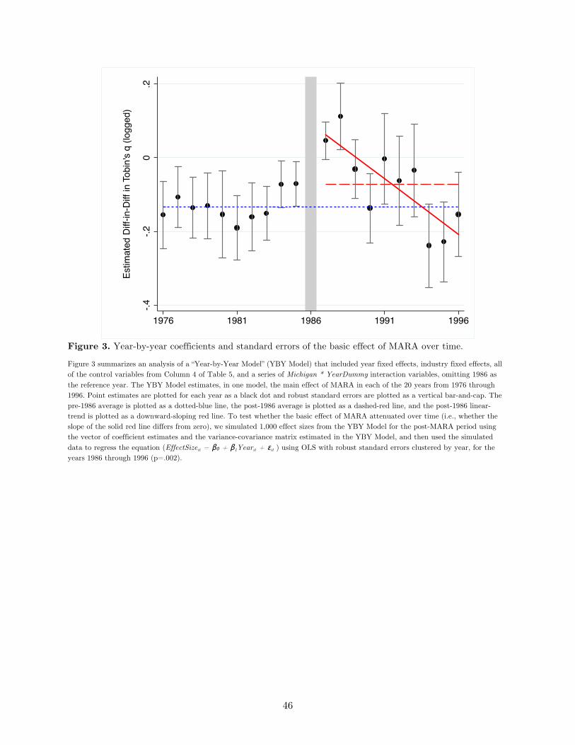
46

Figure 3. Year-by-year coefficients and standard errors of the basic effect of MARA over time. Figure 3 summarizes an analysis of a “Year-by-Year Model” (YBY Model) that included year fixed effects, industry fixed effects, all of the control variables from Column 4 of Table 5, and a series of Michigan * YearDummy interaction variables, omitting 1986 as the reference year. The YBY Model estimates, in one model, the main effect of MARA in each of the 20 years from 1976 through 1996. Point estimates are plotted for each year as a black dot and robust standard errors are plotted as a vertical bar-and-cap. The pre-1986 average is plotted as a dotted-blue line, the post-1986 average is plotted as a dashed-red line, and the post-1986 linear-trend is plotted as a downward-sloping red line. To test whether the basic effect of MARA attenuated over time (i.e., whether the slope of the solid red line differs from zero), we simulated 1,000 effect sizes from the YBY Model for the post-MARA period using the vector of coefficient estimates and the variance-covariance matrix estimated in the YBY Model, and then used the simulated data to regress the equation (EffectSizeit = β0 + β1Yearit + εit ) using OLS with robust standard errors clustered by year, for the years 1986 through 1996 (p=.002).

-.4-.2

0.2

Estim

ated

Diff

-in-D

iff in

Tob

in's

q (lo

gged

)

1976 1981 1986 1991 1996

The Market Value of Knowledge Protection: Evidence from a ...

Documents

Transcript of The Market Value of Knowledge Protection: Evidence from a ...