The Margins of Global Sourcing:

Theory and Evidence from U.S. Firms∗

Pol Antras

Harvard University

and NBER

Teresa C. Fort

Tuck School at Dartmouth

and NBER

Felix Tintelnot

University of Chicago

and NBER

February 8, 2017

Abstract

We develop a quantifiable multi-country sourcing model in which firms self-select into import-

ing based on their productivity and country-specific variables. In contrast to canonical export

models where firm profits are additively separable across destination markets, global sourcing de-

cisions naturally interact through the firm’s cost function. We show that, under an empirically

relevant condition, selection into importing exhibits complementarities across source markets. We

exploit these complementarities to solve the firm’s problem and estimate the model. Comparing

counterfactual predictions to reduced-form evidence highlights the importance of interdependen-

cies in firms’ sourcing decisions across markets, which generate heterogeneous domestic sourcing

responses to trade shocks.

∗Any opinions and conclusions expressed herein are those of the authors and do not necessarily represent the viewsof the U.S. Census Bureau. All results have been reviewed to ensure that no confidential information is disclosed.We are grateful to Treb Allen, Isaiah Andrews, Andy Bernard, Emily Blanchard, Ariel Burstein, Arnaud Costinot,Pablo Fajgelbaum, Paul Grieco, Gene Grossman, Elhanan Helpman, Sam Kortum, Marc Melitz, Eduardo Morales, andMichael Peters for useful conversations, to Andres Rodrıguez-Clare for his comments while discussing the paper at theNBER, to the editor (Penny Goldberg) and two anonymous referees for their constructive comments, and to XiangDing, BooKang Seol and Linh Vu for excellent research assistance. We have also benefited from very useful feedbackfrom seminar audiences at Aarhus, AEA Meetings in Boston, Barcelona GSE, Bank of Spain, Boston College, BostonUniversity, Brown, Cambridge University, Chicago Booth, Dartmouth, ECARES, the Econometric Society Meeting inMinneapolis, ERWIT in Oslo, Harvard, IMF, John Hopkins SAIS, LSE, Michigan, MIT, UQ a Montreal, NationalBank of Belgium, NBER Summer Institute, Northwestern, Princeton, Sciences Po in Paris, SED in Toronto, Stanford,Syracuse, Tsinghua, UBC, UC Berkeley, UC Davis, UC San Diego, Urbana-Champaign, Virginia, and Yale. We thankJim Davis at the Boston RDC for invaluable support with the disclosure process.

1 Introduction

During the last three decades, the world has become increasingly globalized. Dramatic advances

in communication, information, and transportation technologies have revolutionized how and where

firms produce their goods. Intermediate inputs account for approximately two thirds of international

trade (Johnson and Noguera, 2016), and vertical specialization across countries is an important and

growing feature of the world economy (Hummels et al., 2001; Hanson et al., 2005). As global value

chains rise in importance, a firm’s production is more likely than ever to span multiple countries.

There is also mounting evidence that firm-level decisions play a critical role in explaining trade

patterns (Bernard et al., 2009), and that they have important ramifications for aggregate productivity,

employment, and welfare (Goldberg et al., 2010; Hummels et al., 2014).

Despite the growing importance of global production sharing, the canonical model of firm-level

trade decisions (cf. Melitz, 2003) focuses on exporting rather than importing. Since every interna-

tional trade transaction involves an exporter and an importer, a natural question is: can one use the

structure of the well-known exporting framework to analyze firms’ import decisions? Existing export

models cannot be applied directly to analyze foreign sourcing for a simple – yet powerful – reason.

While the canonical export model ensures that a firm’s decision to enter each market can be analyzed

separately by assuming constant marginal costs, a firm chooses to import precisely because it seeks

to lower its marginal costs. In a world in which firm heterogeneity interacts with fixed sourcing costs,

the firm’s decision to import from one market will also affect whether it is optimal to import from

another market. Foreign sourcing decisions are therefore interdependent across markets, making a

model about importing much more complicated to solve theoretically and to estimate empirically.

In this paper, we develop a new framework to analyze firm-level sourcing decisions in a multi-

country world. An important focus of the model is on firms’ extensive margin decisions about which

products to offshore and the countries from which to purchase them. Bernard et al. (2009) find

that these margins account for about 65 percent of the cross-country variation in U.S. imports, and

Bernard et al. (2007) show that U.S. importers are on average more than twice as large and about 12

percent more productive than non-importers.1 In Figure 1, we extend this evidence to show not only

that importers are larger than non-importers, but also that their relative size advantage is increasing

in the number of countries from which they source. The figure indicates that firms that import from

one country are more than twice the size of non-importers, firms that source from 13 countries are

about four log points larger, and firms sourcing from 25 or more countries are over six log points

bigger than non-importers. These importer size advantages are suggestive of sizable country-level

fixed costs of sourcing, which limit the ability of small firms to select into importing from a large

number of countries.2

1We obtain very similar findings when replicating these analyses for the sample of U.S. manufacturing firms used inour empirical analysis (see the Online Appendix, section C.2).

2To construct the figure, we regress the log of firm sales on cumulative dummies for the number of countries fromwhich a firm sources and industry controls. The omitted category is non-importers, so the premia are interpreted as thedifference in size between non-importers and firms that import from at least one country, at least two countries, etc.The horizontal axis denotes the number of countries from which a firm sources, with 1 corresponding to firms that useonly domestic inputs. These premia are robust to controlling for the number of products a firm imports and the numberof products it exports, and thus do not merely capture the fact that larger firms import more products. Consistent with

1

Figure 1: Sales premia and minimum number of sourcing countries in 2007

01

23

45

6P

rem

ium

1 3 5 7 9 11 13 15 17 19 21 23 25Minimum number of countries from which firm sources

Premium 95% CI

Not only do country-level fixed costs of importing appear to be empirically relevant, but they also

seem to be heterogeneous across countries. To illustrate this variation, Table 1 shows the number of

U.S. firms that import from a country versus total sourcing from that country. The table lists the top

ten source countries for U.S. manufacturers in 2007, based on the number of importing firms. These

countries account for 93 percent of importers in our sample and 74 percent of imports. The first

two columns show that Canada ranks number one based on the number of U.S. importers and total

import value. For most other countries, however, country rank based on the number of importers

does not equal the rank based on import values. China is number two for firms but only number three

for value; and Mexico, the number two country in terms of value, ranks eighth in terms of number of

importers.

The considerable divergence between the intensive and extensive margins presented in Table 1

suggests that countries differ not only in terms of their potential as a marginal cost-reducing source

of inputs, but also in terms of the fixed costs firms must incur to import from them. In section 2, we

develop a quantifiable multi-country sourcing model that allows for this possibility. Heterogeneous

firms self-select into importing based on their productivity and country-specific characteristics (wages,

trade costs, and technology). The model delivers a simple closed-form solution for firm profits, in

which marginal costs are decreasing in a firm’s sourcing capability, which is itself a function of the

set of countries from which a firm imports, as well as those countries’ characteristics. Firms can, in

principle, buy intermediate inputs from any country in the world, but acquiring the ability to import

from a country entails a market-specific fixed cost. As a result, relatively unproductive firms may

opt out of importing from high fixed cost countries, even if they are particularly attractive sources of

inputs.

In this environment, the optimality of importing from one country generically depends on the

selection into importing, the same qualitative pattern is also evident among firms that did not import in 2002, and whenusing employment or productivity rather than sales. See section C.3 of the Online Appendix for additional details.

2

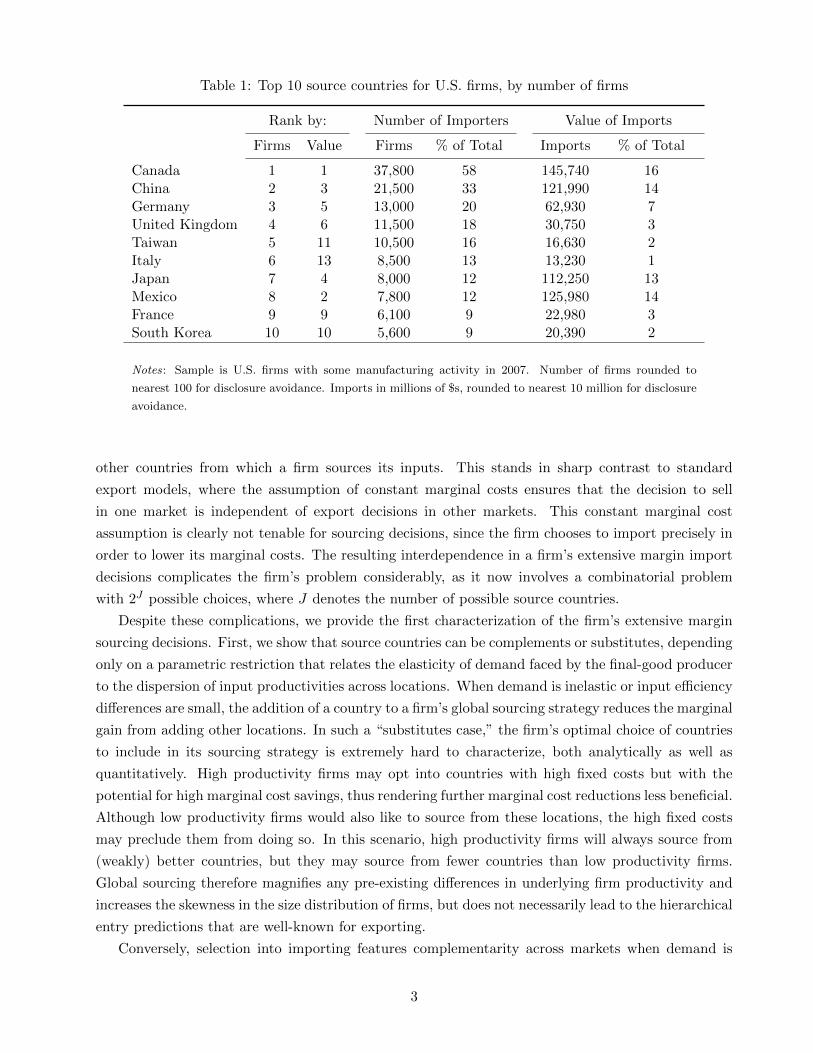
Table 1: Top 10 source countries for U.S. firms, by number of firms

Rank by: Number of Importers Value of Imports

Firms Value Firms % of Total Imports % of Total

Canada 1 1 37,800 58 145,740 16China 2 3 21,500 33 121,990 14Germany 3 5 13,000 20 62,930 7United Kingdom 4 6 11,500 18 30,750 3Taiwan 5 11 10,500 16 16,630 2Italy 6 13 8,500 13 13,230 1Japan 7 4 8,000 12 112,250 13Mexico 8 2 7,800 12 125,980 14France 9 9 6,100 9 22,980 3South Korea 10 10 5,600 9 20,390 2

Notes: Sample is U.S. firms with some manufacturing activity in 2007. Number of firms rounded to

nearest 100 for disclosure avoidance. Imports in millions of $s, rounded to nearest 10 million for disclosure

avoidance.

other countries from which a firm sources its inputs. This stands in sharp contrast to standard

export models, where the assumption of constant marginal costs ensures that the decision to sell

in one market is independent of export decisions in other markets. This constant marginal cost

assumption is clearly not tenable for sourcing decisions, since the firm chooses to import precisely in

order to lower its marginal costs. The resulting interdependence in a firm’s extensive margin import

decisions complicates the firm’s problem considerably, as it now involves a combinatorial problem

with 2J possible choices, where J denotes the number of possible source countries.

Despite these complications, we provide the first characterization of the firm’s extensive margin

sourcing decisions. First, we show that source countries can be complements or substitutes, depending

only on a parametric restriction that relates the elasticity of demand faced by the final-good producer

to the dispersion of input productivities across locations. When demand is inelastic or input efficiency

differences are small, the addition of a country to a firm’s global sourcing strategy reduces the marginal

gain from adding other locations. In such a “substitutes case,” the firm’s optimal choice of countries

to include in its sourcing strategy is extremely hard to characterize, both analytically as well as

quantitatively. High productivity firms may opt into countries with high fixed costs but with the

potential for high marginal cost savings, thus rendering further marginal cost reductions less beneficial.

Although low productivity firms would also like to source from these locations, the high fixed costs

may preclude them from doing so. In this scenario, high productivity firms will always source from

(weakly) better countries, but they may source from fewer countries than low productivity firms.

Global sourcing therefore magnifies any pre-existing differences in underlying firm productivity and

increases the skewness in the size distribution of firms, but does not necessarily lead to the hierarchical

entry predictions that are well-known for exporting.

Conversely, selection into importing features complementarity across markets when demand is

3

relatively elastic (so profits are particularly responsive to variable cost reductions) and input efficiency

levels are relatively heterogeneous across markets (so that the reduction in expected costs from adding

an extra country in the set of active locations is relatively high). This case is much more tractable,

and delivers sharp results rationalizing the monotonicity in the sales premia observed in Figure 1. In

particular, we use standard tools from the monotone comparative statics literature to show that, in

such a case, the sourcing strategies of firms follow a strict hierarchical structure in which the number

of countries in a firm’s sourcing strategy increases (weakly) with the firm’s core productivity level.3

Our quantitative analysis enables separate identification of the sourcing potential of a country

– a function of technology, trade costs, and wages capturing the potential of a country as source

of marginal cost savings – and the fixed cost of sourcing from that country. We use 2007 Census

data on U.S. manufacturers’ mark-ups and import shares to recover the sourcing potential of 66

foreign countries, as well as the average elasticity of demand and dispersion of input productivities

faced by U.S. firms. Consistent with the pattern documented in Figure 1, we find robust evidence

suggesting that the extensive margin sourcing decisions of U.S. firms are complements. This finding

paves the way for an additional methodological contribution of our paper –namely, to solve the firm’s

problem and estimate the model structurally. To do so, we apply an iterative algorithm developed

by Jia (2008), which exploits the complementarities in the ‘entry’ decisions of firms, and uses lattice

theory to reduce the dimensionality of the firm’s optimal sourcing strategy problem. We can therefore

estimate the fixed costs of sourcing, which range from a median of 10,000 to 56,000 USD, are around

13 percent lower for countries with a common language, and increase in distance with an elasticity

of 0.19. In line with the premise that countries differ along two dimensions, the relative rankings of

these fixed costs are also quite different from the rankings of countries’ potential to reduce marginal

costs.

The structural estimation of the model is informative not only because it shows the importance

of marginal cost savings versus fixed cost heterogeneity across countries, but also because it allows

for counterfactual exercises.4 We exploit this capability by studying the implications of an increase

in China’s sourcing potential calibrated to match the observed growth in the share of U.S. firms

importing from China between 1997 and 2007. These years are governed both by data availability,

and the fact that they span China’s accession to the World Trade Organization (WTO). Consistent

with other quantitative models of trade, the China shock increases the competitive environment by

decreasing the equilibrium industry-level U.S. price index and driving some U.S. final good producers

out of the market. Although the net result of these forces is a marked decrease in domestic sourcing

(and U.S. employment) in that sector, the net decline masks significant heterogeneity in how the shock

affects the sourcing decisions of firms at different points in the size distribution. More specifically, the

shock induces a range of U.S. firms to select into sourcing from China, and on average, these firms

increase their input purchases not only from China, but also from the U.S. and other countries. The

3The seminal applications of the mathematics of complementarity in the economics literature are Vives (1990) andMilgrom and Roberts (1990). Grossman and Maggi (2000) and Costinot (2009) are particularly influential applicationsof these techniques in international trade environments.

4This is in contrast to moment inequality methods, which were first adopted in an international trade context byMorales et al. (2014).

4

existence of gross changes in sourcing that operate in different directions is a distinctive feature of our

framework that does not arise in the absence of fixed costs of offshoring or whenever entry decisions

are independent across markets.

To assess the empirical relevance of these channels, we compare the model’s counterfactual pre-

dictions to the observed changes in U.S. manufacturers’ sourcing from the U.S. and third markets

between 1997 and 2007. We first show that the same qualitative patterns predicted by the model are

evident in the raw data. Firms that begin importing from China over this period grow their domestic

and third market sourcing the most, continuing importers have smaller but still positive sourcing

changes, and firms that never import from China shrink their domestic sourcing and increase third-

market sourcing by a substantially smaller amount than both new and continuing China importers.

To ensure that the patterns observed in the raw data are not driven solely by firm-specific demand or

productivity shocks, we construct an exogenous firm-level shock to Chinese sourcing potential in the

spirit of Autor et al. (2013) and Hummels et al. (2014). The results show that exogenous increases

in firm-level imports from China do not decrease domestic and third market sourcing –as might be

expected in a world with no interdependencies in sourcing decisions– but instead are associated with

increased firm-level sourcing from other markets. We thus provide both structural and reduced-form

evidence of the empirical relevance of interdependencies in firms’ extensive margin import decisions.

Our paper contributes to three distinct literatures. First, we add to a large body of theoretical

work on foreign sourcing. We follow existing theory that adapts the Melitz (2003) model to char-

acterize heterogeneous firms’ foreign sourcing decisions (e.g., Antras and Helpman, 2004, 2008), but

our framework also shares features with a parallel literature that uses the Eaton and Kortum (2002)

model to study offshoring (Rodrıguez-Clare, 2010; Garetto, 2013). More specifically, we build on the

approach in Tintelnot (forthcoming) of embedding the Eaton and Kortum (2002) stochastic represen-

tation of technology into the problem of a firm, though in our context firms choose optimal sourcing

rather than final-good production locations. This approach allows us to move beyond the two-country

frameworks that have pervaded the literature and develop a tractable multi-country model. A key

theoretical insight from our model is that a positive shock to sourcing from one location could lead a

firm either to decrease its sourcing from other locations as it substitutes away from them, or instead

to grow sufficiently so that it increases its net sourcing from other locations. This prediction is remi-

niscent of Grossman and Rossi-Hansberg (2008), who show that an offshoring industry may expand

domestic employment if a “productivity effect” dominates a “substitution effect.” An important

difference is that in our framework, these effects take place within a firm rather than an industry.

Our paper also relates to an extensive empirical literature on offshoring. A number of papers

provide reduced form evidence on the determinants of offshoring (Fort, forthcoming), as well as its

impact on firm performance and aggregate productivity (Amiti and Konings, 2007; Goldberg et al.,

2010; De Loecker et al., 2016). A related set of papers uses a more structural approach to quantify

the effect of importing on firm productivity and prices (Halpern et al., 2015; Gopinath and Neiman,

2014; Blaum et al., 2015). The first part of our estimation provides a similar quantification, implying

that a firm sourcing from all foreign countries faces nine percent lower variable costs and achieves 32

5

percent higher sales than when sourcing exclusively from domestic suppliers.5 The most important

distinction between those papers and ours is that we provide evidence not just on the intensive margin

implications of importing, but also on the firm’s extensive margin sourcing decisions in a multi-country

setting with heterogeneous fixed costs across countries. While Blaum et al. (2013) discuss the existence

of interdependencies across sourcing decisions in a model with an arbitrary number of countries and

inputs, ours is the first paper to characterize the extensive margin of importing in this setting and to

solve the firm’s problem quantitatively.

Finally, we contribute to a growing body of work that analyzes interdependencies in firm-level

decisions. Yeaple (2003) and Grossman et al. (2006) first described the inherent difficulties in solving

for the extensive margin of imports in a multi-country model with multiple intermediate inputs and

heterogeneous fixed costs of sourcing. Those authors obtained partial characterizations of the problem

in models with at most three countries and two inputs. We provide the first characterization of the

firm’s extensive margin sourcing decision in this setting with multiple inputs and countries, and

show how these decisions can be aggregated to describe trade flows across countries. These trade

flow equations collapse to the well-known Eaton and Kortum (2002) gravity equation whenever fixed

costs are zero (so that there is universal importing), or to the Chaney (2008) gravity equation in the

knife-edge case that shuts down interdependencies across markets. In a general setting, our model

delivers an extended gravity equation reminiscent of Morales et al. (2014), who estimate a model with

interdependencies in firms’ export decisions. That paper uses moment inequalities to partially identify

the cost parameters and does not conduct any counterfactual analysis. Tintelnot (forthcoming) solves

the optimal plant location problem of multinational firms in a general equilibrium model, however,

in a setting with much fewer countries. We overcome the challenges in prior work by combining

the theoretical insights on complementarity with Jia’s (2008) algorithm for solving Walmart’s and

Kmart’s decisions about whether and where to open new retail establishments. Our paper is the first

to adopt this algorithm in an international setting or in a setting with more than two firms.

The rest of the paper is structured as follows. We present the assumptions of our model in section

2 and solve for the equilibrium in section 3. In section 4, we introduce the data and provide descriptive

evidence supporting the assumptions underlying our theoretical framework. We estimate the model

structurally in section 5, and in section 6, we perform our counterfactual analysis and compare the

predictions of the model to reduced-form evidence. Section 7 concludes.

2 Theoretical Framework

In this section, we develop our quantifiable multi-country model of global sourcing.

5Quantitatively, this is lower than the findings of Halpern et al. (2015) for Hungarian firms. Using a two-countrymodel and a method similar to Olley and Pakes (1996), they find that importing all foreign varieties would increaseproductivity of a Hungarian firm by 22 percent. Blaum et al. (2015) obtain even larger cost reduction estimates forsome French firms, perhaps due to an alternative interpretation of idiosyncratic differences in sourcing shares (e.g., asmeasurement error in our context and as structural error in their paper).

6

2.1 Preferences and Endowments

Consider a world consisting of J countries in which individuals value the consumption of differentiated

varieties of manufactured goods according to a standard symmetric CES aggregator

UMi =

∫ω∈Ωi

qi (ω)(σ−1)/σ dω

σ/(σ−1)

, σ > 1, (1)

where Ωi is the set of manufacturing varieties available to consumers in country i ∈ J (with some

abuse of notation we denote by J both the number as well as the set of countries; we use subscripts

i and j to denote countries). These preferences are assumed to be common worldwide and give rise

to the following demand for variety ω in country i:

qi (ω) = EiPσ−1i pi (ω)−σ , (2)

where pi (ω) is the price of variety ω, Pi is the standard ideal price index associated with (1), and

Ei is aggregate spending on manufacturing goods in country i. For what follows it will be useful to

define a (manufacturing) market demand term for market i as:

Bi =1

σ

(σ

σ − 1

)1−σEiP

σ−1i . (3)

There is a unique factor of production, labor, which commands a wage wi in country i. When

we close the model in general equilibrium, we later introduce a freely tradable, non-manufacturing

sector into the economy. This non-manufacturing sector captures a constant share of the economy’s

spending, also employs labor, and is large enough to pin down wages in terms of that ‘outside’ sector’s

output.

2.2 Technology and Market Structure

There exists a measure Ni of final-good producers in each country i ∈ J , and each of these produc-

ers owns a blueprint to produce a single differentiated variety. The market structure of final good

production is characterized by monopolistic competition, and there is free entry into the industry.

Production of final-good varieties requires the assembly of a bundle of intermediates. We index

final-good firms by their ‘core productivity’, which we denote by ϕ, and which governs the mapping

between the bundle of inputs and final-good production. Following Melitz (2003), we assume that

firms only learn their productivity ϕ after incurring an entry cost equal to fei units of labor in country

i. This core productivity is drawn from a country-specific distribution gi (ϕ), with support in [ϕi,∞),

and with an associated continuous cumulative distribution Gi (ϕ). For simplicity, we assume that

final-good varieties are prohibitively costly to trade across borders.

Intermediates can instead be traded internationally, and a key feature of the equilibrium will

be determining the location of production of different intermediates. The bundle of intermediates

contains a continuum of measure one of firm-specific inputs, assumed to be imperfectly substitutable

7

with each other, with a constant and symmetric elasticity of substitution equal to ρ. Very little

will depend on the particular value of ρ. All intermediates are produced with labor under constant-

returns-to-scale technologies. We denote by aj (v, ϕ) the unit labor requirement associated with the

production of firm ϕ’s intermediate v ∈ [0, 1] in country j ∈ J .

Although intermediates are produced worldwide, a final-good producer based in country i only

acquires the capability to offshore in j after incurring a fixed cost equal to fij units of labor in country

i. We denote by Ji (ϕ) ⊆ J the set of countries for which a firm based in i with productivity ϕ has

paid the associated fixed cost of offshoring wifij . For brevity, we will often refer to Ji (ϕ) as the

global sourcing strategy of that firm.

Intermediates are produced by a competitive fringe of suppliers who sell their products at marginal

cost.6 Shipping intermediates from country j to country i entails iceberg trade costs τij . As a result,

the cost at which firms from i can procure input v from country j is given by τijaj (v, ϕ)wj , and the

price that firm ϕ based in country i pays for input v can be denoted by

zi (v, ϕ;Ji (ϕ)) = minj∈Ji(ϕ)

τijaj (v, ϕ)wj . (4)

We can then express the marginal cost for firm ϕ based in country i of producing a unit of a

final-good variety as

ci (ϕ) =1

ϕ

(∫ 1

0zi (v, ϕ;Ji (ϕ))1−ρ dv

)1/(1−ρ)

. (5)

Building on Eaton and Kortum (2002), we treat the (infinite-dimensional) vectors of firm-specific

intermediate input efficiencies 1/aj (v, ϕ) as the realization of an extreme value distribution. More

specifically, suppliers in j draw the value of 1/aj (v, ϕ) from the Frechet distribution

Pr(aj (v, ϕ) ≥ a) = e−Tjaθ, with Tj > 0. (6)

These draws are assumed to be independent across locations and inputs. As in Eaton and Kortum

(2002), Tj governs the state of technology in country j, while θ determines the variability of produc-

tivity draws across inputs, with a lower θ fostering the emergence of comparative advantage within

the range of intermediates across countries.

2.3 Discussion of Assumptions

This completes the description of the key assumptions of the model. A number of dimensions of

our setup are worth discussing. First, although we have assumed that inputs are firm-specific, our

model is in fact isomorphic to one in which the unit measure of inputs, as well as their associated

unit labor requirements aj (v, ϕ), are identical for all firms and denoted by aj (v). We emphasize the

firm-specificity of inputs to justify why intermediaries (e.g., wholesalers) would not trivially eliminate

the need for all firms to incur fixed costs of foreign sourcing. Second, to highlight the importance of

importing, we have assumed that final-good varieties cannot be traded across borders. In the Online

6Implicitly, we assume that contracts between final-good producers and suppliers are perfectly enforceable, so thatthe firm-specificity of inputs is irrelevant for the prices at which inputs are transacted.

8

Appendix (section B.3), we relax this assumption and study the joint determination of the extensive

margins of both exports and imports, an approach that has been further pursued by Bernard et al.

(2016). Third, our model assumes that all final-good producers combine a measure one of inputs in

production. As we demonstrate in the Online Appendix (section B.3), it is simple to generalize our

framework to the case in which final-good producers also hire local labor to assemble the bundle of

inputs, and in which firms optimally choose the complexity of production, as captured by the measure

of inputs used in production (see Acemoglu et al., 2007). The qualitative results of these extensions

are analogous to those of our benchmark model, but incorporating these features would significantly

complicate the structural estimation. Fourth, tractability concerns also dictate our assumption that

wages are pinned down in a non-manufacturing sector, as we discuss at greater length in section

6. Finally, we have introduced an asymmetric market structure in the final- and intermediate-input

sectors because this allows our model to nest two key workhorse trade models developed in recent

years. It would be feasible to turn the intermediate-input sector into a monopolistically competitive

sector with a fixed mass of firms, and the relevant expressions would all be very similar.

3 Equilibrium

We solve for the equilibrium of the model in three steps. First, we describe optimal firm behavior

conditional on a given sourcing strategy Ji (ϕ). Second, we characterize the choice of this sourcing

strategy and relate our results to some of the stylized facts discussed in the Introduction. Third, we

aggregate the firm-level decisions and solve for the general equilibrium of the model. We conclude

this section by outlining the implications of our framework for bilateral trade flows across countries.

3.1 Firm Behavior Conditional on a Sourcing Strategy

Consider a firm based in country i with productivity ϕ that has incurred all fixed costs associated

with a given sourcing strategy Ji (ϕ). In light of the cost function in (5), it is clear that after learning

the vector of unit labor requirements for each country j ∈ Ji (ϕ), the firm will choose the location

of production for each input v that solves minj∈Ji(ϕ) τijaj (v, ϕ)wj. Using the properties of the

Frechet distribution in (6), one can show that the firm will source a positive measure of intermediates

from each country in its sourcing strategy set Ji (ϕ). Furthermore, the share of intermediate input

purchases sourced from any country j (including the home country i) is simply given by

χij (ϕ) =Tj (τijwj)

−θ

Θi (ϕ)if j ∈ Ji (ϕ) (7)

and χij (ϕ) = 0 otherwise, where

Θi (ϕ) ≡∑

k∈Ji(ϕ)

Tk (τikwk)−θ . (8)

The term Θi (ϕ) summarizes the sourcing capability of firm ϕ from i. Note that, in equation (7),

each country j’s market share in the firm’s purchases of intermediates corresponds to this country’s

9

contribution to its sourcing capability Θi (ϕ). Countries in the set Ji (ϕ) with lower wages wj , more

advanced technologies Tj , or lower trade costs when selling to country i will have higher market

shares in the intermediate input purchases of firms based in country i. We shall refer to the term

Tj (τijwj)−θ as the sourcing potential of country j from the point of view of firms in i.7

After choosing the least cost source of supply for each input v, the overall marginal cost faced by

firm ϕ from i can be expressed, after some cumbersome derivations, as

ci (ϕ) =1

ϕ(γΘi (ϕ))−1/θ , (9)

where γ =[Γ(θ+1−ρθ

)]θ/(1−ρ)and Γ is the gamma function.8 Note that in light of equation (8), the

addition of a new location to the set Ji (ϕ) increases the sourcing capability of the firm and necessarily

lowers its effective marginal cost. Intuitively, an extra location grants the firm an additional cost draw

for all varieties v ∈ [0, 1], and it is thus natural that this greater competition among suppliers will

reduce the expected minimum sourcing cost per intermediate. In fact, the addition of a country to

Ji (ϕ) lowers the expected price paid for all varieties v, and not just for those that are ultimately

sourced from the country being added to Ji (ϕ).

Using the demand equation (2) and the derived marginal cost function in (9), we can express the

firm’s profits conditional on a sourcing strategy Ji (ϕ) as

πi (ϕ) = ϕσ−1 (γΘi (ϕ))(σ−1)/θ Bi − wi∑

j∈Ji(ϕ)

fij , (10)

where Bi is given in (3). As is clear from equation (10), when deciding whether to add a new country

j to the set Ji (ϕ), the firm trades off the reduction in costs associated with the inclusion of that

country in the set Ji (ϕ) – which increases the sourcing capability Θi (ϕ) – against the payment of

the additional fixed cost wifij .

It is worth highlighting the connection between our modeling of the gains from importing interme-

diate inputs and the Armington-style approach that is standard in the literature on importing.9 More

specifically, suppose that all suppliers in a given country produce the same intermediate input using

local labor under a constant-returns-to-scale technology featuring a unit labor requirement equal to

(γTj)−1/θ in each country j ∈ J . Assume, in addition, that inputs are differentiated by country of

origin with an elasticity of substitution across inputs from any two locations equal to 1 + θ. Finally,

as in our framework, assume that in order to import country j’s unique input, final-good producers

in i need to incur a fixed costs equal to wifij and iceberg trade costs τij . Under these assumptions, it

is then straightforward to verify that the resulting firm profits will be identical to those in equation

7It may seem surprising that the dependence of country j’s market share χij (ϕ) on wages and trade costs is shapedby the Frechet parameter θ and not by the substitutability across inputs, as governed by the parameter ρ in equation(5). The reason for this, as in Eaton and Kortum (2002), is that variation in market shares is explained exclusively bya product-level extensive margin.

8These derivations are analogous to those performed by Eaton and Kortum (2002) to solve for the aggregate priceindex in their model. To ensure a well-defined marginal cost index, we assume θ > ρ − 1. Apart from satisfying thisrestriction, the value of ρ does not matter for any outcomes of interest and will be absorbed into a constant.

9See, among others, Halpern et al. (2015), Goldberg et al. (2010), and Gopinath and Neiman (2014).

10

(10) above.

This isomorphism between our model and the love-for-variety approach carries three significant

implications. First, it should be clear that the interdependencies in the firm’s extensive margin sourc-

ing decisions are also a feature of the Armington-style models that have pervaded the literature on

importing. Second, it follows that the results below on the optimal determination of the sourcing

strategy Ji (ϕ), as well as the techniques we develop in section 5 to structurally estimate the model,

are also applicable in these types of models. Third, it implies that our model provides an intuitive mi-

crofoundation for why being able to import from (several) foreign countries is productivity-enhancing,

without resorting to the elusive notion of input differentiation by country of origin. With this in mind,

we next turn to an analysis of the optimal sourcing strategy of firms.

3.2 Optimal Sourcing Strategy

Each firm’s optimal sourcing strategy is a combinatorial optimization problem in which a set Ji (ϕ) ⊆J of locations is chosen to maximize the firm’s profits πi (ϕ) in (10). We can alternatively express

this problem as

maxIij∈0,1Jj=1

πi (ϕ, Ii1, Ii2, ..., IiJ) = ϕσ−1

γ J∑j=1

IijTj (τijwj)−θ

(σ−1)/θ

Bi − wiJ∑j=1

Iijfij , (11)

where the indicator variable Iij takes a value of 1 when j ∈ Ji (ϕ), and 0 otherwise. The problem

in (11) is not straightforward to solve because the decision to include a country j in the set Ji (ϕ)

depends on the number and characteristics of the other countries in this set. In theory, one could

simply calculate firm profits for different combinations of locations and pick the unique strategy

yielding the highest level of profits. In practice, however, this would amount to computing profits

for 2J possible strategies, which is clearly infeasible unless one chooses a small enough number J of

candidate countries.

Inspection of (11) reveals, however, that the profit function πi is supermodular in ϕ and Θi (ϕ),

and features increasing differences in (Iij , Iik) for j, k ∈ 1, ..., J and j 6= k, whenever (σ − 1) /θ >

1. These properties of the problem in (11) allow us to establish the following result (the proof is

straightforward and is relegated to the Online Appendix):

Proposition 1. The solution Iij (ϕ) ∈ 0, 1Jj=1 to the optimal sourcing problem (11) is such that:

(a) a firm’s sourcing capability Θi (ϕ) =J∑j=1

Iij (ϕ)Tj (τijwj)−θ is nondecreasing in ϕ;

(b) if (σ − 1) /θ ≥ 1, then Ji (ϕL) ⊆ Ji (ϕH) for ϕH ≥ ϕL, where Ji (ϕ) = j : Iij (ϕ) = 1.

Part (a) of Proposition 1 simply states that more productive firms choose a larger sourcing ca-

pability –either because they select into more countries or because they select into better countries–

thereby magnifying their cost advantage relative to less productive firms. This in turn implies that

the equilibrium size distribution of firms will feature more positive skewness than what would be

observed without foreign sourcing.

11

It is important to emphasize that this first result does not imply that the extensive margin of

sourcing at the firm level (i.e., the number of elements of Ji (ϕ)) is necessarily increasing in firm

productivity as well. For example, a highly productive firm from i might pay a large fixed cost to

offshore to a country j∗ with a particularly high sourcing potential (i.e., a high value of Tj∗ (τij∗wj∗)−θ)

– thus greatly increasing Θi – after which the firm might not have an incentive to add further locations

to its sourcing strategy. Instead, a low productivity firm from i might not be able to profitably offshore

to j∗, but may well find it optimal to source from two foreign countries with associated lower fixed

costs.

Part (b) of Proposition 1 states, however, that this possibility can only arise when (σ − 1) /θ < 1.

When instead (σ − 1) /θ ≥ 1, the cardinality of the set Ji (ϕ) is necessarily weakly increasing in ϕ.

Because firm size is increasing in core productivity ϕ, this prediction is consistent with the upward

sloping sales premium documented in Figure 1 in the Introduction. The intuition behind this second

result in Proposition 1 rests on the fact that, when (σ − 1) /θ > 1, the profit function πi (ϕ) features

increasing differences in (Iij , Iik) for j, k ∈ 1, ..., J and j 6= k, and thus the marginal gain from adding

a new location to the set Ji (ϕ) cannot possibly be reduced by the addition of other countries to the

set. This case is more likely to apply whenever demand is elastic and thus profits are particularly

responsive to variable cost reductions (high σ), and whenever input efficiency levels are relatively

heterogeneous across markets (low θ), so that one achieves a relatively high reduction of costs by

adding an extra country into the set of active locations.10

Part (b) of Proposition 1 also has the strong implication that there should be a strict hierarchical

order in the extensive margin of offshoring – a ‘pecking order’ which is reminiscent of the one typically

obtained in models of exporting with heterogeneous firms, such as Eaton et al. (2011). This prediction

is very strong and often violated in the data: it is not uncommon to observe less productive firms

sourcing from countries from which more productive firms do not source. Still, in section 4.2 we show

that 36 percent of U.S. firms follow the predicted pecking order from the top ten source countries,

whereas we would expect only 20 percent to do so if the probabilities to source from individual

countries were independent and equal to the share of importers that source from them.

A possible explanation for the violation of a strict hierarchy of import sources is the fact that fixed

costs of sourcing might be heterogeneous across firms. With that in mind, our structural estimation

in section 5 will incorporate such heterogeneity in fixed costs. In that section, a variant of part (b) of

Proposition 1 will be instrumental for reducing the dimensionality of the optimal sourcing problem.

In particular, because of increasing differences in the profit function when σ − 1 > θ, we can state

(see the Online Appendix for a formal proof):

Proposition 2. For all j ∈ 1, ..., J, define the mapping Vi,j(ϕ,J ) to take a value of one whenever

including country j in the sourcing strategy J raises firm-level profits πi (ϕ,J ) , and to take a value

of zero otherwise. Then, whenever (σ − 1) /θ ≥ 1, Vi,j(ϕ,J ′) ≥ Vi,j(ϕ,J ) for J ⊆ J ′.

The usefulness of this result is best demonstrated with an example. Suppose that one is trying

10Readers familiar with the work of Eaton and Kortum (2002) might expect that θ > σ − 1 is in fact implied by theneed for the firm’s marginal cost function to be well-defined. Note, however, that our parameter ρ plays the role of σin the Eaton-Kortum setup, and thus this technical condition is instead θ > ρ− 1 in our setup (see footnote 8).

12

to assess whether a given country j belongs in the firm’s optimal sourcing strategy Ji (ϕ). Without

guidance from the theory, one would need to compute all 2J candidate sourcing strategies to answer

that question. Proposition 2 implies, however, that if for country j, Vi,j(ϕ,J ) = 1 when J is the

null set, then j is necessarily in Ji (ϕ), while if Vi,j(ϕ,J ) = 0 when J includes all countries except

for j, then j cannot possibly be in Ji (ϕ). In section 5 we will discuss Jia’s (2008) algorithm, which

leverages this logic to devise an iterative algorithm to solve the problem defined in (11) efficiently.

In our above discussion, we have focused on the ‘complements case’ (σ− 1 > θ), which allows one

to characterize some key properties of the optimal sourcing problem in (11) without any restriction

on the relationship between the various countries’ sourcing potentials and fixed costs of sourcing.

In the ‘substitutes case’ (σ − 1 < θ), this is no longer feasible and one needs to make additional

assumptions to obtain a sharp characterization of the firm’s sourcing strategy. For instance, consider

a situation in which the fixed costs of offshoring are common for all foreign countries (as in Blaum

et al., 2015), so fij = fiO for all j 6= i. In such a case, and regardless of the value of (σ − 1) /θ, one

could then rank foreign locations j 6= i according to their sourcing potential Tj (τijwj)−θ and denote

by ir = i1, i2,..., iJ−1 the country with the r-th highest value of Tj (τijwj)−θ. Having constructed

ir, it then follows that for any firm with productivity ϕ from i that offshores to at least one country,

we have i1 ∈ Ji (ϕ); for any firm that offshores to at least two countries, we have i2 ∈ Ji (ϕ); and so

on. In other words, not only does the extensive margin increase monotonically with firm productivity,

but it does so in a manner uniquely determined by the ranking of the Tj (τijwj)−θ sourcing potential

terms. It is important to emphasize, however, that this result relies on the assumption of identical

offshoring fixed costs across sourcing countries, an assumption that appears particularly unlikely in

light of the evidence documented in Table 1.

Even in the presence of cross-country differences in the fixed costs of offshoring, a similar sharp

result emerges in the knife-edge case in which (σ − 1) /θ = 1. In that case, the addition of an

element to the set Ji (ϕ) has no effect on the decision to add any other element to the set, and the

same pecking order pattern described in the previous paragraph applies, but when one ranks foreign

locations according to the ratio Tj (τijwj)−θ /fij rather than Tj (τijwj)

−θ. This result is analogous to

the one obtained in standard models of selection into exporting featuring constant marginal costs, in

which the decision to service a given market is independent of that same decision in other markets.

We close this section by using the properties of the profit function to discuss comparative statics

that apply when holding constant the market demand level Bi. First, and quite naturally, a reduction

in any iceberg trade cost τij or fixed cost of sourcing fij (weakly) increases the firm’s sourcing

capability Θi (ϕ) and thus firm-level profits. Second, in the complements case, a reduction of any τij

or fij also (weakly) increases the extensive margin of global sourcing, in the sense that the set Ji (ϕ)

is nondecreasing in τij and fij for any j. Third, and perhaps more surprisingly, in the complements

case a reduction of any τij or fij (weakly) increases firm-level bilateral input purchases from all

countries. To see this, note that firm-level intermediate input purchases from any country j ∈ Ji (ϕ)

are a fraction (σ − 1)χij (ϕ) of firm profits, and using (7) and (10), they can thus be expressed as

13

Mij (ϕ) =

(σ − 1)Biγ(σ−1)/θϕσ−1 (Θi (ϕ))(σ−1−θ)/θ Tj (τijwj)

−θ if j ∈ Ji (ϕ)

0 otherwise.(12)

When (σ − 1) /θ ≥ 1, Mij (ϕ) is thus increasing in all the terms in Θi (ϕ). Intuitively, when

demand is sufficiently elastic (i.e., σ is high enough) or the strength of comparative advantage in the

intermediate-good sector across countries is sufficiently high (i.e., θ is low enough), the scale effect

through the demand response to lower costs dominates the direct substitution effect related to market

shares shifting towards the locations whose costs of sourcing have been reduced. It is useful to restate

this third result in the following way (see the Online Appendix for a formal proof):

Proposition 3. Holding constant the market demand level Bi, whenever (σ − 1) /θ ≥ 1, an increase

in the sourcing potential Tj (τijwj)−θ or a reduction in the fixed cost fj of any country j, (weakly)

increases the input purchases by firms in i not only from j, but also from all other countries.

It should be emphasized that the sharp results above only apply when holding market demand –

of which the price index is a key component – fixed. In general equilibrium, these same parameters

also affect the level of market demand. As we shall see in our counterfactual exercise in section 6,

the endogenous response of market demand is quantitatively important in our estimation, and thus

the implications we derive from changes in trade costs are much more nuanced than those discussed

above (see Bache and Laugesen, 2013). Despite these nuances, Proposition 3 will still prove to be very

useful in interpreting our counterfactual results and in relating them to the observed transformation

in the global sourcing practices of U.S. firms over the period 1997-2007.

3.3 Industry and General Equilibrium

Consider now the general equilibrium of the model. As mentioned before, we simplify matters by

assuming that consumers spend a constant share (which we denote by η) of their income on manufac-

turing. The remaining share 1 − η of income is spent on a perfectly competitive non-manufacturing

sector that competes for labor with manufacturing firms. Technology in that sector is linear in labor,

and we assume that 1−η is large enough to guarantee that the wage rate wi in each country i is pinned

down by labor productivity in that sector. For simplicity, we also assume that this ‘outside’ sector’s

output is homogeneous, freely tradable across countries, and serves as a numeraire in the model. We

thus can treat wages as exogenous in solving for the equilibrium in each country’s manufacturing

sector.

We next turn to describing the equilibrium in the manufacturing sector. Given our assumption

that final-good producers only observe their productivity after paying the fixed cost of entry, we can

use equation (10) to express the free-entry condition in manufacturing as

∫ ∞ϕi

ϕσ−1 (γΘi (ϕ))(σ−1)/θ Bi − wi∑

j∈Ji(ϕ)

fij

dGi (ϕ) = wifei. (13)

14

In the lower bound of the integral, ϕi denotes the productivity of the least productive active firm

in country i. Firms with productivity ϕ < ϕi cannot profitably source from any country and thus

exit upon observing their productivity level. Note that Bi affects expected operating profits both

directly via the explicit term on the left-hand side of (13), but also indirectly through its impact

on the determination of ϕi, Ji (ϕ) and Θi (ϕ). Despite these rich effects (and the fact that the set

Ji (ϕ) is not easily determined), in the Online Appendix we show that one can appeal to monotone

comparative statics arguments to prove that:

Proposition 4. Equation (13) delivers a unique market demand level Bi for each country i ∈ J .

This result applies both in the complements case as well as in the substitutes case and ensures

the existence of a unique industry equilibrium. In particular, the firm-level combinatorial problem

in (11) delivers a unique solution given a market demand Bi and exogenous parameters (including

wages). Furthermore, the equilibrium measure Ni of entrants in the industry is easily solved from

equations (3) and (13), by appealing to the marginal cost in (9), to constant-mark-up pricing, and to

the fact that spending Ej in manufacturing is a share η of (labor) income. This delivers:

Ni =ηLi

σ

(∫∞ϕi

∑j∈Ji(ϕ)

fijdGi (ϕ) + fei

) . (14)

With this expression in hand, the equilibrium number of active firms is simply given byNi [1−Gi (ϕi)].11

3.4 Gravity

In this section we explore the implications of our model for the aggregate volume of bilateral trade

in manufacturing goods across countries. Because we have assumed that final goods are nontradable,

we can focus on characterizing aggregate intermediate input trade flows between any two countries

i and j. Using equation (12) and aggregating across firms, we obtain the following expression for

aggregate manufacturing imports from country j by firms based in i:

Mij = Ni

∫ ∞ϕij

Mij(ϕ)dGi (ϕ) = (σ − 1) γ(σ−1)/θNiBiTj (τijwj)−θ Λij , (15)

where

Λij =

∫ ∞ϕij

Iij (ϕ) (Θi (ϕ))(σ−1−θ)/θ ϕσ−1dGi (ϕ) . (16)

In the second expression, ϕij denotes the productivity of the least productive firm from i offshoring

to j, while Iij (ϕ) = 1 for j ∈ Ji (ϕ) and Iij (ϕ) = 0 otherwise. We next re-express equation (15)

11In the Online Appendix (section B.2), we show that in the complements case, and when ϕ is distributed Paretowith shape parameter κ, we can further reduce equation (14) to Ni = (σ − 1) ηLi/ (σκfei). In such a case, the measureof entrants is independent of trade costs. This result is analogous to that derived in canonical models of selection intoexporting (see, for instance, Arkolakis et al. (2012)), but note that it here applies in a setup with interdependent entrydecisions. It is important to stress, however, that this result relies on the existence of fixed costs of domestic sourcingwhich generate a positive measure of inactive firms that do not source any inputs. Because in our empirical work allfirms are active and source inputs, we will set fii = 0, and the equilibrium measure of entrants will react to changes intrade costs, wages, and technological parameters.

15

so that it is comparable to gravity equations used in empirical analyses. In particular, plugging the

equilibrium values for Bi and Ni in (13) and (14), and rearranging, we obtain

Mij =Ei

P 1−σi /Ni

× Qj∑k

EkP 1−σk /Nk

τ−θkj Λkj× τ−θij × Λij , (17)

where Ei equals country i’s total spending in manufacturing goods (which is a multiple σ/ (σ − 1) of

country i’s worldwide absorption of intermediate inputs), Qj =∑

kMkj denotes the total production

of intermediate inputs in country j, and Pi is the ideal manufacturing price index in country i.12

Equation (17) resembles a standard gravity equation relating bilateral trade flows to an importer

‘fixed effect’ (i.e., a term that is common for all exporters holding the importer country constant),

an analogous exporter fixed effect, and bilateral iceberg trade barriers τij . Notice, however, that

equation (17) incorporates an additional term Λij that typically varies both across importers and

exporters. In fact, the only case in which Λij does not vary across exporters is when the fixed costs

of offshoring are low enough to ensure that all firms acquire the capability to source inputs from all

countries. In such a case, we have

Λij =

(∑k∈J

Tk (τikwk)−θ

)(σ−1−θ)/θ ∫ ∞ϕi

ϕσ−1dGi (ϕ) = Λi,

and thus Λij gets ‘absorbed’ into the importer fixed effect. In this universal importing case, the elas-

ticity of trade flows with respect to changes in these bilateral trade frictions is shaped by the Frechet

parameter θ, just as in the Eaton and Kortum (2002) framework. This should not be surprising,

since, in the absence of selection into offshoring, all firms buy inputs from all markets according to

the same market shares χij in (7) with Ji (ϕ) = J for all ϕ.

When fixed costs of sourcing are large enough to generate selection into importing, changes in

variable trade costs will not only affect firm-level sourcing decisions conditional on a sourcing strategy,

but will also affect these same sourcing strategies. As a result, the aggregate elasticity of bilateral

trade flows to bilateral trade frictions no longer coincides with the firm-level one, given by θ. In the

plausible case in which a reduction in τij enhances the extensive margin of imports from country j,

the aggregate trade elasticity will thus tend to be higher than θ.

A general proof of this magnification result for arbitrary parameter values of σ and θ, and for a

general distribution of productivity Gi (ϕ), is intricate due to the difficulties in the characterization

of Θi (ϕ) and due to industry equilibrium effects. For the special case in which σ − 1 = θ, notice

however that Λij reduces to

Λij =

∫ ∞ϕij

ϕσ−1dGi (ϕ) = Λij (ϕij) .

Thus, to the extent that a reduction in bilateral trade costs between i and j generates an increase

in the measure of firms from i sourcing in j (i.e., a reduction in ϕij), it is clear that the elasticity of

bilateral trade flows with respect to τij will now be higher than the firm-level one. Furthermore, as

12The ideal manufacturing price index in country i is given by P 1−σi = Ni

∫∞ϕipi (ϕ)1−σ dGi (ϕ).

16

we show in the Online Appendix (section B.2), if we assume that firms draw their core productivity

from a Pareto distribution with shape parameter κ (assumed to be higher than σ−1 to ensure a finite

variance of sales), we can express aggregate manufacturing imports from country j by firms based in

i as

Mij =(Ei)

κ/(σ−1)

Ψi

Qj∑k

(Ek)κ/(σ−1)

Ψk(τkj)

−θ (fkj)1−κ/(σ−1)

(τij)−κ (fij)

1−κ/(σ−1) , (18)

where Ψi = feiϕ−κiP−κi w

κ/(σ−1)−1i /Li. Notice that equation (18) is a well defined gravity equation

in which the ‘trade elasticity’ (i.e., the elasticity of trade flows with respect to variable trade costs)

can still be recovered from a log-linear specification that includes importer and exporter fixed effects.

But notice that this trade elasticity κ is now predicted to be higher than the one obtained when the

model features no extensive margin of importing at the country level (since κ > σ − 1 = θ).13

The knife-edge case σ − 1 = θ is useful in illustrating why one should expect the aggregate trade

elasticity to be larger than the firm-level one. Yet it masks the fact that whenever σ − 1 6= θ, Λij in

(16) will be a function of Iij (ϕ) Θi (ϕ) for ϕ > ϕij , and will thus depend on which other countries

are included in the sourcing strategy of firms from i sourcing from j and those other countries’

characteristics. In such a case, equation (17) becomes an extended gravity equation – to use the term

in Morales et al. (2014) – featuring third market effects. Holding constant the sourcing strategy of

all firms (and thus ϕij and Iij (ϕ) in equation (16)), it appears that the sign of these third-market

effects depends crucially on whether σ − 1 > θ or σ − 1 < θ. Nevertheless, changes in trade costs

naturally affect the extensive margin of sourcing and also lead to rich industry equilibrium effects,

thereby thwarting a sharp characterization of these extended gravity effects in our model.

Interestingly, our model suggests a relatively simple way to control for these extended gravity

forces. In particular, defining the importer-specific term Ξi = Ti (τiiwi)−θ (σ − 1) γ(σ−1)/θNiBi, note

that we can express

Λij =1

Ξi× (σ − 1)NiBiγ

(σ−1)/θ

∫ ∞ϕij

Iij (ϕ)ϕσ−1 (Θi (ϕ))(σ−1−θ)/θ Ti (τiiwi)−θ dGi (ϕ) ,

where the second term on the right-hand-side corresponds to the domestic input purchases aggregated

over all firms based in i that import inputs from j. In section 5.2, we show that when including this

bilateral aggregate measure of domestic input purchases into a standard gravity specification, the

resulting estimate of the trade elasticity θ becomes much lower, in line with the one we estimate at

the firm level.

13It may be surprising that the Frechet parameter θ, which was key in governing the ‘trade elasticity’ (i.e., theelasticity of trade flows to variable trade costs) at the firm level, is now irrelevant when computing that same elasticityat the aggregate level. To understand this result, it is useful to relate our framework to the multi-country versions ofthe Melitz model in Chaney (2008), Arkolakis et al. (2008) or Helpman et al. (2008), where an analogous result applies.In those models, firms pay fixed costs of exporting to obtain additional operating profit flows proportional to ϕσ−1 thatenter linearly and separably in the firm’s profit function. Even though in our model, selection into offshoring increasesfirm profits by reducing effective marginal costs, whenever σ − 1 = θ, the gain from adding a new market is strictlyseparable in the profit function and also proportional to ϕσ−1. Hence, this effect is isomorphic to a situation in whichthe firm obtained additional revenue by selecting into exporting. It is thus not surprising that the gravity equation weobtain in (18) is essentially identical to those obtained by Chaney (2008) or Arkolakis et al. (2008).

17

4 Data Sources and Descriptive Evidence

In the theory sections, we provide a parsimonious model that characterizes the margins of firms’

global sourcing decisions. When there are complementarities in the firm’s extensive margin sourcing

decisions, the model is consistent with the strong, increasing relationship between firm size and

the number of source countries depicted in Figure 1. The model also provides a framework for

distinguishing between country-level fixed costs and country sourcing potential – two key dimensions

along which Table 1 suggests that countries differ. Before turning to the structural estimation,

we describe the data used in the paper and provide several novel empirical facts that support the

theoretical framework.

4.1 Data Description

The primary data used in the paper are from the U.S. Census Bureau’s 1997 and 2007 Economic Cen-

suses (EC), Longitudinal Business Database (LBD), and Import transaction database. The LBD uses

administrative record data to provide employment and industry for every private, non-farm employer

establishment in the U.S. The ECs supplement this information with additional establishment-level

variables, such as sales, value-added, and input usage.14 The import data, collected by U.S. Customs

facilities, are based on the universe of import transactions into the U.S. They contain information on

the products, values, and countries of firms’ imports. We match these data at the firm level to the

LBD and the EC data.

The focus of this paper is on firms involved in the production of goods. We therefore limit the

analysis to firms with at least one manufacturing establishment. Because we envision a production

process entailing physical transformation activities (manufacturing) as well as headquarter activities

(design, distribution, marketing, etc.), we include firms with activities outside of manufacturing.15

We also limit the sample to firms with positive sales and employment and exclude all mineral imports

from the analysis since they do not represent offshoring. Firms with at least one manufacturing plant

account for five percent of firms, 23 percent of employment, 38 percent of sales, and 65 percent of non-

mineral imports. In terms of explaining aggregate U.S. sourcing patterns, it is critically important

to include manufacturing firms with non-manufacturing activities. They account for 60 percent of

U.S. imports, while manufacturing-only firms account for just five percent. The import behavior of

the firms in our sample is consistent with patterns documented in past work on heterogeneous firms

in trade. About one quarter of U.S. manufacturing firms have positive imports in 2007. Additional

14The Census of Manufactures (CM) has been widely used in previous work. The other censuses are for Construction,Finance, Insurance and Real Estate, Management of Companies, Professional and Technical Services, Retail Trade,Transportation and Warehousing, and Wholesale Trade. The variables available differ across these censuses. Thiscoverage ensures that we provide a more complete depiction of the entire firm compared to studies that rely solely onthe CM.

15We recognize that focusing on firms with positive manufacturing activity will miss some offshoring, for example byfactoryless goods producers (FGPs) in the wholesale sector that have offshored all physical transformation activities (seeBernard and Fort, 2015, for details). Unfortunately, there is no practical way to distinguish all FGPs from traditionalwholesale establishments. Furthermore, data on input usage, which is crucial for our structural estimation, is lesscomplete for firms outside manufacturing. We also note that we cannot identify manufacturing firms that use inputsimported by intermediaries.

18

details on the sample and data construction are in the Online Data Appendix.

The model predicts an important role for country characteristics in determining country-level

fixed costs and sourcing potential. We compile a dataset with the key country characteristics in

2007– technology and wages, as well as other controls– from various sources. Country R&D data and

the number of private firms in a country for 2007 are from the World Bank Development Indicators.

Wage data are from the ILO data described by Oostendorp (2005). Distance and language are from

CEPII. Physical capital is based on the methodology in Hall and Jones (1999), but constructed using

the most recent data from the Penn World Tables described by Heston et al. (2011). Control of

corruption is from the World Bank’s Worldwide Governance Indicators. We also obtain years of

schooling and population from Barro and Lee (2010).

4.2 Descriptive Evidence

We use the 2007 data to assess the model’s assumptions and predictions. First, we provide information

on the number of products imported by U.S. firms, and the number of countries from which they

source. Second, we show that firms generally source each input from a single location. Finally, we

document the extent to which firm sourcing decisions follow a hierarchical pattern.

Two key assumptions that drive our theoretical approach are that firms source multiple inputs

and that they may source these inputs from multiple countries. While the Census data do not provide

detailed information about the total number of inputs used by a firm, the linked import data can

shed light on the number of foreign inputs firms use. We define a product as a distinct Harmonized

Schedule ten-digit code, of which there are nearly 17,000 categories in the U.S. import data. The data

show that importers source an average of 12 distinct products from about three foreign countries.

The median number of imported products is two, while the 95th percentile is 41. The median number

of source countries is two, and the 95th percentile is 11.

One feature of our model is that it delivers a closed-form solution for the share of inputs a firm

sources from a particular country. This solution comes from an Eaton and Kortum (2002) selection

process in which a firm sources each input from the single, lowest cost location. Table 2 shows that

this feature of our model is consistent with the data. The table presents statistics on the firm-level

mean, median, and maximum number of countries from which a firm imports a particular product. We

report the mean, median, and 95th percentile of these firm-level measures. The median firm imports

each distinct product from an average of only one country. The median number of countries per

product for firms is always one, even for the 95th percentile of firms. Finally, the maximum number

of countries per product for the median firm is still just one, while firms in the 95th percentile import

the same product from a maximum of four countries.16

Before turning to the structural estimation, it is useful to assess the extent to which firms follow

16In the Online Appendix (section C.9) we show that this pattern is still evident when the sample of importers islimited to firms that source from at least three countries. We also show that this pattern is not driven by sparsity inthe data, since the same firm-level statistics on the number of products per country are always greater than 1. We alsoprovide the statistics at the HS6 level, and we show that every statistic on the number of countries from which a firmsources a given product is equal to or lower than the comparable statistic for the number of countries to which a firmexports a given product.

19

Table 2: Firm-level statistics on the number of source countries per imported product

Firm-level

Mean Median Max

Mean 1.11 1.03 1.78Median 1.00 1.00 1.0095%tile 1.61 1.00 4.00

Notes: Table reports on the number ofcountries from which a firm imports thesame HS10 product.

a hierarchical pecking order in their sourcing behavior. To do so, we follow Eaton et al. (2011)

and count the number of firms that import from Canada (the top destination by firm rank) and

no other countries, the number that import from Canada and China (the top two destinations) and

no others, and so on. We calculate these statistics irrespective of firm sourcing outside the top ten

countries. Columns 1 and 2 in Table 3 show that over 21 thousand firms, or 36 percent of importers,

follow a pecking order. To assess the significance of this share, we calculate the share of firms that

would follow this hierarchy if firms selected into countries randomly. Specifically, we use the share of

importers from country j as the probability that any given firm will source from j, and we assume

that each probability is independent. Column 5 shows that fewer than 20 percent of firms would

follow a pecking order under random entry –just over half the share observed in the data.

Table 3: U.S. firms importing from strings of top 10 countries

Data Random Entry

String Firms % of Importers Firms % of Importers

CA 17,980 29.82 6,760 11.21CA-CH 2,210 3.67 3,730 6.19CA-CH-DE 340 0.56 1,030 1.71CA-CH-DE-GB 150 0.25 240 0.40CA-CH-DE-GB-TW 80 0.13 50 0.08CA-CH-DE-GB-TW-IT 30 0.05 10 0.02CA-CH-DE-GB-TW-IT-JP 30 0.05 0 0.00CA-CH-DE-GB-TW-IT-JP-MX 50 0.08 0 0.00CA-CH-DE-GB-TW-IT-JP-MX-FR 160 0.27 0 0.00CA-CH-DE-GB-TW-IT-JP-MX-FR-KR 650 1.08 0 0.00

TOTAL Following Pecking Order 21,680 36.0 11,820 19.6

Notes: The string CA means importing from Canada but no other among the top 10; CA-CH means importing fromCanada and China but no other; and so forth. % of Importers shows percent of each category relative to all firms thatimport from top 10 countries.

The results here are similar to those in Eaton et al. (2011) where the authors show that 27

20

percent of French exporters follow a pecking order for the top seven destinations, which is more

than double what would be predicted under the same random entry calculation. While our findings

are certainly suggestive of a pecking order in which country characteristics make some countries

particularly appealing for all U.S. firms, they also point to a high degree of firm-specific idiosyncrasies

in the selection of a firm’s sourcing strategy. We will incorporate this feature of the data in our

structural analysis by extending the theory to allow for firm-country-specific fixed costs.

5 Structural Analysis

In this section, we use the firm-level data in conjunction with country-level data to estimate the

key parameters of the model. In doing so, we distinguish country sourcing potential from the fixed

costs of sourcing and quantify the extent to which the latter depend upon source-destination-specific

country characteristics. The parameter estimates obtained here are also critical for performing the

counterfactual exercises in the next section.

The structural analysis is performed in three distinct steps. First, we use a simple linear regression

to estimate each country’s sourcing potential Tj (τijwj)−θ from a U.S. perspective (i.e., i = U.S.). In

the second step, we estimate the productivity dispersion parameter, θ, by projecting the estimated

sourcing potential values on observed cost shifters and other controls. We also measure the elasticity

of demand, σ, from observed variable mark-ups. In the third and final step, we estimate the fixed

costs of sourcing and other distributional parameters via the method of simulated moments. To make

the firm’s problem computationally feasible, we apply the technique in Jia (2008), originally designed

to estimate an entry game among chains and other discount retailers in a large number of markets.

Because we use data on the sourcing strategies of firms from a single country, in what follows,

we often drop the subscript i from the notation, with the understanding that the unique importing

country is the U.S. We also denote a firm by superscript n. To facilitate the estimation, we include

only those countries with at least 200 U.S. importing firms. This criterion leaves us with a total of

67 countries, including the U.S.

5.1 Step 1: Estimation of a Country’s Sourcing Potential

The first step in our structural analysis is to estimate each country’s sourcing potential. To do so, we

take the firm’s sourcing strategy J n as given and exploit differences in its share of sourcing across

countries. Recall from equation (7) in the model that a firm’s share of inputs sourced from country j,

χij , is simply that country’s contribution to the firm’s sourcing capability, Θni . Country j’s sourcing

potential – from the perspective of country i – is therefore summarized by the term ξj ≡ Tj (τijwj)−θ.

Rearranging equation (7) by taking logs and normalizing the share of inputs purchased from country

j by the firm’s share of domestic inputs leads to

logχnij − logχnii = log ξj + log εnj , (19)

21

where n denotes the firm. In order to turn the model’s equilibrium condition (7) into an empirical

specification, note that this equation includes a firm-country-specific shock εnj . When normalizing by

the domestic share, we set domestic sourcing potential to 1.

The dependent variable in equation (19) is the difference between a firm’s share of inputs sourced

from country j and its share of inputs sourced domestically. We measure these shares using data on

a firm’s total input use, production worker wages, and total imports from each country from which

it sources. We include firms that import from countries with fewer than 200 U.S. importers in the

estimation, adjusting their total input usage by subtracting their imports from any of the excluded

countries. Additional details on our measure of input shares are in the Estimation Appendix.

Intuitively, this specification allows us to identify a country’s average sourcing potential ξj by

observing how much a firm imports from that country relative to the same firm’s domestic input

purchases, restricting attention to countries included in the firm’s sourcing strategy. For this mea-

surement strategy to be consistent, it is important that there is no selection based on the errors in the

regression. This condition will be satisfied if firms only learn their country-specific efficiency shocks,

εnj , after their sourcing strategy is selected, or if the term εnj simply represents measurement error. It

is also consistent with firm-country-specific shocks to the fixed costs of sourcing. In what follows we

treat εnj as measurement error.17

We estimate equation (19) via Ordinary Least Squares (OLS), using country fixed effects to capture

the ξj terms. The estimated coefficients on these fixed effects represent each country’s sourcing

potential, which we note is simply the average share difference by country. By estimating sourcing

potentials via OLS, however, we also calculates standard errors, which show that all the sourcing

potential fixed effects are significant at the one percent level. We have also estimated these sourcing

potential measures controlling for industry effects. The estimates are highly correlated (0.996) with

our baseline results and retain their statistical significance.

Figure 2 plots the estimated sourcing potential fixed effects against the number of firms importing

from that country. Our parameter estimates suggest that China has the highest sourcing potential

for U.S. firms, followed by Canada and Taiwan. More firms import from Germany and the United

Kingdom than from Taiwan, however, and more firms import from Canada than from China, sug-

gesting that fixed costs of sourcing are likely to differ across source countries. The variation in this

figure is helpful for understanding how the structural estimation will identify country fixed costs. For

instance, it is heterogeneity in those costs across countries that will result in fewer firms sourcing

from China –the highest potential country– relative to Canada.

Our estimates of the sourcing potential of a country enable us to calculate the extent to which the

sourcing capability of a firm Θn =∑

j∈J n ξj is higher if it imports from all countries as opposed to

sourcing only domestically. Since domestic sourcing potential is normalized to one and the summation

of the foreign sourcing potential terms is 0.193, these results imply that the sourcing capability of a

firm that purchases inputs from all 67 countries is 19.3 percent larger than that of a firm buying inputs

17Note that this assumption rules out measurement error related to a firm’s global sourcing strategy. In other words,we assume that the set of countries from which the firm imports is correctly observed and that a firm has positiveimports from all countries for which it has paid a fixed cost of sourcing. Online Appendix Section C.5 discusses therobustness of these estimates.

22

Figure 2: Country sourcing potential parameters and the extensive margin

only domestically. The impact of a firm’s sourcing capability on its marginal cost in turn depends on

the dispersion parameter θ of the intermediates productivities, as seen in equation (9). The effect of

sourcing capability on firm sales also depends on θ, as well as on the elasticity of substitution, σ. We

now turn to estimating these two parameters.

5.2 Step 2: Estimation of the Elasticity of Demand and Input Productivity Dis-

persion

It is simpler to start by discussing how we recover σ from the data. With CES preferences and

monopolistic competition, the ratio of sales to variable input purchases (including intermediates and

basic factors of production) is σ/ (σ − 1). We exploit this relationship to obtain a parameter value for

σ by calculating a measure of average mark-ups from the establishment-level data in the 2007 Census

of Manufactures. Specifically, the mark-up is the ratio of sales to variable inputs, where inputs are

the sum of an establishment’s materials, wages, capital expenditures, and total expenses. The mark-

up for the median establishment is 35 percent, with a bootstrapped standard error of 0.0005. This

implies an estimate for the elasticity of demand, σ, of 3.85. Of course it is impossible to distinguish

perfectly between fixed and variable costs in the data, and there may be certain costs that simply

are not measured well, but we view this as a plausible estimate that is similar to previous findings.18

Given the potential issues that may affect the accuracy of our estimate of the demand elasticity, we

include a sensitivity analysis in section 6.3, in which we consider alternative values for the elasticity

of demand, as well as other parameters.

A second key parameter of our model is the dispersion of the productivity shocks of the interme-

diate inputs. Conditional on the firm’s sourcing strategy, θ represents the firm-level trade elasticity

18For example, Broda and Weinstein (2006) estimate a mean elasticity of 4 and a median of 2.2 at the SITC-3 level for1990-2001. At the SITC-4 level, Feenstra and Romalis (2014) estimate a higher median elasticity of 6.2 for 1984-2011.Our estimate falls within this range.

23

in our model. We use data on wages to identify this elasticity. Recall that the sourcing potential ξj ,

which we estimated in the previous section, is a function of a country’s technology parameter, trade

costs, and wages. We thus project the estimated sourcing potential on proxies for all these terms,

including R&D stock, capital per worker, a measure of control of corruption, wages, distance, and

common language. Specifically, we estimate the following equation:

ˆlog ξj =β0 + βr log R&Dj + βk log capitalj + βF log number of firmsj − θ logwj

− θ(log βc + βd log distanceij + languageij log βl + βCcontrol of corruptionj

)+ ιj , (20)

so that iceberg trade costs are proxied by log distance, common language, and control of corruption.

Equation (20) shows that the parameter θ can be recovered from the estimated coefficient on wages.

In theory, one could also identify θ using tariffs, but, as we show in the Online Data Appendix, there is

not enough variation in U.S. tariffs to do so. A potential issue with the use of country wage data is the

fact that variation in wages partly reflects differences in worker productivity and skill across countries.

Since firms’ sourcing decisions are based on the cost of an efficiency unit of labor, we follow Eaton and

Kortum (2002) and use a human-capital-adjusted wage. Even adjusting for skill differences across

workers, there are other country-level factors that are likely correlated with the average wage, such as

infrastructure, that will lead to an upward bias on the wage coefficient. To address this issue, as well

the potential for measurement error, we instrument for a country’s wage using its population. The

first stage results, presented in the Estimation Appendix, show a negative and statistically significant

coefficient on the log of country population. One concern with using population as an instrument

is that it may violate the exclusion restriction if high population countries are also technologically

advanced countries. To address that possibility, we include country R&D stock, a level measure of

technology, in all specifications. Country population may also indirectly affect sourcing potential since

it could be correlated with the number of potential suppliers in a country, a concern that leads us to

control for the number of private firms in the economy. These country-level variables are available

for 57 of the 66 foreign countries included in the structural estimation.

The first column of Table 4 presents the results from estimating equation (20) via OLS. Column 2

provides the analogous IV estimates, using population as an instrument for wages. As expected, the

IV estimate for θ (1.789) is larger than the OLS estimate. In line with the discussion in section 3.4, the

data on firm-level trade flows suggest a much larger dispersion in productivities across countries than

is typically obtained with aggregate trade data. For example, Eaton and Kortum (2002) estimate

a coefficient of 3.60 using data on wages. Column 4 shows that we obtain a similar coefficient of

4.544 when estimating the same specification as in equation (20), but using aggregate imports as

the dependent variable. In the Online Data Appendix we also provide robustness tests in which we

control for GDP and tariffs, and in which we constrain the coefficient on wages and tariffs to be the

same.

Motivated by our discussion at the end of section 3.4, in column 5 we present estimates from

a specification that includes the log of domestic input purchases aggregated over all U.S. importers

from country j. To the extent that this term controls for the term Λij in (15), one would expect this

24

Table 4: Estimation of firm and aggregate trade elasticities

log ξ log aggregate imports

OLS IV OLS IV IV

log HC adjusted wage -0.537 -1.789 -0.643 -4.544 -1.268(0.184) (0.696) (0.390) (1.844) (0.768)

log distance -0.341 -0.621 -0.859 -1.733 -0.650(0.197) (0.294) (0.418) (0.779) (0.333)

log R&D 0.352 0.524 0.763 1.298 0.251(0.068) (0.125) (0.144) (0.332) (0.176)

log capital/worker -0.184 0.425 -0.264 1.633 0.308(0.175) (0.390) (0.370) (1.033) (0.421)

common language 0.105 0.146 0.354 0.479 0.137(0.223) (0.289) (0.471) (0.764) (0.317)

control corrupt 0.156 0.621 0.365 1.816 0.414(0.151) (0.312) (0.319) (0.826) (0.350)

log no. of firms 0.108 -0.020 0.031 -0.369 -0.062(0.086) (0.130) (0.183) (0.345) (0.142)

log domestic purchases 2.392(0.327)

Constant -7.250 -11.068 14.499 2.600 -37.389(0.922) (2.323) (1.952) (6.156) (6.573)

Observations 57 57 57 57 57

Notes: Standard errors in parentheses. In the IV specifications, the human-capital-adjusted wage is instrumented by population. HC adjusted wage is country wage adjustedfor differences in human capital. Domestic purchases is total purchases of U.S. inputs byfirms sourcing from a country. First-stage F-statistic on the excluded instrument is 6.49.First-stage regression results are in the Appendix.

specification to deliver a lower estimate of θ that is in line with the estimate in column 2. Indeed,

the resulting estimate of θ (1.268) is lower than the one in column 4 and quite close to our preferred

estimate from the firm-level data presented in column 2. This result is reassuring, but should be

interpreted with caution for two reasons. First, the orthogonality condition which ensures that our

firm-level estimate of θ in column 2 is consistent, does not guarantee that the estimate in column

5 is consistent as well (see our Online Data Appendix for details). Second, and perhaps relatedly,

the coefficient we obtain on log domestic purchases is higher than the theoretically-predicted value of

1.19 For these two reasons, we henceforth treat our column 2 coefficient θ = 1.789 as our benchmark

estimate of θ.

With estimates for country sourcing potential, the firm-level trade elasticity, and the elasticity

of demand in hand, we can calculate how global sourcing affects firm costs and size. Our estimates

imply that a firm sourcing from all countries faces around nine percent (1.193(−1/1.789)) lower input

costs than a firm sourcing purely domestically, and consequently its sales are made around 32 percent

(1.193(2.85/1.789)) larger by sourcing inputs from all countries.20

19When constraining that coefficient to be 1, we estimate a somewhat larger θ = 3.175.20These calculations are based on an ‘average’ firm importing inputs from all countries. In the data, there is of course

variation in spending shares across firms, even conditional on their sourcing strategy. In Online Appendix Table C.4,

25

Across various specifications, including the additional robustness tests included in the Estimation

Appendix, we find that the ratio of elasticity of demand, σ−1, to the dispersion of intermediate good

efficiencies, θ, is always larger than one. Furthermore, for our benchmark estimate θ = 1.789, we can

reject the null hypothesis that θ > σ − 1 = 2.85 at reasonable significance levels (the p-value for this

test is 0.06). As shown in section 2, this implies that the profit function has increasing differences in

the firm’s sourcing strategy. In the third step of our estimation, we exploit this feature to solve the

firm’s problem numerically and thereby estimate the fixed costs of sourcing from different markets.

5.3 Step 3: Estimation of Fixed Costs of Sourcing

In this section, we estimate the fixed costs of sourcing via the method of simulated moments. As

is common in the literature that estimates trade costs, we allow the fixed cost of sourcing from a

country to depend on the gravity variables distance and language as well as on a measure of the source

country’s control of corruption. Thus far, the model features fixed costs that differ across countries,

but not across firms. This implies that the number of importing firms will be identical to the number

of firms that source from the most popular country. In contrast, the data show that around 64,600

firms import, while only about 37,800 import from Canada – the most popular sourcing country. For

the remainder of the structural analysis, we therefore enrich the model by allowing the fixed costs of

sourcing to vary by firm-country combinations. Specifically, we model firm-country-specific fixed costs

of sourcing, fnij , which are drawn from a lognormal distribution with dispersion parameter βfdisp and

scale parameter log βfc + βfd log distanceij + log βfl languageij + βfCcontrol of corruptionj .21 Since by

definition active manufacturing firms must use some domestic inputs (at least in terms of production

worker services), we cannot identify the fixed costs of domestic sourcing, so we set them equal to zero

(fnii = 0).

In a setting with a large number of countries, the firm faces an enormous discrete choice problem

when solving for its optimal sourcing strategy. If there are 66 foreign countries, the firm selects among

266, which is roughly 1020, possible sourcing strategies. Clearly, calculating the profits for each of

these strategies for every firm is infeasible. To reduce the dimensionality of the firm’s problem, we

rely on Proposition 2 and adopt an algorithm first developed by Jia (2008). The specifics of the

algorithm are as follows. Given a core productivity ϕ and a guess J for the firm’s sourcing strategy,

J n, define the marginal benefit of including country j in the sourcing strategy J as:ϕσ−1γ(σ−1)/θB

(Θi (J ∪ j)(σ−1)/θ −Θi (J )(σ−1)/θ

)− fnij if j /∈ J

ϕσ−1γ(σ−1)/θB(

Θi (J )(σ−1)/θ −Θi (J \ j)(σ−1)/θ)− fnij if j ∈ J .

As in Proposition 2, we define a mapping, V nj (J ) that takes a value of one if this marginal benefit

we present statistics on the distribution of total foreign sourcing shares. Using the ‘sufficient statistic’ formula in Blaumet al. (2015) and our estimate of θ, we can compute the cost savings associated with importing for firms in the 90thpercentile. These firms import 47 percent of their input purchases, which implies 30 percent cost savings, and a 176percent increase in their sales due to global sourcing.

21Analogous to the core productivity level, ϕ, the firm learns about its fixed costs of sourcing, fnij , after having paidthe fixed entry cost, fei, which is homogeneous among potential firms in country i.

26

is positive, and takes a value of zero otherwise. Under the empirically relevant condition σ − 1 > θ,

Proposition 2 shows that this mapping is an increasing function of J . Jia (2008) shows that when

starting from the set J (which contains no country), an iterative application of the V-operator that

adds each country to the set one-by-one leads to a lower bound of the firm’s sourcing strategy. That

is, the optimal sourcing strategy contains at least those countries for which the marginal benefit of

adding a country is positive when that country is added individually. Similarly, when starting from

the set J (which contains all countries), and removing individual countries one-by-one, the iterative

application of the V-operator leads to an upper bound for the optimal sourcing strategy. Should the

two sets not perfectly overlap, it is only necessary to evaluate the profits resulting from all possible

combinations contained in the upper but not the lower bound set.

In the presence of a high degree of complementarity, there is the potential for this algorithm to

lead to a large number of possible choices between the two bounds, hence rendering this approach

infeasible. Intuitively, the iterative process might stall too quickly if it is optimal for firms to add

or drop countries from the set J only in pairs (or larger groups). Fortunately, in our application,

this approach leads to completely overlapping lower and upper bound sets in the vast majority of

simulations. In addition, the two sets only differ by a small number of countries in those cases in

which the sets are not identical (see Appendix Table A.4). In principle, the algorithm could still be

useful even if a sizable number of location sets need to be evaluated; for example, one could assume

that the firm evaluates the lower and upper bounds and a random vector of alternative sourcing

strategies that are contained in the two bounds.

Turning to the practical implementation of our structural estimation, we follow Melitz and Redding

(2015) and assume that firms’ core productivities are distributed Pareto. As in their paper, we

set the shape parameter κ of the Pareto distribution equal to 4.25, but discuss sensitivity results

with alternative values for κ in section 6.3. This leaves the following six parameters to estimate:

δ =[B, βfc , β

fd , β

fl , β

fC , β

fdisp

].22 To do so, we simulate a large number of U.S. firms. That is, for

each firm we draw a core-productivity shock from a uniform distribution (which, given κ, can be

inverted to yield the Pareto-distributed firm core productivity level), and a J-dimensional vector of

fixed cost shocks from a standard normal distribution (which, given a parameter guess δ, can be used

to calculate the lognormal distributed firm-country specific fixed cost level).23 Note that there is

no relationship between the number of simulated firms and the number of actual firms in the data.

The model assumes that we have a continuum of firms whose core efficiency, fixed cost draws, and

country-specific efficiency shocks follow particular distributions, and we use the simulated firms as

evaluation points of these distributions.

We use the simulated firms to construct three sets of moments. The first set of moments includes:

22We set γ1/θϕUS

= 1, as it scales input purchases equivalently to an increase in B.23We use a stratified random sampling technique to simulate the Pareto draws, in which we simulate many more

points in right tail of the distribution (in total 12 intervals with 10 random draws each). For the fixed cost draws weuse a Hybrid-Quasi-Monte-Carlo procedure, in which we generate a vector of 18,000 quasi-random numbers from a vander Corput sequence in one dimension (which have better coverage properties than usual pseudo-random draws), andthen for each country we use this vector, but with independent random permutations of elements of this vector. Eachcore productivity draw is then interacted with a vector of fixed cost draws, which together represent a firm. In total,the interaction of fixed cost and core productivity draws yields S = 2, 160, 000 simulated firms.

27

a) the share of importers for all manufacturing firms (about a quarter of all firms); and b) the share

of importers with firm sales below the median (8.4 percent). This is simply a 2× 1 vector, which we

label as m1 in the actual data and as m1(δ) for the simulated data. The second set of moments is

the share of firms that imports from each country. We label this (J − 1)× 1 vector of moments in the

data as m2 and the simulated moment vector as m2(δ). These two sets of moments are informative

about the overall magnitude of the fixed costs of sourcing, as well as on how they vary with distance,

language, and control of corruption. In addition, the share of importing firms from the most popular

country relative to the total share of importers is indicative of the fixed cost dispersion parameter.

The intuition here is that if there were zero dispersion in fixed costs across firms, the total share

of importers would be identical to the share of importers from the most popular sourcing country.

Similarly, if there were zero dispersion of fixed costs, the share of importing firms among the firms

with sales below the median firm, should be I(x ≥ .5) ∗ (x − .5), where x denotes the fraction of

importers among all firms and I denotes an indicator function. Finally, the last moment included in

the estimation is the share of firms whose input purchases from the U.S. are less than the median

U.S. input purchases in the data. This is a scalar, and we label the moment in the data as m3 and the

simulated moment as m3(δ). The information from this moment helps pin down the scale parameter

B.

We describe the difference between the moments in the data and in the simulated model by y(δ):

y(δ) = m− m(δ) =

m1 − m1(δ)

m2 − m2(δ)

m3 − m3(δ)

,and the following moment condition is assumed to hold at the true parameter value δ0:

E [y(δ0)] = 0. (21)

The method of simulated moments selects the model parameters that minimize the following

objective function:

δ = arg minδ

[y(δ)]>W [y(δ)] , (22)

where W is a weighting matrix. We weight the moments equally, hence the weighting matrix is the

identity matrix.24

The parameter estimates are displayed in Table 5 below. We find that the fixed costs of sourcing

are increasing in distance with an elasticity of 0.19, and that sourcing from countries with a common

language reduces fixed costs by about 13 percent. The fixed costs of sourcing also seem reasonable in

magnitude. The median fixed cost estimate ranges from 10,000 to 56,000 USD, though the assumption

of a lognormal distribution means they can be substantially larger for some individual firm-country

combinations. Out of the total variance of fixed cost draws across firms and countries, the country-

24We use the identity matrix instead of the inverse of the estimated variance-covariance matrix of the 69 momentsas the weighting matrix, since the former leads to a better fit of the import shares of the most popular countries, inparticular China, which are most relevant for the counterfactuals below (at the expense of a worse fit of the shares ofless popular importing countries).

28

level variation explains about 9 percent of the total variance, with the remainder explained by firm-

country-level variation.

Table 5: Estimated parameters

B βfc βfd βfl βfC βfdisp

0.122 0.022 0.193 0.872 -0.393 0.934(0.004) (0.002) (0.018) (0.024) (0.012) (0.018)

Notes: Table reports coefficients and standard errors from estimat-ing the model via simulated method of moments Standard errorsbased on 25 bootstrap samples drawn with replacement.

In Figure 3, we show the estimated sourcing potential and median fixed costs by country. It is

clear that Canada has one of the highest sourcing potentials, but the lowest fixed costs. Mexico

has both higher sourcing potentials and higher fixed costs than Germany and the United Kingdom.

These differences in sourcing potentials and fixed costs help reconcile the variation in a country’s

rank in terms of the number of importing firms and the import values displayed in Table 1. They

also highlight the importance of heterogeneous fixed costs in matching the model to the data. We

conclude this section by describing the estimated model’s fit of the data, and by assessing the need

for heterogeneous fixed costs for a good fit.

Figure 3: Estimated sourcing potential and median fixed costs by country

10−3

10−2

10−1

CAN

MEX

GTM

SLV

HND

CRI

PAN

DOM

TTO

COL

VENECU

PER

CHL

ARG

NOR

FIN

GBRIRL NLD

BEL

LUX

FRA

DEU

AUT

CZESVK

HUN

CHE

POL

RUS

ESPPRT

ITA

SVN

GRC

BGR

TUR

ISR

SAU

ARE

IND

PAK

BGD

LKA

THAVNMIDN

PHL

MAC

CHN

KOR

HKG

JPN

NZL

EGY

ZAF

Sourcing Potential

Med

ian

Fix

ed C

ost

BRA

SWE

DNK

UKR

ROM

MYS

SGP

TWN

AUS

5.4 Fit of the Model

Overall, the model fits the data reasonably well. We start by comparing the predictions of the model

for the moments it was targeted to fit. First, in both the data and baseline model, around 26 percent

of U.S. firms import (25.8 in the data and 26.8 in the baseline model). For U.S. firms with sales below

29

the median, around 8 percent import (8.5 in the data and 7.3 in the model). For the second set of

moments on the share of importing firms by country, the correlation coefficient between the actual

and simulated data is 0.98. Figure 4a depicts this relationship by country. Finally, in both the data

and in the parameterized model, the median firm’s input purchases from the U.S. are approximately

equal (568,000 in the data and 572,000 in the model). The model also does a good job at matching two

sets of moments we did not target directly in the estimation. As shown in Figure 4b, the correlation

between the actual and simulated import shares by country is very high (the correlation coefficient is

0.78). In Table 6, we also show that the estimated model does a good job of matching the hierarchal

sourcing patterns of firms. While the model does well in all these dimensions, it overpredicts domestic

sourcing by about 18.25 percent.25

Figure 4: Model fit: share of firms and aggregate sourcing

(a) Share of importers by country

10−4

10−3

10−2

10−1

100

10−4

10−3

10−2

10−1

100

model

data

(b) Share of aggregate foreign sourcing by country

10−4

10−3

10−2

10−1

100

10−5

10−4

10−3

10−2

10−1

100

model

data

It is important to emphasize that our model fits the data substantially better than a model with

common fixed costs across countries, but with idiosyncratic variation in fixed cost draws across firms.

Such a model would be much simpler to estimate, and would not require our adoption of Jia’s (2008)

algorithm to solve the firm’s problem. This simplification, however, comes at a large expense. For

example, in the common fixed costs model only 17 percent of firms import, as opposed to 26 percent

in the baseline model and data (in the common fixed cost model, the share of importing firms equals

the share of firms importing from the most popular country). The correlation between the common

fixed cost model’s predictions and the data is only 0.68 for the share of importers by country and

only 0.67 for import shares by country. Furthermore, while the baseline model does a good job at

fitting the hierarchies in firms’ sourcing patterns, the common fixed costs model does poorly, since

– given the estimated sourcing potentials – it predicts, for instance, that China, not Canada, is the

number one source of inputs.26

25This is not apparent from Figure 4b because the figure plots each country’s share in foreign (and not overall)sourcing. This underprediction of aggregate foreign sourcing hints at a possible downward bias in our sourcing potentialestimates (see Online Appendix section C.5 for a detailed discussion of these estimates).

26In Appendix Table A.2 we also illustrate the superior fit of the statistics described in Table 1 by the baselinemodel compared to the model with common fixed costs. Note that one important point about the comparison of the

30

Table 6: Hierarchies in sourcing patterns: data and model

Data BaselineString model

CA 29.82 28.66CA-CH 3.67 3.42CA-CH-DE 0.56 0.58CA-CH-DE-GB 0.25 0.14CA-CH-DE-GB-TW 0.13 0.09CA-CH-DE-GB-TW-IT 0.05 0.02CA-CH-DE-GB-TW-IT-JP 0.05 0.03CA-CH-DE-GB-TW-IT-JP-MX 0.08 0.07CA-CH-DE-GB-TW-IT-JP-MX-FR 0.27 0.12CA-CH-DE-GB-TW-IT-JP-MX-FR-KR 1.08 0.66

TOTAL Following Pecking Order 36.0 33.8

Notes: This table depicts the percentage of importers following a partic-ular sourcing pattern. The first row shows the percentage of firms onlyimporting from Canada; the second row shows the percentage of firmsonly importing from Canada and China; and so forth (irrespective offirm sourcing outside these top 10 countries). The ranking of countries isdetermined by the number of firms sourcing from these countries in thedata.

6 Counterfactual: An Increase of China’s Sourcing Potential

In this section, we use the parameter estimates from section 5 to assess how firm-level import decisions,

the firm size distribution, and aggregate sourcing by country respond to a shock in China. We

focus on China not only because it is one of the biggest U.S. trade partners, but also because its

accession to the WTO in 2001 provides an actual shock in the data against which we can compare

the model’s predictions. The aggregate U.S. employment effects of this shock have been studied in

several contexts (e.g., Autor et al., 2013, 2014; Pierce and Schott, 2016), but with a focus on import

competition rather than offshoring opportunities. Our results highlight the empirical relevance of

interdependencies inherent in firm-level sourcing decisions, and show that these interdependencies

lead to significant heterogeneity in the firm-level implications for domestic employment.

We model the China shock as a change to China’s sourcing potential that is large enough to

explain the observed 178 percent increase in the Chinese share of US manufacturer’s imports between

1997 and 2007. Specifically, when multiplying the Chinese sourcing potential estimate for 2007 by

a factor of 0.46, and holding all other exogenous variables fixed – but re-solving for the price index

and the mass of firms – we can match the observed increase in aggregate imports from China.27 Our

heterogeneous versus homogeneous fixed cost models is that the former has two sources heterogeneity: country andfirm-country-specific variation. A model with common mean fixed costs across countries, but with firm-country-specificvariation in the fixed costs, would still require our algorithm in order to to solve the firm’s problem, since for a givenfirm, fixed costs would again be heterogeneous across countries.

27This counterfactual sourcing potential value still implies that China was the number one country for cost savingsin 1997, with Taiwan as the next best country. Of course, the increase in the share of firms sourcing from China may

31

baseline specification uses the estimated parameters for 2007, but with the lower 1997 Chinese sourcing

potential. We then analyze the changes our model predicts from increasing Chinese sourcing potential

to its actual estimated value in 2007. Although it might have been more natural to re-estimate our

model for the year 1997, data limitations (particularly the poor coverage of U.S. importers from

Canada) preclude us from doing so in a proper manner. Throughout the counterfactual exercises we

solve for the new equilibrium price index and let the mass of firms adjust such that the free entry

condition is satisfied.28 While firms in our static model are only one-period lived, we can nevertheless

compare firms with the same productivity levels and fixed cost draws before and after the China

shock.

For the first part of the analysis, we do not take a stance on the underlying cause of the shock

to China’s sourcing potential, but when mapping our counterfactuals to reduced-form evidence, we

will attempt to isolate a shock to Chinese productivity in the production of intermediate inputs. It is

important to emphasize that we are not able to trace the responses of final-good producers in foreign

countries to this China shock. As long as wages are pinned down by a non-manufacturing sector,

these foreign responses are irrelevant for the quantitative implications of the shock for the sourcing

decisions of U.S. final-good producers. Even with endogenous wages, the qualitative implications of

the shock would also be unaffected by the decisions of final-good producers abroad. Nevertheless,

the aggregate implications of our model for overall sales of U.S. intermediate-input producers and for

overall U.S. manufacturing employment could well be affected by these foreign responses.

6.1 Baseline Predictions

Table 7 (Panel A) documents how the China shock affects sourcing in various markets for different

sets of firms. We find that the shock induces 5.3 percent of firms to start importing from China, which

is around 80 percent of the actual entry rate observed in the data (6.6 percent). Consistent with the

complementarities highlighted by our model, these new China importers increase their sourcing from

the U.S. and from third countries by 0.8 and 1.5 percent, respectively. Firms that continue sourcing

from China comprise 2.7 percent of firms, and they also slightly increase their domestic and third

country sourcing. The expansion of these new and continuing China importers is associated with

have been triggered by both an increase of the Chinese sourcing potential and a reduction of the fixed costs of sourcingfrom China. Since one of our goals is to compare our model’s predictions with those from a model with common fixedcosts across countries, we focus on a change to only the sourcing potential. In Online Appendix C.7, we alternativelyconsider a shock only to fixed costs that achieves the same increase in the Chinese import share. If Chinese sourcingpotential had not changed, the fixed costs of sourcing from China in 1997 would have needed to be almost nine timeslarger than their estimated size in 2007. The observed price index change would have been similar to the findings underthe sourcing potential shock, though the counterfactual underpredicts the share of firms importing from China in 1997,and obviously it cannot generate an expansion in U.S. and third-market sourcing by continuers (a feature of the datawe will document in section 6.4).

28Given our parameter estimates and the counterfactual parameter change, the calculation of the counterfactual priceindex and mass of firms works as follows. We set total expenditure, E, equal to the the total sales of firms in the data.We then use our estimate of B together with equation (3) and the ideal CES price index associated with (1) to back outthe mass of firms, N , in the equilibrium associated with the estimated parameters. Using the free entry condition (13),we set the fixed costs of entry to the average profits of firms implied by the estimated model. In our counterfactual,after changing the Chinese sourcing potential, we solve for the new level of B such that the free entry condition (13),is again satisfied and – given the new level of B – use (14) to determine the new mass of firms. The new equilibriumprice index then follows from the standard formula.

32

these firms’ being able to sell their products at lower prices, which in turn leads the aggregate price

index and the mass of active firms to adjust. As a result, firms for which the shock is not large

enough to induce importing from China face tougher competition, which leads their sourcing from

the U.S. and other foreign countries to contract by 0.5 and 1.3 percent, respectively. The responses

in sourcing from other foreign countries are generally larger than for domestic sourcing, since the

former involves both intensive and extensive margin adjustments (i.e., firms selecting into or out of

particular countries). The extensive margin adjustments are quantitatively important. The addition

of new source countries accounts for 50 percent of the aggregate change in third country sourcing by

Entrants, 29 percent of the change by Continuers, and 58 percent of the change by Others. Sourcing

responses are also necessarily larger for new China importers, since these firms’ extensive margin

sourcing change leads them to grow relatively more.29

Figure 5: Changes in the size of firms

(a) Baseline

0 10 20 30 40 50 60 70 80 90 100−6

−4

−2

0

2

4

6

8

10

12

x 10−3

Percentiles size distribution

Gro

wth

in S

ales

(b) Fixed Sourcing Strategies

0 10 20 30 40 50 60 70 80 90 100

−4

−2

0

2

4

6

8

10

12

x 10−3

Percentiles size distribution

Gro

wth

in S

ales

Figure 5a depicts the percent growth in sales by firm size percentile. Firms are ranked according to

their sales before the China shock. Large firms increase their sales by about 1.5 percent. While these

magnitudes may seem small, this is partly driven by the fact that fixed costs are firm-country-specific

and hence not all firms within a certain size category import from China. Firms below the 86th

percentile of the size distribution see their sales shrink on average in response to the China shock.

Overall, aggregate imports from China increase by 222 percent, while aggregate sourcing from

the U.S. falls by 0.53 percent (see Table 8).30 The net change in U.S. sourcing masks a substantial

amount of domestic churn. As shown in Table 8, new and continuing importers from China increase

their domestic sourcing by 4.41 billion USD (or 0.11 percent of total sourcing). Comparing this figure

to the total decline in domestic sourcing accounted for by contracting or exiting firms (i.e., 25.04

billion USD) implies that every dollar reduction in domestic sourcing is thus partly offset by a 18 cent

29It is important to note that continuing Chinese importers need not necessarily increase their domestic and thirdmarket sourcing. If the price index decline were sufficiently large, the interdependencies in their extensive marginsourcing decisions which lead them to grow could be swamped by the increased competitive pressure that leads all firmsto shrink.

30The increase in aggregate imports from China is larger than the calibrated 178 increase in the Chinese importshare. These numbers differ because an increase in aggregate imports from China raises both the denominator and thenumerator of the Chinese import share.

33

Table 7: Third country sourcing effects of Chinese sourcing potential shock

Chinese Change in sourcing Change in sourcing Change in sourcing Shareimport status from U.S. from other countries from China of firms

Panel A: Baseline model

Entrants 1.008 1.015 ∞ 0.053Continuers 1.001 1.001 2.148 0.027Others 0.995 0.987 - 0.920

Panel B: Baseline model, fixed sourcing strategies

Entrants - - - 0.000Continuers 1.002 1.002 2.150 0.027Others 0.996 0.996 - 0.973

Panel C: Independent entry decisions model (θ = σ − 1 = 2.85)

Entrants 0.997 0.994 ∞ 0.053Continuers 0.997 0.996 2.116 0.027Others 0.997 0.992 - 0.920

Panel D: Universal importing model (no fixed costs)

Entrants - - - 0.000Continuers 0.987 0.987 2.976 1.000Others - - - 0.000

Panel E: Common fixed costs across countries model (heterogeneous across firms)

Entrants 1.006 - ∞ 0.108Continuers 0.999 0.999 2.249 0.066Others 0.993 - - 0.826

Notes: The table groups firms by Chinese import status. Entrants are those firms (i.e. bundles of productiv-ity levels and fixed cost draws) that begin sourcing from China. Continuers are firms that source from Chinabefore and after the shock. Others are firms that do not source from China before or after the shock. As de-scribed in the main text, the shock to the Chinese sourcing potential is calibrated so that the Baseline modelmatches the observed 178 percent increase in the Chinese import share from 1997 to 2007. For the PanelsC, D, E we re-calibrate the shock to the Chinese sourcing potential so that the respective models can matchthe same 178 percent increase in the Chinese import share. Columns 1, 2, and 3 contain the ratio of the to-tal sourcing by each group of firms before and after the shock. Figures in this table do not include changesin sourcing due to changes in the mass of firms after the counterfactual shock. Changes in sourcing due tochanges in the overall mass of firms are included in the figures in Table 8.

increase in domestic sourcing from expanding firms. Since in our model this spending represents jobs

in the intermediate goods sector, we predict a substantial amount of employment churn in response to

an increase in Chinese sourcing potential. We also find that an increase in China’s sourcing potential

lowers the price index in the manufacturing good sector by 0.19 percent. Consumers are therefore

better off since they enjoy lower prices for the goods they buy.

34

Table 8: Gross and net U.S. sourcing effects

BaselineFixed sourcingstrategies

Difference in Change in Difference in Change insourcing in percent of total sourcing in percent of totalbillion USD U.S. sourcing billion USD U.S. sourcing

Increase in domestic sourcing 4.41 0.11 1.97 0.05Decrease in domestic sourcing -13.93 -0.36 -12.86 -0.33

by firms that continue to operateDecrease in domestic sourcing -11.11 -0.28 0 0

by firms that shut down

Total -20.63 -0.53 -10.88 -0.28

Notes: We use the model’s predictions for the U.S. sourcing pre and post the shock to China’s sourcing potential in or-der to calculate percentage changes in U.S. sourcing. We then use aggregate U.S. sourcing purchases in the data and thepercentage differences predicted by the model to calculate the predicted USD change in sourcing in response to the shock.

6.2 Fixed Sourcing Strategies

An important emphasis of our model is the role of the extensive margin in firms’ sourcing strategies.

To assess the importance of this margin on aggregate trade patterns and welfare, we consider the

same shock to Chinese sourcing potential as in Section 6.1 but hold firms’ extensive margin sourcing

strategies fixed. In the exercise, we recompute the equilibrium price index and the mass of firms. As

expected, when firms’ sourcing strategies cannot change, the aggregate response to the China shock

is substantially smaller. U.S. sourcing decreases by 0.28 percent (see Table 8), and aggregate sourcing

from China increases by 115 percent (see Table 7, Panel B), with these responses being about half as

large as those under flexible strategies.

The micro effects by firm type are helpful to understand these differences. In the baseline, the

large number of new importers from China drives most of the aggregate Chinese sourcing increase.

This increase leads the price index to fall significantly, which reduces aggregate sourcing from both the

U.S. and other countries. In addition, in the baseline analysis the increase in firms’ extensive margin

sourcing decisions results in higher expenditures on fixed costs. Given constant expenditure in the

manufacturing sector, this leads ceteris paribus to lower expected profits, which in turn are brought

back to zero by a decrease in the number of firms. In contrast, under fixed sourcing strategies, the

number of firms remains the same in equilibrium (despite free entry), and consequently there is no

decrease in U.S. sourcing from firms that shut down (see Table 8).31 Firms that source from China

slightly increase their sourcing from the U.S. and other countries, while all other firms reduce their

sourcing from the U.S. and other countries (see Table 7, Panel B).

The responses of the size distribution are also quite different (see Figure 5b). When firms’ sourcing

31The number of firms does not change since total expenditure on manufacturing is constant, and aggregate expen-diture on fixed costs is unchanged (due to the lack of extensive margin adjustments), so that the free entry condition issatisfied with the same mass of firms as prior to the counterfactual.

35

strategies are fixed, the only firms that grow are those that previously imported from China, which on

average tend to be the larger firms. Firms of all other sizes contract. Under fixed sourcing strategies

the price index declines by 0.15 percent, which is about 78 percent of the impact of the shock when

firms can adjust their extensive margin decisions.32

6.3 Comparison with Alternative Models and Sensitivity Analysis

As discussed in Section 3.4 when describing the model’s predictions for aggregate trade flows, our

framework nests two canonical frameworks of the last decade: the Melitz (2003) heterogeneous firms

model and the Eaton and Kortum (2002) Ricardian trade model. In order to demonstrate the quali-

tative differences between our baseline model and these other models, we modify the parameters such

that these canonical models emerge as special cases. We also compare our baseline model’s predic-

tions to those from a model in which fixed costs are heterogeneous across firms, but common across

countries. For each of these alternative models, we re-calibrate the change in the Chinese sourcing po-

tential to match the 178 percent increase in the Chinese share of US imports between 1997 and 2007.

In the Estimation Appendix, we assess the baseline model’s predictions under a range of alternative

parameter values. An important caveat to the robustness analysis is that, because these exercises

require changing parameter values, it is clearly not possible to hold all else equal. We therefore focus

on the qualitative differences in the predictions and caution that quantitative differences may reflect

several changing factors.

We first consider a scenario similar to the Chaney (2008) multi-country Melitz model in which

firms’ import decisions are independent across markets, which occurs in the knife-edge case of θ = σ−1

in our model. To do so, we increase the value of θ to 2.85 so that it is equal to σ− 1. We re-estimate

fixed costs under these parameter values in Step 3, leading to a similar model fit as in the baseline.

To minimize the number of moving parts, and to account for the empirical fact that the number of

importing firms is much larger than the number of firms importing from the most popular sourcing

country, we continue to include firm-country-specific fixed costs, although these are not present in

the original Chaney (2008) paper.

The counterfactual predictions from this version of our model in which firms’ import entry deci-

sions are independent across markets are quite different from the baseline results. Our baseline model

predicts substantial differences between net and gross changes in sourcing, with some firms expand-

ing their sourcing from other countries and the U.S. and other firms contracting. In contrast, under

independent entry decisions, the only effect on sourcing from other countries comes from a general

equilibrium effect (a fall in the aggregate price index), which leads all firms to reduce their sourcing

from the U.S. and other countries except China. All active firms reduce their sourcing from the U.S.

by the same amount: -0.3 percent (see Table 7, Panel C). Sourcing from third markets also declines.

Most notably, the aggregate net effects are exactly equal to the gross effects under these parameter

values. One might be concerned that this conclusion rests on our simplifying assumption that wages

are unaffected by the China shock. Inspection of equation (12) – after plugging in the restriction

32Given fixed wages, free entry, and a constant share of income spent on manufacturing, the decline in the manufac-turing price index captures the full effect of the shock on aggregate real income.

36

θ = σ − 1 – reveals, however, that changes in wages would necessarily lead all firms to change their

sourcing from the U.S. by the same proportion. In sum, when entry decisions are independent, there

is no scope for domestic churn and reallocation following the China shock.33

We next follow Eaton and Kortum (2002) and assume that there are no fixed costs to import,

which results in universal importing by all firms. In this exercise, we re-do the quantification of

the scale parameter, B, in Step 3 of the estimation, while restricting the fixed cost parameters to

be zero. Under these conditions, all firms decrease their sourcing from the U.S. and from all other

countries except China by 1.3 percent (see Table 7, Panel D). Furthermore, as in the case with no

interdependencies in firms’ entry decisions across markets, net changes in import flows are identical

to gross changes in flows.

An important contribution of our paper is to present a new framework for analyzing extensive

margin sourcing decisions when the fixed costs to import differ across countries. To assess the im-

portance of this fixed cost heterogeneity, we revisit the case first described in section 5.4 in which

fixed costs are identical across countries, but heterogeneous across firms. This model predicts a per-

fect pecking order of firm sourcing in which firms select into countries based solely on the potential

marginal cost savings. Panel E of Table 7 shows that this prediction strongly limits firms’ extensive

margin sourcing responses. China is the number one sourcing potential country in 2007 and also 1997,

even with the lower calibrated potential. As a result, the common fixed cost model predicts that firms

that do not import from China will never find it profitable to import from any other country. This is

evident in the Others row, which shows that non-China importers do not change their sourcing from

other countries. In addition, the Entrants row also shows that new China importers do not change

their third-market sourcing. Under the common fixed cost assumption, new China importers cannot

have intensive margin changes in third market sourcing (since they did not import from anywhere in

1997), and the degree of complementarity we estimate is not powerful enough to induce them to add

third markets. The latter stands in sharp contrast to our baseline model, where half of the change

in Entrants’ third-market sourcing was driven by extensive margin changes. In the next section, we

will also show that Entrants’ extensive margin changes are also key features in the actual US data.34

A key takeaway from these counterfactual exercises is that the interdependencies in firms’ extensive

margin sourcing decisions lead to significant differences between the gross and net changes caused

by the shock. Although the China shock is associated with a sizable decrease in domestic sourcing

in the U.S., some firms increase their domestic input purchases considerably following the shock.

More generally, the third-market effects – that is how a shock to one country (in this case China)

affects sourcing from other countries – are quite different for both firm and aggregate outcomes in

the presence of interdependencies in the extensive margin.

Before turning to a comparison of our counterfactual predictions to actual data, we test the

33In a Melitz-Chaney model of exporting, domestic sales of all surviving firms change by the same percentage; largerfirms grow and small firms shrink only because the latter only sell domestically, while the former also export. Focusingon sales in a particular market (not just the domestic one), all firms scale up or down proportionally.

34Another difference between Panel E and our baseline results in panel A, is that continuing China importers arepredicted to shrink in both domestic and third markets. On the other hand, the common fixed costs model is successfulin delivering gross increases and decreases in sourcing from U.S. suppliers, though to a lesser extent than the baselinemodel.

37

sensitivity of our results to specific values of the key structural parameters. To do so, we re-estimate

the fixed costs of sourcing using alternative values of the shape parameter of the core productivity

distribution, κ; the elasticity of demand, σ; and the dispersion parameter of intermediate input

efficiencies, θ. We summarize the main results here, with detailed results presented in Appendix

Table A.3. The estimates for the effects of language and control of corruption on the fixed costs of

sourcing are remarkably robust across alternative parameters. The estimated range of fixed costs

across countries varies, but not dramatically. With respect to the counterfactual predictions, as

expected the price index changes are decreasing in the firm-level trade elasticity θ. The amount of

churning attributable to changes in sourcing from the U.S. increases for a lower value of θ = 1.3. In

that case, for every dollar decrease in U.S. sourcing, a 38 cent increase in U.S. sourcing takes place.

The amount of churning is lower for larger values of θ and for lower values of κ, since more weight is

given to the large firms that are already incumbents of sourcing from China.

6.4 Comparing Counterfactual Predictions to Actual Changes

We conclude this section by comparing the counterfactual predictions from the model to actual

changes in U.S. firms’ sourcing from 1997 to 2007. We analyze changes from 1997 to 2007 since

data on firm sales and input purchases are available only in years ending in 2 and 7, and these years

conveniently span China’s accession to the WTO. Table 9 presents an analog to Table 7 in which we

use the data, deflated to 1997 dollars, to calculate the relative changes in domestic sourcing, sourcing

from other countries, and sourcing from China. We use an unbalanced panel of firms in this exercise

to ensure that the observed patterns are not driven by selection of more productive firms that are

more likely to survive over this period.35

While the counterfactual predicts that firms will grow or shrink their sourcing by small amounts,

Table 9 shows that in the data, all types of firms changed their sourcing significantly. This is not

surprising since the counterfactual holds all else constant, while in reality many factors change over the

ten-year period. Nevertheless, one can still compare relative changes in sourcing across Chinese import

status to assess whether the qualitative predictions of the model are evident in the data. Consistent

with the counterfactual predictions, firms that begin sourcing from China grow both their domestic

sourcing and their sourcing from other countries relatively more than continuing China importers and

non-China importers. Table 9 also shows that continuing importers grow their domestic sourcing and

sourcing from other countries more than non-importers. In fact, as in the counterfactual predictions,

aggregate domestic sourcing by firms that never source from China shrinks over this period. The main

qualitative difference from the model is that sourcing from third markets by non-China importers

grows, but this growth is substantially smaller relative to foreign sourcing growth of both new and

continuing China importers.

35This selection does not occur in the model since the core productivities of firms are unchanged by the counterfactual.The share of new China importers (Entrants) in the unbalanced panel is eight percent. This is slightly higher than the6.6 percent entry rate mentioned earlier, which is the difference between the 1997 share of China importers (1.9 percent)and the 2007 share of imports (8.5 percent). These numbers do not perfectly coincide because, in reality, not all firmsthat import from China in 1997 continue to do so in 2007, and there some firms that enter and exit over the period alsoimport from China.

38

Table 9: Observed changes in third country sourcing from 1997 - 2007 by firms’ 2007Chinese import status

Chinese Change sourcing Change Sourcing Change Sourcing Shareimport status from U.S. from other countries from China of firms

Entrants 2.68 5.93 - 0.08Exiters 0.15 0.02 0.00 0.00Continuers 1.03 1.32 5.75 0.01Others 0.74 1.03 - 0.91

Notes: This table is based on an unbalanced panel of manufacturing firms from 1997 and 2007. Exiters(entrants) are those firms that stop (begin) sourcing from China. Continuers are firms that source fromChina in 1997 and 2007. Columns 1, 2, and 3 contain the ratio of total sourcing in 2007 deflated dollarsrelative to 1997 dollars by each group of firms. The share of firms in column 4 is the number of 2007firms in each China import status category over total active firms in 2007.

The fact that both the model and data show China importers growing their domestic and third

market sourcing relatively more than non-China importers provides support for the empirical relevance

of the interdependencies highlighted in the model. As shown in both Panels D and E of Table 9, we

would not expect to see increased domestic and third market sourcing by U.S. firms sourcing from

China if entry decisions were independent across markets, or if there were no fixed costs of sourcing.

While the common fixed cost model would still lead to increased domestic and other sourcing by

new China importers, it also makes the extreme prediction that all new importers would necessarily

source from China –a prediction clearly at odds with the empirical evidence presented in Table 1.

A potential concern with this comparison to the data is firms may change their Chinese imports

in response to positive (or negative) demand, productivity, or technology shocks over the period. To

make a cleaner comparison of the counterfactual predictions of our model to the observed evolution

of sourcing in the data, we exploit the significant productivity growth within China and its accession

to the WTO in 2001 to construct a firm-specific, exogenous shock to Chinese sourcing potential. In

the spirit of Autor et al. (2013) and Hummels et al. (2014), we instrument for changes in U.S. firms’

imports from China using changes in Chinese export shares to other developed countries in a firm’s

1997 input industries.36 We then estimate the relationship between predicted changes in sourcing

from China and firm sourcing from domestic and third markets according to

∆yn = β0 + βCh∆Chinan + εn, (23)

where ∆Chinan =ImportsChn2007−ImportsChn1997

(ImportsChn2007+ImportsChi1997)/2is a Davis-Haltiwanger-Schuh (DHS) growth rate of

36Unlike Autor et al. (2013) who use changes in the levels of Chinese imports across industries in other high-incomecountries as an instrument, we use changes in Chinese market shares in the original 15 European Union countries. Wechoose market shares rather than levels to address the potential for correlated demand shocks between those countriesand the U.S., which are a more serious concern in our framework. All our results are also robust to using the samehigh-income countries as in ADH, but our first stage is stronger using EU15 countries, especially in the robustness testin which we instrument for both firm-level sourcing and import competition. Additional details are in the Estimationand Online Data Appendices.

39

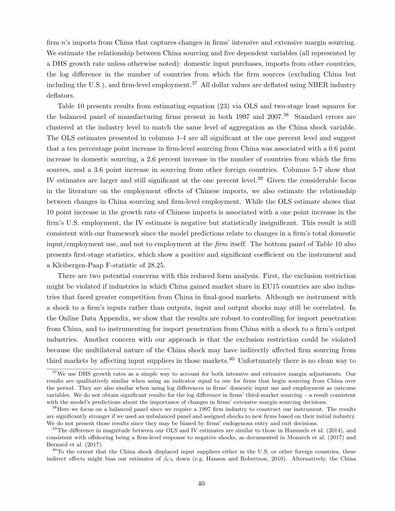
firm n’s imports from China that captures changes in firms’ intensive and extensive margin sourcing.

We estimate the relationship between China sourcing and five dependent variables (all represented by

a DHS growth rate unless otherwise noted): domestic input purchases, imports from other countries,

the log difference in the number of countries from which the firm sources (excluding China but

including the U.S.), and firm-level employment.37 All dollar values are deflated using NBER industry

deflators.

Table 10 presents results from estimating equation (23) via OLS and two-stage least squares for

the balanced panel of manufacturing firms present in both 1997 and 2007.38 Standard errors are

clustered at the industry level to match the same level of aggregation as the China shock variable.

The OLS estimates presented in columns 1-4 are all significant at the one percent level and suggest

that a ten percentage point increase in firm-level sourcing from China was associated with a 0.6 point

increase in domestic sourcing, a 2.6 percent increase in the number of countries from which the firm

sources, and a 3.6 point increase in sourcing from other foreign countries. Columns 5-7 show that

IV estimates are larger and still significant at the one percent level.39 Given the considerable focus

in the literature on the employment effects of Chinese imports, we also estimate the relationship

between changes in China sourcing and firm-level employment. While the OLS estimate shows that

10 point increase in the growth rate of Chinese imports is associated with a one point increase in the

firm’s U.S. employment, the IV estimate is negative but statistically insignificant. This result is still

consistent with our framework since the model predictions relate to changes in a firm’s total domestic

input/employment use, and not to employment at the firm itself. The bottom panel of Table 10 also

presents first-stage statistics, which show a positive and significant coefficient on the instrument and

a Kleibergen-Paap F-statistic of 28.25.

There are two potential concerns with this reduced form analysis. First, the exclusion restriction

might be violated if industries in which China gained market share in EU15 countries are also indus-

tries that faced greater competition from China in final-good markets. Although we instrument with

a shock to a firm’s inputs rather than outputs, input and output shocks may still be correlated. In

the Online Data Appendix, we show that the results are robust to controlling for import penetration

from China, and to instrumenting for import penetration from China with a shock to a firm’s output

industries. Another concern with our approach is that the exclusion restriction could be violated

because the multilateral nature of the China shock may have indirectly affected firm sourcing from

third markets by affecting input suppliers in those markets.40 Unfortunately there is no clean way to

37We use DHS growth rates as a simple way to account for both intensive and extensive margin adjustments. Ourresults are qualitatively similar when using an indicator equal to one for firms that begin sourcing from China overthe period. They are also similar when using log differences in firms’ domestic input use and employment as outcomevariables. We do not obtain significant results for the log difference in firms’ third-market sourcing – a result consistentwith the model’s predictions about the importance of changes in firms’ extensive margin sourcing decisions.

38Here we focus on a balanced panel since we require a 1997 firm industry to construct our instrument. The resultsare significantly stronger if we used an unbalanced panel and assigned shocks to new firms based on their initial industry.We do not present those results since they may be biased by firms’ endogenous entry and exit decisions.

39The difference in magnitude between our OLS and IV estimates are similar to those in Hummels et al. (2014), andconsistent with offshoring being a firm-level response to negative shocks, as documented in Monarch et al. (2017) andBernard et al. (2017).

40To the extent that the China shock displaced input suppliers either in the U.S. or other foreign countries, theseindirect effects might bias our estimates of βCh down (e.g. Hanson and Robertson, 2010). Alternatively, the China

40

Table 10: Estimates of the impact of the China shock on firm-level sourcing

Dependent variable is firm-level change from 1997 to 2007 in:

Domestic No. of Foreign Firm Domestic No. of Foreign Firminputs countries inputs empl. inputs countries inputs empl.

OLS IV

China, DHS 0.064 0.255 0.362 0.097 0.758 0.551 0.670 -0.092(0.010) (0.007) (0.013) (0.007) (0.214) (0.080) (0.198) (0.162)

Constant 0.054 0.144 0.315 -0.075 -0.054 0.098 0.267 -0.046(0.019) (0.013) (0.026) (0.014) (0.039) (0.017) (0.044) (0.032)

N 127,400 127,400 127,400 127,400 127,400 127,400 127,400 127,400

First Stage Statistics Coeff (se) 2.685 (0.505) KP F stat 28.25

Notes: All variables are changes or growth rates from 1997 to 2007. China, DHS is a Davis-Haltiwanger-Schuh growth ratein firm imports from China. Domestic inputs, foreign inputs, and firm employment are a DHS growth rate. No. of coun-tries is the log difference in the number of countries (excluding China, but including the U.S.) from which the firm sourcesinputs. Foreign inputs exclude China. Standard errors are in parentheses and clustered by 439 NAICS industries. In the IVspecifications, firm-level sourcing from China is instrumented by the change in Chinese market share in EU15 countries of aweighted average of the firm’s inputs. KP F-stat is the Kleibergen Paap F-statistic. N is rounded for disclosure avoidance.

control for shocks to a firm’s suppliers in these data, but this could be a fruitful avenue to explore

with richer information on supply-side firm-level networks.

The results in Tables 9 and 10 provide strong support for the empirical relevance of our theoretical

mechanism. First, they show that firms sourcing from China increase their domestic and third market

sourcing substantially more than firms that do not import from China. This is inconsistent with the

predicted responses in a world with independent entry decisions since, as shown in Panel D of Table 7,

under this scenario all firms decrease their domestic sourcing by the same amount. Second, they show

that increased domestic and foreign sourcing occurs not just across, but also within firms. Third, they

rule out firm-specific demand or productivity shocks as drivers of these changes. Most importantly,

the results show that increased firm-level imports from China do not decrease domestic and third

market sourcing –as might be expected in a world with no interdependencies in sourcing decisions–

but instead are associated with increased firm-level sourcing from other markets.

7 Conclusion

This paper provides a new framework in which to analyze the global sourcing decisions of firms in a

multi-country world where production combines multiple inputs. Our model nests the two canonical

models of the extensive margin of exporting, the Eaton and Kortum (2002) Ricardian competitive

model and the Melitz (2003) monopolistic competition with heterogeneous firms. These special cases

highlight the fact that in a general setting, sourcing decisions interact through the cost function, so

that determining the extensive margin of importing must involve solving a 2J -dimensional discrete

choice problem (where J is the number of countries), rather than solving J binary problems as in

canonical models of exporting.

A key contribution of this paper is to overcome these challenges by showing that –under a simple

shock may have led to wage decreases or productivity increases among suppliers that in turn led U.S. firms to increasesourcing from them. To the extent that these changes disproportionately affect industries in which a firm’s inputs wereshocked (e.g., Torres-Ruiz and Utar, 2013), our estimates might be biased up.

41

parametric restriction that is consistent with the data– a firm’s decision to source from one coun-

try is complementary to its decision to source from other countries. These complementarities in a

firm’s extensive margin sourcing decisions underpin our new methodological approach to reduce the

dimensionality of the firm’s problem and solve it. By extending the pioneering work of Jia (2008) to

a multi-firm environment, we recover the key parameters of our model from confidential U.S. firm-

level data on the sourcing decisions of U.S. firms in 67 countries. Armed with these estimates, we

explore the quantitative bite of the key novel features of our framework by studying how a shock to

the potential benefits of sourcing from a country (namely, China) differentially affects the sourcing

decisions of U.S. firms depending on their core productivity and their pre-shock sourcing strategies.

A distinctive characteristic of our framework is that a sectoral import competition shock that does

not simultaneously increase export opportunities may still lead to intraindustry reallocation effects

by which firms sourcing from the shocked country may expand, while firms not sourcing from that

country shrink. We show that a ‘China shock’ calibrated to match the growth in U.S. foreign sourcing

from China between 1997 and 2007 generates qualitative effects consistent with the observed evolution

of U.S. firms’ domestic and third-market sourcing.

Our theoretical framework is necessarily stylized, but it can flexibly accommodate various exten-

sions. As shown in the Online Appendix and further explored in Bernard et al. (2016), it can easily

be extended to include the joint determination of the extensive margin of importing and exporting.

It is also straightforward to incorporate fixed costs of sourcing costs at the input level (see the Online

Appendix) and also at the supplier level. This latter approach is explored by Bernard et al. (2015)

and Furusawa et al. (2016) in their studies of buyer-seller relationships in Japan. Similarly, we have

abstracted from the type of contractual frictions inherent in global sourcing transactions, but as out-

lined in Antras (2016), these contractual aspects can also be incorporated in our framework, thus

permitting a multi-country analysis of the choice between intrafirm versus arm’s-length global sourc-

ing, along the lines of Antras and Helpman (2004). Finally, we believe that the methodological tools

we have developed in this paper, and particularly our application of Jia’s (2008) iterative algorithm

for solving single-agent entry decisions with interdependencies across markets, could be fruitfully

adopted in alternative environments, such as in exporting models with non-constant marginal costs

or in the presence of demand linkages across markets.

42

References

Acemoglu, Daron, Pol Antras, and Elhanan Helpman, “Contracts and Technology Adoption,” AmericanEconomic Review, 2007, 97 (3), 916–943.

Amiti, Mary and Jozef Konings, “Trade Liberalization, Intermediate Inputs, and Productivity: Evidencefrom Indonesia,” American Economic Review, December 2007, 97 (5), 1611–1638.

Antras, Pol, Global Production: Firms, Contracts and Trade Structure 2016. Princeton University Press.

and Elhanan Helpman, “Global Sourcing,” Journal of Political Economy, 2004, 112 (3), 552–580.

and , “Contractual Frictions and Global Sourcing,” in “The Organization of Firms in a Global Economy,”Cambridge, MA: Harvard University Press, 2008.

Arkolakis, Costas, Arnaud Costinot, and Andres Rodrıguez-Clare, “New Trade Models, Same OldGains?,” American Economic Review, February 2012, 102 (1), 94–130.

, Svetlana Demidova, Peter J Klenow, and Andres Rodrıguez-Clare, “Endogenous Variety and theGains from Trade,” American Economic Review, April 2008, 98 (2), 444–450.

Autor, David, David Dorn, Gordon H. Hanson, and Jae Song, “Trade Adjustment: Worker-levelEvidence,” The Quarterly Journal of Economics, 2014, 129, 199–1860.

Autor, David H., David Dorn, and Gordon H. Hanson, “The China Syndrome: Local Labor MarketEffects of Import Competition in the United States,” American Economic Review, 2013, 103 (6), 2121–68.

Bache, Peter and Anders Laugesen, “Monotone Comparative Statics for the Industry Composition,”Working Paper, Aarhus University, 2013.

Barro, Robert and Jong Wha Lee, “A New Data Set of Educational Attainment in the World, 1950-2010,”2010. NBER Working Paper No. 15902.

Bernard, Andrew B. and Teresa C. Fort, “Factoryless Goods Producing Firms,” American EconomicReview Papers and Proceedings, May 2015, 105 (5), 518–523.

, Andreas Moxnes, and Yukiko U. Saito, “Production Networks, Geography and Firm Performance,”Working Paper 21082, National Bureau of Economic Research April 2015.

Bernard, Andrew B, J. Bradford Jensen, Stephen J Redding, and Peter K Schott, “Firms inInternational Trade,” Journal of Economic Perspectives, August 2007, 21 (3), 105–130.

, , , and , “The Margins of US Trade,” American Economic Review, April 2009, 99 (2), 487–493.

, , , and , “Global Firms,” paper commissioned by the Journal of Economic Literature, 2016.

Bernard, Andrew B., Teresa C. Fort, Valerie Smeets, and Frederic Warzynski, “Offshoring andReorganization,” Technical Report, Tuck School of Business 2017.

Bils, Mark and Peter J. Klenow, “Does Schooling Cause Growth?,” American Economic Review, 2000,90, 1160–1183.

Blaum, Joaquin, Claire Lelarge, and Michael Peters, “Non-Homothetic Import Demand: Firm Produc-tivity and Quality Bias,” Unpublished paper, 2013.

, Claire LeLarge, and Michael Peters, “The Gains from Input Trade in Firm-Based Models of Import-ing,” Working Paper 21504, NBER August 2015.

Broda, Christian and David E. Weinstein, “Globalization and the Gains From Variety,” The QuarterlyJournal of Economics, May 2006, 121 (2), 541–585.

Chaney, Thomas, “Distorted Gravity: The Intensive and Extensive Margins of International Trade,” Amer-ican Economic Review, August 2008, 98 (4), 1707–1721.

43

Costinot, Arnaud, “An Elementary Theory of Comparative Advantage,” Econometrica, 2009, 77 (4),1165–1192.

De Loecker, Jan, Pinelopi K. Goldberg, Amit K. Khandelwal, and Nina Pavcnik, “Prices, Markups,and Trade Reform,” Econometrica, March 2016, 84 (2), 445–510.

Eaton, Jonathan and Samuel Kortum, “Technology, Geography, and Trade,” Econometrica, 2002, 70 (5),1741–1779.

, , and Francis Kramarz, “An Anatomy of International Trade: Evidence From French Firms,” Econo-metrica, 2011, 79 (5), 1453–1498.

Feenstra, Robert C. and J. Bradford Jensen, “Evaluating Estimates of Materials Offshoring from U.S.Manufacturing,” Economic Letters, 2012, 117, 170–173.

and John Romalis, “International Prices and Endogenous Quality,” The Quarterly Journal of Economics,May 2014, 129 (2), 477–527.

Fort, Teresa C., “Technology and Production Fragmentation: Domestic versus Foreign Sourcing,” Review ofEconomic Studies, forthcoming.

and Shawn Klimek, “The Effects of Industry Classification Changes on US Employment Compostion,”Technical Report, Tuck School of Business 2016.

Furusawa, Taiji, Tomohiko Inui, Keiko Ito, and Heiwai Tang, “Global Sourcing and Domestic Produc-tion Networks,” Technical Report, mimeo, John Hopkins University 2016.

Garetto, Stefania, “Input Sourcing and Multinational Production,” American Economic Journal: Macroe-conomics, April 2013, 5 (2), 118–151.

Goldberg, Pinelopi Koujianou, Amit Kumar Khandelwal, Nina Pavcnik, and Petia Topalova,“Imported Intermediate Inputs and Domestic Product Growth: Evidence from India,” The Quarterly Journalof Economics, November 2010, 125 (4), 1727–1767.

Gopinath, Gita and Brent Neiman, “Trade Adjustment and Productivity in Large Crises,” AmericanEconomic Review, March 2014, 104 (3), 793–831.

Grossman, Gene M. and Esteban Rossi-Hansberg, “Trading Tasks: A Simple Theory of Offshoring,”American Economic Review, 2008, 98 (5), 1978–97.

Grossman, Gene M and Giovanni Maggi, “Diversity and Trade,” American Economic Review, December2000, 90 (5), 1255–1275.

Grossman, Gene M., Elhanan Helpman, and Adam Szeidl, “Optimal integration strategies for themultinational firm,” Journal of International Economics, 2006, 70 (1), 216–238.

Hall, Robert E. and Charles I. Jones, “Why do some countries produce so much more output per workerthan others?,” Quarterly Journal of Economics, 1999, 114, 83–116.

Halpern, Laszlo, Miklos Koren, and Adam Szeidl, “Imported Inputs and Productivity,” AmericanEconomic Review, December 2015, 105 (12), 3660–3703.

Hanson, Gordon H. and Raymond Robertson, “China and the Manufacturing Exports of Other De-veloping Countries,” in Robert Feenstra and Shang Jin Wei, eds., China’s Growing Role in World Trade,University of Chicago Press and the NBER, 2010, pp. 137–159.

, Raymond J. Mataloni, and Matthew J. Slaughter, “Vertical Production Networks in MultinationalFirms,” Review of Economics and Statistics, 2005, 87 (4), 664–678.

Helpman, Elhanan, Marc Melitz, and Yona Rubinstein, “Estimating Trade Flows: Trading Partnersand Trading Volumes,” The Quarterly Journal of Economics, May 2008, 123 (2), 441–487.

44

Heston, Alan, Robert Summers, and Bettina Aten, “Penn World Table Version 7.0,” 2011. Center forInternational Comparisons of Production, Income and Prices at the University of Pennsylvania.

Hummels, David, Jun Ishii, and Kei-Mu Yi, “The Nature and Growth of Vertical Specialization in WorldTrade,” Journal of International Economics, 2001, 54, 75–96.

, Rasmus Jorgensen, Jakob Munch, and Chong Xiang, “The Wage Effects of Offshoring: Evidencefrom Danish Matched Worker-Firm Data,” American Economic Review, 2014, 104, 1597–1629.

Jia, Panle, “What Happens When Wal-Mart Comes to Town: An Empirical Analysis of the Discount RetailingIndustry,” Econometrica, November 2008, 76 (6), 1263–1316.

Johnson, Robert C. and Guillermo Noguera, “A Portrait of Trade in Value Added over Four Decades,”Review of Economics and Statistics, 2016, forthcoming.

Melitz, Marc J., “The Impact of Trade on Intra-Industry Reallocations and Aggregate Industry Productiv-ity,” Econometrica, 2003, 71 (6), 1695–1725.

and Stephen J. Redding, “New Trade Models, New Welfare Implications,” American Economic Review,March 2015, 105 (3), 1105–1146.

Milgrom, Paul and John Roberts, “The Economics of Modern Manufacturing: Technology, Strategy, andOrganization,” The American Economic Review, June 1990, 80 (3), 511–528.

Monarch, Ryan, Jooyoun Park, and Jagadeesh Sivadasan, “Domestic Gains from Offshoring? Evidencefrom TAA-linked U.S. Microdata,” Journal of International Economics, 2017, 105, 150–173.

Morales, Eduardo, Gloria Sheu, and Andres Zahler, “Gravity and Extended Gravity: Using MomentInequalities to Estimate a Model of Export Entry,” Working Paper 19916, National Bureau of EconomicResearch February 2014.

Olley, G Steven and Ariel Pakes, “The Dynamics of Productivity in the Telecommunications EquipmentIndustry,” Econometrica, 1996, 64 (6), 1263–97.

Oostendorp, Remco H., “The Standardized ILO October Inquiry 1983-2003,” mimeo, Amsterdam Institutefor International Development 2005.

Pierce, Justin R. and Peter K. Schott, “A Concordance between Ten-Digit U.S. Harmonized SystemCodes and SIC/NAICS Product Classes and Industries,” Journal of Economic and Social Measurement,2012, 37, 61–96.

and , “The Surprisingly Swift Decline of U.S. Manufacturing Employment,” American Economic Review,2016, 106 (7), 1632–1662.

Rodrıguez-Clare, Andres, “Offshoring in a Ricardian World,” American Economic Journal: Macroeco-nomics, April 2010, 2 (2), 227–258.

Tintelnot, Felix, “Global Production with Export Platforms,” Quarterly Journal of Economics, forthcoming.

Torres-Ruiz, Luis and Hale Utar, “International Competition and Industrial Evolution: Evidence fromthe Impact of Chinese Competition on Mexican Maquiladoras,” Journal of Development Economics, 2013,105, 267–287.

Vives, Xavier, “Nash equilibrium with strategic complementarities,” Journal of Mathematical Economics,1990, 19 (3), 305–321.

Yeaple, Stephen Ross, “The complex integration strategies of multinationals and cross country dependenciesin the structure of foreign direct investment,” Journal of International Economics, 2003, 60 (2), 293–314.

45

A Estimation Appendix

A.1 Measuring Firm-Level Offshoring Shares

We measure a firm’s total inputs using production worker wages from the Census of Manufactures (CM), totalcost of materials from the Economic Censuses of manufacturing, construction, and mining, and merchandisepurchases from the Census of Wholesale. Inputs from any foreign country j are simply the firm’s total importsfrom j. Domestic inputs are the difference between total inputs and imports. A firm’s share of inputs fromcountry j, χij , is computed as imports from j divided by total input purchases. Additional details are indescribed in the Online Data Appendix.

A.2 Estimation of the Trade Elasticity

Table A.1 presents the first stage regressions for the IV estimates of θ, where we instrument for country wagesusing population. As expected, the estimated coefficient on population is negative and significant at the fivepercent level. The F-statistics for the excluded instrument is 6.49. In unreported results (available in ouronline replication files), we verify that the Anderson-Rubin F test and χ2 test of significance of the endogenousregressors are statistically significant at the five percent level.

Table A.1: First stage regressions for trade elasticity estimates

Dependent variable is log HC adj. wage

log population -0.32(0.12)

log distance -0.20(0.14)

log R&D 0.32(0.09)

log KL 0.14(0.17)

Common language -0.05(0.17)

Control of corruption 0.22(0.12)

log no. of firms -0.04(0.07)

Constant -1.48(0.81)

R2 .883Observations 57

Notes: First stage regressions for the IV estimatespresented in Table 4. Wage is the log of the humancapital-adjusted wage. Population is the excludedinstrument.

A.3 Estimation Results and Counterfactual Predictions

In this Appendix, we provide three additional tables related to our structural estimation and counterfactuals.Table A.2 compares the share of imports and importers in the data (as in Table 1), in the baseline model, and inthe model with common fixed costs across countries. Table A.3 reports our estimation and counterfactual resultsfor various alternative parameter values. Table A.4 contains details on the performance of our application ofJia’s (2008) algorithm.

A.4 China Shock Measure for Reduced Form Estimates

We instrument for changes in firm-level sourcing from China using changes in a novel measure of Chinesecomparative advantage in a firm’s inputs. Specifically, we measure Chinese comparative advantage in the

46

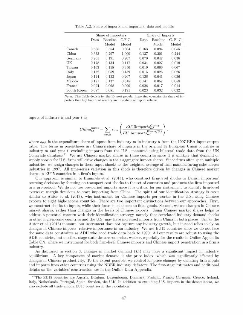
Table A.2: Share of imports and importers: data and models

Share of Importers Share of ImportsData Baseline C.F.C. Data Baseline C. F. C.

Model Model Model Model

Canada 0.585 0.554 0.304 0.163 0.094 0.055China 0.333 0.297 1.000 0.137 0.201 0.244Germany 0.201 0.191 0.207 0.070 0.047 0.036UK 0.178 0.134 0.117 0.034 0.027 0.019Taiwan 0.163 0.158 0.356 0.019 0.066 0.067Italy 0.132 0.059 0.159 0.015 0.025 0.026Japan 0.124 0.133 0.207 0.126 0.041 0.036Mexico 0.121 0.137 0.315 0.141 0.057 0.058France 0.094 0.068 0.090 0.026 0.017 0.014South Korea 0.087 0.081 0.191 0.023 0.032 0.032

Notes: This Table depicts for the 10 most popular importing countries the share of im-porters that buy from that country and the share of import volume.

inputs of industry h and year t as

Chinainputht =∑m∈h

smh

(EU15importsChinamt

EU15importsWorld/USmt

),

where smh is the expenditure share of inputs from industry m in industry h from the 1997 BEA input-outputtable. The terms in parentheses are China’s share of imports in the original 15 European Union countries inindustry m and year t, excluding imports from the U.S., measured using bilateral trade data from the UNComtrade database.41 We use Chinese market shares in these countries since it is unlikely that demand orsupply shocks for U.S. firms will drive changes in their aggregate import shares. Since firms often span multipleindustries, we assign changes in these input shocks as the weighted average of firm manufacturing sales acrossindustries in 1997. All time-series variation in this shock is therefore driven by changes in Chinese marketshares in EU15 countries in a firm’s inputs.

Our approach is similar to Hummels et al. (2014), who construct firm-level shocks to Danish importers’sourcing decisions by focusing on transport cost shocks to the set of countries and products the firm importedin a pre-period. We do not use pre-period imports since it is critical for our instrument to identify firm-levelextensive margin decisions to start importing from China. The spirit of our identification strategy is mostsimilar to Autor et al. (2013), who instrument for Chinese imports per worker in the U.S. using Chineseexports to eight high-income countries. There are two important distinctions between our approaches. First,we construct shocks to inputs, while their focus is on shocks to final goods. Second, we use changes in Chinesemarket shares, rather than changes in the levels of Chinese exports. Using Chinese market shares helps toaddress a potential concern with their identification strategy–namely that correlated industry demand shocksin other high-income countries and the U.S. may have increased imports from China in both places. Unlike theAutor et al. (2013) measure, our instrument does not capture any industry growth, but instead relies solely onchanges in Chinese imports’ relative importance in an industry. We use EU15 countries since we do not facethe same data constraints as ADH who need trade data back to 1990. All our results are robust to using theADH countries, but our first stage statistics are somewhat weaker, especially for the results in Online AppendixTable C.9, where we instrument for both firm-level Chinese imports and Chinese import penetration in a firm’sindustry.

As discussed in section 3, changes in market demand (Bi) may have a significant impact in industryequilibrium. A key component of market demand is the price index, which was significantly affected bychanges in Chinese productivity. To the extent possible, we control for price changes by deflating firm inputsand imports from other countries using the NBER industry deflators. The first-stage estimates and additionaldetails on the variables’ construction are in the Online Data Appendix.

41The EU15 countries are Austria, Belgium, Luxembourg, Denmark, Finland, France, Germany, Greece, Ireland,Italy, Netherlands, Portugal, Spain, Sweden, the U.K. In addition to excluding U.S. imports in the denominator, wealso exclude all trade among EU15 countries in the calculation.

47

Table A.3: Sensitivity of parameter estimates and counterfactual predictions to alternative values forθ, κ, and σ

Variation in θ Variation in κVariation

in σBaseline θ = 1.3 θ = 2 θ = 2.85 κ = 3 κ = 4 κ = 5 σ = 2.79 σ = 5

Parameter estimatesB 0.122 0.121 0.123 0.124 0.103 0.118 0.132 0.237 0.072

βfc 0.023 0.030 0.020 0.014 0.040 0.024 0.020 0.017 0.039

βfd 0.192 0.209 0.188 0.187 0.414 0.224 0.118 0.002 0.421

βfl 0.871 0.939 0.868 0.872 0.778 0.856 0.901 0.944 0.768

βfC -0.394 -0.434 -0.395 -0.394 -0.393 -0.389 -0.415 -0.468 -0.393

βfdisp 0.939 0.935 0.932 0.927 1.312 0.989 0.819 0.633 1.318

Median fixed cost range across countriesMinimum (in tsd USD) 10 14 9 7 19 11 9 5 19Maximum (in tsd USD) 56 82 50 35 175 65 42 29 175

Counterfactual predictionsPrice index change (in percent) -0.189 -0.268 -0.167 -0.113 -0.430 -0.215 -0.134 -0.072 -0.408Change in third country sourcing by 1.5 3.6 0.9 -0.6 0.1 1.3 2.0 -0.3 1.5new importers from China (in percent)

Gross increase in U.S. sourcing 0.113 0.345 0.053 0.000 0.011 0.090 0.141 0.000 0.096(in percent of total U.S. sourcing)

Net change in U.S. sourcing -0.527 -0.554 -0.519 -0.497 -0.854 -0.571 -0.433 -0.307 -0.885(in percent of total U.S. sourcing)

Notes: This table presents Step 3 estimation results and counterfactual predictions for alternative parameter values for the firm-level trade elasticity θ,the shape parameter of the Pareto distribution κ, and the elasticity of substitution σ.

Table A.4: Cardinality of differences in bounds

Cardinality of differences 0 1 2 3 4 5 6 7 8 9 10 - 25 ≥ 26in bounds

Baseline 11220190126 0 918094 84695 6693 376 16 0 0 0 0 0Variation in θ θ = 1.3 12359440019 0 3682595 600585 98164 15680 2474 444 26 12 1 0

θ = 2 12073844987 0 515622 36813 2342 233 3 0 0 0 0 0θ = 2.85 12897360000 0 0 0 0 0 0 0 0 0 0 0

Variation in κ κ = 3 12343521037 0 801134 72030 5290 477 25 5 2 0 0 0κ = 4 12786062392 0 1034458 94304 7843 902 99 2 0 0 0 0κ = 5 11792382315 0 1107735 101502 7671 719 49 9 0 0 0 0

Variation in σ σ = 2.79 13145760000 0 0 0 0 0 0 0 0 0 0 0σ = 5 12304230446 0 2885568 476715 72738 12206 1947 353 27 0 0 0

Notes: This table displays the number of firm (productivity and fixed cost draws) and parameter combinations for which the cardinality of thedifferences in the bounds reached a particular value. While the productivity and fixed cost draws are held fixed during the estimation process,the parameter vector, δ, varies through the iterations of the estimation process. We allow the differences of the bounds to be less than 26, beforewe would revert to evaluating the objective value of the firm’s problem at the bounds and a small number of random values for the countries inthe bound. Since this cardinality of the differences in the bounds is never very high, we always solve accurately the problem of the firm.

48