THE MAIN DETERMINANTS OF INSURANCE PURCHASE AN EMPIRICAL STUDY ON CROP INSURANCE POLICIES IN

FRANCE

Enjolras G., Sentis P.

Paper prepared for presentation at the 12th EAAE Congress ‘People, Food and Environments: Global Trends and European Strategies’,

Gent (Belgium), 26-29 August 2008

Copyright 2008 by [Enjolras G., Sentis P.] . All rights reserved. Readers may make verbatim copies of this document for non-commercial purposes by any means, provided that this copyright notice appears on all such copies.

THE MAIN DETERMINANTS OF INSURANCE PURCHASE AN EMPIRICAL STUDY ON CROP INSURANCE POLICIES IN FRANCE

Enjolras G.1,2,3*, Sentis P.1,2,4

1 University of Montpellier I - Faculté d'Administration et Gestion de Montpellier, Avenue de la Mer, 34054 Montpellier Cedex 1, France.

2 CR2M, Montpellier, France 3 INRA - LAMETA, 2 place Pierre Viala, 34060 Montpellier Cedex 1, France.

4 GSCM Montpellier Business School * Corresponding author: enjolras@supagro.inra.fr

Abstract- Using data for 2002-2005 on a representative survey of French farms (FADN-RICA), we investigate the different factors that lead farmers to insure against crop risk. Our analysis takes into account a mix of both standard individual, financial and agricultural criteria. Cross-sectional and longitudinal analyses as well as logistic regressions underline the main differences between insured and non-insured farms. Compared to non-insured farms, we find that insured farms present greater financial and agricultural sizes, a more diversified production and have been motivated by the occurrence of recent catastrophic climatic events. Although essential in the cross-sectional analysis, the influence of financial parameters in the decision to insure is mitigated. On the other hand, the agricultural characteristics of the farms confirm their leading influence for the subscription of crop insurance policies.

Keywords- Insurance, Demand, Crop insurance, Catastrophe risk

1

1 Introduction

In recent years, the market for catastrophic risk has considerably grown and the insurance, reinsurance and financial markets contribute now to hedge more natural hazards than ever (Froot, 2001). Structural reforms of the States' subsidizations have been particularly important in the agricultural sector and their aim is always the same: the introduction and the development of private insurance and the encouragement for a multirisk coverage. If we consider the catastrophic insurance problem from the farm’s point of view, we notice that the most studied criterion is their solvency. In this domain, literature mainly refers to insurance companies (Zanjani, 2002, Kelly and Kleffner, 2003). This leads to the question of their efficiency to propose products adapted to insurance demand. In facts, natural hazards mainly concern human beings and the agricultural sector. As a sign of their vulnerability, they both benefit from a State’s intervention in most developed countries when a catastrophe occurs. This implication of the public authorities has become necessary due to market imperfections in catastrophe risk sharing (Niehaus, 2002). Moreover, it encourages the development of policies, which will fit the new needs for coverage. With human beings, the major preoccupation comes from the material’s exposure and housing in particular. According to recent surveys with large French insurance companies, this stake is by far the most important in financial terms. It also uniformly concerns all types of activities, including agriculture. We notice that literature is abundant on this subject and considers the problems from the points of view of the insurers (Choi and Weiss, 2005), the insured (Grace et al., 2004) or the market (Lustig and Van Nieuwerburgh, 2005). Conversely, literature is quite scarce about the financial aspects of specific agricultural insurance mainly for the so-called crop insurance. We can refer to the market studies realized by Wang and Zang (2003). Harrington and Niehaus (1999), also cited by Puelz (1999), insist on the specificities of each business, which determines the needs for tailor-made insurance. If we follow their reasoning, agricultural risk management should be treated in the same way than agricultural financial management. As presented by Harrington and Niehaus (1999), this supposes to introduce a wide range of financial parameters relative to the size of the business, its cash ratio, its financial distress and the activities’ structure. Then we can use these financial criteria in addition to traditional agricultural ones in order to establish the decision rules that lead farmers to insure. The paper is mainly centered on this question. Literature devoted to crop insurance is not specifically oriented towards financial issues. Among the explicative variables for crop insurance subscription, we find the farm size, the debt-to-asset ratio (also known as the financial leverage) and the age and education of the farmer. However, these recurrent indicators often restrict the field of potential dependant variables. For example, no study proposes to detail meteorological variables whereas the final yield essentially depends on the climate. Among the potential variables, precipitations are the most frequently cited (Van Asseldonk et al., 2002, Blank et al., 1996). Similarly, the financial variables other than the debts are left aside. In some studies, the turnover or the farmer’s income is included in the analysis (Mishra et al., 2003, Van Asseldonk et al., 2002, Blank et al., 1996), as well as the subsidization level (Glauber, 2004, Mishra et al., 2003). Otherwise, the different risk management options are taken into account, for instance the use of chemical products (Serra et al., 2003), irrigation or activities diversification (Serra et al., 2003, Blank et al., 1996, Goodwin, 1993). We try to be as

2

exhaustive as possible by integrating in our analysis a set of diversified variables relative to all characteristics of the farms: individual, financial and meteorological parameters. From a geographical point of view, previous researches mainly refer to the United States case (for instance, Knight and Coble, 1997). This country has developed overtime (in 1980, 1994 and 2000) a stronger crop insurance system (Glauber, 2004). Nevertheless, some countries of the southern European Union have also successfully developed integrated insurance programs (Garrido and Zilberman, 2007). Nowadays, in these most advanced systems, insurance policies subscription reaches about 50% to 60% of eligible farms. The French case is particularly interesting because crop insurance has considerably been expanding since the 2004 reform. In the past, only hail and storms were really covered because their characteristics made them insurable without any subsidies. All the other hazards were covered using a national guarantee fund. Since 2004, an experimental test of multi-peril crop insurance is operated at the national level. It involves both the State and historically focused on agriculture private insurers. Although such a reform completely changed the coverage of natural events in French agriculture, it has received a very superficial treatment and literature is quite scant on this subject. We also consider the problem on a national scale in order to get a representative overview of the situation. This approach is facilitated by the data of the Farm Accountancy Data Network (FADN-RICA). Moreover, global criteria are accepted by all types of studies, recent or not (Sherrick et al. 2004, Serra et al., 2003, Goodwin, 1993). Then, the experimental scheme of this paper allows examining three major concerns: Are financial, individual and catastrophic characteristics of farms subscribing crop insurance policies determinants to insurance decision? Does the subscription of such policies improve the financial wealth and the performances of the firms? Are results consistent along the observation period overlapping the implementation of multi-peril crop insurance in France? The outline of the paper is organized as follows. In a first section, we analyze the agricultural insurance system in France whose current evolution is captured by our data. In a second section, we consider the theoretical and empirical settings of the study. Sections three to five examine the three main questions addressed by the paper according to our methodology: first, the cross-sectional analysis allows discriminating between the insured farms and non-insured firms. Second the longitudinal tests show the change in the different variables between both sub-groups. Finally, the logistic regressions accurately examine the importance of financial variables in the insurance decision. The paper’s most salient conclusions are summarized in section six.

2 The agricultural insurance system in France The French insurance system in agriculture has been developed more than forty years ago under the supervision of the State. Until 1964, there did not exist any integrated coverage system in France. After a series of droughts, a public indemnity mechanism called the National Guarantee Fund for farming calamities (FNGCA) is created. It is equitably financed by the Government Budget and by taxes on compulsory standard insurance policies subscribed by farmers. It covers farming calamities defined as “non insurable damages of exceptional importance due to abnormally intense variations of a natural hazard”. During its existence, losses of crops due to frost or drought indemnified by the FNGCA have accounted for some 75% of total indemnities accorded by the Fund.

3

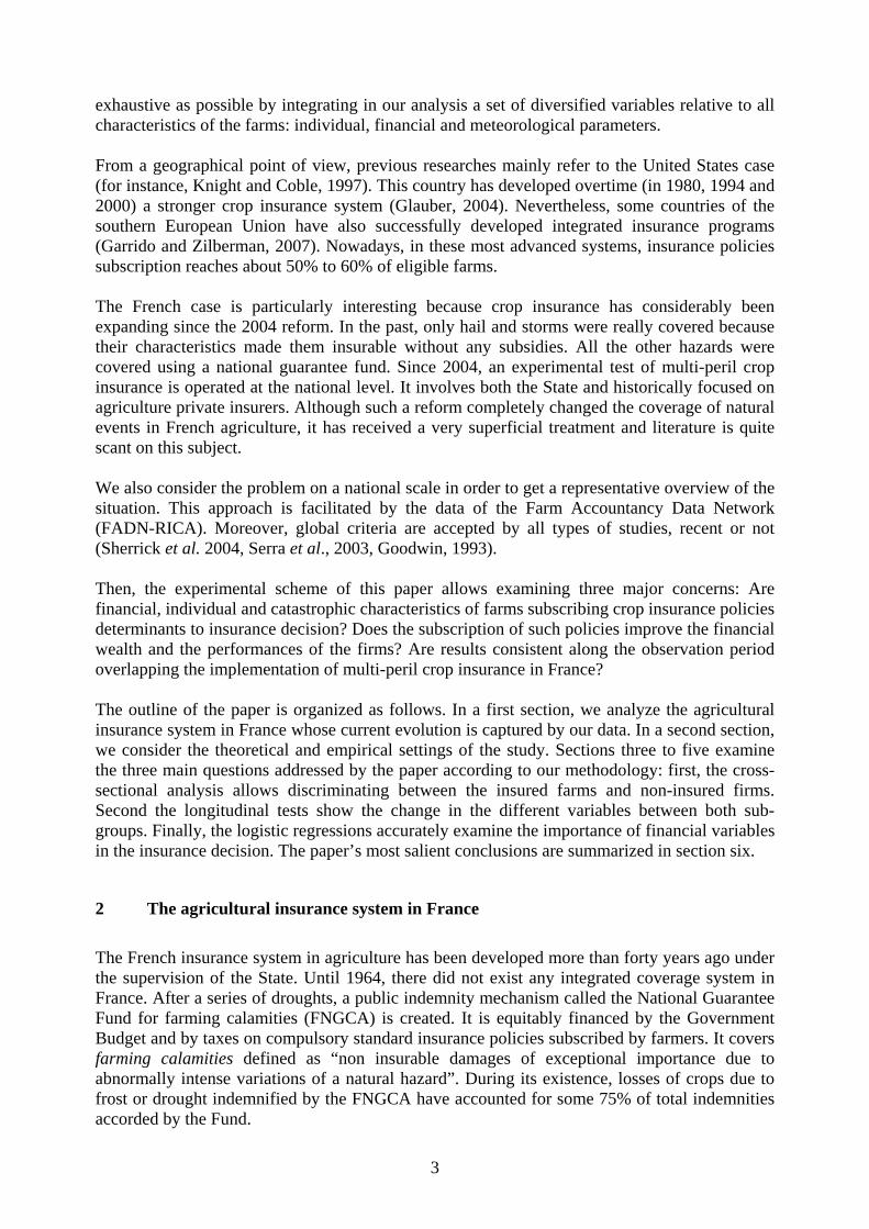
Among insurable risks, hail is historically the main covered risk and it has been partially subsidized for arboriculture, the most exposed activity. The occurrence of numerous hail episodes in the arboricultural regions between 1990 and 1995 has pushed insurers to raise the premia and the deductibles in the fruit and vegetable sector. These increases have helped producing a vicious circle of adverse selection and of tariff increases. Consequently, insured farmers were the less affected by hail. This situation was inducing a financial transfer from lesser risk farming operations (large crops), to those carrying a more significant risk (arboriculture). Facing these constraints, an opportunity for the development of global insurance has been given at the end of the 1990s. First, an agricultural agreement of the World Trade Organization allowed classifying public sector aid to insurance (“Green box”) under certain conditions. Second, the development of aid to insurance in North America (US, Canada) and Southern Europe (Spain, Italy, Greece) provided some experiences. Third, there was a global trend towards the liberalization of agricultural policy, which was likely to increase agricultural prices volatility and therefore the exposure of farmers to natural hazards. In order to develop private insurance, the French Ministry of Agriculture and Fisheries decided to continue subsidizing traditional hail insurance and the FNGCA. Moreover, it extended its subsidies to combined guaranties and weather multirisk insurance in the 2002 Finance Law. New policies should combine hail and frost guarantees for fruits and vineyards and propose weather multirisk insurance for crops on the stalk. The following Table 1 details the insured risks and their scope in 2005 for each kind of crops.

Insurable crops Insured risks Scope Corn and large assimilated crops other than found below

Hail Weather multirisk

55% of national surface 25% of the surface

Vineyards Hail Weather multirisk

60% of national surface 0.5% of national surface

Fruits and garden vegetables Hail Weather multirisk

62% of national surface 1.2% of national surface

Tobacco Weather multirisk 100% of national surface Source: French Ministry of Agriculture.

Table 1 – Main crops, proposed policies and their scope For year 2005, about 20% of farmers have subscribed 57,900 multirisk contracts. This represents an amount of 3,4 million insured hectares, €3 billion insured capital and €82 million premia, whose €50 million are subsidized and €17.4 million come from various State helps. Until 2008, this system remains experimental but it will probably be extended after this period1.

1 As a consequence of French elections, the new system modalities are still not defined in March 2008.

4

3 Theoretical and Empirical Settings As we already pointed out in the introduction, the experimental scheme of this paper allows examining major concerns about the main determinants to insurance decision that lead farms to insure against crop risk. To answer these questions, we detail in the followings subsections our variables and the main assumptions of our model.

3.1 The data

The study uses a survey of farmers in France belonging to the Farm Accountancy Data Network (FADN). Data are accounted for each year from a representative sample of farms, whose size can be considered as commercial. We use a set of data selected through three criteria: localization, economic size and farms major productions. Within the original database, we only select farms that have continuously appertained to the sample from 2002 to 2005. We also restrict the analysis to farms that may be concerned with crop insurance. Finally, our sample includes 4,700 farms. In the following subsections, we detail the main explanatory variables that enter in the analysis. We choose to detail a wide range of potential factors including financial and meteorological variables, often missing in the literature.

3.1.1 Insurance

For the purpose of our analysis, we selected a variable indicating the eventual subscription of a private crop insurance policy. This can be found only for the years 2002 to 2005, which delimitates our temporal analysis. For the same period, the database also gives the amount of perceived indemnities. Thus, our study covers the time of crop insurance regime reform in France. Its effects are marginal during years 2002 and 2003 because the system was only experimented in some places. In 2004 and 2005, nearly all the farmers who subscribed a crop insurance policy against hail were offered the extension to other risks2. Moreover, the range of covered crops is also extending over the years.

3.1.2 Financial and economic indicators

Although neglected in crop insurance literature, the farmers' financial wealth has to be considered as an essential parameter in the decision to insure (Harrington and Niehaus, 1999). The idea is that the largest businesses are more willing to cover their potential losses because their stakes are higher. Moreover, we can infer the indebted farms are also asking for a greater coverage. Thus, the financial leverage should appear as positively correlated with the use of crop insurance.

2 For the leading insurer, which trusts 90% of this new market, guaranteed risks are: sunburn, excess of water, excess of humidity, excess of temperature, frost, hail, floods, hard raining, excess of snow, drought, storm and heat whirl.

5

For the purpose of our analysis, we consider the main economical and financial indicators: - Annual turnover, in €uros. - Invested capital, in €uros. - Financial leverage = Net financial debts / Shareholder’s equity. - Cash disposals = Cash and equivalents / Current asset. - Cash ratio = (Cash + Marketable securities) / Current liabilities. - Return on equity (ROE) = Net income / Shareholders' equity. - Return on capital employed (ROCE) = Operating income / Invested capital. - Revenue per are, in €uros per are. Such indicators, which are strong references in finance, should provide a clear and unbiased view of the financial wealth of the agricultural firms.

3.1.3 Individual indicators

In the analysis, we take into account standard individual indicators for the farm manager such as its age, sex and education level. We can also consider whether a single farmer or a group of farmers exploits the farm. One can think that insured farmers are more educated and have a greater experience than non-insured one. Otherwise, young farmers may be more sensitive to new risk management products as they can receive more subsidies for their insurance policies.

3.1.4 Agricultural indicators

Among the agricultural area indicators, we consider the total, cultivated and irrigated surfaces. We also take into account the farm’s cultures portfolio and its technical economic-activity specialization (vegetables, cattle, or both). In fact, the diversification of the activities is a way to stabilize the annual turnover of the farm. Then, it can be assimilated to a substitute to specific insurance products. Irrigation is also perceived as a mean to hedge crop risk because it reduces soil moisture and desiccation, and increases yield return. On the contrary, biological agriculture seems to be a more risky activity.

3.1.5 Geographic and Weather indicators

The FADN database offers direct ways to determine the location and altitude of the farm and if it is located in a less favored area. Then, we can associate to each place different weather indicators3 that are considered as relevant by literature. We use the annual mean temperature, the annual cumulated precipitations and the annual cumulated hours of sun. Starting from these original variables, we convert them by taking the square deviation from their average4 for each year. Then, we can capture the farmers' sensitivity to excessive variations of the climate. We can assume that farmers are risk-averse against excessive variations and that the most exposed will subscribe crop policies. On the contrary, adverse selection effects may put them out-of-the-market as a consequence of catastrophic results for the insurance company. One can also consider that after a major event like drought or excessive rainfall, the farmers will be more willing to insure their crops. In contrast, the lack of catastrophic events may not be an incentive.

3 Data come from the French National Institute for Agronomic Research weather stations, in partnership with Météo France. We display the indicators for each place taking into account the region and the altimetry. 4 Average is based on the ten years before the decision to insure.

6

3.2 Summary of the main assumptions

Considering the former variables and their potential scope on insurance, we can formulate some assumptions that are tested in the paper: H1: As previously argued, the size and the wealth of farms are proxies for their exposition to crop risk. We expect the largest businesses are more willing to get an insurance coverage. The effect should be captured through standard financial criteria: the annual turnover, invested capital, as well as the financial and economic returns. In agriculture, the correlation should be the same between insurance, the cultivated surface and the "crop portfolio". H2: We also guess that risk-averse farmers should more prone to insure. Criteria for risk aversion can be found in the number of cultivated crop and the irrigated surface. The meteorological variables enter in the frame because abnormal variations of the weather, whether negative or positive, may lead the farmers to insure more. Experienced and more educated farmers would also be more interested in coverage. H3: We finally presume there exists a fidelity effect in crop insurance: farmers who have already subscribed an insurance policy the year before remain insured. The effect should be more pronounced for farmers who have already received indemnities.

4 The characteristics of farms subscribing crop insurance contracts In this section, we look for the fundamental differences between the agricultural firms: the ones that insure themselves and the others.

4.1 Methodology

According to our experimental scheme and to our sample, we can make significant distinctions between the farms depending on whether they are insured or not. At first, we look at some summary statistics. Then, to confirm the results, we use the Mann-Whitney’s nonparametric statistical test.

3.2 Summary statistics

In order to offer a first view of the situation of insured and non-insured farms, we detail hereafter in Table 2 some summary statistics for the years 2002 to 2005. The variables are organized in order to take into account the main characteristics of the farm: agricultural, financial and meteorological. The observed mean and median are reliable indicators due to the significant number of farms (4,700) observed during four years in our sample. The results are quite similar comparing the mean and the median of the two subgroups. This is true for the individual, agricultural and meteorological (excepted for the temperature) variables. We clearly observe that insured farms are bigger than non-insured one (financial and agricultural sizes) and in a better wealth (financial leverage, cash flow). Insured farms are also the most diversified in terms of cultures and they use more irrigation, which is a sign of risk-aversion. Moreover, we can see that weather conditions are more “extreme” for insured farms.

7

Variables Mean Median

Category Detail All Insured Non-insured All Insured Non-

insured Insured (prob.) 0.44 1 0 0 1 0Insurance Indemnity (in €) 663.57 1214.67 228.69 0 0 0Age (in years) 46.44 46.21 46.62 47 46 47Individual

indicators Sex (1=Man) 0.93 0.94 0.93 1 1 1Total area (in ares5) 9388 11052 8075 7645 9270 6655Cultivated area (in ares) 8807 10388 7559 7160 8616 6166Surface Irrigated area (in ares) 601 925 346 0 0 0

Cultures Number of cultures 6.60 7.19 6.14 7 7 6Mean temperature 0.23 0.24 0.22 0.17 0.16 0.18Cumulated precipitations 19803 21424 18525 10692 11273 10501

Meteo indicators (avg. dev.) Cumulated hours of sun 32625 34529 31123 5100 5100 5100

Annual turnover (in €) 213456 221599 207031 167045 177889 158417Invested capital (in €) 444239 467114 426188 367825 386761 352816Financial leverage 0.59 0.55 0.62 0.33 0.33 0.32Cash disposals 0.04 0.04 0.04 0.05 0.05 0.05Cash ratio 0.48 0.46 0.49 0.18 0.18 0.19Return on equity 0.41 0.38 0.43 0.27 0.29 0.26Return on capital employed 0.25 0.24 0.26 0.19 0.19 0.20

Economic and financial indicators

RPA (in € per are) 43.23 17.84 63.26 3.24 4.37 2.31 Legend in rows: in yellow, the highest values for the mean and the median.

Table 2 - Summary statistics for crop insurance use (all years)

One can notice that there remain some differences between the mean and the median, which means that distributions of the different indicators’ values are rather different. This phenomenon mainly concerns the financial indicators (financial leverage, ROE, revenue per are). To confirm these results and provide more interpretations, we consider now a cross-sectional analysis.

4.2 Cross-sectional analysis

Looking at summary statistics underlined some differences in the distribution of some variables between the insured and the non-insured. To compare these two groups, which are not of the same size, we perform for each variable a Mann-Whitney test. In each case, the result is given by the p-value. A small one indicates that the difference between the two groups is significant and consequently that medians are statistically different. The sign of the U-statistic indicates the direction of the relationship. Results are provided in Appendix 1 for each variable and for 2002 to 2005. We can conclude whether the difference is significant or not between the two groups and over the years. Our first control variable indicates that the insured perceive more indemnities than the non-insured, which is a sufficient incentive to get insured. Moreover, it may justify the increasing success of crop insurance in France. Among the financial variables, the turnover and the invested capital are significantly higher for the insured during the four years. It is also true for the ROCE. The financial leverage is also higher for the insured but this effect is only significant in 2005. Conversely, there’s no difference between the groups according to the cash ratio and the ROE. Considering now the

5 1 are = 0.0247 acre

8

agricultural variables, we notice a clear and positive difference between the groups: the insured produce more culture varieties on a higher (irrigated) area. Moreover, the product per surface-unit is clearly higher for the insured. The meteorological variables provide more surprising results. We could suppose that the insured would suffer from a wider range of climatic conditions from one year to another. In fact, this assumption is not verified as the sign of the difference changes over the years. The associated coefficients become simultaneously positive and very significant in 2004. This is not surprising if we consider that 2003 was in France a hard year with scorching heats and a serious deficit of rain. These extreme conditions may have justified a greater need for insurance on the affected areas. It seems that the effect is completely opposite in 2005, as 2004 was quite a normal year. We also notice that the values of the different tests globally increase in 2005, compared to 2004, for each variable. This occurs at the moment when crop insurance is generalized from hail to multi-peril. It probably means that the effects noticed above are reinforced after the introduction of additional coverage. Such an effect has already been observed during the various reforms of the US crop insurance regime (Serra et al., 2003).

5. Situation over the years of farms that subscribed crop insurance policies

In this section, we look for the situation of agricultural businesses that decide to insure for a given year. The idea is to observe whether the situation of the farms significantly changes when they get insured. The comparison is done with farms that do not insure.

5.1 Methodology

Our sample can be exploited during four years, which means we can observe the evolution of the farms with two possible references in 2003 and 2004. Starting from these two points, we can consider an insured farmer on year 0 and look at his situation in year -1 and year +1. Consequently, farmers insured in 0 may not be insured in -1 and/or +1. Then, we compare the evolution of our variables over the years between the insured and the non-insured. For instance, will insured in 0 have significantly higher debts in +1 than non-insured at the same time? The same reasoning applies for all variables.

5.2 Longitudinal analysis

The first step of the analysis is to select a year and to divide the sample according to whether farmers are insured or not. As we still compare two unpaired subpopulations over the years, we perform for each variable a Mann-Whitney test. In each case, the interpretation is given by the value of the test and the p-value. A small one indicates that the difference between the two groups is significant and consequently that medians are statistically different. The sign of the Z-statistic indicates the direction of the relationship. The results of the longitudinal analysis are provided in Appendix 2 for each variable and for each year of reference, 2003 or 2004. Then, we can conclude if the difference is significant or not between the two groups and the scope of time. We notice that financial variables are among the most significant. Let’s consider first the amount of indemnities. We first clearly note that this variable is always significant when the analysis is centered on 2003, while it is never the case when centered on 2004. The comparison

9

of the situation between 2002 and 2003 leads to a significant and positive value: this means that the amount of indemnities during the period increases much for farmer who will insure in 2003 than for those who won’t insure. Between 2003 and 2004, it is the contrary, as indicated by the negative sign. This means that the variation of the indemnities is strangely more favorable to farmers who didn’t insure the year before. Over the period 2002-2004, the balance remains in favor of the insured, which seems normal, considering the insurance’s aim is to provide more wealth for the subscriber. Unfortunately, we cannot perform the same comparison for the years 2003 to 2005, as none of the statistics is significant. Few variables present a uniform sign along the different studied periods. It is the case of the financial leverage. It seems that the debts increase much faster for the insured over the period. It is also the case for the cultivated surface. Then, insured farmers increase their risk by expanding their cultures and their debts. This fact is corroborated by observing the cash variable between 2003 and 2005, whose variation is negatively more important for the insured (at the 10% level). This result is also in phase with literature (Knight and Coble, 1997). We also notice that the revenue per surface-unit increases much more for the insured once the private insurance system is launched (after 2004). Meteorological variables present significant results and we find again the mechanism detailed in the cross-section analysis. Until 2004, the insured bear more excess (negative or positive) temperature, precipitations and sunlight. Between 2004 and 2005, it is the contrary. This fact confirms the increase of the insurance subscriptions in 2004 by farmers who suffered from the 2004 climatic accident. The other variables cannot be correctly interpreted, whether because they are not significant or their sign changes depending on the focus on 2003 or 2004. We can deduce that the effects of insurance are quite ambivalent depending on the study period. After have been insured in 2003, farmers perceive less indemnities but increase their size, turnover and return, compared to the non-insured. For farmers insured in 2004, the benefits procured by insurance are not evident, whilst the financial and agricultural indicators are more favorable to the non-insured.

6. Revisiting the main determinants of crop insurance

Our analysis introduces two major focuses on the financial wealth of the farms and on meteorological parameters, often neglected in crop insurance literature. We shall now test the impact of these parameters on insurance purchasing.

6.1 Methodology

Following previous analyses on the demand of crop insurance (see e.g. Glauber, 2004, or Garrido and Zilberman, 2007), we assume insurance purchase is influenced by a certain number of farm characteristics. The dependant variable is a dummy indicating whether the farmer is insured or not for the given year. We enter in the analysis the entire variables described above. To capture the impact of a previous subscription, we introduce two lagged variables indicating if the farm was insured the year before and the amount of the perceived indemnities6. In order to extend our previous analyses, we also wish to capture the influence of the initial education level of the farmer and the location of the farm. 6 These data are only available for years 2003, 2004 and 2005.

10

For the purpose of our study, we first estimated a series of logistics regressions with the same variables for each year of our sample. Then, we estimate a global model based on data for the years 2003 to 2005

6.2 Regressions year by year

This type of comparison is inspired from Serra et al. (2003) in order to measure changes in demand for crop insurance over the years. We notice that the same variables remain significant over the years: for instance, the fact to have been insured the year before considerably increases the probability to insure the current year. Such a result has already been noticed by the insurers, whose efforts are concentrated on the search for new customers, rather than on the conservation of their customers. The perception of indemnities is also a key criterion: farmers insure if they increase their probability to perceive more indemnities. Financial variables are surprisingly not significant at all compared to agricultural ones: cultivated and irrigated surfaces and the number of different vegetable cultures, which have a positive effect on the decision to insure. Farms that are centered on vegetables are also more willing to insure. The weather is only significant when an extreme event occurred the year before

6.3 Global logistic regression

When merging the samples for years 2003 to 2005, we get a new database with 15,820 observations. Then, we estimate a logistic regression with the same parameters. The results are given in Appendix 3. Among the significant variables, we still find the impact of previous insurance subscription and indemnities. The age has a negative influence on the policy subscription, which is in accordance with the efforts made by the French government to subsidize insurance policies for young farmers. The agricultural variables referring to the cultivated surface and the number of cultures are also significant but their impact is quite modest on the probability of subscription. The technical specialization of the farm has also a significant influence on insurance: farms whose main activity is the production of vegetables are more exposed and then they are more willing to get insured. The financial variables are globally non significant and the global regression does not confirm some results shown with longitudinal and transversal analysis. There is only one significant variable: the revenue per surface-unit, which strangely tends to decrease the probability to insure. In the same way, meteorological variables are not significant, except for the precipitations, but the coefficient is negligible. In fact, their effect is much more visible year by year. Moreover, precipitations seem to be the most reliable weather indicator in the decision to insure. Finally, the altimetry also has an influence on insurance purchasing. The interpretation of the coefficients indicates that a location between 300 and 600 meters increases the probability to insure compared to farms located at a lower altitude. The relationship is opposite for farms located over 600 meters. In fact, the great cultures, which constitute the majority of insured crops, are preferentially located in plains. Moreover, for biological reasons, arboriculture is also located at an altitude less than 600 meters.

11

7. Conclusion Our multi-level study was designed to test three main assumptions. The main results are recalled hereafter according to our starting hypotheses: H1: As expected, the largest agri-businesses are more likely to insure than smaller one. Moreover, the full set of tests proves that the agricultural size (measured with the cultivated and irrigated surfaces and with the crop portfolio) is much more important than the financial size in the decision to insure. This result is confirmed with the cross-sectional and the longitudinal analyses, as well as the regressions. Variables referring to the financial size (turnover, invested capital) and to the performance (ROE, ROCE, revenue per surface-unit) only appear as positively significant with the cross-sectional analysis. H2: We also notice that our criteria for risk-aversion increase the probability to insure. All tests and regressions prove the positive correlation between insurance, irrigation and the diversity of the crop portfolio. The meteorological variables seem to have a more debatable effect. One could expect that abnormal variations of temperature, precipitations and/or sunlight would increase the probability of insurance. In fact, these indicators are significant when they are linked to an extreme event, such as the 2003 scorching heat. In addition, the effect of financial variables is also ambiguous, despite the financial leverage significantly increases when farmers get insured. H3: We finally observe a fidelity to insurance as farmers who have already subscribed an insurance policy or who have received indemnities the year before are clearly more willing to insure again. Once a farmer is insured, he remains insured. Further research should investigate more localized farms, in order to precise this global analysis. Moreover, the increasing development of French crop insurance will offer new opportunities to study the evolutions of crop insurance demand factors. In fact, the introduction of new insured hazards, as well as the launching of new products, may modify the actual determinants of crop insurance purchase within the next years. It would also be of a great interest to give a theoretical measure of crop insurance premia with a full set of financial and agricultural variables.

References Blank S.C. and McDonald J. (1996). Preferences for Crop Insurance When Farmers Are Diversified. Agribusiness 12(6): 583-592. Choi B.P. and Weiss M.A. (2005). An Empirical Investigation of Market Structure, Efficiency, and Pperformance in Property-Liability Insurance. Journal of Risk and Insurance 72 (4): 635-673. Coble K.H., Knight T.O., Pope R.D., and Williams J.R. (1996). Modeling Farm-Level Crop Insurance Demand with Panel Data. American Journal of Agricultural Economics 78:439-47. Froot K.A. (1999). The Market for Catastrophic Risk: a Clinical Examination. Journal of Financial Economics 60: 529-571. Garrido A. and Zilberman D. (2007). Revisiting the Demand of Agricultural Insurance: The Case of Spain. Contributed paper presented at the 101st Seminar of the European Association of Agricultural Economists. Berlin, Germany.

12

Glauber J.W. (2004). Crop Insurance Reconsidered. American Journal of Agricultural Economics 86 (5): 1179-1195. Goodwin B.K. (1993). An Empirical Analysis of the Demand for Multiple Peril Crop Insurance. American Journal of Agricultural Economics 75: 425-34. Grace M.F., Klein R.W. and Kleindorfer P.R. (2004). Homeowners Insurance With Bundled Catastrophe Coverage. Journal of Risk and Insurance 71 (3): 351-379. Harrington S.E. and Niehaus G.R. (eds) (1999). Risk Management and Insurance, Irwin/McGraw-Hill, 674p. Kelly M. and Kleffner A.E. (2003). Optimal Loss Mitigation and Contract Design. Journal of Risk and Insurance 70 (1): 53-72. Knight T.O. and Coble K.H. (1997). Survey of U.S. Multiple Peril Crop Insurance Literature Since 1980. Review of Agricultural Economics 128-156. Isengildina O. and Hudson M.D. (2001). Factors Affecting Hedging Decisions Using Evidence from the Cotton Industry. Proceedings of the NCR-134 Conference on Applied Commodity Price Analysis, Forecasting and Market Risk Management. Saint-Louis, MO. Lustig H.N. and Van Nieuwerburgh S.G. (2005). Housing Collateral, Consumption Insurance and Risk Premia: An Empirical Perspective. Journal of Finance LX (3): 1167-1219. Mishra A.K. and Goodwin B.K. (2003). Adoption of Crop versus Revenue Insurance: A Farm-Level Analysis. Agricultural Finance Review Fall 2003, 143-155. Niehaus G. (2002). The Allocation of Catastrophe Risk. Journal of Banking and Finance 26: 585-596. Puelz R. (1999). Reviewed work: Risk Management and Insurance. Journal of Finance 54 (3): 1187-1189. Serra T., Goodwin B.G. and Featherstone A.M. (2003). Modeling Changes in the U.S. Demand for Crop Insurance During the 1990s. Agricultural Finance Review Fall 2003, 109-125. Sherrick, B.J., Barry P.J., Schnitkey G.D., Ellinger P.N., and Wansink B. (2003). Farmers’ Preferences for Crop Insurance Attributes. Review of Agricultural Economics 25(2): 415-429. Sherrick, B.J., Barry P.J., Ellinger P.N. and Schnitkey G. (2004). Factors Influencing Farmers' Crop Insurance Decisions. American Journal of Agricultural Economics 86(1): 103-114. Smith V.H. and Baquet A.E. (1996). The Demand for Multiple Peril Crop Insurance: Evidence from Montana Wheat Farms. American Journal of Agricultural Economics 78: 189-201. Van Asseldonk, M., Meuwissen M. and Huirne R. (2002). Belief in Disaster Relief and the Demand for a Public-Private Insurance Program. Review of Agricultural Economics 24(1): 196-207. Wang H.H. and Zang H. (2003). On the Possibility of a Private Crop Insurance Market: A Spatial Statistics Approach. Journal of Risk and Insurance 70 (1): 111-124. Zanjani G. (2002). Pricing and Capital Allocation in Catastrophe Insurance. Journal of Financial Economics 65: 283-305.

13

14

Appendix

Age Indem. Turnover Inv. Cap. Fin.

Lev. Cash Disp.

Cash Ratio ROE ROCE RPA RPCA Nb.

Veg. Tot. Surf.

Veg. Surf.

Irr. Surf.

I.S. / V.S. Temp. Precipit. Sunlight

V -1.00 0.00 18066.00 24173.78 0.00 -0.01 -0.03 -0.01 0.02 1.93 2.48 1.00 2417.00 2256.00 0.00 0.00 0.00 9698.40 1261.43 2002 U 1.75 -13.32 -5.20 -4.13 -0.16 1.02 0.95 1.61 -4.17 -5.79 -11.63 -10.43 -12.41 -12.55 -7.16 -5.39 -1,77 1,10 0,59

P 0.08 0.00 0.00 0.00 0.88 0.31 0.34 0.11 0.00 0.00 0.00 0.00 0.00 0.00 0.00 0.00 0,08 0,27 0,56 V 0.00 0.00 15353.23 30844.00 -0.02 0.00 0.00 -0.01 0.02 2.10 2.55 1.00 2384.00 2307.00 0.00 0.00 0.00 -330.26 -532.67

2003 U 1.47 -16.13 -4.98 -5.28 0.90 0.15 -0.05 2.31 -4.04 -6.34 -11.82 -10.35 -12.40 -12.53 -7.67 -5.88 -1,20 4,18 -1,24 P 0.14 0.00 0.00 0.00 0.37 0.88 0.96 0.02 0.00 0.00 0.00 0.00 0.00 0.00 0.00 0.00 0,23 0,00 0,22 V -1.00 0.00 22059.00 35087.71 0.01 0.00 0.00 0.00 0.03 2.06 2.43 1.00 2697.00 2574.00 0.00 0.00 0.00 13301.09 10295.36

2004 U 2.36 -15.08 -6.07 -4.97 -0.98 -0.19 0.15 -0.41 -5.03 -6.29 -11.49 -10.10 -13.14 -13.30 -6.20 -4.22 -5,33 -14,26 -5,39 P 0.02 0.00 0.00 0.00 0.33 0.85 0.88 0.68 0.00 0.00 0.00 0.00 0.00 0.00 0.00 0.00 0,00 0,00 0,00 V -1.00 0.00 23310.58 43116.00 0.03 0.00 0.00 0.00 0.03 2.22 2.65 1.00 2890.00 2726.00 0.00 0.00 -0.02 -407.07 0.00

2005 U 1.79 -17.72 -6.38 -5.55 -2.56 0.41 0.31 1.18 -5.97 -8.21 -14.06 -12.64 -14.07 -14.14 -6.67 -4.14 2,87 8,42 2,39 P 0.07 0.00 0.00 0.00 0.01 0.68 0.76 0.24 0.00 0.00 0.00 0.00 0.00 0.00 0.00 0.00 0,00 0,00 0,02

Legend in columns: Age = Age of the farmer (years), Indem. = Crop insurance indemnities (€), Turnover = Turnover (€), Inv. Cap. = Invested Capital (€), Fin. Lev. = Financial Leverage, Cash Disp. = Cash disposals, Cash Ratio, ROE = Return on Equity, ROCE = Return On Capital Employed, RPA = Revenue per are (€ / are), RPCA = Revenue per cultivated are (€ / are), Nb. Veg. = Number of varieties of cultivated crops, Tot. Surf. = Total surface of the farm (ares), Veg. Surf. = Cultivated surface of the farm (ares), Irr. Surf. = Irrigated surface of the farm (ares), I.S. / V.S. = Irrigated surface / Cultivated surface, Temp., Precipit. and Sunlight = Mean square variations of temperature, precipitations and sunlight.

Legend in rows: V = Value of the difference between the non-insured and the insured, U = Mann-Whitney's U-test and P = P-value (variables significant at the 5% level are colored).

Appendix 1 – Cross-sectional analysis of the differences between the insured and the non-insured for years 2002 to 2005

Interpretation: A positive sign means that the value of the parameter is higher for the non-insured than for the insured, and vice versa.

Age Indem. Turn over

Inv. Cap.

Fin. Lev.

Cash Disp.

Cash Ratio ROE ROCE RPA RPCA Nb.

Veg. Tot. Surf.

Veg. Surf.

Irr. Surf.

I.S. / V.S. Temp. Precipit. Sunlight

2004 Z -2.03 -0.22 3.71 0.62 3.14 -0.32 -0.74 3.35 0.28 4.80 5.23 0.91 0.41 2.04 -0.84 -1.40 1.78 9.14 8.30 -2003 p 0.04 0.83 0.00 0.53 0.00 0.75 0.46 0.00 0.78 0.00 0.00 0.36 0.68 0.04 0.40 0.16 0.08 0.00 0.00 (-1,0) N1 2125 2125 2125 2125 2125 2125 2125 2125 2125 2125 2125 2125 2125 2125 2125 2125 2125 2125 2125

Legend in columns: Age = Age of the farmer (years), Indem. = Crop insurance indemnities (€), Turnover = Turnover (€), Inv. Cap. = Invested Capital (€), Fin. Lev. = Financial Leverage, Cash Disp. = Cash disposals, Cash Ratio, ROE = Return on Equity, ROCE = Return On Capital Employed, RPA = Revenue per are (€ / are), RPCA = Revenue per cultivated are (€ / are), Nb. Veg. = Number of varieties of cultivated crops, Tot. Surf. = Total surface of the farm (ares), Veg. Surf. = Cultivated surface of the farm (ares), Irr. Surf. = Irrigated surface of the farm (ares), I.S. / V.S. = Irrigated surface / Cultivated surface, Temp., Precipit. and Sunlight = Mean square variations of temperature, precipitations and sun.

N2 2575 2575 2575 2575 2575 2575 2575 2575 2575 2575 2575 2575 2575 2575 2575 2575 2575 2575 2575

2005 Z 0.57 0.10 -4.71 0.83 3.40 -1.73 -1.19 -2.34 -0.90 21.24 2.53 -28.68 0.46 -1.76 -1.75 -2.14 -9.40 -11.42 -5.75 -2004 p 0.57 0.92 0.00 0.41 0.00 0.08 0.23 0.02 0.37 0.00 0.01 0.00 0.65 0.08 0.08 0.03 0.00 0.00 0.00 (0,+1) N1 2125 2125 2125 2125 2125 2125 2125 2125 2125 2125 2125 2125 2125 2125 2125 2125 2125 2125 2125

N2 2575 2575 2575 2575 2575 2575 2575 2575 2575 2575 2575 2575 2575 2575 2575 2575 2575 2575 2575

2005 Z -0.73 0.05 -0.76 1.07 5.30 -1.85 -1.74 0.73 -0.41 22.19 8.02 -28.40 0.42 0.09 -1.63 -2.20 -3.52 -5.64 -0.98 -2003 p 0.46 0.96 0.45 0.29 0.00 0.06 0.08 0.46 0.68 0.00 0.00 0.00 0.68 0.93 0.10 0.03 0.00 0.00 0.33 (-1,+1) N1 2125 2125 2125 2125 2125 2125 2125 2125 2125 2125 2125 2125 2125 2125 2125 2125 2125 2125 2125

N2 2575 2575 2575 2575 2575 2575 2575 2575 2575 2575 2575 2575 2575 2575 2575 2575 2575 2575 2575

2003 Z -0.09 5.13 -1.98 1.26 -0.39 1.11 2.50 -0.54 -1.19 -5.12 -6.10 0.59 -0.32 0.21 0.56 0.08 0.50 -1.88 -0.65 -2002 p 0.93 0.00 0.05 0.21 0.70 0.27 0.01 0.59 0.24 0.00 0.00 0.55 0.75 0.84 0.58 0.94 0.62 0.06 0.52 (-1,0) N1 2055 2055 2055 2055 2055 2055 2055 2055 2055 2055 2055 2055 2055 2055 2055 2055 2055 2055 2055

N2 2645 2645 2645 2645 2645 2645 2645 2645 2645 2645 2645 2645 2645 2645 2645 2645 2645 2645 2645

2004 Z -0.99 -1.45 3.71 1.58 3.41 -0.37 -0.67 3.08 0.28 5.39 5.98 0.95 0.86 2.08 -0.76 -1.79 2.44 8.38 6.37 -2003 p 0.32 0.15 0.00 0.11 0.00 0.71 0.50 0.00 0.78 0.00 0.00 0.34 0.39 0.04 0.45 0.07 0.01 0.00 0.00 (0,+1) N1 2055 2055 2055 2055 2055 2055 2055 2055 2055 2055 2055 2055 2055 2055 2055 2055 2055 2055 2055

N2 2645 2645 2645 2645 2645 2645 2645 2645 2645 2645 2645 2645 2645 2645 2645 2645 2645 2645 2645

2004 Z -0.60 3.21 1.03 2.21 1.63 0.80 -0.06 1.97 -1.08 1.77 1.07 1.52 0.31 1.96 0.55 -1.10 5.44 6.21 2.66 -2002 p 0.55 0.00 0.30 0.03 0.10 0.42 0.95 0.05 0.28 0.08 0.28 0.13 0.76 0.05 0.58 0.27 0.00 0.00 0.01 (-1,+1) N1 2055 2055 2055 2055 2055 2055 2055 2055 2055 2055 2055 2055 2055 2055 2055 2055 2055 2055 2055

N2 2645 2645 2645 2645 2645 2645 2645 2645 2645 2645 2645 2645 2645 2645 2645 2645 2645 2645 2645

15

Legend in rows: Z = Mann-Whitney's Z-test (adjusted), P = P-value (variables significant at the 5% level are colored), N1 = Number of insured and N2 = Number of non-insured.

Appendix 2 – Longitudinal analysis of the differences between the insured and the non-insured for years 2002 to 2005

Interpretation: A positive sign means that the value of the parameter increases faster for the insured than for the non-insured over the period, and vice versa.

16

2003 - 2005 Coef. Std. Err. z P>z [95% C.I.] Odds Ratio

Std. Err.

Indem. -1 0.386 0.080 4.82 0.000 0.229 0.543 1.471 0.118 Insured -1 3.997 0.055 72.64 0.000 3.889 4.105 54.420 2.994 Age -0.008 0.003 -2.26 0.024 -0.014 -0.001 0.992 0.003 Sex -0.080 0.109 -0.73 0.463 -0.293 0.133 0.923 0.100 Status -0.031 0.061 -0.51 0.613 -0.152 0.089 0.969 0.060 Turnover -0.000 0.000 -0.51 0.613 -0.000 0.000 1.000 0.000 Inv. Capital -0.000 0.000 -0.63 0.531 -0.000 0.000 1.000 0.000 Fin. Lev. -0.009 0.007 -1.26 0.208 -0.022 0.005 0.991 0.007 Cash Disp. 0.141 0.125 1.13 0.260 -0.105 0.387 1.152 0.145 Cash Ratio -0.025 0.023 -1.08 0.280 -0.071 0.020 0.975 0.023 ROE 0.002 0.017 0.11 0.914 -0.031 0.034 1.002 0.017 ROCE -0.022 0.027 -0.81 0.415 -0.076 0.031 0.978 0.027 RPA -0.001 0.000 -2.67 0.008 -0.001 0.000 0.999 0.000 Veg. Surf. 0.000 0.000 5.00 0.000 0.000 0.000 1.000 0.000 Irr. Surf. 0.000 0.000 3.54 0.000 0.000 0.000 1.000 0.000 Nb. Veg. 0.048 0.011 4.55 0.000 0.028 0.069 1.050 0.011 Bio. Agric. 0.029 0.092 0.31 0.757 -0.152 0.210 1.029 0.095 Temp. 0.159 0.130 1.22 0.221 -0.095 0.414 1.172 0.152 Precipit. 0.000 0.000 2.80 0.005 0.000 0.000 1.000 0.000 Sunlight 0.000 0.000 1.68 0.094 -0.000 0.000 1.000 0.000 Education1 -0.046 0.136 -0.34 0.732 -0.312 0.219 0.955 0.129 Education2 -0.056 0.131 -0.43 0.668 -0.314 0.201 0.945 0.124 Education3 -0.255 0.149 -1.72 0.086 -0.547 0.036 0.775 0.115 Education4 0.181 0.225 0.80 0.421 -0.260 0.623 1.199 0.270 Otex 0.514 0.061 8.36 0.000 0.393 0.634 1.672 0.103 Alti2 0.210 0.081 2.57 0.010 0.050 0.369 1.233 0.100 Alti3 -0.296 0.127 -2.33 0.020 -0.545 -0.047 0.744 0.095 Intercept -2.575 0.275 -9.36 0.000 -3.114 -2.035 – –

Number of observations 14100LR: chi2 (25) 9892.59Prob > chi2 0.0000Log likelihood -4741.2617 Pseudo R2 0.5106

Legend of the variables: Indem. -1 = Amount of crop insurance indemnities the year before (€), Insured -1 = Indicator whether the farm was insured the year before, Age = Age of the farmer (years), Sex = Sex (0 = Woman, 1 = Man), Status = Status of the farm (1 = Farm belonging to an association), Turnover = Turnover (€), Inv. Capital = Invested Capital (€), Fin. Lev. = Financial Leverage, Cash Disp. = Cash disposals, Cash Ratio, ROE = Return on Equity, ROCE = Return On Capital Employed, RPA = Revenue per are (€ / are), Veg. Surf. = Cultivated surface of the farm (ares), Irr. Surf. = Irrigated surface of the farm (ares), Nb. Veg. = Number of varieties of cultivated crops, Bio. Agric. = Biologic agriculture (0 = No, 1 = Yes), Temp., Precipit. and Sunlight = Mean square variations of temperature, precipitations and sunlight, Education0 (reference) = No education, Education1 = Short education, Education2 = High School Diploma, Education3 = University courses, Education4 = Master Degree, Otex = Specialization of the farm (0 = Animals, 1 = Vegetables/Crops), Alti1 (reference) = Altitude lower than 300m, Alti2 = Altitude between 300 and 600m and Alti3 = Altitude upper than 600m.

Appendix 3 – Global logistic regression for the years 2003, 2004 and 2005