The Macroeconomic Impact of

Remittances: A sending

country perspective

Timo Baas and Silvia Maja Melzer

NORFACE MIGRATION Discussion Paper No. 2012-21

www.norface-migration.org

The Macroeconomic Impact of Remittances: A sending

country perspectiveII

Timo Baasa,2,∗, Silvia Maja Melzerb,1

aDepartment of Economics, University of Essen-Duisburg, Universitätsstraÿe 2, D-45117

Essen, GermanybDepartment of Sociology, University of Bielefeld, Universitätsstraÿe 25, D-33615 Bielefeld,

Germany

Abstract

Abstract Using data for Germany, we analyze the impact of migration and re-mittances by developing an open-economy general equilibrium model with het-erogeneous households. Within the model, the �ows of remittances depend onthe altruism of households. Households with a higher altruism coe�cient derivea higher utility from consumption of distant household members. Estimatingthe interrelation between household characteristic and remittances, we are ableto derive altruism coe�cients for di�erent types of households. Applying thecoe�cients to our model, we show that remittances a�ect the macroeconomyprimarily through the real exchange rate channel. Stronger remittances out�owsdepreciate the real exchange rate and give incentives to reallocate resources fromthe non-tradable towards tradable goods sectors. In the case of Germany, thistranslates into a converse dutch disease phenomenon.

Keywords: EU Eastern enlargement, remittances, international migration,computable equilibrium model

I

∗Corresponding author1Tel: +49 (0) 201 183 3806, email: timo.baas@uni-due.de2email: silvia.melzer@uni-bielefeld.de

Preprint submitted to Journal of International Economics April 12, 2012

2

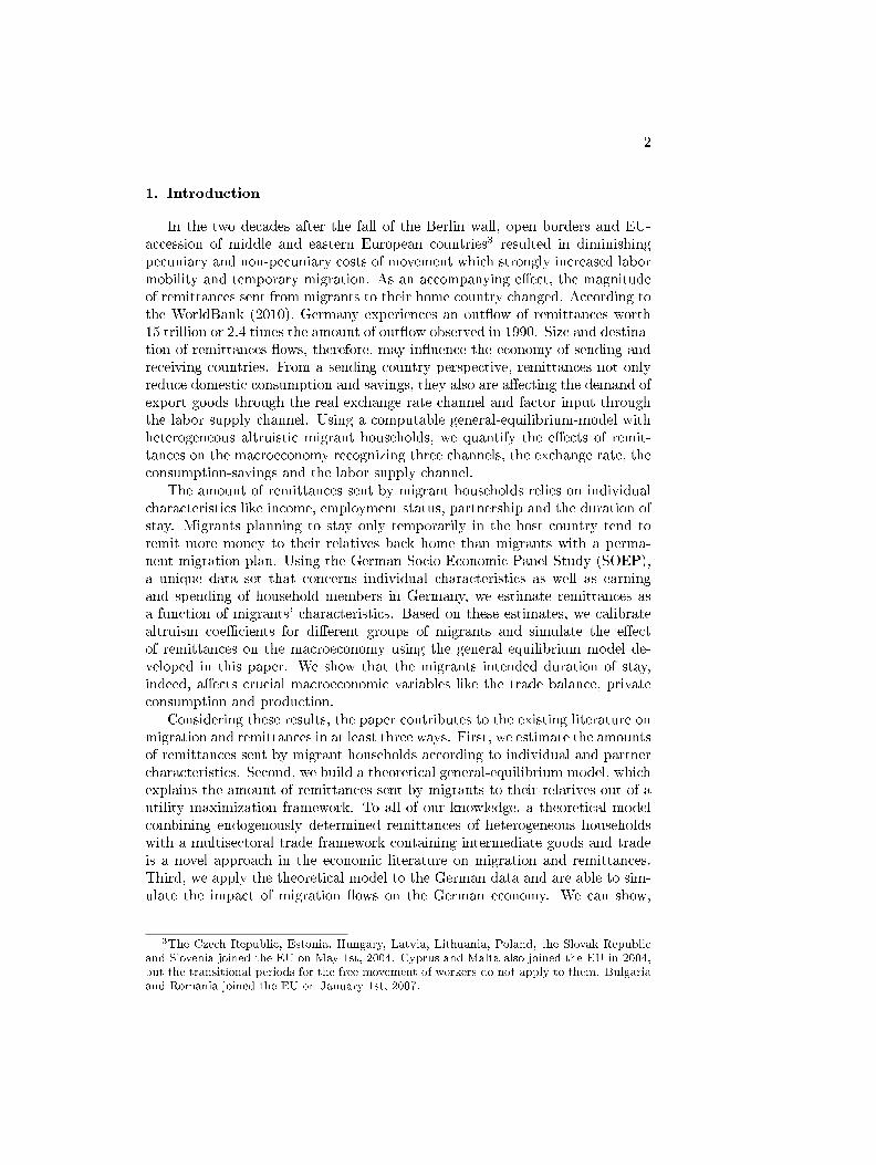
1. Introduction

In the two decades after the fall of the Berlin wall, open borders and EU-accession of middle and eastern European countries3 resulted in diminishingpecuniary and non-pecuniary costs of movement which strongly increased labormobility and temporary migration. As an accompanying e�ect, the magnitudeof remittances sent from migrants to their home country changed. According tothe WorldBank (2010), Germany experiences an out�ow of remittances worth15 trillion or 2.4 times the amount of out�ow observed in 1990. Size and destina-tion of remittances �ows, therefore, may in�uence the economy of sending andreceiving countries. From a sending country perspective, remittances not onlyreduce domestic consumption and savings, they also are a�ecting the demand ofexport goods through the real exchange rate channel and factor input throughthe labor supply channel. Using a computable general-equilibrium-model withheterogeneous altruistic migrant households, we quantify the e�ects of remit-tances on the macroeconomy recognizing three channels, the exchange rate, theconsumption-savings and the labor supply channel.

The amount of remittances sent by migrant households relies on individualcharacteristics like income, employment status, partnership and the duration ofstay. Migrants planning to stay only temporarily in the host country tend toremit more money to their relatives back home than migrants with a perma-nent migration plan. Using the German Socio-Economic Panel Study (SOEP),a unique data set that concerns individual characteristics as well as earningand spending of household members in Germany, we estimate remittances asa function of migrants' characteristics. Based on these estimates, we calibratealtruism coe�cients for di�erent groups of migrants and simulate the e�ectof remittances on the macroeconomy using the general equilibrium model de-veloped in this paper. We show that the migrants intended duration of stay,indeed, a�ects crucial macroeconomic variables like the trade balance, privateconsumption and production.

Considering these results, the paper contributes to the existing literature onmigration and remittances in at least three ways. First, we estimate the amountsof remittances sent by migrant households according to individual and partnercharacteristics. Second, we build a theoretical general-equilibrium model, whichexplains the amount of remittances sent by migrants to their relatives out of autility maximization framework. To all of our knowledge, a theoretical modelcombining endogenously determined remittances of heterogeneous householdswith a multisectoral trade framework containing intermediate goods and tradeis a novel approach in the economic literature on migration and remittances.Third, we apply the theoretical model to the German data and are able to sim-ulate the impact of migration �ows on the German economy. We can show,

3The Czech Republic, Estonia, Hungary, Latvia, Lithuania, Poland, the Slovak Republicand Slovenia joined the EU on May 1st, 2004. Cyprus and Malta also joined the EU in 2004,but the transitional periods for the free movement of workers do not apply to them. Bulgariaand Romania joined the EU on January 1st, 2007.

3

that migrants' behavior impacts crucial macroeconomic variables. Temporarymigrants more often send money back home and may consume goods there,whereas migrants with permanent migration plans send fewer remittances andconsume more goods in the host country. These di�erences a�ect the real ex-change rate between migrants' home and host country and change the sectoralstructure of production by triggering an opposite Dutch disease e�ect4; the re-mittances sent by migrants to their home country tend to bene�t the exportsectors of the host country.

The remainder of this paper is organized as follows. The next section sum-marizes the literature regarding the macroeconomic implications of remittances.The �macroeconomic model� section provides a theoretical outline of the gen-eral equilibrium model that is used in this study, whereas the �estimation andnumerical speci�cation� section describes our empirical strategy, in addition tothe calibration and simulation of the model. Finally, the last section concludesthe paper.

2. Related literature

The literature on remittances has primarily focused on the microeconomicaspects of this issue. In these models, migration is usually treated as an informalfamilial arrangement, with bene�ts that constitute risk diversion and the inter-generational �nancing of investments (Rapoport and Docquier, 2005). Remit-tances are a key element of such a contract and combine di�erent components,such as altruism, insurance, investment, inheritance, strategic considerationsand exchange.

The main focus of empirical studies are labor supply e�ects of relativesreceiving remittances. For Latin American economies, Fajnzylber and Lopez(2008), Funkhouser (1995) and Hanson (2007) report that remittances can re-duce the household labor supply. In contrast, Yang (2008) shows that remit-tances can also promote entrepreneurial activities by relaxing liquidity con-straints and, thus, increase the labor supply. A second strand of the empiricalliterature focuses on the amount of remittances sent by migrants. Dustmannand Mestres (2010) show, using the SOEP, that return plans are related to largechanges in remittances �ows. Using a small partial equilibrium model, Dust-mann (2000) shows that migrants with a temporary migration plan invest lessin speci�c human capital of the host country and tend to have higher costs ofleisure than migrants with a permanent migration plan. Temporary migrantstend to work more and in the �rst years since their arrival, this could result ina higher amount of remittances sent home.

4A situation where a country exports natural resources and harms its export sector by theappreciation of the currency is called a dutch disease phenomenon. In this article migrantssend remittances to their home country which depreciates the German currency and bene�tsits export sector. We call this phenomenon where a country sends transfers to another countryand bene�ts from depreciation an opposite dutch disease e�ect.

4

Macroeconomic models on remittances remain scarce; however, several stud-ies analyze the macroeconomic e�ects of remittances and the real exchange ratemovements in general equilibrium models.5 Following the macroeconometricliterature on remittances and Dutch disease e�ects6, Acosta et al. (2009) use adynamic stochastic general equilibrium model to address these e�ects. In theirmodel, the in�ow of remittances results in an exchange rate appreciation leavingexports with a loss in international competitiveness, which, in turn, can reducedemand and production of domestic produced goods.

The general equilibrium model that is developed in the following chapterdraws on several aspects of this literature. Remittances are endogenous in ourmodel because of the utility optimization of heterogeneous households, whereinwe integrate a microeconomic altruistic model, following Stark (1995), into ageneral equilibrium framework. This enables us to distinguish between di�er-ent groups of migrants and to estimate altruism coe�cients based on migrant'scharacteristics and the planned duration of stay. We use a multisector frame-work that calibrates openness on the basis of input-output tables from Eurostat.This method enables us to derive sector-speci�c e�ects and to take into accountthat in Germany, there is nearly no non-tradable sector. Furthermore, we cancapture the complex relationships of international production chains and thedemand for intermediate goods adding further insight into the appearance ofDutch-disease like e�ects. Finally, we include imperfect labor markets in ourtheoretical model to derive further insight into the labor market e�ects of re-mittances. To all of our knowledge this aspect is not covered in the literatureon the macroeconomics of remittances, yet.

3. The Model

In this section, we build a model that includes remittances, imperfect la-bor markets and multiple regions.7 This theoretical model is the basis for oursimulation exercise, which is intended to capture the relationship between mi-gration, remittances, the real exchange rate and the di�erent sectors of theeconomy. These relationships are then used to explain the emergence of anopposite Dutch disease e�ect.

The rational behind the migration decision is as follows. A member of ahousehold decides, with the agreement of the other household members, to mi-grate. The potential �ows of remittances are considered in this decision. Ac-cordingly, the utility of all household members, who remain in the home country

5An additional strand of literature uses IS-LM-BP like models and real business cyclemodels to analyze the implications of pro- and countercyclicity of remittances for stabilizationpolicy (e.g. Durdu and Sayan, 2010; Vargas-Silva, 2008). In these studies remittances areusually treated as a positive or negative exogenous shock on aggregate demand.

6Amuedo-Dorantes and Pozo (2004); Bourdet and Falck (2006) analyze the e�ects of re-mittances in macroeconometric models.

7The description of the model follows a contribution of Löfgren et al. (2001) who set someconventions for CGE modeling and reporting.

3.1 Households 5

or also migrated to other countries, is included in the migrant's utility function.An �altruism� coe�cient weights the amount of utility that is generated throughthe consumption of the household members who stay in foreign countries.

Therefore, migration increases the labor supply in an imperfect labor marketsetting, resulting in wage pressure and unemployment. Remittances changethe real exchange rate and lead to a change in production, depending on theopenness of the sectors of the economy.

3.1. Households

The model economy consists of a large number of households with in�nitelifespans, wherein a representative household seeks to maximize utility. Wefurther assume that some members of the household live abroad (e.g., in adistant source country). The utility of these distant members enters the utilityfunction of the migrant household in the host country, whereas the migrant'sutility enters the utility function of those household members remaining in thesource country. The utility function V of the migrant household and the utilityfunction of the relatives back home V ∗ take the following form

V (.) = βV ∗(.) + (1 − β)U(.), (1)

V ∗(.) = β∗V (.) + (1 − β∗)U∗(.). (2)

A household derives utility U (.) through the migrant's consumption of goodsQc and the utility of the relatives abroad V ∗(Q∗

c , γ∗c ). The parameter β can be

interpreted as the altruism coe�cient and γc, γ∗c denote a subsistence level of

consumption either of the migrant or of the relatives.The utility function of the members of the household who stay in a foreign

country evolves analogously. The two equations 1 and 2 are solved for V (.) with

V (Qc, Q∗c , γc, γ

∗c ) = (1 − α)U (Qc, γc) + αU∗ (Q∗

c , γ∗c ) . (3)

Where α = β(1−β∗)1−β∗β and 0 ≤ α ≤ 1

2 . The migrant's utility function is rewrittenas an indirect utility function.

V ∗ (Qc, Q∗c , γc, γ

∗c ) = (1 − α)U (Y − T ) + αU∗ (Y ∗ + T ) (4)

Maximizing the migrant's utility function for optimal remittances assumingthat relatives don't send transfers, T , yields.

− (1 − α)∂U

∂Qc+ α

∂U∗

∂Q∗c

≤ 0 (5)

Now, we use the inverse consumption function V (I). Because the migrantand his or her relatives have similar preferences by assumption, optimal remit-tances can be expressed in terms of disposable income Y .

T̄ = αY − (1 − α)Y ∗ (6)

3.1 Households 6

Consumers' preferences are speci�ed by a Stone-Geary function. The house-hold only derives utility from a part of total consumption Qc, which exceedsthe subsistence level of consumption γc. Utility maximization is subject to thedisposable income and the budget constraint of the household. The parameterαc denotes consumers preferences and pc the price of commodity c.

maxQc,γc

U(Qc, γc) =

n∏c=1

(Qc − γc)αc (7)

s.t.

(1 − tY − s)Y − T ≤n∑c=1

(1 + tQc)pcQc

with Qc > γc ≥ 0 and∑nc=1 αc = 1 for c = 1, 2, ...n and

Y =

n∑j=1

(1 − tKj)ijKj +

n∑j=1

(1 − tLj)wjLj + b · w ·

N −n∑j=1

Lj

.

The household earns a return ij via renting varieties j of capital Kj and wagewj in exchange for supplying varieties j of labor Lj to the �rm sector. Bothsources of income are subject to speci�c capital tKj or labor-related taxes tLj .Because of imperfect labor markets, it is likely that the labor supply N exceedsthe quantity of labor that is employed in the di�erent sectors of the economy.The household receives unemployment bene�ts which are a fraction of averageincome w for unemployed labor. The variable b denotes the correspondingreplacement rate. The available income for consumption spending I is de�nedas the household income Y net of income taxes tY Y , savings sY and remittancesT . The parameter tQc denotes commodity speci�c taxes.

We derive the tangency condition by di�erentiating the Lagrangian withrespect to its arguments, followed by equating the results to zero and thenrearranging them. This process can be used to derive the demand relations foreach good and obtain the expenditures on each commodity. The parameter αccan be taken as the marginal budget shares.

(1 + tQc)pQcQc = (1 + tQc)pQcγc + αc

(I −

n∑c=1

(1 + tQc)pQcγc

)(8)

The expenditure on each commodity can be divided into two parts. The �rstpart is the minimum required quantity to obtain a minimum subsistence levelof consumption. The second part depends on the available income that remainsafter buying the required quantities of each good. The budget constraint is onlymet if the sum of the exponents is equal to one. Deriving the income elasticityof commodity c is straightforward.

ξ(Qc, IH) =∂Qc∂I

· I

Qc=

αcI

(1 + tQc)pQcQc(9)

3.2 Firms 7

Following Saito (2004), we derive a Frisch parameter φ from the demandrelationship of the commodities to capture the average elasticity of substitution.Therefore, we solve the Lagrange function for the Lagrangian λ and calculate theexpenditure elasticity of the marginal utility of expenditure, which is the Frischparameter. This elasticity can be used to calibrate γc, which is the minimumrequired quantity of a good that the representative household requires.

φ =dλ

dI· Iλ

= − I

(I −∑ni=1 pQcγc)

(10)

3.2. Firms

Both �nal and intermediate goods are supplied in competitive domestic mar-kets. Factor demands are also determined in a perfectly competitive fashion. Arepresentative �rm of an activity a solves a cost minimization problem to de-termine the factor demand that is subject to a nested linear-homogeneous CESproduction function. In the �rst nest, each �rm combines the gross value addedVa and intermediate goods Ia to produce the gross output QDa. Depending onthe production structure of the economy, gross output can be divided into dif-ferent goods QDaφca = QDc, with φac as share parameter. The parameters pV aand pIa denote the internal price of value added and the price for intermediategoods, respectively.

minVa,Ia

ΓQDa (Va, Ia) = pV aVa + pIaIa (11)

s.t.

QDa = (µaV−ρaa + (1 − µa)I−ρaa )

−1ρa

Value added is generated by using capital K and labor L in the second nest ofthe production function. The parameter ρ denotes the elasticity of substitutionamong the di�erent factors, A denotes factor productivity, and µ can be taken asa share parameter of production. The corresponding parameters ρV , ρLa,, ρKaand µV a, µLa, µKa exist in each nest of the production function.

The factors of production are rewarded with the aggregate interest rate r oncapital and the aggregate wage w on labor. The �rm minimizes its total costsΓ in every nest of the production function.

minKa,La

ΓV a (Ka, La) = raKa + waLa (12)

s.t.

Va = AaµV a(µV aK

−ρV aa + (1 − µV a)L−ρV a

a

) −1ρV a

Finally, in the third nest, the �rm minimizes the two cost functions ΓLaj ,ΓKajwith regard to two production functions, which aggregate the varieties of capitaland labor.

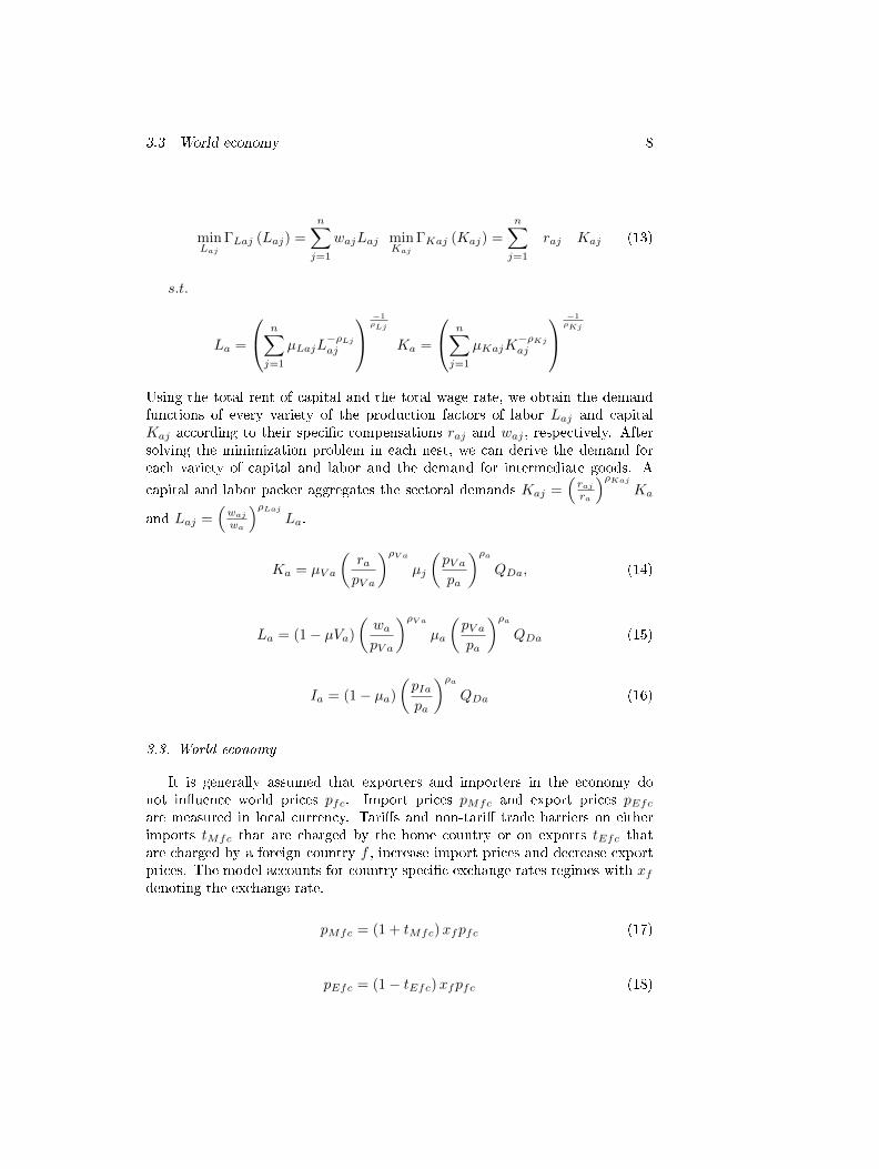
3.3 World economy 8

minLaj

ΓLaj (Laj) =

n∑j=1

wajLaj minKaj

ΓKaj (Kaj) =

n∑j=1

raj Kaj (13)

s.t.

La =

n∑j=1

µLajL−ρLjaj

−1ρLj

Ka =

n∑j=1

µKajK−ρKjaj

−1ρKj

Using the total rent of capital and the total wage rate, we obtain the demandfunctions of every variety of the production factors of labor Laj and capitalKaj according to their speci�c compensations raj and waj , respectively. Aftersolving the minimization problem in each nest, we can derive the demand foreach variety of capital and labor and the demand for intermediate goods. A

capital and labor packer aggregates the sectoral demands Kaj =(rajra

)ρKajKa

and Laj =(wajwa

)ρLajLa.

Ka = µV a

(rapV a

)ρV aµj

(pV apa

)ρaQDa, (14)

La = (1 − µVa)

(wapV a

)ρV aµa

(pV apa

)ρaQDa (15)

Ia = (1 − µa)

(pIapa

)ρaQDa (16)

3.3. World economy

It is generally assumed that exporters and importers in the economy donot in�uence world prices pfc. Import prices pMfc and export prices pEfcare measured in local currency. Tari�s and non-tari� trade barriers on eitherimports tMfc that are charged by the home country or on exports tEfc thatare charged by a foreign country f , increase import prices and decrease exportprices. The model accounts for country speci�c exchange rates regimes with xfdenoting the exchange rate.

pMfc = (1 + tMfc)xfpfc (17)

pEfc = (1 − tEfc)xfpfc (18)

3.3 World economy 9

3.3.1. Export sector

The �rm has a choice between selling a given amount of its product in thehome marketQDDc or to export it Ec to foreign countries f that may be inside oroutside of the EU. A �rm maximizes its revenues based on a CET transformationfunction considering the prices of goods for export pEc and for domestic salespDc. The parameter ρ indicates the elasticity of the transformation, whereasthe parameter γ can be seen as the share parameter of the CET function. Theparameter awc accounts for di�erent levels of technology.

maxEc,QDDc

ΓQc (Ec, QDDc) = pEcEc + pDcQDDc (19)

QDc = aDc[γTcE

−ρDcc + (1 − γTc)Q

−ρDcDDc

]− 11−ρDc (20)

We can determine the destination of exports by maximizing the revenuefunction based on a sub-CET function. The �rm receives revenues from sellinggoods Efc to di�erent countries recognizing the corresponding export pricespEfc. The parameter γWc is a shift parameter, whereas ρWc accounts for thesubstitution elasticity of di�erent destinations within the sub-CET function.

maxEfc

ΓEfc (Efc) =

o∑f=1

pEfcEfc (21)

Ec = aWc

o∑f=1

γWcE−ρWc

fc

11−ρWc

(22)

After setting up the Lagrangian and the re-parameterization of ρDc = (1/σDci)−1, we can derive the optimum supply for the home QDDc and the world marketsEc.

QDDc = (1 − γDc)σTcp−σTcDc

[γσTcTc p

1−σTcEc + (1 − γTc)

σTc p1−σTcDc

] σDc1−σDc QDc/aDc

(23)

Ec = γσDcDc pE−σDcc

[γσDcDc pEc+ (1 − γDc)

σDc p1−σDcDc

] σDc1−σDc QDc/aDc (24)

3.3.2. Import sector

A wholesaler minimizes the costs of the intermediate and �nal goods bycombining di�erent sources of goods with an Armington function ΓMc. TheArmington function implies that goods are di�erentiated among countries; how-ever, goods from di�erent countries can be close substitutes. In the �rst nestof the Armington function, the wholesaler chooses between imported goods Mc

with price pMc and domestically produced goods QDDc with price pDc. The

3.4 Government 10

parameter γAc is the shift parameter of the Armington function, and ρAc is theelasticity of substituting goods from di�erent source countries.

minMc,QDDc

ΓMc (Mc, QDDc) = pMcMc + pDcQDDc (25)

s.t.

Qc = aAc[γAcM

−ρAcc + (1 − γAc)Q

−ρAcDDc

] 11−ρAc (26)

In the second nest of the Armington function ΓMfc, the wholesaler minimizesits costs by choosing the optimum combination of the di�erent commoditiesMfc with the price pMfc from di�erent countries. The parameter γSc is a shiftparameter, and ρSfc is the elasticity of substituting import goods from di�erentsource countries. The parameter aSc denotes the di�erent levels of technologyin the di�erent sectors.

minMfc

ΓMfc (Mfc) =

o∑f=1

pMfcMfc (27)

s.t.

Mc = aSc

o∑f=1

γScM−ρSfcfc

11−ρSfc

(28)

We can, thus, derive the demand for imports and domestic production inthe home market.

QDc = (1 − γTc)σAcp−σAcDc

[γσAcAc p

1−σAcMc + (1 − γAc)

σAc p1−σAcDc

] σAc1−σAc Qc/aAc

(29)

Mc = γσAcAc p−σAcMc

[γσAcAc p

1−σAcMc + (1 − γAc)

σAc p1−σAcDc

] σAc1−σAc

Qc/aAc (30)

The demand for imported goods from di�erent countries is subject to a sub-Armington function, which yields the demand for imported goods according todi�erent sources:

Mfc = γσScSc p−σScfc

o∑f=1

γσScSc p−σScfc

σSc1−σScMc/aSc (31)

3.4. Government

The government levies taxes on labor8 and capital usage, income and con-sumption. Additionally, it collects tari�s. Consequently, the government rev-enue function YG takes the following form:

8Please note that we assign public social security services to the state sector. Social securitycontributions are therefore treated as taxes and insurance payments as transfers.

3.4 Government 11

YG =

n∑c=1

tQcQcpDc +

o∑f=1

tMfcxfpfcMfc

+

n∑a=1

n∑j=1

(tKjKajraj + tLjLajwaj) .

(32)The government spends its income on consumption QGc, government savings

SG, sector related subsidies to �rms and households Za, and unemploymentbene�ts.

YG = (w · b) (N −n∑j=1

Lj) +

n∑a=1

paZa +

n∑c=1

pcQGc + SG (33)

With respect to consumption, the government maximizes a Stone-Gearyutility function that is subject to a budget constraint, which is derived from 32and 33.

maxCGc,γGc

UG =∏c

(QGc − γGc)αGc (34)

We can derive government expenditures for consumption using a method thatis similar to that used for the household sector. We assume that the state sectoris not subject to VAT payments. The consumption of the government is splitinto subsistence consumption γGc and consumption for utility αGcQGc.

pcQGc = pcγGc + αGcpcQGc (35)

In addition to consumption and transfers, the state sector, like the �rmsector, produces public goods using intermediate goods IGa, labor LGa andcapital KGa. The state sector minimizes costs ΓQGa using a CES productionfunction QGa.

minVGa,IGa

ΓQGa (VGa, IGa) = pGV aVGa + pIaIGa (36)

s.t.

QGa = (µGaV−ρGaGa + (1 − µGa)I−ρGaGa )

−1ρGa (37)

We can then derive the demand for these three kinds of inputs. We assumethat the state sector chooses inputs in terms of varieties of labor and capital ina way that is similar to private companies; however, the state does not exportgoods but, instead, buys aggregate intermediate goods from wholesalers.

KGaj = µGV a

(rajra

)ρGKaj ( rapV a

)ρGV aµGV a

(pV apa

)ρGaQGa (38)

LGa = (1 − µGV a)

(wapV a

)ρGV aµGV a

(pV apa

)ρGaQGa (39)

3.5 Equilibrium conditions 12

IGa = (1 − µGa)

(pIapa

)ρGaQGa (40)

3.5. Equilibrium conditions

We complete the model using the respective equilibrium conditions for thefactor markets, goods markets and foreign markets. The goods markets are inequilibrium if domestic and foreign productions equal the household, govern-ment and intermediate goods demand.

pcQGc+(1 + tQc) pcQc+pc (Ic + IGc) = pDcQDDc+

o∑f=1

(pMfcMfc)−o∑

f=1

(pEfcEfc)

(41)

The capital markets are in equilibrium if supply KS equals demand and ifthe labor markets are subject to a wage-setting curve ~ and, therefore, are indisequilibrium. The �rms take the bargained wages as a given and adjust theirlabor demand.

n∑j=1

(Kj +KGj) = KS (42)

w = ~

N −n∑a=1

n∑j=1

(Laj + LGj)

(43)

The foreign sector is in equilibrium if imports, exports and foreign savingsare equal in terms of payment balances.

o∑f=1

n∑c=1

pMfcMfc =

o∑f=1

n∑c=1

pEfcEfc +

o∑f=1

Sf (44)

4. Estimation and numerical speci�cation

The general equilibrium problem that was described in our theoretical modelfeatures characteristics that can be formulated as mixed complementarity prob-lem (MCP). Using this formulation we are able to apply the model to the datafor simulation purposes. The calibration of the model is done using most re-cent input-output matrices from Eurostat, which provide data on the Germaneconomy in 2007. The altruism coe�cient, however, is calibrated on basis ofour estimates on the remittance behavior of migrants in Germany. We use theSOEP to estimate remittances according to migrants' individual characteristicsand family relations.

4.1 Data and Estimation 13

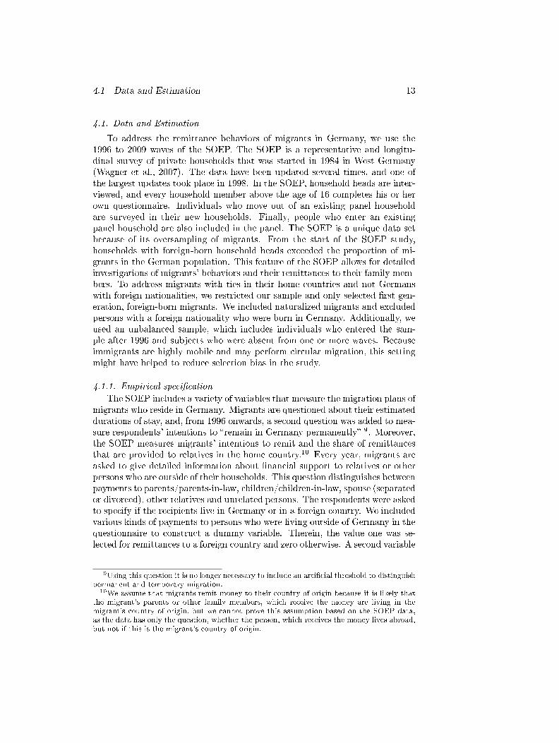
4.1. Data and Estimation

To address the remittance behaviors of migrants in Germany, we use the1996 to 2009 waves of the SOEP. The SOEP is a representative and longitu-dinal survey of private households that was started in 1984 in West Germany(Wagner et al., 2007). The data have been updated several times, and one ofthe largest updates took place in 1998. In the SOEP, household heads are inter-viewed, and every household member above the age of 16 completes his or herown questionnaire. Individuals who move out of an existing panel householdare surveyed in their new households. Finally, people who enter an existingpanel household are also included in the panel. The SOEP is a unique data setbecause of its oversampling of migrants. From the start of the SOEP study,households with foreign-born household heads exceeded the proportion of mi-grants in the German population. This feature of the SOEP allows for detailedinvestigations of migrants' behaviors and their remittances to their family mem-bers. To address migrants with ties in their home countries and not Germanswith foreign nationalities, we restricted our sample and only selected �rst gen-eration, foreign-born migrants. We included naturalized migrants and excludedpersons with a foreign nationality who were born in Germany. Additionally, weused an unbalanced sample, which includes individuals who entered the sam-ple after 1996 and subjects who were absent from one or more waves. Becauseimmigrants are highly mobile and may perform circular migration, this settingmight have helped to reduce selection bias in the study.

4.1.1. Empirical speci�cation

The SOEP includes a variety of variables that measure the migration plans ofmigrants who reside in Germany. Migrants are questioned about their estimateddurations of stay, and, from 1996 onwards, a second question was added to mea-sure respondents' intentions to �remain in Germany permanently� 9. Moreover,the SOEP measures migrants' intentions to remit and the share of remittancesthat are provided to relatives in the home country.10 Every year, migrants areasked to give detailed information about �nancial support to relatives or otherpersons who are outside of their households. This question distinguishes betweenpayments to parents/parents-in-law, children/children-in-law, spouse (separatedor divorced), other relatives and unrelated persons. The respondents were askedto specify if the recipients live in Germany or in a foreign country. We includedvarious kinds of payments to persons who were living outside of Germany in thequestionnaire to construct a dummy variable. Therein, the value one was se-lected for remittances to a foreign country and zero otherwise. A second variable

9Using this question it is no longer necessary to include an arti�cial threshold to distinguishpermanent and temporary migration.

10We assume that migrants remit money to their country of origin because it is likely thatthe migrant's parents or other family members, which receive the money are living in themigrant's country of origin, but we cannot prove this assumption based on the SOEP data,as the data has only the question, whether the person, which receives the money lives abroad,but not if this is the migrant's country of origin.

4.1 Data and Estimation 14

measures the exact amount of the remitted money. Here, we use the logarithmof the remittance amounts in Euro 11. To measure the migrants' individual char-acteristics and their ability to send money home, we used information regardingthe age of the individual at the time of immigration, years since migration, yearsof education, nationality, income, gender and marital and employment status.We also included information on the number of children who were under the ageof 16 and were living in the host country household. In addition to the migrant'scharacteristics, we included the characteristics of the migrant's partner, regard-less of his or her migrational background. This approach allows us to draw amore complete picture of the household. Speci�cally, we used information onthe partner's income, years of education, nationality and desire to permanentlyremain in Germany.

Following Dustmann and Mestres (2010), we estimate the impact of thesecharacteristics on the probability of remitting and the remitted amounts usingsimple probit and OLS models. As Dustmann (2000) has demonstrated, con-ventional �xed e�ect models and forward orthogonal �xed e�ects regressions(Arellano and Carrasco, 2003) might be biased. Our regressions are of the fol-lowing type:

Yit = β0 + β1 ∗ temp+ β2 ∗ par + β3 ∗Xit + uit (45)

Yit = β0 + β1 ∗ temp+ β2 ∗ par+ β3 ∗Xit + β4 ∗ partempit + β5 ∗Zit + uit (46)

Y measures either the probability that a person i will remit money to his orher country of origin over time t or the amount remitted. The �rst speci�cationof our model described in equation eq:Estimation equation probit takes onlyindividual characteristics into account, while the second speci�cation estimatesthe probability and the amount of money a person remits based on individualas well as on the partner's characteristics . The variable �temporary� is one ofour primary variables of interest, and it is speci�ed as a dummy variable thattakes the value one if an individual intends to return to his or her home countryand zero otherwise. Using this dummy variable, we can measure the impactof migrants' intentions to return to their country of origin on the probabilityof them remitting and the remittance amounts. The second dummy variable,which is speci�ed in our equation as partner, indicates the presence of a partnerin the migrant household in the host country. We do not distinguish betweenmarriage and cohabitation. Other individual characteristics, such as educationor income, are covered by the parameter X.

In a second speci�cation (see equation 46), we included the partner's char-acteristics in the evaluations of individuals who live with partners, as shownin the formula for the intention of the partner to stay in Germany temporarily(partemp). These data are included as an interaction term with the partner

11The dependent variable takes the following structure: log(remittances in Euro + 1).

4.1 Data and Estimation 15

variable. For single migrants, the variable is zero and does not a�ect remittancebehaviors. For migrants with partners, this variable indicates the in�uence ofthe partner's characteristics on the probability of remitting and the remittedamounts. Additional partner characteristics enter the equations by the param-eter Z.

4.1.2. Descriptive evidence

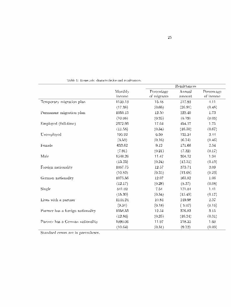
Table 1 provides descriptive information on the percentage of individuals whoremit, the amount of money they remit, their monthly earnings and, �nally, thepercentage of migrants' annual incomes that are spent on remittances. Thelast variable is calculated using the migrants' average monthly incomes and theaverage amount of monthly remittances. At �rst glance, we can observe signi�-cant di�erences with regard to individual characteristics. Remittances seem tobe a luxury good, and the probabilities of remitting and remittance amountssubstantially di�er between employed and unemployed migrants. Nearly 18 per-cent of the migrants who had full time jobs sent money to their home country,whereas only 6.5 percent of the migrants who were unemployed or otherwise sentmoney. Moreover, the remittance amounts were more than three times higheramong the employed participants than among the unemployed participants.

Table 1 about here

Interestingly, �nancial factors are not the only attributes that in�uence theprobability of remitting and the remitted amounts. Nationality and future plansregarding the duration of the stay seem to play an important role in remittances.A total of 15 percent of the migrants who intended to leave Germany sent moneyhome compared with 12.5 percent of those who intended to permanently stayin Germany. The group di�erences are smaller when we compare migrants withforeign and German nationalities. A total of 12.5 percent of migrants who hadforeign nationalities sent money home, whereas only 12 percent of migrantswith German citizenship did so. We found similar results for migrants whosepartners had foreign (12.5 percent) or German citizenship (12 percent). Fur-thermore, the amounts of money that were remitted by migrants with Germanor foreign citizenship (as well as for migrants with German or foreign part-ners) di�ered. Additionally, we observed di�erences between male and femalemigrants. Females reported a lower probability of remitting in comparison totheir male counterparts. In addition, the men in the sample, on average, sentmore money to their home country; however, when we measure remittances asa percentage of annual income, the picture changes, that is, the women sent ahigher percentage of their annual income abroad. Overall, those migrants whointend to temporarily stay in Germany are not only more likely to send thelargest amounts of money abroad, but they also send a higher percentage oftheir annual income. Temporary immigrants remit, on average, more than fourpercent of their annual income, whereas permanent migrants remit less thantwo percent of their income.

4.1 Data and Estimation 16

4.1.3. Estimation results

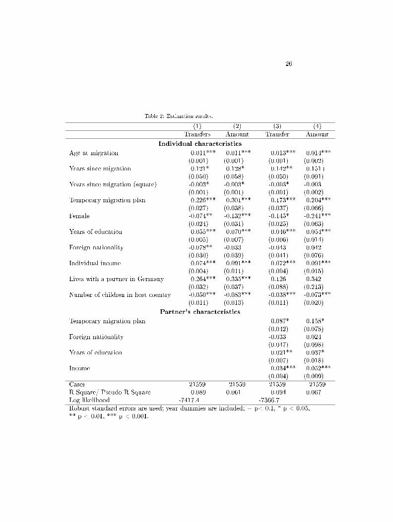
The descriptive statistics in Table 1 that were identi�ed in this study indicatestrong di�erences in migrants' remittance behaviors. To identify the likelihoodof remitting and the amount of money remitted, we tested two model speci-�cations using probit and OLS regressions so as to create four models. Thespeci�cations of these models di�er with regard to the inclusion of speci�c char-acteristics that are related to the migrants' partners. Therefore, columns threeand four in Table 2 include additional partner characteristics. This approachallows us to account for partners' in�uences on the probability of remitting andthe remitted amounts. A partner may in�uence the decision to remit throughdi�erent mechanisms. First, a partner's salary might substantially increase thehousehold's income and, thus, the ability to remit. Second, the decision to re-turn to the home country may be a household decision. Therefore, we includeinformation on the partner's nationality, his or her migration plans regardingthe duration of the stay in Germany, education and income.

Table 2 about here

In all of our models, the variable identifying a temporary stay in Germanyshows a strong and positive e�ect on the probability of remitting and the re-mitted amounts. All of our models indicate that the age at migration positivelyimpacts the likelihood to remit and the remittance amount. Persons who mi-grate at an older age might have stronger ties with their country of origin andare, therefore, more likely to remit and send larger amounts of money home.Moreover, the time that is spent in the host country also in�uences the proba-bility of remitting and the remitted amounts. All Models demonstrate a clearconcave relationship between the time spent in the host country and the prob-ability of remitting and the remitted amounts. The probability of remittingand also the amount remitted increases in the �rst years after arriving in thehost country according to our �rst two models. In Model 1, after 23 years ofresidence in the host country, the probability of sending money declines again(in Model 2, the remitted amount decreases after 20 years in the host country).Our regressions also indicate that like the migrant's future plans (temporary vs.permanently), the partner's migration plans signi�cantly in�uence the probabil-ity of remitting and the remitted amounts. This result supports the correlationof migration plans with remittances that is depicted in Table 1. In Model 4,the remittance amount increases by 20 percent when migrants have a temporarymigration plan and decreases as a function of the duration of stay by 1.5 percentper year.

In all of our models, education positively impacts the probability of remit-ting and the remitted amounts. More educated migrants might more e�ectivelyintegrate into the new labor market e.g., they might know the language or beable to learn it quickly. Better workforce integration and better education re-sult in higher wages. In turn, more educated migrants can a�ord to send larger

4.2 Simulation 17

remittances. Finally, individual income has a positive and highly signi�cant im-pact on both dependent variables. With every percent increase in the migrant'searnings, the amount of remittances increases by 0.09 percent and the likeli-hood to remit money increases by 0.07 percent. This �nding con�rms the Starkmodel's implication that sending money home depends on a migrant's income.Remittances can be interpreted as a kind of luxury good that shares increasingdisposable income with other forms of consumption.12

A higher number of children in the host country reduces the amount ofmoney that is sent and the likelihood of remitting. Although the e�ect isweaker in Models 3 and 4, which control for partner characteristics, individ-uals with children in their host countries are, on the one hand, more likely tohave their immediate family with them and have, therefore, a lower altruismcoe�cient for their household members in their home country. On the otherhand, children generally reduce per capita household income, which results inlower remittances.

Our inclusion of the variables that relate to the migrants' partners indicatesthat the partner's employment status positively in�uences the probability ofremitting and the remitted amounts. Both Models 3 and 4 show that partners'migration plans are also important to remittance behaviors. Although the e�ectis weaker than the individual e�ect, it is stable and signi�cant. Temporarymigrants who live with a partner in Germany who himself or herself intends toreturn to his or her home country are 26 percent more likely to remit moneyand remit 36 percent more in comparison to a single migrant who intends topermanently live in the host country.

4.2. Simulation

We follow Böhringer et al. (2003) by specifying the general equilibrium in theCGE model as a mixed complementarity problem (MCP). According to Cottleet al. (2009) and Rutherford (1995), such a problem can be best solved using thePATH solver.13In the MCP approach, equilibrium conditions are formulated asweak inequalities and conditions of complementary slackness between variablesand equilibrium conditions. The model was set up as an Arrow-Debreu economywith n = 16 commodities and m = 16 domestic industries. In total, there are2 agricultural industries, 4 manufacturing industries and 10 service industries.Each commodity corresponds to an industry.

4.2.1. Calibration

The economic relationships in the macroeconomic model are calibrated usinga symmetric social accounting matrix. The social accounting matrix builds on

12In our model we use a Stone-Geary utility function to re�ect these empirical �ndings.13The Path solver is based on the Newson-Raphson method. According to the General Al-

gebraic Modeling System (GAMS), the PATH solver combines a number of the most e�ectivevariations, extensions, and enhancements to increase the e�ciency of �nding new approxima-tions with this solution method.

4.2 Simulation 18

the input-output matrices that are provided by Eurostat in 2007. We tookinformation on consumption by household type from the German microcensusof the same year and data on the replacement rate of di�erent kinds of labor.

The SAM satis�ed the model's microeconomic equilibrium conditions andwas used to calibrate most of the model's parameters. Nevertheless, we couldnot calibrate the elasticity of substitution between capital and labor and theArmington elasticities. Thus, we used standard substitution elasticities andestimates of the Armington elasticities based on Saito (2004) 14. We calibratedthe altruism coe�cients of households based on our econometric estimates fromthe SOEP data-set.

Additionally, we took the elasticities between the unemployment and wagerates from the empirical study of Brücker et al. (2009). The wage setting curve,which describes the bargaining of trade unions and employers, has an elasticityof -0.08 for Germany.

4.2.2. Scenarios

Ever since the 1950s, migration is a key driving force for population growth inGermany. The migration balance is positive in most years at a yearly amountof between 129.000 and 354.000 people. In the last �ve years, however, themigration balance was declining and not always positive. There are at leasttwo reasons for this phenomenon. The net-out�ow of people with a Germancitizenship is rising and the number of ethnic German immigrants from formersocialist countries is falling. In the next years it is expected that the migrationbalance is rising again. Favorable economic conditions, open labor marketsand an increasing demand in skilled workers should increase immigration in thenext years. Emigration, on the other hand, should decrease. The nature of theaging process in Germany reduces the cohort of people most likely to leave thecountry. Taking these considerations into account, the Federal Statistical O�cein Germany is expecting that migration in the next decade will be between100.000 and 200.000 migrants after a short period of still moderate migrationin the next few years.

Table 3 about here

Remittances, in all scenarios of our model, were calibrated on the basisof our empirical estimates. When we accounted for individual characteristics(e.g., age, years since migration and intention to stay), we derived the altruismcoe�cient and the remittance amounts sent home. Speci�cally, if new migrantsare assumed to behave similarly to migrants who arrived in Germany in theyears leading up to 2007, a yearly in�ow of between 100.000 and 200.000 peoplein the next years would increase remittances by approximately 716 million to 1.4

14We used a variety of alternative substitution elasticities provided for sensitivity analysis.

4.2 Simulation 19

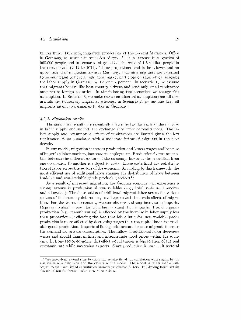
billion Euro. Following migration projections of the Federal Statistical O�cein Germany, we assume in scenarios of type A a net increase in migration of900.000 people and in scenarios of type B an increase of 1.6 million people inthe next decade (2012 to 2021). These projections tend to be a lower and anupper bound of migration towards Germany. Incoming migrants are expectedto be young and to have a high labor market participation rate, which increasesthe labor supply in Germany by 1.4 or 2.2 percent. In scenario 1, we assumethat migrants behave like host country citizens and send only small remittanceamounts to foreign countries. In the following two scenarios, we change thisassumption. In Scenario 3, we make the counterfactual assumption that all newarrivals are temporary migrants, whereas, in Scenario 2, we assume that allmigrants intend to permanently stay in Germany.

4.2.3. Simulation results

The simulation results are essentially driven by two forces, �rst the increasein labor supply and second, the exchange rate e�ect of remittances. The la-bor supply and consumption e�ects of remittances are limited given the lowremittances �ows associated with a moderate in�ow of migrants in the nextdecade.

In our model, migration increases production and lowers wages and becauseof imperfect labor markets, increases unemployment. Production factors are mo-bile between the di�erent sectors of the economy; however, the transition fromone occupation to another is subject to costs. These costs limit the redistribu-tion of labor across the sectors of the economy. According to this framework, themost e�cient use of additional labor changes the distribution of labor betweentradable and non-tradable goods producing sectors.15

As a result of increased migration, the German economy will experience astrong increase in production of non-tradables (e.g., hotel, restaurant servicesand education). The distribution of additional migrant labor across the varioussectors of the economy determines, to a large extent, the trade e�ects of migra-tion. For the German economy, we can observe a strong increase in imports.Exports do also increase, but at a lower extend than imports. Tradable goodsproduction (e.g., manufacturing) is a�ected by the increase in labor supply lessthan proportional, re�ecting the fact that labor intensive non-tradable goodsproduction is more a�ected by decreasing wages than the capital intensive trad-able goods production. Imports of �nal goods increase because migrants increasethe demand for private consumption. The in�ow of additional labor decreaseswages and should dampen �nal and intermediate good prices within the econ-omy. In a one sector economy, this e�ect would trigger a depreciation of the realexchange rate while increasing exports. Since production in our multisectoral

15We have done several runs to check the sensitivity of the simulation with regard to theelasticities of substitution and the closure of the model. The model is rather stable withregard to the elasticity of substitution between production factors. The driving forces withinthe model are the factor market closure equations.

4.2 Simulation 20

framework is increased basically in non-tradable goods sectors, e�ects on thereal exchange rate are limited. By assumption, world prices are not a�ected bythe increase in demand of consumption goods. However, the more than propor-tional increase in non-tradable goods production results in an appreciation ofthe real exchange rate and a worsening of the trade balance.

The out�ow of remittances has a counter-directional e�ect on exchange ratesand the trade balance. The out�ow of �nancial �ows a�ects the trade balancethrough the depreciation of the real exchange rate. The depreciation, given �xedworld prices, accelerates foreign demand and increases production, especially inthe manufacturing sector, which exports most of its products. The e�ect onprivate consumption is ambivalent and relies on the elasticity of foreign demandwith respect to price changes of export goods. On the one hand, remittancesreduce private consumption directly by re-channeling resources from privateconsumption to private remittances. On the other hand, private consumptionincreases because of lower unemployment and higher wages.

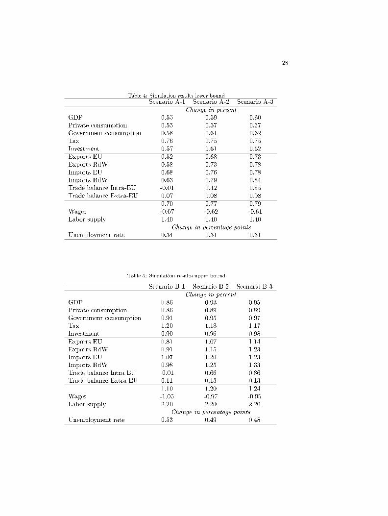
Table 4 and 5 about here

Table 4 and 5 report the percentage change of macroeconomic variables andtables 6 and 7 the percentage change of economic activities for the upper andlower bound of migration projections. The labor force increases in the lowerbound of migration projections by 1.4 (table 4 and 6) and in the upper boundby 2.2 percent (table 5 and 7). In both of the two tables, we report three sce-narios, where it is assumed that migrants behave like natives or have either atemporary or have a permanent migration plan. The migrant's plan in�uencesthe altruism of migrants with regard to relatives living abroad. If altruismis high, migrants tend to send more remittances. In the �rst scenario, wheremigrants act like natives, the additional labor force results in an increase inGDP by 0.55 percent. By assumption, the capital endowment remains constant.16Relative factor prices are changing because of the additional supply of la-bor. Wages are decreasing by 0.67 percent and the rate of return is increasingfor capital by 0.7 percent. Because of the imperfect labor market setting, theunemployment rate is increasing by 0.37 percentage points.

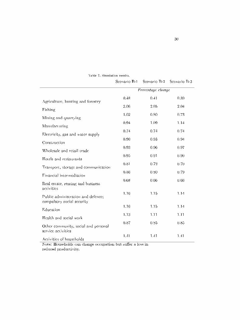
Table 6 and 7 about here

The change in relative prices in�uences the production of economic activitieswithin the economy. Activities with a high share of labor and a low share of

16In our sensitivity analysis, we relax this assumption. The trade e�ects remain ratherunchanged, but, as capital is no restricting factor anymore, the increase in production is morepronounced in this kind of speci�cation.

21

capital are increasing production by a bigger margin than activities with a lowshare of labor. Especially activities producing non-tradable goods, like the ac-tivity of household sector, can increase production by a more than proportional0.9 percent.

The planned duration of stay increases GDP for both kinds of migrationplans by 0.04 or 0.05 percent respectively compared to the �rst scenario wheremigrants send only small amounts of remittances like natives. The increase inGDP relies on a strong 0.16 (0.18) percent increase in intra-EU exports. Thetrade balance improves resulting in a higher production of activities produc-ing tradable goods. The increase in manufacturing is strongest with 0.1 (0.12)percent, followed by a 0.02 (0.03) percent increase in construction which, inGermany, is strongly interrelated with the manufacturing sector. The activi-ties producing non-tradable goods cannot increase production like the activitiesof households sector, or they lose like hotels and restaurant and public goodsactivities (e.g. public administration, health or social care and education).

As we have shown in our econometric estimates, temporary migrants donot only send more money home, they have also a higher probability to remitthan their counterparts intending to stay permanently in the host country. Thisresults in an additional 20 to 30 percent of remittances �ows observed in thesecond scenario. In our simulations, the counterfactual assumption that all mi-grants have temporary migration plans results in an increase in intra-EU andextra-EU exports of 0.05 percent (approximately EUR 1.3 trillion) and extra-EU exports of 0.04 percent, GDP increases by an additional 0.01 percent andmigrant households tend to reduce the demand for goods. Because of the realexchange rate appreciation, intra-EU imports increase only slightly (0.02 per-cent), and extra-EU imports, not a�ected by the exchange rate e�ect, increaseby 0.05 percent. In sum, migrants with temporary migration plans slightlyimprove Germany's trade balance. The distribution of production in the dif-ferent sectors of the economy tends to re�ect the redistribution of productiontowards tradable goods. The manufacturing sector increases production by 0.03percent, whereas most service sectors keep production constant. In sum, re-mittances tend to bene�t the tradable goods sectors by a depreciation of thereal exchange rate triggering an e�ect similar to the well known Dutch diseasephenomenon. In this case, the sending country of remittances is able to bene�tfrom a real exchange rate e�ect leaving the export industry better o�.

5. Conclusions

In the next decade, migration to Germany is likely to increase because ofan aging society and more prosperous economic conditions. Like in the UK,concerns about increasing remittances trigger fears that migration would harmthe domestic economy. Among host country citizens, the out�ow of remittancesis often seen as an out�ow of purchasing power; however, as we have shown inour simulation study, remittances are likely to bene�t the German economy. Anincrease in remittances results in a higher share of exports, an improvement ofthe trade balance and an increase in GDP. For the service sectors, remittances

22

are less favorable. The shift in migrants' consumption towards remittancesreduces demand of service goods from the host country.

As our calculations demonstrate, remittance �ows are determined by mi-grants' plans for temporary or permanent migration. Temporary migrants arelikely to remit more than twice the amount of money in comparison to per-manent migrants. We established three di�erent scenarios to investigate thesedi�erences. In the �rst two scenarios, migrants either had temporary or per-manent migration plans, whereas in the third scenario, migrants only sent asmall amount of remittances, as is done by the German native population. Ata �rst glance, the macroeconomic e�ects of changing from one counterfactualto another seem narrow. When we move from the temporary scenario to thepermanent scenario, the simulation results show an increase in exports of 0.05percent and an increase in GDP of 0.01 percent, only. Nevertheless, the remit-tances in this model are worth 380 billion Euro for a ten years period. Giventhe small scale of these remittances, the e�ects of our simulation are consid-erable. An open economy like Germany's seems to bene�t from an oppositeDutch disease e�ect, in which the competitiveness of the tradable goods sectorsincrease.

23

References

Acosta, P. A., Lartey, E. K. K., Mandelman, F. S., 2009. Remittances and thedutch disease. Journal of International Economics 79 (1), 102�116.

Amuedo-Dorantes, C., Pozo, S., 2004. Workers' remittances and the real ex-change rate: A paradox of gifts. World Development 32 (8), 1407�1417.

Arellano, M., Carrasco, R., 2003. Binary choice panel data models with prede-termined variables. Journal of Econometrics 115 (1), 125�157.

Böhringer, C., Rutherford, T. F., Wiegard, W., 2003. Computable general equi-librium analysis: opening a black box. Mannheim, Zentrum für EuropäischeWirtschaftsforschung, Discussion Paper 56.

Bourdet, Y., Falck, H., 2006. Emigrants' remittances and dutch disease in capeverde. International Economic Journal 20 (3), 267�284.

Brücker, H., Baas, T., et al., 2009. Labour Mobility within the EU in the Contextof Enlargement and the Functioning of the Transitional Arrangements. FinalReport, IAB, CMR, fRDB, GEP, WIFO, wiiw, Nürnberg.

Cottle, R. W., Pang, J.-S., Stone, R. E., 2009. The linear complementarityproblem. Society for Industrial & Applied.

Durdu, C. B., Sayan, S., 2010. Emerging market business cycles with remittance�uctuations. IMF Sta� Papers 57 (2), 303�325.

Dustmann, C., Aug 2000. Temporary migration and economic assimilation.Tech. rep., Institute for the Study of Labor (IZA), iZA Discussion Papers.

Dustmann, C., Mestres, J., 2010. Remittances and temporary migration. Jour-nal of Development Economics 92 (1), 62�70.

Fajnzylber, P., Lopez, J. H., 2008. The Development Impact of Remittancesin Latin America. Latin American Development Forum Series. Washington,D.C.: World Bank, pp. 1�19.

Funkhouser, E., 1995. Remittances from international migration: A comparisonof el salvador and nicaragua. Review of Economics and Statistics 77 (1), 137�146.

Hanson, G. H., 2007. Emigration, remittances and labor force participation inmexico. Integration and Trade 11 (27), 73�103.

Löfgren, H., Harris, R. L., Robinson, S., 2001. A standard computable generalequilibrium (CGE) model in GAMS. TMD discussion papers.

Rapoport, H., Docquier, F., Mar. 2005. The economics of migrants remit-tances (1531).URL http://ideas.repec.org/p/iza/izadps/dp1531.html

24

Rutherford, T. F., 1995. Extension of GAMS for complementarity problems aris-ing in applied economic analysis. Journal of Economic Dynamics and control19 (8), 1299�1324.

Saito, M., 2004. Armington elasticities in intermediate inputs trade: a problemin using multilateral trade data. The Canadian Journal of Economics/Revuecanadienne d'Economique 37 (4), 1097�1117.

Stark, O., 1995. Altruism and beyond: An economic analysis of transfers andexchanges within families and groups. Cambridge Univ. Pr.

Vargas-Silva, C., 2008. Are remittances manna from heaven? a look at the busi-ness cycle properties of remittances. North American Journal of Economicsand Finance 19 (3), 290�303.

Wagner, G. G., Frick, J. R., Schupp, J., 2007. The german socio-economicpanel study (soep) - scope, evolution and enhancements. Schmollers Jahrbuch127:139-169.

WorldBank, 2010. Migration and Remittances Factbook 2011. The World Bank,Washington DC.

Yang, D., 2008. International migration, remittances and household investment:Evidence from philippine migrants' exchange rate shocks. Economic Journal118 (528), 591�630.

25

Table 1: Household characteristics and remittances.

Remittances

Monthlyincome

Percentageof migrants

Annualamount

Percentageof income

Temporary migration plan 1139.13 15.48 517.93 4.11

(17.38) (0.66) (26.91) (0.48)

Permanent migration plan 1059.13 12.50 222.40 1.73

(10.08) (0.25) (8.19) (0.08)

Employed (full-time) 2372.93 17.64 454.17 1.75

(11.58) (0.34) (16.50) (0.67)

Unemployed 195.92 6.50 125.34 3.44

(3.53) (0.16) (6.74) (0.46)

Female 633.62 9.12 171.66 2.54

(7.91) (0.21) (7.32) (0.17)

Male 1548.26 11.47 304.12 1.94

(13.23) (0.24) (12.51) (0.19)

Foreign nationality 1087.75 12.57 373.74 3.09

(10.82) (0.25) (13.68) (0.23)

German nationality 1075.56 12.07 165.82 1.06

(12.17) (0.28) (8.37) (0.08)

Single 841.02 7.54 171.84 1.41

(15.30) (0.34) (15.49) (0.17)

Lives with a partner 1144.24 10.84 249.98 2.37

(9.34) (0.18) ( 8.07) (0.16)

Partner has a foreign nationality 1058.53 12.54 376.83 3.15

(12.84) (0.25) (16.24) (0.31)

Partner has a German nationality 1090.06 11.97 218.35 1.60

(10.64) (0.31) (9.72) (0.09)

Standard errors are in parentheses.

26

Table 2: Estimation results.

(1) (2) (3) (4)Transfers Amount Transfer Amount

Individual characteristics

Age at migration 0.011*** 0.011*** 0.013*** 0.014***(0.001) (0.001) (0.001) (0.002)

Years since migration 0.121* 0.128* 0.142** 0.151+(0.050) (0.058) (0.050) (0.091)

Years since migration (square) -0.003* -0.003* -0.003* -0.003(0.001) (0.001) (0.001) (0.002)

Temporary migration plan 0.226*** 0.301*** 0.173*** 0.204***(0.027) (0.038) (0.037) (0.066)

Female -0.074** -0.132*** -0.145* -0.241***(0.024) (0.031) (0.025) (0.063)

Years of education 0.055*** 0.070*** 0.046*** 0.054***(0.005) (0.007) (0.006) (0.014)

Foreign nationality -0.078** -0.033 -0.043 0.042(0.030) (0.039) (0.041) (0.076)

Individual income 0.074*** 0.091*** 0.072*** 0.091***(0.004) (0.011) (0.004) (0.015)

Lives with a partner in Germany 0.264*** -0.335*** -0.126 -0.342(0.032) (0.037) (0.088) (0.213)

Number of children in host country -0.050*** -0.083*** -0.038*** -0.073***(0.011) (0.013) (0.011) (0.020)

Partner's characteristics

Temporary migration plan 0.087* 0.158*(0.042) (0.078)

Foreign nationality -0.033 0.024(0.047) (0.098)

Years of education 0.021** 0.037*(0.007) (0.018)

Income 0.034*** 0.052***(0.004) (0.009)

Cases 21559 21559 21559 21559R Square/ Pseudo R Square 0.089 0.061 0.094 0.067Log likelihood -7417.4 -7366.7Robust standard errors are used; year dummies are included; + p< 0.1, * p < 0.05,** p < 0.01, *** p < 0.001.

27

Table 3: Net migration (2011-2020).

Scenario A Scenario B

2000 -468002001 218282002 169642003 -7922004 -538402005 387112006 -48092007 -61022008 -172822009 -328422010 58845

Forecast

2011 40000 800002012 60000 1000002013 80000 1200002014 100000 1400002015 100000 1600002016 100000 1600002017 100000 1700002018 100000 1800002019 100000 1900002020 100000 2000002021 100000 200000Source: Federal Statistical O�ce 2011.

28

Table 4: Simulation results lower boundScenario A-1 Scenario A-2 Scenario A-3

Change in percent

GDP 0.55 0.59 0.60Private consumption 0.55 0.57 0.57Government consumption 0.58 0.61 0.62Tax 0.76 0.75 0.75Investment 0.57 0.61 0.62Exports EU 0.52 0.68 0.73Exports RdW 0.58 0.73 0.78Imports EU 0.68 0.76 0.78Imports RdW 0.63 0.79 0.84Trade balance Intra-EU -0.01 0.42 0.55Trade balance Extra-EU 0.07 0.08 0.08

0.70 0.77 0.79Wages -0.67 -0.62 -0.61Labor supply 1.40 1.40 1.40

Change in percentage points

Unemployment rate 0.34 0.31 0.31

Table 5: Simulation results upper bound

Scenario B-1 Scenario B-2 Scenario B-3Change in percent

GDP 0.86 0.93 0.95Private consumption 0.86 0.89 0.89Government consumption 0.91 0.95 0.97Tax 1.20 1.18 1.17Investment 0.90 0.96 0.98Exports EU 0.81 1.07 1.14Exports RdW 0.91 1.15 1.23Imports EU 1.07 1.20 1.23Imports RdW 0.98 1.25 1.33Trade balance Intra-EU -0.01 0.66 0.86Trade balance Extra-EU 0.11 0.13 0.13

1.10 1.20 1.24Wages -1.05 -0.97 -0.95Labor supply 2.20 2.20 2.20

Change in percentage points

Unemployment rate 0.53 0.49 0.48

29

Table 6: Simulation results.

Scenario A-1 Scenario A-2 Scenario A-3

Percentage change

Agriculture, hunting and forestry0.31 0.26 0.25

Fishing1.31 1.31 1.31

Mining and quarrying0.65 0.51 0.47

Manufacturing0.60 0.70 0.72

Electricity, gas and water supply0.47 0.47 0.47

Construction0.57 0.59 0.60

Wholesale and retail trade0.59 0.61 0.62

Hotels and restaurants0.61 0.58 0.57

Transport, storage and communication0.52 0.46 0.44

Financial intermediation0.55 0.51 0.50

Real estate, renting and businessactivities

0.44 0.42 0.42

Public administration and defence;compulsory social security

0.74 0.73 0.73

Education0.74 0.73 0.73

Health and social work0.72 0.71 0.71

Other community, social and personalservice activities

0.55 0.55 0.54

Activities of households0.90 0.90 0.90

Note: Households can change occupation but su�er a loss inreduced productivity.

30

Table 7: Simulation results.

Scenario B-1 Scenario B-2 Scenario B-3

Percentage change

Agriculture, hunting and forestry0.48 0.41 0.39

Fishing2.06 2.05 2.04

Mining and quarrying1.02 0.80 0.73

Manufacturing0.94 1.09 1.14

Electricity, gas and water supply0.74 0.74 0.74

Construction0.90 0.93 0.94

Wholesale and retail trade0.93 0.96 0.97

Hotels and restaurants0.95 0.91 0.90

Transport, storage and communication0.81 0.72 0.70

Financial intermediation0.86 0.80 0.79

Real estate, renting and businessactivities

0.68 0.66 0.66

Public administration and defence;compulsory social security

1.16 1.15 1.14

Education1.16 1.15 1.14

Health and social work1.13 1.11 1.11

Other community, social and personalservice activities

0.87 0.85 0.85

Activities of households1.41 1.41 1.41

Note: Households can change occupation but su�er a loss inreduced productivity.