The Link Between Image Segmentation and Image Recognition
73
Portland State University Portland State University PDXScholar PDXScholar Dissertations and Theses Dissertations and Theses 1-1-2012 The Link Between Image Segmentation and Image The Link Between Image Segmentation and Image Recognition Recognition Karan Sharma Portland State University Follow this and additional works at: https://pdxscholar.library.pdx.edu/open_access_etds Let us know how access to this document benefits you. Recommended Citation Recommended Citation Sharma, Karan, "The Link Between Image Segmentation and Image Recognition" (2012). Dissertations and Theses. Paper 199. https://doi.org/10.15760/etd.199 This Thesis is brought to you for free and open access. It has been accepted for inclusion in Dissertations and Theses by an authorized administrator of PDXScholar. Please contact us if we can make this document more accessible: [email protected].
Transcript of The Link Between Image Segmentation and Image Recognition

Portland State University Portland State University
PDXScholar PDXScholar
Dissertations and Theses Dissertations and Theses
1-1-2012
The Link Between Image Segmentation and Image The Link Between Image Segmentation and Image
Recognition Recognition
Karan Sharma Portland State University
Follow this and additional works at: https://pdxscholar.library.pdx.edu/open_access_etds
Let us know how access to this document benefits you.
Recommended Citation Recommended Citation Sharma, Karan, "The Link Between Image Segmentation and Image Recognition" (2012). Dissertations and Theses. Paper 199. https://doi.org/10.15760/etd.199
This Thesis is brought to you for free and open access. It has been accepted for inclusion in Dissertations and Theses by an authorized administrator of PDXScholar. Please contact us if we can make this document more accessible: [email protected].

The Link Between Image Segmentation and Image Recognition
by
Karan Sharma
A thesis submitted in partial fulfillment of the
requirements for the degree of
Master of Science
in
Computer Science
Thesis Committee:
Melanie Mitchell, Chair
Bart Massey
Feng Liu
Portland State University
© 2012

i
Abstract
A long standing debate in computer vision community concerns the link between
segmentation and recognition. The question I am trying to answer here is, Does image
segmentation as a preprocessing step help image recognition? In spite of a plethora of the
literature to the contrary, some authors have suggested that recognition driven by high
quality segmentation is the most promising approach in image recognition because the
recognition system will see only the relevant features on the object and not see redundant
features outside the object (Malisiewicz and Efros 2007; Rabinovich, Vedaldi, and
Belongie 2007). This thesis explores the following question: If segmentation precedes
recognition, and segments are directly fed to the recognition engine, will it help the
recognition machinery? Another question I am trying to address in this thesis is of
scalability of recognition systems. Any computer vision system, concept or an algorithm,
without exception, if it is to stand the test of time, will have to address the issue of
scalability.

ii
ACKNOWLEDGEMENTS
Thanks to Prof. Melanie Mitchell for her patience, advising and support during the course
of my research in the Learning and Adaptive Systems lab. Her comments and advice
were extremely useful in shaping this thesis.
Thanks to Dr. Bart Massey and Dr. Feng Liu for being the members of my committee and for
providing invaluable support whenever necessary.
Thanks to Mick Thomure for his HMAX implementation code and for his assistance in
helping me conduct HMAX related experiments.
Thanks to Carolina Galleguillos, University of California, San Diego and Andrew
Rabinovich, Google, for their stability based segmentation code.
Thanks to Chris Goughnour, Math department, PSU for his exceptional system
administration skills and the discussions that were very useful.
Thanks to Tomasz Malisiewicz, MIT for his useful advice at the critical moments.

iii
TABLE OF CONTENTS
ABSTRACT… ..................................................................................................................... i
ACKNOWLEDGEMENTS ................................................................................................ ii
LIST OF TABLES ...............................................................................................................v
LIST OF FIGURES .......................................................................................................... vii
CHAPTER
1 Introduction ........................................................................................................1
2 The Link Between Image Segmentation and Recognition ................................5
2.1 What is Segmentation? ..........................................................................5
2.2 Segmentation Approaches and Methods ................................................5
2.3 The Link Between Segmentation and Recognition ...............................7
3 Image Segmentation and Recognition Algorithms ..........................................12
3.1 Normalized Cuts ..................................................................................12
3.2 Stability-Based Segmentation ..............................................................14
3.3 Bag of Features ....................................................................................17
3.4 HMAX .................................................................................................20
3.5 Dataset..................................................................................................23
4 Experimental Methodology and Results ..........................................................25
4.1 Experiment 1: Segmentation Preceding Bag of Features ....................25
4.2 Experiment 2: Segmentation preceding HMAX ..................................32
4.3 Experiment 3: Segmentation preceding Bag of Features (Scaling up) 37

iv
4.4 Experiment 4: Segmentation preceding HMAX (Scaling up) .............48
4.5 Results and Discussion ........................................................................58
5 Conclusion and Future Work ...........................................................................60
REFERENCES ..................................................................................................................62

v
LIST OF TABLES
Table 1: Bag of Features, Comparison of methods using unsegmented, manually
segmented, and stable segmentation images. .........................................................28
Table 2: Confusion Matrix: 10 categories (Bag of Features, No Segmentation) ...............29
Table 3: Confusion Matrix: 10 categories (Bag of Features, Manually Segmented). .......30
Table 4: Confusion Matrix: 10 categories (Bag of Features, Stable Segmentation)..........31
Table 5: Change in recognition accuracy with increasing model order for stable
segmentation test images. .....................................................................................32
Table 6: HMAX, Comparison of methods using unsegmented, manually segmented, and
stable segmentation images. ..................................................................................34
Table 7: Confusion Matrix: 10 categories (HMAX, No Segmentation). ..........................35
Table 8: Confusion Matrix: 10 categories (HMAX, Manually Segmented). ...................36
Table 9: Confusion Matrix: 10 categories (HMAX, Stable Segmentation). .....................37
Table 10: Bag of Features, Recognition with No Segmentation (Control). ......................39
Table 11: Bag of Features, Recognition with Segmentation. ...........................................39
Table 12: Confusion Matrix: 10 categories (Bag of Features, No Segmentation). ...........40
Table 13: Confusion Matrix: 20 categories (Bag of Features, No Segmentation). ...........41
Table 14: Confusion Matrix: 30 categories (Bag of Features, No Segmentation). ...........42
Table 15: Confusion Matrix: 35 categories (Bag of Features, No Segmentation). ...........43
Table 16: Confusion Matrix: 10 categories (Bag of Features, Segmentation). ................44

vi
Table 17: Confusion Matrix: 20 categories (Bag of Features, Segmentation). ................45
Table 18: Confusion Matrix: 30 categories (Bag of Features, Segmentation). ................46
Table 19: Confusion Matrix: 35 categories (Bag of Features, Segmentation). ................47
Table 20: HMAX, Recognition with No Segmentation (Control). ...................................49
Table 21: HMAX, Recognition with Segmentation. ........................................................49
Table 22: Confusion Matrix: 10 categories (HMAX, No Segmentation). ........................50
Table 23: Confusion Matrix: 20 categories (HMAX, No Segmentation). ........................51
Table 24: Confusion Matrix: 30 categories (HMAX, No Segmentation). ........................52
Table 25: Confusion Matrix: 35 categories (HMAX, No Segmentation). ........................53
Table 26: Confusion Matrix: 10 categories (HMAX, Segmentation). ..............................54
Table 27: Confusion Matrix: 20 categories (HMAX, Segmentation). ..............................55
Table 28: Confusion Matrix: 30 categories (HMAX, Segmentation). ..............................56
Table 29: Confusion Matrix: 35 categories (HMAX, Segmentation). ..............................57

vii
LIST OF FIGURES
Figure 1: Segmentation driven by object detection .............................................................9
Figure 2: Minimum cut gives bad partition by favoring isolated points as separate sets ..13
Figure 3: Some sample stable segmentations obtained by using stable segmentation
algorithm for different values of k on Caltech-101 images ...................................16
Figure 4: The HMAX model..............................................................................................22
Figure 5: Sample Caltech-101 images ...............................................................................24

1
Chapter 1
Introduction
We humans recognize images rapidly and effortlessly. Millions of years of evolution
have shaped and improved our visual recognition machinery. However, for computers,
recognition remains an extremely difficult venture, and unresolved challenges face the
computer vision community. Many computer vision researchers and psychologists have
hypothesized that recognition is and should be driven by segmentation.
Image segmentation is partitioning of an image into various sets depending on
certain criteria. Segmentation divides the image into constituent regions where each
region might represent some meaningful characteristic. For example, if an image
contains multiple objects, and our goal is to recognize each object, then if we segment out
each object, then it will presumably be easier to recognize each object separately. It is
thought that image segmentation can extract shape information and reduce the
background noise, which will facilitate recognition (Malisiewicz and Efros 2007).
It has been a long standing debate in a computer vision community about the
connection between image segmentation and recognition. The question that I am trying to
answer in this thesis is, does image segmentation as a preprocessing step help the
recognition? We know from the literature that recognition without segmentation and
sliding windows approaches have had their successes in various environments
(Malisiewicz and Efros 2007). Thus, why should segmentation be helpful? The idea of
segmentation has some aesthetic and intuitive appeal to it. In an ideal world, it would be a

2
great to segment out the object and feed it to recognition engine. Since the recognition
engine will only see the features of the object, and will not see any redundant features
from background, the recognition accuracy should increase. In other words, it is thought
that segmentation will help recognition by capturing spatial information and reducing the
background noise (Malisiewicz and Efros 2007). However, what we know of
segmentation algorithms is that none of them are authentically good at segmentation.
What they do is "sometimes" give "good enough" segmentation.
Malisiewicz and Efros (2007) argued strongly for the case of segmentation.
According to them, in spite of impressive successes of sliding window approaches,
segmentation is still the superior approach. The sliding window approach is successful
under very limited settings. Sliding windows don't have any spatial information and
redundant information from the background can creep in that hinders the recognition
accuracy significantly. Moreover, sliding windows will only capture objects that are
compact and somewhat rectangular in shape. Segmentation is clearly the superior
approach because capturing the spatial information and eliminating redundant
information will help the recognition machinery in its task. However, since none of the
segmentation algorithms known to us perform very well in general, Malisiewicz and
Efros (2007) suggested the use of multiple segmentations for the purpose of recognition.
In the segmentation-driven-recognition paradigm, the most extreme position has
been taken by Rabinovich, Vedaldi, and Belongie (2007). They demonstrated the utility
of segmentation for both single object and multi-class object recognition. Through their
experiments, they demonstrated that segmentation-driven recognition yields superior

3
results than recognition without segmentation. Some of their results show that even
random segmentation, where a block of image is randomly extracted from an image, can
also help the recognition.
There are three possible ways in which segmentation can interact with
recognition. In the bottom-up approach, segmentation precedes recognition. In the top-
down approach, detection of an object precedes segmentation. In the third approach,
segmentation and recognition occur simultaneously.
In my research, I conduct three experiments. The crux of the experiments is to
segment an image using some segmentation algorithm and then feed the results to a
recognition engine. The purpose of the experiments is to measure whether segmenting an
image leads to an increase in recognition accuracy. In my first experiment, a Bag of
Features recognition approach follows a stable segmentation algorithm. This experiment is
similar to the experiments conducted by Rabinovich et al. (2007, 2009). In the second
experiment, recognition by an HMAX network (Serre et al. 2007) follows segmentation.
Another area of experimentation is “scaling up” .One of the major problems
facing the computer vision community is the problem of scaling-up. Many computer
vision algorithms that perform well on toy problem are not able to perform well on more
complex tasks. Many times it is hard to scale up principles, algorithms and techniques
that made a small problem succeed to a more complex and larger problem. Hence, I will
experiment with scaling up of these algorithms to larger sets of categories (e.g. 10 vs 20
vs 30 vs 35).
In chapter 2, I review the previous work done with respect to the link
between image segmentation and recognition. In chapter 3, I describe various

4
algorithms used in this thesis. In chapter 4, I describe the experimental
methodology and results. In chapter 5, I describe the conclusion and directions for
future work.
5
Chapter 2
The Link Between Image Segmentation and Recognition
2.1 What is Segmentation?
Image segmentation is one the most significant and difficult aspects of computer
vision applications. Image segmentation is often used as a preprocessing step. The
purpose of the segmentation is to divide the image into meaningful constituent parts so as
to facilitate further processing. For example, if an image contains a tree and a book, and
our goal is to recognize both, then if we segment out the tree and the book, then it will
presumably be easier to recognize both separately.
Of course, what constitutes the meaningful part of an image is highly dependent
on the application. The image of a car can be segmented in many different ways. The
entire car may be segmented as a single image. Another possibility is segmenting the
windows, tires, and the body of the car. Which possibility is used is dependent on the
application.
Different cues will lead to different segmentations. The segments we obtain by
applying color cues may be entirely different from the segments we obtain from applying
texture cues. Different cues may be combined to produce segmentation. How to best
perform cue combination is still an unresolved problem.
2.2 Segmentation Approaches and Methods
A brief survey of some segmentation approaches follows in this section (Forsyth & Ponce
2003).
One of the simplest segmentation methods is thresholding. A category is assigned to

6
pixels based on their range. For example, considering grayscale images, if a pixel’s value
lies between 128 and 180, it may be assigned to one category. If there are two categories
only, then, if a value of a pixel is above a certain value, it is assigned to the first category.
If it is below that value, it is assigned to the second category. The threshold values can be
chosen manually or automatically.
Edge-detection-based segmentation is one of the well-studied fields in computer
vision that is used as an early processing mechanism to detect discontinuities between
objects. The purpose of edge detectors is to detect sharp changes as the image transitions
from one entity to another. Ideally, the boundaries of each unique entity should be
detected.
Another popular approach is clustering-based segmentation. It is very intuitive
and natural to use clustering as an approach to segmentation. In clustering, we want
similar datapoints to be grouped in the same clusters. Hence, depending on various
criteria, such as texture or brightness or color, the datapoints that are similar to each other
are assigned to the same set. One of the popular methods used in clustering based
segmentation is k-means.
Similar to clustering is a graph-theoretic segmentation approach. Here the image
is modeled as a graph. Each pixel acts as a node, and each node is connected to every
other node. The edge between two nodes has a weight measure. The weight measure may
depend on many factors such as color, texture, motion, brightness, etc. The goal here is to
group similar pixels into the same set.
Region-growing is another popular segmentation method. Here we start with seed

7
pixels spread across the image. The eight neighbors of each seed pixels are measured for
their similarity to the seed pixel. If a neighboring pixel is sufficiently similar to the seed,
it is assigned the same label. Hence, the region is grown for each seed pixel.
2.3 The Link Between Segmentation and Recognition
There is a long standing debate on the nature of the link between image
segmentation and recognition. Why does this question matter at all? In an ideal world, it
would be very nice if we could get the absolutely correct segmentation of each object and
then simply feed it to a recognition engine, and the job is done. However, that is far from
reality. What we know is that many image segmentation algorithms do not produce the
absolutely correct segmentation. Hence, the question of does segmentation affects
recognition becomes critical. And especially segments obtained in a strictly bottom-up
fashion are most likely to be the ones that can go wrong.
A new trend in object recognition, popularized by Rabinovich et al. (2007a,
2007b), is segmentation-driven recognition. The authors assert that recognition preceded
by segmentation is better than recognition without segmentation, for both multi-class and
single-object recognition. The authors ask four questions:
1.) Can segmenting an image improve object recognition?
2.) How does the number of segments affect recognition accuracy?
3.) Does the quality of segmentation affect recognition accuracy?
4.) Is it beneficial to perform localization and multi-class recognition using
segmentation?

8
According to Rabinovich et al. (2007a, 2007b), the answer to all these question is
yes. In their approach, low level cues exclusively decide the segmentation. Any higher
level information is completely disregarded. The image is segmented using low level
cues of brightness, texture, color, or motion. These segments are fed to the recognition
engine. This approach is known as bottom up segmentation, where segmentation
precedes recognition.
Another approach is top-down segmentation. The crux of top down segmentation
is that recognition precedes segmentation. In other words, object detection drives
segmentation (Borenstein and Ullman 2002). In this technique, object specific
information is used to segment the images. Consider for example, Figure 1. The task is to
segment the input image of the horse. In Borenstein and Ullman’s system, various
fragments that are specific to the horse class are stored. For example, a foot of the horse
is one of the segments. Using some statistical criteria, the fragments that are typical and
most representative of the horse set are learned and stored in memory. These sub-
segments act as building blocks for creating a larger segment. The foot is detected, the
leg is detected, the mouth is detected, and finally, in jigsaw puzzle fashion, the image is
completed.

9
Figure 1 Segmentation driven by object detection (figure from Borenstein and Ullman 2002)
However, this approach has several shortcomings. It is based on an assumption
that a limited number of fragments can capture the necessary information to capture any
information of a class, but this is not how the world works. There is very high variability
in the ways an object can be presented. For example, a horse can exhibit many colors,
shapes, sizes and texture. Moreover, a horse can be in many poses. In addition, there can
be background noise and clutter interfering with recognition.
Another class of models is where recognition and segmentation go in tandem.
One of the famous models is Textonboost (Shotton et al. 2009), developed at Microsoft
Research Center, Cambridge. The model uses shape, appearance, and context
simultaneously to recognize and segment an image. Paradoxically, all recognition and
segmentation occurs at pixel level. The authors introduce new features called texture
layout filters that capture texture, spatial information and textural context simultaneously.
10
Even in human visual recognition, the connection between image segmentation
and recognition is not clear. However, Vecera and Farah (1997), through their
psychological experiments, have shown that segmentation and recognition in human
visual system is an interactive process. That is, segmentation in bottom-up fashion is not
preceded by recognition.
In their brilliant examinations of segmentation algorithms, Pantofaru (2008) and
Unnikrishnan, Pantofaru, and Herbert (2007) showed that no image segmentation
algorithm was better than any other. There are substantial differences among the type of
information captured by each algorithm. Empirically, they showed that no existing
segmentation algorithm is perfect and each algorithm has its own strength and weakness.
Moreover, each algorithm’s performance is itself sensitive to parameters and image
datasets. The problem is so profound that even for a single image, the choice of
segmentation algorithm and parameters could alter results significantly. In short, no
generalizations with respect to segmentation algorithms are plausible and possible.
Hence, they suggested the need for multiple segmentations (and multiple segmentation
algorithms) for recognition.
In their approach, multiple segmentations are generated using multiple
segmentation algorithms. Furthermore, learning occurs on the features extracted from
different types of segmentation obtained from various segmentation algorithms.
However, testing is complicated. Each test image is fed to different types of segmentation
algorithms, obtaining different kinds of segmentations. The set of pixels that are in the
same region of different segmentations are termed Intersection-of-regions. The goal is to

11
obtain the label of each region in the intersection of regions by combining the
information from different segmentations.

12
Chapter 3
Image Segmentation and Recognition Algorithms
In this chapter, we explain the segmentation and recognition algorithms used for
the purposes of this thesis.
3.1 Normalized Cuts
The normalized cuts algorithm (Malik & Shi 2000) models an image in a graph-
theoretic fashion. Each pixel is a node in a graph and each node is connected to every
other node by an edge. Each edge is assigned a weight, which is a measure of similarity
or dissimilarity between the connected pixels. For example, if brightness is the only
criteria used, the weight between the pixels will be high if both are equally bright. If one
is brighter than the other, the weight will be less. Our goal is to partition the graph in a
way so that all the similar pixels are in the same set. In other words, intra-set pixels have
a higher similarity measure with one other than those outside the group. More formally,
the pixels are modeled as the nodes of a graph G = (V,E), and an edge exists between
each pair of nodes. The weight w(i,j) on the edge, is the measure of similarity between
the two nodes i and j. Our goal is to partition the graph into disjoint sets of vertices V1,
V2….Vn, such that intra-set similarity of all the vertices in Vi is high and is low for all the
vertices in the different sets.
If we want to partition the graph V into two disjoint sets A and B, we do this by
disconnecting all the edges between the two parts. Of course, there are many such
partitions and our goal is to obtain the partition that minimizes the cut(A,B) as shown in
Eq. 1, where cut(A,B) is the sum of all the edge weights from each node in set A to set B.

13
In Eq. 1, if u is a node in A and v is a node in B, then w(u,v) is the weight between nodes
u and v. Minimization of the cut is computationally expensive, however, many efficient
algorithms have been proposed in the literature.
( ) ∑ ( ) Eq. 1
( ) ( )
( )
( )
( ) Eq. 2
( ) ∑ ( ) Eq. 3
Figure 2 Minimum cut gives bad partition by favoring isolated points as separate sets (figure from Malik et al. 2000)
The problem with minimizing the cut is that it will partition some isolated points,
an undesirable condition, as shown in Figure 2. This problem is resolved by the
normalized cuts algorithm. The normalized cuts algorithm favors sets of nodes over
isolated points, as is evident from Eq. 2. Here assoc (A,V), in Eq. 3, called associativity,
14
is the measure of associations of the cost of all the nodes emanating from set A with the
entire graph. It is easy to see from the Eq. 2 that if associativity is high, Ncut value will
be low, hence, larger sets will be favored over smaller sets. Unfortunately, minimizing
normalized cuts is an NP hard problem. But an approximate solution is possible.
If graph V is partitioned into two sets A and B, and if x is an N dimensional
indicator vector, such that x є{-1,1}N, and xi = 1, if node i is in A, and -1, if it is not in A.
Let d(i) = ∑w(i,j) represent the total weight of nodes emanating from node i. The Eq 2
can be rewritten as:
( ) ∑ ( )
∑ ∑ ( )
∑ Eq. 4
After simplification of the above equation, we get a Rayleigh quotient which is a
generalized Eigenvalue problem. The goal is to find x such that ( ) is minimized,
which can be approximated by finding a real-valued vector y such that
( )
Eq. 5
is minimized, where , D is a diagonal matrix having d as diagonal, W =
∑w(i,j) is a similarity matrix, and is an matrix of 1s.
3.2 Stability-Based segmentation
Cue combination and model order are two of the unresolved challenges for
computer vision community (Rabinovich et al. 2006). For segmentation, we may use a
wide variety of cues. It is unknown which cues – color, texture, brightness, motion, etc. –

15
lead to high quality segments. Moreover, if we combine cues – such as color and
brightness- how much weight should be given to each of them to obtain high quality
segments. Another unresolved problem is the problem of model order (Rabinovich et al.
2006). Model order (denoted by k) is the number of clusters that we must obtain from an
image such that further processing is facilitated. Stability based segmentation is able to
circumvent the problem of model order and cue combination by searching through the
parameter space.
In our experiments, following Rabinovich et al. (2006), we use a stable
segmentation algorithm. The premise is that if the segmentation remains stable under
perturbations, then it might be a useful segmentation. For a particular cue combination
and value of k, normalized cuts is used to segment the image. The image is segmented
multiple times and each time perturbations (in the form of a small amount of noise) are
introduced (Rabinovich et al. 2006, Rabinovich et al. 2007a, b). If the segmentation
remains consistent, in spite of perturbations, it is considered to be stable. If there are n
pixels and the image is segmented multiple times, then the stability score is calculated as:
( )
(∑
) Eq. 6
where si is the measure of pixel label remaining the same over multiple
perturbations. The segmentations for which this score is high are retained. Some of the
example stable segmentations are shown in figure 3. In our experiments, each segment
16
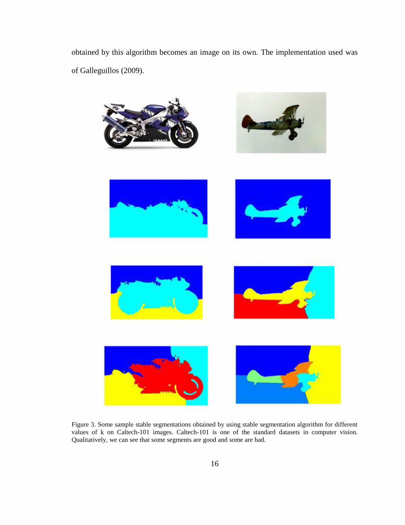
obtained by this algorithm becomes an image on its own. The implementation used was
of Galleguillos (2009).
Figure 3. Some sample stable segmentations obtained by using stable segmentation algorithm for different
values of k on Caltech-101 images. Caltech-101 is one of the standard datasets in computer vision.
Qualitatively, we can see that some segments are good and some are bad.
17
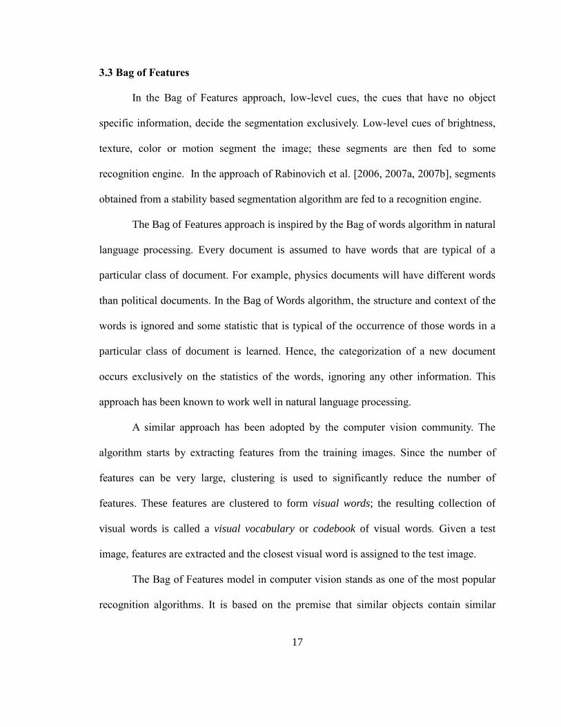
3.3 Bag of Features
In the Bag of Features approach, low-level cues, the cues that have no object
specific information, decide the segmentation exclusively. Low-level cues of brightness,
texture, color or motion segment the image; these segments are then fed to some
recognition engine. In the approach of Rabinovich et al. [2006, 2007a, 2007b], segments
obtained from a stability based segmentation algorithm are fed to a recognition engine.
The Bag of Features approach is inspired by the Bag of words algorithm in natural
language processing. Every document is assumed to have words that are typical of a
particular class of document. For example, physics documents will have different words
than political documents. In the Bag of Words algorithm, the structure and context of the
words is ignored and some statistic that is typical of the occurrence of those words in a
particular class of document is learned. Hence, the categorization of a new document
occurs exclusively on the statistics of the words, ignoring any other information. This
approach has been known to work well in natural language processing.
A similar approach has been adopted by the computer vision community. The
algorithm starts by extracting features from the training images. Since the number of
features can be very large, clustering is used to significantly reduce the number of
features. These features are clustered to form visual words; the resulting collection of
visual words is called a visual vocabulary or codebook of visual words. Given a test
image, features are extracted and the closest visual word is assigned to the test image.
The Bag of Features model in computer vision stands as one of the most popular
recognition algorithms. It is based on the premise that similar objects contain similar

18
parts and the relative location of parts is not very important in recognition. Even with no
spatial information used in recognition, surprisingly, this method works well empirically
Imagine, for example, that the recognition of images of horses is our problem. The Bag of
Features algorithm, when trained on images of horses, will learn statistics of various parts
of horses. That is, the classifier will be trained to recognize feet, mouth, legs, eyes, etc. of
a horse. When the trained classifier receives a new image of a horse, the classifier will
verify that the image contains feet, legs, mouth, eyes, and other parts typical of a horse. If
it finds these parts, it will recognize the image as a horse. There is one downside: the
algorithm does not care about the relative locations of these parts. Hence, a weird
creature that looks like a horse but has eyes located on its foot will be recognized as a
horse too. Nevertheless, statistically, this algorithm works surprisingly well in some
cases.
In the implementation for the purpose of this thesis, the first stage is extraction of
SIFT (Scale Invariant Features Transform) features (Lowe 1999). SIFT features, one of
the most widely used features in computer vision, are known to extract the most
distinctive features from an image. SIFT features are invariant to scale, orientation and
translation, while being partially invariant to illumination and noise. The first stage in the
extraction of SIFT features is scale-space-extrema detection to detect various interest
points in the image. The image is first blurred by applying a Gaussian filter and
subsequently applying a Difference of Gaussian filter at various scales and obtaining
local scale space extrema (interest points) at different points in the image. In the second
stage, the interest points that are low contrast and poorly localized along the edges are

19
discarded. Then for each interest point, the gradient orientation histogram is computed
around the interest point, and the most dominant orientation, that is, the one with highest
magnitude (peak in the histogram), is assigned to the interest point. A 16x16 pixel
window is taken around this point and split into 16 4x4 windows. In each 4x4 window,
the gradient orientation histogram of 8 bins is computed. Finally, an interest point
descriptor is computed by taking the values of all the bins, that is, 4x4x8 = 128. The 128
length vector is normalized to obtain the final descriptor vector.
The next stage of Bag of Features is clustering of features in an unsupervised
manner. Clustering algorithms such as vector-quantization or k-means may be used for
this purpose. From the feature vectors of training images, a dictionary of visual words is
constructed. A “visual word” is a patch in an image, and it is used here in analogy to Bag
of Words models in natural language processing, where we have actual words. The
feature vectors obtained from the training images are clustered to form a visual words
dictionary, where each cluster center represents a visual word. That is, each visual word
is representative of similar feature vectors. For each category, a histogram is constructed
by learning the frequencies of the visual words in that category. The test image is
recognized by measuring its distance from the histograms of all categories in the training
images. The distance measure used could be Manhattan, Euclidean or any other useful
measure.
The performance of the Bag-of-Features algorithm may depend on various design
issues (Hara & Draper 2011). The designer has to make a decision on the choice of
features such as SIFT, SURF (Bay et al. 2008) or any other feature. Another decision is

20
on the choice of clustering algorithm such as k-means, vector-quantization, or any other
similar algorithm. Another decision is about the distance measure such as Manhattan
distance, Euclidean distance, or any other. All of these decisions have the potential to
affect the performance of the algorithm.
In spite of its success, the Bag of Features algorithm is not free from problems
(Hara & Draper 2011). There are several challenges that need to be addressed. There is
no spatial information, hence, the algorithm can be challenging for applications in which
spatial information or relative location of objects is critical. Recognizing relationships
between various objects could be hard with this algorithm. Another challenge is that there
is no semantic meaning attached to the visual codewords. A single visual word may be
composed of features that may have come from different parts of an image.
In the approach used in this thesis, segmentation as a preprocessing step can be
combined with the Bag of Features algorithm. Using the stable segmentation algorithm
described above, each segment becomes a stand-alone image. Each segment is fed to a
Bag of Features recognition engine for classification. For each segment, a label is
obtained. Finally, using some voting criteria, each segment votes for a label and finally
based on the maximum score on the voting criteria, the test image is classified.
3. 4 HMAX
The HMAX model (Serre et al. 2007) accounts for the rapid categorization
abilities of the human brain. In particular, it accounts for object selectivity and
invariance. Recognition of images in a given class is often hard because a new image in
the class can have a wide variety of poses, sizes, colors, textures, clutter and background
21
noise. Hence, it becomes important that we tune for object selectivity and invariance.
HMAX is a hierarchical model with several layers, where the layers alternate between
selectivity and invariance. The HMAX model (Figure 4) is composed of S units and C
units, which are described below.
The Simple Units: Simple (S) Units are used to build object selectivity. S-units
are implemented as Gabor Filters that are tuned to various stimuli at several scales and
orientations. Gabor filters are used for the purpose of the pattern matching between the
input and the prototype represented by that filter. More specifically, S units compare the
input to the stored prototype using a Gabor function, thus obtaining the activation, which
is a measure of the similarity between the input obtained and the prototype. Across all
units, activation map is obtained. Gabor filters have been used to model simple cells in
the visual cortex of the brain.
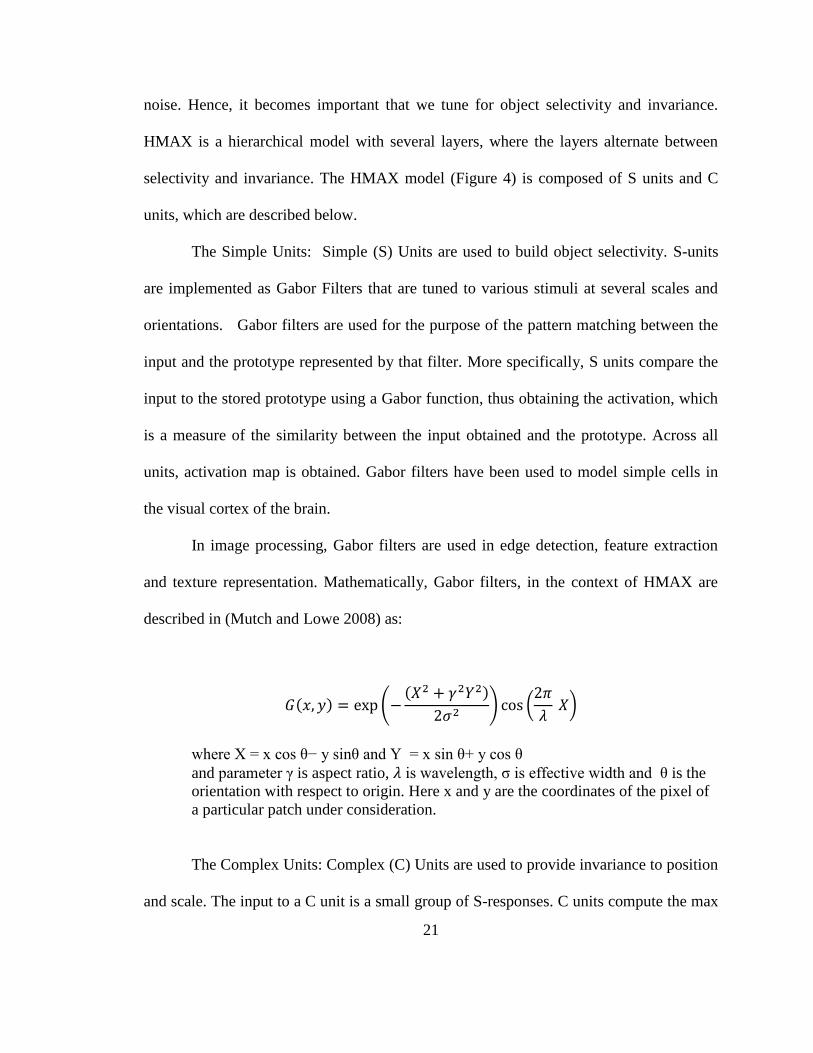
In image processing, Gabor filters are used in edge detection, feature extraction
and texture representation. Mathematically, Gabor filters, in the context of HMAX are
described in (Mutch and Lowe 2008) as:
( ) ( ( )
) (
)
where X = x cos θ− y sinθ and Y = x sin θ+ y cos θ
and parameter γ is aspect ratio, is wavelength, σ is effective width and θ is the
orientation with respect to origin. Here x and y are the coordinates of the pixel of
a particular patch under consideration.
The Complex Units: Complex (C) Units are used to provide invariance to position
and scale. The input to a C unit is a small group of S-responses. C units compute the max

22
function on the responses of S-units that have the same orientation but different scales
and positions.
The HMAX model is built by alternating between S and C units. There are four
layers in most implementations – S1, C1, S2, and C2. S1 units may correspond to edges
in an input image, whereas S2 units correspond to more complex groupings of edges.
Figure 4. The HMAX model (Figure from Isik et al. 2011). S units act as feature detectors and C units are
used to build invariance to position and scale for a particular orientation.

23
3.4 Dataset
The dataset used for the purpose of all the experiments in this thesis is Caltech-
101 (Fei-Fei et al. 2004). Caltech 101 has emerged as one of the standard datasets in the
computer vision community. There are 101 categories in the dataset. Researchers use this
datasets to evaluate and compare their systems. However, the dataset has few
shortcomings. According to the Griffin et al. (2006), the dataset is too easy because
images are left-right aligned and it will saturate performance. Another problem with the
dataset is that images cover most of the area, however, in real world images; this may not
be the case. In addition; there is not enough noise or clutter in the images. We use 35
categories from this datasets. Examples of images from the dataset are shown in Figure 5.

24
Figure 5, Sample Caltech -101 Images

25
Chapter 4
Experimental Methodology and Results
In this chapter we describe the methodology and results of various experiments.
4.1 Experiment 1: Segmentation Preceding Bag of Features
This experiment is to test the hypothesis that segmentation as a preprocessing step
helps recognition. For this experiment, the Bag of Features algorithm was trained as was
described above in Section 3.3. As described in that section, the features are extracted
from the training images using the SIFT algorithm. The features are clustered using a
clustering algorithm called hierarchical k-means. The cluster centers act as visual words.
The frequencies of these visual words are learned for each category and a histogram of
visual word representing each training category is formed. When a test image is fed to
Bag of Features algorithm, its features are extracted using SIFT and a histogram of visual
words is constructed. The test image is assigned the category whose histogram most
closely resembles the histogram of the test image.
The experiment is divided into three parts. In the first part, the training is on
unsegmented images and testing is also on unsegmented images. In the second part, the
training is on manually segmented images and testing is also on manually segmented
images. One may ask why test on manually segmented images? In an ideal world, we
want our original segmentations obtained from the segmentation algorithm to resemble
the manual segmentations. However, as of current state-of-the-art in the segmentation,
this is far from reality. Someday, when progress is made in segmentation driven systems,
we will have ideal segments resembling ground truth segmentations. Hence, we would

26
like to have a crisp idea of how much better we can do with such ideal segmentations. In
addition, this experiment can provide us with an idea of how far the segmentation driven
recognition paradigm is from its original goal.
In the third part, the training is on manually segmented images and testing is on
stable segmentation images. Ideally, here training should also have been on stable
segmentation images. However, most automatic segmentation algorithms of our era yield
horrible segments. To make valid training, I trained on manually segmented images. In many
ways, this experiment is similar to the one conducted by Rabinovich et al. (2007a, b).
The implementation and parameters used for the Bag of Features algorithm were
default in the implementation of Andrea Vedaldi (2010). The dataset used was Caltech-
101. Ten categories were selected from this dataset. Thirty training images and ten test
images were used for each category.
For the stability based segmentation algorithm, the only cues used were brightness
and texture. Each test image is segmented into 54 segments. The number 54 is obtained
by the model order value of parameter k= 10 (Rabinovich et al. 2007). This means that in
the first round, each image is segmented into two segments only. In the second round,
each image is segmented into three segments. In the third round, each image is segmented
into four segments, and so on. Hence, for k=10, we obtain (2+3+4 +5+…+10 = 54) 54
segments. Note that some of the segments will be very small and some of them will be
large, whereas others will be of medium size. Each segment obtained by this method is
made into a standalone image, and is fed to the Bag of Features algorithm for
categorization. Once the category of all segments corresponding to a particular image is
obtained, a final label is assigned to a test image by plurality voting by all the segments.

27
Plurality voting is used in these experiments. This scheme has many advantages. It is
simple and direct. It helps us in capturing insights that will help us in designing a powerful
recognition system. If we are to adopt some segmentation-recognition scheme, where many
segments occur in ensembles, then at least plurality must be attainable by the segments, if
absolute majority is not possible. What is aimed at here is direct insight into segmentation
algorithms of our era. If we are to build and compete with state-of-the-art recognition
systems, we do not seriously want to rely on any segmentation algorithm that will not even
produce segments that are even capable of attaining a plurality vote. The real problem is how
to get a good segmentation when getting a good segmentation depends on getting a good
recognition, and getting a good recognition depends on getting a good segmentation. This
calls for feedback in such systems.
The results for the Experiment 1 are shown in Table 1. The results are described
in the form of confusion matrices. The results for recognition without segmentation are
shown in Table 2. The Y-axis represents the actual category and X-axis represents the
predicted category. For example, in Table 2, of the 10 test images of an ant, 3 are
recognized as an ant, 2 as beaver, 1 as crab, 1 as crayfish and 3 as crocodile_head. The
results of recognition with manual segmentation are shown in Table 3. The results of
recognition with stable segmentation are shown in Table 4. The confusion matrix is
useful in many situations as a visualization tool. It can capture information that other
types of measurement may not be able to capture. For example, Table 2 tells us that 5
crab images were recognized as crocodile_head. This information of inter-category
confusion can be critical information about the behavior of a system.
28
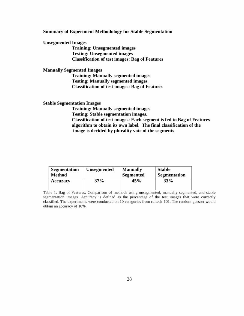
Summary of Experiment Methodology for Stable Segmentation
Unsegmented Images
Training: Unsegmented images
Testing: Unsegmented images
Classification of test images: Bag of Features
Manually Segmented Images
Training: Manually segmented images
Testing: Manually segmented images
Classification of test images: Bag of Features
Stable Segmentation Images
Training: Manually segmented images
Testing: Stable segmentation images.
Classification of test images: Each segment is fed to Bag of Features
algorithm to obtain its own label. The final classification of the
image is decided by plurality vote of the segments
Segmentation
Method
Unsegmented Manually
Segmented
Stable
Segmentation
Accuracy 37% 45% 33%
Table 1: Bag of Features, Comparison of methods using unsegmented, manually segmented, and stable
segmentation images. Accuracy is defined as the percentage of the test images that were correctly
classified. The experiments were conducted on 10 categories from caltech-101. The random guesser would
obtain an accuracy of 10%.

29
Table 2: Confusion Matrix: 10 categories (Bag of Features, No Segmentation). Y-axis is actual category
and x-axis is predicted category. The matrix shows what number of test images of actual category were
classified as the predicted category. The color scale used is Blue-Green-Red, where blue represents the
lowest numbers and red the highest.

30
Table 3: Confusion Matrix: 10 categories (Bag of Features, Manually Segmented). Y-axis is actual
category and x-axis is predicted category. The matrix shows what number of test images of actual category
were classified as the predicted category. The color scale used is Blue-Green-Red, where blue represents
the lowest numbers and red the highest.
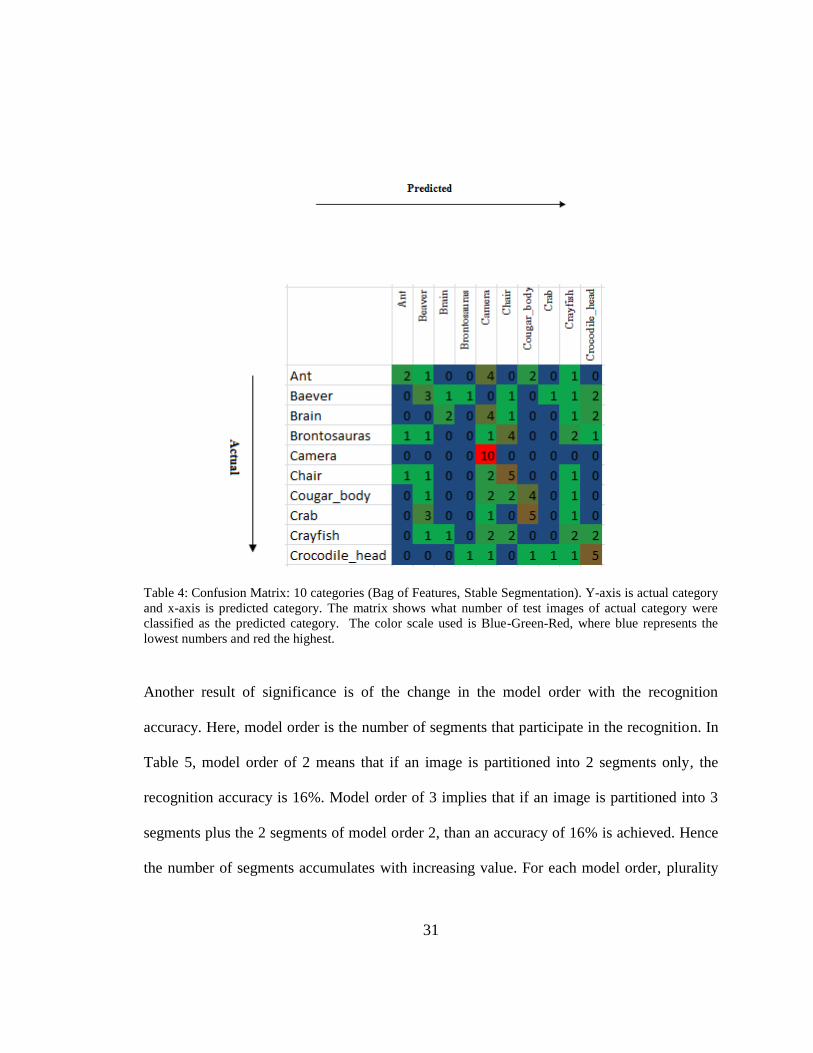
31
Table 4: Confusion Matrix: 10 categories (Bag of Features, Stable Segmentation). Y-axis is actual category
and x-axis is predicted category. The matrix shows what number of test images of actual category were
classified as the predicted category. The color scale used is Blue-Green-Red, where blue represents the
lowest numbers and red the highest.
Another result of significance is of the change in the model order with the recognition
accuracy. Here, model order is the number of segments that participate in the recognition. In
Table 5, model order of 2 means that if an image is partitioned into 2 segments only, the
recognition accuracy is 16%. Model order of 3 implies that if an image is partitioned into 3
segments plus the 2 segments of model order 2, than an accuracy of 16% is achieved. Hence
the number of segments accumulates with increasing value. For each model order, plurality

32
vote is used. In a similar analysis, Rabinovich et al. (2007) had shown that beyond 35
segments, the recognition accuracy is not significantly impacted.
Model Order Number of
Segments
Recognition
accuracy
Random
Guesser
Accuracy
2 2 16% 10%
3 5 16% 10%
4 9 19% 10%
5 14 22% 10%
6 20 18% 10%
7 27 19% 10%
8 35 20% 10%
9 44 19% 10%
10 54 21% 10%
Table 5: Change in recognition accuracy with increasing model order for stable
segmentation test images.
4.2 Experiment 2: Segmentation preceding HMAX
The experiment is exactly similar to the Experiment 1 except with few differences. The
Bag of Features algorithm is replaced by HMAX and multiclass SVM. HMAX acts as a
feature extractor, and multiclass SVM acts a classifier. The HMAX model is initially
trained with training images of all the 10 categories with 1000 prototypes. After training
33
of HMAX is finished, it is switched to the inference mode. In the inference mode, the
feature vectors of all the training images are obtained from HMAX. Separately, the
feature vectors of testing images are obtained from HMAX. The feature vectors of
training images are used to train the multi-class support vector machine (SVM). SVM is a
machine learning algorithm that divides the datapoints in the plane in a way so that the
partition between two classes of data is maximum. This can be used to classify one
category vs another. It is possible to extend such binary class SVMs to multi-class SVMs.
This can be clarified with help of an example. For example, our goal is to classify
categories A vs B vs C vs D. Multi-class SVMs will first classify A vs All. If the category
is not A, then it will classify B vs All, and so on. After the SVM is trained with training
feature vectors obtained from HMAX, it is fed with the feature vectors of the testing
images obtained from HMAX. Each testing image is classified by the SVM. The rest of
the set-up of this experiment is similar to that of Section 4.1. The HMAX implementation
used for the purpose of this thesis was of Mick Thomure (2011). The SVM
implementation was of Thorsten Joachims (2008). The results for Experiment 2 are
shown in Table 6. The results for recognition without segmentation are shown in Table 7.
The results of recognition with manual segmentation are shown in Table 8. The results of
recognition with stable segmentation are shown in Table 9.
Summary of Experiment Methodology for Stable Segmentation
Unsegmented Images
Training: Unsegmented images
Testing: Unsegmented images
Classification of test images: HMAX followed by multi-class SVM.
Manually Segmented Images

34
Training: Manually segmented images
Testing: Manually segmented images
Classification of test images: HMAX followed by multi-class SVM.
Stable Segmentation Images
Training: Manually segmented images
Testing: Stable segmentation images.
Classification of test images: Each segment is fed to the HMAX
algorithm to obtain its feature vector. The feature vector of each
segment is fed to the multi class SVM for labeling. The final
classification of the image is decided by plurality vote of the segments
Segmentation
Method
Unsegmented Manually
Segmented
Stable
Segmentation
Accuracy 29% 21% 9%
Table 6: HMAX, Comparison of methods using unsegmented, manually segmented, and stable
segmentation images. Accuracy is defined as the percentage of the test images that were correctly
classified. The experiments were conducted on 10 categories from caltech-101. A random guesser would
obtain an accuracy of 10%.

35
Table 7: Confusion Matrix: 10 categories (HMAX, No Segmentation). Y-axis is actual category and x-axis
is predicted category. The matrix shows what number of test images of actual category were classified as
the predicted category. The color scale used is Blue-Green-Red, where blue represents the lowest numbers
and red the highest.
36
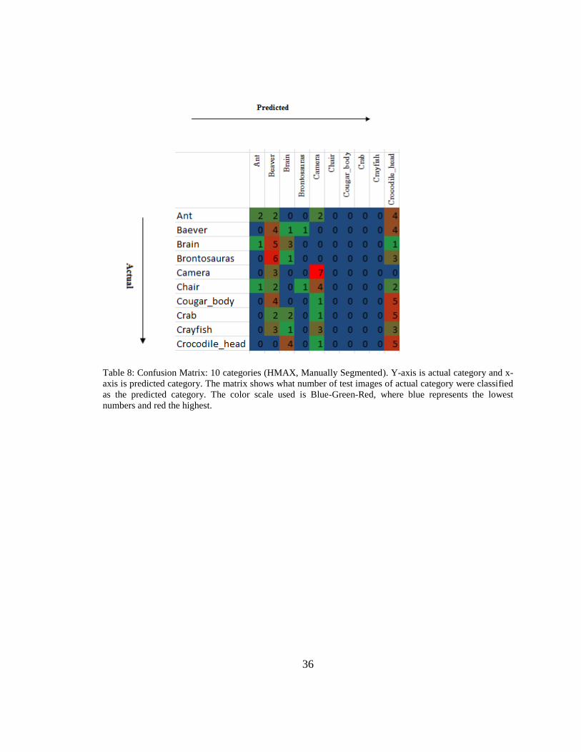
Table 8: Confusion Matrix: 10 categories (HMAX, Manually Segmented). Y-axis is actual category and x-
axis is predicted category. The matrix shows what number of test images of actual category were classified
as the predicted category. The color scale used is Blue-Green-Red, where blue represents the lowest
numbers and red the highest.

37
Table 9: Confusion Matrix: 10 categories (HMAX, Stable Segmentation). Y-axis is actual category and x-
axis is predicted category. The matrix shows what number of test images of actual category were classified
as the predicted category. The color scale used is Blue-Green-Red, where blue represents the lowest
numbers and red the highest.
4.3 Experiment 3: Segmentation preceding Bag of Features (Scaling up)
One of the purposes of this experiment is to explore the scalability of recognition
algorithms. Traditionally, many computer vision algorithms have not had success with
respect to the scalability. If we are to build the state of the art object recognition systems,
we need to have algorithms that scale up on many aspects. Here, we test the scalability of
the recognition algorithms with the number of categories. The experiments are conducted
for a certain number of categories, 10, 20, 30, and 35.
38
Unlike previous experiments, these experiments are conducted by training on
unsegmented images, and testing on both segmented images and unsegmented images.
Since the training is only on unsegmented images, the experiments are bit biased towards
unsegmented images. However, there are two reasons why training on unsegmented
images may be a better idea. First, if our goal is of making large scale general purpose
computer vision system with large number of categories, it may not be pragmatic to
obtain manually segmented images for training. Second, training on automatic segmented
images may not be a good idea as the number of categories becomes very large. The
automatic segmentation algorithms of our era do not yield segments that are good only
few times. Hence, for training, it will only make sense to select segments that contain an
actual object. This extra selection step may not be a feasible option if we are dealing with
very high number of categories. Hence, the case for training on unsegmented images.
The results for Experiment 3 are shown in Tables 10 and 11. The results for recognition
without segmentation are in Table 10 and results for the recognition with segmentation
are in Table 11. The results are described in the form of confusion matrices. The Y-axis
represents the actual category and X-axis represents the predicted category. The results
for recognition without segmentation are shown in Tables 12, 13, 14 and 15. The results
of recognition with segmentation are shown in Tables 16, 17, 18 and 19.
Summary of Experiment Methodology
(Comparison of 10, 20, 30, 35 categories)
Unsegmented Images
Training: Unsegmented images
39
Testing: Unsegmented images
Classification of test images: Bag of Features
Stable Segmentation Images
Training: Unsegmented images
Testing: Stable segmentation images.
Classification of test images: Each segment is fed to Bag of Features
algorithm to obtain its own label. The final classification of the
image is decided by plurality vote of the segments
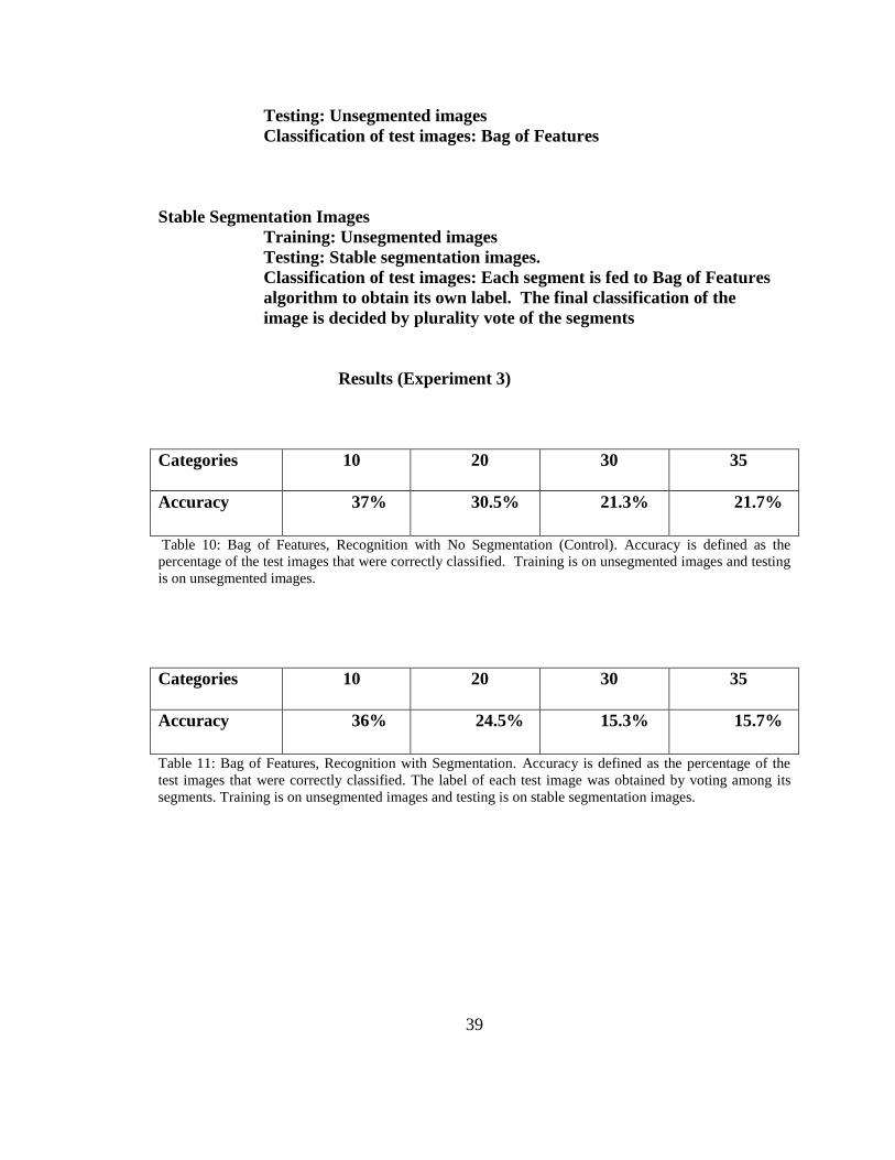
Results (Experiment 3)
Categories 10 20 30 35
Accuracy 37% 30.5% 21.3% 21.7%
Table 10: Bag of Features, Recognition with No Segmentation (Control). Accuracy is defined as the
percentage of the test images that were correctly classified. Training is on unsegmented images and testing
is on unsegmented images.
Categories 10 20 30 35
Accuracy 36% 24.5% 15.3% 15.7%
Table 11: Bag of Features, Recognition with Segmentation. Accuracy is defined as the percentage of the
test images that were correctly classified. The label of each test image was obtained by voting among its
segments. Training is on unsegmented images and testing is on stable segmentation images.

40
Table 12: Confusion Matrix: 10 categories (Bag of Features, No Segmentation). Y-axis is actual category
and x-axis is predicted category. The matrix shows what number of test images of actual category were
classified as the predicted category. The color scale used is Blue-Green-Red, where blue represents the
lowest numbers and red the highest.

41
Table 13: Confusion Matrix: 20 categories (Bag of Features, No Segmentation). Y-axis is actual category
and x-axis is predicted category. The matrix shows what number of test images of actual category were
classified as the predicted category. The color scale used is Blue-Green-Red, where blue represents the
lowest numbers and red the highest.

42
Table 14: Confusion Matrix: 30 categories (Bag of Features, No Segmentation). Y-axis is actual category
and x-axis is predicted category. The matrix shows what number of test images of actual category were
classified as the predicted category. The color scale used is Blue-Green-Red, where blue represents the
lowest numbers and red the highest.

43
Table 15: Confusion Matrix: 35 categories (Bag of Features, No Segmentation). Y-axis is actual category
and x-axis is predicted category. The matrix shows what number of test images of actual category were
classified as the predicted category. The color scale used is Blue-Green-Red, where blue represents the
lowest numbers and red the highest.

44
Table 16: Confusion Matrix: 10 categories (Bag of Features, Segmentation). Y-axis is actual category and
x-axis is predicted category. The matrix shows what number of test images of actual category were
classified as the predicted category. The color scale used is Blue-Green-Red, where blue represents the
lowest numbers and red the highest.

45
Table 17: Confusion Matrix: 20 categories (Bag of Features, Segmentation). Y-axis is actual category and
x-axis is predicted category. The matrix shows what number of test images of actual category were
classified as the predicted category. The color scale used is Blue-Green-Red, where blue represents the
lowest numbers and red the highest.
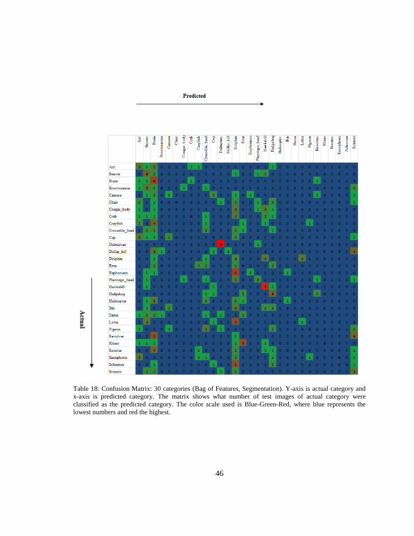
46
Table 18: Confusion Matrix: 30 categories (Bag of Features, Segmentation). Y-axis is actual category and
x-axis is predicted category. The matrix shows what number of test images of actual category were
classified as the predicted category. The color scale used is Blue-Green-Red, where blue represents the
lowest numbers and red the highest.
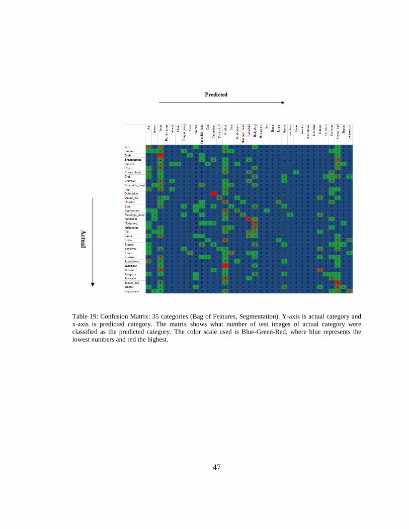
47
Table 19: Confusion Matrix: 35 categories (Bag of Features, Segmentation). Y-axis is actual category and
x-axis is predicted category. The matrix shows what number of test images of actual category were
classified as the predicted category. The color scale used is Blue-Green-Red, where blue represents the
lowest numbers and red the highest.

48
4.4 Experiment 4 : Segmentation preceding HMAX (Scaling up)
The experiment is similar to the experiment 3 except that it is conducted on HMAX
features and multi-class SVM, instead of the Bag of Features. The results for the
Experiment 4 are shown in Tables 20 and 21. The results for recognition without
segmentation are in Table 20 and results for the recognition with segmentation are in
Table 21. The results are described in the form of confusion matrices. The Y-axis
represents the actual category and X-axis represents the predicted category. The results
for recognition without segmentation are shown in Tables 22, 23, 24 and 25. The results
of recognition with segmentation are shown in Tables 26, 27, 28 and 29.
Summary of Experiment Methodology
(Comparison of 10, 20, 30, 35 categories)
Unsegmented Images
Training: Unsegmented images
Testing: Unsegmented images
Classification of test images: HMAX followed by multi-class SVM.
Stable Segmentation Images
Training: Unsegmented images
Testing: Stable segmentation images.
Classification of test images: Each segment is fed to the HMAX
algorithm to obtain its feature vector. The feature vector of each
segment is fed to the multi class SVM for labeling. The final
classification of the image is decided by plurality vote of the segments.
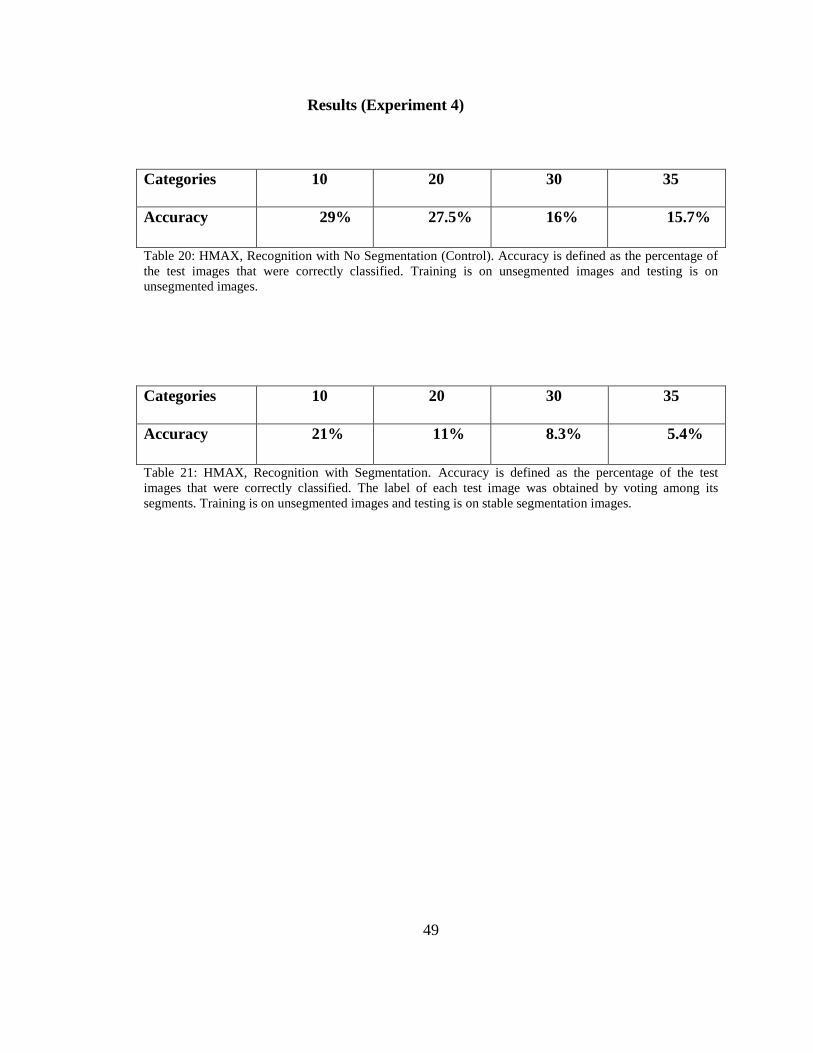
49
Results (Experiment 4)
Categories 10 20 30 35
Accuracy 29% 27.5% 16% 15.7%
Table 20: HMAX, Recognition with No Segmentation (Control). Accuracy is defined as the percentage of
the test images that were correctly classified. Training is on unsegmented images and testing is on
unsegmented images.
Categories 10 20 30 35
Accuracy 21% 11% 8.3% 5.4%
Table 21: HMAX, Recognition with Segmentation. Accuracy is defined as the percentage of the test
images that were correctly classified. The label of each test image was obtained by voting among its
segments. Training is on unsegmented images and testing is on stable segmentation images.

50
Table 22: Confusion Matrix: 10 categories (HMAX, No Segmentation). Y-axis is actual category and x-
axis is predicted category. The matrix shows what number of test images of actual category were classified
as the predicted category. The color scale used is Blue-Green-Red, where blue represents the lowest
numbers and red the highest.

51
Table 23: Confusion Matrix: 20 categories (HMAX, No Segmentation). Y-axis is actual category and x-
axis is predicted category. The matrix shows what number of test images of actual category were classified
as the predicted category. The color scale used is Blue-Green-Red, where blue represents the lowest
numbers and red the highest.

52
Table 24: Confusion Matrix: 30 categories (HMAX, No Segmentation). Y-axis is actual category and x-
axis is predicted category. The matrix shows what number of test images of actual category were classified
as the predicted category. The color scale used is Blue-Green-Red, where blue represents the lowest
numbers and red the highest.
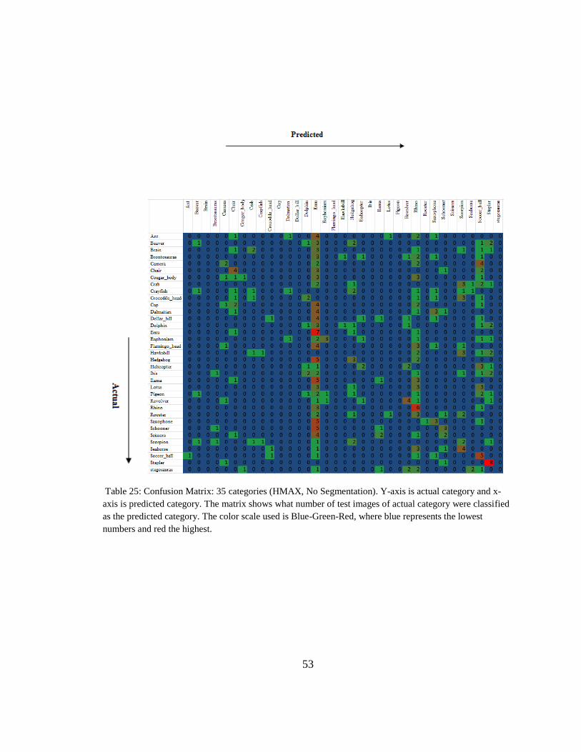
53
Table 25: Confusion Matrix: 35 categories (HMAX, No Segmentation). Y-axis is actual category and x-
axis is predicted category. The matrix shows what number of test images of actual category were classified
as the predicted category. The color scale used is Blue-Green-Red, where blue represents the lowest
numbers and red the highest.

54
Table 26: Confusion Matrix: 10 categories (HMAX, Segmentation). Y-axis is actual category and x-axis is
predicted category. The matrix shows what number of test images of actual category were classified as the
predicted category. The color scale used is Blue-Green-Red, where blue represents the lowest numbers and
red the highest.
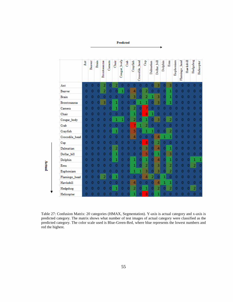
55
Table 27: Confusion Matrix: 20 categories (HMAX, Segmentation). Y-axis is actual category and x-axis is
predicted category. The matrix shows what number of test images of actual category were classified as the
predicted category. The color scale used is Blue-Green-Red, where blue represents the lowest numbers and
red the highest.
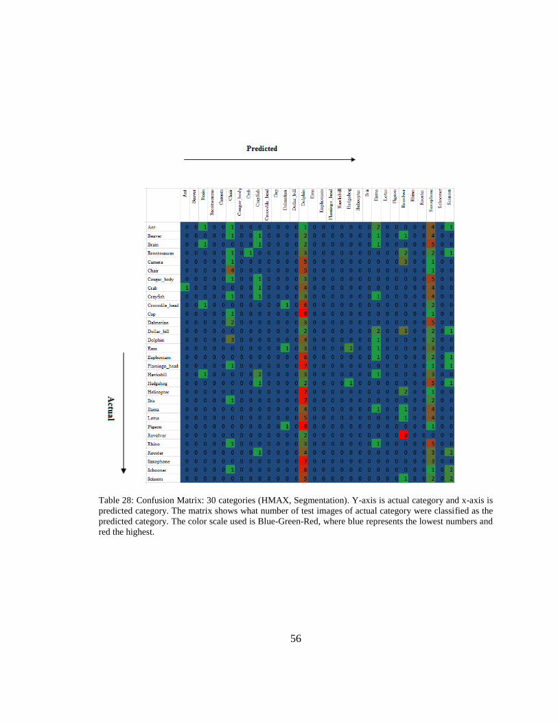
56
Table 28: Confusion Matrix: 30 categories (HMAX, Segmentation). Y-axis is actual category and x-axis is
predicted category. The matrix shows what number of test images of actual category were classified as the
predicted category. The color scale used is Blue-Green-Red, where blue represents the lowest numbers and
red the highest.

57
Table 29: Confusion Matrix: 35 categories (HMAX, Segmentation). Y-axis is actual category and x-axis is
predicted category. The matrix shows what number of test images of actual category were classified as the
predicted category. The color scale used is Blue-Green-Red, where blue represents the lowest numbers and
red the highest.

58
4.5. Results and Discussion
The results obtained on the Bag of Features and HMAX algorithms (Tables 1 –
29) show that in our experiment, automatic segmentation as a preprocessing step does not
increase recognition accuracy. One reason could be that the stable segmentation
algorithm was not able to obtain very high quality segments. Segmentation should in
principle help recognition if we are able to extract spatial information specific to object
and eliminate background noise (Malisiewicz and Efros 2007). However, if in the most of
the segments that we obtained, we are only able to extract partial spatial information and
unable to reduce background noise, then the performance will be adversely affected.
For the training on manually segmented images and testing on the manually segmented
images, in the Bag of Features approach, the manually segmented images outperformed the
unsegmented images. This is expected because the training and testing occurs exclusively on
the actual objects and there is no hindrance from background noise. However, in a weird
result, for the HMAX model, the unsegmented images outperformed the manually segmented
images. This was unexpected. However, there are two explanations. It could be that the
HMAX not only learned the background noise for the unsegmented images, but it learned it
in a way so as to positively affect the recognition accuracy. Another explanation is that
experiments of this nature will always be sensitive to the choice of the data. Maybe on
another data set this will not happen.
What we know of the segmentation algorithms is that each of them have their own
advantages and disadvantages, and the results obtained are highly sensitive to parameters,
type of image and a plethora of other factors (Pantofaru 2008). It may be that we may
not have a single segmentation algorithm that is single-handedly capable of extracting

59
useful spatial information and reducing background noise. In order to circumvent the
problem, some authors have suggested using multiple segmentation algorithms and
combining their results to form high quality segments (Malisiewicz and Efros 2007,
Pantofaru 2008 ).
Another significant question that I intended to answer was of scalability. It is clear
from Tables 9, 10, 19 and 20 that recognition accuracy does not scale well with increase
in number of categories This is not surprising because as we increase the number of
categories, various categories are likely to get confused with one another. For example,
dogs and cats can easily get confused with each other.
Looking at the qualitative results of the stability based segmentation in chapter 3
(Figure 3), we see that some segmentation are very good while others are bad.
Subjectively, the segmentation algorithm does indeed produce good segmentation in
some cases; however, bottom-up segmentation algorithms cannot be relied upon to
always produce useful segmentations.

60
Chapter 5
Conclusion and Future Work
The take home message of this thesis is simple: Automatic segmentation as a
direct preprocessing step to recognition does not seem to improve recognition. However,
does segmentation still have something to contribute to recognition? Using multiple or
blended segments (Malisiewicz and Efros, 2007, Pantofaru 2008, Russell et al. 2006, Tu
et al. 2005) may yield high quality segments that may actually increase recognition
accuracy. This popular approach that is gaining in prominence makes the use of multiple
segmentations obtained from multiple segmentation algorithms. The specific information
captured by each algorithm is different from another. Hence, we need to find a way to
leverage the advantages of each type of algorithm in a single setting. If we use multiple
segmentation algorithms, then each algorithm can correct and compensate for the others’
weaknesses, and thus possibly obtain a better segmentation. Significant progress has been
made in this direction by Malisiewicz and Efros (2007) Russell et al. (2006), Tu et al.
(2005), and Pantofaru (2008).
Another reason that segmentation might not produce good results is because of
intra-category confusion. We know that segmentation is as yet an unsolved problem and
determining high quality segments is not always possible with current segmentation
algorithms. Hence, most algorithms will not be able to correctly segment-out a given
object for the requisite application. This can possibly lead to intra-category confusion.
For example, imagine a segment that contains a dog's body parts except for the head.
Imagine another segment that contains a cat's body parts except the head. Since body

61
parts of both dogs and cats are very similar, there is a chance for confusion by a
recognition engine. One of the goals of segmentation is to successfully capture spatial
information, which if correctly captured, could possibly lead to successful recognition.
But even minute failure to capture spatial information might significantly curtail any
benefits that we might accrue for segmentation.
Incorporation of feedback is the most natural next step in segmentation-driven
recognition models. Psychologists and neuroscientists have long known the role of
feedback in the human recognition processes. By incorporating feedback, segments will
have a shot at self-correction and self-modification based on the feedback. The feedback
coming from the recognition system can improve the quality of the segmentation. Thus,
by forming an interactive process of top-down and bottom-up segmentation, recognition
accuracy can be increased. There are obvious challenges for such a system. Such a
system will have to address time and space complexity issues. Moreover, we do not yet
know how to algorithmically create such a system, though there is a great deal of current
research on the subject.

62
References
Bay, H., Ess, A., Tuytelaars T., & Gool, L. V. (2008). SURF: Speeded Up Robust
Features. Computer Vision and Image Understanding, 110, 3, 346--359.
Borenstein, E., & Ullman, S. (2002). Class-specific, top-down segmentation. In
Proceedings of European Conference on Computer Vision, 109–124.
Fei-Fei, L., Fergus, R. & Perona, P. (2004). Learning generative visual models from few
training examples: an incremental Bayesian approach tested on 101 object categories.
IEEE Conference on Computer Vision and Pattern Recognition, Workshop on
Generative-Model Based Vision.
Forsyth, D. A. & Ponce, J. (2003). Computer Vision: A Modern Approach. Prentice Hall.
Galleguillos, C. (2009). Personal Communication.
Griffin, H. A. & Perona, P. (2006). Retrieved in 6/2011 from
http://lear.inrialpes.fr/SicilyWorkshop/
Hara, S. O. & Draper, B.A. (2011). Introduction to the bag of features paradigm for
image classification and retrieval. Computing Research Repository, arXiv:1101.3354v1.
Isik, L., Leibo, J.Z., Mutch, J. Lee, S.W. & Poggio, T. (2011) A hierarchical model of
peripheral vision. MIT-CSAIL-TR-2011-031/CBCL-300, Massachusetts Institute of
Technology, Cambridge, MA.
Joachims, T. (2008). http://svmlight.joachims.org/svm_multiclass.html
Lowe, David G. (1999). Object recognition from local scale-invariant features.
Proceedings of the International Conference on Computer Vision. 2 1150–1157.
Malik, J. & Shi, J. B. (2000). Normalized Cuts and Image Segmentation. IEEE
Transactions on Pattern Analysis and Machine Intelligence, 22(8), 888-905.
Malisiewicz, T., & Efros, A., (2007). Improving Spatial Support for Objects via Multiple
Segmentations. Robotics Institute. Paper 280. http://repository.cmu.edu/robotics/280
Mutch, J. & Lowe, D. G. (2008). Object class recognition and localization using sparse
features with limited receptive fields. International Journal of Computer Vision (IJCV),
80(1), 45-57.
Pantofaru, C. (2008). Studies in Using Image Segmentation to Improve Object
Recognition. CMU-RI-TR-08-23, Robotics Institute, Carnegie Mellon University.

63
Pantofaru, C., Dork´o, G., Schmid, C., & Hebert, M. (2006). Combining regions and
patches for object class localization. The Beyond Patches Workshop in conjunction with
the IEEE conference on Computer Vision and Pattern Recognition, 23 – 30.
Pantofaru, C., Schmid, C., & Hebert, M. (2008). Object Recognition by Integrating
Multiple Image Segmentations Proc. European Conference on Computer Vision (ECCV),
October, 2008.
Rabinovich, A., Belongie, S.J., Lange, T. & Buhmann, J.M. (2006). Model Order
Selection and Cue Combination for Image Segmentation. IEEE Conference on Computer
Vision and Pattern Recognition, 1130-1137.
Rabinovich, A., Vedaldi, A. & Belongie, S. (2007). Does image segmentation improve
object categorization? University of California San Diego Technical Report cs2007-0908.
Rabinovich, A., Vedaldi, A., Galleguillos, C., Wiewiora, E. & Belongie, S. (2007).
Objects in Context. IEEE International Conference of Computer Vision (ICCV), 1-8.
Russell, B., Efros, A., Sivic, J., Freeman, W., & Zisserman, A. (2006). Using multiple
segmentations to discover objects and their extent in image collections. IEEE Conference
on Computer Vision and Pattern Recognition.
Serre, T., Kreiman, G., Kouh, M., Cadieu, C., Knoblich, U., & Poggio, T. (2007). A
quantitative theory of immediate visual recognition. Progress in Brain Research,
Computational Neuroscience: Theoretical Insights into Brain Function, 165, 33–56.
Shotton, J., Winn, J., Rother, C, & Criminisi, A. (2009). Textonboost for image
understanding: Multi-class object recognition and segmentation by jointly modeling
texture, layout, and context. Int. Journal of Computer Vision (IJCV), Springer Verlag.
Thomure, M. (2011). Personal Communication.
Tu, Z., Chen, Z., Yuille, A.L., & Zhu, S.C. (2005). Image parsing: Unifying
segmentation, detection, and recognition. In Proceedings of Toward Category-Level
Object Recognition, 45-576.
Unnikrishnan, R., Pantofaru, C., & Hebert, M. (2007). Toward objective evaluation of
image segmentation algorithms. IEEE Transactions on Pattern Analysis and Machine
Intelligence, 29 ( 6), 929-944.
Vecera, S. P., & Farah, M. J. (1997). Is visual image segmentation a bottom-up or an
interactive process? Perception & Psychophysics, 59, 1280-1296.

64
Vedaldi, A. (2010) Bag of Features. Retrieved in 2010 from
http://www.vlfeat.org/~vedaldi/code/bag/bag.html