The linear/nonlinear model s*f 1. The spike-triggered average.
46
he linear/nonlinear model s*f 1
-
Upload
sam-chilcote -
Category
Documents
-
view
214 -
download
1
Transcript of The linear/nonlinear model s*f 1. The spike-triggered average.
The linear/nonlinear model
s*f1

The spike-triggered average

More generally, one can conceive of the action of the neuron or neural system as selecting a low dimensional subset of its inputs.
Start with a very high dimensional description (eg. an image or a time-varying waveform)
and pick out a small set of relevant dimensions.
s(t)
s1s2 s3
s1
s2
s3
s4 s5 s.. s.. s.. sn S(t) = (S1,S2,S3,…,Sn)
Dimensionality reduction
P(response | stimulus) P(response | s1, s2, .., sn)
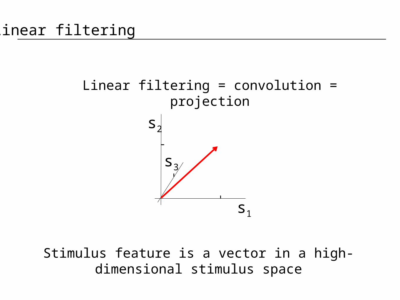
Linear filtering
Linear filtering = convolution = projection
s1
s2
s3
Stimulus feature is a vector in a high-dimensional stimulus space

How to find the components of this model
s*f1

The input/output function is:
which can be derived from data using Bayes’ rule:
Determining the nonlinear input/output function
Tuning curve: P(spike|s) = P(s|spike) P(spike) / P(s)
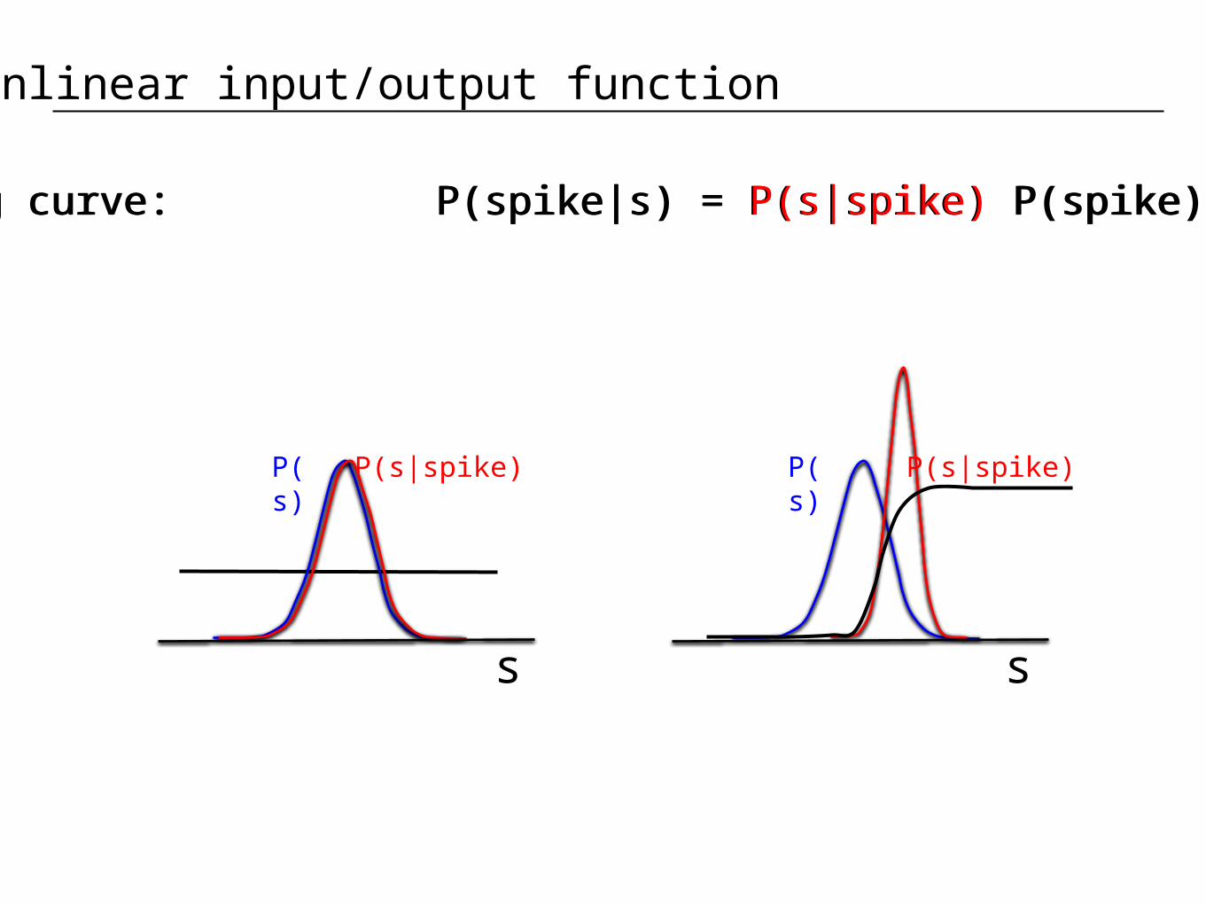
Nonlinear input/output function
Tuning curve: P(spike|s) = P(s|spike) P(spike) / P(s)
s
P(s|spike) P(s)
s
P(s|spike) P(s)

Models with multiple features
Linear filters & nonlinearity: r(t) = g(f1*s, f2*s, …, fn*s)

Spike-triggeredaverage
Gaussian priorstimulus distribution
Spike-conditional distribution
covariance
Determining linear features from white noise

The covariance matrix is
Properties:
• The number of eigenvalues significantly different from zero is the number of relevant stimulus features
• The corresponding eigenvectors are the relevant features (or span the relevant subspace)
Stimulus prior
Bialek et al., 1988; Brenner et al., 2000; Bialek and de Ruyter, 2005
Identifying multiple features
Spike-triggered stimulus correlation
Spike-triggeredaverage
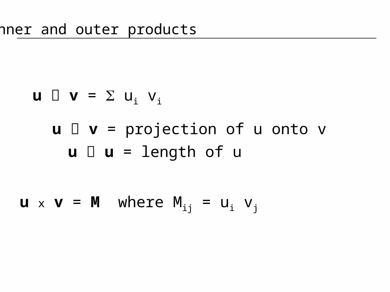
Inner and outer products
u v = S ui vi
u v = projection of u onto v
u u = length of u
u x v = M where Mij = ui vj

Eigenvalues and eigenvectors
M u = l u

Singular value decomposition
m
n
=
xx
M
U S V
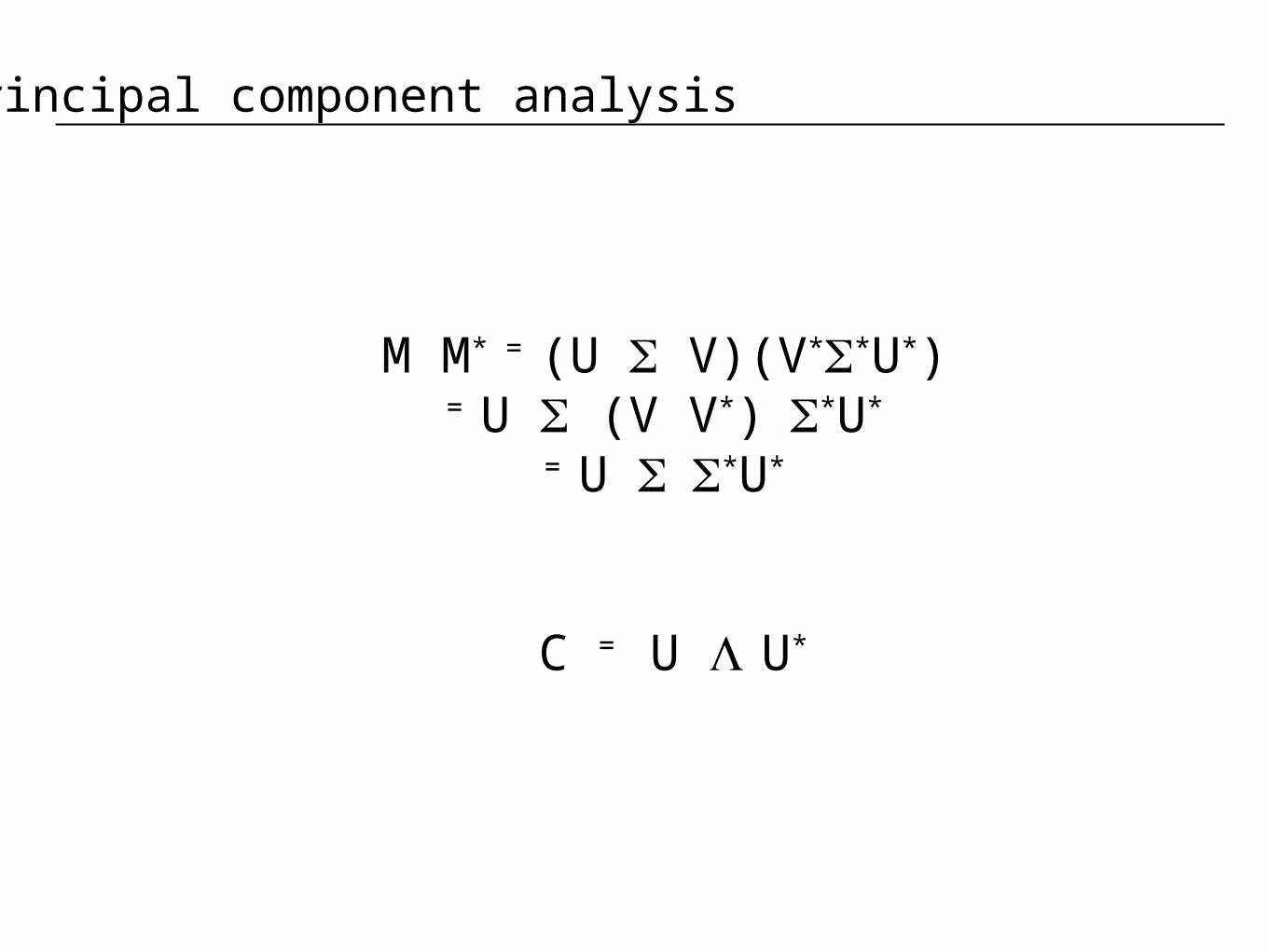
Principal component analysis
M M* = (U S V)(V*S*U*)= U S (V V*) S*U*
= U S S*U*
C = U L U*

The covariance matrix is
Properties:
• The number of eigenvalues significantly different from zero is the number of relevant stimulus features
• The corresponding eigenvectors are the relevant features (or span the relevant subspace)
Stimulus prior
Bialek et al., 1988; Brenner et al., 2000; Bialek and de Ruyter, 2005
Identifying multiple features
Spike-triggered stimulus correlation
Spike-triggeredaverage

Let’s develop some intuition for how this works: a filter-and-fire threshold-crossing model with AHP
Keat, Reinagel, Reid and Meister, Predicting every spike. Neuron (2001)
• Spiking is controlled by a single filter, f(t)• Spikes happen generally on an upward threshold crossing of
the filtered stimulus expect 2 relevant features, the filter f(t) and its time derivative f’(t)
A toy example: a filter-and-fire model

6
4
2
0
-2P
roje
ctio
n o
nto
Mo
de
26420-2
Projection onto Mode 1
-0.6
-0.4
-0.2
0.0
0.2
0.4
0.6
Sp
ike
-Tri
gg
ere
d A
vera
ge
-0.5 -0.4 -0.3 -0.2 -0.1 0.0Time before Spike (s)
STAf(t)
f'(t)
6
4
2
0
-2P
roje
ctio
n o
nto
Mo
de
2
6420-2
Projection onto Mode 1
6
4
2
0
-2P
roje
ctio
n o
nto
Mo
de
2
6420-2
Projection onto Mode 1
-1.0
-0.5
0.0
0.5
1.0
Eig
en
valu
e
50403020100Mode Index
Covariance analysis of a filter-and-fire model

Example: rat somatosensory (barrel) cortex Ras Petersen and Mathew Diamond, SISSA
0 200 400 600 800 1000
-400
-200
0
200
400
Time (ms)
Stim
ulat
or
posi
tion
(m
)
Record from single units in barrel cortex
Some real data
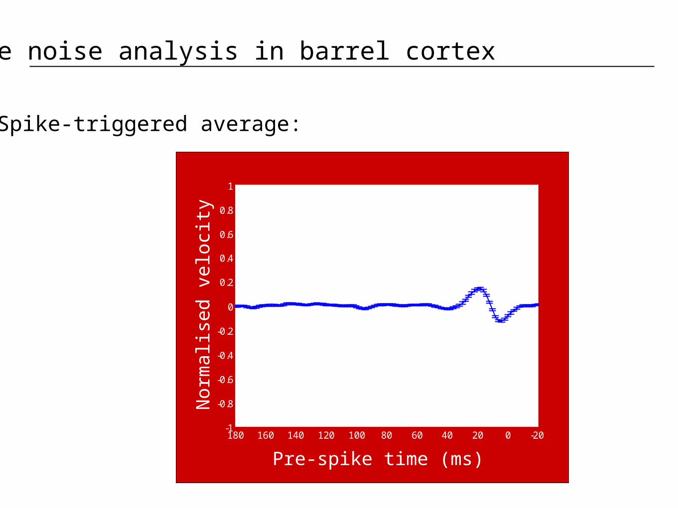
Spike-triggered average:
-20020406080100120140160180-1
-0.8
-0.6
-0.4
-0.2
0
0.2
0.4
0.6
0.8
1
Pre-spike time (ms)
Norm
alis
ed v
elo
city
White noise analysis in barrel cortex

Is the neuron simply not very responsive to a white noise stimulus?
White noise analysis in barrel cortex

Prior Spike-triggered
Difference
Covariance matrices from barrel cortical neurons

0 20 40 60 80 100-1
0
1
2
3
4
Feature number
No
rmal
ised
vel
oci
ty2
050100150-0.4
-0.3
-0.2
-0.1
0
0.1
0.2
0.3
0.4
Pre-spike time (ms)
Ve
loci
ty
Eigenspectrum
Leading modes
Eigenspectrum from barrel cortical neurons

-3 -2 -1 0 1 2 30
2
4
6
8
10
Normalised "acceleration"
No
rmal
ised
firi
ng r
ate
-3 -2 -1 0 1 2 30
2
4
6
8
10
12
Normalised "velocity"
No
rmal
ised
firi
ng r
ate
-2 0 2
-3
-2
-1
0
1
2
3
"acceleration"
"vel
oci
ty"
0
2
4
6
8
10
0 1 2 30
2
4
6
8
10
"vel"2+"acc"2
No
rmal
ised
firi
ng r
ate
Input/outputrelations wrt
first two filters,alone:
and in quadrature:
Input/output relations from barrel cortical neurons

050100150-0.2
-0.1
0
0.1
0.2
0.3
0.4
0.5
Pre-spike time (ms)
Velo
city (
arb
itra
ry u
nits)
050100150-0.3
-0.2
-0.1
0
0.1
0.2
0.3
0.4
Pre-spike time (ms)Velo
city
(arb
itra
ry u
nit
s)
How about the other modes?
Next pair with +ve eigenvaluesPair with -ve eigenvalues
Less significant eigenmodes from barrel cortical neurons

0 0.5 1 1.5 2 2.5 30
0.5
1
1.5
"Energy"N
orm
alis
ed f
iring
rat
e
-3 -2 -1 0 1 2-3
-2
-1
0
1
2
Filter 100
Filt
er 1
01
0.2
0.4
0.6
0.8
1
1.2
1.4
Firing rate decreases with increasing projection: suppressive modes
Input/output relations for negative pair
Negative eigenmode pair

-0.4
-0.2
0.0
0.2
0.4
Sp
ike
-Tri
gg
ere
d A
vera
ge
-0.5 -0.4 -0.3 -0.2 -0.1 0.0Time before Spike (s)
STA
-0.4
-0.2
0.0
0.2
0.4
Sp
ike
-Tri
gg
ere
d A
vera
ge
-0.5 -0.4 -0.3 -0.2 -0.1 0.0Time before Spike (s)
STA Mode 1
-0.4
-0.2
0.0
0.2
0.4
Sp
ike
-Tri
gg
ere
d A
vera
ge
-0.5 -0.4 -0.3 -0.2 -0.1 0.0Time before Spike (s)
STA Mode 1 Mode 2
-1.0
-0.5
0.0
0.5
1.0
Eig
en
valu
e
100806040200Mode Index
-6
-4
-2
0
2
4
6
Pro
ject
ion
on
to M
od
e 2
-4 -2 0 2 4
Projection onto Mode 1
Salamander retinal ganglion cells perform a variety of computations
Michael Berry

-0.4
-0.2
0.0
0.2
0.4
Sp
ike
-Tri
gg
ere
d A
vera
ge
-0.8 -0.6 -0.4 -0.2 0.0Time before Spike (s)
STA
-6
-4
-2
0
2
4
6
Pro
ject
ion
on
to M
od
e 2
-4 -2 0 2 4
Projection onto Mode 1
-1.0
-0.5
0.0
0.5
Eig
en
valu
e
100806040200Mode Index
-0.4
-0.2
0.0
0.2
0.4
Sp
ike
-Tri
gg
ere
d A
vera
ge
-0.8 -0.6 -0.4 -0.2 0.0Time before Spike (s)
STA Mode 1
-0.4
-0.2
0.0
0.2
0.4
Sp
ike
-Tri
gg
ere
d A
vera
ge
-0.8 -0.6 -0.4 -0.2 0.0Time before Spike (s)
STA Mode 1 Mode 2
-0.4
-0.2
0.0
0.2
0.4
Sp
ike
-Tri
gg
ere
d A
vera
ge
-0.8 -0.6 -0.4 -0.2 0.0Time before Spike (s)
STA Mode 1 Mode 2 Mode 3
Almost filter-and-fire-like

1.0
0.5
0.0
-0.5
Eig
en
valu
e
100806040200Mode Index
-0.4
-0.2
0.0
0.2
0.4
Sp
ike
-Tri
gg
ere
d A
vera
ge
-0.8 -0.6 -0.4 -0.2 0.0Time before Spike (s)
STA
-0.4
-0.2
0.0
0.2
0.4
Sp
ike
-Tri
gg
ere
d A
vera
ge
-0.8 -0.6 -0.4 -0.2 0.0Time before Spike (s)
STA Mode 1
-0.4
-0.2
0.0
0.2
0.4
Sp
ike
-Tri
gg
ere
d A
vera
ge
-0.8 -0.6 -0.4 -0.2 0.0Time before Spike (s)
STA Mode 1 Mode 2
-0.4
-0.2
0.0
0.2
0.4
Sp
ike
-Tri
gg
ere
d A
vera
ge
-0.8 -0.6 -0.4 -0.2 0.0Time before Spike (s)
STA Mode 1 Mode 2 Mode 3
-6
-4
-2
0
2
4
6
Pro
ject
ion
on
to M
od
e 2
-6 -4 -2 0 2 4 6
Projection onto Mode 1
Not a threshold-crossing neuron

-0.4
-0.2
0.0
0.2
0.4
Sp
ike
-Tri
gg
ere
d A
vera
ge
-0.5 -0.4 -0.3 -0.2 -0.1 0.0Time before Spike (s)
STA
-0.4
-0.2
0.0
0.2
0.4
Sp
ike
-Tri
gg
ere
d A
vera
ge
-0.5 -0.4 -0.3 -0.2 -0.1 0.0Time before Spike (s)
STA Mode 1
-0.4
-0.2
0.0
0.2
0.4
Sp
ike
-Tri
gg
ere
d A
vera
ge
-0.5 -0.4 -0.3 -0.2 -0.1 0.0Time before Spike (s)
STA Mode 1 Mode 2
-0.4
-0.2
0.0
0.2
0.4
Sp
ike
-Tri
gg
ere
d A
vera
ge
-0.5 -0.4 -0.3 -0.2 -0.1 0.0Time before Spike (s)
STA Mode 1 Mode 2 Mode 3
0.9
0.6
0.3
0.0
-0.3
Eig
en
valu
e
100806040200
Mode Index
2.0
1.5
-6
-4
-2
0
2
4
6
Pro
ject
ion
on
to M
od
e 2
-6 -4 -2 0 2 4 6
Projection onto Mode 1
Complex cell like

-0.6
-0.3
0.0
0.3
Eig
en
valu
e
100806040200
Mode Index
2.5
2.0
-0.4
-0.2
0.0
0.2
0.4
Sp
ike
-Tri
gg
ere
d A
vera
ge
-0.6 -0.4 -0.2 0.0Time before Spike (s)
STA
-0.4
-0.2
0.0
0.2
0.4
Sp
ike
-Tri
gg
ere
d A
vera
ge
-0.6 -0.4 -0.2 0.0Time before Spike (s)
STA Mode 1
-0.4
-0.2
0.0
0.2
0.4
Sp
ike
-Tri
gg
ere
d A
vera
ge
-0.6 -0.4 -0.2 0.0Time before Spike (s)
STA Mode 1 Mode 2 Mode 3
-4
-3
-2
-1
0
1
2
3
4
Pro
ject
ion
on
to M
od
e 2
-6 -4 -2 0 2 4 6
Projection onto Mode 1
Bimodal: two separate features are encoded as either/or

Complex cells in V1
Rust et al., Neuron 2005
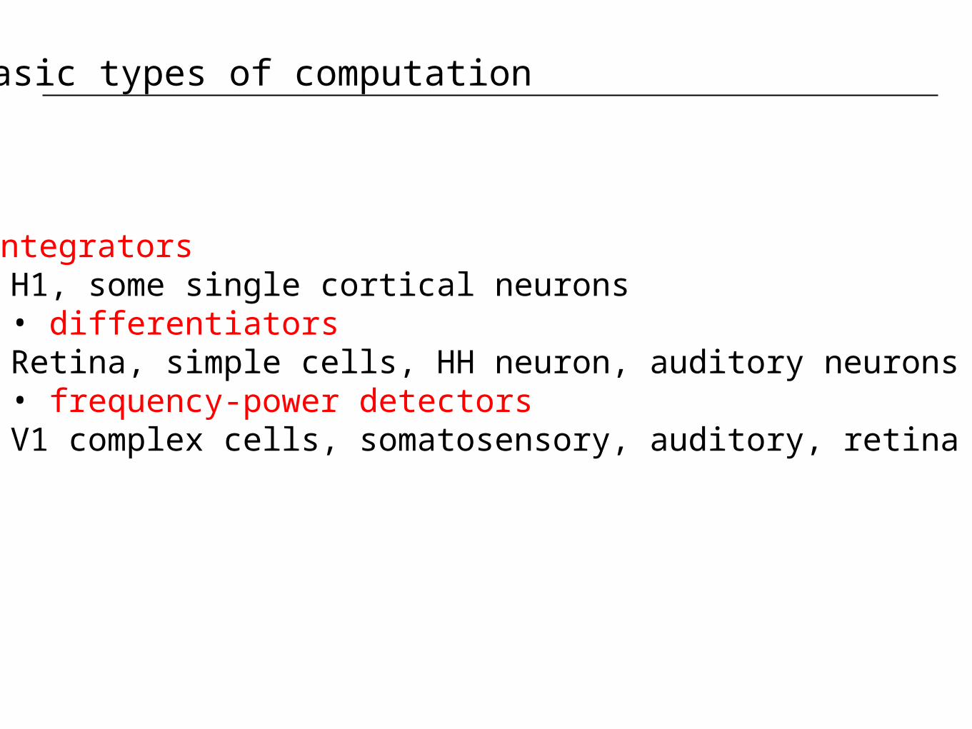
• integrators H1, some single cortical neurons• differentiators Retina, simple cells, HH neuron, auditory neurons• frequency-power detectors V1 complex cells, somatosensory, auditory, retina
Basic types of computation
When have you done a good job?
• When the tuning curve over your variable is interesting.
• How to quantify interesting?

Tuning curve: P(spike|s) = P(s|spike) P(spike) / P(s)
Goodness measure: DKL(P(s|spike) | P(s))
When have you done a good job?
Tuning curve: P(spike|s) = P(s|spike) P(spike) / P(s)
s
Boring: spikes unrelated to stimulus
P(s|spike) P(s)
s
Interesting: spikes are selective
P(s|spike) P(s)

Maximally informative dimensions
Choose filter in order to maximize DKL between spike-conditional and prior distributions
Equivalent to maximizing mutual information between stimulus and spike
Sharpee, Rust and Bialek, Neural Computation, 2004
Does not depend on white noise inputs
Likely to be most appropriatefor deriving models fromnatural stimuli
s = I*f
P(s|spike) P(s)
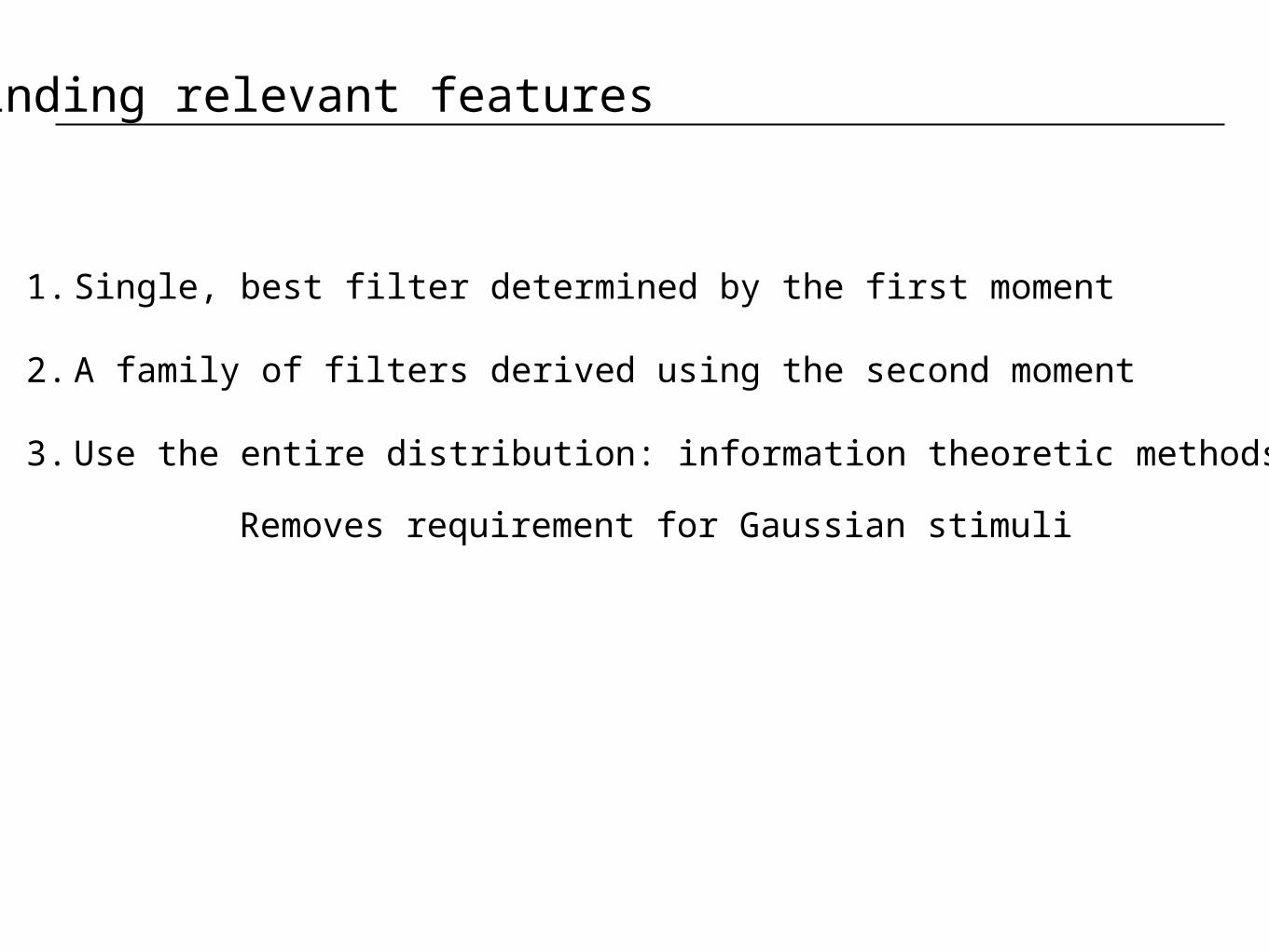
1. Single, best filter determined by the first moment
2. A family of filters derived using the second moment
3. Use the entire distribution: information theoretic methods
Removes requirement for Gaussian stimuli
Finding relevant features

Less basic coding models
Linear filters & nonlinearity: r(t) = g(f1*s, f2*s, …, fn*s)
…shortcomings?

Less basic coding models
GLM: r(t) = g(f1*s + f2*r)
Pillow et al., Nature 2008; Truccolo, .., Brown, J. Neurophysiol. 2005

Less basic coding models
GLM: r(t) = g(f*s + h*r)
…shortcomings?

Less basic coding models
GLM: r(t) = g(f1*s + h1*r1 + h2*r2 +…)
…shortcomings?

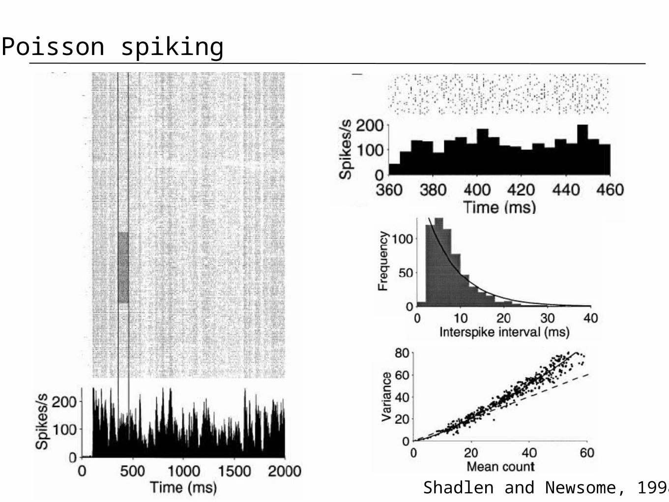
Poisson spiking
Poisson spiking
Shadlen and Newsome, 1998

Poisson spiking
Properties:
Distribution: PT[k] = (rT)k exp(-rT)/k!
Mean: <x> = rT
Variance: Var(x) = rT
Interval distribution: P(T) = r exp(-rT)
Fano factor: F = 1

Fano factor Data fit to: variance = A meanB
A
B
Area MT
Poisson spiking in the brain

How good is the Poisson model? ISI analysis
ISI Distribution from an area MT Neuron
ISI distribution generated from a Poisson model with a Gaussian refractory period
Poisson spiking in the brain

Hodgkin-Huxley neuron driven by noise