The Limited Information Maximum Likelihood...
33
The Limited Information Maximum Likelihood Estimator as an Angle ∗ T. W. Anderson † Naoto Kunitomo ‡ and Yukitoshi Matsushita § March 27, 2009 Abstract When an econometric structural equation includes two endogenous variables and their coefficients are normalized so that their sum of squares is 1, it is natural to express them as the sine and cosine of an angle. The Limited Information Maximum Likelihood (LIML) estimator of this angle when the error covariance matrix is known has constant variance. Of all estimators with constant variance the LIML estimator minimizes the variance. Competing estimators, such as the Two-Stage Least Squares estimator, has much larger variance for some values of the parameter. The effect of weak instruments is studied. Key Words Structural equation, linear functional relationship, natural normalization, angle LIML, finite sample properties. ∗ This is the version AKM09-3-27-2. † Department of Statistics and Department of Economics, Stanford University ‡ Graduate School of Economics, University of Tokyo § Graduate School of Economics, University of Tokyo 1
-
Upload
nguyenthuy -
Category
Documents
-
view
217 -
download
0
Transcript of The Limited Information Maximum Likelihood...

The Limited Information MaximumLikelihood Estimator as an Angle ∗
T. W. Anderson †
Naoto Kunitomo ‡
and
Yukitoshi Matsushita §
March 27, 2009
Abstract
When an econometric structural equation includes two endogenous variables andtheir coefficients are normalized so that their sum of squares is 1, it is natural toexpress them as the sine and cosine of an angle. The Limited Information MaximumLikelihood (LIML) estimator of this angle when the error covariance matrix is knownhas constant variance. Of all estimators with constant variance the LIML estimatorminimizes the variance. Competing estimators, such as the Two-Stage Least Squaresestimator, has much larger variance for some values of the parameter. The effect ofweak instruments is studied.
Key Words
Structural equation, linear functional relationship, natural normalization, angleLIML, finite sample properties.
∗This is the version AKM09-3-27-2.†Department of Statistics and Department of Economics, Stanford University‡Graduate School of Economics, University of Tokyo§Graduate School of Economics, University of Tokyo
1
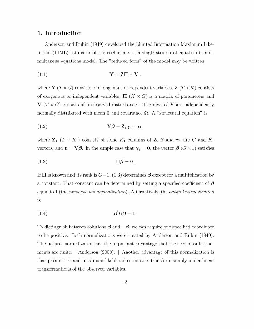
1. Introduction
Anderson and Rubin (1949) developed the Limited Information Maximum Like-
lihood (LIML) estimator of the coefficients of a single structural equation in a si-
multaneus equations model. The ”reduced form” of the model may be written
Y = ZΠ + V ,(1.1)
where Y (T ×G) consists of endogenous or dependent variables, Z (T ×K) consists
of exogenous or independent variables, Π (K × G) is a matrix of parameters and
V (T × G) consists of unobserved disturbances. The rows of V are independently
normally distributed with mean 0 and covariance Ω. A ”structural equation” is
Yβ = Z1γ1 + u ,(1.2)
where Z1 (T × K1) consists of some K1 columns of Z, β and γ1 are G and K1
vectors, and u = Vβ. In the simple case that γ1 = 0, the vector β (G× 1) satisfies
Πβ = 0 .(1.3)
If Π is known and its rank is G−1, (1.3) determines β except for a multiplication by
a constant. That constant can be determined by setting a specified coefficient of β
equal to 1 (the conventional normalization). Alternatively, the natural normalization
is
β′Ωβ = 1 .(1.4)
To distinguish between solutions β and −β, we can require one specified coordinate
to be positive. Both normalizations were treated by Anderson and Rubin (1949).
The natural normalization has the important advantage that the second-order mo-
ments are finite. [ Anderson (2008). ] Another advantage of this normalization is
that parameters and maximum likelihood estimators transform simply under linear
transformations of the observed variables.
2
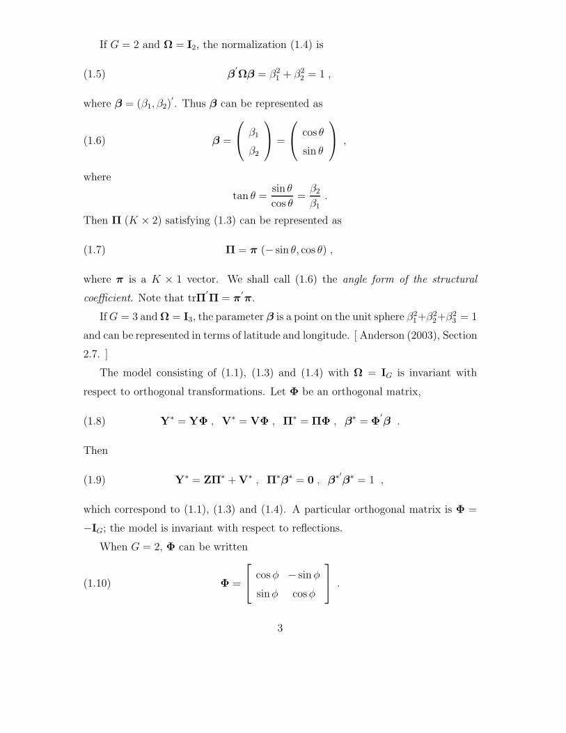
If G = 2 and Ω = I2, the normalization (1.4) is
β′Ωβ = β2
1 + β22 = 1 ,(1.5)
where β = (β1, β2)′. Thus β can be represented as
β =
⎛⎝ β1
β2
⎞⎠ =
⎛⎝ cos θ
sin θ
⎞⎠ ,(1.6)
where
tan θ =sin θ
cos θ=
β2
β1
.
Then Π (K × 2) satisfying (1.3) can be represented as
Π = π (− sin θ, cos θ) ,(1.7)
where π is a K × 1 vector. We shall call (1.6) the angle form of the structural
coefficient. Note that trΠ′Π = π
′π.
If G = 3 and Ω = I3, the parameter β is a point on the unit sphere β21+β2
2+β23 = 1
and can be represented in terms of latitude and longitude. [ Anderson (2003), Section
2.7. ]
The model consisting of (1.1), (1.3) and (1.4) with Ω = IG is invariant with
respect to orthogonal transformations. Let Φ be an orthogonal matrix,
Y∗ = YΦ , V∗ = VΦ , Π∗ = ΠΦ , β∗ = Φ′β .(1.8)
Then
Y∗ = ZΠ∗ + V∗ , Π∗β∗ = 0 , β∗′β∗ = 1 ,(1.9)
which correspond to (1.1), (1.3) and (1.4). A particular orthogonal matrix is Φ =
−IG; the model is invariant with respect to reflections.
When G = 2, Φ can be written
Φ =
⎡⎣ cos φ − sin φ
sinφ cosφ
⎤⎦ .(1.10)
3

Then
β∗ = Φ′β =
⎡⎣ cosφ sin φ
− sin φ cosφ
⎤⎦
⎡⎣ cos θ
sin θ
⎤⎦ =
⎡⎣ cos(θ − φ)
sin(θ − φ)
⎤⎦ .(1.11)
A rotation of β in the angular form corresponds to a translation of the angle.
If γ1 = 0 and β1 = 1, the structural equation (1.2) is
y1 = −β2y2 + u ,(1.12)
where Y = (y1,y2) and the angle representation is written as
β2 =sin θ
cos θ= tan θ .(1.13)
On the other hand, if γ1 = 0 and β2 = 1, the structural equation (1.2) is written as
y2 = −β1y1 + u′,(1.14)
and the angle representation is
β1 = cot θ =1
tan θ.(1.15)
In this paper we consider the distribution of the angle LIML estimator, which is
invariant to orthogonal transformations, in a systematic way. On the other hand, the
Two-Stage Least Squares (TSLS) estimator and the Generalized Method of Moments
(GMM) estimator for coefficients, which have been often used in recent econometric
studies, depend crucially on the particular normalization chosen in advance. (See
Anderson and Sawa (1977).) This issue is related to the properties of alternative
estimators and the optimality of estimation in structural equations. Some aspects
of the related problems have been discussed by Anderson, Stein and Zaman (1985),
Hiller (1990) and Chamberlain (2007). In particular we shall investigate the behavior
of the adaptation of the LIML estimator to the case of Ω known, that is, the LIMLK
estimator, and compare it to the TSLS estimator in some detail. This simple case
makes clearer some properties of these estimators.
A typical and simple application of simultaneous equations has been the econo-
metric analysis of the demand-supply relation in markets. In such case we could take
4

the log-quantity as y1 and the log-price as y2, and then we can estimate the price
elasticity of the demand, for instance. The LIML estimate of the price elasticity
is invariant whether we estimate it by using the demand function or the inverse-
demand function as economists often do their empirical analysis interchangeably in
real applications.
2. Inference when G = 2 and Ω = I2
The maximum likelihood estimator of Π when Π is unrestricted is
P = A−1Z′Y , A = Z
′Z .(2.1)
Let
G = P′AP , G =
1
TG = P
′AP , A =
1
TA .(2.2)
Note that P is a sufficient statistic for Π, which is the only parameter when Ω is
known.
Let d1 and d2 (d1 < d2) be the roots of
0 = |G − dI2| = d2 − (g11 + g22)d + g11g22 − g212 ,(2.3)
where G = (gij). The smaller root of (2.3) is
d1 =1
2
[g11 + g22 −
√(g11 − g22)2 + 4g2
12
].(2.4)
The LIMLK estimator b of β with the natural normalization satisfies 1 = b′b =
b21 + b2
2 and
0 =(G − d1I2
)b(2.5)
=
⎡⎣ (g11 − d1)b1 + g12b2
g21b1 + (g22 − d1)b2
⎤⎦ .
The second component of (2.5) leads to the LIMLK estimator of θ as the solution
of
tan θ =b2
b1
= − 2g21
g22 − g11 +√
(g22 − g11)2 + 4g212
.(2.6)
5

Note that the denominator of (2.6) is positive.
The Two-Stage Least Squares (TSLS) estimator is defined by the second com-
ponent of (2.5) with d1 replaced by 0. The equation is
g21b1 + g22b2 = 0 .(2.7)
The TSLS estimator of θ is defined by
tan θTS =b2
b1
= − g21
g22
.(2.8)
Note that the sign of tan θTS is the same as the sign of tan θ and
| tan θTS| < | tan θ| .(2.9)
In a sense tan θTS is biased towards 0.
A transformation (1.8) effects a transformation of P to
P∗ = PΦ(2.10)
and b, the solution to (2.5), to
Φ′b = b∗ =
⎡⎣ b∗1
b∗2
⎤⎦ .(2.11)
Then θ defined by (2.5) is transformed to θ∗ defined by
b∗2b∗1
= tan θ∗ .(2.12)
Thus θ∗ = θ − φ.
Theorem 1 : Let θ∗ = θ − φ, d1 be the smaller root of (2.3), b the vector
satisfying (2.5) and θ the solution to (2.6). Let d∗1, b∗ and θ∗ be the root, vector
and the angle for the model transformed by (1.8). Then θ − θ = θ∗ − θ∗.
Note that the distribution of θ − θ is symmetric. In this sense θ is an unbiased
estimator of θ. Theorem 1 implies that the distribution of θ− θ is independent of θ.
6

The variance of the maximum likelihood estimator θ is invariant under orthogonal
transformations.
Consider the transformation
Z+ = ZM , Π+ = M−1Π ,(2.13)
where M is nonsingular, then (1.3) is transformed to
Π+β = 0 .(2.14)
Furthermore, A transforms to A+ = M′AM, P transforms to P+ = M−1P and
P′AP = P+′
A+P+.
Corollary 1 : The LIMLK estimator with the natural normalization is invariant
with respect to the transformation (2.13).
Anderson (2008) has shown that the normalization (1.4) implies that E(b′b) <
∞.
Note that the LIMLK estimator of θ or of β2/β1 is unaffected by a scale trnsfor-
mation; that is, the LIMLK estimator of β2/β1 based on G is the same as the LIMLK
estimator based on cG, where c > 0. Similarly the TSLS estimator is unaffected by
a scale transformation.
3. A Canonical Form
Make the transformation (2.13) so that A+ = IK , that is, M′AM = IK . Let
P+ = M−1P = Q and
M−1P = Q , M−1π = η ,M−1Π = η(− sin θ, cos θ) .(3.1)
In the case of G = 2, the model is
Q = η (− sin θ, cos θ) + W ,(3.2)
7

where
W = M−1A−1Z′V = M
′Z
′V ,(3.3)
and the rows of W are independently distributed according to N(0, I2). Note that
G = P′AP = Q
′Q and
Π′AΠ = η
′η
⎡⎣ − sin θ
cos θ
⎤⎦ (− sin θ, cos θ) .(3.4)
The ”canonical form” is closely related to the classical ”errors-in-variables”
model, also known as a ”linear functional relationship” in statistics. Suppose Q =
(qki), k = 1, · · · ,K; i = 1, 2, E(qki − μki) = 0, E(qki − μki)2 = σ2, E(qk1 − μk1)(qk2 −
μk2) = 0. The pairs (μk1, μk2) are considered to lie on a straight line
μk2 = α + ρμk1 , k = 1, · · · ,K.(3.5)
When α = 0 and ρ = tan θ, this model corresponds to (3.2). Adcock (1878) recom-
mended estimating α and ρ by minimizing
K∑k=1
[(qk1 − μk1)
2 + (qk2 − μk2)2]
(3.6)
subject to (3.5). This solution agrees with the LIMLK estimator. Anderson (1976)
pointed out this relationship between the LIMLK estimator and the maximum likeli-
hood estimator of the slope in the linear functional relationships. See also Anderson
(1982) and Anderson and Sawa (1982).
In the linear functional relationship in terms of (3.5) it is natural to describe the
line by the angle it makes with the first coordinate axis and the intercept on one of
the coordinate axis. The estimator of this angle was studied by Anderson (1976).
4. Admissibility of the LIMLK estimator
Anderson, Stein and Zaman (1985) have considered the best invariant estimator
8

of a direction. The model corresponds to (3.2) with η′η = λ2. The loss function is
L(β, λ2; β) = 1 − (β′β)2(4.1)
= 1 −⎡⎣(cos θ, sin θ)
⎛⎝ cos θ
sin θ
⎞⎠
⎤⎦
2
= sin2(θ − θ) .
Lemma 1 : Let β∗ = Φ′β and β
∗= Φ
′β as in (1.11). Then
L(β∗, λ2; β∗) = L(β, λ2; β) .(4.2)
Let β− = −β and β−
= −β. Then
L(β−, λ2; β−) = L(β, λ2; β) .(4.3)
Proof : The left-hand side of (4.3) is 1 minus
β∗′β∗
= β′ΦΦ
′β = β
′β .(4.4)
Q.E.D.
The loss function L(β, λ2; β) is invariant under rotations and reflections.
Lemma 2 : Under the transformation (1.8), E(θ − θ)2 is invariant.
Anderson, Stein and Zaman (1985) showed that of all invariant procedures the
LIMLK estimator has minimum loss.
By using the Taylor series expansion of sin x = x − x3/6 + x5/120 − · · · , we
obtain an approximation
E sin2(θ − θ) ∼ E(θ − θ)2 − 1
3E(θ − θ)4 +
2
45E(θ − θ)6 + · · · .(4.5)
5. Empirical Distributions
9

We write (3.2) as
qk1 = −ηk sin θ + wk1 , qk2 = ηk cos θ + wk2 ,(5.1)
where the random variables {wkj} , k = 1, · · · ,K, j = 1, 2, are N(0, 1). Define
λ2 = η′η , α
′= (− sin θ, cos θ) .(5.2)
The matrix Q′Q has a noncentral Wishart distribution with covariance matrix I2,
noncentrality matrix η′ηαα
′and K degrees of freedom [Anderson and Girshick
(1944)]. The exact distributions of b and θ have been given by Anderson and Sawa
(1982), but they are very complicated.
The asymptotic expansions of the distributions of the angle LIMLK and TSLS
estimators (λ → ∞, K fixed) are
P (λ(θLIMLK − θ) ≤ ξ) = Φ(ξ)− 1
2λ2[(K − 1)ξ +
1
3ξ3]φ(ξ) + O(λ−4),(5.3)
and
P (λ(θTS − θ) ≤ ξ) = Φ(ξ) +K − 1
λtan θφ(ξ)(5.4)
− 1
2λ2[{(K − 1)2 tan2 θ − (K − 1)}ξ +
1
3ξ3]φ(ξ) + O(λ−3),
respectively (Anderson (1976)).
For symmetric intervals, the expansions are
P (λ(θLIMLK − θ) ≤ ξ) − P (λ(θLIMLK − θ) ≤ −ξ)(5.5)
= Φ(ξ) − Φ(−ξ) − 1
λ2
[(K − 1)ξ +
1
3ξ3
]φ(ξ) + O(λ−4),
and
P (λ(θTS − θ) ≤ ξ) − P (λ(θTS − θ) ≤ −ξ)(5.6)
= Φ(ξ) − Φ(−ξ) − 1
λ2
[{(K − 1)2 tan2 θ − (K − 1)
}ξ +
1
3ξ3
]φ(ξ) + O(λ−3) .
Then
P (λ|θLIMLK − θ| ≤ ξ) − P (λ|θTS − θ| ≤ ξ)(5.7)
=1
λ2(K − 1)
[(K − 1) tan2 θ − 2
]φ(ξ) + O(λ−3) .
10
The LIMLK estimator dominates the TSLS estimator unless tan2 θ ≤ 2/(K − 1).
The expansion (5.3) corresponds to an approximate density
φ(ξ)− 1
2λ2
[K − 1 − (K − 2)ξ2 − 1
3ξ4
]φ(ξ)(5.8)
and the variance of (5.8) is
1 − 1
2λ2
[(K − 1) − 3(K − 2) − 15
3
]= 1 +
K
λ2.(5.9)
Then the approximate variance of θLIMLK − θ is
1
λ2+
K
λ4.(5.10)
The expansion (5.4) corresponds to an approximate density
φ(ξ)− K − 1
λtan θξφ(ξ)(5.11)
− 1
2λ2
[(K − 1)2 tan2 θ − (K − 1) +
{−(K − 1)2 tan2 θ + K}
ξ2 − 1
3ξ4
]φ(ξ) .
The integral of (5.11) times ξ2, which is an approximate MSE of λ(θTS − θ), is
1 +1
λ2
[(K − 1)2 tan2 θ − K + 2
].(5.12)
Note that the approximate MSE increases with θ from 1 − (K − 2)/λ2 to ∞. The
approximate MSE of the TSLS estimator is less than the approximate MSE of the
LIMLK estimator if tan2 θ < 2/(K − 1). For K = 3 the inequality is tan θ < 1 (θ <
π/4) and for K = 30 tan θ <√
2/29 (= 0.069). We give some numerical values of
the appromimate MSE in Tables 1 and 2.
The empirical distributions of the (standardized) angle LIMLK and TSLS esti-
mators, −π2
< θ − θ < π2,
P (λ(θ − θ) ≤ ξ),(5.13)
and the asymptotic expansions (5.3) and (5.4) are compared. See Figures 1 to 18 in
the appendix.For each K, λ and θ, 10,000 data sets were obtained. The estimate of the loss
E[sin2(θ − θ)], E[sin2(θ − θ)] = 110000
∑10000j=1 sin2(θj − θ), and the estimate of the
11

Table 1: Approximate MSE of θ − θ
K = 3
λ2 = 100 λ2 = 50 λ2 = 10
θ LIMLK TSLS LIMLK TSLS LIMLK TSLS
0.4π 0.0103 0.0212 0.13
0.2π 0.0103 0.0101 0.0212 0.0204 0.13 0.1111
0 0.0103 0.0099 0.0212 0.0196 0.13 0.0900
Table 2: Approximate MSE of θ − θ
K = 30
λ2 = 100 λ2 = 50 λ2 = 10
θ LIMLK TSLS LIMLK LIMLK
0.4π 0.013 0.032 0.4
0.2π 0.013 0.032 0.4
0 0.013 0.0072 0.032 0.4
Table 3: Esin2(θ − θ)
K = 3
λ2 = 100 λ2 = 50 λ2 = 10
θ LIMLK TSLS LIMLK TSLS LIMLK TSLS
0.4π 0.0102 0.0175 0.0206 0.0619 0.1269 0.3580
0.2π 0.0102 0.0100 0.0210 0.0202 0.1276 0.1039
0 0.0102 0.0098 0.0205 0.0187 0.1273 0.0798
12

Table 4: Esin2(θ − θ)
K = 30
λ2 = 100 λ2 = 50 λ2 = 10
θ LIMLK TSLS LIMLK TSLS LIMLK TSLS
0.4π 0.0130 0.3503 0.0340 0.5752 0.2760 0.8184
0.2π 0.0130 0.0353 0.0338 0.0806 0.2693 0.2456
0 0.0131 0.0077 0.0335 0.0123 0.2701 0.0244
Table 5: E(θ − θ)2
K = 3
λ2 = 100 λ2 = 50 λ2 = 10
θ LIMLK TSLS LIMLK TSLS LIMLK TSLS
0.4π 0.0103 0.0191 0.0210 0.0762 0.1561 0.5382
0.2π 0.0103 0.0101 0.0214 0.0206 0.1584 0.1224
0 0.0103 0.0099 0.0209 0.0191 0.1572 0.0879
Table 6: E(θ − θ)2
K = 30
λ2 = 100 λ2 = 50 λ2 = 10
θ LIMLK TSLS LIMLK TSLS LIMLK TSLS
0.4π 0.0131 0.4214 0.0356 0.8024 0.4055 1.3909
0.2π 0.0136 0.0361 0.0355 0.0844 0.3902 0.2797
0 0.0133 0.0077 0.0354 0.0125 0.3927 0.0250
13

MSE, 110000
∑10000j=1 (θj − θ)2 were calculated. (See Tables 3 to 6.) The empirical cdf
of an estimator is within 0.02 of the true cdf everywhere with probability more than0.99 on the basis of 10,000 replications by using the Kolmogorov-Smirnov statistic.(See Anderson, Kunitomo and Sawa (1982).)
Comments on the empirical distributions of the LIMLK and TSLS esti-
mators when Ω = I2
1. The empirical values of E[sin2(θ − θ)] and E[(θ − θ)2] for the LIMLK estimator
are invariant with respect to θ for each pair of value of λ and K.
2. The empirical values of E[sin2(θ − θ)] and E[(θ − θ)2] for the TSLS estimator at
each pair of values of λ and K increase with θ from a value less than the measure
at θ = 0 to a value considerably greater than the measure at θ = π/2.
3. Since λ(θLIMLK − θ) has a limiting distribution N(0, 1), the variance of θLIMLK
is approximately 1/λ2. In Tables 5 and 6 the empirical variance of the LIMLK esti-
mator is approximately .01 for λ2 = 100 and .02 for λ2 = 50, but is approximately
.16 for λ2 = 10 and K = 3 and .39 for λ2 = 10 and K = 30. For smaller values of
λ2 the approximation 1/λ2 underestimates the variance.
4. The estimate of E[sin2(θ − θ)] is less than the estimate of E[(θ − θ)2] for λ2 = 10
for every θ and K.
5. At λ2 = 100 and λ2 = 50, the distributions of λ(θ − θ) for the LIMLK estimator
are almost exactly N(0, 1).
6. More General Models
6.1 Arbitrary Variance
If the covariance matrix Ω of the disturbances is σ2I2, the noncentrality param-
14

eter is
λ2 =η
′η
σ2.(6.1)
6.2 Arbitrary Intercept
If γ1 �= 0, we partition Z and Π as
Z = (Z1,Z2) , Π =
⎡⎣ Π1
Π2
⎤⎦ ,(6.2)
where Z1 has K1 columns, Z2 has K2 columns (K1 + K2 = K), Π1 has K1 rows,
and Π2 has K2 rows. Then (1.3) is replaced by
⎡⎣ Π1
Π2
⎤⎦ β =
⎡⎣ γ1
0
⎤⎦ .(6.3)
The second part of (6.3) determines β. Let
A22.1 = A22 − A21A−111 A12 , Z
′2.1 = Z
′2 − A21A
−111 Z
′1 .(6.4)
Then
P2 = A−122.1Z
′2.1Y , G = P
′2A22.1P2 .(6.5)
Then the proceeding analysis applies with Π replaced by Π2.
6.3 General Ω
When Ω is known, the LIMLK estimator of β in the natural parameterization
is defined by
(P
′AP − d1 Ω
)b = 0 , b
′Ωb = 1 ,(6.6)
where d1 is the smallest root of
|P′AP − d Ω| = 0 .(6.7)
15

This case can be reduced to the special case of Ω = IG. Write Ω = Φ′ΔΦ, where
Δ is diagonal and Φ is orthogonal and
Ω1/2 = Φ′Δ1/2Φ(6.8)
is the symmetric square root of Ω. Then (6.6) can be written
(P
′AP − d1 (Ω1/2)2
)b = 0 , b
′(Ω1/2)2b = 1 ,(6.9)
which leads to
(P∗′AP∗ − d1 IG
)b∗ = 0 , b∗′b∗ = 1 ,(6.10)
where
P∗ = PΩ−1/2 , Ω1/2b∗ = b .(6.11)
Let
Π∗ = ΠΩ−1/2 , β∗ = Ω1/2β .(6.12)
Then
Π∗β∗ = 0 , β∗′β∗ = 1 .(6.13)
When G = 2,
β∗ =
⎡⎣ cos θ∗
sin θ∗
⎤⎦ , b∗ =
⎡⎣ cos θ∗
sin θ∗
⎤⎦ .(6.14)
The case of Ω known, not necessarily IG, can be reduced to the case of Ω = IG.
7. LIML when Ω is unknown
This model consisting of (1.1), (1.3) and (1.4) is invariant with respect to non-
singular transformations
Y∗ = YC , V∗ = VC , Ω∗ = C′ΩC, Π∗ = ΠC , β∗ = C−1β ;(7.1)
16

that is
Π∗β∗ = 0, β∗′Ω∗β∗ = 1 .(7.2)
When Ω is unknown, let b be the solution of
(G − d1 H)b = 0, b′Hb = 1,(7.3)
and d1 is the smallest root of
|G − d H| = 0,(7.4)
G = (1/T )G and
H = Y′Y − G, H =
1
TH .(7.5)
Then Ω = (1/T )H + d1(1/T )Hbb′(1/T )H and the LIML estimator of β is
β =1√
1 + d1
b .(7.6)
The transformation (7.1) effects the transformation
P∗ = PC , G∗ = C′GC, H∗ = C
′HC, b∗ = C−1b .(7.7)
The transformed estimator of β satisfies
(G∗ − d1H∗)b∗ = 0, b∗′Hb∗ = 1,(7.8)
In this sense the LIML estimator is invariant with respect to nonsingular linear
transformations.
Let Ω1/2 be the symmetric square root of Ω defined by (6.8). Then Π∗ = ΠΩ−1/2
and β∗ = Ω1/2β satisfy (7.2). When G = 2, we can define
β∗ =
⎡⎣ cos θ∗
sin θ∗
⎤⎦ .(7.9)
Let H1/2 be the symmetric square root of H. Then β∗
= H1/2b satisfies
(H−1/2GH−1/2 − d1 I2)β∗
= 0, β∗′β
∗= 1,(7.10)
17

Define θ∗ by
β∗
=
⎡⎣ cos θ∗
sin θ∗
⎤⎦ .(7.11)
Then θ∗ is the maximum likelihood estimator of θ∗.
As T → ∞, Gp→ Π
′(limT→∞ A)Π, H
p→ Ω, d1p→ 0, b
p→ β and βp→ β.
Hence θ∗ p→ θ∗. However, θ
∗ − θ∗ does not have an invariant distribution for
fixed T because the transformation C that carries β to β∗ is not the same as the
transformation C that carries β to β∗.
8. The Noncentral Wishart Distribution
The (central) Wishart distribution of G with the covariance matrix Ω = I2,
Π = O, and K degrees of freedom is
w2(G|I2,K) =|G|(K−3)/2e−
12tr G
2Kπ1/2Γ[K/2]Γ[(K − 1)/2)].(8.1)
The matrix G can be represented as
G = ORO′
,(8.2)
where R is diagonal with diagonal elements r1 and r2 (0 ≤ r1 ≤ r2 < ∞) and O is
orthogonal. The orthogonal matrix O can be written as
O =
⎡⎣ cos t − sin t
sin t cos t
⎤⎦ .(8.3)
The diagonal elements of R are the roots of |G − rI2| = 0. The Jacobian of the
transformation (8.2) of (g11, g12, g22) to (r1, r2, t) is r2 − r1. (See Chapter 13 of
Anderson (2003).) Also tr(G) = r1 + r2 and |G| = r1r2. The density of r1, r2 and t
is
(r1r2)(K−3)/2e−
12(r1+r2)(r2 − r1)
2Kπ1/2Γ[K/2]Γ[(K − 1)/2)].(8.4)
18

Note that (r1, r2) and t are independent. The distribution of O is the same as the
distribution of OΦ, where Φ is the orthogonal matrix defined by (1.10). It follows
that the distribution of t is the same as the distribution of t − φ; the distribution
of t is uniform on (0, 2π). Since we identify t with −t and hence with 2π − t, the
density of t is 1/π on the interval [−π/2, π/2].
Let
G = Q′Q = (ηα
′+ W)
′(ηα
′+ W) .(8.5)
The density of G [Anderson and Girshick (1944)] is
w2(G|η′ηαα
′, I2,K) =
e−12η′η− 1
2tr G|G|K−3
2
2Kπ1/2Γ(K−12
)
∞∑j=0
(α′Gα η
′η)j
22jj! Γ(K2
+ j),(8.6)
where α′= (− sin θ, cos θ) and
α′Gα = g11 sin2 θ − 2g12 sin θ cos θ + g22 cos2 θ .(8.7)
Note that for η′η = 0, (8.6) is the same as (8.1).
Let G = ORO′as in (8.2). Then
α′Gα = α
′ORO
′α(8.8)
and
O′α =
⎡⎣ cos t sin t
− sin t cos t
⎤⎦
⎡⎣ − sin θ
cos θ
⎤⎦ =
⎡⎣ sin(t − θ)
cos(t − θ)
⎤⎦ ,(8.9)
which is α with t replaced by t − θ. Thus
α′Gα = [sin(t − θ), cos(t − θ)]
⎡⎣ r1 0
0 r2
⎤⎦
⎡⎣ sin(t − θ)
cos(t − θ)
⎤⎦(8.10)
= r1 sin2(t − θ) + r2 cos2(t − θ)
= r1 + (r2 − r1) cos2(t − θ) .
19

The density of r1, r2 and t is
f(r1, r2, t|η′η, θ) =
1
2Kπ1/2Γ(K−12
)e−
12η′η− 1
2(r1+r2)(r1r2)
12(K−3)(r2 − r1)(8.11)
×∞∑
j=0
[r1 sin2(t − θ) + r2 cos2(t − θ)]j(η′η)j
22jj! Γ(j + 12K)
=1
2Kπ1/2Γ(K−12
)e−
12λ2− 1
2(r1+r2)(r1r2)
12(K−3)(r2 − r1)
×∞∑
j=0
[r1 + (r2 − r1) cos2(t − θ)]j(λ2)j
22jj! Γ(j + 12K)
.
Then (8.4) in r1, r2, t is f(r1, r2, t|0, 0). The marginal density of t is obtained by
integrating (8.11) over 0 ≤ r1 ≤ r2 < ∞. Note that (8.11) is a convergent series.
For each r1 and r2 (r1 ≤ r2) (8.10) is a decreasing function of t − θ for 0 ≤t − θ ≤ π/2; its maximum occurs at t − θ = 0. If (8.11) is considered as the
likelihood function of the parameter θ, it is maximized at θ = t (defined in (8.4)).
Thus θ = t is the maximum likelihood estimator of θ.
In the general case with G > 2, it has been known that the distribution of the
LIML estimator for coefficients has a complicated form. The finite sample properties
of the LIML estimator for coefficients have been explored by Phillips (1984, 1985),
for instance.
9. Weak Instruments
Consider the case of LIML when Ω = IG. The LIML estimator of β when
normalized by β′β = 1 is defined by
(G − d1 H)β = 0, β′Hβ = 1 .(9.1)
Let Π = ΠT , AT = A, and
λ2T = tr Π
′T ATΠT .(9.2)
Suppose AT → A∞ and λ2T → 0. Then the instruments (or exogenous variables) are
called weak. Suppose that as T → ∞, λ2T → 0. Then H
p→ Ω = IG, ΠT → O, and
20

the distribution of G approaches the Wishart distribution with covariance matrix
Ω = IG and K degrees of freedom. When G = 2, the density of the limiting
distribution of the matrix G is (8.1).
Theorem 2 : When Ω = I2, T → ∞ and λ2T → 0, the limiting distribution of
θLIML − θ is the uniform distribution on [−π/2 − θ, π/2 − θ].
We can write (8.11) as
f(r1, r2, t|λ2, θ)(9.3)
= f(r1, r2, t|0, 0)e−λ2/2
[1 +
Γ( 12K)
4Γ( 12K + 1)
[r1 + (r2 − r1) cos2(t − θ)
]λ2
]+ O(λ4) .
Then by integrating out d1 and d2
f(t|λ2, θ) = e−λ2/2
{1
π+
[C1(K) + C2(K) cos2(t − θ)
]λ2
}+ O(λ4) ,(9.4)
where
C1(K) =
∫0<r1<r2
f(r1, r2, t|0, 0)r1
1
2Kdr1dr2 ,
C2(K) =
∫0<r1<r2
f(r1, r2, t|0, 0)(r2 − r1)1
2Kdr1dr2 .
This is an asymptotic expansion of the density of the angle θ as λ2 → 0. If more
terms in the density (8.11) were used, the asymptotic expansion would have a smaller
error.
10. Conclusions
1. The fact that E(θLIMLK − θ)2 is independent of θ makes conparison with other
estimators clearer.
2. The results of Anderson, Stein and Zaman (1985) show that the LIMLK estima-
tor is the best invariant estimator when Ω = I or Ω = σ2I.
3. The asymptotic expansions of the LIMLK and TSLS estimators show that the
21

measn square error of the LIMLK estimator is smaller than that of the TSLS esti-
mator unless θ is very small; tan2 θ ≤ 2/(K − 1). [ For K = 3, the inequality is
θ ≤ π/4.]
4. For given K and λ2 the quantity E(θ − θ)2 for TSLS increases with θ in terms of
the asymptotic expansions and simulations. At θ = 0 (β2 = 0) E(θ − θ)2 is less for
TSLS than for LIMLK, but for larger θ E(θ − θ)2 is much larger for TSLS than for
LIMLK.
References
[1] Adcock, R. J. (1878), ”A problem in least squares,” The Analyst, 5, 53-54.
[2] Anderson, T.W. (1976), “Estimation of linear functional relationships : Ap-
proximate distributions and connections with simultanoeous equations in econo-
metrics,” Journal of Royal Statistical Society, Vol. 36, 1-36.
[3] Anderson, T.W. (1982), “Some recent developments on the distributions of
single equation estimators,” Advances in Econometrics: Invited Paper for the
Fourth World Congress of the Econometric Society at Aix-en-Provance, Septem-
ber 1980, Werner Hildenbrand ed, Cambridge University Press, 109-122.
[4] Anderson, T.W. (2008), “The LIML estimator has finite moments!,” Unpub-
lished Manuscript.
[5] Anderson, T.W., and M.A. Girshick (1944), “Some extensions of the Wishart
distribution,” Annals of Mathematical Statistics, Vol. 15, 345-357. (Corrections
: Vol.35 (1964),923-925).
[6] Anderson, T.W., N. Kunitomo and T. Sawa (1982), “Evaluation of the Distri-
bution Function of the Limited Information Maximum Likelihood Estimator,”
Econometrica, Vol. 50, 1009-1027.
[7] Anderson, T.W., N. Kunitomo, and Y. Matsushita (2008), “On Finite
Sample Properties of Alternative Estimators of Coefficients in a Struc-
22

tural Equation with Many Instruments,” Discussion Paper CIRJE-F-577,
Graduate School of Economics, University of Tokyo (http://www.e.u-
tokyo.ac.jp/cirje/research/dp/2008), forthcoming in Journal of Econometrics.
[8] Anderson, T.W., and H. Rubin (1949), “Estimation of the Parameters of a
Single Equation in a Complete System of Stochastic Equations,” Annals of
Mathematical Statistics, Vol. 20, 46-63.
[9] Anderson, T.W., and H. Rubin (1950), “The Asymptotic Properties of Esti-
mates of the Parameters of a Single Equation in a Complete System of Stochas-
tic Equations,” Annals of Mathematical Statistics, Vol. 21, 570-582.
[10] Anderson, T.W., and Takamitsu Sawa (1977), “Two-Stage Least Squares : In
Which Direction Should the Residuals Be Minimized?,” Journal of the Ameri-
cam Statistical Association, Vol. 72, 187-191.
[11] Anderson, T.W., and Takamitsu Sawa (1982), “Exact and approximate distri-
butions of the maximum likelihood estimator of a slope coefficient,” Journal of
Royal Statistical Society, B, Vol. 44, 52-62.
[12] Anderson, T.W., C. Stein and A. Zaman (1985), “Best Invariant Estimation of
a Direction Parameter,” Annals of Statistics, Vol. 13, 526-533.
[13] Chamberlain, G. (2007), “Decision Theory Applied to an Instrumental Vari-
ables Model,” Econometrica, Vol. 75-3, 609-652.
[14] Hillier, Grant H. (1990), “On the normalization of structural equations : prop-
erties of direction estimators,” Econometrica, Vol. 58, 1181-1194.
[15] Phillips, P.C.B. (1984), “The exact distribution of LIML: I,” International Eco-
nomic Review, Vol.25-1, 249-261.
[16] Phillips, P.C.B. (1985), “The exact distribution of LIML: II,” International
Economic Review, Vol.26-1, 21-36.
23

Appendix
This appendix gives the exact and approximate distributions of the LIMLK and
TSLS estimators based on simulations in the normalized form of Pr{λ(θ − θ) ≤ t}.The empirical values of E[λ(θ−θ)]2 are calculated in the normalized form for λ(θ−θ).
The method of simulations are similar to the one used by Anderson, Kunitomo
and Matsushita (2008) and we have enough accuracy. (i) We first generate 10,000
data sets by using the two-equations system of y1t = −z′tπsinθ + v1t and y2t =
z′tπcosθ+v2t for t = 1, . . . , T where zt ∼ N(0, IK), (v1t, v2t) ∼ N(0, I2), and (v1t, v2t)
are independent of zt. We set K × 1 vector π = c(1, . . . , 1)′ so that λ2 = π′Aπ
and A =∑T
t=1 ztz′t. (ii) Then the distributions of the LIMLK and TSLS estimators
of tanθ are computed by (2.6) and (2.8), respectively. (iii) Finally, we have the
distributions of the angle LIMLK and TSLS estimators by transforming tan(θ) to θ
so that −π2
< θ − θ < π2
in each case.
24

−6 −4 −2 0 2 4 60
0.1
0.2
0.3
0.4
0.5
0.6
0.7
0.8
0.9
1
LIMLKapprox
LIMLK
TSLSapprox
TSLS
N(0,1)
Figure 1: Pr{λ(θ − θ) ≤ t} for K = 3, θ = 0.4π and λ2 = 100
E[λ(θLIMLK − θ)]2 = 1.03, E[λ(θTSLS − θ)]2 = 1.91
−6 −4 −2 0 2 4 60
0.1
0.2
0.3
0.4
0.5
0.6
0.7
0.8
0.9
1
LIMLKapprox
LIMLK
TSLSapprox
TSLS
N(0,1)
Figure 2: Pr{λ(θ − θ) ≤ t} for K = 3, θ = 0.2π and λ2 = 100
E[λ(θLIMLK − θ)]2 = 1.03, E[λ(θTSLS − θ)]2 = 1.01
25

−6 −4 −2 0 2 4 60
0.1
0.2
0.3
0.4
0.5
0.6
0.7
0.8
0.9
1
LIMLKapprox
LIMLK
TSLSapprox
TSLS
N(0,1)
Figure 3: Pr{λ(θ − θ) ≤ t} for K = 3, θ = 0 and λ2 = 100
E[λ(θLIMLK − θ)]2 = 1.03, E[λ(θTSLS − θ)]2 = 0.99
−6 −4 −2 0 2 4 60
0.1
0.2
0.3
0.4
0.5
0.6
0.7
0.8
0.9
1
LIMLKapprox
LIMLK
TSLSapprox
TSLS
N(0,1)
Figure 4: Pr{λ(θ − θ) ≤ t} for K = 3, θ = 0.4π and λ2 = 50
E[λ(θLIMLK − θ)]2 = 1.05, E[λ(θTSLS − θ)]2 = 3.81
26

−6 −4 −2 0 2 4 60
0.1
0.2
0.3
0.4
0.5
0.6
0.7
0.8
0.9
1
LIMLKapprox
LIMLK
TSLSapprox
TSLS
N(0,1)
Figure 5: Pr{λ(θ − θ) ≤ t} for K = 3, θ = 0.2π and λ2 = 50
E[λ(θLIMLK − θ)]2 = 1.07, E[λ(θTSLS − θ)]2 = 1.03
−6 −4 −2 0 2 4 60
0.1
0.2
0.3
0.4
0.5
0.6
0.7
0.8
0.9
1
LIMLKapprox
LIMLK
TSLSapprox
TSLS
N(0,1)
Figure 6: Pr{λ(θ − θ) ≤ t} for K = 3, θ = 0 and λ2 = 50
E[λ(θLIMLK − θ)]2 = 1.045, E[λ(θTSLS − θ)]2 = 0.955
27

−6 −4 −2 0 2 4 60
0.1
0.2
0.3
0.4
0.5
0.6
0.7
0.8
0.9
1
LIMLKapprox
LIMLKTSLSN(0,1)
Figure 7: Pr{λ(θ − θ) ≤ t} for K = 30, θ = 0.4π and λ2 = 100
E[λ(θLIMLK − θ)]2 = 1.31, E[λ(θTSLS − θ)]2 = 42.14
−6 −4 −2 0 2 4 60
0.1
0.2
0.3
0.4
0.5
0.6
0.7
0.8
0.9
1
LIMLKapprox
LIMLKTSLSN(0,1)
Figure 8: Pr{λ(θ − θ) ≤ t} for K = 30, θ = 0.2π and λ2 = 100
E[λ(θLIMLK − θ)]2 = 1.36, E[λ(θTSLS − θ)]2 = 3.61
28

−6 −4 −2 0 2 4 60
0.1
0.2
0.3
0.4
0.5
0.6
0.7
0.8
0.9
1
LIMLKapprox
LIMLKTSLSN(0,1)
Figure 9: Pr{λ(θ − θ) ≤ t} for K = 30, θ = 0 and λ2 = 100
E[λ(θLIMLK − θ)]2 = 1.33, E[λ(θTSLS − θ)]2 = 0.77
−6 −4 −2 0 2 4 60
0.1
0.2
0.3
0.4
0.5
0.6
0.7
0.8
0.9
1
LIMLKapprox
LIMLKTSLSN(0,1)
Figure 10: Pr{λ(θ − θ) ≤ t} for K = 30, θ = 0.4π and λ2 = 50
E[λ(θLIMLK − θ)]2 = 1.78, E[λ(θTSLS − θ)]2 = 40.12
29
−6 −4 −2 0 2 4 60
0.1
0.2
0.3
0.4
0.5
0.6
0.7
0.8
0.9
1
LIMLKapprox
LIMLKTSLSN(0,1)
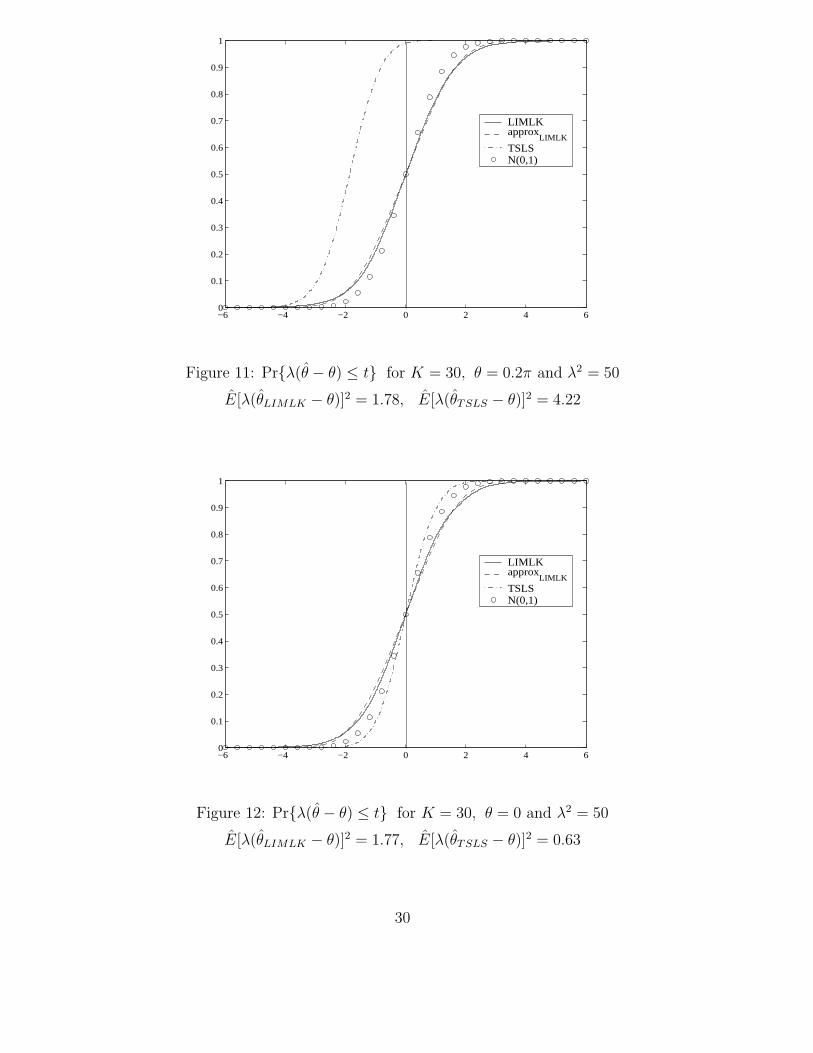
Figure 11: Pr{λ(θ − θ) ≤ t} for K = 30, θ = 0.2π and λ2 = 50
E[λ(θLIMLK − θ)]2 = 1.78, E[λ(θTSLS − θ)]2 = 4.22
−6 −4 −2 0 2 4 60
0.1
0.2
0.3
0.4
0.5
0.6
0.7
0.8
0.9
1
LIMLKapprox
LIMLKTSLSN(0,1)
Figure 12: Pr{λ(θ − θ) ≤ t} for K = 30, θ = 0 and λ2 = 50
E[λ(θLIMLK − θ)]2 = 1.77, E[λ(θTSLS − θ)]2 = 0.63
30

−6 −4 −2 0 2 4 60
0.1
0.2
0.3
0.4
0.5
0.6
0.7
0.8
0.9
1
LIMLKTSLSN(0,1)
Figure 13: Pr{λ(θ − θ) ≤ t} for K = 3, θ = 0.4π and λ2 = 10
E[λ(θLIMLK − θ)]2 = 1.56, E[λ(θTSLS − θ)]2 = 5.38
−6 −4 −2 0 2 4 60
0.1
0.2
0.3
0.4
0.5
0.6
0.7
0.8
0.9
1
LIMLKTSLSN(0,1)
Figure 14: Pr{λ(θ − θ) ≤ t} for K = 3, θ = 0.2π and λ2 = 10
E[λ(θLIMLK − θ)]2 = 1.58, E[λ(θTSLS − θ)]2 = 1.22
31

−6 −4 −2 0 2 4 60
0.1
0.2
0.3
0.4
0.5
0.6
0.7
0.8
0.9
1
LIMLKTSLSN(0,1)
Figure 15: Pr{λ(θ − θ) ≤ t} for K = 3, θ = 0 and λ2 = 10
E[λ(θLIMLK − θ)]2 = 1.57, E[λ(θTSLS − θ)]2 = 0.88
−6 −4 −2 0 2 4 60
0.1
0.2
0.3
0.4
0.5
0.6
0.7
0.8
0.9
1
LIMLKTSLSN(0,1)
Figure 16: Pr{λ(θ − θ) ≤ t} for K = 30, θ = 0.4π and λ2 = 10
E[λ(θLIMLK − θ)]2 = 4.06, E[λ(θTSLS − θ)]2 = 13.9
32

−6 −4 −2 0 2 4 60
0.1
0.2
0.3
0.4
0.5
0.6
0.7
0.8
0.9
1
LIMLKTSLSN(0,1)
Figure 17: Pr{λ(θ − θ) ≤ t} for K = 30, θ = 0.2π and λ2 = 10
E[λ(θLIMLK − θ)]2 = 3.90, E[λ(θTSLS − θ)]2 = 2.80
−6 −4 −2 0 2 4 60
0.1
0.2
0.3
0.4
0.5
0.6
0.7
0.8
0.9
1
LIMLKTSLSN(0,1)
Figure 18: Pr{λ(θ − θ) ≤ t} for K = 30, θ = 0 and λ2 = 10
E[λ(θLIMLK − θ)]2 = 3.93, E[λ(θTSLS − θ)]2 = 0.25
33