The Likelihood Ratio Test in High-Dimensional LogisticRegression Is Asymptotically a Rescaled Chi-Square

Pragya Sur∗ Yuxin Chen† Emmanuel J. Candès∗‡

June 2017; Revised August 2018

Abstract

Logistic regression is used thousands of times a day to fit data, predict future outcomes, and assess thestatistical significance of explanatory variables. When used for the purpose of statistical inference, logisticmodels produce p-values for the regression coefficients by using an approximation to the distribution ofthe likelihood-ratio test (LRT). Indeed, Wilks’ theorem asserts that whenever we have a fixed number pof variables, twice the log-likelihood ratio (LLR) 2Λ is distributed as a χ2

k variable in the limit of largesample sizes n; here, χ2

k is a chi-square with k degrees of freedom and k the number of variables beingtested. In this paper, we prove that when p is not negligible compared to n, Wilks’ theorem does nothold and that the chi-square approximation is grossly incorrect; in fact, this approximation producesp-values that are far too small (under the null hypothesis).

Assume that n and p grow large in such a way that p/n→ κ for some constant κ < 1/2. (For κ > 1/2,2Λ

P→ 0 so that the LRT is not interesting in this regime.) We prove that for a class of logistic models, theLLR converges to a rescaled chi-square, namely, 2Λ

d→ α(κ)χ2k, where the scaling factor α(κ) is greater

than one as soon as the dimensionality ratio κ is positive. Hence, the LLR is larger than classicallyassumed. For instance, when κ = 0.3, α(κ) ≈ 1.5. In general, we show how to compute the scalingfactor by solving a nonlinear system of two equations with two unknowns. Our mathematical argumentsare involved and use techniques from approximate message passing theory, from non-asymptotic randommatrix theory and from convex geometry. We also complement our mathematical study by showing thatthe new limiting distribution is accurate for finite sample sizes.

Finally, all the results from this paper extend to some other regression models such as the probitregression model.Keywords. Logistic regression, likelihood-ratio tests, Wilks’ theorem, high-dimensionality, goodness offit, approximate message passing, concentration inequalities, convex geometry, leave-one-out analysis

1 Introduction

Logistic regression is by far the most widely used tool for relating a binary response to a family of explanatoryvariables. This model is used to infer the importance of variables and nearly all standard statistical softwareshave inbuilt packages for obtaining p-values for assessing the significance of their coefficients. For instance,one can use the snippet of R code below to fit a logistic regression model from a vector y of binary responsesand a matrix X of covariates:

fitted <- glm(y ~ X+0, family = ‘binomial’)pvals <- summary(fitted)$coefficients[,4]

∗Department of Statistics, Stanford University, Stanford, CA 94305, U.S.A.†Department of Electrical Engineering, Princeton University, Princeton, NJ 08544, U.S.A.‡Department of Mathematics, Stanford University, Stanford, CA 94305, U.S.A.

1

The vector pvals stores p-values for testing whether a variable belongs to a model or not, and it is well knownthat the underlying calculations used to produce these p-values can also be used to construct confidenceintervals for the regression coefficients. Since logistic models are used hundreds of times every day forinference purposes, it is important to know whether these calculations—e.g. these p-values—are accurateand can be trusted.

1.1 Binary regressionImagine we have n samples of the form (yi,Xi), where yi ∈ 0, 1 and Xi ∈ Rp. In a generalized linearmodel, one postulates the existence of a link function µ(·) relating the conditional mean of the responsevariable to the linear predictor X>i β,

E[yi|Xi] = µ(X>i β), (1)

where β = [β1,β2, . . . ,βp]> ∈ Rp is an unknown vector of parameters. We focus here on the two most

commonly used binary regression models, namely, the logistic and the probit models for which

µ(t) :=

et/(1 + et) in the logistic model,Φ(t) in the probit model;

(2)

here, Φ is the cumulative distribution function (CDF) of a standard normal random variable. In both cases,the Symmetry Condition

µ(t) + µ(−t) = 1 (3)

holds, which says that the two types yi = 0 and yi = 1 are treated in a symmetric fashion. Assuming thatthe observations are independent, the negative log-likelihood function is given by [1, Section 4.1.2]

` (β) := −n∑i=1

yi log

(µi

1− µi

)+ log (1− µi)

, µi := µ(X>i β).

Invoking the symmetry condition, a little algebra reveals an equivalent expression

` (β) :=∑n

i=1ρ(− yiX>i β

), (4)

where

yi :=

1 if yi = 1,

−1 if yi = 0,and ρ(t) :=

log (1 + et) in the logistic case,− log Φ (−t) in the probit case.

(5)

Throughout we refer to this function ρ as the effective link.

1.2 The likelihood-ratio test and Wilks’ phenomenonResearchers often wish to determine which covariates are of importance, or more precisely, to test whetherthe jth variable belongs to the model or not: formally, we wish to test the hypothesis

Hj : βj = 0 versus βj 6= 0. (6)

Arguably, one of the most commonly deployed techniques for testing Hj is the likelihood-ratio test (LRT),which is based on the log-likelihood ratio (LLR) statistic

Λj := `(β(−j)

)− `(β). (7)

Here, β and β(−j) denote respectively the maximum likelihood estimates (MLEs) under the full model andthe reduced model on dropping the jth predictor; that is,

β = arg minβ∈Rp

`(β) and β(−j) = arg minβ∈Rp,βj=0

`(β).

2

Inference based on such log-likelihood ratio statistics has been studied extensively in prior literature [13,44,66]. Arguably, one of the most celebrated results in the large-sample regime is the Wilks’ theorem.

To describe the Wilks’ phenomenon, imagine we have a sequence of observations (yi,Xi) where yi ∈ 0, 1,Xi ∈ Rp with p fixed. Since we are interested in the limit of large samples, we may want to assume that thecovariates are i.i.d. drawn from some population with non-degenerate covariance matrix so that the problemis fully p-dimensional. As before, we assume a conditional logistic model for the response. In this setting,Wilks’ theorem [66] calculates the asymptotic distribution of Λj(n) when n grows to infinity:

(Wilks’ phenomenon) Under suitable regularity conditions which, for instance, guarantee that theMLE exists and is unique,1 the LLR statistic for testing Hj : βj = 0 vs. βj 6= 0 has asymptoticdistribution under the null given by

2Λj(n)d→ χ2

1, as n→∞. (8)

This fixed-p large-n asymptotic result, which is a consequence of asymptotic normality properties of theMLE [64, Theorem 5.14], applies to a much broader class of testing problems in parametric models; forinstance, it applies to the probit model as well. We refer the readers to [41, Chapter 12] and [64, Chapter16] for a thorough exposition and details on the regularity conditions under which Wilks’ theorem holds.Finally, there is a well-known extension which states that if we were to drop k variables from the model,then the LLR would converge to a chi-square distribution with k degrees of freedom under the hypothesisthat the reduced model is correct.

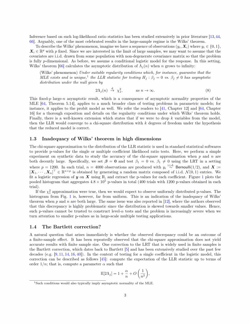
1.3 Inadequacy of Wilks’ theorem in high dimensionsThe chi-square approximation to the distribution of the LLR statistic is used in standard statistical softwaresto provide p-values for the single or multiple coefficient likelihood ratio tests. Here, we perform a simpleexperiment on synthetic data to study the accuracy of the chi-square approximation when p and n areboth decently large. Specifically, we set β = 0 and test β1 = 0 vs. β1 6= 0 using the LRT in a settingwhere p = 1200. In each trial, n = 4000 observations are produced with yi

i.i.d.∼ Bernoulli(1/2), and X :=[X1, · · · ,Xn]> ∈ Rn×p is obtained by generating a random matrix composed of i.i.d. N (0, 1) entries. Wefit a logistic regression of y on X using R, and extract the p-values for each coefficient. Figure 1 plots thepooled histogram that aggregates 4.8× 105 p-values in total (400 trials with 1200 p-values obtained in eachtrial).

If the χ21 approximation were true, then we would expect to observe uniformly distributed p-values. The

histrogram from Fig. 1 is, however, far from uniform. This is an indication of the inadequacy of Wilks’theorem when p and n are both large. The same issue was also reported in [12], where the authors observedthat this discrepancy is highly problematic since the distribution is skewed towards smaller values. Hence,such p-values cannot be trusted to construct level-α tests and the problem is increasingly severe when weturn attention to smaller p-values as in large-scale multiple testing applications.

1.4 The Bartlett correction?A natural question that arises immediately is whether the observed discrepancy could be an outcome ofa finite-sample effect. It has been repeatedly observed that the chi-square approximation does not yieldaccurate results with finite sample size. One correction to the LRT that is widely used in finite samples isthe Bartlett correction, which dates back to Bartlett [5] and has been extensively studied over the past fewdecades (e.g. [9, 11, 14, 16, 40]). In the context of testing for a single coefficient in the logistic model, thiscorrection can be described as follows [45]: compute the expectation of the LLR statistic up to terms oforder 1/n; that is, compute a parameter α such that

E[2Λj ] = 1 +α

n+O

(1

n2

),

1Such conditions would also typically imply asymptotic normality of the MLE.

3

0

10000

20000

30000

0.00 0.25 0.50 0.75 1.00P−Values

Cou

nts

0

5000

10000

15000

0.00 0.25 0.50 0.75 1.00P−Values

Cou

nts

0

2500

5000

7500

10000

12500

0.00 0.25 0.50 0.75 1.00P−Values

Cou

nts

(a) (b) (c)

Figure 1: Histogram of p-values for logistic regression under i.i.d. Gaussian design, when β = 0, n = 4000,p = 1200, and κ = 0.3: (a) classically computed p-values; (b) Bartlett-corrected p-values; (c) adjustedp-values by comparing the LLR to the rescaled chi square α(κ)χ2

1 (27).

which suggests a corrected LLR statistic2Λj

1 + αnn

(9)

with αn being an estimator of α. With a proper choice of αn, one can ensure

E[

2Λj1 + αn

n

]= 1 +O

(1

n2

)in the classical setting where p is fixed and n diverges. In expectation, this corrected statistic is closer to aχ2

1 distribution than the original LLR for finite samples. Notably, the correction factor may in general be afunction of the unknown β and, in that case, must be estimated from the null model via maximum likelihoodestimation.

In the context of GLMs, Cordeiro [14] derived a general formula for the Bartlett corrected LLR statistic,see [15, 20] for a detailed survey. In the case where there is no signal (β = 0), one can compute αn for thelogistic regression model following [14] and [45], which yields

αn =n

2

[Tr(D2p

)− Tr

(D2p−1

)]. (10)

Here, Dp is the diagonal part of X(X>X)−1X> and Dp−1 is that of X(−j)(X>(−j)X(−j)

)−1X>(−j) in

which X(−j) is the design matrix X with the jth column removed. Comparing the adjusted LLRs to a χ21

distribution yields adjusted p-values. In the setting of Fig. 1(a), the histogram of Bartlett corrected p-valuesis shown in Fig. 1(b). As we see, these p-values are still far from uniform.

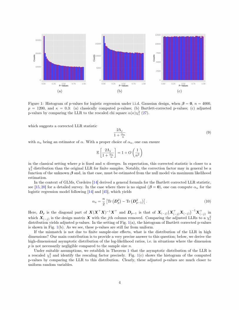
If the mismatch is not due to finite sample-size effects, what is the distribution of the LLR in highdimensions? Our main contribution is to provide a very precise answer to this question; below, we derive thehigh-dimensional asymptotic distribution of the log-likelihood ratios, i.e. in situations where the dimensionp is not necessarily negligible compared to the sample size n.

Under suitable assumptions, we establish in Theorem 1 that the asymptotic distribution of the LLR isa rescaled χ2

1 and identify the rescaling factor precisely. Fig. 1(c) shows the histogram of the computedp-values by comparing the LLR to this distribution. Clearly, these adjusted p-values are much closer touniform random variables.

4

2 Main results

2.1 Modelling assumptionsIn this paper, we focus on the high-dimensional regime where the sample size is not much larger than thenumber of parameters to be estimated—a setting which has attracted a flurry of activity in recent years.In particular, we assume that the number p(n) of covariates grows proportionally with the number n ofobservations; that is,

limn→∞

p(n)

n= κ, (11)

where κ > 0 is a fixed constant independent of n and p(n). In fact, we shall also assume κ < 1/2 for boththe logistic and the probit models, as the MLE does not exist otherwise; see Section 2.2.

To formalize the notion of high-dimensional asymptotics when both n and p(n) diverge, we consider asequence of instances X(n),y(n)n≥0 such that for any n,

• X(n) ∈ Rn×p(n) has i.i.d. rows Xi(n) ∼ N (0, Σ), where Σ ∈ Rp(n)×p(n) is positive definite;

• yi(n) |X(n) ∼ yi(n) |Xi(n)ind.∼ Bernoulli

(µ(Xi(n)>β(n))

), where µ satisfies the Symmetry Condition;

• we further assume β(n) = 0. From the Symmetry Condition it follows that µ(0) = 1/2, which directlyimplies that y(n) is a vector with i.i.d Bernoulli(1/2) entries.

The MLE is denoted by β(n) and there are p(n) LLR statistics Λj(n) (1 ≤ j ≤ p(n)), one for each of thep(n) regression coefficients. In the sequel, the dependency on n shall be suppressed whenever it is clear fromthe context.

2.2 When does the MLE exist?Even though we are operating in the regime where n > p, the existence of the MLE cannot be guaranteedfor all p and n. Interestingly, the norm of the MLE undergoes a sharp phase transition in the sense thatwith high probability,

‖β‖ =∞ if κ > 1/2; (12)

‖Σ1/2β‖ = O(1) if κ < 1/2. (13)

The first result (12) concerns the separating capacity of linear inequalities, which dates back to Cover’sPh. D. thesis [17]. Specifically, given that ρ(t) ≥ ρ(−∞) = 0 for both the logistic and probit models, eachsummand in (4) is minimized if yiX>i β = ∞, which occurs when sign(X>i β) = sign(yi) and ‖β‖ = ∞. Asa result, if there exists a nontrivial ray β such that

X>i β > 0 if yi = 1 and X>i β < 0 if yi = −1 (14)

for any 1 ≤ i ≤ n, then pushing ‖β‖ to infinity leads to an optimizer of (4). In other words, the solution to(4) becomes unbounded (the MLE is at ∞) whenever there is a hyperplane perfectly separating the two setsof samples i | yi = 1 and i | yi = −1. According to [17, 18], the probability of separability tends to onewhen κ > 1/2, in which case the MLE does not exist. This separability result was originally derived usingclassical combinatorial geometry.

The current paper follows another route by resorting to convex geometry, which, as we will demonstratelater, also tells us how to control the norm of the MLE when κ < 1/2.2 To begin with, we observe that yi isindependent of X and the distribution of X is symmetric under the assumptions from Section 2.1. Hence,

2The separability results in [17,18] do not imply the control on the norm of the MLE when κ < 1/2.

5

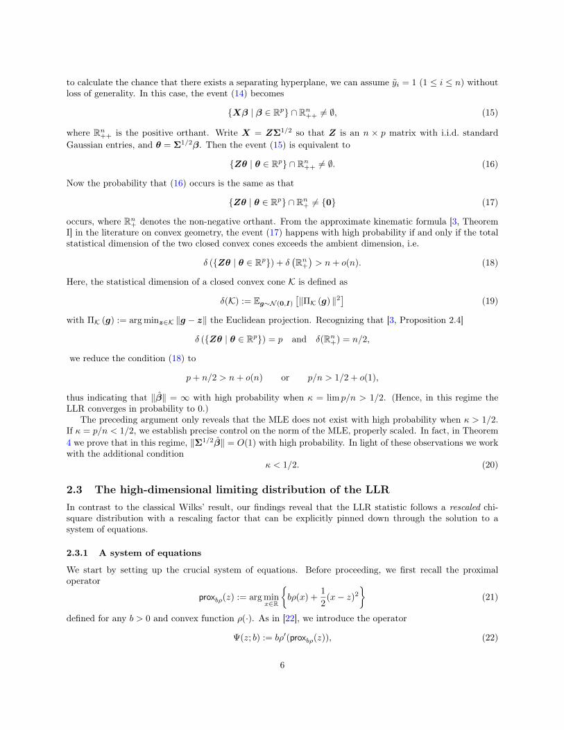
to calculate the chance that there exists a separating hyperplane, we can assume yi = 1 (1 ≤ i ≤ n) withoutloss of generality. In this case, the event (14) becomes

Xβ | β ∈ Rp ∩ Rn++ 6= ∅, (15)

where Rn++ is the positive orthant. Write X = ZΣ1/2 so that Z is an n × p matrix with i.i.d. standardGaussian entries, and θ = Σ1/2β. Then the event (15) is equivalent to

Zθ | θ ∈ Rp ∩ Rn++ 6= ∅. (16)

Now the probability that (16) occurs is the same as that

Zθ | θ ∈ Rp ∩ Rn+ 6= 0 (17)

occurs, where Rn+ denotes the non-negative orthant. From the approximate kinematic formula [3, TheoremI] in the literature on convex geometry, the event (17) happens with high probability if and only if the totalstatistical dimension of the two closed convex cones exceeds the ambient dimension, i.e.

δ (Zθ | θ ∈ Rp) + δ(Rn+)> n+ o(n). (18)

Here, the statistical dimension of a closed convex cone K is defined as

δ(K) := Eg∼N (0,I)

[‖ΠK (g) ‖2

](19)

with ΠK (g) := arg minz∈K ‖g − z‖ the Euclidean projection. Recognizing that [3, Proposition 2.4]

δ (Zθ | θ ∈ Rp) = p and δ(Rn+) = n/2,

we reduce the condition (18) to

p+ n/2 > n+ o(n) or p/n > 1/2 + o(1),

thus indicating that ‖β‖ = ∞ with high probability when κ = lim p/n > 1/2. (Hence, in this regime theLLR converges in probability to 0.)

The preceding argument only reveals that the MLE does not exist with high probability when κ > 1/2.If κ = p/n < 1/2, we establish precise control on the norm of the MLE, properly scaled. In fact, in Theorem4 we prove that in this regime, ‖Σ1/2β‖ = O(1) with high probability. In light of these observations we workwith the additional condition

κ < 1/2. (20)

2.3 The high-dimensional limiting distribution of the LLRIn contrast to the classical Wilks’ result, our findings reveal that the LLR statistic follows a rescaled chi-square distribution with a rescaling factor that can be explicitly pinned down through the solution to asystem of equations.

2.3.1 A system of equations

We start by setting up the crucial system of equations. Before proceeding, we first recall the proximaloperator

proxbρ(z) := arg minx∈R

bρ(x) +

1

2(x− z)2

(21)

defined for any b > 0 and convex function ρ(·). As in [22], we introduce the operator

Ψ(z; b) := bρ′(proxbρ(z)), (22)

6

which is simply the proximal operator of the conjugate (bρ)∗ of bρ.3 To see this, we note that Ψ satisfies therelation [22, Proposition 6.4]

Ψ(z; b) + proxbρ(z) = z. (23)

The claim that Ψ(·; b) = prox(bρ)∗(·) then follows from the Moreau decomposition

proxf (z) + proxf∗(z) = z, ∀z, (24)

which holds for a closed convex function f [47, Section 2.5]. Interested readers are referred to [22, Appendix1] for more properties of proxbρ and Ψ.

We are now in position to present the system of equations that plays a crucial role in determining thedistribution of the LLR statistic in high dimensions:

τ2 =1

κE[(Ψ (τZ; b))

2]

, (25)

κ = E[Ψ′ (τZ; b)

], (26)

where Z ∼ N (0, 1), and Ψ′ (·, ·) denotes differentiation with respect to the first variable. The fact that thissystem of equations would admit a unique solution in R2

+ is not obvious a priori. We shall establish this forthe logistic and the probit models later in Section 6.

2.3.2 Main result

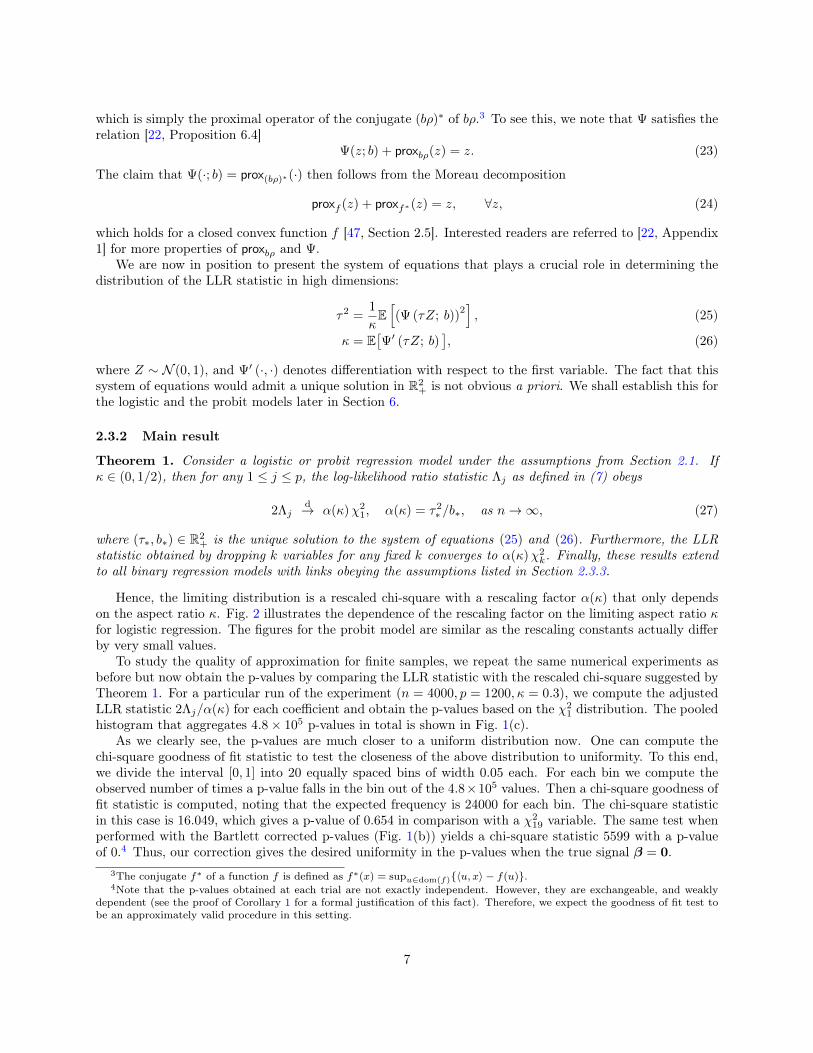
Theorem 1. Consider a logistic or probit regression model under the assumptions from Section 2.1. Ifκ ∈ (0, 1/2), then for any 1 ≤ j ≤ p, the log-likelihood ratio statistic Λj as defined in (7) obeys

2Λjd→ α(κ)χ2

1, α(κ) = τ2∗ /b∗, as n→∞, (27)

where (τ∗, b∗) ∈ R2+ is the unique solution to the system of equations (25) and (26). Furthermore, the LLR

statistic obtained by dropping k variables for any fixed k converges to α(κ)χ2k. Finally, these results extend

to all binary regression models with links obeying the assumptions listed in Section 2.3.3.

Hence, the limiting distribution is a rescaled chi-square with a rescaling factor α(κ) that only dependson the aspect ratio κ. Fig. 2 illustrates the dependence of the rescaling factor on the limiting aspect ratio κfor logistic regression. The figures for the probit model are similar as the rescaling constants actually differby very small values.

To study the quality of approximation for finite samples, we repeat the same numerical experiments asbefore but now obtain the p-values by comparing the LLR statistic with the rescaled chi-square suggested byTheorem 1. For a particular run of the experiment (n = 4000, p = 1200,κ = 0.3), we compute the adjustedLLR statistic 2Λj/α(κ) for each coefficient and obtain the p-values based on the χ2

1 distribution. The pooledhistogram that aggregates 4.8× 105 p-values in total is shown in Fig. 1(c).

As we clearly see, the p-values are much closer to a uniform distribution now. One can compute thechi-square goodness of fit statistic to test the closeness of the above distribution to uniformity. To this end,we divide the interval [0, 1] into 20 equally spaced bins of width 0.05 each. For each bin we compute theobserved number of times a p-value falls in the bin out of the 4.8×105 values. Then a chi-square goodness offit statistic is computed, noting that the expected frequency is 24000 for each bin. The chi-square statisticin this case is 16.049, which gives a p-value of 0.654 in comparison with a χ2

19 variable. The same test whenperformed with the Bartlett corrected p-values (Fig. 1(b)) yields a chi-square statistic 5599 with a p-valueof 0.4 Thus, our correction gives the desired uniformity in the p-values when the true signal β = 0.

3The conjugate f∗ of a function f is defined as f∗(x) = supu∈dom(f)〈u,x〉 − f(u).4Note that the p-values obtained at each trial are not exactly independent. However, they are exchangeable, and weakly

dependent (see the proof of Corollary 1 for a formal justification of this fact). Therefore, we expect the goodness of fit test tobe an approximately valid procedure in this setting.

7

1.00

1.25

1.50

1.75

2.00

0.00 0.05 0.10 0.15 0.20 0.25 0.30 0.35 0.40κ

Res

calin

g C

onst

ant

1.0

2.5

5.0

10.0

15.0

20.0

25.0

0.00 0.05 0.10 0.15 0.20 0.25 0.30 0.35 0.40 0.45κ

Res

calin

g C

onst

ant

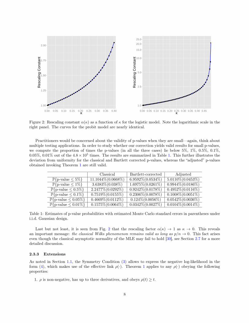
Figure 2: Rescaling constant α(κ) as a function of κ for the logistic model. Note the logarithmic scale in theright panel. The curves for the probit model are nearly identical.

Practitioners would be concerned about the validity of p-values when they are small—again, think aboutmultiple testing applications. In order to study whether our correction yields valid results for small p-values,we compute the proportion of times the p-values (in all the three cases) lie below 5%, 1%, 0.5%, 0.1%,0.05%, 0.01% out of the 4.8× 105 times. The results are summarized in Table 1. This further illustrates thedeviation from uniformity for the classical and Bartlett corrected p-values, whereas the “adjusted” p-valuesobtained invoking Theorem 1 are still valid.

Classical Bartlett-corrected AdjustedPp-value ≤ 5% 11.1044%(0.0668%) 6.9592%(0.0534%) 5.0110%(0.0453%)Pp-value ≤ 1% 3.6383%(0.038%) 1.6975%(0.0261%) 0.9944%(0.0186%)Pp-value ≤ 0.5% 2.2477%(0.0292%) 0.9242%(0.0178%) 0.4952%(0.0116%)Pp-value ≤ 0.1% 0.7519%(0.0155%) 0.2306%(0.0078%) 0.1008%(0.0051%)Pp-value ≤ 0.05% 0.4669%(0.0112%) 0.124%(0.0056%) 0.0542%(0.0036%)Pp-value ≤ 0.01% 0.1575%(0.0064%) 0.0342%(0.0027%) 0.0104%(0.0014%)

Table 1: Estimates of p-value probabilities with estimated Monte Carlo standard errors in parentheses underi.i.d. Gaussian design.

Last but not least, it is seen from Fig. 2 that the rescaling factor α(κ) → 1 as κ → 0. This revealsan important message: the classical Wilks phenomenon remains valid as long as p/n → 0. This fact ariseseven though the classical asymptotic normality of the MLE may fail to hold [30], see Section 2.7 for a moredetailed discussion.

2.3.3 Extensions

As noted in Section 1.1, the Symmetry Condition (3) allows to express the negative log-likelihood in theform (4), which makes use of the effective link ρ(·). Theorem 1 applies to any ρ(·) obeying the followingproperties:

1. ρ is non-negative, has up to three derivatives, and obeys ρ(t) ≥ t.

8

2. ρ′ may be unbounded but it should grow sufficiently slowly, in particular, we assume |ρ′(t)| = O(|t|)and ρ′(proxcρ(Z)) is a sub-Gaussian random variable for any constant c > 0 and any Z ∼ N (0,σ2) forsome finite σ > 0.

3. ρ′′(t) > 0 for any t which implies that ρ is convex, and supt ρ′′(t) <∞.

4. supt |ρ′′′(t)| <∞.

5. Given any τ > 0 ,the equation (26) has a unique solution in b.

6. The map V(τ2) as defined in (59) has a fixed point.

It can be checked that the effective links for both the logistic and the probit models (5) obey all of the above.The last two conditions are assumed to ensure existence of a unique solution to the system of equations (25)and (26) as will be seen in Section 6; we shall justify these two conditions for the logistic and the probitmodels in Section 6.1.

2.4 Reduction to independent covariatesIn order to derive the asymptotic distribution of the LLR statistics, it in fact suffices to consider the specialcase Σ = Ip.

Lemma 1. Let Λj(X) be the LLR statistic based on the design matrix X, where the rows of X arei.i.d. N (0, Σ) and Λj(Z) that where the rows are i.i.d. N (0, Ip). Then

Λj(X)d= Λj(Z).

Proof: Recall from (4) that the LLR statistic for testing the jth coefficient can be expressed as

Λj(X) = minβ

n∑i=1

ρ(−yie>i Xβ)− minβ:βj=0

n∑i=1

ρ(−yie>i Xβ).

Write Z ′ = XΣ−1/2 so that the rows of Z ′ are i.i.d. N (0, Ip) and set θ′ = Σ1/2β. With this reparameter-ization, we observe that the constraint βj = 0 is equivalent to a>j θ′ = 0 for some non-zero vector aj ∈ Rp.This gives

Λj(X) = minθ′

n∑i=1

ρ(−yie>i Z ′θ′)− minθ′:a>j θ

′=0

n∑i=1

ρ(−yie>i Z ′θ′).

Now let Q be an orthogonal matrix mapping aj ∈ Rp into the vector ‖aj‖ej ∈ Rp, i.e. Qaj = ‖aj‖ej .Additionally, set Z = Z ′Q (the rows of Z are still i.i.d. N (0, Ip)) and θ = Qθ′. Since a>j θ′ = 0 occurs ifand only if θj = 0, we obtain

Λj(X) = minθ

n∑i=1

ρ(−yie>i Zθ)− minθ:θj=0

n∑i=1

ρ(−yie>i Zθ) = Λj(Z),

which proves the lemma.

In the remainder of the paper we, therefore, assume Σ = Ip.

2.5 Proof architectureThis section presents the main steps for proving Theorem 1. We will only prove the theorem for Λj, theLLR statistic obtained by dropping a single variable. The analysis for the LLR statistic obtained on droppingk variables (for some fixed k) follows very similar steps and is hence omitted for the sake of conciseness. Asdiscussed before, we are free to work with any configuration of the yi’s. For the two steps below, we willadopt two different configurations for convenience of presentation.

9

2.5.1 Step 1: characterizing the asymptotic distributions of βj

Without loss of generality, we assume here that yi = 1 (and hence yi = 1) for all 1 ≤ i ≤ n and, therefore,the MLE problem reduces to

minimizeβ∈Rp∑n

i=1ρ(−X>i β).

We would first like to characterize the marginal distribution of β, which is crucial in understanding theLLR statistic. To this end, our analysis follows by a reduction to the setup of [22, 24–26], with certainmodifications that are called for due to the specific choices of ρ(·) we deal with here. Specifically, considerthe linear model

y = Xβ +w, (28)

and prior work [22,24–26] investigating the associated M-estimator

minimizeβ∈Rp∑n

i=1ρ(yi −X>i β). (29)

Our problem reduces to (29) on setting y = w = 0 in (29). When ρ(·) satisfies certain assumptions(e.g. strong convexity), the asymptotic distribution of ‖β‖ has been studied in a series of works [24–26] usinga leave-one-out analysis and independently in [22] using approximate message passing (AMP) machinery.An outline of their main results is described in Section 2.7. However, the function ρ(·) in our cases hasvanishing curvature and, therefore, lacks the essential strong convexity assumption that was utilized in boththe aforementioned lines of work. To circumvent this issue, we propose to invoke the AMP machinery asin [22], in conjunction with the following critical additional ingredients:

• (Norm Bound Condition) We utilize results from the conic geometry literature (e.g. [3]) to establishthat

‖β‖ = O(1)

with high probability as long as κ < 1/2. This will be elaborated in Theorem 4.

• (Likelihood Curvature Condition) We establish some regularity conditions on the Hessian of the log-likelihood function, generalizing the strong convexity condition, which will be detailed in Lemma 4.

• (Uniqueness of the Solution to (25) and (26)) We establish that for both the logistic and the probitcase, the system of equations (25) and (26) admits a unique solution.

We emphasize that these elements are not straightforward, require significant effort and a number of novelideas, which form our primary technical contributions for this step.

These ingredients enable the use of the AMP machinery even in the absence of strong convexity on ρ(·),finally leading to the following theorem:

Theorem 2. Under the conditions of Theorem 1,

limn→∞

‖β‖2 =a.s. τ2∗ . (30)

This theorem immediately implies that the marginal distribution of βj is normal.

Corollary 1. Under the conditions of Theorem 1, for every 1 ≤ j ≤ p, it holds that

√pβj

d→ N (0, τ2∗ ), as n→∞. (31)

Proof: From the rotational invariance of our i.i.d. Gaussian design, it can be easily verified that β/‖β‖is uniformly distributed on the unit sphere Sp−1 and is independent of ‖β‖. Therefore, βj has the samedistribution as ‖β‖Zj/‖Z‖, where Z = (Z1, . . . ,Zp) ∼ N (0, Ip) independent of ‖β‖. Since √p‖β‖/‖Z‖converges in probability to τ∗, we have, by Slutsky’s theorem, that√pβj converges toN (0, τ2

∗ ) in distribution.

10

2.5.2 Step 2: connecting Λj with βj

Now that we have derived the asymptotic distribution of βj , the next step involves a reduction of the LLRstatistic to a function of the relevant coordinate of the MLE. Before continuing, we note that the distributionof Λj is the same for all 1 ≤ j ≤ p due to exchangeability. As a result, going forward we will only analyzeΛ1 without loss of generality. In addition, we introduce the following convenient notations and assumptions:

• the design matrix on dropping the first column is written as X and the MLE in the correspondingreduced model as β;

• write X = [X1, · · · ,Xn]> ∈ Rn×p and X = [X1, · · · , Xn]> ∈ Rn×(p−1);

• without loss of generality, assume that yi = −1 for all i in this subsection, and hence the MLEs underthe full and the reduced models reduce to

β = arg minβ∈Rp `(β) :=∑n

i=1ρ(X>i β), (32)

β = arg minβ∈Rp−1˜(β) :=

∑n

i=1ρ(X>i β). (33)

With the above notations in place, the LLR statistic for testing β1 = 0 vs. β1 6= 0 can be expressed as

Λ1 := ˜(β)− `(β) =

n∑i=1

ρ(X>i β)− ρ(X>i β)

. (34)

To analyze Λ1, we invoke Taylor expansion to reach

Λ1 =

n∑i=1

ρ′(X>i β

)(X>i β −X>i β

)︸ ︷︷ ︸

:=Qlin

+1

2

n∑i=1

ρ′′(X>i β

)(X>i β −X>i β

)2

+1

6

n∑i=1

ρ′′′(γi)(X>i β −X>i β

)3

, (35)

where γi lies between X>i β and X>i β. A key observation is that the linear term Qlin in the above equationvanishes. To see this, note that the first-order optimality conditions for the MLE β is given by∑n

i=1ρ′(X>i β)Xi = 0. (36)

Replacing X>i β with X>i

[0

β

]in Qlin and using the optimality condition, we obtain

Qlin =(∑n

i=1ρ′(X>i β

)Xi

)>([ 0

β

]− β

)= 0.

Consequently, Λ1 simplifies to the following form

Λ1 =1

2

n∑i=1

ρ′′(X>i β)(X>i β −X>i β

)2

+1

6

n∑i=1

ρ′′′(γi)(X>i β −X>i β

)3

. (37)

Thus, computing the asymptotic distribution of Λ1 boils down to analyzing X>i β− X>i β. Our argument isinspired by the leave-one-predictor-out approach developed in [24,25].

We re-emphasize that our setting is not covered by that of [24,25], due to the violation of strong convexityand some other technical assumptions. We sidestep this issue by utilizing the Norm Bound Condition andthe Likelihood Curvature Condition. In the end, our analysis establishes the equivalence of Λ1 and β1 up tosome explicit multiplicative factors modulo negligible error terms. This is summarized as follows.

11

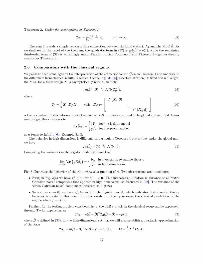
Theorem 3. Under the assumptions of Theorem 1,

2Λ1 −p

b∗β2

1P→ 0, as n→∞. (38)

Theorem 3 reveals a simple yet surprising connection between the LLR statistic Λ1 and the MLE β. Aswe shall see in the proof of the theorem, the quadratic term in (37) is 1

2pb∗β2

1 + o(1), while the remainingthird-order term of (37) is vanishingly small. Finally, putting Corollary 1 and Theorem 3 together directlyestablishes Theorem 1.

2.6 Comparisons with the classical regime

We pause to shed some light on the interpretation of the correction factor τ2∗ /b∗ in Theorem 1 and understand

the differences from classical results. Classical theory (e.g. [35,36]) asserts that when p is fixed and n diverges,the MLE for a fixed design X is asymptotically normal, namely,

√n(β − β)

d→ N (0, I−1β ), (39)

where

Iβ =1

nX>DβX with Dβ :=

ρ′′(X>1 β

). . .

ρ′′(X>n β

) (40)

is the normalized Fisher information at the true value β. In particular, under the global null and i.i.d. Gaus-sian design, this converges to

EX [Iβ] =

14I, for the logistic model2πI, for the probit model

as n tends to infinity [64, Example 5.40].The behavior in high dimensions is different. In particular, Corollary 1 states that under the global null,

we have √p(βj − βj)

d→ N (0, τ2∗ ). (41)

Comparing the variances in the logistic model, we have that

limn→∞

Var(√

pβj

)=

4κ, in classical large-sample theory;

τ2∗ , in high dimensions.

Fig. 3 illustrates the behavior of the ratio τ2∗ /κ as a function of κ. Two observations are immediate:

• First, in Fig. 3(a) we have τ2∗ ≥ 4κ for all κ ≥ 0. This indicates an inflation in variance or an “extra

Gaussian noise” component that appears in high dimensions, as discussed in [22]. The variance of the“extra Gaussian noise” component increases as κ grows.

• Second, as κ → 0, we have τ2∗ /4κ → 1 in the logistic model, which indicates that classical theory

becomes accurate in this case. In other words, our theory recovers the classical prediction in theregime where p = o(n).

Further, for the testing problem considered here, the LLR statistic in the classical setup can be expressed,through Taylor expansion, as

2Λ1 = n(β − β)>Iβ(β − β) + oP (1), (42)

where β is defined in (33). In the high-dimensional setting, we will also establish a quadratic approximationof the form

2Λ1 = n(β − β)>G(β − β) + oP (1), G =1

nX>DβX.

12

4

10

20

30

0.00 0.05 0.10 0.15 0.20 0.25 0.30 0.35 0.40κ

τ2κ

(a) logistic regression

1.57

2.5

5

7.5

10

0.00 0.05 0.10 0.15 0.20 0.25 0.30 0.35 0.40κ

τ2κ

(b) probit regression

Figure 3: Ratio of asymptotic variance and dimensionality factor κ as a function of κ.

In Theorem 7, we shall see that b∗ is the limit of 1nTr(G−1), the Stieltjes transform of the empirical spectral

distribution of G evaluated at 0. Thus, this quantity in some sense captures the spread in the eigenvaluesof G one would expect to happen in high dimensions.

2.7 Prior artWilks’ type of phenomenon in the presence of a diverging dimension p has received much attention in the past.For instance, Portnoy [51] investigated simple hypotheses in regular exponential families, and establishedthe asymptotic chi-square approximation for the LLR test statistic as long as p3/2/n→ 0. This phenomenonwas later extended in [54] to accommodate the MLE with a quadratic penalization, and in [67] to accountfor parametric models underlying several random graph models. Going beyond parametric inference, Fanet al. [27, 29] explored extensions to infinite-dimensional non-parametric inference problems, for which theMLE might not even exist or might be difficult to derive. While the classical Wilks’ phenomenon fails tohold in such settings, Fan et al. [27, 29] proposed a generalization of the likelihood ratio statistics basedon suitable non-parametric estimators and characterized the asymptotic distributions. Such results havefurther motivated Boucheron and Massart [10] to investigate the non-asymptotic Wilks’ phenomenon or,more precisely, the concentration behavior of the difference between the excess empirical risk and the truerisk, from a statistical learning theory perspective. The Wilks’ phenomenon for penalized empirical likelihoodhas also been established [59]. However, the precise asymptotic behavior of the LLR statistic in the regimethat permits p to grow proportional to n is still beyond reach.

On the other hand, as demonstrated in Section 2.5.1, the MLE here under the global null can be viewed asan M-estimator for a linear regression problem. Questions regarding the behavior of robust linear regressionestimators in high dimensions—where p is allowed to grow with n—–were raised in Huber [35], and havebeen extensively studied in subsequent works, e.g. [43, 48–50]. When it comes to logistic regression, thebehavior of the MLE was studied for a diverging number of parameters by [33], which characterized thesquared estimation error of the MLE if (p log p)/n→ 0. In addition, the asymptotic normality properties ofthe MLE and the penalized MLE for logistic regression have been established by [42] and [28], respectively.A very recent paper by Fan et al. [30] studied the logistic model under the global null β = 0, and investigatedthe classical asymptotic normality as given in (39). It was discovered in [30] that the convergence property

13

breaks down even in terms of the marginal distribution, namely,√nβi(

Iβ)−1/2

i,i

d9 N (0, 1) , Iβ =1

4nX>X,

as soon as p grows at a rate exceeding n2/3. In other words, classical theory breaks down. Having saidthis, when κ = p/n → 0, Wilks’ theorem still holds since Theorem 1 and Fig. 2 demonstrate that the LLRstatistic 2Λj converges in distribution to a chi-square.5

The line of work that is most relevant to the present paper was initially started by El Karoui et al. [26].Focusing on the regime where p is comparable to n, the authors uncovered, via a non-rigorous argument,that the asymptotic `2 error of the MLE could be characterized by a system of nonlinear equations. Thisseminal result was later made rigorous independently by Donoho et al. [22, 23] under i.i.d. Gaussian designand by El Karoui [24, 25] under more general i.i.d. random design as well as certain assumptions on theerror distribution. Both approaches rely on strong convexity on the function ρ(·) that defines the M-estimator, which does not hold in the models considered herein. The case of ridge regularized M-estimatorswere also studied in [24, 25]. Thrampoulidis et al. [61] studied the asymptotic behavior of the squarederror for regularized M-estimators for a broad class of regularizers. They also examined the unregularizedcase under more general assumptions on the loss function. Our setup is not covered by this work; severalconditions are violated including some pertaining to the growth rate of ρ′. We also have completely differenterror distributions since we are not working under the linear model as they are. Simultaneously, penalizedlikelihood procedures have been studied extensively under high-dimensional setups with sparsity constraintsimposed on the underlying signal; see, for instance, [37, 39,62,63] and the references cited therein.

Finally, we remark that the AMP machinery has already been successfully applied to study other statis-tical problems, including but not limited to the mean square estimation error of the Lasso [8], the tradeoffbetween the type I and type II errors along the Lasso path [55], and the hidden clique problem [21].

2.8 NotationsWe adopt the standard notation f(n) = O (g(n)) or f(n) . g(n) which means that there exists a constantc > 0 such that |f(n)| ≤ c|g(n)|. Likewise, f(n) = Ω (g(n)) or f(n) & g(n) means that there exists aconstant c > 0 such that |f(n)| ≥ c |g(n)|, f(n) g(n) means that there exist constants c1, c2 > 0 such thatc1|g(n)| ≤ |f(n)| ≤ c2|g(n)|, and f(n) = o(g(n)) means that limn→∞

f(n)g(n) = 0. Any mention of C, Ci, c, ci

for i ∈ N refers to some positive universal constants whose value may change from line to line. For a squaresymmetric matrix M , the minimum eigenvalue is denoted by λmin(M). Logarithms are base e.

3 Numerics

3.1 Non-Gaussian covariatesIn this section we first study the sensitivity of our result to the Gaussianity assumption on the design matrix.To this end, we consider a high dimensional binary regression set up with a Bernoulli design matrix. Wesimulate n = 4000 i.i.d. observations (yi,Xi) with yi

i.i.d.∼ Bernoulli(1/2), andXi generated independent of yi,such that each entry takes on values in 1,−1 w.p. 1/2. At each trial, we fit a logistic regression model tothe data and obtain the classical, Bartlett corrected and adjusted p-values (using the rescaling factor α(κ)).Figure 4 plots the histograms for the pooled p-values, obtained across 400 trials.

5Mathematically, the convex geometry and the leave-one-out analyses employed in our proof naturallyextend to the case where p = o(n). It remains to develop a formal AMP theory for the regime where p = o(n).Alternatively, we note that the AMP theory has been mainly invoked to characterize ‖β‖, which can also beaccomplished via the leave-one-out argument (cf. [25]). This alternative proof strategy can easily extend tothe regime p = o(n).

14

0

10000

20000

30000

0.00 0.25 0.50 0.75 1.00P−Values

Cou

nts

0

5000

10000

15000

0.00 0.25 0.50 0.75 1.00P−Values

Cou

nts

0

2500

5000

7500

10000

12500

0.00 0.25 0.50 0.75 1.00P−Values

Cou

nts

(a) (b) (c)

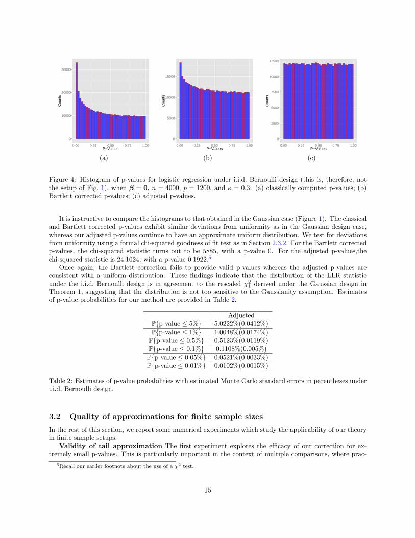
Figure 4: Histogram of p-values for logistic regression under i.i.d. Bernoulli design (this is, therefore, notthe setup of Fig. 1), when β = 0, n = 4000, p = 1200, and κ = 0.3: (a) classically computed p-values; (b)Bartlett corrected p-values; (c) adjusted p-values.

It is instructive to compare the histograms to that obtained in the Gaussian case (Figure 1). The classicaland Bartlett corrected p-values exhibit similar deviations from uniformity as in the Gaussian design case,whereas our adjusted p-values continue to have an approximate uniform distribution. We test for deviationsfrom uniformity using a formal chi-squared goodness of fit test as in Section 2.3.2. For the Bartlett correctedp-values, the chi-squared statistic turns out to be 5885, with a p-value 0. For the adjusted p-values,thechi-squared statistic is 24.1024, with a p-value 0.1922.6

Once again, the Bartlett correction fails to provide valid p-values whereas the adjusted p-values areconsistent with a uniform distribution. These findings indicate that the distribution of the LLR statisticunder the i.i.d. Bernoulli design is in agreement to the rescaled χ2

1 derived under the Gaussian design inTheorem 1, suggesting that the distribution is not too sensitive to the Gaussianity assumption. Estimatesof p-value probabilities for our method are provided in Table 2.

AdjustedPp-value ≤ 5% 5.0222%(0.0412%)Pp-value ≤ 1% 1.0048%(0.0174%)Pp-value ≤ 0.5% 0.5123%(0.0119%)Pp-value ≤ 0.1% 0.1108%(0.005%)Pp-value ≤ 0.05% 0.0521%(0.0033%)Pp-value ≤ 0.01% 0.0102%(0.0015%)

Table 2: Estimates of p-value probabilities with estimated Monte Carlo standard errors in parentheses underi.i.d. Bernoulli design.

3.2 Quality of approximations for finite sample sizesIn the rest of this section, we report some numerical experiments which study the applicability of our theoryin finite sample setups.

Validity of tail approximation The first experiment explores the efficacy of our correction for ex-tremely small p-values. This is particularly important in the context of multiple comparisons, where prac-

6Recall our earlier footnote about the use of a χ2 test.

15

0.0000

0.0025

0.0050

0.0075

0.0100

0.000 0.002 0.004 0.006 0.008 0.010t

Em

piric

al c

df

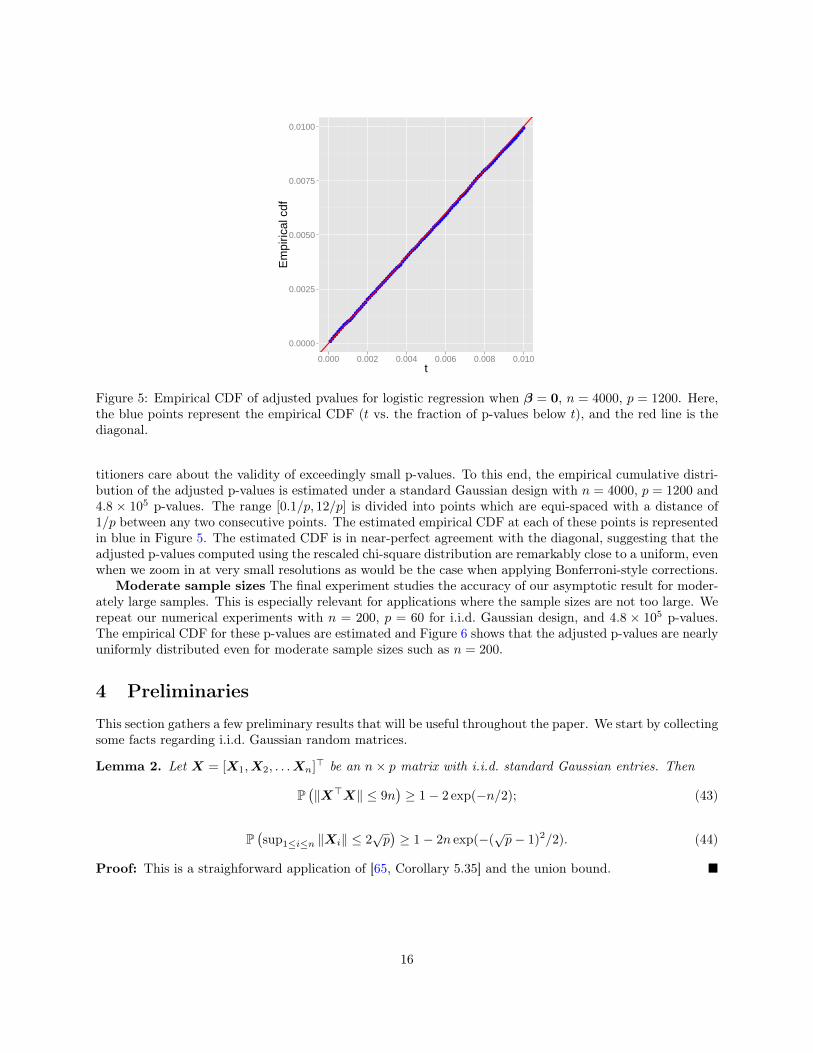
Figure 5: Empirical CDF of adjusted pvalues for logistic regression when β = 0, n = 4000, p = 1200. Here,the blue points represent the empirical CDF (t vs. the fraction of p-values below t), and the red line is thediagonal.

titioners care about the validity of exceedingly small p-values. To this end, the empirical cumulative distri-bution of the adjusted p-values is estimated under a standard Gaussian design with n = 4000, p = 1200 and4.8 × 105 p-values. The range [0.1/p, 12/p] is divided into points which are equi-spaced with a distance of1/p between any two consecutive points. The estimated empirical CDF at each of these points is representedin blue in Figure 5. The estimated CDF is in near-perfect agreement with the diagonal, suggesting that theadjusted p-values computed using the rescaled chi-square distribution are remarkably close to a uniform, evenwhen we zoom in at very small resolutions as would be the case when applying Bonferroni-style corrections.

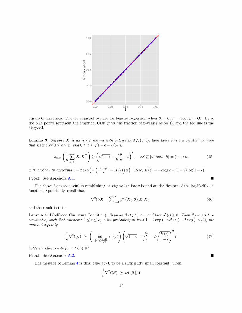
Moderate sample sizes The final experiment studies the accuracy of our asymptotic result for moder-ately large samples. This is especially relevant for applications where the sample sizes are not too large. Werepeat our numerical experiments with n = 200, p = 60 for i.i.d. Gaussian design, and 4.8 × 105 p-values.The empirical CDF for these p-values are estimated and Figure 6 shows that the adjusted p-values are nearlyuniformly distributed even for moderate sample sizes such as n = 200.

4 Preliminaries

This section gathers a few preliminary results that will be useful throughout the paper. We start by collectingsome facts regarding i.i.d. Gaussian random matrices.

Lemma 2. Let X = [X1,X2, . . .Xn]> be an n× p matrix with i.i.d. standard Gaussian entries. Then

P(‖X>X‖ ≤ 9n

)≥ 1− 2 exp(−n/2); (43)

P(sup1≤i≤n ‖Xi‖ ≤ 2

√p)≥ 1− 2n exp(−(

√p− 1)2/2). (44)

Proof: This is a straighforward application of [65, Corollary 5.35] and the union bound.

16

0.00

0.25

0.50

0.75

1.00

0.00 0.25 0.50 0.75 1.00t

Em

piric

al c

df

Figure 6: Empirical CDF of adjusted pvalues for logistic regression when β = 0, n = 200, p = 60. Here,the blue points represent the empirical CDF (t vs. the fraction of p-values below t), and the red line is thediagonal.

Lemma 3. Suppose X is an n × p matrix with entries i.i.d N (0, 1), then there exists a constant ε0 suchthat whenever 0 ≤ ε ≤ ε0 and 0 ≤ t ≤

√1− ε−

√p/n,

λmin

(1

n

∑i∈S

XiX>i

)≥(√

1− ε−√p

n− t)2

, ∀S ⊆ [n] with |S| = (1− ε)n (45)

with probability exceeding 1− 2 exp(−(

(1−ε)t22 −H (ε)

)n). Here, H(ε) = −ε log ε− (1− ε) log(1− ε).

Proof: See Appendix A.1.

The above facts are useful in establishing an eigenvalue lower bound on the Hessian of the log-likelihoodfunction. Specifically, recall that

∇2`(β) =∑n

i=1ρ′′(X>i β

)XiX

>i , (46)

and the result is this:

Lemma 4 (Likelihood Curvature Condition). Suppose that p/n < 1 and that ρ′′(·) ≥ 0. Then there exists aconstant ε0 such that whenever 0 ≤ ε ≤ ε0, with probability at least 1 − 2 exp (−nH (ε)) − 2 exp (−n/2), thematrix inequality

1

n∇2`(β)

(inf

z:|z|≤ 3‖β‖√ε

ρ′′ (z)

)(√

1− ε−√p

n− 2

√H(ε)

1− ε

)2

I (47)

holds simultaneously for all β ∈ Rp.

Proof: See Appendix A.2.

The message of Lemma 4 is this: take ε > 0 to be a sufficiently small constant. Then

1

n∇2`(β) ω(‖β‖) I

17

for some non-increasing, continuous and positive function ω(·) independent of n. This is a generalization ofthe strong convexity condition.

5 When is the MLE bounded?

5.1 Phase transitionIn Section 2.2, we argued that the MLE is at infinity if we have less than two observations per dimension orκ > 1/2. In fact, a stronger version of the phase transition phenemonon occurs in the sense that

‖β‖ = O(1)

as soon as κ < 1/2. This is formalized in the following theorem.

Theorem 4 (Norm Bound Condition). Fix any small constant ε > 0, and let β be the MLE for a modelwith effective link satisfying the conditions from Section 2.3.3.

(i) If p/n ≥ 1/2 + ε, then the MLE does not exist with probability exceeding 1− 4 exp(−ε2n/8

).

(ii) There exist universal constants c1, c2,C2 > 0 such that if p/n < 1/2− c1ε3/4, then7

‖β‖ < 4 log 2

ε2

with probability at least 1− C2 exp(−c2ε2n).

These conclusions clearly continue to hold if β is replaced by β (the MLE under the restricted model obtainedon dropping the first predictor).

The rest of this section is devoted to proving this theorem. As we will see later, the fact that ‖β‖ = O(1)is crucial for utilizing the AMP machinery in the absence of strong convexity.

5.2 Proof of Theorem 4As in Section 2.5.1, we assume yi ≡ 1 throughout this section, and hence the MLE reduces to

minimizeβ∈Rp `0 (β) :=∑n

i=1ρ(−X>i β). (48)

5.2.1 Proof of Part (i)

Invoking [3, Theorem I] yields that if

δ (Xβ | β ∈ Rp) + δ(Rn+)≥ (1 + ε)n,

or equivalently, if p/n ≥ 1/2 + ε, then

PXβ | β ∈ Rp ∩ Rn+ 6= 0

≥ 1− 4 exp

(−ε2n/8

).

As is seen in Section 2.2, ‖β‖ =∞ when Xβ | β ∈ Rp ∩ Rn+ 6= 0, establishing Part (i) of Theorem 4.

7When Xi ∼ N (0,Σ) for a general Σ 0, one has ‖Σ1/2β‖ . 1/ε2 with high probability.

18

5.2.2 Proof of Part (ii)

We now turn to the regime in which p/n ≤ 1/2− O(ε3/4), where 0 < ε < 1 is any fixed constant. Begin byobserving that the least singular value of X obeys

σmin (X) ≥√n/4 (49)

with probability at least 1− 2 exp(− 1

2

(34 −

1√2

)2n)(this follows from Lemma 3 using ε = 0). Then for any

β ∈ Rp obeying`0(β) =

∑n

j=1ρ(−X>j β

)≤ n log 2 = `0(0) (50)

and ‖β‖ ≥ 4 log 2

ε2, (51)

we must haven∑j=1

max−X>j β, 0

=

∑j: X>j β<0

(−X>j β

) (a)

≤∑

j: X>j β<0

ρ(−X>j β

) (b)

≤ n log 2;

(a) follows since t ≤ ρ(t) and (b) is a consequence of (50). Continuing, (49) and (51) give

n log 2 ≤ 4√n‖Xβ‖‖β‖

log 2 ≤ ε2√n‖Xβ‖.

This implies the following proposition: if the solution β—which necessarily satisfies `0(β) ≤ `0(0)—hasnorm exceeding ‖β‖ ≥ 4 log 2

ε2 , then Xβ must fall within the cone

A :=u ∈ Rn

∣∣∣ ∑n

j=1max −uj , 0 ≤ ε2

√n‖u‖

. (52)

Therefore, if one wishes to rule out the possibility of having ‖β‖ ≥ 4 log 2ε2 , it suffices to show that with high

probability,Xβ | β ∈ Rp ∩ A = 0 . (53)

This is the content of the remaining proof.We would like to utilize tools from conic geometry [3] to analyze the probability of the event (53). Note,

however, that A is not convex, while the theory developed in [3] applies only to convex cones. To bypass thenon-convexity issue, we proceed in the following three steps:

1. Generate a set of N = exp(2ε2p

)closed convex cones Bi | 1 ≤ i ≤ N such that it forms a cover of

A with probability exceeding 1− exp(−Ω(ε2p)

).

2. Show that if p <(

12 − 2

√2ε

34 − 2H(2

√ε))n and if n is sufficiently large, then

P Xβ | β ∈ Rp ∩ Bi 6= 0 ≤ 4 exp

−1

8

(1

2− 2√

2ε34 − 10H(2

√ε)− p

n

)2

n

for each 1 ≤ i ≤ N .

3. Invoke the union bound to reach

P Xβ | β ∈ Rp ∩ A 6= 0 ≤ P Bi | 1 ≤ i ≤ N does not form a cover of A

+N∑i=1

P Xβ | β ∈ Rp ∩ Bi 6= 0

≤ exp(−Ω(ε2p)

),

19

where we have used the fact that

N∑i=1

P Xβ | β ∈ Rp ∩ Bi 6= 0 ≤ 4N exp

−1

8

(1

2− 2√

2ε34 − 10H(2

√ε)− p

n

)2

n

< 4 exp

−

(1

8

(1

2− 2√

2ε34 − 10H(2

√ε)− p

n

)2

− 2ε2

)n

< 4 exp

−ε2n

.

Here, the last inequality holds if(

12 − 2

√2ε

34 − 10H(2

√ε)− p

n

)2

> 24ε2, or equivalently, pn < 1

2 −2√

2ε34 − 10H(2

√ε)−

√24ε.

Taken collectively, these steps establish the following claim: if pn <

12 − 2

√2ε

34 − 10H(2

√ε)−

√24ε, then

P‖β‖ > 4 log 2

ε2

< exp

−Ω(ε2n)

,

thus establishing Part (ii) of Theorem 4. We defer the complete details of the preceding steps to AppendixD.

6 Asymptotic `2 error of the MLE

This section aims to establish Theorem 2, which characterizes precisely the asymptotic squared error of theMLE β under the global null β = 0. As described in Section 2.5.1, it suffices to assume that β is the solutionto the following problem

minimizeβ∈Rp∑n

i=1ρ(−X>i β). (54)

In what follows, we derive the asymptotic convergence of ‖β‖ under the assumptions from our main theorem.

Theorem 5. Under the assumptions of Theorem 1, the solution β to (54) obeys

limn→∞

‖β‖2 =a.s. τ2∗ . (55)

Theorem 5 is derived by invoking the AMP machinery [7, 8, 38]. The high-level idea is the following:in order to study β, one introduces an iterative algorithm (called AMP) where a sequence of iterates βt isformed at each time t. The algorithm is constructed so that the iterates asymptotically converge to the MLEin the sense that

limt→∞

limn→∞

‖βt − β‖2 =a.s. 0. (56)

On the other hand, the asymptotic behavior (asymptotic in n) of βt for each t can be described accuratelyby a scalar sequence τt—called state evolution (SE)—following certain update equations [7]. This, in turn,provides a characterization of the `2 loss of β.

Further, in order to prove Theorem 2, one still needs to justify

(a) the existence of a solution to the system of equations (25) and (26),

(b) and the existence of a fixed point for the iterative map governing the SE sequence updates.

We will elaborate on these steps in the rest of this section.

20

6.1 State evolutionWe begin with the SE sequence τt introduced in [22]. Starting from some initial point τ0, we produce twosequences bt and τt following a two-step procedure.

• For t = 0, 1, . . .:

– Set bt to be the solution in b to

κ = E[Ψ′(τtZ; b)

]; (57)

– Set τt+1 to be

τ2t+1 =

1

κE[(Ψ2(τtZ; bt))

]. (58)

Suppose that for given any τ > 0, the solution in b to (57) with τt = τ exists and is unique, then one candenote the solution as b(τ), which in turn allows one to write the sequence τt as

τ2t+1 = V(τ2

t )

with the variance map

V(τ2) =1

κE[Ψ2(τZ; b(τ))

]. (59)

As a result, if there exists a fixed point τ∗ obeying V(τ2∗ ) = τ2

∗ and if we start with τ0 = τ∗, then by induction,

τt ≡ τ∗ and bt ≡ b∗ := b(τ∗), t = 0, 1, . . .

Notably, (τ∗, b∗) solves the system of equations (25) and (26). We shall work with this choice of initialcondition throughout our proof.

The preceding arguments hold under two conditions: (i) the solution to (57) exists and is unique forany τt > 0; (ii) the variance map (59) admits a fixed point. To verify these two conditions, we make twoobservations.

• Condition (i) holds if one can show that the function

G(b) := E [Ψ′(τZ; b)] , b > 0 (60)

is strictly monotone for any given τ > 0, and that limb→0G(b) < κ < limb→∞G(b).

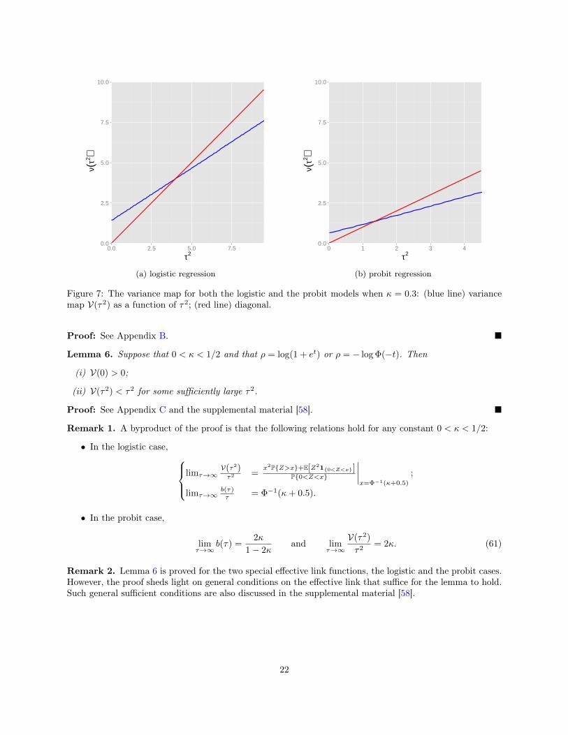
• Since V(·) is a continuous function, Condition (ii) becomes self-evident once we show that V(0) > 0and that there exists τ > 0 obeying V(τ2) < τ2. The behavior of the variance map is illustrated inFigure 7 for the logistic and probit regression when κ = 0.3. One can in fact observe that the fixedpoint is unique. For other values of κ, the variance map shows the same behavior.

In fact, the aforementioned properties can be proved for a certain class of effective links, as summarizedin the following lemmas. In particular, they can be shown for the logistic and the probit models.

Lemma 5. Suppose the effective link ρ satisfies the following two properties:

(a) ρ′ is log-concave.

(b) For any fixed τ > 0 and any fixed z, bρ′′(proxbρ(τz))→∞ when b→∞.

Then for any τ > 0, the function G(b) defined in (60) is an increasing function in b (b > 0), and the equation

G(b) = κ

has a unique positive solution.

21

0.0

2.5

5.0

7.5

10.0

0.0 2.5 5.0 7.5

τ2

ν(τ2 )

(a) logistic regression

0.0

2.5

5.0

7.5

10.0

0 1 2 3 4

τ2

ν(τ2 )

(b) probit regression

Figure 7: The variance map for both the logistic and the probit models when κ = 0.3: (blue line) variancemap V(τ2) as a function of τ2; (red line) diagonal.

Proof: See Appendix B.

Lemma 6. Suppose that 0 < κ < 1/2 and that ρ = log(1 + et) or ρ = − log Φ(−t). Then

(i) V(0) > 0;

(ii) V(τ2) < τ2 for some sufficiently large τ2.

Proof: See Appendix C and the supplemental material [58].

Remark 1. A byproduct of the proof is that the following relations hold for any constant 0 < κ < 1/2:

• In the logistic case, limτ→∞V(τ2)τ2 =

x2PZ>x+E[Z210<Z<x]P0<Z<x

∣∣∣∣x=Φ−1(κ+0.5)

;

limτ→∞b(τ)τ = Φ−1(κ+ 0.5).

• In the probit case,

limτ→∞

b(τ) =2κ

1− 2κand lim

τ→∞

V(τ2)

τ2= 2κ. (61)

Remark 2. Lemma 6 is proved for the two special effective link functions, the logistic and the probit cases.However, the proof sheds light on general conditions on the effective link that suffice for the lemma to hold.Such general sufficient conditions are also discussed in the supplemental material [58].

22

6.2 AMP recursion

In this section, we construct the AMP trajectory tracked by two sequences βt(n) ∈ Rp and ηt(n) ∈ Rnfor t ≥ 0. Going forward we suppress the dependence on n to simplify presentation. Picking β0 such that

limn→∞

‖β0‖2 = τ20 = τ2

∗

and taking η−1 = 0 and b−1 = 0, the AMP path is obtained via Algorithm 1, which is adapted from thealgorithm in [22, Section 2.2].

Algorithm 1 Approximate message passing.For t = 0, 1, · · · :

1. Setηt = Xβt + Ψ

(ηt−1; bt−1

); (62)

2. Let bt be the solution toκ = E [Ψ′(τtZ; b)] , (63)

where τt is the SE sequence value at that time.

3. Setβt+1 = βt − 1

pX>Ψ

(ηt; bt

). (64)

Here, Ψ(·) is applied in an entrywise manner, and Ψ′(., .) denotes derivative w.r.t the first variable.

As asserted by [22], the SE sequence τt introduced in Section 6.1 proves useful as it offers a formalprocedure for predicting operating characteristics of the AMP iterates at any fixed iteration. In particularit assigns predictions to two types of observables: observables which are functions of the βt sequence andthose which are functions of ηt. Repeating identical argument as in [22, Theorem 3.4], we obtain

limn→∞

‖βt‖2 =a.s. τ2t ≡ τ2

∗ , t = 0, 1, . . . . (65)

6.3 AMP converges to the MLE

We are now in position to show that the AMP iterates βt converge to the MLE in the large n and t limit.Before continuing, we state below two properties that are satisfied under our assumptions.

• The MLE β obeyslimn→∞

‖β‖ <∞ (66)

almost surely.

• And there exists some non-increasing continuous function 0 < ω (·) < 1 independent of n such that

P

1

n∇2` (β) ω (‖β‖) · I, ∀β

≥ 1− c1e−c2n. (67)

In fact, the norm bound (66) follows from Theorem 4 together with Borel-Cantelli, while the likelihoodcurvature condition (67) is an immediate consequence of Lemma 4. With this in place, we have:

Theorem 6. Suppose (66) and (67) hold. Let (τ∗, b∗) be a solution to the system (25) and (26), and assumethat limn→∞ ‖β0‖2 = τ2

∗ . Then the AMP trajectory as defined in Algorithm 1 obeys

limt→∞

limn→∞

‖βt − β‖ =a.s. 0.

23

Taken collectively, Theorem 6 and Eqn. (65) imply that

limn→∞

‖β‖ =a.s. limt→∞

limn→∞

‖βt‖ =a.s. τ∗, (68)

thus establishing Theorem 5. In addition, an upshot of these theorems is a uniqueness result:

Corollary 2. The solution to the system of equations (25) and (26) is unique.

Proof: When the AMP trajectory βt is started with the initial condition from Theorem 6, limn→∞ ‖β‖2 =a.s.τ2∗ . This holds for any τ∗ such that (τ∗, b∗) is a solution to (25) and (26). However, since the MLE problemis strongly convex and hence admits a unique solution β, this implies that τ∗ must be unique, which togetherwith the monotonicity of G(·) (cf. (60)) implies that b∗ is unique as well.

Proof of Theorem 6: To begin with, repeating the arguments in [22, Lemma 6.9] we reach

limt→∞

limn→∞

‖βt+1 − βt‖2 =a.s. 0; (69)

limt→∞

limn→∞

1

n‖ηt+1 − ηt‖2 =a.s. 0. (70)

To show that the AMP iterates converge to the MLE, we shall analyze the log-likelihood function. Recallfrom Taylor’s theorem that

`(β) = `(βt) +⟨∇`(βt), β − βt

⟩+

1

2

(β − βt

)>∇2`

(βt + λ(β − βt)

)(β − βt

)holds for some 0 < λ < 1. To deal with the quadratic term, we would like to control the Hessian of thelikelihood at a point between β and βt. Invoking the likelihood curvature condition (67), one has

`(βt) ≥ `(β) ≥ `(βt) +⟨∇`(βt), β − βt

⟩+

1

2nω(

max‖β‖, ‖βt‖

)‖β − βt‖2 (71)

with high probability. Apply Cauchy-Schwarz to yield that with exponentially high probability,

‖β − βt‖ ≤ 2

ω(

max‖β‖, ‖βt‖

)∥∥∥ 1

n∇`(βt)

∥∥∥ ≤ 2

ω(‖β‖

)ω(‖βt‖

)∥∥∥ 1

n∇`(βt)

∥∥∥,

where the last inequality follows since 0 < ω(·) < 1 and ω(·) is non-increasing.It remains to control ‖∇`(βt)‖. The identity Ψ(z; b∗) = z − proxb∗ρ(z) and (62) give

proxb∗ρ(ηt−1

)= Xβt + ηt−1 − ηt. (72)

In addition, substituting Ψ (z; b) = bρ′(proxρb(z)) into (64) yields

p

b∗(βt − βt−1) = −X>ρ′

(proxb∗ρ(η

t−1))

= −X>ρ′(Xβt + ηt−1 − ηt

).

We are now ready to bound ‖∇`(βt)‖. Recalling that

∇`(βt) = X>ρ′(X>βt) = X>ρ′(Xβt + ηt−1 − ηt

)+X>

(ρ′(X>βt)− ρ′

(Xβt + ηt−1 − ηt

))and that supz ρ

′′(z) <∞, we have∥∥∇`(βt)∥∥ ≤∥∥∥−X>ρ′ (Xβt + ηt−1 − ηt

)∥∥∥+ ‖X‖∣∣∣ρ′ (Xβt + ηt−1 − ηt

)− ρ′(Xβt)

∣∣∣≤ p

b∗‖βt − βt−1‖+ ‖X‖

(supzρ′′(z)

)‖ηt−1 − ηt‖.

24

This establishes that with probability at least 1− c1e−c2n,

‖β − βt‖ ≤ 2

ω(‖β‖

)ω(‖βt‖

) p

b∗n‖βt − βt−1‖+

1

n

(supzρ′′(z)

)‖X‖‖ηt−1 − ηt‖

. (73)

Using (44) together with Borel-Cantelli yields limn→∞ ‖X‖/√n < ∞ almost surely. Further, it follows

from (65) that limn→∞ ‖βt‖ is finite almost surely as τ∗ <∞. These taken together with (66), (69) and (70)yield

limt→∞

limn→∞

‖β − βt‖ =a.s. 0 (74)

as claimed.

7 Likelihood ratio analysis

This section presents the analytical details for Section 2.5.2, which relates the log-likelihood ratio statisticΛi with βi. Recall from (37) that the LLR statistic for testing β1 = 0 vs. β1 6= 0 is given by

Λ1 =1

2

(Xβ −Xβ

)>Dβ

(Xβ −Xβ

)+

1

6

n∑i=1

ρ′′′(γi)(X>i β −X>i β

)3

, (75)

where

Dβ :=

ρ′′(X>1 β

). . .

ρ′′(X>n β

) (76)

and γi lies between X>i β and X>i β. The asymptotic distribution of Λ1 claimed in Theorem 3 immediatelyfollows from the result below, whose proof is the subject of the rest of this section.

Theorem 7. Let (τ∗, b∗) be the unique solution to the system of equations (25) and (26), and define

G =1

nX>DβX and α =

1

nTr(G−1). (77)

Suppose p/n→ κ ∈ (0, 1/2) . Then

(a) the log-likelihood ratio statistic obeys

2Λ1 − pβ21/α

P→ 0; (78)

(b) and the scalar α converges,α

P→ b∗. (79)

7.1 More notations and preliminariesBefore proceeding, we introduce some notations that will be used throughout. For any matrix X, denoteby Xij and X·j its (i, j)-th entry and jth column, respectively. We denote an analogue r = ri1≤i≤n(resp. r = ri1≤i≤n) of residuals in the full (resp. reduced) model by

ri := −ρ′(X>i β

)and ri := −ρ′

(X>i β

). (80)

25

As in (76), set

Dβ :=

ρ′′(X>1 β

). . .

ρ′′(X>n β

) and Dβ,b :=

ρ′′ (γ∗1). . .

ρ′′(γ∗n),

, (81)

where γ∗i is betweenX>i β andX>i b, and b is to be defined later in Section 7.2. Further, as in (77), introducethe Gram matrices

G :=1

nX>DβX and Gβ,b =

1

nX>Dβ,bX. (82)

Let G(i) denote the version of G without the term corresponding to the ith observation, that is,

G(i) =1

n

∑j:j 6=i

ρ′′(X>j β)XjX>j . (83)

Additionally, let β[−i] be the MLE when the ith observation is dropped and let G[−i] be the correspondingGram matrix,

G[−i] =1

n

∑j:j 6=i

ρ′′(X>j β[−i])XjX>j . (84)

Further, let β[−i] be the MLE when the first predictor and ith observation are removed, i.e.

β[−i] := arg minβ∈Rp−1

∑j:j 6=i

ρ(X>j β).

Below G[−i] is the corresponding version of G,

G[−i] =1

n

∑j:j 6=i

ρ′′(X>j β[−i])XjX>j . (85)

For these different versions of G, their least eigenvalues are all bounded away from 0, as asserted by thefollowing lemma.

Lemma 7. There exist some absolute constants λlb,C, c > 0 such that

P(λmin(G) > λlb) ≥ 1− Ce−cn.

Moreover, the same result holds for G, Gβ,b, G(i), G[−i] and G[−i] for all i ∈ [n].

Proof: This result follows directly from Lemma 2, Lemma 4, and Theorem 4.

Throughout the rest of this section, we restrict ourselves (for any given n) to the following event:

An := λmin(G) > λlb ∩ λmin(G) > λlb ∩ λmin(Gβ,b) > λlb

∩ ∩ni=1λmin(G(i)) > λlb ∩ ∩ni=1λmin(G[−i]) > λlb ∩ ∩ni=1λmin(G[−i]) > λlb. (86)

By Lemma 7, An arises with exponentially high probability, i.e.

P(An) ≥ 1− exp(−Ω(n)). (87)

26

7.2 A surrogate for the MLE

In view of (75), the main step in controlling Λ1 consists of characterizing the differences Xβ − Xβ or

β −[

0

β

]. Since the definition of β is implicit and not amenable to direct analysis, we approximate β by

a more amenable surrogate b, an idea introduced in [24–26]. We collect some properties of the surrogatewhich will prove valuable in the subsequent analysis.

To begin with, our surrogate is

b =

[0

β

]+ b1

[1

−G−1w

], (88)

where G is defined in (82),

w :=1

n

∑n

i=1ρ′′(X>i β)Xi1Xi =

1

nX>DβX·1, (89)

and b1 is a scalar to be specified later. This vector is constructed in the hope that

β ≈ b, or equivalently,

β1 ≈ b1,

β2:p − β ≈ −b1G−1w,(90)

where β2:p contains the 2nd through pth components of β.Before specifying b1, we shall first shed some insights into the remaining terms in b. By definition,

∇2`

([0

β

])= X>DβX =

[X>·1DβX·1 X>·1DβX

X>DβX·1 X>DβX

]=

[X>·1DβX·1 nw>

nw nG

].

Employing the first-order approximation of ∇`(·) gives

∇2`

([0

β

])(β −

[0

β

])≈ ∇`(β)−∇`

([0

β

]). (91)

Suppose β2:p is well approximated by β. Then all but the first coordinates of ∇`(β) and ∇`([

0

β

])are

also very close to each other. Therefore, taking the 2nd through pth components of (91) and approximatingthem by zero give [

w, G](β −

[0

β

])≈ 0.

This together with a little algebra yields

β2:p − β ≈ −β1G−1w ≈ −b1G−1w,

which coincides with (90). In fact, for all but the 1st entries, b is constructed by moving β one-step in thedirection which takes it closest to β.

Next, we come to discussing the scalar b1. Introduce the projection matrix

H := I − 1

nD

1/2

βXG−1X>D

1/2

β, (92)

and define b1 as

b1 :=X>·1 r

X>·1D1/2

βHD

1/2

βX·1

, (93)

27

where r comes from (80). In fact, the expression b1 is obtained through similar (but slightly more compli-cated) first-order approximation as for b2:p, in order to make sure that b1 ≈ β1; see [26, Pages 14560-14561]for a detailed description.

We now formally justify that the surrogate b and the MLE β are close to each other.

Theorem 8. The MLE β and the surrote b (88) obey

‖β − b‖ . n−1+o(1), (94)

|b1| . n−1/2+o(1), (95)

andsup

1≤i≤n|X>i b− X>i β| . n−1/2+o(1) (96)

with probability tending to one as n→∞.

Proof: See Section 7.4.

The global accuracy (94) immediately leads to a coordinate-wise approximation result between β1 andb1.

Corollary 3. With probability tending to one as n→∞,√n|b1 − β1| . n−1/2+o(1). (97)

Another consequence from Theorem 8 is that the value X>i β in the full model and its counterpart X>i βin the reduced model are uniformly close.

Corollary 4. The values X>i β and X>i β are uniformly close in the sense that

sup1≤i≤n

∣∣X>i β − X>i β∣∣ . n−1/2+o(1) (98)

holds with probability approaching one as n→∞.

Proof: Note that

sup1≤i≤n

∣∣X>i β − X>i β∣∣ ≤ sup1≤i≤n

∣∣X>i (β − b)∣∣+ sup

1≤i≤n

∣∣X>i b− X>i β∣∣.The second term in the right-hand side is upper bounded by n−1/2+o(1) with probability 1− o(1) accordingto Theorem 8. Invoking Lemma 2 and Theorem 8 and applying Cauchy-Schwarz inequality yield that thefirst term is O(n−1/2+o(1)) with probability 1− o(1). This establishes the claim.

7.3 Analysis of the likelihood-ratio statistic

We are now positioned to use our surrogate b to analyze the likelihood-ratio statistic. In this subsection weestablish Theorem 7(a). The proof for Theorem 7(b) is deferred to Appendix I.

Recall from (37) that

2Λ1 = (Xβ −Xβ)>Dβ(Xβ −Xβ) +1

3

n∑i=1

ρ′′′(γi)(X>i β −X>i β)3

︸ ︷︷ ︸:=I3

.

28

To begin with, Corollary 4 together with the assumption supz ρ′′′(z) <∞ implies that

I3 . n−1/2+o(1)

with probability 1− o(1). Hence, I3 converges to zero in probability.Reorganize the quadratic term as follows:

(Xβ −Xβ)>Dβ(Xβ −Xβ) =∑i

ρ′′(X>i β)(X>i β − X>i β

)2

=∑i

ρ′′(X>i β)[X>i (β − b) + (X>i b− X>i β)

]2=∑i

ρ′′(X>i β)(X>i (β − b))2 + 2∑i

ρ′′(X>i β)X>i (β − b)(X>i b− X>i β)

+∑i

ρ′′(X>i β)(X>i b− X>i β

)2. (99)

We control each of the three terms in the right-hand side of (99).

• Since supz ρ′′(z) <∞, the first term in (99) is bounded by∑

iρ′′(X>i β)(X>i (β − b))2 . ||β − b||2

∥∥∥∑iXiX

>i

∥∥∥ . n−1+o(1)

with probability 1− o(1), by an application of Theorem 8 and Lemma 2.

• From the definition of b, the second term can be upper bounded by

2∑i

ρ′′(X>i β)(β − b)>XiX>i b1

[1

−G−1w

]≤ |b1| · ‖β − b‖ ·

∥∥∥∑iXiX

>i

∥∥∥ ·√1 +w>G−2w

. n−12 +o(1)

with probability 1− o(1), where the last line follows from a combination of Theorem 8, Lemma 2 andthe following lemma.

Lemma 8. Let G and w be as defined in (82) and (89), respectively. Then

P(w>G−2w . 1

)≥ 1− exp(−Ω(n)). (100)

Proof: See Appendix E.

• The third term in (99) can be decomposed as∑i

ρ′′(X>i β)(X>i b− X>i β))2

=∑i

(ρ′′(X>i β)− ρ′′(X>i β)

)(X>i b− X>i β))2 +

∑i

ρ′′(X>i β)(X>i b− X>i β)2

=∑i

ρ′′′(γi)(X>i β − X>i β)

(X>i b− X>i β

)2

+∑i

ρ′′(X>i β)(X>i b− X>i β

)2

(101)

for some γi between X>i β and X>i β. From Theorem 8 and Corollary 4, the first term in (101) isO(n−1/2+o(1)) with probability 1− o(1). Hence, the only remaining term is the second.

29

In summary, we have

2Λ1 −∑i

ρ′′(X>i β)(X>i b− X>i β

)2

︸ ︷︷ ︸=v>X>DβXv

P→ 0, (102)

where v := b1

[1

−G−1w

]according to (88). On simplification, the quadratic form reduces to

v>X>DβXv = b21

(X·1 − XG−1w

)>Dβ

(X·1 − XG−1w

)= b21

(X>·1DβX·1 − 2X>·1DβXG

−1w +w>G−1X>DβXG−1w

)= b21

(X>·1DβX·1 − nw

>G−1w)

= nb21

(1

nX>·1D

1/2

βHD

1/2

βX·1︸ ︷︷ ︸

:=ξ

),

recalling the definitions (82), (89), and (92). Hence, the log-likelihood ratio 2Λ1 simplifies to nb21ξ + oP (1)on An.

Finally, rewrite v>X>DβXv as n(b21 − β21)ξ + nβ2

1ξ. To analyze the first term, note that

n|b21 − β21 | = n|b1 − β1| · |b1 + β1| ≤ n|b1 − β1|2 + 2n|b1| · |b1 − β1| . n−

12 +o(1) (103)

with probability 1− o(1) in view of Theorem 8 and Corollary 3. It remains to analyze ξ. Recognize that X·1is independent of D1/2

βHD

1/2

β. Applying the Hanson-Wright inequality [32,52] and the Sherman-Morrison-

Woodbury formula (e.g. [31]) leads to the following lemma:

Lemma 9. Let α = 1nTr(G−1), where G = 1

nX>DβX. Then one has∣∣∣∣p− 1

n− α 1

nX>·1D

1/2

βHD

1/2

βX·1

∣∣∣∣ . n−1/2+o(1) (104)

with probability approaching one as n→∞.

Proof: See Appendix F.

In addition, if one can show that α is bounded away from zero with probability 1− o(1), then it is seen fromLemma 9 that

ξ − p

nα

P→ 0. (105)

To justify the above claim, we observe that since ρ′′ is bounded, λmax(G) . λmax(X>X)/n . 1 withexponentially high probability (Lemma 2). This yields

α = Tr(G−1)/n & p/n

with probability 1− o(1). On the other hand, on An one has

α ≤ p/(nλmin(G)) . p/n.

Hence, it follows that ξ = Ω(1) with probability 1 − o(1). Putting this together with (103) gives theapproximation

v>X>DβXv = nβ21ξ + o(1). (106)

Taken collectively (102), (105) and (106) yields the desired result

2Λ1 − pβ21/α

P→ 0.

30

7.4 Proof of Theorem 8This subsection outlines the main steps for the proof of Theorem 8. To begin with, we shall express thedifference β − b in terms of the gradient of the negative log-likelihood function. Note that ∇`(β) = 0, andhence

∇`(b) = ∇`(b)−∇`(β) =∑n

i=1Xi[ρ

′(X>i b)− ρ′(X ′iβ)]

=∑n

i=1ρ′′(γ∗i )XiX

>i (b− β),

where γ∗i is between X>i β and X>i b. Recalling the notation introduced in (82), this can be rearranged as

b− β =1

nG−1

β,b∇`(b).

Hence, on An, this yields

‖β − b‖ ≤ ‖∇`(b)‖λlbn

. (107)

The next step involves expressing ∇`(b) in terms of the difference b−[

0

β

].

Lemma 10. On the event An (86), the negative log-likelihood evaluated at the surrogate b obeys

∇`(b) =

n∑i=1

[ρ′′(γ∗i )− ρ′′(X>i β)

]XiX

>i

(b−

[0

β

]),

where γ∗i is some quantity between X>i b and X>i β.

Proof: The proof follows exactly the same argument as in the proof of [25, Proposition 3.11], and is thusomitted.

The point of expressing ∇`(b) in this way is that the difference b −[

0

β

]is known explicitly from the

definition of b. Invoking Lemma 10 and the definition (88) allows one to further upper bound (107) as

‖β − b‖ . 1

n

∥∥∥∇`(b)∥∥∥ . supi

∣∣∣ρ′′(γ∗i )− ρ′′(X>i β)∣∣∣ ∥∥∥∥∥ 1

n

n∑i=1

XiX>i

∥∥∥∥∥∥∥∥∥b− [ 0

β

]∥∥∥∥. sup

i

∣∣∣X>i b− X>i β∣∣∣ |ρ′′′|∞ ∥∥∥∥ 1

n

∑n

i=1XiX

>i

∥∥∥∥ · |b1|√1 +w>G−2w

. |b1| supi

∣∣∣X>i b− X>i β∣∣∣ (108)

with probability at least 1 − exp(−Ω(n)). The last inequality here comes from our assumption thatsupz |ρ′′′(z)| <∞ together with Lemmas 2 and 8.

In order to bound (108), we first make use of the definition of b to reach

supi

∣∣∣X>i b− X>i β∣∣∣ = |b1| supi|Xi1 − X>i G−1w|. (109)

The following lemma provides an upper bound on supi |Xi1 − X>i G−1w|.

Lemma 11. With G and w as defined in (82) and (89),

P(

sup1≤i≤n

∣∣Xi1 − X>i G−1w∣∣ ≤ no(1)

)≥ 1− o(1). (110)

31

Proof: See Appendix G.

In view of Lemma 11, the second term in the right-hand side of (109) is bounded above by no(1) withhigh probability. Thus, in both the bounds (108) and (109), it only remains to analyze the term b1. To thisend, we control the numerator and the denominator of b1 separately.

• Recall from the definition (93) that the numerator of b1 is given by X>·1 r and that r is independentof X·1. Thus, conditional on X, the quantity X>·1 r is distributed as a Gaussian with mean zero andvariance

σ2 =∑n

i=1

(ρ′(X>i β)

)2.

Since |ρ′(x)| = O(|x|), the variance is bounded by

σ2 . β>(∑n

i=1XiX

>i

)β . n‖β‖2 . n (111)

with probability at least 1 − exp(−Ω(n))), a consequence from Theorem 4 and Lemma 2. Therefore,with probability 1− o(1), we have

1√nX>·1 r . no(1). (112)

• We now move on to the denominator of b1 in (93). In the discussion following Lemma 9 we showed1nX

>·1D

1/2

βHD

1/2

βX·1 = Ω(1) with probability 1− o(1).

Putting the above bounds together, we conclude

P(|b1| . n−

12 +o(1)

)= 1− o(1). (113)

Substitution into (108) and (109) yields

‖β − b‖ . n−1+o(1) and supi

∣∣∣X>i b− X>i β∣∣∣ . n−1/2+o(1)

with probability 1− o(1) as claimed.

8 Discussion

In this paper, we derived the high-dimensional asymptotic distribution of the LLR under our modellingassumptions. In particular, we showed that the LLR is inflated vis a vis the classical Wilks’ approximationand that this inflation grows as the dimensionality κ increases. This inflation is typical of high-dimensionalproblems, and one immediate practical consequence is that it explains why classically computed p-values arecompletely off since they tend to be far too small under the null hypothesis. In contrast, we have shownin our simulations that our new limiting distribution yields reasonably accurate p-values in finite samples.Having said this, our work raises a few important questions that we have not answered and we conclude thispaper with a couple of them.

• We expect that our results continue to hold when the covariates are not normally distributed; seeSection 3 for some numerical evidence in this direction. To be more precise, we expect the samelimiting distribution to hold when the variables are simply sub-Gaussian so that our approximationwould enjoy a form of universal validity. Notably, all three sets of analysis techniques we employ inthis work have already been extended to accommodate non-Gaussian designs for other problems: theuniversality law of several convex geometry results has been established via the Lindeberg principle [46];the AMP machinery has been extended to non-Gaussian designs via the moment method (e.g. [6,21]);and the leave-one-out analysis developed can readily cope with other types of i.i.d. random designs aswell [25]. Taken collectively, these suggest a possible path to establish the universality of our results.

32

• A major limitation of our work is the fact that our limiting distribution holds under the global null; thatis, under the assumption that all the regression coefficients vanish. A natural question is, therefore,how would the distribution change in the case where the coefficients are not all zero? Consider forinstance the setup where the empirical distribution of the regression coefficients satisfies

1

p

p∑i=1

δβid→ Π,

where Π is some limiting distribution. How is the distribution of LLR affected by Π? While thismanuscript was under review, the first and third authors have established, among other results, anexplicit characterization for the existence of the MLE and the limiting distribution of the LRT in thissetup [57]. The proofs in this manuscript are the foundation of this follow-up work, although severalnew ideas are needed. We refer the interested reader to [56] for an in-depth explanation. In sum, theinsights from this paper are essential for establishing a complete likelihood theory.

Acknowledgements

E. C. was partially supported by the Office of Naval Research under grant N00014-16-1-2712, and by theMath + X Award from the Simons Foundation. P. S. was partially supported by the Ric Weiland GraduateFellowship in the School of Humanities and Sciences, Stanford University. Y. C. is supported in part by theAFOSR YIP award FA9550-19-1-0030, by the ARO grant W911NF-18-1-0303, and by the Princeton SEASinnovation award. P. S. and Y. C. are grateful to Andrea Montanari for his help in understanding AMPand [22]. Y. C. thanks Kaizheng Wang and Cong Ma for helpful discussion about [25], and P. S. thanksSubhabrata Sen for several helpful discussions regarding this project. E. C. would like to thank Iain Johnstonefor a helpful discussion as well.

A Proofs for Eigenvalue Bounds

A.1 Proof of Lemma 3

Fix ε ≥ 0 sufficiently small. For any given S ⊆ [n] obeying |S| = (1 − ε)n and 0 ≤ t ≤√

1− ε −√p/n it

follows from [65, Corollary 5.35] that

λmin

(1

n

∑i∈S

XiX>i

)<

1

n

(√|S| − √p− t

√n)2

=

(√1− ε−

√p

n− t)2

holds with probability at most 2 exp(− t

2|S|2

)= 2 exp

(− (1−ε)t2n

2

). Taking the union bound over all possible

subsets S of size (1− ε)n gives

P

∃S ⊆ [n] with |S| = (1− ε)n s.t.

1

nλmin

(∑i∈S

XiX>i

)<

(√1− ε−

√p

n− t)2

≤(

n

(1− ε)n

)2 exp

(− (1− ε) t2n

2

)≤ 2 exp

(nH (ε)− (1− ε) t2

2n

),

where the last line is a consequence of the inequality(

n(1−ε)n

)≤ enH(ε) [19, Example 11.1.3].

33

A.2 Proof of Lemma 4Define

SB (β) :=i : |X>i β| ≤ B‖β‖

for any B > 0 and any β. Then

n∑i=1

ρ′′(X>i β

)XiX

>i

∑i∈SB(β)

ρ′′(X>i β

)XiX

>i inf

z:|z|≤B‖β‖ρ′′ (z)

∑i∈SB(β)

XiX>i .

If one also has |SB (β) | ≥ (1 − ε)n (for ε ≥ 0 sufficiently small), then this together with Lemma 3 impliesthat

1

n

n∑i=1

ρ′′(X>i β

)XiX

>i inf

z:|z|≤B‖β‖ρ′′ (z)

(√1− ε−

√p

n− t)2

I

with probability at least 1− 2 exp(−(

(1−ε)t22 −H (ε)

)n).

Thus if we can ensure that with high probability, |SB (β) | ≥ (1− ε)n holds simultaneously for all β, thenwe are done. From Lemma 2 we see that 1

n

∥∥X>X∥∥ ≤ 9 with probability exceeding 1 − 2 exp (−n/2). Onthis event,

‖Xβ‖2 ≤ 9n‖β‖2, ∀β. (114)On the other hand, the definition of SB(β) gives

‖Xβ‖2 ≥∑

i/∈SB(β)

∣∣X>i β∣∣2 ≥ (n− |SB(β)|)

(B‖β‖)2= n

(1− |SB(β)|

n

)B2‖β‖2. (115)

Taken together, (114) and (115) yield

|SB(β)| ≥(

1− 9

B2

)n, ∀β

with probability at least 1−2 exp(−n/2). Therefore, with probability 1−2 exp(−n/2),∣∣S3/

√ε(β)

∣∣ ≥ (1− ε)n

holds simultaneously for all β. Putting the above results together and setting t = 2√

H(ε)1−ε give

n∑i=1

ρ′′(X>i β

)XiX

>i inf

z:|z|≤ 3‖β‖√ε

ρ′′ (z)

(√

1− ε−√p

n− 2

√H(ε)

1− ε

)2

I

simultaneously for all β with probability at least 1− 2 exp (−nH (ε))− 2 exp (−n/2).

B Proof of Lemma 5

Applying an integration by parts leads to

E [Ψ′(τZ; b)] =

∫ ∞−∞

Ψ′(τz; b)φ(z)dz =1

τΨ(τz; b)φ(z)

∣∣∣∞−∞− 1

τ

∫ ∞−∞

Ψ(τz; b)φ′(z)dz

= −1

τ

∫ ∞−∞

Ψ(τz; b)φ′(z)dz

with φ(z) = 1√2π

exp(−z2/2). This reveals that

G′(b) = −1

τ

∫ ∞−∞

∂Ψ(τz; b)

∂bφ′(z)dz = −1

τ

∫ ∞−∞

ρ′(proxbρ(τz)

)1 + bρ′′

(proxbρ(τz)

)φ′(z)dz=

1

τ

∫ ∞0

(ρ′(proxbρ(−τz)

)1 + xρ′′

(proxbρ(−τz)

) − ρ′(proxbρ(τz)

)1 + xρ′′

(proxbρ(τz)

))φ′(z)dz, (116)

34

where the second identity comes from [22, Proposition 6.4], and the last identity holds since φ′(z) = −φ′(−z).Next, we claim that

(a) The function h (z) := ρ′(z)1+bρ′′(z) is increasing in z;

(b) proxbρ(z) is increasing in z.

These two claims imply that

ρ′(proxbρ(−τz)

)1 + bρ′′

(proxbρ(−τz)

) − ρ′(proxbρ(τz)

)1 + bρ′′

(proxbρ(τz)

) < 0, ∀z > 0,

which combined with the fact φ′(z) < 0 for z > 0 reveals

sign

((ρ′(proxbρ(−τz)

)1 + bρ′′

(proxbρ(−τz)

) − ρ′(proxbρ(τz)

)1 + bρ′′

(proxbρ(τz)

))φ′(z)) = 1, ∀z > 0.

In other words, the integrand in (116) is positive, which allows one to conclude that G′(b) > 0.We then move on to justify (a) and (b). For the first, the derivative of h is given by

h′(z) =ρ′′(z) + b(ρ′′(z))2 − bρ′(z)ρ′′′(z)

(1 + bρ′′(z))2 .

Since ρ′ is log concave, this directly yields (ρ′′)2−ρ′ρ′′′ > 0. As ρ′′ > 0 and b ≥ 0, the above implies h′(z) > 0

for all z. The second claim follows from ∂proxbρ(z)

∂z ≥ 11+b‖ρ′′‖∞ > 0 (cf. [22, Equation (56)]).

It remains to analyze the behavior of G in the limits when b→ 0 and b→∞. From [22, Proposition 6.4],G(b) can also be expressed as

G(b) = 1− E[

1

1 + bρ′′(proxbρ(τZ))

].

Since ρ′′ is bounded and the integrand is at most 1, the dominated convergence theorem gives

limb→0

G(b) = 0.

When b→∞, bρ′′(proxbρ(τz))→∞ for a fixed z. Again by applying the dominated convergence theorem,

limb→∞

G(b) = 1.

It follows that limb→0G(b) < κ < limb→∞G(b) and, therefore, G(b) = κ has a unique positive solution.

Remark 3. Finally, we show that the logistic and the probit effective links obey the assumptions of Lemma5. We work with a fixed τ > 0.

• A direct computation shows that ρ′ is log-concave for the logistic model. For the probit, it is well-knownthat the reciprocal of the hazard function (also known as Mills’ ratio) is strictly log-convex [4].

• To check the other condition, recall that the proximal mapping operator satisfies

bρ′(proxbρ(τz)) + proxbρ(τz) = τz. (117)

For a fixed z, we claim that if b → ∞, proxbρ(τz) → −∞. To prove this claim, we start by assumingthat this is not true. Then either proxbρ(τz) is bounded or diverges to ∞. If it is bounded, the LHSabove diverges to ∞ while the RHS is fixed, which is a contradiction. Similarly if proxbρ(τz) divergesto ∞, the left-hand side of (117) diverges to ∞ while the right-hand side is fixed, which cannot betrue as well. Further, when b→∞, we must have proxbρ(τz)→ −∞, bρ′(proxbρ(τz))→∞, such thatthe difference of these two is τz. Observe that for the logistic, ρ′′(x) = ρ′(x)(1 − ρ′(x)) and for theprobit, ρ′′(x) = ρ′(x)(ρ′(x) − x) [53]. Hence, combining the asymptotic behavior of proxbρ(τz) andbρ′(proxbρ(τz)), we obtain that bρ′′(proxbρ(τz)) diverges to ∞ in both models when b→∞.

35

C Proof of Lemma 6

C.1 Proof of Part (i)Recall from [22, Proposition 6.4] that

κ = E [Ψ′ (τZ; b(τ))] = 1− E

[1

1 + b(τ)ρ′′(proxb(τ)ρ (τZ)

)] . (118)

If we denote c := proxbρ(0), then b(0) is given by the following relation:

1− κ =1

1 + b(0)ρ′′(c)=⇒ b(0) =

κ

ρ′′(c)(1− κ)> 0

as ρ′′(c) > 0 for any given c > 0. In addition, since ρ′(c) > 0, we have

V(0) =Ψ(0, b(0))2

κ

(a)=

b(0)2ρ′(c)2

κ> 0,

where (a) comes from (22).

C.2 Proof of Part (ii)We defer the proof of this part to the supplemental materials [58].

D Proof of Part (ii) of Theorem 4

As discussed in Section 5.2.2, it suffices to (1) construct a set Bi | 1 ≤ i ≤ N that forms a cover of thecone A defined in (52), and (2) upper bound P Xβ | β ∈ Rp ∩ Bi 6= 0. In what follows, we elaborateon these two steps.

• Step 1. Generate N = exp(2ε2p

)i.i.d. points z(i) ∼ N (0, 1

pIp), 1 ≤ i ≤ N , and construct a collectionof convex cones

Ci :=

u ∈ Rp

∣∣∣∣⟨u,z(i)

‖z(i)‖

⟩≥ ε‖u‖

, 1 ≤ i ≤ N .

In words, Ci consists of all directions that have nontrivial positive correlation with z(i). With high prob-ability, this collection Ci | 1 ≤ i ≤ N forms a cover of Rp, a fact which is an immediate consequenceof the following lemma.

Lemma 12. Consider any given constant 0 < ε < 1, and let N = exp(2ε2p

). Then there exist some

positive universal constants c5,C5 > 0 such that with probability exceeding 1− C5 exp(−c5ε2p

),

N∑i=1

1〈x,z(i)〉≥ε‖x‖‖z(i)‖ ≥ 1

holds simultaneously for all x ∈ Rp.

With our family Ci | 1 ≤ i ≤ N we can introduce

Bi := Ci ∩

u ∈ Rn |n∑j=1

max −uj , 0 ≤ ε√n

⟨u,

z(i)

‖z(i)‖

⟩ , 1 ≤ i ≤ N , (119)

36

which in turn forms a cover of the nonconvex cone A defined in (52). To justify this, note that forany u ∈ A, one can find i ∈ 1, · · · ,N obeying u ∈ Ci, or equivalently,

⟨u, z(i)

‖z(i)‖

⟩≥ ε‖u‖, with high

probability. Combined with the membership to A this givesn∑j=1

max −uj , 0 ≤ ε2√n‖u‖ ≤ ε

√n

⟨u,

z(i)

‖z(i)‖

⟩,

indicating that u is contained within some Bi.

• Step 2. We now move on to control P Xβ | β ∈ Rp ∩ Bi 6= 0. If the statistical dimensions ofthe two cones obey δ (Bi) < n− δ (Xβ | β ∈ Rp) = n−p, then an application of [3, Theorem I] gives

P Xβ | β ∈ Rp ∩ Bi 6= 0 ≤ 4 exp

−1

8

(n− δ (Xβ | β ∈ Rp)− δ (Bi)√

n

)2

≤ 4 exp

− (n− p− δ(Bi))2

8n

. (120)

It then comes down to upper bounding δ(Bi), which is the content of the following lemma.

Lemma 13. Fix ε > 0. When n is sufficiently large, the statistical dimension of the convex cone Bidefined in (119) obeys

δ(Bi) ≤(

1

2+ 2√

2ε34 + 10H(2

√ε)

)n, (121)

where H(x) := −x log x− (1− x) log(1− x).

Substitution into (120) gives

P Xβ | β ∈ Rp ∩ Bi 6= 0 ≤ 4 exp

−((

12 − 2

√2ε

34 − 10H(2

√ε))n− p

)2

8n

= 4 exp

−1

8

(1

2− 2√

2ε34 − 10H(2

√ε)− p

n

)2

n

. (122)

Finally, we prove Lemmas 12-13 in the next subsections. These are the only remaining parts for the proofof Theorem 4.

D.1 Proof of Lemma 12

To begin with, it is seen that all ‖z(i)‖ concentrates around 1. Specifically, apply [34, Proposition 1] to get

P‖z(i)‖2 > 1 + 2

√t

p+

2t

p

≤ e−t,

and set t = 3ε2p to reach

P‖z(i)‖2 > 1 + 10ε

≤ P

‖z(i)‖2 > 1 + 2

√3ε+ 6ε2

≤ e−3ε2p.

Taking the union bound we obtain

P∃1 ≤ i ≤ N s.t. ‖z(i)‖2 > 1 + 10ε

≤ Ne−3ε2p = e−ε

2p. (123)

Next, we note that it suffices to prove Lemma 12 for all unit vectors x. The following lemma provides abound on

⟨z(i),x

⟩for any fixed unit vector x ∈ Rp.

37

Lemma 14. Consider any fixed unit vector x ∈ Rp and any given constant 0 < ε < 1, and set N =exp

(2ε2p

). There exist positive universal constants c5, c6,C6 > 0 such that

P

N∑i=1

1〈z(i),x〉≥ 12 ε ≤ exp

((1− o (1))

7

4ε2p

)≤ exp

−2 exp

((1− o (1))

7

4ε2p

). (124)

Recognizing that Lemma 12 is a uniform result, we need to extend Lemma 14 to all x simultaneously,which we achieve via the standard covering argument. Specifically, one can find a set C :=

x(j) ∈ Rp | 1 ≤ j ≤ K

of unit vectors with cardinality K =

(1 + 2p2

)p to form a cover of the unit ball of resolution p−2 [65, Lemma5.2]; that is, for any unit vector x ∈ Rp, there exists a x(j) ∈ C such that

‖x(j) − x‖ ≤ p−2.

Apply Lemma 14 and take the union bound to arrive at

N∑i=1

1〈z(i),x(j)〉≥ 12 ε ≥ exp

((1− o(1))

7

4ε2p

)> 1, 1 ≤ j ≤ K (125)

with probability exceeding 1−K exp−2 exp

((1− o(1)) 7

4ε2p)≥ 1−exp

−2 (1− o (1)) exp

((1− o(1)) 7

4ε2p)

.This guarantees that for each x(j), one can find at least one z(i) obeying⟨

z(i),x(j)⟩≥ 1

2ε.

This result together with (123) yields that with probability exceeding 1−C exp(−cε2p

), for some universal

constants C, c > 0.⟨z(i),x

⟩≥⟨z(i),x(j)

⟩−⟨z(i),x(j) − x

⟩≥

⟨z(i),x(j)

⟩− ‖z(i)‖ · ‖x(j) − x‖

≥ 1

2ε− 1

p2‖z(i)‖ ≥

12ε√

1 + 10ε‖z(i)‖ − 1

p2‖z(i)‖

≥ 1

30ε‖z(i)‖

holds simultaneously for all unit vectors x ∈ Rp. Since ε > 0 can be an arbitrary constant, this concludesthe proof.

Proof of Lemma 14: Without loss of generality, it suffices to consider x = e1 = [1, 0, · · · , 0]>. For anyt > 0 and any constant ζ > 0, it comes from [2, Theorem A.1.4] that

P

1

N

N∑i=1

1〈z(i),e1〉<ζ > (1 + t) Φ (ζ√p)

≤ exp

(−2t2Φ2 (ζ

√p)N

).

Setting t = 1− Φ(ζ√p)gives

P

1

N

N∑i=1

1〈z(i),e1〉<ζ > (2− Φ (ζ√p)) Φ (ζ

√p)

≤ exp

(−2 (1− Φ (ζ

√p))

2Φ2 (ζ

√p)N

).

Recall that for any t > 1, one has (t−1 − t−3)φ(t) ≤ 1− Φ(t) ≤ t−1φ(t) which implies that

1− Φ (ζ√p) = exp

(− (1 + o (1)) ζ2p

2

).

38

Taking ζ = 12ε, we arrive at

(2− Φ (ζ√p)) Φ (ζ

√p) = 1− exp

(− (1 + o (1)) ζ2p

)= 1− exp

(− (1 + o (1))

1

4ε2p

),

(1− Φ (ζ√p))

2Φ2 (ζ

√p) = exp

(− (1 + o (1)) ζ2p

)= exp

(− (1 + o (1))

1

4ε2p

) 1

N.

This justifies that

P

N∑i=1

1〈z(i),e1〉≥ 12 ε ≤ N exp

(− (1 + o (1))

1

4ε2p

)= P

1

N

N∑i=1

1〈z(i),e1〉<ζ > (2− Φ (ζ√p)) Φ (ζ

√p)

≤ exp

−2 exp

(− (1 + o (1))

1

4ε2p

)N

= exp

−2 exp

((1− o (1))

7

4ε2p

)as claimed.

D.2 Proof of Lemma 13First of all, recall from the definition (19) that

δ(Bi) = E[‖ΠBi (g)‖2

]= E

[‖g‖2 − min

u∈Bi‖g − u‖2

]= n− E

[minu∈Bi

‖g − u‖2]

≤ n− E[

minu∈Di

‖g − u‖2]

,

where g ∼ N (0, In), and Di is a superset of Bi defined by

Di :=u ∈ Rn |

∑n

j=1max −uj , 0 ≤ ε

√n‖u‖

. (126)

Recall from the triangle inequality that

‖g − u‖ ≥ ‖u‖ − ‖g‖ > ‖g‖ = ‖g − 0‖, ∀u : ‖u‖ > 2‖g‖.

Since 0 ∈ Di, this implies that ∥∥∥ arg minu∈Di

‖g − u‖∥∥∥ ≤ 2‖g‖,

revealing that

E[

minu∈Di

‖g − u‖2]

= E[

minu∈Di,‖u‖≤2‖g‖

‖g − u‖2]

.

In what follows, it suffices to look at the set of u’s within Di obeying ‖u‖ ≤ 2‖g‖, which verify∑n

j=1max −uj , 0 ≤ ε

√n‖u‖ ≤ 2ε

√n‖g‖. (127)

39

It is seen that

‖g − u‖2 ≥∑i:gi<0

(gi − ui)2=

∑

i:gi<0,ui≥0

+∑

i:gi<0, −√

εn‖g‖<ui<0

+∑

i:gi<0, ui≤−√

εn‖g‖

(gi − ui)2

≥∑

i:gi<0,ui≥0

g2i +

∑i:gi<0, −

√εn‖g‖<ui<0

(gi − ui)2

≥∑

i:gi<0,ui≥0

g2i +

∑i:gi<0, −

√εn‖g‖<ui<0

(g2i − 2uigi

)≥

∑i:gi<0, ui>−

√εn‖g‖

g2i −

∑i:gi<0, −

√εn‖g‖<ui<0

2uigi. (128)

1. Regarding the first term of (128), we first recognize thati | ui ≤ −

√ε

n‖g‖≤∑i: ui<0 |ui|√

εn‖g‖

=

∑ni=1 max −ui, 0√

εn‖g‖

≤ 2√εn,

where the last inequality follows from the constraint (127). As a consequence,∑i:gi<0, ui>−

√εn‖g‖

g2i ≥

∑i:gi<0

g2i −

∑i:ui≤−

√εn‖g‖

g2i

≥∑i:gi<0

g2i − max

S⊆[n]: |S|=2√εn

∑i∈S

g2i .

2. Next, we turn to the second term of (128), which can be bounded by

∑i:gi<0, −

√εn‖g‖<ui<0

uigi ≤

√√√√√√ ∑i:gi<0, −

√εn‖g‖<ui<0

u2i

∑i:gi<0, −

√εn‖g‖<ui<0

g2i

≤

√√√√( maxi:−√

εn‖g‖<ui<0

|ui|

)( ∑i:ui<0

|ui|

)· ‖g‖2

≤

√√√√√ ε

n‖g‖

( ∑i:ui<0

|ui|

)· ‖g‖2 ≤

√2ε

34 ‖g‖2,

where the last inequality follows from the constraint (127).

Putting the above results together, we have

‖g − u‖2 ≥∑i:gi<0

g2i − max

S⊆[n]: |S|=2√εn

∑i∈S

g2i − 2

√2ε

34 ‖g‖2

for any u ∈ Di obeying ‖u‖ ≤ 2‖g‖, whence

E[

minu∈Di

‖g − u‖2]≥ E

∑i:gi<0

g2i − max

S⊆[n]: |S|=2√εn

∑i∈S

g2i − 2

√2ε

34 ‖g‖2

=

(1

2− 2√

2ε34

)n− E

[max

S⊆[n]: |S|=2√εn

∑i∈S

g2i

]. (129)

40

Finally, it follows from [34, Proposition 1] that for any t > 2√εn,

P

∑i∈S

g2i ≥ 5t

≤ P

∑i∈S

g2i ≥ |S|+ 2

√|S|t+ 2t

≤ e−t,

which together with the union bound gives

P

max

S⊆[n]: |S|=2√εn

∑i∈S

g2i ≥ 5t

≤

∑S⊆[n]: |S|=2

√εn

P

∑i∈S

g2i ≥ 5t

≤ exp

H(2√ε)n− t

.

This gives

E

[max

S⊆[n]: |S|=2√εn

∑i∈S

g2i

]=

∫ ∞0

P

max

S⊆[n]: |S|=2√εn

∑i∈S

g2i ≥ t

dt

≤ 5H(2√ε)n+

∫ ∞5H(2

√ε)n

exp

H(2√ε)n− 1

5t

dt

< 10H(2√ε)n,

for any given ε > 0 with the proviso that n is sufficiently large. This combined with (129) yields

E[

minu∈Di

‖g − u‖2]≥

(1

2− 2√

2ε34 − 10H(2

√ε)

)n (130)

as claimed.

E Proof of Lemma 8

Throughout, we shall restrict ourselves on the event An as defined in (86), on which G λlbI. Recallingthe definitions of G and w from (82) and (89), we see that

w>G−2w =1

n2X>·1DβX

(1

nX>DβX

)−2

X>DβX·1

≤∥∥X>·1∥∥2

n

∥∥∥∥∥ 1

nDβX

(1

nX>DβX

)−2

X>Dβ

∥∥∥∥∥ . (131)

If we let the singular value decomposition of 1√nD

1/2

βX be UΣV >, then a little algebra gives Σ

√λlbI

and

1

nD

1/2

βX

(1

nX ′DβX

)−2

X>D1/2

β= UΣ−2U> λ−1

lb I.

Substituting this into (131) and using the fact ‖X·1‖2 . n with high probability (by Lemma 2), we obtain

w>G−2w .1

nλlb‖X·1‖2 . 1

with probability at least 1− exp(−Ω(n)).

41

F Proof of Lemma 9

Throughout this and the subsequent sections, we consider Hn and Kn to be two diverging sequences withthe following properties:

Hn = o (nε) , Kn = o (nε) , n2 exp(−c1H2

n

)= o(1), n exp

(−c2K2

n

)= o(1), (132)

for any constants ci > 0, i = 1, 2 and any ε > 0. This lemma is an analogue of [25, Proposition 3.18]. Wemodify and adapt the proof ideas to establish the result in our setup. Throughout we shall restrict ourselvesto the event An, on which G λlbI.

Due to independence between X·1 and Dβ,H, one can invoke the Hanson-Wright inequality [52,Theorem 1.1] to yield

P

(∣∣∣∣ 1nX>·1D1/2

βHD

1/2

βX·1 −

1

nTr(D

1/2

βHD

1/2

β

)∣∣∣∣ > t

∣∣∣∣∣ H,Dβ

)

≤ 2 exp

−cmin

t2

K4

n2

∥∥D1/2

βHD

1/2

β

∥∥2

F

,t

K2

n

∥∥D1/2

βHD

1/2

β

∥∥

≤ 2 exp

−cmin

t2

K4

n

∥∥D1/2

βHD

1/2

β

∥∥2 ,t

K2

n

∥∥D1/2

βHD

1/2

β

∥∥ ,

where ‖.‖F denotes the Frobenius norm. Choose t = C2∥∥D1/2

βHD

1/2

β

∥∥Hn/√n with C > 0 a sufficiently

large constant, and take Hn to be as in (132). Substitution into the above inequality and unconditioninggive

P(∣∣∣∣ 1nX>·1D1/2

βHD

1/2

βX·1 −

1

nTr(D

1/2

βHD

1/2

β

)∣∣∣∣ > 1√nC2Hn‖D1/2

βHD

1/2

β‖)

≤ 2 exp

(−cmin

C4H2

n

K4,C2√nHn

K2

)= C exp

(−cH2

n

)= o(1), (133)

for some universal constants C, c > 0.We are left to analyzing Tr

(D

1/2

βHD

1/2

β

). Recall from the definition (92) of H that

D1/2

βHD

1/2

β= Dβ −

1

nDβXG

−1X>Dβ,

and, hence,

Tr(D

1/2

βHD

1/2

β

)=

n∑i=1

(ρ′′(X>i β)− ρ′′(X>i β)2

nX>i G

−1Xi

). (134)

This requires us to analyze G−1 carefully. To this end, recall that the matrix G(i) defined in (83) obeys

G(i) = G− 1

nρ′′(X>β)XiX

>i .

Invoking Sherman-Morrison-Woodbury formula (e.g. [31]), we have

G−1 = G−1(i) −

ρ′′(X>i β)n G−1

(i) XiX>i G

−1(i)

1 +ρ′′(X>i β)

n X>i G−1(i) Xi

. (135)

42

It follows that

X>i G−1Xi = X>i G

−1(i) Xi −

ρ′′(X>i β)n (X>i G

−1(i) Xi)

2

1 +ρ′′(X>i β)

n X>i G−1(i) Xi

,

which implies that

X>i G−1Xi =

X>i G−1(i) Xi

1 +ρ′′(X>i β)

n X>i G−1(i) Xi

. (136)

The relations (134) and (136) taken collectively reveal that

1

nTr(D

1/2

βHD

1/2

β

)=

1

n

n∑i=1

ρ′′(Xiβ)

1 +ρ′′(X>i β)

n X>i G−1(i) Xi

. (137)

We shall show that the trace above is close to Tr(I−H) up to some factors. For this purpose we analyzethe latter quantity in two different ways. To begin with, observe that

Tr(I −H) = Tr

(D

1/2

βXG−1X>D

1/2

β

n

)= Tr(GG−1) = p− 1. (138)

On the other hand, it directly follows from the definition of H and (136) that the ith diagonal entry of His given by

Hi,i =1

1 +ρ′′(X>i β)

n X>i G−1(i) Xi

.

Applying this relation, we can compute Tr(I −H) analytically as follows:

Tr(I −H) =∑i

ρ′′(X>i β)n X>i G

−1(i) Xi

1 +ρ′′(X>i β)

n X>i G−1(i) Xi

(139)

=∑i

ρ′′(X>i β)α+ρ′′(X>i β)

n X>i G−1(i) Xi − ρ′′(X>i β)α

1 +ρ′′(X>i β)

n X>i G−1(i) Xi

=∑i

ρ′′(X>i β)αHi,i +∑i

ρ′′(X>i β)(

1nX

>i G

−1(i) Xi − α

)1 +

ρ′′(X>i β)

n X>i G−1(i) Xi

, (140)

where α := 1nTr

(G−1

).

Observe that the first quantity in the right-hand side above is simply αTr(D

1/2

βHD

1/2

β

). For simplicity,

denoteηi =

1

nX>i G

−1(i) Xi − α. (141)

Note that G(i) 0 on An and that ρ′′ > 0. Hence the denominator in the second term in (140) is greaterthan 1 for all i. Comparing (138) and (140), we deduce that∣∣∣∣p− 1

n− 1

nTr(D

1/2

βHD

1/2

β

)α

∣∣∣∣ ≤ supi|ηi| ·

1

n

∑i

|ρ′′(X>i β)| . supi|ηi| (142)

on An. It thus suffices to control supi |ηi|. The above bounds together with Lemma (87) and the propositionbelow complete the proof.

43

Proposition 1. Let ηi be as defined in (141). Then there exist universal constants C1,C2,C3 > 0 such that

P(

supi|ηi| ≤

C1K2nHn√n

)≥ 1− C2n

2 exp(−c2H2

n

)− C3n exp

(−c3K2

n

)− exp (−C4n (1 + o(1))) = 1− o(1),

where Kn,Hn are diverging sequences as specified in (132)

Proof of Proposition 1: Fix any index i. Recall that β[−i] is the MLE when the 1st predictor and ithobservation are removed. Also recall the definition of G[−i] in (85). The proof essentially follows three steps.First, note that Xi and G[−i] are independent. Hence, an application of the Hanson-Wright inequality [52]yields that

P

(∣∣∣∣ 1nX>i G−1[−i]Xi −

1

nTr(G−1

[−i]

)∣∣∣∣ > t

∣∣∣∣∣ G[−i]

)≤ 2 exp

−cmin

t2

K4

n2

∥∥G−1[−i]∥∥2

F

,t

K2

n

∥∥G−1[−i]∥∥

≤ 2 exp

−cmin

t2

K4

n

∥∥G−1[−i]∥∥2 ,

tK2

n

∥∥G−1[−i]∥∥ .

We choose t = C2∥∥G−1

[−i]∥∥Hn/

√n, where C > 0 is a sufficiently large constant. Now marginalizing gives

P(∣∣∣∣ 1nX>i G−1

[−i]Xi −1

nTr(G−1

[−i]

)∣∣∣∣ > C2∥∥G−1

[−i]∥∥Hn√

n

)≤ 2 exp

(−cmin

C4H2

n

K4,C2√nHn

K2

)≤ 2 exp

(−C ′H2

n

),

where C ′ > 0 is a sufficiently large constant. On An, the spectral norm∥∥G−1

(i)

∥∥ is bounded above by λlb forall i. Invoking (87) we obtain that there exist universal constants C1,C2,C3 > 0 such that

P(

supi

∣∣∣∣ 1nX>i G−1[−i]Xi −

1

nTr(G−1

[−i]

)∣∣∣∣ > C1Hn√n

)≤ C2n exp

(−C3H

2n

). (143)

The next step consists of showing that Tr(G−1

[−i])(resp. X>i G

−1[−i]Xi) and Tr

(G−1

(i)

)(resp. X>i G

−1(i) Xi) are

uniformly close across all i. This is established in the following lemma.

Lemma 15. Let G(i) and G[−i] be defined as in (83) and (85), respectively. Then there exist universalconstants C1,C2,C3,C4, c2, c3 > 0 such that

P(

supi

∣∣∣∣ 1nX>i G−1(i) Xi −

1

nX>i G

−1[−i]Xi

∣∣∣∣ ≤ C1K2nHn√n

)= 1− C2n

2 exp(−c2H2

n

)− C3n exp

(−c3K2

n

)− exp (−C4n (1 + o(1))) = 1− o(1), (144)

P(

supi

∣∣∣∣ 1nTr(G−1

(i)

)− 1

nTr(G−1

[−i])∣∣∣∣ ≤ C1

K2nHn√n

)= 1− C2n

2 exp(−c2H2

n

)− C3n exp

(−c3K2

n

)− exp (−C4n (1 + o(1))) = 1− o(1), (145)

where Kn,Hn are diverging sequences as defined in (132).

This together with (143) yields that

P(

supi

∣∣∣∣ 1nX>i G−1(i) Xi −

1

nTr(G−1

(i) )

∣∣∣∣ > C1K2nHn√n

)≤ C2n

2 exp(−c2H2

n

)+ C3n exp

(−c3K2

n

)+ exp (−C4n (1 + o(1))) . (146)

The final ingredient is to establish that 1nTr

(G−1

(i)

)and 1

nTr(G−1

)are uniformly close across i.

44

Lemma 16. Let G and G(i) be as defined in (82) and (83), respectively. Then one has

P(∣∣∣Tr

(G−1

(i)

)− Tr

(G−1

)∣∣∣ ≤ 1

λlb

)≥ 1− exp (−Ω(n)) . (147)

This completes the proof.

Proof of Lemma 15: For two invertible matrices A and B of the same dimensions, the difference of theirinverses can be written as

A−1 −B−1 = A−1(B −A)B−1.

Applying this identity, we have

G−1(i) − G

−1[−i] = G−1

(i)

(G[−i] − G(i)

)G−1

[−i].

From the definition of these matrices, it follows directly that

G[−i] − G(i) =1

n

∑j:j 6=i

(ρ′′(X>j β[−i]

)− ρ′′

(X>j β

))XjX

>j . (148)

As ρ′′′ is bounded, by the mean-value theorem, it suffices to control the differences X>j β[−i] − X>j βuniformly across all j. This is established in the following lemma, the proof of which is deferred to AppendixH.

Lemma 17. Let β be the full model MLE and β[−i] be the MLE when the ith observation is dropped.Let qi be as described in Lemma 18 and Kn,Hn be as in (132). Then there exist universal constantsC1,C2,C3,C4, c2, c3 > 0 such that

P

(supj 6=i

∣∣∣X>j β[−i] −X>j β∣∣∣ ≤ C1

K2nHn√n

)≥ 1− C2n exp

(−c2H2

n

)− C3 exp

(−c3K2

n

)− exp (−C4n (1 + o(1))) = 1− o(1), (149)

P(

supi|X>i β − proxqiρ(X

>i β[−i])| ≤ C1

K2nHn√n

)≥ 1− C2n exp

(−c2H2

n

)− C3 exp

(−c3K2

n

)− exp (−C4n (1 + o(1))) = 1− o(1). (150)

Invoking this lemma, we see that the spectral norm of (148) is bounded above by some constant times

K2nHn√n

∥∥∥ ∑j:j 6=i

XjX>j /n

∥∥∥with high probability as specified in (149). From Lemma 2, the spectral norm here is bounded by someconstant with probability at least 1− c1 exp(−c2n). These observations together with (87) and the fact thaton An the minimum eigenvalues of G(i) and G[−i] are bounded by λlb yield that

P(∥∥G−1

(i) − G−1[−i]∥∥ ≤ C1

K2nHn√n

)≥ 1− C2n exp

(−c2H2

n

)− C3 exp

(−c3K2

n

)− exp (−C4n (1 + o(1))) .

This is true for any i. Hence, taking the union bound we obtain

P(

supi

∥∥G−1(i) − G

−1[−i]∥∥ ≤ C1

K2nHn√n

)≥ 1− C2n

2 exp(−c2H2

n

)− C3n exp

(−c3K2

n

)− exp (−C4n (1 + o(1))) . (151)

45

In order to establish the first result, note that

supi

1

n

∣∣∣X>i G−1(i) Xi − X>i G−1

[−i]Xi

∣∣∣ ≤ supi

‖Xi‖2

nsupi‖G−1

(i) − G−1[−i]‖.

To obtain the second result, note that

supi

∣∣∣∣ 1nTr(G−1(i) )− 1

nTr(G−1

[−i])

∣∣∣∣ ≤ p− 1

nsupi‖G−1

(i) − G−1[−i]‖.

Therefore, combining (151) and Lemma 2 gives the desired result.

Proof of Lemma 16: We restrict ourselves to the event An throughout. Recalling (135), one has

Tr(G−1(i) )− Tr(G−1) =

ρ′′(X>i β)

n

X>i G−2(i) Xi

1 +ρ′′(X>i β)

n X>i G−1(i) Xi

.

In addition, on An we have

1

λlbX>i G

−1(i) Xi − X>i G−2

(i) Xi =1

λlbX>i G

−1(i)

(G(i) − λlbI

)G−1

(i) Xi ≥ 0.

Combining these results and recognizing that ρ′′ > 0, we get∣∣∣Tr(G−1(i) )− Tr(G−1)

∣∣∣ ≤ ρ′′(X>i β)

n

1λlbX>i G

−1(i) Xi

1 +ρ′′(X>i β)

n X>i G−1(i) Xi

≤ 1

λlb(152)

as claimed.

G Proof of Lemma 11

Again, we restrict ourselves to the event An on which G λlbI. Note that

X>i G−1w =

1

nX>i G

−1X>DβX·1.

Note that G, X and X·1 are independent. Conditional on X, the left-hand side is Gaussian with meanzero and variance 1

n2 X>i G

−1X>D2βXG−1Xi. The variance is bounded above by

σ2X : =

1

n2X>i G

−1X>D2βXG−1Xi ≤ sup

i

∣∣ρ′′(X>i β)∣∣ · 1

n2X>i G

−1X>DβXG−1Xi

=1

nsupi

∣∣ρ′′(X>i β)∣∣ · X>i G−1Xi .

1

n‖Xi‖2 (153)

In turn, Lemma 2 asserts that n−1‖Xi‖2 is bounded by a constant with high probability. As a result,applying Gaussian concentration results [60, Theorem 2.1.12] gives

|X>i G−1w| . Hn

with probability exceeding 1− C exp(−cH2

n

), where C, c > 0 are universal constants.

In addition, supi |Xi1| . Hn holds with probability exceeding 1 − C exp(−cH2

n

). Putting the above

results together, applying the triangle inequality |Xi1 − X>i G−1w| ≤ |Xi1| + |X>i G−1w|, and taking theunion bound, we obtain

P( sup1≤i≤n

|Xi1 − X>i G−1w| . Hn) ≥ 1− Cn exp(−cH2

n

)= 1− o(1).

46

H Proof of Lemma 17

The goal of this section is to prove Lemma 17, which relates the full-model MLE β and the MLE β[−i]. Tothis end, we establish the key lemma below.

Lemma 18. Suppose β[−i] denote the MLE when the ith observation is dropped. Further let G[−i] be as in(84), and define qi and b as follows:

qi =1

nX>i G

−1[−i]Xi;

b = β[−i] −1

nG−1

[−i]Xi

(ρ′(proxqiρ

(X>i β[−i]

))). (154)

Suppose Kn,Hn are diverging sequences as in (132). Then there exist universal constants C1,C2,C3 > 0such that

P(‖β − b‖ ≤ C1

K2nHn

n

)≥ 1− C2n exp(−c2H2

n)− C3 exp(−c3K2n)− exp(−C4n(1 + o(1))); (155)

P

(supj 6=i

∣∣X>j β[−i] −X>j b∣∣ ≤ C1

KnHn√n

)≥ 1− C2n exp

(−c2H2

n

)− C3 exp

(−c3K2

n

)− exp (−C4n (1 + o(1))) . (156)

The proof ideas are inspired by the leave-one-observation-out approach of [25]. We however emphasizeonce more that the adaptation of these ideas to our setup is not straightforward and crucially hinges onTheorem 4, Lemma 7 and properties of the effective link function.

Proof of Lemma 18: Invoking techniques similar to that for establishing Lemma 7, it can be shown that

1

n

n∑i=1

ρ′′(γ∗i )XiX>i λlbI (157)

with probability at least 1 − exp(Ω(n)), where γ∗i is between X>i b and X>i β. Denote by Bn the eventwhere (157) holds. Throughout this proof, we work on the event Cn := An ∩ Bn, which has probability1− exp (−Ω(n)). As in (107) then,

‖β − b‖ ≤ 1

nλlb

∥∥∇`(b)∥∥. (158)

Next, we simplify (158). To this end, recall the defining relation of the proximal operator

bρ′(proxbρ(z)) + proxbρ(z) = z,

which together with the definitions of b and qi gives

X>i b = proxqiρ

(X>i β[−i]

). (159)

Now, let `[−i] denote the negative log-likelihood function when the ith observation is dropped, and hence∇`[−i]

(β[−i]

)= 0. Expressing ∇`(b) as ∇`(b)−∇`[−i]

(β[−i]

), applying the mean value theorem, and using

the analysis similar to that in [25, Proposition 3.4], we obtain

1

n∇`(b) =

1

n

∑j:j 6=i

[ρ′′(γ∗j )− ρ′′(X>j β[−i])

]XjX

>j

(b− β[−i]

), (160)

47

where γ∗j is between X>j b and X>j β[−i]. Combining (158) and (160) leads to the upper bound

‖β− b‖ ≤ 1

λlb

∥∥∥∥∥∥ 1

n

∑j:j 6=i

XjX>j

∥∥∥∥∥∥ · supj 6=i

∣∣∣ρ′′(γ∗j )− ρ′′(X>j β[−i]

)∣∣∣ · ∥∥∥∥∥ 1

nG−1

[−i]Xi

∥∥∥∥∥ · ∣∣∣ρ′ (proxqiρ(X>i β[−i]))∣∣∣ . (161)

We need to control each term in the right-hand side. To start with, the first term is bounded by auniversal constant with probability 1 − exp(−Ω(n)) (Lemma 2). For the second term, since γ∗j is betweenX>j b and X>j β[−i] and ‖ρ′′′‖∞ <∞, we get

supj 6=i

∣∣ρ′′(γ∗j )− ρ′′(X>j β[−i])∣∣ ≤ ‖ρ′′′‖∞‖X>j b−X>j β[−i]‖ (162)

≤ ‖ρ′′′‖∞∣∣∣∣ 1nX>j G−1

[−i]Xiρ′(proxqiρ

(X>i β[−i]

))∣∣∣∣ (163)

≤ ‖ρ′′′‖∞1

nsupj 6=i

∣∣∣X>j G−1[−i]Xi

∣∣∣ · ∣∣∣ρ′ (proxqiρ(X>i β[−i]))∣∣∣ . (164)

Given that Xj ,G[−i] and Xi are independent for all j 6= i, conditional on Xj ,G[−i] one has

X>j G−1[−i]Xi ∼ N

(0,X>j G

−2[−i]Xj

).

In addition, the variance satisfies

|X>j G−2[−i]Xj | ≤

‖Xj‖2

λ2lb

. n (165)

with probability at least 1 − exp(−Ω(n)). Applying standard Gaussian concentration results [60, Theorem2.1.12], we obtain

P(

1√p

∣∣∣X>j G−1[−i]Xi

∣∣∣ ≥ C1Hn

)≤ C2 exp

(−c2H2

n

)+ exp (−C3n (1 + o(1))) . (166)

By the union bound

P

(1√p

supj 6=i

∣∣X>j G−1[−i]Xi

∣∣ ≤ C1Hn

)≥ 1− nC2 exp

(−c2H2

n

)− exp (−C3n (1 + o(1))) . (167)

Consequently,

supj 6=i

∣∣ρ′′(γ∗j )− ρ′′(X>j β[−i])∣∣ . sup

j 6=i‖X>j b−X>j β[−i]‖ .

1√nHn

∣∣∣ρ′ (proxqiρ(X>i β[−i]))∣∣∣ . (168)

In addition, the third term in the right-hand side of (161) can be upper bounded as well since

1

n‖G−1

[−i]Xi‖ =1

n

√|X>i G

−2[−i]Xi| .

1√n

(169)

with high probability.It remains to bound

∣∣∣ρ′ (proxqiρ(X>i β[−i]))∣∣∣. To do this, we begin by considering ρ′(proxcρ(Z)) for any

constant c > 0 (rather than a random variable qi). Recall that for any constant c > 0 and any Z ∼ N (0,σ2)

with finite variance, the random variable ρ′(proxcρ(Z)) is sub-Gaussian. Conditional on β[−i], one hasX>i β[−i] ∼ N

(0, ‖β[−i]‖2

). This yields

P(ρ′(proxcρ(X

>i β[−i])

)≥ C1Kn

)≤ C2 E

[exp

(− C2

3K2n

‖β[−i]‖2

)]≤ C2 exp

(−C3K

2n

)+ C4 exp (−C5n) (170)

48

for some constants C1,C2,C3,C4,C5 > 0 since‖β[−i]‖ is bounded with high probability (see Theorem 4).

Note that ∂proxbρ(z)

∂b ≤ 0 by [22, Proposition 6.3]. Hence, in order to move over from the above concen-tration result established for a fixed constant c to the random variables qi, it suffices to establish a uniformlower bound for qi with high probability. Observe that for each i,

qi ≥‖Xi‖2

n

1∥∥G[−i]∥∥ ≥ C∗

with probability 1− exp(−Ω(n)), where C∗ is some universal constant. On this event, one has

ρ′(proxqiρ

(X>i β[−i]

))≤ ρ′

(proxC∗ρ

(X>i β[−i]

)).

This taken collectively with (170) yields

P(ρ′(proxqiρ(X

>i β[−i])) ≤ C1Kn

)≥ P

(ρ′(proxC∗ρ(X

>i β[−i])) ≤ C1Kn

)(171)

≥ 1− C2 exp(−C3K

2n

)− C4 exp (−C5n) . (172)

This controls the last term.To summarize, if Kn and Hn are diverging sequences satisfying the assumptions in (132), combining

(161) and the bounds for each term in the right-hand side finally gives (155). On the other hand, combining(167) and (172) yields (156).

With the help of Lemma 18 we are ready to prove Lemma 17. Indeed, observe that∣∣X>j (β[−i] − β)∣∣ ≤ ∣∣X>j (b− β)

∣∣+∣∣X>j (β[−i] − b)

∣∣,and hence by combining Lemma 2 and Lemma 18, we establish the first claim (149). The second claim (150)follows directly from Lemmas 2, 18 and (159).

I Proof of Theorem 7(b)

This section proves that the random sequence α = Tr(G−1

)/n converges in probability to the constant b∗

defined by the system of equations (25) and (26). To begin with, we claim that α is close to a set of auxiliaryrandom variables qi defined below.

Lemma 19. Define qi to be

qi =1

nX>i G

−1[−i]Xi,

where G[−i] is defined in (85). Then there exist universal constants C1,C2,C3,C4, c2, c3 > 0 such that

P(

supi|qi − α| ≤ C1

K2nHn√n

)≥ 1− C2n

2 exp(c2H

2n

)− C3n exp

(−c3K2

n

)− exp (−C4n (1 + o(1))) = 1− o(1),

where Kn,Hn are as in (132).

Proof: This result follows directly from Proposition 1 and equation (144).

A consequence is that proxqiρ(X>i β[−i]

)becomes close to proxαρ

(X>i β[−i]

).

49

Lemma 20. Let qi and α be as defined earlier. Then one has

P(

supi

∣∣∣proxqiρ (X>i β[−i]

)− proxαρ

(X>i β[−i]

)∣∣∣ ≤ C1K3nHn√n

)≥ 1− C2n

2 exp(−c2H2

n

)− C3n exp

(−c3K2

n

)− exp (−C4n (1 + o(1))) = 1− o(1), (173)

where Kn,Hn are as in (132).

The key idea behind studying proxαρ

(X>i β[−i]

)is that it is connected to a random function δn(·) defined

below, which happens to be closely related to the equation (26). In fact, we will show that δn(α) convergesin probability to 0; the proof relies on the connection between proxαρ

(X>i β[−i]

)and the auxiliary quantity

proxqiρ

(X>i β[−i]

). The formal results is this:

Proposition 2. For any index i, let β[−i] be the MLE obtained on dropping the ith observation. Defineδn(x) to be the random function

δn(x) :=p

n− 1 +

1

n

n∑i=1

1

1 + xρ′′(proxxρ

(X>i β[−i]

)) . (174)

Then one has δn(α)P→ 0.

Furthermore, the random function δn(x) converges to a deterministic function ∆(x) defined by

∆(x) = κ− 1 + EZ[

1

1 + xρ′′(proxxρ(τ∗Z))

], (175)

where Z ∼ N (0, 1), and τ∗ is such that (τ∗, b∗) is the unique solution to (25) and (26).

Proposition 3. With ∆(x) as in (175), ∆(α)P→ 0.

In fact, one can easily verify that

∆(x) = κ− E[Ψ′ (τ∗Z; x)

], (176)

and hence by Lemma 5, the solution to ∆(x) = 0 is exactly b∗. As a result, putting the above claims together,we show that α converges in probability to b∗.

It remains to formally prove the preceding lemmas and propositions, which is the goal of the rest of thissection.

Proof of Lemma 20: By [22, Proposition 6.3], one has

∂proxbρ(z)

∂b= − ρ′(x)

1 + bρ′′(x)

∣∣∣∣x=proxbρ(z)

,

which yields

supi

∣∣∣proxqiρ (X>i β[−i]

)− proxαρ

(X>i β[−i]

)∣∣∣= sup

i

∣∣∣∣∣∣ ρ′(x)

1 + qα,iρ′′(x)

∣∣∣∣x=proxqα,iρ

(X>i β[−i]

)∣∣∣∣∣∣ · |qi − α|

≤ sup

i

∣∣∣ρ′ (proxqα,i(X>i β[−i])

)∣∣∣ · supi|qi − α|, (177)

50

where qα,i is between qi and α. Here, the last inequality holds since qα,i, ρ′′ ≥ 0.

In addition, just as in the proof of Lemma 18, one can show that qi is bounded below by some constantC∗ > 0 with probability 1− exp(−Ω(n)). Since qα,i ≥ minqi, α, on the event supi |qi− α| ≤ C1K

2nHn/

√n,

which happens with high probability (Lemma 19), qα,i ≥ Cα for some universal constant Cα > 0. Hence, byan argument similar to that establishing (172), we have

P(

supi

∣∣∣ρ′ (proxqα,i

(X>i β[−i]

))∣∣∣ ≥ C1Kn

)≤ C2n

2 exp(−c2H2

n

)+ C3n exp

(−c3K2

n

)+ exp (−C4n (1 + o(1))) .

This together with (177) and Lemma 19 concludes the proof.

Proof of Proposition 2: To begin with, recall from (138) and (139) that on An,

p− 1

n=

n∑i=1

ρ′′(X>i β)n X>i G

−1(i) Xi

1 +ρ′′(X>i β)

n X>i G−1(i) Xi

= 1− 1

n

n∑i=1

1

1 +ρ′′(X>i β)

n X>i G−1(i) Xi

. (178)

Using the fact that∣∣ 1

1+x −1

1+y

∣∣ ≤ |x− y| for x, y ≥ 0, we obtain∣∣∣∣∣∣ 1nn∑i=1

1

1 +ρ′′(X>i β)

n X>i G−1(i) Xi

− 1

n

n∑i=1

1

1 + ρ′′(X>i β)α

∣∣∣∣∣∣≤ 1

n

n∑i=1

ρ′′(X>i β)

∣∣∣∣ 1nX>i G−1(i) Xi − α

∣∣∣∣ ≤ ‖ρ′′‖∞ supi

∣∣∣∣ 1nX>i G−1(i) Xi − α

∣∣∣∣= ‖ρ′′‖∞ sup

i|ηi| ≤ C1

K2nHn√n

,

with high probability (Proposition 1). This combined with (178) yields

P

(∣∣∣∣∣p− 1

n− 1 +

1

n

n∑i=1

1

1 + ρ′′(X>i β)α

∣∣∣∣∣ ≥ C1K2nHn√n

)≤ C2n

2 exp(−c2H2

n

)+ C3n exp

(−c3K2

n

)+ exp (−C4n (1 + o(1))) .

The above bound concerns 1n

∑ni=1

11+ρ′′(X>i β)α

, and it remains to relate it to 1n

∑ni=1

1

1+ρ′′(proxαρ(X>i β))α.

To this end, we first get from the uniform boundedness of ρ′′′ and Lemma 17 that

P(

supi

∣∣∣ρ′′(X>i β)− ρ′′(proxqiρ(X

>i β[−i])

)∣∣∣ ≥ C1K2nHn√n

)≤ C2n exp(−c2H2

n) + C3 exp(−c3K2n) + exp(−C4n(1 + o(1))). (179)

Note that∣∣∣∣∣ 1nn∑i=1

1

1 + ρ′′(X>i β)α− 1

n

n∑i=1

1

1 + ρ′′(proxαρ(X>i β[−i]))α

∣∣∣∣∣≤ |α| sup

i

∣∣∣ρ′′(X>i β)− ρ′′(proxαρ(X

>i β[−i])

)∣∣∣≤ |α| sup

i

∣∣∣ρ′′ (X>i β)− ρ′′ (proxqiρ(X>i β[−i]))∣∣∣+

∣∣∣ρ′′ (proxqiρ(X>i β[−i]))− ρ′′

(proxαρ(X

>i β[−i])

)∣∣∣ .

51

By the bound (179), an application of Lemma 20, and the fact that α ≤ p/(nλlb) (on An), we obtain

P

(∣∣∣∣∣ pn − 1 +1

n

n∑i=1

1

1 + ρ′′(proxαρ(X

>i β[−i])

)α

∣∣∣∣∣ ≥ C1K3nHn√n

)≤ C2n

2 exp(− c2H2

n

)+ C3n exp

(− c3K2

n

)+ exp

(− C4n(1 + o(1))

).

This establishes that δn(α)P→ 0.

Proof of Proposition 3: Here we only provide the main steps of the proof. Note that since 0 < α ≤p/(nλlb) := B on An, it suffices to show that

supx∈[0,B]

|δn(x)−∆(x)| P→ 0.

We do this by following three steps. Below, M > 0 is some sufficiently large constant.

1. First we truncate the random function δn(x) and define

δn(x) =p

n− 1 +

n∑i=1

1

1 + xρ′′(proxxρ

(X>i β[−i]1‖β[−i]‖≤M

)) .

The first step is to show that supx∈[0,B]

∣∣∣δn(x)− δn(x)∣∣∣ P→ 0. This step can be established using Theorem

4 and some straightforward analysis. We stress that this truncation does not arise in [25], and it isrequired to keep track of the truncation throughout the rest of the proof.

2. Show that supx∈[0,B]

∣∣∣δn(x)− E[δn(x)

]∣∣∣ P→ 0.

3. Show that supx∈[0,B]

∣∣∣E [δn(x)]−∆(x)

∣∣∣ P→ 0.

Steps 2 and 3 can be established by arguments similar to that in [25, Lemma 3.24,3.25], with neceassarymodifications for our setup. We skip the detailed arguments here and refer the reader to [58].

References

[1] Alan Agresti and Maria Kateri. Categorical data analysis. Springer, 2011.

[2] Noga Alon and Joel H Spencer. The probabilistic method (3rd edition). John Wiley & Sons, 2008.

[3] Dennis Amelunxen, Martin Lotz, Michael B McCoy, and Joel A Tropp. Living on the edge: Phasetransitions in convex programs with random data. Information and Inference, page iau005, 2014.

[4] Árpád Baricz. Mills’ ratio: monotonicity patterns and functional inequalities. Journal of MathematicalAnalysis and Applications, 340(2):1362–1370, 2008.

[5] Maurice S Bartlett. Properties of sufficiency and statistical tests. Proceedings of the Royal Society ofLondon. Series A, Mathematical and Physical Sciences, pages 268–282, 1937.

[6] Mohsen Bayati, Marc Lelarge, Andrea Montanari, et al. Universality in polytope phase transitions andmessage passing algorithms. The Annals of Applied Probability, 25(2):753–822, 2015.

52

[7] Mohsen Bayati and Andrea Montanari. The dynamics of message passing on dense graphs, with appli-cations to compressed sensing. IEEE Transactions on Information Theory, 57(2):764–785, 2011.

[8] Mohsen Bayati and Andrea Montanari. The LASSO risk for Gaussian matrices. IEEE Transactions onInformation Theory, 58(4):1997–2017, 2012.

[9] Peter J Bickel and JK Ghosh. A decomposition for the likelihood ratio statistic and the bartlettcorrection–a bayesian argument. The Annals of Statistics, pages 1070–1090, 1990.

[10] Stéphane Boucheron and Pascal Massart. A high-dimensional Wilks phenomenon. Probability theoryand related fields, 150(3-4):405–433, 2011.

[11] George Box. A general distribution theory for a class of likelihood criteria. Biometrika, 36(3/4):317–346,1949.

[12] Emmanuel Candès, Yingying Fan, Lucas Janson, and Jinchi Lv. Panning for gold: Model-free knockoffsfor high-dimensional controlled variable selection. arXiv preprint arXiv:1610.02351, 2016.

[13] Herman Chernoff. On the distribution of the likelihood ratio. The Annals of Mathematical Statistics,pages 573–578, 1954.

[14] Gauss M Cordeiro. Improved likelihood ratio statistics for generalized linear models. Journal of theRoyal Statistical Society. Series B (Methodological), pages 404–413, 1983.

[15] Gauss M Cordeiro and Francisco Cribari-Neto. An introduction to Bartlett correction and bias reduction.Springer, 2014.

[16] Gauss M Cordeiro, Franciso Cribari-Neto, Elisete CQ Aubin, and Silvia LP Ferrari. Bartlett correctionsfor one-parameter exponential family models. Journal of Statistical Computation and Simulation, 53(3-4):211–231, 1995.

[17] Thomas M Cover. Geometrical and statistical properties of linear threshold devices. Ph.D. thesis, May1964.

[18] Thomas M Cover. Geometrical and statistical properties of systems of linear inequalities with applica-tions in pattern recognition. IEEE transactions on electronic computers, (3):326–334, 1965.

[19] Thomas M Cover and Joy A Thomas. Elements of information theory. John Wiley & Sons, 2012.

[20] Francisco Cribari-Neto and Gauss M Cordeiro. On bartlett and bartlett-type corrections franciscocribari-neto. Econometric reviews, 15(4):339–367, 1996.

[21] Yash Deshpande and Andrea Montanari. Finding hidden cliques of size√N/e in nearly linear time.

Foundations of Computational Mathematics, 15(4):1069–1128, 2015.

[22] David Donoho and Andrea Montanari. High dimensional robust M-estimation: Asymptotic variancevia approximate message passing. Probability Theory and Related Fields, pages 1–35, 2013.

[23] David Donoho and Andrea Montanari. Variance breakdown of Huber (M)-estimators: n/p → m ∈(1,∞). Technical report, 2015.

[24] Noureddine El Karoui. Asymptotic behavior of unregularized and ridge-regularized high-dimensionalrobust regression estimators: rigorous results. arXiv preprint arXiv:1311.2445, 2013.

[25] Noureddine El Karoui. On the impact of predictor geometry on the performance on high-dimensionalridge-regularized generalized robust regression estimators. Probability Theory and Related Fields, pages1–81, 2017.

53

[26] Noureddine El Karoui, Derek Bean, Peter J Bickel, Chinghway Lim, and Bin Yu. On robust regressionwith high-dimensional predictors. Proceedings of the National Academy of Sciences, 110(36):14557–14562, 2013.

[27] Jianqing Fan and Jiancheng Jiang. Nonparametric inference with generalized likelihood ratio tests.Test, 16(3):409–444, 2007.

[28] Jianqing Fan and Jinchi Lv. Nonconcave penalized likelihood with NP-dimensionality. IEEE Transac-tions on Information Theory, 57(8):5467–5484, 2011.

[29] Jianqing Fan, Chunming Zhang, and Jian Zhang. Generalized likelihood ratio statistics and Wilksphenomenon. Annals of statistics, pages 153–193, 2001.

[30] Yingying Fan, Emre Demirkaya, and Jinchi Lv. Nonuniformity of p-values can occur early in divergingdimensions. https://arxiv.org/abs/1705.03604, May 2017.

[31] William W Hager. Updating the inverse of a matrix. SIAM review, 31(2):221–239, 1989.

[32] David L. Hanson and Farroll T. Wright. A bound on tail probabilities for quadratic forms in independentrandom variables. The Annals of Mathematical Statistics, 42(3):1079–1083, 1971.

[33] Xuming He and Qi-Man Shao. On parameters of increasing dimensions. Journal of Multivariate Analysis,73(1):120–135, 2000.

[34] Daniel Hsu, Sham Kakade, and Tong Zhang. A tail inequality for quadratic forms of subgaussian randomvectors. Electron. Commun. Probab, 17(52):1–6, 2012.

[35] Peter J Huber. Robust regression: asymptotics, conjectures and Monte Carlo. The Annals of Statistics,pages 799–821, 1973.

[36] Peter J Huber. Robust statistics. Springer, 2011.

[37] Jana Janková and Sara Van De Geer. Confidence regions for high-dimensional generalized linear modelsunder sparsity. arXiv preprint arXiv:1610.01353, 2016.

[38] Adel Javanmard and Andrea Montanari. State evolution for general approximate message passingalgorithms, with applications to spatial coupling. Information and Inference, page iat004, 2013.

[39] Adel Javanmard and Andrea Montanari. De-biasing the lasso: Optimal sample size for gaussian designs.arXiv preprint arXiv:1508.02757, 2015.

[40] DN Lawley. A general method for approximating to the distribution of likelihood ratio criteria.Biometrika, 43(3/4):295–303, 1956.

[41] Erich L Lehmann and Joseph P Romano. Testing statistical hypotheses. Springer Science & BusinessMedia, 2006.

[42] Hua Liang, Pang Du, et al. Maximum likelihood estimation in logistic regression models with a divergingnumber of covariates. Electronic Journal of Statistics, 6:1838–1846, 2012.

[43] Enno Mammen. Asymptotics with increasing dimension for robust regression with applications to thebootstrap. The Annals of Statistics, pages 382–400, 1989.

[44] Peter McCullagh and James A Nelder. Generalized linear models. Monograph on Statistics and AppliedProbability, 1989.

[45] Lawrence H Moulton, Lisa A Weissfeld, and Roy T St Laurent. Bartlett correction factors in logisticregression models. Computational statistics & data analysis, 15(1):1–11, 1993.

54

[46] Samet Oymak and Joel A Tropp. Universality laws for randomized dimension reduction, with applica-tions. Information and Inference: A Journal of the IMA, 2015.

[47] Neal Parikh and Stephen Boyd. Proximal algorithms. Foundations and Trends in Optimization,1(3):127–239, 2014.

[48] Stephen Portnoy. Asymptotic behavior of M-estimators of p regression parameters when p2/n is large.i. consistency. The Annals of Statistics, pages 1298–1309, 1984.

[49] Stephen Portnoy. Asymptotic behavior of M-estimators of p regression parameters when p2/n is large;ii. normal approximation. The Annals of Statistics, pages 1403–1417, 1985.

[50] Stephen Portnoy. Asymptotic behavior of the empiric distribution of m-estimated residuals from aregression model with many parameters. The Annals of Statistics, pages 1152–1170, 1986.

[51] Stephen Portnoy et al. Asymptotic behavior of likelihood methods for exponential families when thenumber of parameters tends to infinity. The Annals of Statistics, 16(1):356–366, 1988.

[52] Mark Rudelson, Roman Vershynin, et al. Hanson-Wright inequality and sub-gaussian concentration.Electron. Commun. Probab, 18(82):1–9, 2013.

[53] Michael R Sampford. Some inequalities on mill’s ratio and related functions. The Annals of MathematicalStatistics, 24(1):130–132, 1953.

[54] Vladimir Spokoiny. Penalized maximum likelihood estimation and effective dimension. arXiv preprintarXiv:1205.0498, 2012.

[55] Weijie Su, Malgorzata Bogdan, and Emmanuel Candes. False discoveries occur early on the Lasso path.to appear in Annals of Statistics, 2015.

[56] Pragya Sur and Emmanuel J Candès. Additional supplementary materials for: A modernmaximum-likelihood theory for high-dimensional logistic regression. https: // statweb. stanford.edu/ ~candes/ papers/ proofs_ LogisticAMP. pdf , 2018.

[57] Pragya Sur and Emmanuel J Candès. A modern maximum-likelihood theory for high-dimensionallogistic regression. arXiv preprint arXiv:1803.06964, 2018.

[58] Pragya Sur, Yuxin Chen, and Emmanuel Candès. Supplemental materials for “the likelihood ratiotest in high-dimensional logistic regression is asymptotically a rescaled chi-square”. http: // statweb.stanford. edu/ ~candes/ papers/ supplement_ LRT. pdf , 2017.

[59] Cheng Yong Tang and Chenlei Leng. Penalized high-dimensional empirical likelihood. Biometrika, pages905–919, 2010.

[60] Terence Tao. Topics in random matrix theory, volume 132. American Mathematical Society Providence,RI, 2012.

[61] Christos Thrampoulidis, Ehsan Abbasi, and Babak Hassibi. Precise error analysis of regularized m-estimators in high-dimensions. arXiv preprint arXiv:1601.06233, 2016.

[62] Sara Van de Geer, Peter Bühlmann, Ya’acov Ritov, Ruben Dezeure, et al. On asymptotically optimalconfidence regions and tests for high-dimensional models. The Annals of Statistics, 42(3):1166–1202,2014.

[63] Sara A Van de Geer et al. High-dimensional generalized linear models and the lasso. The Annals ofStatistics, 36(2):614–645, 2008.

[64] A. W. Van der Vaart. Asymptotic statistics, volume 3. Cambridge university press, 2000.

55

[65] Roman Vershynin. Introduction to the non-asymptotic analysis of random matrices. Compressed Sens-ing: Theory and Applications, pages 210 – 268, 2012.

[66] Samuel S Wilks. The large-sample distribution of the likelihood ratio for testing composite hypotheses.The Annals of Mathematical Statistics, 9(1):60–62, 1938.

[67] Ting Yan, Yuanzhuang Li, Jinfeng Xu, Yaning Yang, and Ji Zhu. High-dimensional Wilks phenomenain some exponential random graph models. arXiv preprint arXiv:1201.0058, 2012.

56