EUROPEAN ORGANIZATION FOR NUCLEAR RESEARCH

CERN – AB DEPARTMENT

CERN-AB-Note-2008-053

The LHC on-line model: design and implementation

I. Agapov

Abstract

During LHC commissioning and operation a good on-line optics model will be essential.This will be provided by the LHC On-line Model (OM) toolkit first version of which hasbeen developed and tested. This report gives an overview of the LHC on-line model designand functionality. It is also supposed to serve as a general introduction to the toolkit.

Geneva, Switzerland9 Dec 2008

Contents1 General requirements 2

2 Framework design 32.1 Repository . . . . . . . . . . . . . . . . . . . . . . . . . . . . . . . . . . . . . . . . . 32.2 Manager . . . . . . . . . . . . . . . . . . . . . . . . . . . . . . . . . . . . . . . . . . 5

2.2.1 Using the repository, running scripts, displaying results . . . . . . . . . . . . . 52.2.2 Using aperture . . . . . . . . . . . . . . . . . . . . . . . . . . . . . . . . . . 72.2.3 Creating knobs . . . . . . . . . . . . . . . . . . . . . . . . . . . . . . . . . . 72.2.4 Using hardware models . . . . . . . . . . . . . . . . . . . . . . . . . . . . . . 72.2.5 Using markers . . . . . . . . . . . . . . . . . . . . . . . . . . . . . . . . . . 7

2.3 Server . . . . . . . . . . . . . . . . . . . . . . . . . . . . . . . . . . . . . . . . . . . 82.4 Web interface . . . . . . . . . . . . . . . . . . . . . . . . . . . . . . . . . . . . . . . 92.5 Client applications using OM server . . . . . . . . . . . . . . . . . . . . . . . . . . . 92.6 Handling the context . . . . . . . . . . . . . . . . . . . . . . . . . . . . . . . . . . . 9

3 Some implementation details 103.1 lhcutils libraries . . . . . . . . . . . . . . . . . . . . . . . . . . . . . . . . . . . . . . 10

3.1.1 lhcutils.io . . . . . . . . . . . . . . . . . . . . . . . . . . . . . . . . . . . . . 113.1.2 lhcutils.mad . . . . . . . . . . . . . . . . . . . . . . . . . . . . . . . . . . . . 113.1.3 lhcutils.vm . . . . . . . . . . . . . . . . . . . . . . . . . . . . . . . . . . . . 113.1.4 lhcutils.rm . . . . . . . . . . . . . . . . . . . . . . . . . . . . . . . . . . . . 133.1.5 lhcutils.message . . . . . . . . . . . . . . . . . . . . . . . . . . . . . . . . . 15

3.2 cern.accsoft.om.core libraries . . . . . . . . . . . . . . . . . . . . . . . . . . . . . . . 163.2.1 cern.accsoft.om.io . . . . . . . . . . . . . . . . . . . . . . . . . . . . . . . . 173.2.2 cern.accsoft.om.proc . . . . . . . . . . . . . . . . . . . . . . . . . . . . . . . 17

3.3 Server implementation details . . . . . . . . . . . . . . . . . . . . . . . . . . . . . . 173.4 Om Manager implementation details . . . . . . . . . . . . . . . . . . . . . . . . . . . 17

4 Possibility for future developments 17

5 Acknowledgements 17

1 General requirementsDuring LHC commissioning and operation a good on-line optics model will be essential 1. This will beprovided by the LHC On-line Model (OM) toolkit. Basic requirements taken into account in its designare:

* Provide a ’virtual machine’. It can be used to check machine settings, test software componentsetc.

* Provide a real time optics model. Contrary to the ’ideal’ optics present in the controls database,the on-line model can instantly reflect corrections to the optics model found in the measurementprocess. Many measurement applications can benefit from this.

* Speed up the link between MAD-X calculations (matching, knobs) and the control system.1The LHC on-line model concept was first proposed in [1]

2

In addition, providing access to measurements and some GUI components, the on-line model canbe used for more ‘offline’ tasks such as optics error and beam parameter analysis. The design of theframework was made with the following features in mind

* Flexible architecture and extensibility, support of multiple simulation engines, ad-hoc scripting.* User-friendly interface. Graphical environment combined with a possibility to change the model

logic on the fly.* Framework and methods for inference of the machine model from measurements.* Interface to other control applications and measurementsThis document is a general description of the system architecture and summarizes the developments

up to this date. For an up-to-date manual, installation instructions, programming interfaces and otheruseful information one is encouraged to consult the supposedly maintained wiki pages [2] and the codeitself. Applications of the on-line model to LHC commissioning and operation will be described else-where. The on-line model has been used extensively during the first LHC tests, see e.g. [3]. One shouldmention that variants of on-line models have been implemented for other accelerators (see e.g. [4],[5], [6]). The emphasis there is normally on providing a virtual machine for testing various applica-tions. Whereas the LHC on-line model also supports this kind of functionality its main purpose is to testproposed settings on a virtual LHC machine to reduce the risk of machine damage.

2 Framework designLayout files, settings, scripts etc. are stored in a central repository. Two exploitation modes are foreseen.For expert users, an integrated graphical development environment (OM Manager) is provided. Thisallows to fully exploit the potential of MAD-X and the on-line model libraries by creating customaryscripts, browsing the computation results and exporting them into the control system. In the secondmode a predefined set of use-cases is handled by a server (OM server). Such are, for example

* performing a parameter trim and seeing the resulting optics, aperture bottlenecks etc.* creating knobs (orbit bumps, tune, chromaticity)

The on-line model was implemented as an accelerator-independent framework. Most of the sim-ulation logic and measurement processing is implemented in the lhcutils libraries written in pythonprogramming language. Interfacing to the control system and graphical interfaces are written in java(see diagram in Fig. 2).

2.1 Repository

Accelerator layout files, settings and code specific to a particular accelerator are stored in the reposi-tory. There is normally one repository per accelerator or beamline but this is for convenience only. Arepository contains

* Layout and strength files (possibly for multiple machines and configurations).* BPM and Beam Screen (beam size measurements) calibration tables.* Reference measurements such as orbits.* Table of markers (elements which are not in the MAD-X sequence but could be plotted in the OM

Manager for convenience, such as beam loss monitors).* Pre-computed aperture tables.* MAD-X scripts.* python scripts.

3

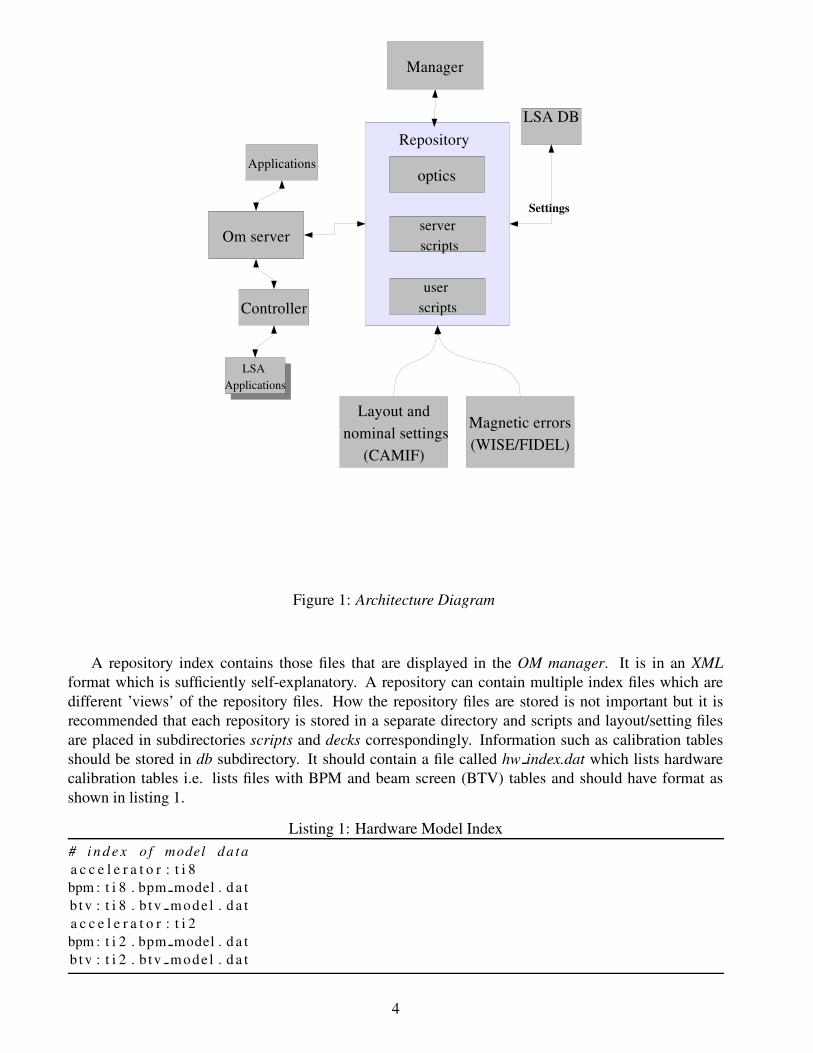
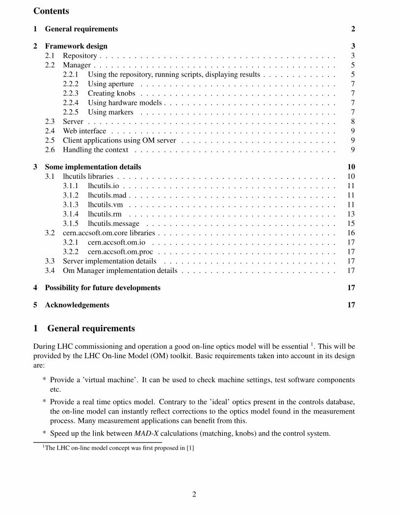
Figure 1: Architecture Diagram

A repository index contains those files that are displayed in the OM manager. It is in an XMLformat which is sufficiently self-explanatory. A repository can contain multiple index files which aredifferent ’views’ of the repository files. How the repository files are stored is not important but it isrecommended that each repository is stored in a separate directory and scripts and layout/setting filesare placed in subdirectories scripts and decks correspondingly. Information such as calibration tablesshould be stored in db subdirectory. It should contain a file called hw index.dat which lists hardwarecalibration tables i.e. lists files with BPM and beam screen (BTV) tables and should have format asshown in listing 1.

Listing 1: Hardware Model Index# i n d e x o f model da taa c c e l e r a t o r : t i 8bpm : t i 8 . bpm model . d a tb t v : t i 8 . b tv mode l . d a ta c c e l e r a t o r : t i 2bpm : t i 2 . bpm model . d a tb t v : t i 2 . b tv mode l . d a t

4

Figure 2: Software Packages

BTV and BPM calibration tables are in obvious column format, for example

Listing 2: Example of a BPM calibration table# s p s bpm model da ta i n c l u d i n g gain , c o u p l i n g , o f f s e t and random e r r o r# r measured = a r t r u e + b + e# f o r m a t : name b 1 b 2 a 11 a 12 a 21 a 22 a b s e r r o r x a b s e r r o r y s t a t u sbpck . 6 1 0 0 1 5 0 0 1 0 0 1 0 . 0 0 0 1 0 . 0 0 0 1 Onbpck . 6 1 0 2 1 1 0 0 1 0 0 1 0 . 0 0 0 1 0 . 0 0 0 1 Onbpck . 6 1 0 3 1 2 0 0 1 0 0 1 0 . 0 0 0 1 0 . 0 0 0 1 Onbpck . 6 1 0 3 4 0 0 0 1 0 0 1 0 . 0 0 0 1 0 . 0 0 0 1 Onbpck . 6 1 0 5 3 9 0 0 1 0 0 1 0 . 0 0 0 1 0 . 0 0 0 1 On

A GUI to handle this information is provided with the OM Manager. For example see repository/afs/cern.ch/eng/sl/online/om/repository/ti and repository index file repo.xml.

2.2 Manager

2.2.1 Using the repository, running scripts, displaying results

The OM manager is a graphical development environment coupled to the control system (see Fig. 3).It contains a repository browser, a text editor, table and graphical output windows. First a repositoryindex should be loaded ( File → Open and select an appropriate xml index file). This will fill therepository browser with script and layout files. Selecting a file in the browser displays it in the editorwindow. File is saved by pressing Ctrl+S. If a script is selected it can be run by pressing Ctrl+X orclicking right mouse button and selecting Save from the menu. A short comment can be added to the

5

script by selecting Properties in the menu. From the same menu scripts can be deleted. A new scriptcan be added to the repository with File → New Script or File → New Python Script dependingon if the script is a mad-x script or a python script.

A script normally produces output tables in the TFS format. The list of produced tables can be seenin the data browser. (see Fig. 4 ). Select a TFS file, then select the Plot tab in the output window. Theaxes to plot are in the drop-down lists. If the hold checkbox is selected the new plot will be drawn ontop of the old one every time a new axis or file is selected. In the same way data in SDDS format canbe displayed. Data file types are determined by the file extension (.sdds, .tfs). Files with extension .yaspare orbit files in TFS format which are placed in a separate subtree for convenience.

Figure 3: OM manager - general view

Figure 4: OM manager - data browser

6

2.2.2 Using aperture

The OM Manager can load aperture tables Tools → Set Aperture. The aperture table should be inthe following TFS format∗ S NAME X Y APER 1 APER 2 APER 3 APER 4

S is the aperture point position, NAME is the element name or label (it will be shown in the apertureplot when the point is clicked upon), APER 1,2,3,4 are the aperture rectellipse coordinates in standardMAD-X convention and X.Y the aperture offsets with respect to the nominal orbit.

2.2.3 Creating knobs

Settings computed by the on-line model such as orbit bumps can be stored in a form of a knob which is alist of magnet settings which can be imported into the control system and applied in fractions. There areseveral ways of creating a knob file, e.g. any python script which will produce a list of magnet settingslikeRBIV . 6 1 0 0 1 3 /K 8 . 8 3 7 6 6 8 1 1 6 e−05RBIV . 6 1 0 3 0 4 /K 8 . 8 8 3 5 8 7 2 3 3 e−05

and write it out to a file with a .knob extension will do. Since the MAD-X strength names and thepower converter names (LSA-NAMES) are different a mapping is provides by ElementTable class inelements.py file in each repositorye t = Elemen tTab le ( )mad name = e t . l sa2mad ( l s a n a m e )l s e n a m e = e t . mad2lsa ( mad name )

Methods to create MAD-X jobs for producing knobs as well as extract the settings from the MAD-X output are provided in knob.py. For example, running a MAD-X job, extracting all strings like‘PAR=VAL’ from the output and converting the parameters to device names is done with one lineknob . run mad ( ’ f i l e . madx ’ , ’bump . knob ’ )

Exporting knobs in the control system follows by selecting the knob from the Knobs tree in the databrowser and clicking Export in the pop-up menu (see Fig. 5).

2.2.4 Using hardware models

Hardware models are hardware calibration tables which could be used, for example, in the orbit loadingfrom the VirtualMachine methods (see also Sec. 3.1.3). A GUI to handle these tables is provided (seeFig. 6).

2.2.5 Using markers

A list of markers can be stored in the file markers.dat in the db subdirectory of a repository. This allowsto store additional information (see. e.g. Fig. 7). Markers can be made visible or invisible by changingthe Active attribute. The list of markers can be edited with Tools → Marker Editor (see Fig. 6). Theformat of the marker file is

Listing 3: Marker List# markers : name a c c e l e r a t o r pos t y p e a c t i v el h c i n j t i 2 l h c 3 1 8 8 . 3 8 4 marker f a l s ei p 2 t i 2 l h c 3 3 3 1 . 4 5 5 1 6 3 marker f a l s eq5 t i 2 l h c 3 1 6 5 . 8 2 marker f a l s e

7

Figure 5: OM manager - creating knobs

Figure 6: OM manager - marker editor and hardware model editor

2.3 Server

The OM Server provides calculations to application software. The control system provides an appliedprogramming interface (API) to send settings or retrieve data from a virtual accelerator rather than areal one. This can be used to develop software when the real data is not yet available and to providea virtual machine for safety. API to connect to the server and send requests is provided. A requestcan contain the accelerator context (cycle, time, etc.), request type (’check-settings’,’get-optics’ etc)

8

Figure 7: OM manager - markers

and a set of parameters (e.g. magnet strength trims). Based on the request type the server launchesa certain computation while the client application waits for the response. The response contains a setof parameters (if some matching was requested), the resulting optics, error or warning messages andseveral other things. Within LSA a higher level interface which hides the details of the server protocolis provided.

2.4 Web interface

CGI-based web interface was developed for some of the applications

http://iagapov.web.cern.ch/iagapov/cgi-bin/om_web.py

It is mostly intended for applications like downloading machine model for use in third-party applica-tions. At this time the development of the CGI interface is discontinued.

2.5 Client applications using OM server

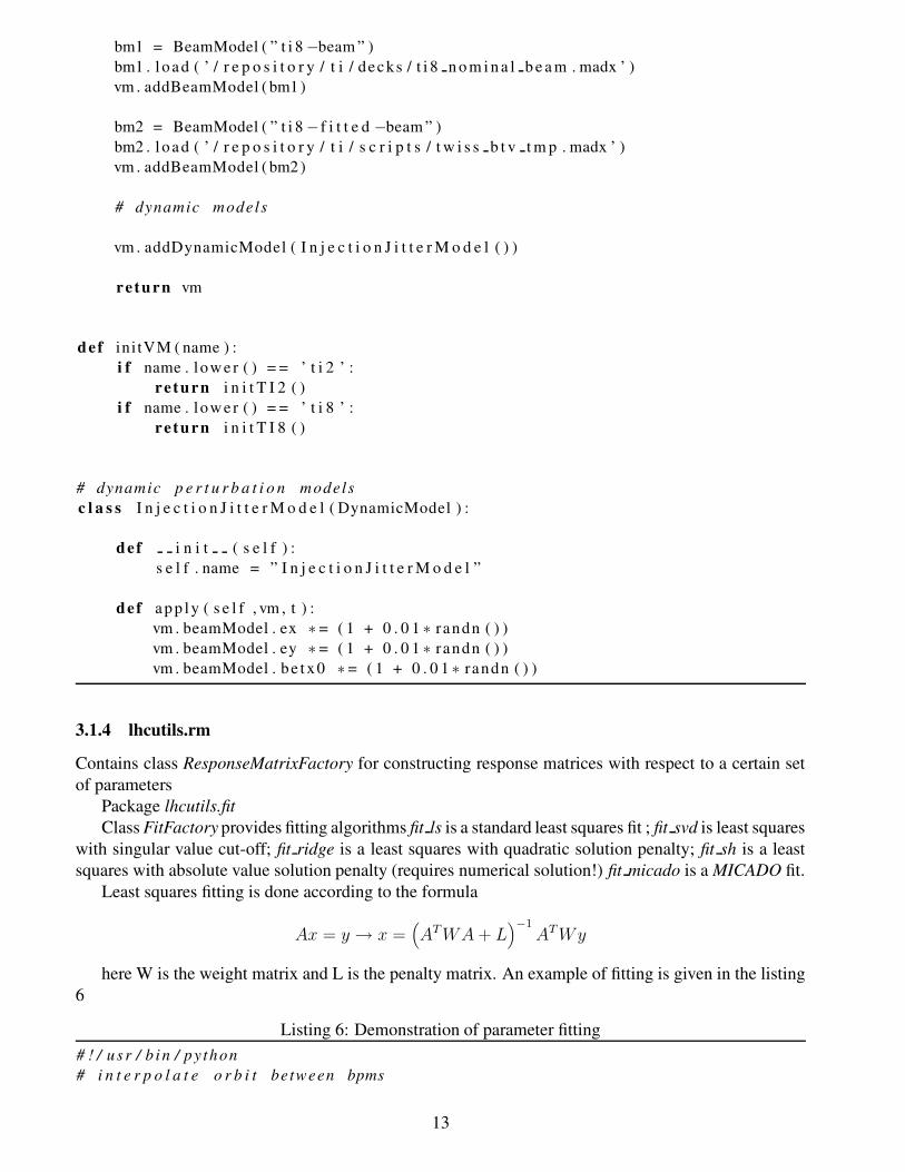
Screenshots of two application using the OM server are shown in Fig. 8 and Fig. 9. The first one(LSA-MADX) sends a trim to the on-line model server using an interface very similar to the applicationto trim machine parameters. It displays the returned optics functions in a pop-up window. The second(LSA-KNOBS) creates certain types of knobs using the server.

2.6 Handling the context

At present the on-line model in the manager mode does not have a built-in context (i.e. optics ) selection.A corresponding optics file selection should be typed in manually in the script corresponding to themachine state under study. In the server mode there is a mapping from the standard LHC context (beamprocess, time, etc.) to the optics file (see implementation details section). A GUI for writing out settingsfile corresponding to a particular machine context was developed by C. Chesneau.

9

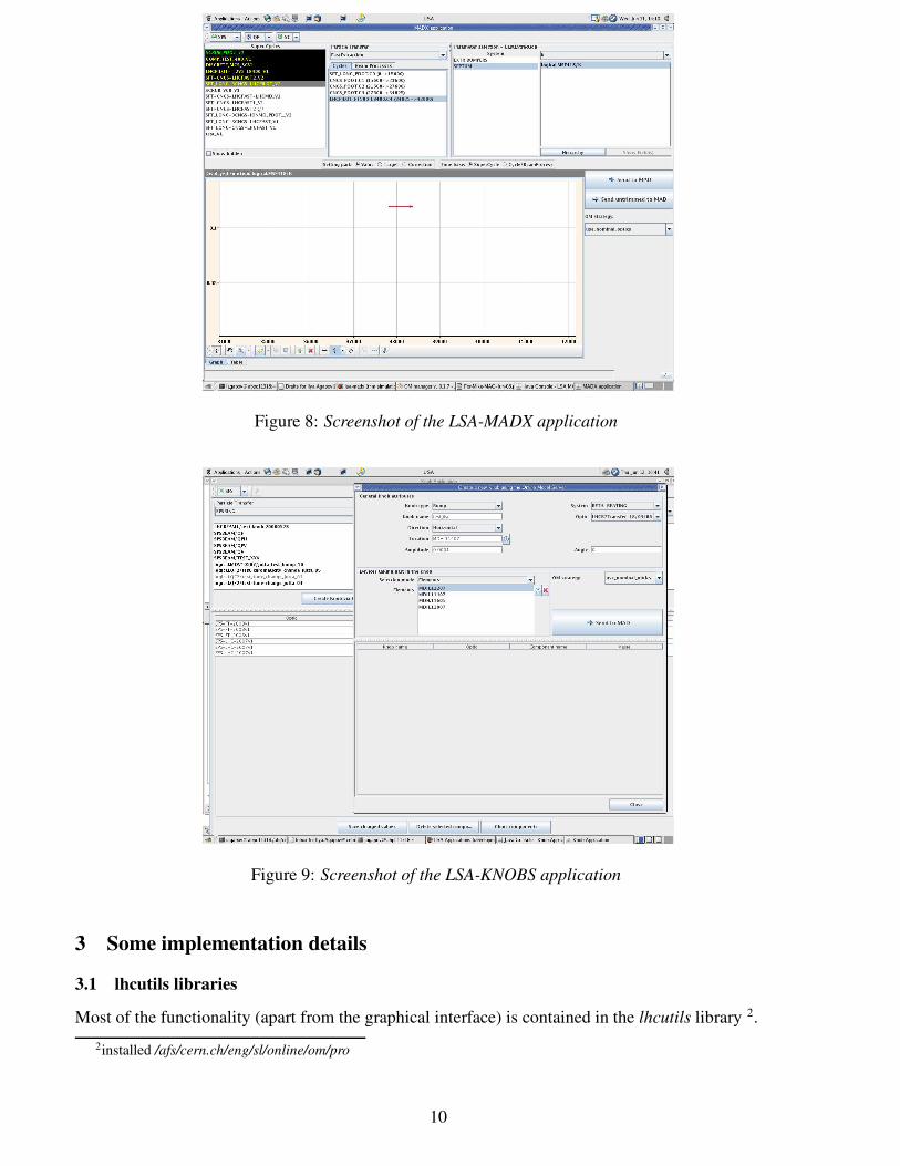
Figure 8: Screenshot of the LSA-MADX application

Figure 9: Screenshot of the LSA-KNOBS application

3 Some implementation details3.1 lhcutils libraries

Most of the functionality (apart from the graphical interface) is contained in the lhcutils library 2.2installed /afs/cern.ch/eng/sl/online/om/pro

10

3.1.1 lhcutils.io

Contains classes for IO and data processing for MAD-X and control system. This includes TFSReader,TFSWriter (MAD-X input/output format), SDDSReader, SDDSWriter (standard for control system mea-surement output).

3.1.2 lhcutils.mad

Provides high-level interface for sequence manipulations and running MAD-X scrips.lhcutils.mad.madx extract.extract warnings and lhcutils.mad.madx extract.extract values for getting

the values (value MAD-X command) and warnings from the MAD-X output.lhcutils.mad.madx test.Tester is a also class for running scripts and getting diagnostics.MADScript is a class for automatic script generation.lhcutils.mad.madx input.MADSequence is a MAD-X parser which can build internal representation

of the MAD-X input, manipulate it and write it out.

Listing 4: Example of processing the input using lhcutils.mad.madx input.MADSequence parser# s e t a p e r t u r e t o l e r a n c e s t o p a r e n t e l e m e n t v a l u e sfrom l h c u t i l s . mad . madx inpu t import ∗

m = MADSequence ( )m. r e a d s e q u e n c e s ( ’V6 . 5 . s eq ’ )m. r e a d s e q u e n c e s ( ’ l h c d e f a u l t m a g t o l e r a n c e s . madx ’ )m. r e a d s e q u e n c e s ( ’ a p e r t o l . b1 . madx ’ )m. r e a d p r o f i l e s ( ’ l h c m e c h a x i s−b1 . madx ’ )m. w r i t e e l e m e n t d e f s ( ’ a p e r t o l ’ , ’ l h c b 1 ’ , ’ l h c b 1 o l d t o l s . madx ’ )

f o r i in xrange ( 0 , l e n (m. e l e m e n t s ) ) :i f m. e l e m e n t s [ i ] . p i d > 0 :p e l = m. e l e m e n t s [m. e l e m e n t s [ i ] . p i d ]p a r e n t t o l s = p e l . g e t p a r a m e t e r ( ’ a p e r t o l ’ )t h i s t o l s = m. e l e m e n t s [ i ] . g e t p a r a m e t e r ( ’ a p e r t o l ’ )i f p a r e n t t o l s = = 0 :

m. e l e m e n t s [ i ] . s e t p a r a m e t e r ( ’ a p e r t o l ’ , n e w t o l s )

3.1.3 lhcutils.vm

Virtual accelerator classes provide a high-level interface to optics computations. A virtual accelerator isrepresented by an object of type VirtualMachine which includes sets of following objects:

BPMModel - BPM models including offsets, calibrations etc. Methods to store and read the BPMcalibration tables. Methods to translate between actual orbit and BPM readings.

BTVModel - beam size measurement models including offsets, calibrations etc. Methods to store andread the calibration tables. Methods to translate between actual beam size measurements and hardwarereadings.

BeamModel - beam parameters including energy, emittance, initial Twiss parameters for a transferline, methods to save and load this parameters from a file.

OpticsModel - includes pointers to sequence and setting files.Orbit - closed orbit data. Contains methods for reading in the orbit data and interpolating it between

BPM locations.DynamicsModel - placeholders for beam dynamics models such as beam jitter.A typical life cycle of the VirtualMachine object in the ‘inference mode’ is to be initialized from a

set of MAD-X decks, be passed to model fitting routines (so that they can create response matrices and

11

so on), be passed to model inference routines (which merge different fits), apply model correction anddump a set of MAD-X decks. In the ‘simulation mode’ the VirtualMachine object is initialized, imper-fections applied, dynamic models attached, observation points and output drivers set and the simulationfired. An example of setting up of the virtual accelerator class is given in listing 5

Listing 5: init.py Demonstration of a virtual accelerator set-up# s e t up t h e v u r t u a l machine − TI2 and TI8

from l h c u t i l s . vm import ∗from numpy . random import ∗

# v i r t u a l machine i n i t i a l i z a t i o ndef i n i t T I 2 ( ) :

vm = V i r t u a l M a c h i n e ( ” t i 2 ” )vm . t y p e = ’ t r a n s f e r ’

# o p t i c s models

om = Opt icsModel ( ” l h c b 1 t r a n s f e r 2 0 0 7 v 1 ” )om . s e q u e n c e f i l e s = [ ’ / r e p o s i t o r y / t i / decks / TI2 . s eq ’ ,

’ / r e p o s i t o r y / t i / decks / TI2 . s t r ’ ]om . m a d x m o d e l f i l e = ’ / r e p o s i t o r y / t i / s c r i p t s / t i 2 m o d e l . madx ’vm . addOpt i c sMode l (om)

# beam models

bm = BeamModel ( ” t i 2 −beam ” )bm . l o a d ( ’ / r e p o s i t o r y / t i / decks / t i 2 n o m i n a l b e a m . madx ’ )vm . addBeamModel (bm)

# dynamic models

vm . addDynamicModel ( I n j e c t i o n J i t t e r M o d e l ( ) )vm . addDynamicModel ( QuadErrorModel ( ) )

re turn vm

def i n i t T I 8 ( ) :vm = V i r t u a l M a c h i n e ( ’ t i 8 ’ )vm . t y p e = ’ t r a n s f e r ’

# o p t i c s models

om = Opt icsModel ( ” l h c b 2 t r a n s f e r 2 0 0 7 v 1 ” )om . s e q u e n c e f i l e s = [ ’ / r e p o s i t o r y / t i / decks / TI8 . s eq ’ ,

’ / r e p o s i t o r y / t i / decks / TI8 . s t r ’ ]om . m a d x m o d e l f i l e = ’ / r e p o s i t o r y / t i / s c r i p t s / t i 8 m o d e l . madx ’vm . addOpt i c sMode l (om)

# beam models

12

bm1 = BeamModel ( ” t i 8 −beam ” )bm1 . l o a d ( ’ / r e p o s i t o r y / t i / decks / t i 8 n o m i n a l b e a m . madx ’ )vm . addBeamModel ( bm1 )

bm2 = BeamModel ( ” t i 8 − f i t t e d −beam ” )bm2 . l o a d ( ’ / r e p o s i t o r y / t i / s c r i p t s / t w i s s b t v t m p . madx ’ )vm . addBeamModel ( bm2 )

# dynamic models

vm . addDynamicModel ( I n j e c t i o n J i t t e r M o d e l ( ) )

re turn vm

def in i tVM ( name ) :i f name . lower ( ) = = ’ t i 2 ’ :

re turn i n i t T I 2 ( )i f name . lower ( ) = = ’ t i 8 ’ :

re turn i n i t T I 8 ( )

# dynamic p e r t u r b a t i o n modelsc l a s s I n j e c t i o n J i t t e r M o d e l ( DynamicModel ) :

def i n i t ( s e l f ) :s e l f . name = ” I n j e c t i o n J i t t e r M o d e l ”

def a p p l y ( s e l f , vm , t ) :vm . beamModel . ex ∗ = ( 1 + 0 . 0 1 ∗ r andn ( ) )vm . beamModel . ey ∗ = ( 1 + 0 . 0 1 ∗ r andn ( ) )vm . beamModel . b e t x 0 ∗ = ( 1 + 0 . 0 1 ∗ r andn ( ) )

3.1.4 lhcutils.rm

Contains class ResponseMatrixFactory for constructing response matrices with respect to a certain setof parameters

Package lhcutils.fitClass FitFactory provides fitting algorithms fit ls is a standard least squares fit ; fit svd is least squares

with singular value cut-off; fit ridge is a least squares with quadratic solution penalty; fit sh is a leastsquares with absolute value solution penalty (requires numerical solution!) fit micado is a MICADO fit.

Least squares fitting is done according to the formula

Ax = y → x =

(

AT WA + L)

−1

AT Wy

here W is the weight matrix and L is the penalty matrix. An example of fitting is given in the listing6

Listing 6: Demonstration of parameter fitting# ! / u s r / b i n / py thon# i n t e r p o l a t e o r b i t be tween bpms

13

from l h c u t i l s . i o import ∗from l h c u t i l s . f i t import ∗from l h c u t i l s . vm import ∗from l h c u t i l s . rm import ∗from i n i t import ∗

from numpy import ∗from numpy . l i n a l g import ∗

import sys , os

def f i t d i s p e r s i o n ( r f , f f , m e s f i l e , r e f f i l e , dxordy , madx ou t f ) :

# g e t t h e measurementr = TFSReader ( m e s f i l e )c o l = r . g e t p a r a m e t e r ( dxordy )names = r . g e t p a r a m e t e r ( ’ name ’ )

r0 = TFSReader ( r e f f i l e )f l t r = { }f l t r [ ’ name ’ ]= r . g e t p a r a m e t e r ( ’ name ’ )

r0 . f i l t e r s = f l t rc o l 0 = r0 . g e t p a r a m e t e r ( dxordy )

n = l e n ( c o l )x = n d a r r a y ( [ n , 1 ] )

p r i n t np r i n t l e n ( c o l 0 )

f o r i in xrange ( 0 , n ) :i f names [ i ] . f i n d ( ’ . B2 ’ ) >0:

x [ i , 0 ] = − e v a l ( c o l [ i ])− e v a l ( c o l 0 [ i ] )e l s e :

x [ i , 0 ] = e v a l ( c o l [ i ])− e v a l ( c o l 0 [ i ] )

r f . debug = Truer f . o b s p a t t e r n s = r . g e t p a r a m e t e r ( ” name ” )r f . o b s e r v s = [ dxordy ]

Ax = r f . c r e a t e o r m ( ’ k i c k ’ ) [ 0 ]

# w e i g h t sf f .W = z e r o s ( [ shape ( Ax ) [ 0 ] , shape ( Ax ) [ 0 ] ] )f o r i in [ 0 , 1 , 2 , 3 , 4 , 5 , 6 , 7 , 8 , 9 , 1 0 ] :

f f .W[ i , i ]=1

t h x = f f . f i t r i d g e ( Ax , x )madx commands = [ ]

14

p a r s = r f . v a r i e d p a r a m e t e r s

d e l t a = ModelDel ta ( )

f o r i in xrange ( 0 , l e n ( p a r s ) ) :madx commands . append ( p a r s [ i ] + ’= ’ + s t r ( t h x [ i ] ) + ’+ ’ + p a r s [ i ] + ’ ; ’ )p r i n t p a r s [ i ] + ’= ’ + s t r ( t h x [ i ] ) + ’+ ’ + p a r s [ i ] + ’ ; ’d e l t a . d e l t a s [ p a r s [ i ] ] = t h x [ i ]

m a d x f i l e = ’ tmp ’+ dxordy + ’ d i s p e r s i o n f i t . madx ’

f = open ( m a d x f i l e , ’w’ )

f . w r i t e ( ’ c a l l , f i l e =\” ’+ r f . o p t i c s M o d e l . m a d x m o d e l f i l e + ’ \ ” ;\ n ’ )

f o r c in madx commands :f . w r i t e ( c+ ’\n ’ )

f . w r i t e ( ’ s e l e c t , f l a g = t w i s s , c l e a r ; s e l e c t , f l a g = t w i s s , column=name , s , dx , dy ;\ n ’ )f . w r i t e ( ’ t w i s s , f i l e = ’+ madx ou t f + ’ , b e t x = betx0 , a l f x = a l f x 0 , b e t y = bety0 , a l f y = a l f y 0 , \dx=dx0 , dpx=dpx0 , dy=dy0 , dpy=dpy0 ; s t o p ; \ n ’ )f . c l o s e ( )

os . sys t em ( ’ / a f s / c e r n . ch / eng / s l / o n l i n e / om / madx / l i n u x / madx < ’ + m a d x f i l e )

re turn d e l t a

def t i 8 l h c ( ) :vm = ini tVM ( )r f = R e s p o n s e M a t r i x F a c t o r y (vm . o p t i c s M o d e l s [ ” t i 8 l h c ” ] )f f = F i t F a c t o r y ( )r f . beam = vm . beamModels [ ” t i 8 −beam ” ]r f . v a r p a t t e r n s = [ ’ kmqif8700m ’ , ’ kmqid8710m ’ , ’ kmqif8740 ’ , ’ kmqif8760 ’ ]r f . v a r i n i t = [ ’ dx0 ’ , ’ dpx0 ’ ]f i l e = ’ / tmp / D meas 2 h . t f s ’f f . L = d i a g ( [ 1 0 0 . , 1 0 0 0 0 . , 1 0 0 0 0 . ] ) # w e i g t h sf i t d i s p e r s i o n ( r f , f f , f i l e , ’ / tmp / t w i s s . nomina l . t f s ’ , ’ dx ’ , ’ / tmp / dx . f i t t e d . t f s ’ )

i f n a m e = = ” m a i n ” :t i 8 l h c ( )

3.1.5 lhcutils.message

Contains python API to the on-line model server. An example of using this class is given in the listingbelow.

class Message

Listing 7: Demonstration of server message habdling# ! / u s r / b i n / py thon#

15

# e v a l u a t e s e t t i n g s#

from l h c u t i l s . message import ∗from e l e m e n t s import ∗import t r i mimport sys , os , t ime

o p t i c s p a t h = ’ / a f s / c e r n . ch / eng / s l / o n l i n e / om / r e p o s i t o r y / l h c / decks / ’

p r i n t ’ # ’ + t ime . a s c t i m e ( )p r i n t ’ c h e c k i n g s e t t i n g s f o r ’ + s y s . a rgv [ 2 ]

inmsg = Message ( )inmsg . r e a d ( s y s . a rgv [ 2 ] )o u t f = s y s . a rgv [ 1 ] + os . s ep + s t r ( inmsg . g e t i d ( ) ) + ’ . msg ’t w i s s f = s y s . a rgv [ 1 ] + os . s ep + s t r ( inmsg . g e t i d ( ) ) + ’ . t f s ’s c t i m e = e v a l ( inmsg . g e t t i m e ( ) )beamproces s = inmsg . g e t b e a m p r o c e s s ( )o p t i c s = inmsg . g e t o p t i c s ( )g e o m e t r y f i l e = inmsg . g e t g e o m e t r y f i l e n a m e ( )s t r e n g t h f i l e = inmsg . g e t s t r e n g t h f i l e n a m e ( )beam = ’ b ’+ s t r ( e v a l ( inmsg . ge t beam ( ) ) + 1 )

p r i n t ’ bp= ’ + beamproces s + ’ , t ime = ’ + s t r ( s c t i m e ) + ’\, o p t i c s = ’ + o p t i c s + ’ beam= ’+beamp r i n t ’ t w i s s f i l e ’ + t w i s s f

t r i m s = inmsg . g e t s e t t i n g s ( )

e t = E lemen tTab le ( )

f o r i in xrange ( 0 , l e n ( t r i m s ) ) :t r i m s [ i ] [ 0 ] = e t . l sa2mad ( t r i m s [ i ] [ 0 ] )p r i n t t r i m s [ i ] [ 0 ] + ’ : ’ + t r i m s [ i ] [ 1 ] + ’ + ’ + t r i m s [ i ] [ 2 ]

t m p m a d x f i l e = ’ t m p m a d x f i l e . madx ’o p t i c s =” lhc nom mod co l ”t r i m . c r e a t e t r i m m e d t w i s s j o b ( t r i m s , \’ t e m p l a t e . madx ’ , t m p m a d x f i l e , t w i s s f , o p t i c s , beam )summary= t r i m . run mad ( t m p m a d x f i l e )

msg = Message ( )msg . s t a t u s = ’ ok ’msg . d e s c r i p t i o n = summary [ 0 ] . r e p l a c e ( ’ : ’ , ’∗ ’ )msg . t f s f i l e p a t h = t w i s s fmsg . w r i t e ( o u t f )

The next sections provide detail about the graphical environment implementation details.

3.2 cern.accsoft.om.core libraries

This package contains classes used in the server and manager implementations.

16

3.2.1 cern.accsoft.om.io

Contains abstract IO classes DataReader and DataWriter and implementations for particular formats -TFSReader, TFSWriter, SDDSReader, SDDSWriter,KnobReader, KnobWriter. Contains log manipula-tion classes OmServerLogManager, LogEntry.

3.2.2 cern.accsoft.om.proc

Various data containers. ApertureSlice, ApertureModel - aperture model implementation. Knob - knobimplementation. ParameterSetting, ParameterSettings - parameter lists used in the knob implementa-tion. SimulationManager - executing MAD-X and python scripts in a separate thread. OpticsModelcontains data and methods to store, read and write optics models in the MAD-X format. It is used togenerate input files from settings in the control system.

3.3 Server implementation details

Package cern.accsoft.om.server contains implementation of the server. Main class is OMServer andmost of the logic is implemented in the task management system (task queue) in the class TaskManager.The server task queue can schedule a number of tasks (which should be implementations of Task abstractclass ) to be executed with certain frequencies. RequestListenerTask defines one such task which listensto connections to the server (i.e. appearances of a message in a predefined directory) and launches anappropriate simulation tasks. Apart from preparing the input the simulation functionality is delegatedto appropriate python code. LSAMessage defines exchange message protocol. LSAMessagePlain andLSAMessageXML are implementations of this protocol with files written in either a simple semicolon-separated or XML formats.

3.4 Om Manager implementation details

Package cern.accsoft.om.manager contains components which implement the Om Manager.

4 Possibility for future developmentsWhile we can consider the general framework of the LHC on-line model finished, the following itemscan be considered as the plan for next years

- Improving on the model inference and fitting functionality.- Tighter integration into the control system (automatic orbit updates, setting updates).- Including non-madx machine models (PTC).

5 AcknowledgementsI wish to thank G. Arduini, E. Benedetto, C. Chesneau, B. Goddard, M. Giovannozzi, W. Herr, V. Kain,G. Kruk, M. Lamont, M. Meddahi, J. Netzel, F. Roncarolo, F. Schmidt, R. Tomas, G. Vanbavinckhoveand J. Wenninger for various forms of support.

References[1] I. Agapov et al. , ’LHC Online model’, proc. PAC 07[2] LHC online model wiki pages,

http://wikis.cern.ch/display/OnlineModel/MADX+On+Line+Model+WikiHome

17

[3] The LHC Injection Tests , CERN-LHC-Performance-Note-001[4] Y. Roblin et al., JLAB-ACE-01-10, 2001.[5] T. Satogata et al., Proc. PAC 1999.[6] M. Woodley et al., ATF2 flight simulator

18