THE LEVERAGE CYCLE

By

John Geanakoplos

July 2009 Revised January 2010

COWLES FOUNDATION DISCUSSION PAPER NO. 1715R

COWLES FOUNDATION FOR RESEARCH IN ECONOMICS YALE UNIVERSITY

Box 208281 New Haven, Connecticut 06520-8281

http://cowles.econ.yale.edu/

The Leverage Cycle

John Geanakoplos�

Revised, January 5, 2010

Abstract

Equilibrium determines leverage, not just interest rates. Variations in lever-age cause �uctuations in asset prices. This leverage cycle can be damaging tothe economy, and should be regulated.Key Words: Leverage, Collateral, Cycle, Crisis, RegulationJEL: E3, E32, G01, G12

1 Introduction to the Leverage Cycle

At least since the time of Irving Fisher, economists, as well as the general public, haveregarded the interest rate as the most important variable in the economy. But in timesof crisis, collateral rates (equivalently margins or leverage) are far more important.Despite the cries of newspapers to lower the interest rates, the Fed would sometimesdo much better to attend to the economy-wide leverage and leave the interest ratealone.When a homeowner (or hedge fund or a big investment bank) takes out a loan

using say a house as collateral, he must negotiate not just the interest rate, but howmuch he can borrow. If the house costs $100 and he borrows $80 and pays $20 incash, we say that the margin or haircut is 20%, the loan to value is $80/$100 =80%, and the collateral rate is $100/$80 = 125%. The leverage is the reciprocal ofthe margin, namely the ratio of the asset value to the cash needed to purchase it, or$100/$20 = 5. These ratios are all synonomous.In standard economic theory, the equilibrium of supply and demand determines

the interest rate on loans. It would seem impossible that one equation could determinetwo variables, the interest rate and the margin. But in my theory, supply and demanddo determine both the equilibrium leverage (or margin) and the interest rate.It is apparent from everyday life that the laws of supply and demand can determine

both the interest rate and leverage of a loan: the more impatient borrowers are,the higher the interest rate; the more nervous the lenders become, or the higher

�James Tobin Professor of Economics, Yale University, and External Professor, Santa Fe Institute.

1

volatility becomes, the higher the collateral they demand. But standard economictheory fails to properly capture these e¤ects, struggling to see how a single supply-equals-demand equation for a loan could determine two variables: the interest rateand the leverage. The theory typically ignores the possibility of default (and thus theneed for collateral), or else �xes the leverage as a constant, allowing the equation topredict the interest rate.Yet variation in leverage has a huge impact on the price of assets, contributing to

economic bubbles and busts. This is because for many assets there is a class of buyerfor whom the asset is more valuable than it is for the rest of the public (standard eco-nomic theory, in contrast, assumes that asset prices re�ect some fundamental value).These buyers are willing to pay more, perhaps because they are more optimistic, orthey are more risk tolerant, or they simply like the assets more. If they can get theirhands on more money through more highly leveraged borrowing (that is, getting aloan with less collateral), they will spend it on the assets and drive those prices up.If they lose wealth, or lose the ability to borrow, they will buy less, so the asset willfall into more pessimistic hands and be valued less.In the absence of intervention, leverage becomes too high in boom times, and too

low in bad times. As a result, in boom times asset prices are too high, and in crisistimes they are too low. This is the leverage cycle.Leverage dramatically increased in the United States and globally from 1999 to

2006. A bank that in 2006 wanted to buy a AAA-rated mortgage security couldborrow 98.4% of the purchase price, using the security as collateral, and pay only1.6% in cash. The leverage was thus 100 to 1.6, or about 60 to 1. The average leveragein 2006 across all of the US$2.5 trillion of so-called �toxic�mortgage securities wasabout 16 to 1, meaning that the buyers paid down only $150 billion and borrowedthe other $2.35 trillion. Home buyers could get a mortgage leveraged 35 to 1, withless than a 3% down payment. Security and house prices soared.Today leverage has been drastically curtailed by nervous lenders wanting more

collateral for every dollar loaned. Those toxic mortgage securities are now (in Q22009) leveraged on average only about 1.2 to 1. A homeowner who bought his housein 2006 by taking out a subprime mortgage with only 3% down cannot take outa similar loan today without putting down 30% (unless he quali�es for one of thegovernment rescue programs). The odds are great that he wouldn�t have the cashto do it, and reducing the interest rate by 1 or 2% won�t change his ability to act.De-leveraging is the main reason the prices of both securities and homes are stillfalling.The leverage cycle is a recurring phenomenon. The �nancial derivatives crisis

in 1994 that bankrupted Orange County in California was the tail end of a lever-age cycle. So was the emerging markets mortgage crisis of 1998, which brought theConnecticut-based hedge fund Long-Term Capital Management to its knees, prompt-ing an emergency rescue by other �nancial institutions. The crash of 1987 also seemsto be at the tail end of a leverage cycle. In the following diagram the average margin

2

23

­

5

10

15

20

25

30

35

40

45

Jun­

98

Dec

­98

Jun­

99

Dec

­99

Jun­

00

Dec

­00

Jun­

01

Dec

­01

Jun­

02

Dec

­02

Jun­

03

Dec

­03

Jun­

04

Dec

­04

Jun­

05

Dec

­05

Jun­

06

Dec

­06

Jun­

07

Dec

­07

Jun­

08

Rep

urch

ase 

Hai

rcut

 (%)

Average Repurchase Haircut on a Portfolio of CMOs Estimated Average Haircut

All CMO margins at Ellington

o¤ered by dealers for all securities purchased at the hedge fund Ellington Capitalis plotted against time. (The leverage Ellington actually used was generally far lessthan what was o¤ered). One sees that the margin was around 20% and then spikeddramatically in 1998 to 40% for a few months, then fell back to 20% again. In late2005 through 2007 the margins fell to around 10%, but then in the crisis of late 2007they jumped to over 40% again, and kept rising for over a year. In Q2 2009 theyreached 70% or more.The policy implication of my theory of equilibrium leverage is that the fed should

manage system wide leverage, curtailing leverage in normal or ebullient times, andpropping up leverage in anxious times. The theory challenges the "fundamentalvalue" theory of asset pricing and the e¢ cient markets hypothesis.If agents extrapolate blindly, assuming from past rising prices that they can safely

set very small margin requirements, or that falling prices means that it is necessaryto demand absurd collateral levels, then the cycle will get much worse. But a crucialpart of my leverage cycle story is that every agent is acting perfectly rationally fromhis own individual point of view. People are not deceived into following illusorytrends. They do not ignore danger signs. They do not panic. They look forward,not backward. But under certain circumstances the cycle spirals into a crash anyway.The lesson is that even if people remember this leverage cycle, there will be moreleverage cycles in the future, unless the Fed acts to stop them.The crash always involves the same three elements. First is scary bad news that

3

increases uncertainty, and so volatility of asset returns. This leads to tighter marginsas lenders get more nervous. This in turn leads to falling prices and huge losses bythe most optimistic, leveraged buyers. All three elements feed back on each other; theredistribution of wealth from optimists to pessimists further erodes prices, causingmore losses for optimists, and steeper price declines, which rational lenders anticipate,leading then to demand more collateral, and so on.The best way to stop a crash is to act long before it occurs, by restricting leverage

in ebullient times.To reverse the crash once it has happened requires reversing the three causes.

In today�s environment, reducing uncertainty means �rst of all stopping foreclosuresand the free fall of housing prices. The only reliable way to do that is to write downprincipal. Second, leverage must be restored to sane, intermediate levels. The Fedmust step around the banks and lend directly to investors, at more generous collaterallevels than the private markets are willling to provide. And third, the Treasurymust inject optimistic capital to make up for the lost buying power of the bankruptleveraged optimists. This might also entail bailing out various crucial players.My theory is of course not completely original. Over 400 years ago in the Merchant

of Venice, Shakespeare explained that to take out a loan one had to negotiate both theinterest rate and the collateral level. It is clear which of the two Shakespeare thoughtwas the more important. Who can remember the interest rate Shylock charged An-tonio? (It was zero percent.) But everybody remembers the pound of �esh thatShylock and Antonio agreed on as collateral. The upshot of the play, moreover, isthat the regulatory authority (the court) decides that the collateral Shylock and An-tonio freely agreed upon was socially suboptimal, and the court decrees a di¤erentcollateral: a pound of �esh but not a drop of blood. The Fed too should sometimesdecree di¤erent collateral rates.In more recent times there has been pioneering work on collateral by Shleifer and

Vishny SV (1992), Bernanke, Gertler, Gilchrist BGG (1996, 1999), and Holmstromand Tirole (1997). This work emphasized the asymmetric information between bor-rower and lender, leading to a principal agent problem. For example, in SV (1992),the debt structure of short vs long loans must be arranged to discourage the �rm man-agement from undertaking negative present value investments with personal perks inthe good state. But in the bad state this forces the �rm to liquidate, just when othersimilar �rms are liquidating, causing a price crash. In HT (1997) the managers ofa �rm are not able to borrow all the inputs necessary to build a project, becauselenders would like to see them bear risk, by putting their own money down, to guar-antee that they exert maximal e¤ort. The BGG (1999) model, adapted from theirearlier work, is cast in an environment with costly state veri�cation. It is closelyrelated to the second example I give below, with utility from housing and foreclo-sure costs, taken from Geanakoplos (1997). But an important di¤erence is that Ido not invoke any asymmetric information. I believe that it is important to notethat endogenous leverage need not be based on asymmetric information. Of course

4

the asymmetric information revolution in economics was a tremendous advance, andasymmetric information plays a critical role in many lender-borrower relationships;sometimes, however, the profession becomes obsessed with it. In the crisis of 2007-2009, it does not appear to me that asymmetric information played a critical role insetting margins. Certainly the buyers of mortgage securities did not control their pay-o¤s. In my model the only thing backing the loan is the physical collateral. Becausethe loans are no-recourse, there is no need to learn anything about the borrower. Allthat matters is the collateral. Repo loans, and mortgages in many states, are literallyno-recourse. In the rest of the states lenders rarely come after borrowers for moremoney beyond taking the house. And for subprime borrowers, the hit to the creditrating is becoming less and less tangible. In looking for determinants of (changes in)leverage, one should start with the distribution of collateral payo¤s, and not the levelof asymmetric information.Another important paper on collateral is Kiyotaki and Moore (1997). Like BGG

(1996), this paper emphasized the feedback from the fall in collateral prices to a fallin borrowing capacity, assuming a constant loan to value ratio. By contrast, mywork de�ning collateral equilibrium focused on what determines the ratios (LTV,margin, or leverage) and why they change. In practice, I believe the change inratios has been far bigger and more important for borrowing than the change inprice levels. The possibility of changing ratios is latent in the BGG models, but notemphasized by them. In my 1997 paper I showed how one supply-equals-demandequation can determine leverage as well as interest even when the future is uncertain.In my 2003 paper on the anatomy of crashes and margins (it was an invited addressat the 2000 World Econometric Society meetings), I argued that in normal timesleverage and asset prices get too high, and in bad times, when the future is worseand more uncertain, leverage and asset prices get too low. In the certainty modelof Kiyotaki and Moore, to the extent leverage changes at all, it goes in the oppositedirection, getting looser after bad news. In Fostel-Geanakoplos 2008b, on leveragecycles and the anxious economy, we noted that margins do not move in lock stepacross asset classes, and that a leverage cycle in one asset class might spread to otherunrelated asset classes. In Geanakoplos-Zame (1997, 2002, 2009) we describe thegeneral properties of collateral equilibrium. In Geanakoplos-Kubler (2005), we showthat managing collateral levels can lead to Pareto improvements.1

The recent crisis has stimulated a new generation of important papers on leverageand the economy. Notable among these are Brunnermeier and Pedersen (2009), an-ticipated partly by Gromb and Vayanos (2002), and Adrian and Shin (2009). Adrianand Shin have developed a remarkable series of empirical studies of leverage.It is very important to note that leverage in my paper is de�ned by a ratio of col-

lateral values to the downpayment that must be made to buy them. Those "securitiesleverage" numbers are hard to get historically. I provided an aggregate of them from

1For Pareto improving interventions in credit markets, see also Gromb-Vayanos (2002) and Loren-zoni (2008).

5

the data base of one hedge fund, but as far as I know securities leverage numbers havenot been systematically kept. One absolutely essential innovation would be for theFed to gather these numbers and periodically report leverage numbers across di¤er-ent asset classes. It is much easier to get "investor leverage" (debt + equity)/equityvalues for �rms. But these investor leverage numbers can be very misleading. Whenthe economy goes badly, and the true securities leverage is sharply declining, many�rms will �nd their equity wiped out, and it will appear as though their leveragehas gone up, instead of down. This reversal may explain why some macroeconomistshave underestimated the role leverage plays in the economy.Perhaps the most important lesson from this work (and the current crisis) is that

the macroeconomy is strongly in�uenced by �nancial variables beyond prices. Thisof course was the theme of much of the work of Minsky (1986), who called attentionto the dangers of leverage, and of James Tobin (who in Tobin-Golub (1998) explicitlyde�ned leverage and stated that it should be determined in equilibrium, alongsideinterest rates), and also of Bernanke, Gertler, and Gilchrist.

1.1 Why was this leverage cycle worse than previous cycles?

There are a number of elements that played into the leverage cycle crisis of 2007-9that had not appeared before, which explain why it has been so bad. I will graduallyincorporate them into the model. The �rst I have already mentioned, namely thatleverage got higher than ever before, and then margins got tighter than ever before.The second is the invention of the credit default swap. The buyer of "CDS insur-

ance" gets a dollar for every dollar of defaulted principal on some bond. But he isnot limited to buying as much insurance as he owns bonds. In fact, he very likely isbuying the CDS nowadays because he thinks the bonds are bad and does not wantto own them at all. CDS are, despite their names, not insurance, but a vehicle foroptimists and pessimists to leverage their views. Conventional leverage allows op-timists to push the price of assets up; CDS allows pessimists to push asset pricesdown. The standardization of CDS for mortgages in late 2005 led to their trades inlarge quantities in 2006 at the very peak of the cycle. This I believe was one of theprecipitators of the downturn.Third, this leverage cycle was really a combination of two leverage cyles, in

mortage securities and in housing. The two reinforce each other. The tighteningmargins in securities led to lower security prices, which made it harder to issue newmortgages, which made it harder for homeowners to re�nance, which made themmorelikely to default, which raised required downpayments on housing, which made hous-ing prices fall, which made securities riskier, which made their margins get tighterand so on.Fourth, when promises exceed collateral values, as when housing is "under water"

or "upside down," there are typically large losses in turning over the collateral, partlybecause of vandalism and so on. In the current crisis more houses are underwater

6

than at any time since the Depression. Today subprime bondholders expect only25% of the loan amount back when they foreclose on a home. A huge number ofhomes are expected to be foreclosed (some say 8 million). In the model we will seethat even if borrowers and lenders foresee that the loan amount is so large then therewill be circumstances in which the collateral is under water, and therefore will causedeadweight losses, they will not be able to prevent themselves from agreeing on suchlevels.Fifth, the leverage cycle potentially has a major impact on productive activities

for two reasons. First, investors, like homeowners and banks, that �nd themselvesunder water, even if they have not defauted, no longer have the same incentives toinvest (or make loans). This is called the debt overhang problem (Myers 1977). Highasset prices means strong incentives for production, and a boon to real construction.The fall in asset prices has a blighting e¤ect on new real activity. This is the essenceof Tobin�s Q. And it is the real reason why the crisis stage of the leverage cycle is soalarming.

1.2 Outline

In Sections II and III, I present the basic model of the leverage cycle drawing on my2003 paper, in which a continuum of investors di¤er in their optimism. In the twoperiod model of Section II, I show that the price of an asset rises when it can beleveraged more. The reason is that then fewer optimists are needed to hold all of theasset shares. Hence the marginal buyer, whose opinion determines the asset price, ismore optimistic. One consequence is that �e¢ cient markets�pricing fails; even thelaw of one price fails. If two assets are identical, except that the blue one can beleveraged and the red one not, then the blue asset will often sell for a higher price.Next I show that when news in any period is binary, namely good or bad, then

the equilibrium of supply and demand will pin down leverage so that the promisemade on collateral is the maximum that does not involve any chance of default. Thisis reminiscent of the Repo market, where there is almost never any default. It followsthat if lenders and investors imagine a worse downside for the collateral value whenthe loan comes due, there will be a smaller equilibrium loan, and hence less leverage.In Section III, I again draw on my 2003 paper to study a three-period, binary

tree version of the model presented in Section II. The asset pays out only in the lastperiod, and in the middle period information arrives about the likelihood of the �nalpayo¤s. An important consequence of the no default leverage principle derived inSection II is that loan maturities in the multi-period model will be very short. Somuch can go wrong with the collateral price over several periods that only very littleleverage can avoid default for sure on a long loan with a �xed promise. Investors whowant to leverage a lot will have to borrow short term. This provides one explanationfor the famous maturity mismatch, in which long lived assets are �nanced with shortterm loans. In the model equilibrium, all investors endogenously take out one-period

7

loans, and leverage is reset each period.When news arrives in the middle period, the agents rationally update their beliefs

about �nal payo¤s. I distinguish between bad news, which lowers expectations, and�scary�bad news, which lowers expectations and increases volatility (uncertainty).This latter kind depresses asset prices at least twice, by reducing expected payo¤s onaccount of the bad news and by collapsing leverage on account of the increased volatil-ity. After normal bad news, the asset price drop is often cushioned by improvementsin leverage.When �scary� bad news hits in the middle period, the asset price falls more

than any agent in the whole economy thinks it should. The reason is that threethings deteriorate. In addition to the e¤ect of bad news on expected payo¤s, leveragecollapses. On top of that, the most optimistic buyers (who leveraged their purchasesin the �rst period) go bankrupt. Hence the marginal buyer in the middle period is adi¤erent and much less optimistic agent than in the �rst period.I conclude Section III by describing �ve aspects of the leverage cycle that might

motivate a regulator to smooth it out. Not all of these are formally in the model,but they could be added with little trouble. First, when leverage is high, the price isdetermined by very few �outlier�buyers who might, given the di¤erences in beliefs, bewrong! Second, when leverage is high, so are asset prices, and when leverage collapsesprices crumble. The upshot is that when there is high leverage economic activity isstimulated, when there is low leverage the economy is stagnant. If the prices are drivenby outlier opinions, absurd projects might be undertaken in the boom times that arecostly to unwind in the down times. Third, even if the projects are sensible, manypeople who cannot insure themselves will be subjected to tremendous risk that can bereduced by smoothing the cycle. Fourth, over the cycle inequality can dramaticallyincrease if the leveraged buyers keep getting lucky, and dramatically compress if theleveraged buyers lose out. Finally, it may be that the leveraged buyers do not fullyinternalize the costs of their own bankruptcy, as when a manager does not take intoaccount that his workers will not be able to �nd comparable jobs, or when a defaultercauses further defaults in a chain reaction.In Section IV, I move to a second model, drawn from my 1997 paper, in which

probabilities are objectively given, and heterogeneity among investors arises not fromdi¤erences in beliefs, but from di¤erences in the utility of owning the collateral, aswith housing. Once again, leverage is endogenously determined, but now defaultappears in equilibrium. It is very important to observe that the source of the het-erogeneity has implications for the amount of equilibrium leverage, default, and loanmaturity. In the mortgage market, where di¤erences in utility for the collateral drivethe market, there has always been default (and long maturity loans), even in the bestof times.As in Sections II and III, bad news causes the asset price to crash much further

than it would without leverage. It also crashes much further than it would withcomplete markets. (With objective probabilities, the lovers of housing would insure

8

themselves completely against the bad news and so housing prices would not drop atall.) In the real world, when a house falls in value below the loan and the homeownerdecides to default, he often does not cooperate in the sale, since there is nothing init for him. As a result, there can be huge losses in seizing the collateral. (In theU.S. it takes 18 months on average to evict the owners, the house is often vandalized,and so on.) I show that even if borrowers and lenders recognize that that there areforeclosure costs, and even if they recognize that the further under water the houseis the more di¢ cult the recovery will be in foreclosure, they will still choose leveragethat causes those losses.I conclude Section IV by giving three more reasons, beyond the �ve from Section

III, why we might worry about excessive leverage. Sixth, the market endogenouslychooses loans that lead to foreclosure costs. Seventh, in a multi-period model someagents may be under water, in the sense that the house is worth less than the presentvalue of the loan, but not yet in bankruptcy. These agents often will not take e¢ cientactions. A homeowner may not repair his house, even though the cost is muchless than the increase in value of the house, because there is a good chance he willhave to go into foreclosure. Eighth, agents do not take into account that by over-leveraging their own houses or mortgage securities they create pecuniary externalities;for example, by getting into trouble themselves, they may be lowering housing pricesafter bad news, thereby pushing other people further underwater, and thus creatingmore deadweight losses in the economy.Finally, in Section V, I combine the two previous approaches, imagining a model

with two-period mortgage loans using houses as collateral, and one-period repo loansusing the mortgages as collateral. The resulting double leverage cycle is an essentialelement of our current crisis. Here, all eight drawbacks to excessive leverage appearat once.

1.3 Leverage and Volatility: Scary Bad News

Crises always start with bad news; there are no pure coordination failures. But notall bad news lead to crises, even when the news is very bad.Bad news in my view must be of a special "scary" kind to cause an adverse move

in the leverage cycle. Scary bad news not only lowers expectations (as by de�nition allbad news does), but it must create more volatility. Often this increased uncertaintyalso involves more disagreement. On average news reduces uncertainty, so I have inmind a special, but by no means unusual, kind of news. One kind of scary bad newsmotivates the examples in Sections II and III. The idea is that at the beginning,everyone thinks the chances of ultimate failure require too many things to go wrongto be of any substantial probability. There is little uncertainty, and therefore littleroom for disagreement. Once enough things go wrong to raise the spectre of realtrouble, the uncertainty goes way up in everyone�s mind, and so does the possibilityof disagreement.

9

An example occurs when output is 1 unless two things go wrong, in which caseoutput becomes .2. If an optimist thinks the chance of each thing going wrong isindependent and equal to .1, then it is easy to see that he thinks the chance of ultimatebreakdown is .01=(.1)(.1). Expected output for him is .992. In his view ex ante, thevariance of �nal output is :99(:01)(1� :2)2 = :0063. After the �rst piece of bad new,his expected output drops to .92. But the variance jumps to :9(:1)(1� :2)2 = :058, atenfold increase.A less optimistic agent who believes the probability of each piece of bad news is

independent and equal to :8 originally thinks the probability of ultimate breakdownis :04 = (:2)(:2). Expected output for him is :968. In his view ex ante, the variance of�nal output is :96(:04)(1� :2)2 = :025. After the �rst piece of bad new, his expectedoutput drops to :84. But the variance jumps to :8(:2)(1 � :2)2 = :102. Note thatthe expectations di¤ered originally by :992� :968 = :024, but after the bad news thedisagreement more than triples to :92� :84 = :08.I call the kind of bad news that increases uncertainty and disagreement scary

news.The news in the last 18 months has indeed been of this kind. When agency

mortgage default losses were less than 1/4%, there was not much uncertainty andnot much disagreement. Even if they tripled, they would still be small enough notto matter. Similarly, when subprime mortgage losses (that is losses incurred afterhomeowners failed to pay, were thrown out of their homes, and the house was sold forless than the loan amount) were 3%, they were so far under the rated bond cushionof 8% that there was not much uncertainty or disagreement about whether the bondswould su¤er losses, especially the higher rated bonds (with cushions of 15% or more).By 2007, however, forecasts on subprime losses ranged from 30% to 80%.

1.4 Anatomy of a Crash

I use my theory of the equilibrium leverage to outline the anatomy of market crashesafter the kind of scary news I just described.i) Assets go down in value on scary bad news.ii) This causes a big drop in the wealth of the natural buyers (optimists) who were

leveraged. Leveraged buyers are forced to sell to meet their margin requirements.iii) This leads to further loss in asset value, and in wealth for the natural buyers.iv) Then just as the crisis seems to be coming under control, margin requirements

are tightened because of increased uncertainty and disagreement.v) This causes huge losses in asset values via forced sales.vi) Many optimists will lose all their wealth and go out of businessvii) There may be spillovers if optimists in one asset hit by bad news are led to

sell other assets for which they are also optimists.viii) Investors who survive have a great opportunity.

10

1.5 Heterogeneity and Natural Buyers

A crucial part of my story is heterogeneity between investors. The natural buyers wantthe asset more than the general public. This could be for many reasons. The naturalbuyers could be less risk averse. Or they could have access to hedging techniques thegeneral public does not that make the assets less dangerous for them. Or they couldget more utility out of holding the assets. Or they could have access to a productiontechnology that uses the assets more e¢ ciently than the general public. Or theycould have special information based on local knowledge. Or they could simply bemore optimistic. I have tried nearly all these possibilities at various times in mymodels. In the real world, the natural buyers are probably made up of a mixture ofthese categories. But for modeling purposes, the simplest is the last, namely thatthe natural buyers are more optimistic by nature. They have di¤erent priors fromthe pessimists. I note simply that this perspective is not really so di¤erent fromdi¤erences in risk aversion. Di¤erences in risk aversion in the end just mean di¤erentrisk adjusted probabilities, which appear very similar to di¤erences in belief whenasset payo¤s are correlated with endowments.A loss for the natural buyers is much more important to prices than a loss for the

public, because it is the natural buyers who will be holding the assets and biddingtheir prices up. Similarly, the loss of access to borrowing by the natural buyers (andthe subsequent moving of assets from natural buyers to the public) creates the crash.Current events have certainly borne out this heterogeneity hypothesis. When

the big banks (who are the classic natural buyers) lost lots of capital through theirblunders in the CDO market, that had a profound e¤ect on new investments. Some ofthat capital was restored by international investments from Singapore and so on, butit was not enough, and it quickly dried up when the initial investments lost money.Macroeconomists have often ignored the natural buyers hypothesis. For example,

some macroeconomists compute the marginal propensity to consume out of wealth,and �nd it very low. The loss of $250 billion dollars of wealth could not possiblymatter much they said, because the stock market has fallen many times by muchmore and economic activity hardly changed. But that ignores who lost the money.The natural buyers hypothesis is not original with me. (See for example Harrison

and Kreps (1979), and Shleifer and Vishny (1997).2) The innovation is in combiningit with equilibrium leverage.I do not presume a cut and dried distinction between natural buyers and the

public. In Section II, I imagine a continuum of agents uniformly arrayed between0 and 1. Agent h on that continuum thinks the probability of good news (Up) is hU = h, and the probability of bad news (Down) is

hD = 1 � h. The higher the h,

the more optimistic the agent.The more optimistic an agent, the more natural a buyer he is. By having a

continuum I avoid a rigid categorization of agents. The agents will choose whether to

2See also Caballero-Krishnamurthy (2001) and Fostel-Geanakoplos (2008a).

11

Natural buyers

Public

Natural Buyers Theory of Price

h=b

h=1

h=0

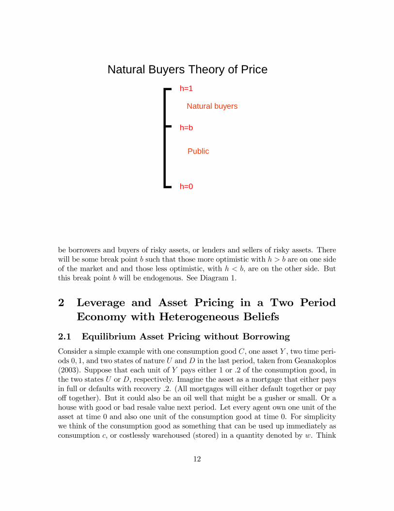
be borrowers and buyers of risky assets, or lenders and sellers of risky assets. Therewill be some break point b such that those more optimistic with h > b are on one sideof the market and and those less optimistic, with h < b; are on the other side. Butthis break point b will be endogenous. See Diagram 1.

2 Leverage and Asset Pricing in a Two PeriodEconomy with Heterogeneous Beliefs

2.1 Equilibrium Asset Pricing without Borrowing

Consider a simple example with one consumption good C, one asset Y , two time peri-ods 0; 1, and two states of nature U and D in the last period, taken from Geanakoplos(2003). Suppose that each unit of Y pays either 1 or .2 of the consumption good, inthe two states U or D, respectively. Imagine the asset as a mortgage that either paysin full or defaults with recovery .2. (All mortgages will either default together or payo¤ together). But it could also be an oil well that might be a gusher or small. Or ahouse with good or bad resale value next period. Let every agent own one unit of theasset at time 0 and also one unit of the consumption good at time 0. For simplicitywe think of the consumption good as something that can be used up immediately asconsumption c, or costlessly warehoused (stored) in a quantity denoted by w. Think

12

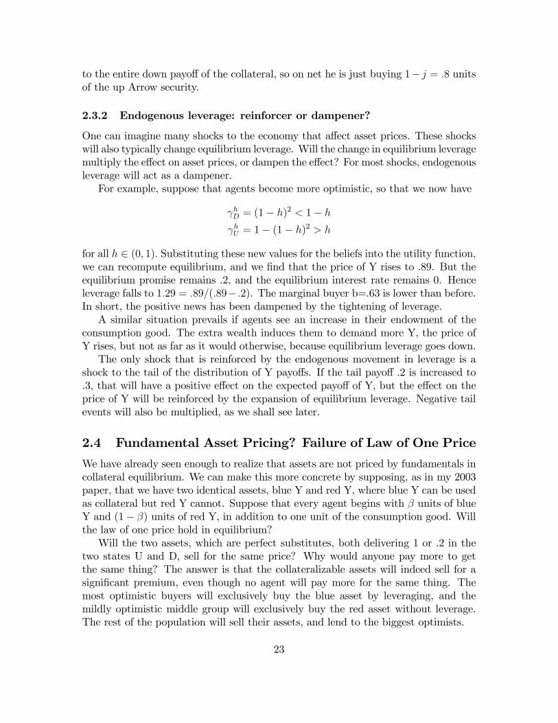
Let each agent h ∈ H ⊂ [0,1]assign probability h to s = Uand probability 1 − h to s = D.Agents with h near 1 areoptimists, agents with h near 0are pessimists.

Endogenous Collateral with HeterogeneousBeliefs: A Simple Example

Suppose that 1 unit of Y gives $1 unit in state U and .2 units in D.

U

D

Y=.2

0

h

1 –h

Figure 2

Y=1

of oil or cigarettes or canned food or simply gold (that can be used as �llings) ormoney. The agents h 2 H only care about the total expected consumption they get,no matter when they get it. They are not impatient. The di¤erence between theagents is only in the probabilities hU ;

hD = 1 � hU each attaches to a good outcome

vs bad.To start with, let us imagine the agents arranged uniformly on a continuum, with

agent h 2 H = [0; 1] assigning probability hU = h to the good outcome.See diagram 2.More formally, denoting the original endowment of goods and securities of agent

h by eh; the amount of consumption of C in state s by cs, and the holding in state sof Y by ys, and the warehousing of the consumption good at time 0 by w0 we have

uh(c0; y0; w0; cU ; cD) = c0 + hUcU +

hDcD = c0 + hcU + (1� h)cD

eh = (ehCo ; ehYo ; e

hCU; ehCD) = (1; 1; 0; 0)

Storing goods and holding assets provide no direct utility, they just increase incomein the future.Suppose the price of the asset per unit at time 0 is p, somewhere between 0 and

1. The agents h who believe that

h1 + (1� h):2 > p

13

will want to buy the asset, since by paying p now they get something with expectedpayo¤ next period greater than p and they are not impatient. Those who think

h1 + (1� h):2 < p

will want to sell their share of the asset. I suppose there is no short selling, but I willallow for borrowing. In the real world it is impossible to short sell many assets otherthan stocks. Even when it is possible, only a few agents know how, and those typicallyare the optimistic agents who are most likely to want to buy. So the assumption ofno short selling is quite realistic. But we shall reconsider this point shortly.If borrowing were not allowed, then the asset would have to be held by a large

part of the population. The price of the asset would be :677 or about :68: Agenth = :60 values the asset at :68 = :60(1)+ :40(:2). So all those h below :60 will sell allthey have, or :60(1) = :60 in aggregate. Every agent above :60 will buy as much ashe can a¤ord. Each of these agents has just enough wealth to buy 1=:68 � 1:5 moreunits, hence :40(1:5) = :60 units in aggregate. Since the market for assets clears attime 0, this is the equilibrium with no borrowing.More formally, taking the price of the consumption good in each period to be 1

and the price of Y to be p, we can write the budget set without borrowing for eachagent as

Bh0 (p) = f(c0; y0; w0; cU ; cD) 2 R5+ : c0 + w0 + p(y0 � 1) = 1cU = w0 + y0

cD = w0 + (:2)y0g:

Given the price p, each agent chooses the consumption plan (ch0 ; yh0 ; w

h0 ; c

h1 ; c

h2) inB

h0 (p)

that maximizes his utility uh de�ned above. In equilibrium all markets must clearZ 1

0

(ch0 + wh0 )dh = 1Z 1

0

yh0dh = 1Z 1

0

chUdh = 1 +

Z 1

0

wh0dhZ 1

0

chDdh = :2 +

Z 1

0

wh0dh

In this equilibrium agents are indi¤erent to storing or consuming right away, so wecan describe equilibrium as if everyone warehoused and postponed consumption bytaking

p = :68

(ch0 ; yh0 ; w

h0 ; c

hU ; c

hD) = (0; 2:5; 0; 2:5; :5) for h � :60

(ch0 ; yh0 ; w

h0 ; c

hU ; c

hD) = (0; 0; 1:68; 1:68; 1:68) for h < :60:

14

2.2 Equilibrium Asset Pricing with Borrowing at ExogenousCollateral Rates

When loan markets are created, a smaller group of less than 40% of the agents willbe able to buy and hold the entire stock of the asset. If borrowing were unlimited, atan interest rate of 0, the single agent at the top would borrow so much that he wouldbuy up all the assets by himself. And then the price of the asset would be 1, since atany price p lower than 1 the agents h just below 1 would snatch the asset away fromh = 1. But this agent would default, and so the interest rate would not be zero, andthe equilibrium allocation needs to be more delicately calculated.

2.2.1 Incomplete Markets

We shall restrict attention to loans that are non-contingent, that is that involvepromises of the same amount ' in both states. It is evident that the equilibriumallocation under this restriction will in general not be Pareto e¢ cient. For example,in the no borrowing equilibrium, everyone would gain from the transfer of " > 0 unitsof consumption in state U from each h < :60 to each agent with h > :60, and thetransfer of 3"=2 units of consumption in state D from each h > :60 to each agent withh < :60. The reason this has not been done in the equilibrium is that there is no assetthat can be traded that moves money from U to D or vice versa. We say that theasset markets are incomplete. We shall assume this incompleteness for a long time,until we consider Credit Default Swaps.

2.2.2 Collateral

We have not yet determined how much people can borrow or lend. In conventionaleconomics they can do as much of either as they like, at the going interest rate. But inreal life lenders worry about default. Suppose we imagine that the only way to enforcedeliveries is through collateral. A borrower can use the asset itself as collateral, sothat if he defaults the collateral can be seized. Of course a lender realizes that if thepromise is ' in both states, then with no-recourse collateral he will only receive

min('; 1) if good news

min('; :2) if bad news

The introduction of collateralized loan markets introduces two more parameters: howmuch can be promised ', and at what interest rate r?Suppose that borrowing were arbitrarily limited to ' � :2y0, that is suppose agents

were allowed to promise at most :2 units of consumption per unit of the collateralY they put up. That is a natural limit, since it is the biggest promise that is sureto be covered by the collateral. It also greatly simpli�es our notation, because thenthere would be no need to worry about default. The previous equilibrium without

15

borrowing could be reinterpreted as a situation of extraordinarily tight leverage, wherewe have the constraint ' � 0y0.Leveraging, that is, using collateral to borrow, gives the most optimistic agents a

chance to spend more. And this will push up the price of the asset. But since theycan borrow strictly less than the value of the collateral, optimistic spending will stillbe limited. Each time an agent buys a house, he has to put some of his own moneydown in addition to the loan amount he can obtain from the collateral just purchased.He will eventually run out of capital.We can describe the budget set formally with our extra variables.

Bh:2(p; r) = f(c0; y0; '0; w0; cU ; cD) 2 R6+ :

c0 + w0 + p(y0 � 1) = 1 +1

1 + r'0

'0 � :2y0cU = w0 + y0 � '0cD = w0 + (:2)y0 � '0g:

We use the subscript :2 on the budget set to remind ourselves that we have arbitrarily�xed the maximum promise that can be made on a unit of collateral. At this pointwe could imagine that was a parameter set by government regulators.Note that in the de�nition of the budget set, '0 > 0 means that the agent is

making promises in order to borrow money to spend more at time 0. Similarly,'0 < 0 means the agent is buying promises which will reduce his expenditures onconsumption and assets in period 0, but enable him to consume more in the futurestates U and D. Equilibrium is de�ned by the price and interest rate (p; r) and agentchoices (ch0 ; y

h0 ; '

h0 ; w

h0 ; c

hU ; c

hD) in B

h:2(p; r) that maximizes his utility u

h de�ned above.In equilibrium all markets must clearZ 1

0

(ch0 + wh0 )dh = 1Z 1

0

yh0dh = 1Z 1

0

'h0dh = 0Z 1

0

chUdh = 1 +

Z 1

0

wh0dhZ 1

0

chDdh = :2 +

Z 1

0

wh0dh

Clearly the no borrowing equilibrium is a special case of the collateral equilibrium,once the limit :2 on promises is replaced by 0.

16

2.2.3 The Marginal Buyer

By simultaneously solving equations (1) and (2) below, one can calculate that theequilibrium price of the asset is now :75. By equation (1), agent h = :69 is justindi¤erent to buying. Those h < :69 will sell all they have, and those h > :69 willbuy all they can with their cash and with the money they can borrow. By equation(2) the top 31% of agents will indeed demand exactly what the bottom 69% areselling.Who would be doing the borrowing and lending? The top 31% is borrowing to

the max, in order to get their hands on what they believe are cheap assetss. Thebottom 69% do not need the money for buying the asset, so they are willing to lendit. And what interest rate would they get? 0% interest, because they are not lendingall they have in cash. (They are lending :2=:69 = :29 < 1 per person). Since they arenot impatient and they have plenty of cash left, they are indi¤erent to lending at 0%.Competition among these lenders will drive the interest rate to 0%.More formally, letting the marginal buyer be denoted by h = b; we can de�ne the

equilibrium equations as

p = bU1 + (1� bU)(:2) = b1 + (1� b)(:2) (1)

p =(1� b)(1) + :2

b(2)

Equation (1) says that the marginal buyer b is indi¤erent to buying the asset.Equation (2) says that the price of Y is equal to the amount of money the agentsabove b spend buying it, divided by the amount of the asset sold. The numerator isthen all the top group�s consumption endowment, (1� b)(1); plus all they can borrowafter they get their hands on all of Y, namely (1)(:2)=(1 + r) = :2: The denominatoris comprised of all the sales of one unit of Y each by the agents below b:We must also take into account buying on margin. An agent who buys the asset

while simultaneously selling as many promises as he can will only have to pay downp � :2: His return will be nothing in the down state, because then he will have toturn over all the collateral to pay back his loan. But in the up state he will make apro�t of 1� :2: Any agent like b who is indi¤erent to borrowing or lending and alsoindi¤erent to buying or selling the asset, will be indi¤erent to buying the asset withleverage because

p� :2 = bU(1� :2) = b(1� :2)Clearly this equation is automatically satis�ed as long as p is set to satisfy equation(1); simply subtract .2 from both sides. Agents h > b will strictly prefer to buy theasset, and strictly prefer to buy the asset with as much leverage as possible (sincethey are risk neutral).As we said, the large supply of the durable consumption good, no impatience, and

no default implies that the equilibrium interest rate must be 0. Solving equations (1)

17

and (2) for p and b and plugging these into the agent optimization gives equilibrium

b = :69

(p; r) = (:75; 0);

(ch0 ; yh0 ; '

h0 ; w

h0 ; c

hU ; c

hD) = (0; 3:2; :64; 0; 2:6; 0) for h � :69

(ch0 ; yh0 ; '

h0 ; w

h0 ; c

hU ; c

hD) = (0; 0;�:3; 1:45; 1:75; 1:75) for h < :69:

Compared to the previous equilibrium with no leverage, the price rises modestly,from :68 to :75, because there is a modest amount of borrowing. Notice also thateven at the higher price, fewer agents hold all the assets (because they can a¤ord tobuy on borrowed money).The lesson here is that the looser the collateral requirement, the higher will be

the prices of assets. Had we de�ned another equilibrium by arbitrarily specifying thecollateral limit of ' � :1y0; we would have found an equilibrium price intermediatebetween :68 and :75: This has not been properly understood by economists. Theconventional view is that the lower is the interest rate, then the higher will assetprices be, because their cash �ows will be discounted less. But in the example I justdescribed, where agents are patient, the interest rate will be zero regardless of thecollateral restrictions (up to .2). The fundamentals do not change, but because of achange in lending standards, asset prices rise. Clearly there is something wrong withconventional asset pricing formulas. The higher the leverage, the higher and thusthe more optimistic is the marginal buyer ; it his probabilities that determine value.The problem is that to compute fundamental value, one has to use probablities. Butwhose probabilities?The recent run up in asset prices has been attributed to irrational exuberance

because conventional pricing formulas based on fundamental values failed to explainit. But the explanation I propose is that collateral requirements got looser and looser.We shall return to this momentarily, after we endogenize the collateral limits.Before turning to the next section, let us be more precise about our numerical

measure of leverage

leverage =:75

(:75� :2) = 1:4:

The loan to value is :2=:75 = 27%, the margin or haircut is :55=:75 = 73%. In the noborrowing equilibrium, leverage was obviously 1.But leverage cannot yet be said to be endogenous, since we have exogenously �xed

the maximal promise at .2. Why wouldn�t the most optimistic buyers be willing toborrow more, defaulting in the bad state of course, but compensating the lenders bypaying a higher interest rate? Or equivalently, why should leverage be so low?

2.3 Equilibrium Leverage

Before 1997 there had been virtually no work on equilibrium margins. Collateral wasdiscussed almost exclusively in models without uncertainty. Even now the few writers

18

who try to make collateral endogenous do so by taking an ad hoc measure of risk,like volatility or value at risk, and assume that the margin is some arbitrary functionof the riskiness of the repayment.It is not surprising that economists have had trouble modeling equilibrium haircuts

or leverage. We have been taught that the only equilibrating variables are prices. Itseems impossible that the demand equals supply equation for loans could determinetwo variables.The key is to think of many loans, not one loan. Irving Fisher and then Ken

Arrow taught us to index commodities by their location, or their time period, or bythe state of nature, so that the same quality apple in di¤erent places or di¤erentperiods might have di¤erent prices. So we must index each promise by its collateral.A promise of :2 backed by a house is di¤erent from a promise of :2 backed by 2=3 ofa house. The former will deliver :2 in both states, but the latter will deliver :2 in thegood state and only :133 in the bad state. The collateral matters.Conceptually we must replace the notion of contracts as promises with the notion

of contracts as ordered pairs of promises and collateral. Each ordered pair-contractwill trade in a separate market, with its own price.

Contractj = (Pr omisej; Collateralj) = (Aj; Cj)

The ordered pairs are homogeneous of degree one. A promise of .2 backed by 2/3of a house is simply 2/3 of a promise of .3 backed by a full house. So without loss ofgenerality, we can always normalize the collateral. In our example we shall focus oncontracts in which the collateral Cj is simply one unit of Y.So let us denote by j the promise of j in both states in the future, backed by

the collateral of one unit of Y. We take an arbitrarily large set J of such assets, butinclude j=.2.The j = :2 promise will deliver .2 in both states, the j = :3 promise will deliver

.3 after good news, but only .2 after bad news, because it will default there. Thepromises would sell for di¤erent prices, and di¤erent prices per unit promised.Our de�nition of equilibrium must now incorporate these new promises j 2 J and

prices �j:When the collateral is so big that there is no default, �j = j=(1+ r); wherer is the riskless rate of interest. But when there is default, the price cannot be derivedfrom the riskless interest rate alone. Given the price �j; and given that the promisesare all non-contingent, we can always compute the implied nominal interest rate as1 + rj = j=�j:We must distinguish between sales 'j > 0 of these promises (that is borrowing)

from purchases of these promises 'j < 0: The two di¤er more than in their sign. Asale of a promise obliges the seller to put up the collateral, whereas the buyer of thepromise does not bear that burden. The marginal utility of buying a promise willoften be much less than the marginal disutillity of selling the same promise, at leastif the agent does not otherwise want to hold the collateral.

19

We can describe the budget set formally with our extra variables.

Bh(p; �) = f(c0; y0; ('j)j2J ; w0; cU ; cD) 2 R2+ � RJ � R3+ :

c0 + w0 + p(y0 � 1) = 1 +JXj=1

'j�j (3)

JXj=1

max('j; 0) � y0 (4)

cU = w0 + y0 �JXj=1

'j min(1; j) (5)

cD = w0 + (:2)y0 �JXj=1

'j min(:2; j)g: (6)

Observe that in equations (5) and (6) we see that we are describing no-recourse collat-eral. Every agent delivers the same, namely the promise or the collateral, whicheveris worth less. The loan market is thus completely anonymous; there is no role forasymmetric information about the agents because every agent delivers the same way.Lenders need only worry about the collateral, not about the identity of the borrowers.Observe that 'j can be positive (making a promise) or negative (buying a promise),and that either way the deliveries or receipts are given by the same formula.Inequality (4) describes the crucial collateral or leverage constraint. Each promise

must be backed by collateral, and so the sum of the collateral requirements acrossall the promises must be met by the Y on hand. Equation (3) describes the budgetconstraint at time 0.Equilibrium is de�ned exactly as before, except that now we must have market

clearing for all the contracts j 2 J:Z 1

0

(ch0 + wh0 )dh = 1Z 1

0

yh0dh = 1Z 1

0

'hj dh = 0; 8j 2 JZ 1

0

chUdh = 1 +

Z 1

0

wh0dhZ 1

0

chDdh = :2 +

Z 1

0

wh0dh

It turns out that the equilibrium is exactly as before. The only asset that is tradedis ((:2; :2); 1), namely j = :2. All the other contracts are priced, but in equilibrium

20

neither bought nor sold. Their prices can be computed by the value the marginalbuyer b = :69 attributes to them. So the price �:3 of the :3 promise is :27, much morethan the price of the :2 promise but less per dollar promised. Similarly the price of apromise of :4 is given below

�:2 = :69(:2) + :31(:2) = :2

1 + r:2 = :2=:2 = 1:00

�:3 = :69(:3) + :31(:2) = :269

1 + r:3 = :3=:269 = 1:12

�:4 = :69(:4) + :31(:2) = :337

1 + r:4 = :4=:337 = 1:19

Thus an agent who wants to borrow .2 using one house as collateral can do so at0% interest. An agent who wants to borrow .269 with the same collateral can do so bypromising 12% interest. An agent who wants to borrow .337 can do so by promising19% interest. The puzzle of one equation determining both a collateral rate and aninterest rate is resolved; each collateral rate corresponds to a di¤erent interest rate.It is quite sensible that less secure loans with higher defaults will require higher ratesof interest.What then do we make of my claim about "the" equilibrium margin? The surprise

is that in this kind of example, with only one dimension of risk and one dimension ofdisagreement, only one margin will be traded! Everybody will voluntarily trade onlythe .2 loan, even though they could all borrow or lend di¤erent amounts at any otherrate.How can this be? Agent h = 1 thinks for every .75 he pays on the asset, he can

get 1 for sure. Wouldn�t he love to be able to borrow more, even at a slightly higherinterest rate? The answer is no! In order to borrow more, he has to substitute say a.4 loan for a .2 loan. He pays the same amount in the bad state, but pays more in thegood state, in exchange for getting more at the beginning. But that is not rationalfor him. He is the one convinced the good state will occur, so he de�nitely does notwant to pay more just where he values money the most.3

The lenders are people with h < :69 who do not want to buy the asset. They arelending instead of buying the asset because they think there is a substantial chanceof bad news. It should be no surprise that they do not want to make risky loans,even if they can get a 19% rate instead of a 0% rate, because the risk of default istoo high for them. Indeed the risky loan is perfectly correlated with the asset which

3More precisely, buying Y while simultaneously using it as collateral to sell any non-contingentpromise of at least .2 is tantamount to buying up Arrow securities at a price of b per unit of netpayo¤ in state U. So h>b is indi¤erent to trading on any of the loan markets promising at least .2.By promising .4 per unit of Y instead of .2 he simply is buying fewer of the up Arrow securities percontract (because he must deliver more in the up state), but he can buy more contracts (since he isreceiving more money at date 0). He can accomplish exactly the same thing selling less .2 promises.

21

they have already shown they do not want. Why should they give up more moneyat time 0 to get more money in a state U they do not think will occur? If anything,these pessimists would now prefer to take the loan rather than to give it. But theycannot take the loan, because that would force them to hold the collateral to backtheir promises, which they do not want to do.4

Thus the only loans that get traded in equilibrium involve margins just tightenough to rule out default. That depends of course on the special assumption ofonly two outcomes. But often the outcomes lenders have in mind are just two. Andtypically they do set haircuts in a way that makes defaults very unlikely. Recall thatin the 1994 and 1998 leverage crises, not a single lender lost money on repo trades. Ofcourse in more general models, one would imagine more than one margin and morethan one interest rate emerging in equilibrium.To summarize, in the usual theory a supply equals demand equation determines

the interest rate on loans. In my theory equilibrium often determines the equilibriumleverage (or margin) as well. It seems surprising that one equation could determinetwo variables, and to the best of my knowledge I was the �rst to make the observation(in 1997 and again in 2003) that leverage could be uniquely determined in equilibrium.I showed that the right way to think about the problem of endogenous collateral isto consider a di¤erent market for each loan depending on the amount of collateralput up, and thus a di¤erent interest rate for each level of collateral. A loan with alot of collateral will clear in equilibrium at a low interest rate, and a loan with littlecollateral will clear at a high interest rate. A loan market is thus determined by a pair(promise,collateral), and each pair has its own market clearing price. The questionof a unique collateral level for a loan reduces to the less paradoxical sounding, butstill surprising, assertion that in equilibrium everybody will choose to trade in thesame collateral level for each kind of promise. I proved that this must be the casewhen there are only two successor states to each state in the tree of uncertainty, withrisk neutral agents di¤ering in their beliefs, but with a common discount rate. Moregenerally I conjecture that the number of collateral rates traded endogenously willnot be unique, but it will robustly be much less than the dimension of the state space,or the dimension of agent types.

2.3.1 Upshot of equilibrium leverage

We have just seen that in the simple two state context, equilibrium leverage trans-forms the purchase of the collateral into the buying of the up Arrow security: thebuyer of the collateral will simultaneously sell the promise (j; j) where j = :2 is equal

4More precisely, agents with h<b will want to trade their wealth for as much consumption asthey can get in the down state. But on account of the incompleteness of markets, no combinationof buying, selling, borrowing on margin and so on can get them more in the down state than in theup state. So they strictly prefer making the .2 loan to lending, or borrowing with collateral, anyloan promising more than .2 per unit of Y.

22

to the entire down payo¤ of the collateral, so on net he is just buying 1� j = :8 unitsof the up Arrow security.

2.3.2 Endogenous leverage: reinforcer or dampener?

One can imagine many shocks to the economy that a¤ect asset prices. These shockswill also typically change equilibrium leverage. Will the change in equilibrium leveragemultiply the e¤ect on asset prices, or dampen the e¤ect? For most shocks, endogenousleverage will act as a dampener.For example, suppose that agents become more optimistic, so that we now have

hD = (1� h)2 < 1� h hU = 1� (1� h)2 > h

for all h 2 (0; 1): Substituting these new values for the beliefs into the utility function,we can recompute equilibrium, and we �nd that the price of Y rises to .89. But theequilibrium promise remains .2, and the equilibrium interest rate remains 0. Henceleverage falls to 1:29 = :89=(:89� :2). The marginal buyer b=.63 is lower than before.In short, the positive news has been dampened by the tightening of leverage.A similar situation prevails if agents see an increase in their endowment of the

consumption good. The extra wealth induces them to demand more Y, the price ofY rises, but not as far as it would otherwise, because equilibrium leverage goes down.The only shock that is reinforced by the endogenous movement in leverage is a

shock to the tail of the distribution of Y payo¤s. If the tail payo¤ .2 is increased to.3, that will have a positive e¤ect on the expected payo¤ of Y, but the e¤ect on theprice of Y will be reinforced by the expansion of equilibrium leverage. Negative tailevents will also be multiplied, as we shall see later.

2.4 Fundamental Asset Pricing? Failure of Law of One Price

We have already seen enough to realize that assets are not priced by fundamentals incollateral equilibrium. We can make this more concrete by supposing, as in my 2003paper, that we have two identical assets, blue Y and red Y, where blue Y can be usedas collateral but red Y cannot. Suppose that every agent begins with � units of blueY and (1� �) units of red Y, in addition to one unit of the consumption good. Willthe law of one price hold in equilibrium?Will the two assets, which are perfect substitutes, both delivering 1 or .2 in the

two states U and D, sell for the same price? Why would anyone pay more to getthe same thing? The answer is that the collateralizable assets will indeed sell for asigni�cant premium, even though no agent will pay more for the same thing. Themost optimistic buyers will exclusively buy the blue asset by leveraging, and themildly optimistic middle group will exclusively buy the red asset without leverage.The rest of the population will sell their assets, and lend to the biggest optimists.

23

Will the scarcity of collateral tend to boost the blue asset prices above the assetprices we saw in the last section? What e¤ect does the presence of leverage for theblue assets have on the red asset prices?We answer these questions in the next section.

2.5 Legacy Assets vs New Assets

These questions bear on an important policy choice that is being made at the writingof this paper. As a result of the leverage crunch of 2007-2009, asset prices plummeted.One critical e¤ect was that it became very di¢ cult to support asset prices for newventures that would allow for new activity. Who would buy a new mortgage (or newcredit card loan, or new car loan) at 100 when virtually the same old asset could bepurchased on the secondary market at 65?Suppose the government wants to prop up the price of new assets, by providing

leverage beyond what the market will provide. Given a �xed upper bound in (ex-pected) defaults, would the government do better to provide lots of leverage on justthe new assets, or by providing moderate leverage on all the assets, new and legacy?At the time of this writing, the government appears to have adopted the strategy ofleveraging only the new assets. Yet all the asset prices are rising.I considered these very questions in my 2003 paper, anticipating the current de-

bate, by examining the e¤ect on asset prices of adjusting the fraction � of blue assets.If the new assets represent say � = 5% of the total, then taking � = � = 5% corre-sponds to a policy of leveraging just the new assets. Taking � = 100% correspondsto leveraging the legacy assets as well.To keep the notation simple, let us assume that using a blue asset as collateral,

one can sell a promise j of .2, but that the red asset cannot serve as collateral for anypromises.The de�nition of equilibrium now consists of (r; pB; pR; (ch0 ; y

h0B; y

h0R; '

h0 ; w

h0 ; c

hU ; c

hD)h2H)

such that the individual choices are optimal in the budget sets

Bh:2;B(p; r) = f(c0; y0B; y0R; '0; w0; cU ; cD) 2 R3+ � R� R3+ :

c0 + w0 + pB(y0B � �) + pR(y0R � (1� �)) = 1 +1

1 + r'0

'0 � :2y0BcU = w0 + y0B + y0R � '0cD = w0 + (:2)(y0B + y0R)� '0g:

24

and markets clear Z 1

0

(ch0 + wh0 )dh = 1Z 1

0

yh0Bdh = �Z 1

0

yh0Rdh = 1� �Z 1

0

'h0dh = 0Z 1

0

chUdh = 1 +

Z 1

0

wh0dhZ 1

0

chDdh = :2 +

Z 1

0

wh0dh

A moment�s thought will reveal that there will be an agent a indi¤erent betweenbuying blue assets with leverage at a high price, and red assets without leverage ata low price. Similarly there will be an agent b < a who will be indi¤erent betweenbuying red assets and selling all his assets. The optimistic agents with h > a willexclusively buy blue assets by leveraging as much as possible, the agents with b <h < a will exclusively hold red assets, and the agents with h < b will hold no assetsand lend.The equilibrium equations become

pR = b1 + (1� b)(:2) (7)

pR =(a� b) + pB�(a� b)(1� �)(1� (a� b)) (8)

a(1� :2)pB � :2

=a1 + (1� a)(:2)

pR(9)

pB =(1� a) + pR(1� �)(1� a) + :2�

�a(10)

Equation (7) says that agent b is indi¤erent between buying red or not buying at all.Equation (8) says that the agents between a and b can just a¤ord to buy all of the redY that is being sold by the other (1� (a� b)) agents, noting that their expenditureconsists of the one unit of the consumption good and the revenue they get fromselling o¤ their blue Y. Equation (9) says that a is indi¤erent between buying bluewith leverage, and red without. On the left is the marginal utility of one blue assetbought on margin divided by the down payment needed to buy it. Equation (10)says that the top 1� a agents can just a¤ord to buy all the blue assets, by spendingtheir endowment of the consumption good plus the revenue from selling their red Yplus the amount they can borrow using the blue Y as collateral.

25

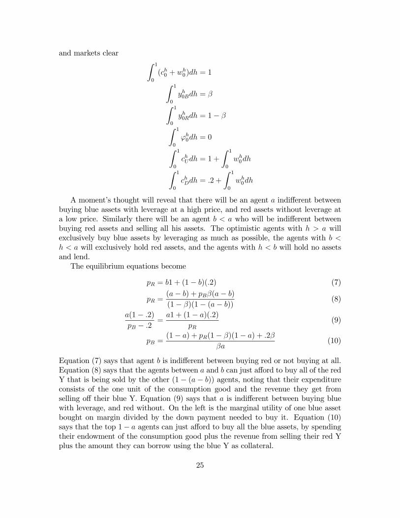
fraction blue 1 0.5 0.05a 0.6861407 0.841775 0.983891b 0.6861407 0.636558 0.600066pred 0.7489125 0.709246 0.680053pblue 0.7489125 0.74684 0.742279

In the table below we describe equilibrium for various values of �Suppose we begin with the situation more or less prevailing six months ago, with

� = 0% and no leverage, just as in our very �rst example where we found the assetspriced at .677. By setting � = 5% and thereby leveraging the 5% new assets (that isturning them into blue assets) the government can raise their price from .677 to .74.Interestingly this also raises the price of the red assets which remain without leverage,from .677 to .680. Providing the same leverage for more assets, by extending � to .5or 1 and thereby leveraging some of the legacy assets, raises the value of all the assets!Thus if one wanted to raise the price of just the 5% new assets, the government shouldleverage all the assets, new and legacy. By holding promises down to .2, there wouldbe no defaults.This analysis holds some lessons for the current discussion about TALF, the gov-

ernment program designed to inject leverage into the economy in 2009. The introduc-tion of leverage for new assets did raise the price of new assets substantially. It alsoraised the price of old assets that were not leveraged (although part of that might bedue to the expectation that the government lending facility will be extended to oldassets as well). One might think that the best way to raise new asset prices is to givethem scarcity value as the only leveraged assets in town. But on the contrary, theanalysis shows that the price of the new assets could be boosted further by extendingleverage to all the legacy assets, without increasing the amount of default.The reason for this paradoxical conclusion is that optimistic buyers always have

the option of buying the legacy assets at low prices. There must be substantialleverage in the new assets to coax them into buying if the new asset prices are muchhigher. By leveraging the legacy assets as well and thus raising the price of thoseassets, the government can undercut the returns from the alternative and increasedemand for the new assets.This analysis also has implications for spillovers from shocks across markets, a

subject we return to later. The loss of leverage in one asset class can depress pricesin another asset class whose leverage remains the same.

2.6 Complete Markets

Suppose there were complete markets, and that agents could trade both Arrow. secu-rities without the need for collateral (assuming everyone keeps every promise). Thedistinctions between red and blue assets would then be irrrelevant. The equilibrium

26

would simply be ((pU ; pD); (xh0 ; wh0 ; x

hU ; x

hD)) such that pU + pD = 1 (so that the con-

stant returns to scale storage earns zero pro�t, assuming the price of c0 is 1) andZ 1

0

(xh0 + wh0 )dh = 1Z 1

0

xhUdh = 1 +

Z 1

0

wh0dhZ 1

0

xhDdh = :2 +

Z 1

0

wh0dh

(xh0 ; wh0 ; x

hU ; x

hD) 2 Bh(p) = f(x0; w0; xU ; xD) :

x0 + pUxU + pDxD � 1 + pU1 + pD(:2)g(x0; w0; xU ; xD) 2 Bh(p)) uh(x0; xU ; xD) � uh(xh0 ; xhU ; xhD)

It is easy to calculate that complete markets equilibrium occurs where (pU ; pD) =(:44; :56) and agents h > :44 spend all of their wealth of 1:55 buying 3.5 units ofconsumption each in state U and nothing else, giving total demand of (1�:44)3:5 = 2:0and the bottom .44 agents spend all their wealth buying 2.78 units of xD each, givingtotal demand of :44(2:78) = 1:2 in total.The price of Y with complete markets is therefore pU1+pD(:2) = :55, much lower

than the incomplete markets, leveraged price of :75. Thus leverage can boost assetprices well above their "e¢ cient" levels.

2.7 CDS and the Repo Market

The collateralized loan markets we have studied so far are similar to the Repo marketsthat have played an important role on Wall Street for decades. In these marketsborrowers take their collateral to a dealer and use that to borrow money via non-contingent promises due one day later. The CDS is a much more recent contract.The invention of the CDS or credit default swap moved the markets closer to

complete. In our two state example with plenty of collateral, their introductionactually does lead to the complete markets solution, despite the need of collateral. Ingeneral, with more perishable goods, and goods in the future that are not tradablenow, the introduction of CDS does not complete the markets.A CDS is a promise to pay the principal default on a bond. Thus thinking of the

asset as paying 1, or .2 if it defaults, the credit default swap would pay .8 in the downstate, and nothing anywhere else. In other words, the CDS is tantamount to tradingthe down Arrow security.The credit default swap needs to be collateralised. There are only two possible

collaterals for it, the security, or the gold. A collateralisable contract promising anArrow security is particularly simple, because it is obvious we need only considerversions in which the collateral exactly covers the promise. So choosing the nor-malizations in the most convenient way, there are essentially two CDS contracts to

27

consider, a CDS promising .2 in state D and nothing else, collateralized by the secu-rity, or a CDS promising 1 in state D, and nothing else, collateralized by a piece ofthe durable consumtion good gold. So we must add these two contracts to the Repocontracts we considered earlier.It is a simple matter to show that the complete markets equilibrium can be im-

plemented via the two CDS contracts. The agents h > :44 buy all the security Y andall the gold, and sell the maximal amount of CDS against all that collateral. Sinceall the goods are durable, this just works out.In this simple model, the CDS is the mirror image of the Repo. By purchasing an

asset using the maximal leverage on the Repo market, the optimist is syntheticallybuying an up Arrow security (on net it pays a positive amount in the up state, andon net it pays nothing in the down state). The CDS is a down Arrow security. It istantamount therefore, to letting the pessimists leverage. That is why the price of theasset goes down once the CDS is introduced.Another interesting consequence is that the CDS kills the repo market. Buyers

of the asset switch from selling repo contracts against the asset to selling CDS. It istrue that since the introduction of CDS in late 2005 into the mortgage market, therepo contracts have steadily declined.In the next section we ignore CDS and reexamine the repo contracts in a dynamic

setting. Then we return to CDS.

3 The Leverage Cycle

If in the two-period example of Section II bad news occurs and the value plummetsin the last period to .2, there will be a crash. This is a crash in the fundamentals.There is nothing the government can do to avoid it. But the economy is far fromthe crash in the starting period. It hasn�t happened yet. The marginal buyer thinksthe chances of a fundamentals crash are only 31%. The average buyer thinks thefundamentals crash will occur with just 15% probability.The point of the leverage cycle is that excess leverage followed by excessive delever-

aging will cause a crash even before there has been a crash in the fundamentals, andeven if there is no subsequent crash in the fundamentals. When the price crasheseverybody will say it has fallen more than their view of the fundamentals warranted.The asset price is excessively high in the initial or over-leveraged normal economy,and after deleveraging, the price is even lower than it would have been at those toughmargin levels had there never been the over-leveraging in the �rst place.

3.1 A Three Period Model

So consider the same example but with three periods instead of two, also taken fromGeanakoplos (2003). Suppose, as before, that each agent begins in state s = 0 withone unit of money and one unit of the asset, and that both are perfectly durable.

28

U

UU

UDDU

DD

D

0

h

1 –h

1 –h

1 –h

h

h 1

1

1

.2

Crash

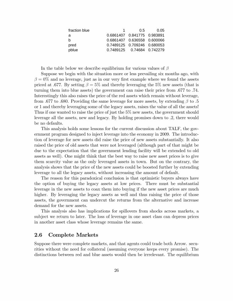
But now suppose the asset Y pays o¤ after two periods instead of one period. Aftergood news in either period, the asset pays 1 at the end. Only with two pieces of badnews does the asset pay .2. The state space is now S = f0; U;D; UU; UD;DU;DDg.We use the notation s� to denote the immediate predecessor of s. Denote by hs theprobability h assigns to nature moving from s� to s: For simplicity we assume thatevery investor regards the U vs D move from period 0 to period 1 as independent andidentically distributed to the U vs D move of nature from period 1 to period 2, andmore particulary hU =

hDU = h.

Diagram 3 hereThis is the situation described in the introduction, in which two things must go

wrong (i.e. two down moves) before there is a crash in fundamentals. Investors di¤erin their probability beliefs over the odds that either bad event happens. The moveof nature from 0 to D lowers the expected payo¤ of the asset Y in every agent�s eyes,and also increases every agent�s view of the variance of the payo¤ of asset Y. Thenews creates more uncertainty, and more disagreement.Suppose agents again have no impatience, but care only about their expected

consumption of dollars. Formally, letting cs be consumption in state s; and letting ehsbe the initial endowment of the consumption good in state s, and letting yh0� be the

29

initial endowment of the asset Y before time begins, we have for all h 2 [0; 1]

uh(c0; cU ; cD; cUU ; cUD; cDU ; cDD)

= c0 + hUcU +

hDcD +

hU

hUUcUU +

hU

hUDcUD +

hD

hDUcDU +

hD

hDDcDD

= c0 + hcU + (1� h)cD + h2cUU + h(1� h)cUD + (1� h)hcDU + (1� h)2cDD(eh0 ; y

h0� ; e

hU ; e

hD; e

hUU ; e

hUD; e

hDU ; e

hDD)

= (1; 1; 0; 0; 0; 0; 0; 0)

We de�ne the dividend of the asset by dUU = dUD = dDU = 1; and dDD = :2; andd0 = dU = dD = 0:The agents are now more optimistic than before, since agent h assigns only a

probability of (1 � h)2 to reaching the only state, DD, where the asset pays o¤ .2.The marginal buyer from before, b = :69, for example, thinks the chances of DD areonly (.31)2 = :09: Agent h = :87 thinks the chances of DD are only (:13)2 = 1:69%:But more importantly, if lenders can lend short term, their loan at 0 will come duebefore the catastrophe can happen. It is thus much safer than a loan at D.

3.2 Equilibrium

Assume that repo loans are one-period loans, so that loan sj promises j in states sUand sD, and requires one unit of Y as collateral. The budget set can now be writteniteratively, for each state s.

Bh(p; �) = f(cs; ys; ('sj)j2J ; ws)s2S 2 (R2+ � RJ � R+)1+S : 8s

(cs + ws � ehs ) + ps(ys � ys�) = ys�ds + ws� +JXj=1

'sj�sj �JXj=1

's�j min(ps + ds; j)

JXj=1

max('sj; 0) � ysg

In each state s the price of consumption is normalized to 1, and the price of theasset is ps and the price of loan sj promising j in states sU and sD is �sj: Agenth spends if he consumes and stores more than his endowment or if he increases hisholdings of the asset. His income is his dividends from last period�s holdings (byconvention dividends in state s go the asset owner in s�) plus what he warehousedfrom last period plus his sales revenue from selling promises, less the payments hemust make on previous loans he took out. Collateral is as always no recourse, so hecan walk away from a loan payment if he is willing to give up his collateral instead.The agents who borrow (taking �sj > 0) must hold the required collateral.The crucial question again is how much leverage will the market allow at each

state s? By the logic we described in the previous section, it can be shown that inevery state s, the only promise that will be actively traded is the one that makes the

30

maximal promise on which there will be no default. Since there will be no default onthis contract, it trades at the riskless rate of interest rs per dollar promised. Using thisinsight we can drastically simplify our notation (as in Fostel-Geanakoplos 2008b) byrede�ning 's as the amount of the consumption good promised at state s for deliveryin the next period, in states sU and sD. The budget set then becomes

Bh(p; r) = f(cs; ys; 's; ws)s2S 2 (R2+ � R� R+)1+S : 8s

(cs + ws � ehs ) + ps(ys � ys�) = ys�ds + ws� +JXj=1

's1

1 + rs� 's�

's � ysmin(psU + dsU ; psD + dsD)g

Equilibrium occurs at prices (p; r) such that when everyone optimizes in his budgetset by choosing (chs ; y

hs ; '

hs ; w

hs )s2S the markets clear in each state sZ 1

0

(chs + whs )dh =

Z 1

0

ehsdh+ ds

Z 1

0

yhs�dhZ 1

0

yhs dh =

Z 1

0

yhs�dhZ 1

0

'hsdh = 0

It will turn out in equilibrium that the interest rate is zero in every state. Thus attime 0, agents can borrow the minimum of the price of Y at U and at D, for everyunit of Y they hold at 0. At U agents can borrow 1 unit of the consumption good, forevery unit of Y they hold at U. At D they can borrow only .2 units of the consumptiongood, for every unit of Y they hold at D. In normal times, at 0, there is not very muchbad that can happen in the short run. Lenders are therefore willing to lend muchmore on the same collateral, and leverage can be quite high. Solving the example asin Section III.D gives the following prices. See Figure 5.

3.3 Crash because of Bad News, De-leveraging, and Bank-rupt Optimists

The price of Y at time 0 of .95 occurs because the marginal buyer is h = :87. Assumingthe price of Y is .69 at D and 1 at U, the most that can be promised at 0 using Y ascollateral is .69. With an interest rate r0 = 0; that means .69 can be borrowed at 0using Y as collateral. Hence the top 13% of buyers at time 0 can collectively borrow.69 (since they will own all the assets), and by adding their own .13 of money theycan spend .82 on buying the .87 units that are sold by the bottom 87%. The price is:95 � :82=:87.Why is there a crash from 0 to D? Well �rst there is bad news. But the bad news

is not nearly as bad as the fall in prices. The marginal buyer of the asset at time 0,

31

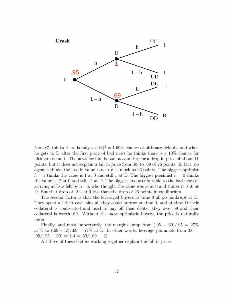
U

UU

UDDU

DD

D

0

h

1 –h

1 –h

1 –h

h

h 1

1

1

R

Crash

.95

.69

1

h = :87, thinks there is only a (.13)2 = 1:69% chance of ultimate default, and whenhe gets to D after the �rst piece of bad news he thinks there is a 13% chance forultimate default. The news for him is bad, accounting for a drop in price of about 11points, but it does not explain a fall in price from .95 to .69 of 26 points. In fact, noagent h thinks the loss in value is nearly as much as 26 points. The biggest optimisth = 1 thinks the value is 1 at 0 and still 1 at D. The biggest pessimist h = 0 thinksthe value is .2 at 0 and still .2 at D. The biggest loss attributable to the bad news ofarriving at D is felt by h=.5, who thought the value was .8 at 0 and thinks it is .6 atD. But that drop of .2 is still less than the drop of 26 points in equilibrium.The second factor is that the leveraged buyers at time 0 all go bankrupt at D.

They spent all their cash plus all they could borrow at time 0, and at time D theircollateral is con�scated and used to pay o¤ their debts: they owe .69 and theircollateral is worth .69. Without the most optimistic buyers, the price is naturallylower.Finally, and most importantly, the margins jump from (:95 � :69)=:95 = 27%

at U to (:69 � :2)=:69 = 71% at D. In other words, leverage plummets from 3:6 =:95=(:95� :69) to 1:4 = :69=(:69� :2).All three of these factors working together explain the fall in price.

32

3.4 Finding the Equilibrium: The Marginal Buyers

To see how to �nd this equilibrium, let b be the marginal buyer in state D and let abe the marginal buyer in state 0: Then we must have

pD = bDU1 +

bDD(:2) � b1 + (1� b)(:2) (11)

pD =(1=a)(a� b) + :2

(1=a)b=1:2a� bb

(12)

a =b(1 + pD)

1:2(13)

p0 =(1� a) + pD

a(14)

a(1� pD)p0 � pD

� aU(1� pD)p0 � pD

= aU1 + aD

aDU bDU

� a1 + (1� a)ab

(15)

a(1� pD)p0 � pD

� aU(1� pD)p0 � pD

= aU1 +

aDpD

aDU bDU

p0�a1 + (1� a)pD ab

p0(16)

Equation (11)says that the price at D is equal to the valuation of the marginalbuyer b at D. Because he is also indi¤erent to borrowing, he will then also be indi¤erentto buying on the margin, as we saw in the collateral section II.C. Equation (12) saysthat the price at D is equal to the ratio of all the money spent on Y at D, divided bythe units sold at D. The top a investors are all out of business at D, so they cannot buyanything. They have spent all their money, and sold all their assets in order to payo¤ their loans at D. Thus the remaining 1� a agents must hold all the consumptiongoods and Y between them, in equal amounts (since they all lent the same amountat 0). Hence at D the remaining investors in the interval [0; a) each own 1=a unitsof Y and have inventoried or collected 1=a dollars. At D the new optimistic buyersin the interval [b; a) spend all they have, which is (1=a)(a � b) dollars plus the :2(1)they can borrow on the entire stock of Y. The amount of Y sold at D is (1=a)b: Thisexplains equation (12). Equation (13) just rearranges the terms in equation (12).Equation (14) is similar to (12). It explains the price of Y at 0 by the amount

spent divided by the amount sold. Notice that at 0 it is possible to borrow pD usingeach unit of Y as collateral. So the top (1� a) agents have (1� a) + pD to spend onthe a units of Y for sale at 0.Equation (15)equates the marginal utility at 0 to a of one dollar, on the right,

with the marginal utility of putting one dollar of cash down on a leveraged purchaseof Y, on the left. The marginal utility of leveraging a dollar by buying Y on marginat time 0 can easily be seen. With p0� pD dollars as downpayment, one gets a payo¤of (1�pD) dollars in state U, to which a assigns probability aU � a; and nets nothingat D, explaining the left hand side of the equation:To see where the right hand side of equation (15) comes from, observe �rst that

agent a can do better by inventorying the dollar (i.e. warehousing the consumption

33

good by taking w0 > 0) at time 0 rather than consuming it. With probablity aU � a;U will be reached and this dollar will be worth one utile. With probability aD � 1�a,D will be reached and a will want to leverage the dollar into as big a purchase of Yas possible. This will result in a gain at D of

a(1� :2)pD � :2

=a(1� :2)

b1 + (1� b)(:2)� :2 =a

b

Hence the marginal utility of a dollar at time 0 is a1 + (1� a)ab; explaining the right

hand side of equation (15):Equation (16) says that a is indi¤erent to buying Y on margin at 0 or buying it

for cash. The right hand side shows that by spending p0 dollars to buy Y at 0, agenta can get a payo¤ of 1 with probability a, and with probability (1� a) a payo¤ of PDdollars at D, which is worth pD ab to a: Equation (16) is a tautological consequence ofthe previous equation. To see this, note that by rewriting equation (15) and usingthe identity �

�=

�implies �

�= �+

�+�we get

a(1� pD)p0 � pD

=pD[a1 + (1� a)ab ]

pD

=a(1� pD) + pD[a1 + (1� a)ab ]

p0 � pD + pD

=a1 + (1� a)pD ab

p0

which is the last equation (16).By guessing a value of b, and then iterating through all the equations, one ends

up with all the variables speci�ed, and a new value of b. By searching for a �xedpoint in b, one quickly comes to the solution just described, with the crash from :95to :69.

3.5 Quantifying the contributions of bad news, deleveraging,and bankruptcy of the optimists

In the crisis of 2007-9 there has been bad news, but according to most �nancialanalysts, the price of assets fell much farther than would have been warranted by thenews. There have been numerous bankruptcies of mortgage companies, and even ofgreat investment banks. And the drop in leverage has been enormous.These kind of events had occured before in 1994 and 1998. The cycle is more

severe this time because the leverage was higher, and the bad news was worse.Of the three symptoms of the leverage cycle collapse, which is playing the biggest

role in our example? This is an easy calculation to make, because we can introduceeach of the three e¤ects on its own into the model and then see how much the price.95 declines.

34

The bad news has the e¤ect of increasing the probability each agent h assigns tothe low payo¤ of .2 at DD from (1�h)2 to (1�h): So we can recalculate equilibriumin the same tree, but with hsD �

p(1� h) > (1 � h) for all s = 0; U;D: The result

is that at node 0 the price is now .79. Thus roughly 60% of the drop in value from.95 to .69 comes from the bad news itself.But that still leaves 40% of the drop explainable only by non-fundamentals (or

technicals as they are sometimes called). We can decompose this 40% into the partthat comes from the bankruptcy and disappearance of the most optimistic buyers,and the rest due to the deleveraging.In the main example, the most optimistic 13% went bankrupt at D. We can isolate

this e¤ect simply by beginning with an economy without these agents. Replacing theset of traders [0; 1] with [0; :87], and therefore the value 1 with .87 in the appropriateequations (12),(13),(14), one can repeat the calculation and �nd that the price at theoriginal node is .89, a drop of 6 points from the original .95, and roughy 20% of theoriginal 26 point drop in the example from 0 to D.In the main example the deleveraging occurred at D when the maximal promise

was reduced to .2. We can simulate the deleveraging e¤ect alone by reducing ourtree to the old one-period model, but replacing the probability of down of 1� h with(1 � h)2: In that new model the equilibrium promise at node 0 will be just .2, butinvestors will still assign the .2 payo¤ probability (1� h)2: This gives an initial pricefor the asset of .89. Thus deleveraging also explains about 20% of the price crash.The roughy linear decomposition of the three factors is due to the linearity of the

beliefs hsU = h; hsD = 1 � h in h: In my 2003 paper I analyzed exactly this samemodel but with more optimistic beliefs because I wanted to avoid this linearity, andalso to illustrate a smaller crash consistent with the minor leverage cycle crash of1998. I assumed hsU = 1 � (1 � h)2; hsD = (1 � h)2; giving probability (1 � h)4 ofreaching DD from 0: In that speci�cation there are many investors with hsU near to1, but once h moves far from 1, the decline in optimism happens faster and faster. Inthat model the price at 0 is p0Y = :99 and the price falls only 12 points to p0D = :87at D. Only the top 6% of investors buy at 0, since they can leverage so much, andthus go bankrupt at D. Without them from the beginning, the price would still be.99, hence the loss of the top tier itself contributes very little. Bad news alone inthat model reduces to the example I have been considering here, which has a startingprice of p0Y = :95:5 Deleveraging alone in that example results in a starting price ofp0Y = :98: Hence the three factors independently add up to much less than the totaldrop. In that example it was the feedback between the three causes that explainedmuch of the drop. In the example in this paper, the total drop is very close to thesum of the parts.

5There was an error in my 2003 paper where I reported that the starting price would be .99 inthe example of this paper (instead of .95).

35

3.6 Conservative optimists

It is very important, and very characteristic of the leverage cycle, that after thecrash, returns are much higher than usual. Survivors of the crash always have greatopportunities. One might well wonder why investors in the example do not foreseethat there might be a crash, and keep their powder dry in cash (or in assets butwithout leverage) at 0, waiting to make a killing if the economy goes to D. Theanswer is that many of them do exactly that.The marginal buyer at 0 is h = :87. He assigns probability 1:69% = (:13)2 to

reaching DD. So he values the asset at 0 at more than .98, yet he he is not rushing tobuy at the price of .95. The reason is that he is precisely looking toward the future.These calculations are embodied in equation (15) of Section III.D. The marginalutility to a of reaching the down state with a dollar of dry powder is not (1 � a),but (1� a)(a=b) precisely because a anticipates that he will have a spectacular grossexpected return of a=b at D.In fact all the investors between .87 and .74 are refraining from buying what they

regard as an underpriced asset at 0, in order to keep their powder dry for the killingat D. If there were only more of them, of course, there would be no crash at D. Butas their numbers rise, so does the price at D, and so their temptation to wait ebbs.It is after all a rare bird who thinks the returns at D are so great, yet thinks Dis su¢ ciently likely to be worth waiting for. This is owing to my assumption thatinvestors who think the �rst piece of bad news is relatively unlikely (high h) alsothink the second piece of bad news is relatively unlikely (high h again) even afterthey see the �rst piece of bad news. This assumption corresponds to my experiencethat hedge fund managers generally are the ones saying things are not that bad, evenafter they start going bad.

3.7 Endogenous Maturity Mismatch

Many authors have lamented the dangers of short term borrowing on long term assets,as we have in this example. It is important to observe that the short term loans Idescribed in the three period model arise endogenously. If long, two period non-contingent loans were also available, then by the previous arguments, since there areonly two outcomes even in the �nal period, the only potentially traded long term loanwould promise .2 in every state. But the borrowers would much prefer to borrow .69on the short term loan. So the long term loans would not be traded.This preference for short term loans is an important feature of real markets.

Lenders know that much less can go wrong in a day than in a year, and so they arewilling to lend much more for a day on the same collateral than they would for a year.Eager borrowers choose the larger quantity of short term loans, and presto, we havean endogenous maturity mismatch. Endogenous collateral can resolve the puzzle ofwhat causes maturity mismatch.

36

3.8 CDS

In my view an important trigger for the collapse of 2007-2009 was the introductionof CDS contracts into the mortgage market in late 2005, at the height of the market.CDS on corporate bonds had been traded for years, but until 2005 there had been nostandardized mortgage CDS contract. I do not know the impetus for this standard-ization; perhaps more people wanted to short the market once it got so high. Butthe implication was that afterward the pessimists, as well as the optimists, had anopportunity to leverage. This was bound to depress mortgage security prices. As Ishow in Section V on the double leverage cycle, this in turn forced underwriters ofmortgage securities to require mortgage loans with higher collateral so they would bemore attractive packages, which in turn made it impossible for homeowners to re�-nance their mortgages, forcing many to default, which then began to depress homeprices, which then made it even harder to sell new mortgages and so on. I believe theintroduction of CDS trading on a grand scale in mortgages is a critical, overlookedfactor in the crisis. Until now people have assumed it all began when home pricesstarted to fall in 2006. But why home prices should begin to fall then has remaineda mystery.To see the e¤ect of introducing a CDS market midstream, suppose in our model

that everyone anticipated correctly that the CDS market would get introduced in themiddle period. Computing equilibrium with repo markets at time 0 and completemarkets from time 1 onwards, we get not just a 26 point drop, but a bigger crash ofpoY = :85 to pDY = :51: The drop becomes an astonishing 34 points, or 40%. If theintroduction of the CDS market occured in the middle period, but was unanticipated,the crash would be even worse. The sudden introduction of CDS in 2005 probablyplayed a bigger role than people realize.Of course if CDS were introduced from the beginning, prices would never have

gotten so high. But they were only introduced after the market was at its peak.

3.9 Complete Markets

The introduction of CDS from the beginning moves the markets close to complete.It is easy to compute the complete markets equilibrium. Nobody would consumeuntil the �nal period, when all the information had been revealed. So we need only�nd four prices of consumption at UU,UD,DU, and DD. The supplies of goods arerespectively 2,2,2,1.2, and the most optimistic people will exclusively consume goodUU, the next most optimistic will exclusively consume UD and so on. The pricesturn out to be pUU = :29; pUD = :16; pDU = :16; pDD = :39: This gives a drop of Yfrom p0Y = :68 to pDY = :43:The complete markets prices are systematically lower than the collateral equilib-

rium, because e¤ectively complete markets amounts to adding the CDS, which meansthe pessimists can leverage as well.With complete markets there is high volatility as well. Indeed the drop in prices

37

from 0 to D is as big as before. With complete markets, the optimists bet on U,selling their wealth at D. The price at D therefore re�ects the opinions of the peoplewho have wealth there, and they are more pessimistic people than at U or 0, andthus we get a big drop in prices at D even with complete markets.The phenomenon of bigger price drops than anybody thinks is justi�ed is thus

consistent with complete markets as well. But I feel it is more likely with incompletemarkets. For example, suppose that we change the beliefs of the agents so that agenth thinks the probability of up is never less than .6, that is suppose

hsU = max(h; :6) for all h and s = 0; D; U

The collateral equilibrium described in the leverage cycle, in which the price of Ydropped from p0Y = :95 to pDY = :69, is absolutely unchanged, since the lowestmarginal buyer was b = :61 at D. The opinions of h < :61 never mattered. On theother hand, the complete markets prices are now p0Y = :87 = (1� (1� :6)2)1 + (1�:6)2(:2) and pDY = :68 = :6(1)+ :4(:2):With complete markets the price drop is only2/3 the size of the collateral equilibrium price drop, and it is completely explainedby the bad news as seen by every agent with h � :6:

3.10 Five Reasons the Leverage Cycle is Bad

The wild gyrations in asset prices as equilibrium leverage ebbs and �ows is alarmingin and of itself. But behind the volatility there are �ve more serious problems.First, very high leverage means that the asset prices are set by a small group of

investors. If agent beliefs are heterogeneous, why should the prices be determinedentirely by the highest outliers? In the model above just the top 13% determined theprice of the asset at date 0. In my 2003 paper, it was just the top 6% who determinedthe price. So few people should not have so much power to determine crucial prices.Leverage allows the few to wield great in�uence.Second, if we add production to the economy, especially of the irreversible kind,

then we would �nd a huge wave of overbuilding. The asset price at 0 is well above thecomplete markets price, because of the expectation by the leveraged few, that goodtimes were coming. In the bad state that overbuilding would need to be dismantledat great cost.Third, asset prices can have a profound e¤ect on economic activity. As Tobin

argued with his concept of Q, when the prices of old assets are high, new productiveactivity, which often involves issuing �nancial assets that are close substitutes for theold assets, is stimulated. When asset prices are low, new activity might grind to ahalt. If we added another group of small business people to the model who did notparticipate in �nancial markets generally, we would �nd that they could easily sellloans at time 0, but would have a hard time at D. Government policy may well havethe goal of protecting these people by smoothing out the leverage cycle. It can easilybe checked that if a regulation were passed that limited promises at date 0 to say

38

.4 (instead of .69), then prices at time 0 would fall from .95 to .91, and prices at Dwould rise from .69 to .70.Fourth, the large �uctuations in asset prices over the leverage cycle lead to massive

redistributions of wealth and changes in inequality. At the beginning everybody hasan equal share of wealth. In the ebullient stage, the optimists become 30% richerthan the pessimists, while in the intermediate down state, the optimists go broke.Inequality becomes extreme in both states.This brings us to the �fth potential cost of too much leverage. Instead of regarding

the optimists as crazy, let us think of them as indispensable to the economy. That isprobably what is meant by the modern term "too big to fail". Geanakoplos-Kubler(2005) shows that if their marginal contribution to society is bigger than what they arepaid, then their bankruptcy results in an externality, since they internalize only theirprivate loss in calculating how much leverage to take on. If in addition the bankruptcyof one optimist makes it more likely in the short run that other optimists will gobankrupt, then the externality can become so big that simply curtailing leverage canmake everybody better o¤.In the next section I drop CDS and return to leveraged loans, but analyze the

more conventional case of common priors and diminishing marginal utility. I �ndthat if some agents get more utility out of holding the collateral than others, thenthe endogenous equilibrium leverage may well involve default. Default can give riseto further ine¢ ciencies, giving us more reasons to monitor and regulate leverage.

4 Heterogeneity based on Utility for Collateral:Endogenous Default

So far we have assumed a continuum of risk neutral agents with identical time dis-counting, who di¤ered in their taste for the collateral on account of their di¤erentpriors about the collateral payo¤s. In this section we introduce an alternative dif-ference, namely that some agents simply enjoy a higher utility from holding thecollateral, such as when they use their houses as collateral. We assume common pri-ors. We �nd once again that there is a unique leverage chosen in equilibrium. Butthis time the leverage is not the maximal amount short of default. On the contrary,we now �nd that the market will select a promise in which there is a great deal ofdefault in the bad state. Worse still, even if both the borrowers and lenders realizethere is a substantial foreclosure cost (to seizing the collateral in case of default), thefree market will still choose promises which allow for a great deal of default.In this model, if we introduce CDS to complete the markets, it turns out that

nobody will trade them. Thus the markets are endogenously incomplete: even ifevery contract can be written, the market will only choose a few because of the needfor collateral.Because we have only two types of agents in this model, equilibrium will not

39

necessarily entail a marginal agent indi¤erent to buying the asset. We shall �nd thatevery buyer of the collateral strictly prefers to buy on margin (i.e. leveraged) tobuying outright. In fact, no agent is willing to buy the collateral with 100% cashdown.

4.1 Example: Borrowing Across Time

We consider an example taken from Geanakoplos (1997) with two kinds of agentsH = fA;Bg, two time periods, and two goods F (food) and H (housing) in eachperiod. For now we shall suppose that there is only one state of nature in the lastperiod.We suppose that food is completely perishable, while housing is perfectly durable.We suppose that agent B likes living in a house much more than agent A,

uA(x0F ; x0H ; x1F ; x1H) = x0F + x0H + x1F + x1H ;

uB(x0F ; x0H ; x1F ; x1H) = 9x0F � 2x20F + 15x0H + x1F + 15x1H :Furthermore, we suppose that the endowments are such that agent B is very poor

in the early period, but wealthy later, while agent A owns the housing stock

eA = (eA0F ; eA0H ; e

A1F ; e

A1H) = (20; 1; 20; 0) ;

eB = (eB0F ; eB0H ; e

B1F ; e

B1H) = (4; 0; 50; 0) :

We suppose that there are contracts (Aj; Cj) with Aj = (j; 0); promising j unitsof food in period 1, and no housing, each collateralized by one house Cj = (0; 1)as before. We introduce a new piece of notation D1j to denote the value of actualdeliveries of asset j at time 1. Given our no recourse collateral, we know D1j =min(jp1F ; p1H):

4.1.1 Arrow�Debreu Equilibrium

If in addition we had a complete set of Arrow securities with in�nite default penaltiesand no collateral requirements, then it is easy to see that there would be a uniqueequilibrium (in prices and utility payo¤s):

p=(p0F ; p0H ; p1F ; p1H) = (1; 30; 1; 15) ;

xA=(xA0F ; xA0H ; x

A1F ; x

A1H) = (22; 0; 48; 0) ;

xB=(xB0F ; xB0H ; x

B1F ; x

B1H) = (2; 1; 22; 1) ;

uA=70 ; uB = 62 :

Assuming that A consumes food in both periods, the price of food would need tobe the same in both periods, since A�s marginal utility for food is the same in both

40

periods. We might as well take those prices to be 1. Assuming that B consumes foodin the last period, the price of every good that B consumes must then be equal toB�s marginal utility for that good. With complete markets, the B agents would beable to borrow as much as they wanted, and they would then have the resources tobid the price of housing up to 30 in period 0 and 15 in period 1.

4.1.2 No Collateral�No contracts Equilibrium

Without the sophisticated �nancial arrangements involved with collateral or defaultpenalties, there would be nothing to induce agents to keep their promises. Recognizingthis, the market would set a price �j = 0 for the contracts. Agents would thereforenot be able to borrow any money. Thus agents of type B, despite their great desireto live in housing, and great wealth in period 1, would not be able to purchase muchhousing in the initial period. Again it is easy to calculate the unique equilibrium:

�j = 0

p = (p0F ; p0H ; p1F ; p1H) = (1; 16; 1; 15) ;

xA = (xA0F ; xA0H ; x

A1F ; x

A1H) =

�20 +

71

32; 1� 71

32 � 16 ; 35�71 � 1532 � 16 ; 0

�;

xB = (xB0F ; xB0H ; x

B1F ; x

B1H) =

�57

32;

71

32 � 16 ; 35 +71 � 1532 � 16 ; 1

�;

uA = 56 ; uB � 64 :

In the �nal period 1, agents of type B are rich and they will bid the house priceup to their marginal utility of 15. Agent A, realizing that he can sell the house for15 in period 1, is e¤ectively paying only 16 � 15 = 1 to have a house in period 0,and is therefore indi¤erent to how much housing he consumes in period 0. Agents oftype B, on the other hand, spend their available wealth at time 0 on housing untiltheir marginal utility of consumption of x0F rises to 30

16, which is the marginal utility

of owning an extra dollar�s worth of housing stock at time 0. That occurs when9� 4xB0F = 30

16, that is, when xB0F =

5732.

4.1.3 Collateral Equilibrium

We now introduce the possibility of collateral, i.e. we suppose the state apparatus issuch that the house is con�scated if payments are not made. The unique equilibrium

41

is then:

Dj = min(j; 15); �j = min(j; 15) ;

p = (p0F ; p0H ; p1F ; p1H) = (1; 18; 1; 15) ;

xA = (xA0F ; xA0H ; x

A1F ; x

A1H) = (23; 0; 35; 0) ;

'A15 = �15 ; 'Aj = 0 for j 6= 15 ;xB = (xB0F ; x

B0H ; x

B1F ; x

B1H) = (1; 1; 35; 1) ;

'B15 = 15 ; 'Bj = 0 for j 6= 15;

uA = 58 ; uB = 72 :

The only contract traded is the one j = 15 that maximizes the promise that will notbe broken. Its price �15 = 15 is given by its marginal utility to its buyer A. AgentB sells the contract, thereby borrowing 15 units of x0F ; and uses the 15 units of x0Fplus 3 he owns himself to buy 1 unit of the house x0H , at a price of p0H = 18: He usesthe house as collateral on the loan, paying o¤ in full the 15 units of x1F in period 1.Since, as borrower, agent B gets to consume the housing services while the house isbeing used as collateral, he gets �nal utility of 72. Agent A sells all his housing stock,since the best he can do after buying it is to live in it for one year, and then sell it ata price of 15 the next year, giving him marginal utility of 16, less than the price of18 (expressed in terms of good F ).The most interesting aspect of the collateral equilibrium is the �rst order condition

for the buyer of collateral. The purpose of collateral is to enable people like B, whodesperately want housing but cannot a¤ord much (for example in the contract lesseconomy), to buy the housing and live in it by borrowing against the future, using thehouse as collateral. To the extent that collateral is not a perfect device for borrowing,one might expect that B does not quite get all the housing he needs, and that themarginal utility of housing might end up greater to B than the marginal utility offood. In fact, the opposite is true.In collateral equilibrium, the marginal utility of a dollar of housing is substantially

less than the marginal utility of a dollar of food

MUBx0Hp0H

=30

18<5

1=MUBx0Fp0F

So why does B buy housing at all? Because he can buy on margin, i.e. with leverage.He needs to pay only 3 = 18 � 15 of cash down for the house, getting 15 utiles inperiod 0, and then he can give the house up in period 1 to repay his loan. Thisleveraged purchase brings 5 utiles per dollar. This is exactly equal to the marginalutility of food per dollar.This is a completely general phenomenon. The leveraged purchase brings more

marginal utility than the straight cash purchase to any buyer who consumes a positive

42

amount at time 0 and is constrained from borrowing as much as he would like by thecollateral requirment.6

4.1.4 Liquidity Wedge and Collateral Value

To the extent that collateral is not perfect in solving the borrowing problem, borrowerswill be constrained from borrowing as much as they would like. The upshot is thatthe marginal utility today of the price of the contracts the borrowers can get byselling is much higher than the marginal utility to them of the deliveries they haveto make: that is what it means for them to be constrained in their selling of loans,i.e., constrained in their borrowing. In Fostel-Geanakoplos (2008b) we called this theliquidity wedge.In the above example, contract j = 15 sells for a price of 15, which gives B

marginal utility at time 0 of (9� 4x0F )15 = 5(15) = 75: The marginal utility of thedeliveries of 15 that B must make at time 1 is (1)(15) = 15: This surplus B gains byborrowing explains why he will choose to sell only the contract j = 15 that maximizesthe amount of money he raises. Selling a contract with j<15 is silly. It deprives B ofthe opportunity to earn more liquidity surplus. Selling contract 16 would not bringany more cash, because contract 16 sells for the same price as contract 15 even thoughit promises more.The collateral has a price of 18 relative to food, which is much too high to be

explained by its utility relative to food. But as explained in Fostel-Geanakoplos(2008b), the price is equal to the payo¤ value plus the collateral value. Housing doesdouble duty. It enables B agents to get utility by living there, but it also enables Bagents to borrow more and to gain more liquidity surplus.

p0H = payo¤ value + collateral value

payo¤ value = (MUBx0H +MUBx1H)=MUBx0Fp0F

= (15 + 15)=5 = 6

collateral value = (MUBx0F�15 �MUBx1FD15)=

MUBx0Fp0F

= (5 � 15� 1 � 15)=5 = 12

p0H = 6 + 12 = 18

4.1.5 The Failure of "E¢ cient Markets"

The e¢ cient markets hypothesis essentially says that prices are priced fairly by themarket, and that even an uninformed agent should not be afraid to trade, becausethe prices already incorporate the information acquired by more sophisticated agents.

6This point is made in Geanakoplos (1997), from where this example is taken. By contrast, inKiyotaki-Moore (1997) the marginal utility of collateral per dollar of its price is higher for its ownerthan the marginal utility per dollar of consumption. But that is only because the collateral ownercannot spend any of his consumption money on the asset.

43

That is true in collateral equilibrium for the contracts, but it is not true of the assetsthat can be used as collateral. An unsophisticated buyer who did not know how touse leverage would �nd that he grossly overpaid for housing.

4.1.6 Optimal Collateral Levels?

What would happen if the government simply refused to let borrowers leverage somuch, say by prohibiting the trade in contracts for j > 14? Although every typeB agent wants to leverage up, using j = 15, when all the other type B agents aredoing the same, he is actually much better o¤ if leverage is limited by government�at. Then everybody will borrow using asset j = 14, and with less buying power, theprice of housing will fall. In fact p0H will fall to 17:05; and the downpayment of 3:05needed to buy the house is therefore barely more than before. (The consumption ofthe B types in period 0 is then a bit smaller than it was, raising the marginal utilityof consumption in period 0. The net utility of buying the house after repaying theloan is now increased from 15 to 15+1=16, so the marginal utility condition continuesto hold.) The big di¤erence is that agent B will only have to deliver 14 in period 1instead of 15. B gains about .7 utiles and A loses about .94 utiles. In short the limiton leverage works out as a transfer from A to B.

4.1.7 Why did Housing Prices Rise so much from 1996-2006?

We can put our last observation more directly. Limits on leverage will reduce collateralgoods prices, and an expansion of leverage will increase their prices. The remarkablerun-up in housing prices in the middle 1990s to the middle 2000s is in my mind lessa matter of irrational exuberance than of leverage.We now consider a more complicated variation of our basic example in which there

is uncertainty and default. Now a higher collateral requirement would mean strictlyless default, but also lower housing prices. So it is interesting to see which collateralrequirement best suits the sellers/lenders.

4.2 Example: Borrowing Across States of Nature, with De-fault

We consider almost the same economy as before, with two agents A and B, and twogoods F (food) and H (housing) in each period. But now we suppose that there aretwo states of nature s = 1 and 2 in period 1, occurring with objective probabilities(1� ") and "; respectively. This example is also taken from Geanakoplos (1997).As before, we suppose that food is completely perishable and housing is perfectly

durable.

44

We assume

uA(x0F ; x0H ; x1F ; x1H ; x2F ; x2H) = x0F + x0H + (1�")(x1F + x1H) + "(x2F + x2H) ;uB(x0F ; x0H ; x1F ; x1H ; x2F ; x2H) = 9x0F � 2x20F + 15x0H + (1�")(x1F + 15x1H) + "(x2F + 15x2H) :

Furthermore, we suppose that

eA = (eA0F ; eA0H ; (e

A1F ; e

A1H); (e

A2F ; e

A2H)) = (20; 1; (20; 0); (20; 0)) ;

eB = (eB0F ; eB0H ; (e

B1F ; e

B1H); (e

B2F ; e

B2H)) = (4; 0; (50; 0); (9; 0)) :

To complete the model, we suppose as before that there are contract promises Ajwith Asj = (j; 0), 8s 2 S promising j units of good F in every state s = 1 and 2,and no housing. We suppose that the collateral requirement for each contract is onehouse Cj = (0; 1), as before.The only di¤erence between this model and the certainty case we had before is

that B is poorer in state 2, and so the housing price must drop in state 2. The �rstquestion is how leveraged will the market allow B to become? Will it allow B todefault?It turns out that it is very easy to calculate the Arrow�Debreu equilibrium and

the collateral equilibrium for arbitrary "; such as " = 1=4. But the no collateralequilibrium is given by a very messy formula, so we content ourselves for that casewith an approximation when " � 0.

4.2.1 Arrow�Debreu Equilibrium

The unique (in utility payo¤s) Arrow�Debreu equilibrium is:

p = ((p0F ; p0H); (p1F ; p1H); (p2F ; p2H)) = ((1; 30); (1�")(1; 15); "(1; 15)) ;

xA = ((xA0F ; xA0H); (x

A1F ; x

A1H); (x

A2F ; x

A2H)) =

�(22; 0);

�20 + 28

(1�") ; 0�; (20; 0)

�;

xB = ((xB0F ; xB0H); (x

B1F ; x

B1H); (x

B2F ; x

B2H)) =

�(2; 1);

�50� 28

1�" ; 1�; (9; 1)

�;

uA = 70; uB = 62� 41" :

Since agent B is so rich in state 1, he sells o¤ enough wealth from there in exchangefor period 0 wealth to bid the price up to his marginal utility of 30. Notice that agentB transfers wealth from state 1 back to period 0, and by holding the house he alsotransfers wealth from state 0 to state 2. With complete markets there is no collapse inhousing prices in state 2, despite the hit the demanders take to their income, becausethose B agents e¤ectively buy insurance against that state.

45

4.2.2 No-Collateral Equilibrium

When " > 0 is very small, we can easily give an approximation to the unique equi-librium with no collateral by starting from the equilibrium in which " = 0.

�j = 0 ;

p = ((p0F ; p0H); (p1F ; p1H); (p2F ; p2H)) =

�(1; 16); (1; 15);

�1;

9

1� 7132�16

��� ((1; 16); (1; 15); (1; 10:4)) ;

xA = ((xA0F ; xA0H); (x

A1F ; x

A1H); (x

A2F ; x

A2H)) �

��20 + 71

32; 1� 71

32�16�;�35� 15�71

32�16 ; 0�; (29; 0)

�;

xB = ((xB0F ; xB0H); (x

B1F ; x

B1H); (x

B2F ; x

B2H)) �

��5732; 7132�16

�;�35 + 15�71

32�16 ; 1�; (0; 1)

�;

uA � 56 ; uB � 64 :

4.2.3 Collateral Equilibrium

We can exactly calculate the unique collateral equilibrium by noting that if B promisesmore in state 2 than the house is worth, then he will default and the house will becon�scated. But after all the agents of type B default in state 2, they will spend allof their endowment eB2F on good 2H, giving a price p2H = 9. Perhaps surprisingly theequilibrium described below con�rms that the B agents do choose to promise morethan they can pay in state 2, and the A agents knowingly buy those promises. Indeedthe same contract j = 15 is traded as when there was certainty and no default. Itsprice is �15 = (1�")15 + "9 because the rational A agents pay less, anticipating thedefault in state 2.

D1j = min(j; 15); D2j = min(j; 9); �j = (1�")D1j + "D2j ;

((p0F ; p0H); (p1F ; p1H); (p2F ; p2H)) = ((1; 3 +�15); (1; 15); (1; 9)) ;

xA = ((xA0F ; xA0H); (x

A1F ; x

A1H); (x

A2F ; x

A2H)) = ((23; 0); (35; 0); (29; 0)) ;

'A15 = �15 ; 'Aj = 0 for j 6= 15 ;'B15 = 15 ; '

Bj = 0 for j 6= 15 ;

xB = ((xB0F ; xB0H); (x

B1F ; x

B1H); (x

B2F ; x

B2H)) = ((1; 1); (35; 1); (0; 1))

At the equilibrium prices, each agent of type A is just indi¤erent to buying or notbuying any contract. At these prices any agent of type B reasons exactly as before.Since money is so much more valuable to him at time 0 than it is in the future, hewill borrow as much as he can, even if it leads to default in state 2. He will onlytrade contract j = 15. Notice that the amount of default in the bad state, and theequilibrium downpayment of 3 on the house, do not depend on the probability 1� "of the good state.Thus we see that the free market will not choose levels of collateral which eliminate

default. We are left to wonder whether the collateral levels are in any sense optimalfor the economy: does the free market arrange for the optimal amount of default?

46

4.2.4 Excess Volatility

Since the 1929 stock market crash it has been widely argued that low margin re-quirements can increase the volatility of stock prices. The argument is usually of thefollowing kind: when there is bad news about the stocks, margins are called and theagents who borrowed against the stocks are forced to put them on the market, whichlowers their prices still further.The trouble with this argument is that it does not quite go far enough. In general

equilibrium theory, every asset and commodity is for sale at every moment. Hencethe crucial step in which the borrowers are forced to put the collateral up for sale hasby itself no bite. On the other hand the argument is exactly on the right track.We argued that using houses or stocks, or mortgage derivatives as collateral for

loans (i.e., allowing them to be bought on margin) makes their prices more volatile.The reason is that those agents with the most optimistic view of the assets�futurevalues, or simply the highest marginal utility for their services, will be enabled bybuying on margin to hold a larger fraction of them than they could have a¤ordedotherwise. But with bad news for the asset, there is a redistribution of wealth awayfrom the optimists and toward the pessimists who did not buy on margin. Themarginal buyer of the stock is therefore likely to be someone less optimistic or lessrich than would have been the case had the stock not been purchased on margin, andthe income redistribution not been so severe. Thus the fall in price is likely to bemore severe than if the stock could not have been purchased on margin.Our story is borne out vividly in the example when di¤erences stem not from

optimism but from heterogeneous tastes for housing. When the housing stock canbe purchased on margin (i.e., used as collateral), agents of type B are enabled topurchase the entire housing stock, raising its price from 16 (where it would have beenwithout collateral) to 18. In the bad state these agents default and all their holdingsof the housing stock are seized. Although they end up buying back the entire housingstock, their wealth is so depleted that they can only bid up the housing prices to 9.When there is no collateral the agents of type B can a¤ord to purchase only a

fraction � = 71=(32)(16) of the housing stock at time 0 (if " is very small). But theyown that share free and clear of any debts. Thus when bad news comes, they do notlose anything. They can apply their wealth to purchasing the remaining 1�� of thehousing stock, which forces the price up to approximately 10.4. Thus when there isno leverage, the housing prices are never as high nor never as low as when the housingstock can be used as collateral. When markets are complete, the housing price is 15at both states, una¤ected by the shock to the wealth of B agents.

4.2.5 Endogenous Incomplete Markets

Until now we have assumed that markets were incomplete, restricting contracts topromises that were non-contingent, and then �nding the endogenous leverage. Sup-pose a contingent contract were o¤ered that paid only in the down state, using the

47

house as collateral. (Or paid only in the up state). It is evident that if such a contractcould be traded, and if delivery were enforced by harsh penalties, then there wouldbe Pareto gains to be made. Either contingent contract, together with the risklesspromise, would create full spanning. But if contracts could only be enforced withcollateral, would either contingent contract be traded? The answer is no! Such acontract wastes collateral, which is in very short supply, because it does not use thecollateral value of the house in the other state. A moment�s re�ection should convincethe reader that no matter what contract is o¤ered, the only ones that will be tradedwould be those that promised more than the full value of the house in every state.This stands in contrast to the example in Section II where the collateral would beplentiful enough to support trade in Arrow securities if they were introduced.Of course the situation would be quite di¤erent if the same house could back

multiple promises, one paying o¤ exclusively in the �rst state and the other payingo¤ exclusively in the second state. That kind of tranching would lead to spanning.(But not necessarily to the complete markets solution, since the amount of promiseswould still be limited by the collateral.) In practice one piece of collateral rarelyhas several anti-correlated loans written on it; tranching like that occurs only on bigpools of assets. One house might have two mortgages written on it, but in the goodstates they both deliver in full, and in the bad states they are both compromised.What is interesting here is that the scarcity of collateral does not ration trade

equally in all contracts, say reducing trade in each Arrow security by 40%. Insteadit shuts down trade altogether in many contracts (here in both Arrow securities)and concentrates it all in a di¤erent, less felicitous, but more collateral economizing,contract.

4.2.6 Ine¢ ciency and Government Intervention

Ine¢ ciency arises in these models from sources apart from over-leveraging. First,promises only come in limited forms (like the non-contingent promises we have mostlyassumed), preventing some kinds of insurance from being traded. In our example (orin a slight modi�cation of it such as we shall shortly consider), agents of type Bmight want to buy insurance that pays o¤ in state 2 from agents of type A. But ifall contracts are non-contingent, that insurance is not available. Second, even if thepromises could come in any form, their quantity and form are limited by the scarcityof collateral, as we saw in the last section. The scarcity of collateral will often shutdown many �nancial markets altogether, including the insurance market for state2. This gives a compelling reason for the government to provide that insurance,e¤ectively bailing people out in the down state.The government can always �nd some intervention to compensate for the missing

markets or the collateral constraints to make everybody better o¤. For example, atransfer to every agent at time 0 who begins the period without a house, coupledwith a transfer to every agent who begins a state in period 1 without a house, would

48

make everyone better o¤. These transfers together simply amount to a loan from A toB: the private sector cannot manage to reproduce these additional transfers becausethere is not enough collateral.But in keeping with the subject of this paper, I shall ignore these interventions

and con�ne my attention to the e¢ cacy of regulating leverage. In the section onheterogeneous priors we found �ve reasons why there might be excessive leverage.But in that model there was no default. When there is heterogeneous utility forholding collateral, we found that default naturally arises in equilibrium, if marketsare incomplete. This gives rise to another three dangers from excessive leverage, inaddition to the �ve discussed earlier.A sixth source is debt overhang (see Myers 1977). In our example, agents of type

B and A will agree to trade loans that promise 15 in both states in period 1, as wesaw. Imagine now that B had an opportunity to invest � units of food-equivalent attime 0 to increase the size of his house by �% at time 1. The expected revenue thisbrings is (1 � ")15�% + "9�%: However, if B tries to raise this money by issuingnew debt that is junior to the debt already issued, he can only deliver (1� ")15�%because the revenue in the second state will go to the old bondholders. Even if thenew debt is of equal seniority to the old debt, it will be heavily diluted in the secondstate. So if (1� ")15�%+ "9�% > � > (1� ")15�%; an e¢ cient investment will notbe made. There is no investment in the current model, but we return to this problemin two sections.A seventh source of ine¢ ciency is the cost of seizing collateral, which until now

we have taken to be zero. We discuss this in detail in the next section.I conclude with an eighth problem that that also could sometimes be helped

by limiting leverage, whether or not there is default. When markets are incomplete,Geanakoplos-Polemarchakis (1986) showed that generically there is an intervention attime 0 alone that can lead to a Pareto improvement by changing the asset ownershipstructure. When markets reclear in period 1 the new distribution of assets leads toa change in prices which itself redistributes wealth across states in a way that wasnot spanned by the asset payo¤s. In the example of this Section, the type B agentswould like to buy insurance for state 2, but cannot.In the example as it stands, curtailing leverage does not help, because it does not

change prices in period 1. In particular, prohibiting contracts j > 14 would not bePareto improving. In the new equilibrium only contract j = 14 would be traded, butthe price of housing in states 1 and 2 would remain at 15 and 9, respectively.But one could imagine a variant of the example, obtained partly by making the

utilities strictly concave, such that a limit on leverage would change prices in a helpfuldirection. With less borrowing, B would be richer in period 1. This would turn pricesagainst B in state 1 where B was already rich and buying. But it would turn pricesin B�s favor in state 2 where he had been a forced seller that now can sell less. Theseprice changes have the same e¤ect as the missing insurance contract, which transferswealth from B to A in state 1, and from A to B in state 2. That is the key idea to

49

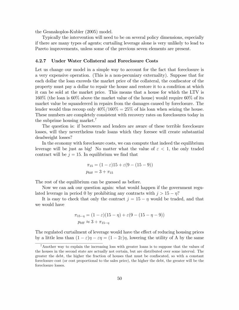
the Geanakoplos-Kubler (2005) model.Typically the intervention will need to be on several policy dimensions, especially

if there are many types of agents; curtailing leverage alone is very unlikely to lead toPareto improvements, unless some of the previous seven elements are present.

4.2.7 Under Water Collateral and Foreclosure Costs

Let us change our model in a simple way to account for the fact that foreclosure isa very expensive operation. (This is a non-pecuniary externality). Suppose that foreach dollar the loan exceeds the market price of the collateral, the con�scator of theproperty must pay a dollar to repair the house and restore it to a condition at whichit can be sold at the market price. This means that a house for which the LTV is160% (the loan is 60% above the market value of the house) would require 60% of itsmarket value be squandererd in repairs from the damages caused by foreclosure. Thelender would thus recoup only 40%=160% = 25% of his loan when seizing the house.These numbers are completely consistent with recovery rates on foreclosures today inthe subprime housing market.7

The question is: if borrowers and lenders are aware of these terrible foreclosurelosses, will they nevertheless trade loans which they foresee will create substantialdeadweight losses?In the economy with foreclosure costs, we can compute that indeed the equilibrium

leverage will be just as big! No matter what the value of " < 1; the only tradedcontract will be j = 15: In equilibrium we �nd that

�15 = (1� ")15 + "(9� (15� 9))p0H = 3 + �15

The rest of the equilibrium can be guessed as before.Now we can ask our question again: what would happen if the government regu-

lated leverage in period 0 by prohibiting any contracts with j > 15� �?It is easy to check that only the contract j = 15 � � would be traded, and that

we would have

�15�� = (1� ")(15� �) + "(9� (15� � � 9))p0H � 3 + �15��

The regulated curtailment of leverage would have the e¤ect of reducing housing pricesby a little less than (1� ")� � "� = (1� 2")�; lowering the utility of A by the same

7Another way to explain the increasing loss with greater loans is to suppose that the values ofthe houses in the second state are actually not certain, but are distributed over some interval. Thegreater the debt, the higher the fraction of houses that must be con�scated, so with a constantforeclosure cost (or cost proportional to the sales price), the higher the debt, the greater will be theforeclosure losses.

50

amount. The utility of B would rise by (1 � ")�, this time giving an increase in thesum of utilities. Curtailing leverage is now bene�cial, provided the probability ofdown is not too low, because this lowers the deadweight loss in the down state. Theindividual agents will not curtail leverage themselves, even though they internalizethe externality, because the borrowers are so desperate to borrow money. What theydon�t realize is that if all of them borrowed less, the price of housing at time 0 wouldfall and so they would not lose much by borrowing less, yet would still avoid thedeadweight loss in the bad state.There is a limit on how big � can be, however, because if 3 + �15�� falls below

1 + (1� ")15 + "9; then the type A agents will buy the house at time 0.In the next section, however, we see that there is lots of room to curtail leverage.When there are foreclosure costs, the equilibrium contract described in Section

V.B.6, where agents had the freedom to design contracts with any promises theyliked, would change. Now the mortgage payment due would be indexed to the priceof housing. That way the lender could avoid the foreclosure costs, which are based onthe how far under water the house becomes. In the real world we do not yet see suchcontracts. The real world seems closer to the situation we described in all the othersections, outside of V.B.6, in which promises are non-contingent by assumption.

5 The Double Leverage Cycle

5.1 Mortgages and Repos

By combining the two main models from the last sections, I build a model of thedouble leverage cycle that allows us to see all eight of the potential pitfalls of leverage.One of the main causes of the severity of the current leverage cycle is that there are twoof them, in the housing market via mortgages and in the mortgage securities marketvia the repo market, and the two reinforce each other in a destructive feedback.Houses back mortgage securities, hence a crash in housing prices has rami�cationsfor the securities market. But a crash in the price of mortgage securities a¤ects theloans homeowners can get, which in turn a¤ects the housing market. One minor twistto the models is that I assume houses must be constructed.So consider now a population made up of the type B homeowners from the model

of Section IV, who get utility from living in houses as well as from consumption,and the investors h 2 [0; 1] from the model of Section III, who only get utility fromconsumption. The homeowners will issue long maturity mortgages in order to borrowthe money to build their houses, using the houses as collateral. As in the model ofSection IV, these mortgages will be endogenously chosen in equilibrium at levels thatlead to default when the houses lose too much value. We suppose as in Section IV thatthere is a substantial foreclosure loss. It will turn out that the mortgage has payo¤sexactly like the payo¤s from the Y security in our �rst model. These mortgages willbe packaged and sold to the optimists h 2 [:87; 1] who �gure the state is very likely

51

to be a good state in which the houses are valuable and the mortgages pay o¤ infull. The optimists will borrow the money to buy the mortgages from the pessimistsh 2 [0; :87) in the short maturity repo market, using the mortgages as collateral fortheir loans. The houses thus serve twice as collateral, �rst backing the homeownermortgage loans, and then backing the mortgage securities which back the optimists�repo borrowing.More concretely, let us consider an economy with 3 time periods 0,1,2, and states

of the world 0,U,D,UU,UD,DU,DD, as in Section III. In addition to the durableconsumption good, which we now call canned food, and housing, there is also a laborgood to enable the building of the houses. We use the letter F to describe the cannedfood, H for housing, and L to denote leisure. Suppose there is a constant-returns-to-scale production technology that is owned by a pro�t maximizing entrepreneur andthat can take 18.5 units of labor at time 0 and transform them into a house at time0 (that will then be perfectly durable). Canned food can be eaten at any time, butis durable. Housing can be enjoyed with no diminution to its quantity.Let there be a continuum of type B agents who each begin with 1 unit of canned

food and 3.15 units of labor, and no houses at time 0, and 50 units of canned foodin UU,UD,DU, and 9 units of canned food in DD, and no other endowments. Thisis exactly like the model of Section IV, except that we stretch out the model tothree periods by inserting another period in the middle. Let type B agents assignprobability (1�") to nature moving up at any state, and suppose the marginal utilityof leisure (that is, the marginal disutility of labor) is denoted by c. Let their utilitybe

uB(x0F ; x0H ; x0L; xUUF ; xUUH ; xUDF ; xUDH ; xDUF ; xDUH ; xDDF ; xDDH ; )

= 9x20F � 2x20F + 15x0H + cx0L + (1� ")2(xUUF + 15xUUH)+(1� ")"(xUDF + 15xUDH) + "(1� ")(xDUF + 15xDUH) + "2(xDDF + 15xDDH)

((eB0F ; eB0H ; e

B0L); (e

BUUF ; e

BUDF ; e

BDUF ; e

BDDF ))

= ((1; 0; 3:15); (50; 50; 50; 9))

Suppose also there is a continuum of agents h 2 [0; 1] who are exactly like theagents in our �rst model, except that instead of owning one unit of X and Y at time0, they each own 15 units of food and 15 hours of labor at time 0. Agent h 2 [0; 1]has utility and endowments

uh(x0F ; x0L; x0L; xUF ; xDF ; xUUF ; xUDF ; xDUF ; xDDF )

= x0F + �cx0L + hxUF + (1� h)xDF+ h2xUUF + h(1� h)xUDF + (1� h)hxDUF + (1� h)2xDDF

(eh0F ; eh0H ; e

h0L) = (15; 0; 15)

52

These agents also have a disutility of work �c: If c or �c falls below the ratio of wages tothe price of food, then the type B agents or the heterogeneous agents h 2 [0; 1] willstop working.The contracts in the economy are of two types, depending on the collateral. In

one kind of contract j, called a mortgage loan of type j, agents at time 0 can makea long term promise of the �xed amount j of good F in every one of the last statesUU,UD,DU,DD, using one house as collateral. In the other type of contract (s; k; j)called a Repo, agents at node s can make a short term promise of k units of good Fin every immediate successor state of node s, using mortgage contract j as collateral.In our economy, the type B agents will borrow money at time 0 by issuing the

mortgage j=15, using the house they will be constructing at the same time as collat-eral. The most optimistic agents in [0,1] will buy those mortgages, thereby lendingthe B agents the money. Since the mortgages will default in state DD (but not untilthen), they will be risky. Hence the pessimists will not want to buy those mortgages,and the optimists don�t have enough money to buy them all. So they will borrowmoney from the pessimists by selling repo loans against the mortgages they hold.These safer repo loans will be held by the pessimists. The Repos are one-periodloans, unlike the mortgage, which is a two-period loan.8

Let us make the hypothesis that if the house is underwater by y dollars when theloan comes due, then y dollars must be wasted in order to restore the house to mintcondition to sell on a par with the other houses on the market. In all the terminalstates except DD, the houses will not be underwater, and the house will sell for 15.But in DD the house will only sell for 9, which means it will be underwater with amortgage promise of 15, so the mortgage will only deliver 9-(15-9)=3 to the mortgageholder after he con�scates the house and sells it, net of the restoration costs.We see that the terminal payo¤s of the mortgage security are (15,15,15,3), which

is tantamount to 15 units of the security Y from our �rst example. The agents oftype h each own 15 units of the canned food, exactly 15 times what they owned of thedurable consumption good before, and their labor income is exactly enough to buyone mortgage security, again 15 times as valuable as the security in our �rst example.Hence this equilibrium we are computing is just the one in our �rst example scaledup by a factor of 15.In view of our earlier analysis, equilibrium is easy to describe. We normalize

by taking the price of canned food to be 1 in every state. In equilibrium the priceof labor in period 0 will be :95. The income of the B agents at time 0 is then1 + (3:15)(:95) = 4. By constant returns to scale, the price of the house will thenbe (18:15)(:95) = (3:15 + 15)(:95) = 3 + 14:25 = 17:25. The B agents will each buya house by putting 3 dollars down and borrowing the remaining 14.25 by issuing a

8It can be shown that if short term mortgages were o¤ered, they would not be traded. Sincethere is a large foreclosure loss from default, and since the equilibrium mortgage involves default, itis not in the interest of borrower and lender to have short term mortgages. Thus the mortgages areendogenously long term loans, and the repos are endogenously short term loans

53

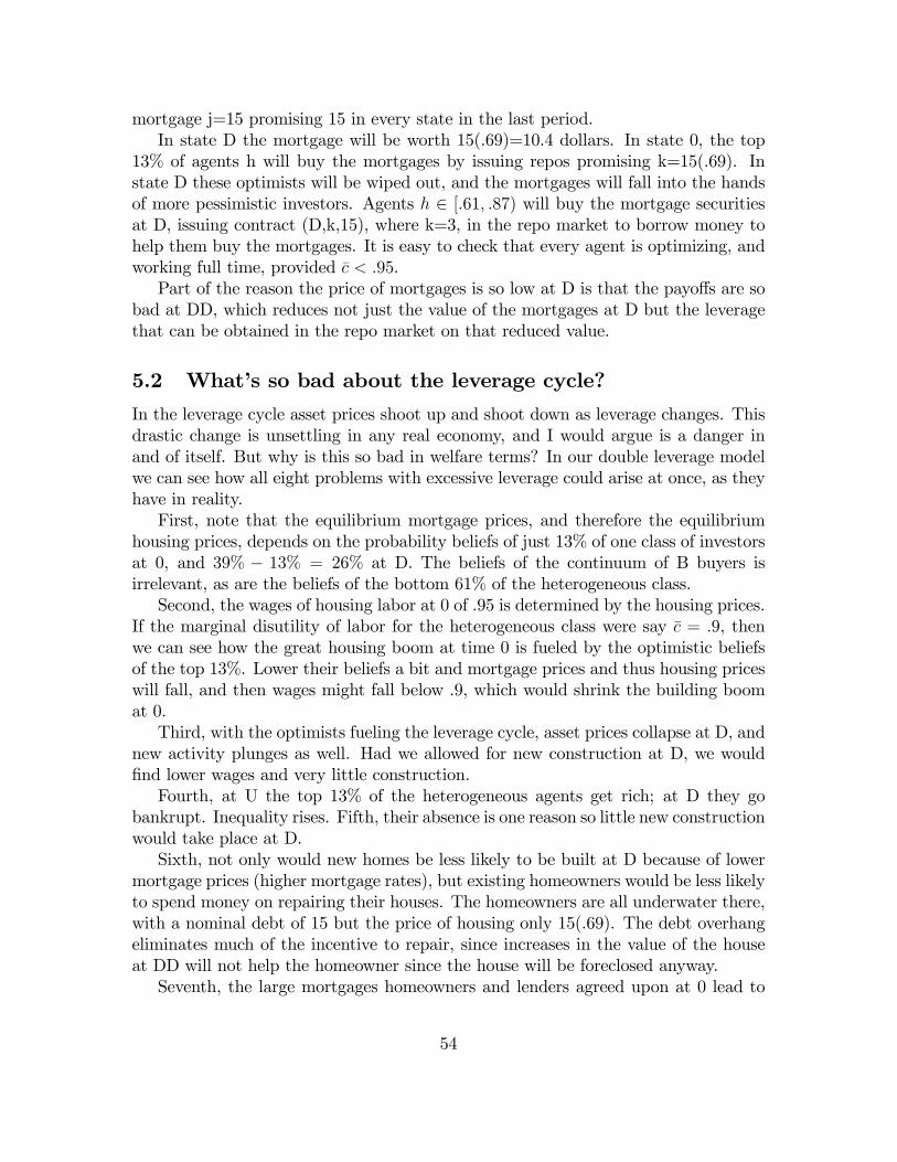
mortgage j=15 promising 15 in every state in the last period.In state D the mortgage will be worth 15(.69)=10.4 dollars. In state 0, the top

13% of agents h will buy the mortgages by issuing repos promising k=15(.69). Instate D these optimists will be wiped out, and the mortgages will fall into the handsof more pessimistic investors. Agents h 2 [:61; :87) will buy the mortgage securitiesat D, issuing contract (D,k,15), where k=3, in the repo market to borrow money tohelp them buy the mortgages. It is easy to check that every agent is optimizing, andworking full time, provided �c < :95.Part of the reason the price of mortgages is so low at D is that the payo¤s are so

bad at DD, which reduces not just the value of the mortgages at D but the leveragethat can be obtained in the repo market on that reduced value.

5.2 What�s so bad about the leverage cycle?

In the leverage cycle asset prices shoot up and shoot down as leverage changes. Thisdrastic change is unsettling in any real economy, and I would argue is a danger inand of itself. But why is this so bad in welfare terms? In our double leverage modelwe can see how all eight problems with excessive leverage could arise at once, as theyhave in reality.First, note that the equilibrium mortgage prices, and therefore the equilibrium

housing prices, depends on the probability beliefs of just 13% of one class of investorsat 0, and 39% � 13% = 26% at D. The beliefs of the continuum of B buyers isirrelevant, as are the beliefs of the bottom 61% of the heterogeneous class.Second, the wages of housing labor at 0 of .95 is determined by the housing prices.

If the marginal disutility of labor for the heterogeneous class were say �c = :9, thenwe can see how the great housing boom at time 0 is fueled by the optimistic beliefsof the top 13%. Lower their beliefs a bit and mortgage prices and thus housing priceswill fall, and then wages might fall below .9, which would shrink the building boomat 0.Third, with the optimists fueling the leverage cycle, asset prices collapse at D, and

new activity plunges as well. Had we allowed for new construction at D, we would�nd lower wages and very little construction.Fourth, at U the top 13% of the heterogeneous agents get rich; at D they go

bankrupt. Inequality rises. Fifth, their absence is one reason so little new constructionwould take place at D.Sixth, not only would new homes be less likely to be built at D because of lower

mortgage prices (higher mortgage rates), but existing homeowners would be less likelyto spend money on repairing their houses. The homeowners are all underwater there,with a nominal debt of 15 but the price of housing only 15(.69). The debt overhangeliminates much of the incentive to repair, since increases in the value of the houseat DD will not help the homeowner since the house will be foreclosed anyway.Seventh, the large mortgages homeowners and lenders agreed upon at 0 lead to

54

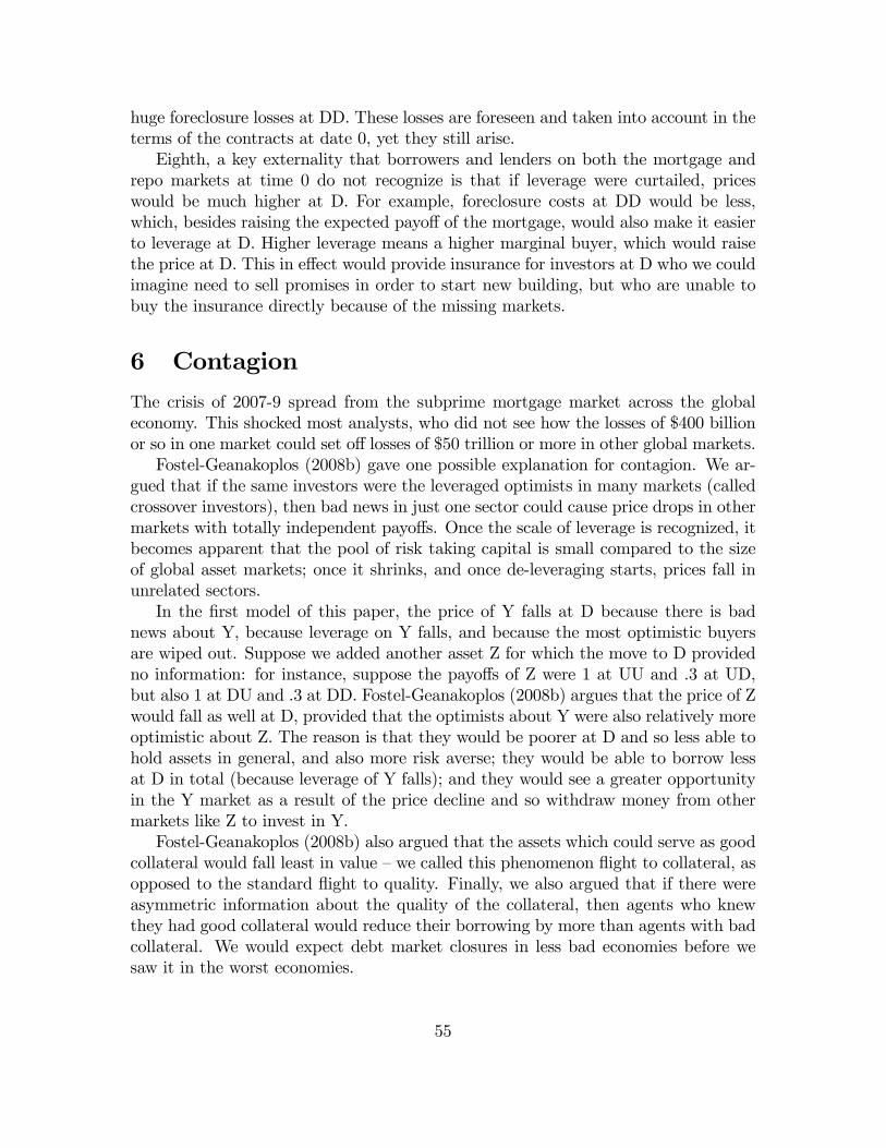
huge foreclosure losses at DD. These losses are foreseen and taken into account in theterms of the contracts at date 0, yet they still arise.Eighth, a key externality that borrowers and lenders on both the mortgage and

repo markets at time 0 do not recognize is that if leverage were curtailed, priceswould be much higher at D. For example, foreclosure costs at DD would be less,which, besides raising the expected payo¤ of the mortgage, would also make it easierto leverage at D. Higher leverage means a higher marginal buyer, which would raisethe price at D. This in e¤ect would provide insurance for investors at D who we couldimagine need to sell promises in order to start new building, but who are unable tobuy the insurance directly because of the missing markets.

6 Contagion

The crisis of 2007-9 spread from the subprime mortgage market across the globaleconomy. This shocked most analysts, who did not see how the losses of $400 billionor so in one market could set o¤ losses of $50 trillion or more in other global markets.Fostel-Geanakoplos (2008b) gave one possible explanation for contagion. We ar-

gued that if the same investors were the leveraged optimists in many markets (calledcrossover investors), then bad news in just one sector could cause price drops in othermarkets with totally independent payo¤s. Once the scale of leverage is recognized, itbecomes apparent that the pool of risk taking capital is small compared to the sizeof global asset markets; once it shrinks, and once de-leveraging starts, prices fall inunrelated sectors.In the �rst model of this paper, the price of Y falls at D because there is bad

news about Y, because leverage on Y falls, and because the most optimistic buyersare wiped out. Suppose we added another asset Z for which the move to D providedno information: for instance, suppose the payo¤s of Z were 1 at UU and .3 at UD,but also 1 at DU and .3 at DD. Fostel-Geanakoplos (2008b) argues that the price of Zwould fall as well at D, provided that the optimists about Y were also relatively moreoptimistic about Z. The reason is that they would be poorer at D and so less able tohold assets in general, and also more risk averse; they would be able to borrow lessat D in total (because leverage of Y falls); and they would see a greater opportunityin the Y market as a result of the price decline and so withdraw money from othermarkets like Z to invest in Y.Fostel-Geanakoplos (2008b) also argued that the assets which could serve as good

collateral would fall least in value �we called this phenomenon �ight to collateral, asopposed to the standard �ight to quality. Finally, we also argued that if there wereasymmetric information about the quality of the collateral, then agents who knewthey had good collateral would reduce their borrowing by more than agents with badcollateral. We would expect debt market closures in less bad economies before wesaw it in the worst economies.

55

7 References

Adrian, Tobias, and Hyun Shin �Liquidity and Leverage�. 2009. Forthcoming in theJournal of Financial IntermediationBernanke, Ben, Mark Gertler and Simon Gilchrist. 1996. �The Financial Accela-

tor and the Flight to Quality.�Review of Economics and Statistics, 78(1): 1�15.Bernanke, Ben, Mark Gertler and Simon Gilchrist. 1999. "The Financial Accel-

erator in a Quantitative Business Cycle Framework", pp 1341-1393 in Handbook ofMaroeconomics, Volume 1, ed by J.B. Tayolor and M. Woodford, Elsevier.Brunnermeier, Markus, and Llasse Pedersen 2009. �Market Liquidity and Funding

Liquidity.�Review of Financial Studies, vol 22,6,2201-2238.Caballero, Richardo J., and Arvind Krishnamurthy. 2001. �International and

Domestic Collateral Constraints in a Model of Emerging Market Crises.�Journal ofMonetary Economics, 48(3): 513�48.Fostel, Ana, and John Geanakoplos. 2008. �Collateral Restrictions and Liquidity

under-Supply: A Simple Model.�Economic Theory, 35(3): 441�67.Fostel Ana, and John Geanakoplos. 2008. �Leverage Cycles and the Anxious

Economy�American Economic Review 2008, 98:4, 1211-1244.Geanakoplos, John. 1997. �Promises, Promises.�In The Economy as an Evolving

Complex System II, ed. W. Brian Arthur, Steven Durlauf, and David Lane, 285�320.Reading, MA: Addison-Wesley.Geanakoplos, John. 2003. �Liquidity, Default, and Crashes: Endogenous Con-

tracts in General Equilibrium.�In Advances in Economics and Econometrics: Theoryand Applications, Eighth World Conference,Vol. 2, 170�205. Econometric SocietyMonographs.Geanakoplos, John and Herakles Polemarchakis 1986. "Existence, Regularity,

and Constrained Suboptimality of Competitive Allocations when the Asset Marketis Incomplete" in Uncertainty, Information, and Communication, Essays in Honorof Ken Arrow, edited by W. Heller, R. Starr, and D. Starrett, 65-96, Cambridge,Cambridge University Press, 1986.Geanakoplos, John and Felix Kubler 2005. "Leverage, Incomplete Markets, and

Pareto Improving Regulation", unpublished.Geanakoplos, John and William Zame (2009). "Collateralized Security Markets",

unpublished. Earlier versions 1997, 2002, 2005.Gromb, Denis and Vayanos, Dimitri, 2002. "Equilibrium and welfare in markets

with �nancially consrained arbitrageurs" 66,361-407.Harrison, J. Michael and David M. Kreps "Martingales and Arbitrage in Multi-

period Securities Markets", Journal of Economic Theory, 20, 381-408.Holmstrom, Bengt and Jean Tirole, 1997. �Financial Intermediation, Loanable

Funds, and the Real Sector,�Quarterly Journal of Economics, 112, 663-692.Kiyotaki, Nobuhiro, and John Moore. 1997. �Credit Cycles.�Journal of Political

Economy, 105(2): 211�48.

56

Lorenzoni, Guido (2008). "Ine¢ cient Credit Booms". Review of Economic Stud-ies, 75,3,809-833.Minsky, Hyman 1986. Stabilizing an Unstable Economy. Yale University Press,

New Haven.Myers, Stewart. 1977. "Determinants of Corporate Borrowing" Journal of Finan-

cial Economics, 5, 147-176.Tobin, James and Stephen Golub 1998Money, Credit, and Capital. Irwin/McGraw-

Hill.

57