THE LEVEL CROSSING PROBLEM IN

SEMI-CLASSICAL ANALYSIS

I. The symmetric case

(to appear in the Proceedings of

Frederic Pham’s congress)

Yves Colin de Verdiere

September 24, 2002

Prepublication de l’Institut Fourier n0 574 (2002)http://www-fourier.ujf-grenoble.fr/prepublications.html

Institut Fourier, Unite mixte de recherche CNRS-UJF 5582

BP 74, 38402-Saint Martin d’Heres Cedex (France)

yves.colin-de-verdiere@ujf-grenoble.fr

http://www-fourier.ujf-grenoble.fr/˜ycolver/

Abstract

Our goal is to recover and extend the difficult results of George Hage-dorn (1994) on the propagation of coherent states in the Born-Oppenheimerapproximation in the case of generic crossings of eigenvalues of the (matrixvalued) classical Hamiltonian. This problem, going back to Landau and Zenerin the thirties, is often called the “Mode Conversion Problem” by physicistsand occurs in many domains of physics (see the paper [23] by W. Flynn andR. Littlejohn).

We want to obtain a geometrical description of the propagation of states inthe framework of semi-classical analysis and WKB-Lagrangian states. It turnsout that, in the very beautiful (but not well known!) paper [7] published in1993, Peter Braam and Hans Duistermaat found that there is a formal normalform for this problem. A formal normal form for the dispersion relation werealready founded by Arnold [3]. In our paper, we show, using Nelson’s waveoperators method, that, in the hyperbolic case, their normal form can beextended to a local normal form in the phase space.

Then, we extend this classical local normal form to the complete symbol,getting a microlocal normal form, and derive from it a precise geometric de-scription of the semi-classical propagation of states of a symmetric system ofpseudo-differential equations near a generic hyperbolic codimension 3 singu-larity of the characteristic set (defined by the so called “dispersion relation”).

We describe in a sketchy way the elliptic case. The complex Hermitiancase will be worked out in [10].

Keywords: Mode conversion, polarization, Born-Oppenheimer approximation, Maxwell equations, eigen-values crossing, pseudo-differential systems, semi-classical analysis, Lagrangian manifold, propagation ofsingularities, coherent states, symplectic spinors.

Mathematics Subject Classification 1991: 35C20, 35Q40, 35S30

1

Introduction

Let us consider a d × d self-adjoint system of semi-classical pseudo-differential op-erators H ~U = 0 in Rn. Many examples occur in physics: let us mention theBorn-Oppenheimer approximation in molecular physics (see [5], [14], [15], [37] and[30]), the Maxwell equations for electromagnetic waves in a non homogeneous andanisotropic medium (see [38]), the propagation of elastic waves in anisotropic media(see [34]), the propagation of waves in oceans (see [33] and [45]), the spin-orbit inter-action (see [24] and, for a global and geometrical point of view, [18] and [19]). The

principal symbol Hclass of H is a matrix valued function on the phase space T ?Rn,often called the dispersion matrix by physicists. The ideal generated by det(Hclass)is called the dispersion relation.

Near a generic point of the phase space where the principal symbol Hclass isnot invertible, the associated eigenspace ker(Hclass) (the polarization bundle) is onedimensional and the system reduces mod O(h∞) to a scalar one. The principalpart of the solution is polarized meaning that it takes values into the polarizationbundle. For a precise description of the WKB states in this case, see the nice paper[17].

An interesting problem, often called the Mode Conversion problem (see [23]), isto describe what happens at points where the dimension of kerHclass jumps due toeigenvalues crossings of the dispersion matrix. For the Maxwell equations, the fibersof the zero set of the dispersion relation ξ ∈ R3 | det(Hclass)(x0, ξ) = 0 are calledthe Fresnel surfaces which in the generic case turn out to have 4 singular points(x0, ξj) where the kernel of Hclass(x0, ξj) is of dimension 2 (see [38]) and hence thepolarization bundle is no more a bundle there. For the elastic waves, the singularset is called acoustic axis in [34].

Of course the general situation is very complicated to describe, so that peopletry to understand the generic case. One expect that 2 zero eigenvalues cross alonga submanifold Σ of the phase space of codimension 3 (resp. 4) in the real symmetric(resp. complex Hermitian) case after [46] (see also [9]). But not all submanifolds of agiven codimension are equivalent in a symplectic manifold, even locally: restricted toa generic manifold of codimension 3 a symplectic form admits a kernel of dimension1, while a generic manifold of codimension 4 is symplectic. Near a point wheredim(kerHclass) = 2, the system splits into a direct sum of a 2 × 2 system and a(d− 2)× (d− 2) elliptic system. So we need only to study 2× 2 systems near pointswhere the dispersion matrix Hclass vanishes in a generic way.

G. Hagedorn studied this problem for the Born-Oppenheimer approximation inseveral papers starting with [29] (see also [31] and [32]) by the so called matchingmethod which consists in giving an Ansatz for the states near Σ and to match thisAnsatz with the WKB Ansatz in some h−dependent small domain around Σ. Thematching method is very difficult to implement and for that reason it is temptingto find another method based on normal forms where we allow both canonicaldiffeomorphisms in the phase space and gauge transforms in Cd.

In the paper [7], Peter Braam and Hans Duistermaat found a formal normalform for the principal symbol of a 2 × 2 symmetric system near a generic crossingof the eigenvalues. In this normal form, the dispersion matrix is linear w.r. tophase space coordinates and is in fact closely related to the model introduced firstby Landau [39] and Zener [48].

In the present paper, we will derive, in the hyperbolic case, a local normal formfor the principal symbol. Our method, which is quite different from that of [7],is to derive first a normal form for the determinant of the system (the dispersionrelation), which gives the classical dynamics, up to time reparametrization, usingthe tool of wave operators introduced by E. Nelson [43] in his proof of Sternberg’slinearization theorem. This is closely related to Arnold’s result [3]. We can then

2

proceed by choosing the gauge transform. After that, the semi-classical microlocalnormal form is easy to derive.

From this normal form, we can easily study the microlocal solutions of our systemfollowing the same kind of argument as in [11]: the solutions of the normal form areexplicit functions. Performing a gauge transform and a Fourier integral operatorgives the Mode Conversion rules. This way we derive geometric constructions of theprincipal symbols of generic Lagrangian solutions and Hagedorn’s results [29] for thepropagation of coherent states. We give an explicit description of the transmissionrules for the principal symbols. These rules give the “Mode Conversion”. Wedescribe in particular the following solutions:

• If the incoming state is a WKB-Lagrangian state associated to one eigenvalueand a generic Lagrangian manifold, the outgoing state corresponding to theother eigenvalue is a Gaussian coherent state.

• If the incoming state is a Gaussian coherent state associated to one eigenvalue,the outgoing state splits into 2 parts: the part corresponding to the sameeigenvalue is a non Gaussian coherent state, while the part corresponding tothe other eigenvalue is a Gaussian coherent state. This case allows to recoverHagedorn’s results [29].

We give precise geometrical rules for the computation of the principal symbols.An Appendix on semi-classical coherent states has been written, because there

are several definitions in the literature and we have here an example of coexistenceof Gaussian and non Gaussian coherent states. Moreover, we wanted to clarifythe behaviour of Gaussian coherent states w.r. to Fourier Integral Operators. Thestarting point will be the paper [28] by V. Guillemin (see also [6]): we give ashort description of the construction of the “semi-classical” symplectic spinors whichare easily guessed from original Guillemin’s “homogeneous” symplectic spinors orBoutet’s “Hermite operators” (see [6]).

It seems also to be possible to extend to this case the results of P. Gerard, C.Fermanian-Kammerer and C. Lasser ([26], [20], [21] and [22]) on the propagationof the associated semi-classical measures: their results mainly depend on a normalform, for more particular Hamiltonians, which is very close to ours.

More general type of crossings could be studied using the same tools: the mainhypothesis is the hyperbolicity of the transversal dynamics. We describe also theelliptic case where only a formal normal form is founded which allows to describe thecoherent states remaining close to the singular part of the characteristic manifold.

Finally, we describe briefly the case of a complex Hermitian principal symbol.This case will be the subject of another publication [10].

Many authors have recently studied this problem: a (non complete) list is [4],[17], [23], [26], [27], [22], [29], [31], [32], [35] and [44].

1 The general setting

Let H be a d×d self-adjoint system of (semi-classical) pseudo-differential equationsof order 0 on Rn. Our study will be microlocal in T ?Rn, so we will always reduce tosome neighbourhood of the origine. Hclass, the principal symbol of H, is assumedto be real valued and hence symmetric. We will reformulate Braam-Duistermaat’sanalysis in [7] in the semi-classical context.

Our basic assumptions are:

3

1. If E0 = kerHclass(0), we have dim E0 = 2

2. The mapping z → Hclass(z) is transversal at the point 0 to the codi-mension 3 submanifold

W2 ⊂ Sym(Rd)

defined by W2 = A|dim kerA = 2.This condition is equivalent to δz →< δHclass.|. >|E0

is a surjectivmapping.

3. If p = det(Hclass), the Hamiltonian vector field Xp of p vanishes at 0and its linearization admits a pair of non zero real eigenvalues ±λ.It implies that Σ = z|dim kerHclass = 2 is a submanifold of codi-mension 3 of T?Rn on which the symplectic form ω admits a kernel(the characterictic foliation) of dimension 1.

If d = 2, we can write Hclass as

Hclass =

(q + r ss q − r

)(1)

Our assumptions can be rewritten as follows:(i) q(0, 0) = r(0, 0) = s(0, 0) = 0,(ii) The differentials dq, dr, ds are linearly independent at the origin,(iii) The Poisson brackets satisfy q, r2 + q, s2 − r, s2 > 0.The previous assumptions are structurally stable. The generic case includes also

the elliptic case where the pair of non zero eigenvalues is purely imaginary, see [7].Property (2) says that Σ is a smooth submanifold of codimension 3. Let us

denote by M the linearization of Xp at the origin.Because M is of rank 3, M admits an hyperbolic block and a 2 dimensional non

trivial Jordan block with 0 as eigenvalue and hence the following linear symplecticnormal form at each point of Σ:

M =

(λ 00 −λ

)0 0

0

(0 01 0

)0

0 0 0

. (2)

The linear vector field defined by M is the Hamiltonian vector field of the quadraticform λx1ξ1 − 1

2x22. In general, the Jordan block could have ±1 as entries, but here

the + sign is forced by the signature (+,−,−, 0, · · · , 0) of p′′ at the points of Σ.

2 Examples

2.1 Born-Oppenheimer approximation (stationnary case)

IfH = S ⊗ Id + V (x) (3)

where S = −h2∆g−E is the free stationnary Schrodinger equation in Rn and V is asymmetric d×d matrix potential which admits a generic crossing of two eigenvaluesalong a codimension 2 submanifold S in Rn, the previous assumptions are satisfiedat the point (x0, ξ0), where x0 ∈ S and E − ‖ξ0‖2 is the degenerate eigenvalue ofV (x0), if and only if the velocity 2ξ0∂x is transversal to S at the point x0.

4

2.2 Born-Oppenheimer approximation (time dependent case)

We can also apply our results to the time dependent Schrodinger equation

H = S ⊗ Id + V (x, t) (4)

where S = ih∂t−h2∆g and V is a symmetric d×d matrix potential which admits ageneric crossing of two eigenvalues along a codimension 2 manifold S ⊂ R×Rn. Theprevious hypothesis are satisfied at the point (t0, τ0, x0, ξ0) if (t0, x0) ∈ S, τ0−‖ξ0‖2

is the degenerate eigenvalue of V (x0, t0)) = 0 and the vector field −∂t + 2ξ0∂x istransversal to S at the point (t0, x0).

2.3 Adiabatic limit with extra parameters

This example is very close to the case studied in our paper [11]. Let us consider thefollowing adiabatic evolution problem:

1

i

du

dθ= A(x, εθ)u

where A(x, t) is a d× d real symmetric matrix.Here x is a real extra parameter close to 0. The goal is to get uniform estimates

w.r. to the small parameters ε and x We can transform this equation into a semi-classical problem: by putting t = εθ, we get

ε

i

du

dt= A(x, t)u

where ε is the semi-classical parameter. The principal symbol is A(x, t)− τ Id. Thehypothesis are fulfilled at the point (0, t0, ξ0, τ0) if and only if dim ker(A(0, t0) −τ0Id) = 2 and (x, t, τ) → A(x, t) − τ Id is transversal to W2 at that point.

2.4 Maxwell equations

We consider the stationnary Maxwell equations for an electromagnetic field insidea non homogeneous and non isotropic medium (see [38]). In this case the semi-classical regime is the high frequency regime and the corresponding geometry is thegeometrical optic. Let us give a dielectric tensor ε(x) (a Riemannian metric on R3),µ the magnetic permeability and c the light velocity, we get the following dispersionmatrix (see [38]):

µ

c2ε(x) − ‖ξ‖2Projξ⊥

Generically Σ consists of 4 branches (x,±ξj(x)), j = 1, 2. The algebraic surfacesp(x0, ξ) = 0 are called the Fresnel surfaces. It is proven in [7], that the hyperboliccase as well as the elliptic case can occur.

2.5 Acoustical waves

We consider the propagation of acoustical waves in elastic media. The dispersionmatrix is given by:

D(x, ξ) = ρ(x)Id − C(x, ξ)

where ρ(x) > 0 is the density and ξ → C(x, ξ), the elastic tensor, is a quadraticmap on R3 with values in the positive definite symmetric 3 × 3 matrices. In thiscase they are at most 16 singular points on det(D(x0, .)) = 0 (see [34]). They canbe elliptic or hyperbolic (see [7]).

5

2.6 Oceanography

The mode conversion problem has also been considered in oceanography, see [33],[45].

2.7 The Landau-Zener model

We denote by

H0 =

(D1 x2

x2 x1

)

with D1 = hi

∂∂x1

and by

H0 =

(ξ1 x2

x2 x1

)

its Weyl symbol. Hypothesis (1), (2) and (3) are satisfied at the points x1 = x2 =ξ1 = 0.

The system H0, which is closely related to the case computed by Landau andZener, will be our local model.

It will be usefull to denote by Xp (resp. X0) the Hamiltonian vector field of p(resp. p0 = x1ξ1 − x2

2). We have:

X0 = x1∂x1− ξ1∂ξ1

+ 2x2∂ξ2.

2.8 Avoided crossings

Let us assume that our system Hu = 0 depends on a real parameter a. We canadd a as another coordinate (like some xn+1) and we assume that the new system

satisfies our hypothesis (1), (2) and (3). Then we get the normal form H0 and theoperator a (multiplication by a) commute with it. So we see that the Weyl symbolof a is a function of (x2, x

′, ξ′). If we assume moreover that ∂a/∂x2 6= 0, we canrecover x2 as a function of (a, x′, ξ′) so that we get a normal form

Ha =

(ξ1 Pa

P ta x1

)

where Pa is an a−dependent pseudo-differential operator w.r. to x′ only. This way,we see how to recover the results of [31] and [32].

3 Reduction of high dimensional systems to 2 di-

mensional systems

Let us consider a d × d symmetric matrix of pseudo-differential operators H andassume that its principal symbol Hclass(0) at some point 0 is singular with a kernelof dimension 2. Then it is well known that we can find an invertible matrix A ofpseudo-differential operators such that AtHA splits mod O(h∞) into a direct sum

of a 2×2 symmetric system H1 whose principal symbol vanishes at the point 0 anda (d− 2)× (d− 2) system H2 which is invertible at the point 0 (see for example [7]and [17]).

Hence, we will work in what follows with a 2 × 2 system.We will derive a semi-classical normal form in the following way: we first work

on the classical level where we give a refined version of the Braam-Duistermaatnormal form. We then proceed on the semi-classical level.

6

4 Technical Lemmas

Our canonical coordinates will be (x1, ξ1;x2, ξ2;x′, ξ′) with ω = dξ1 ∧ dx1 + dξ2 ∧

dx2 + · · · . The associated Poisson bracket will be denoted by ., .. We will denoteby Z the hyperplane x2 = 0, by Y the subspace Y = x1 = ξ1 = 0 and by Σtheir intersection

Σ = Y ∩ Z = x1 = ξ1 = x2 = 0 .This notation could seem to be confusing, but this Σ is the previous Σ for theLandau-Zener model.

For n ∈ N ∪ ∞, f = OV (n) means that f is of of order n transversally to thesubmanifold V , i.e. the Taylor expansion of f starts with terms of degree ≥ n alongV .

We will need the following Lemmas:

Lemma 1 The equation X, x1ξ1 = R admits a smooth solution X if and onlyif the Taylor expansion of R admits no monomials (x1ξ1)

k. The same result holdswith smooth dependence of parameters.

The equation X, x1ξ1 + Y x1ξ1 = R admits a smooth solution (X,Y ) if andonly if R vanishes at the origine. The same result holds with smooth dependence ofparameters.

Proof.–

The first assertion is proven in [13]. The second one is a trivial conse-quence: it is enough to choose Y so that R−Y x1ξ1 admits no monomials(x1ξ1)

k in its Taylor expansion.

Lemma 2 The equationtU ′

x − U = R , (5)

where R = O(t∞) is a compactly supported smooth function of (x, t), admits asmooth solution U = O(t∞).

Proof.–

The smooth function U defined by

U(x, t) = −∫ 0

−∞

euR(x− tu, t)du

satisfies the equation (5) and and is flat on t = 0.

Lemma 3 Let p0 = x1ξ1−x22 and ρ a given smooth function, vanishing on Σ, there

exist smooth functions U and V such that

U, p0 + V p0 = ρ . (6)

Moreover, if ρ = OΣ(N), we can choose U = OΣ(N) and V = OΣ(N − 2). Ifρ ∈ OZ(∞) ∩ OY (N), we can choose V = 0 and U ∈ OZ(∞) ∩ OY (N).

Proof.–

7

• We first solve equation (6) formally with respect to x2: expandingeverything in power series of x2, namely U =

∑∞j=0 Ujx

j2, V =∑∞

j=0 Vjxj2 and ρ =

∑∞j=0 ρjx

j2, we get the following equations to

solve for j = 0, · · · :

(?j) Uj , x1ξ1 + Vjx1ξ1 = ρj + 2∂Uj−1

∂ξ2+ Vj−2(:= σj) ,

where U−1 = V−1 = V−2 := 0. We can solve (?j) if and only if

σj(0, 0;x2, ξ2; z′) = 0

by Lemma 1.

The condition σj(0, 0;x2, ξ2; z′) = 0 is satisfied for j = 0 and can

be ajusted for j ≥ 1 by the choice of Uj−1(0, 0;x2, ξ2; z′) which is

free in the equation (?(j − 1)).

If ρ = OΣ(N), we have for j ≤ N , ρj = OY (N − j). We can chooseUj = OY (N − j) for j ≤ N and Vj = OY (N − j− 2) for j ≤ N − 2.

We now can assume that ρ is flat on x2 = 0.

• We solve now equation (6) in power series w.r. to (x1, ξ1). We

will choose V = 0 and expand U =∑Uα,β(x2, ξ2, · · · )xα

1 ξβ1 and

similarly ρ =∑ρα,β(x2, ξ2, · · · )xα

1 ξβ1 with ρα,β = O(x∞2 ). We get

for α 6= β:

(α− β)Uα,β − 2x2∂Uα,β

∂ξ2= ρα,β (7)

and for α = β:

−2x2∂Uα,β

∂ξ2= ρα,β (8)

Because ρ is flat on x2 = 0 it can be divided by x2, so that equation(8) is easy to solve.

Equation (7) can be solved using Lemma 2.

It is clear from the proof that, if ρ ∈ OY (N) ∩ OZ(∞), we canchoose U = OY (N).

• We can now assume that ρ is flat on x2 = 0 and on x1 = ξ1 = 0and vanishes outside a compact set. We take V = 0 and need tosolve X0U = ρ. We first solve formally (6) along the hyperplanesx1 = 0 and ξ1 = 0 as in [13] and then just by integrating along thetrajectories from the diagonals x1 = ±ξ1.This last result could also have been derived from a linearizationof Nelson result cited in subsection 6.1.

5 Other Lemmas: matrices

Lemma 4 Let R = R1 + iR2 : T ?R

2 → Herm(2 × 2) such that (R2)|Σ = 0, thereexist smooth functions S : T ?R2 → R and A : T ?R2 → Mat2(C) such that:

S,H0 +A?H0 +H0A = R .

Proof.–

8

• Splitting A = A1 + iA2, we get the equations

S,H0 +At1H0 +H0A1 = R1 (9)

where R1 is real symmetric, and

−At2H0 +H0A2 = R2 (10)

where R2 is real and antisymmetric. Equation (10) is easily solved,using the hypothesis (R2)|Σ = 0, by Taylor formula.

• We first want to solve equation (9) formally with respect to x2 byusing a Taylor expansion with respect to x2. We get the followingsystem of equations

− ∂S∂x1

+ 2aξ1 = T1∂S∂ξ1

+ 2dx1 = T2∂S∂ξ2

+ cx1 + bξ1 = T3

(11)

where Tj are given and the unknown quantities are a, b, c, d and

S, functions of (x1, ξ1, ξ2, · · · ). Here A1 =∑

j A1,jxj2 and A1,j =(

a bc d

).

We solve the two first equations by choosing d = 0 and a suchthat the compatibility condition, which give an equation of theform ξ1

∂a∂ξ1

+ a = r, is satisfied. Then we solve the last one onx1 = ξ1 = 0 because, in the two first equations, we can add toS any function independent of (x1, ξ1) and we choose b and c byusing Taylor formula.

• Now we need to solve equation (9) which we expand as follows

(a) − ∂S∂x1

+ 2(aξ1 + cx2) = T ′1

(b) ∂S∂ξ1

+ 2(dx1 + bx2) = T ′2

(c) ∂S∂ξ2

+ cx1 + bξ1 + ax2 + dx2 = T ′3

(12)

with T ′j flat on x2 = 0. Taking the linear combination x1(a) +

ξ1(b) − 2x2(c) of equations (a), (b), (c) of (12), we get

(d) S, p0 + 2(a+ d)p0 = T ′′ ,

with T ′′ = OZ(∞), which can be solved using Lemma 3. Moreover,we can choose a = d = 0 and S = OZ(∞). We deduce b and c fromequations (a) and (b). Now equation (c) is fulfilled by relation (d).

Lemma 5 We define z1 = (x1, ξ1). If L : R3z1,x2

→ Sym2(R) is a linear map suchthat det(L(z1, x2)) = x1ξ1−x2

2, there exists a constant invertible matrix A such thatAtL(z1, x2)A = H0(±z1, x2).

Proof.–

We first restrict to x2 = 0. We put L = x1q1 + ξ1q2 + x2q3 with fixedquadratic forms qj . We have det(q1) = det(q2) = 0 and q1 6= 0, q2 6= 0.The kernel of q1 is generated by V1 and the kernel of q2 by V2. (V1, V2)are independent because q1 and q2 are linearly independent (otherwisedet(x1q1 + ξ1q2) = 0). We can assume that q1(V2) = q2(V1) = ±1 (both

9

have the same sign because of the value of the determinant of L(z1, 0)).Hence, by choosing the basis (V2, V1), we get

L(z1, 0) = ±(ξ1 00 x1

).

We have now L(z1, x2) = H0(±z1, 0) + x2M and by identification ofthe determinants we get L(z1, x2) = H0(±z1,±x2). It is easy to change−x2 into plus x2 by using the gauge transform (u, v) → (u,−v).

Lemma 6 Let H = H0 + OΣ(2) and assume that det(H) = det(H0). Then thereexists a smooth map x → A(x) defined in some neighbourhood of Σ such that

AtHA = H0 .

The same result holds in the real analytic and in the formal series settings.

Proof.–

We will use Moser’s path method.

1. Let us first construct a path Ht, 0 ≤ t ≤ 1, from H0 to H withdet(Ht) = det(H0). Let H = H0 + K where K = OΣ(2) andHt = H0+tK, 0 ≤ t ≤ 1. We have only det(Ht) = det(H0)+OΣ(3).Using the Morse-Bott Lemma to the function det(Ht), we can finda smooth family of diffeomorphisms ϕt(x, ξ) = (x, ξ) +OΣ(2) withϕ0 = ϕ1 = Id such that

det(Ht) ϕt = det(H0) .

We defineHt(x, ξ) = Ht(ϕt(x, ξ)) .

We have now det(Ht) = det(H0) and Ht = H0 +OΣ(2). We put

Ht =

(Ξ1 X2

X2 X1

)

and let

Dt =d

dtHt = −

(r ss u

)

From det(Ht) = det(H0), we get

uΞ1 + rX1 − 2sX2 = 0 (13)

2. Let us solve the following linear equation:

BtHt +HtB = −Dt

with B = OΣ(1) and Tr(B) = 0. We put B =

(a bc −a

). We

get the following system of equations:

2(aΞ1 + cX2) = r (1)2(bX2 − aX1) = u (2)cX1 + bΞ1 = s (3)

10

From equation (13), we get that

(Ξ1 = X2 = 0) ⇒ (r = 0)

and(X1 = X2 = 0) ⇒ (u = 0)

Sor = 2(aΞ1 + cX2), u = 2(b′X2 − a′X1)

Then equation (13) implies a− a′ = ωX2, so we can change a′ bya′+ωX2 and b′ to b′+ωX1 in the previous equations. Equation (3)is then fulfilled from equation (13). All previous arguments worksmoothly with respect to t.

3. The path method works now as follows: we try to find At such thatAt

tHtAt = H0. Taking the derivative and putting ddtAt = BtAt, we

get:Bt

tHt +HtBt = −Dt

which we have already solved with Tr(Bt) = 0..

6 The classical normal form

6.1 Nelson’s result

For convenience, we recall here an adapted version of the statement of Theorem 8p. 46 of [43]:

Theorem 1 (Sternberg’s theorem) Let X be a smooth vector field on Rs, withX(0) = 0. Let X0x = DX(0)x be the linear part of X at the origin, let U(t) andU0(t) be the flows generated by X and X0, and define X = X0 +X1. We assumethat X1 is compactly supported. Suppose there is a linear subspace N , invariantunder X0, such that X1 = ON (∞).

LetE = x ∈ R

s | limt→+∞

‖U0(t)x−N‖ = 0 .

Then, for all j ∈ N and x ∈ E, Dj (U(−t)U0(t)) x converges as t → +∞ and thelimit W−(x) (x ∈ E) has a smooth extension G to Rs such that G − Id = ON (∞)and such that (G−1)?X −X0 = OE(∞).

6.2 Classical normal form

Theorem 2 Assuming hypothesis (i), (ii) and (iii), there exists a germ of canonicaltransformation χ at the origin and a germ of map (x, ξ) → A(x, ξ) where A ∈GL(2,R) such that (

AtHclassA) χ = H0 . (14)

The normal form is local while in [7] it was only formal along the codimension 3subspace Σ = x1 = ξ1 = x2 = 0.Proof.–

Let f and g germs of function near the origin, we will denote f ∼ gif there exists a (germ of) canonical transformation χ and a (germ of)non vanishing positive function e such that f χ = eg. Same notationfor matrix valued germs by allowing gauge transformations: if H,K

11

are germs of matrix valued maps, we denote H ∼ K if there exists acanonical transformation χ and an invertible matrix valued function Asuch that H χ = AtKA. This implies det(H) ∼ det(K) as germs offunctions.

The proof splits into several steps. The idea is to start finding anormal form for the ideal generated by the determinant p (the dispersionrelation).

1. Assuming hypothesis (1), (2) and (3), we prove first that p ∼p0 +OΣ(3).

Let us denote by Aσ the linearized vector field of Xp at the pointσ ∈ Σ and by ±λ(σ), λ(σ) > 0 the non zero eigenvalues of Aσ .Using our hypothesis on p, we choose vectors e2, f2 ∈ TσT

?Rn

so that ω(f2, e2) = 1, Af2 = 0, Ae2 = λ(σ)f2. There exist localcoordinates (ξ2, x

′, ξ′) on Σ so that f2 = ∂ξ2and ω|Σ = dξ′∧dx′. We

extend these coordinates to TΣT?Rn by choosing e1, f1 ∈ TσT

?Rn

so that Aσe1 = λ(σ)e1, Aσf1 = −λ(σ)f1 and ω = f?1 ∧ e?

1 + f?2 ∧

e?2 + dξ′ ∧ dx′. Applying Weinstein’s theorem ([47] Theo. 4.1.),

these coordinates can be extended to symplectic coordinates nearΣ. We have then clearly p = λ(σ)(x1ξ1 − x2

2) +OΣ(3).

We remark for later use that x2 is uniquely defined up to ± modOΣ(2) (look at the Hamiltonian vector field of x2 on Σ).

We remark for later use that x2 is uniquely defined up to ± modOΣ(2).

2. Using Lemma 3 in order to solve the homological equation, weprove that p ∼ p0 + OΣ(∞): if we assume p = p0 + rN whererN = OΣ(N) and N ≥ 3, we use χN which is the time 1 flow of anHamiltonian U = OΣ(N) and e = 1 + V with V = OΣ(N − 2). Wesolve

U, p0 + V p0 = rN ,

we get a remainder term rN+1 = OΣ(N + 1) and we proceed byinduction. 1

3. We want to prove that p ∼ p0 +OY (∞). We have already p = p0 +OΣ(∞). Let ψ : T ?

Rn → [0, 1] a function which is homogeneous of

degree 0 w.r. to (x1, ξ1, x2), vanishes in a conical neighbourhood ofthe cone p0 = 0, is 1 in some conical neighbourhood of Y and therestriction of which to the unit sphere is smooth. We define e asfollows :

e = (1 − ψ) + ψp

p0.

One can check that e is smooth and non vanishing near Σ and wehave p = ep0 +OY (∞).

4. We use Nelson’s theorem 8 (p. 46 of [43]) (see also subsection 6.1):

• With ′′X ′′0 = Xp0

, ′′X ′′ = Xp, where p − p0 = OY (∞) andp − p0 compactly supported, and ′′N ′′ = Y . We get p ∼p0 +Ox1=0(∞).

• With ′′X ′′0 = −Xp0

, ′′X ′′ = −Xp, where p− p0 = Ox1=0(∞)and p − p0 compactly supported, and ′′N ′′ = x1 = 0. Weget conjugacy of flows.

1Let us remark that the conclusion of this step is already a corollary of the main result of [7].

12

5. We show that by gauge transform Hclass ∼ H0 + OΣ(2). This isbased on Lemma 5.

We can assume the plus sign in the normal form of Lemma 5 by us-ing the canonical transformation (z1, x2, ξ2, x

′, ξ′) → (±z1, x2, ξ2, x′, ξ′).

6. We now apply Lemma 6.

From the previous normal form, we can deduce some geometrical properties:the dynamics of X admits the codimension 3 submanifold Σ as a singular manifold,Σ admits smooth unstable (resp. stable) manifold Σ− (resp. Σ+) which are ofcodimension 2 and both included into a smooth codimension 1 invariant manifold.

7 The semi-classical normal form

We have the following normal form:

Theorem 3 Under the assumptions (i), (ii) and (iii), there exists a Fourier integraloperator, microlocally unitary, U , a symbol of order 0 denoted by Ah : T ?Rn →GL(2,C) (a gauge transform), and a real valued symbol denoted

γ(h) ∼∞∑

j=0

γj(ξ2, x′, ξ′)hj

(called the minimal gap) such that:

U?Ah

?HAhU = H0 + ihγ(h)

(0 1−1 0

)+ O(h∞) .

If the subprincipal symbol of H vanishes, γ0(ξ2, x′, ξ′) = 0.

Proof.–

First using the classical normal form of Theorem 2 and Egorov theorem,we reduce the system to H0 +hR where R is self-adjoint of order 0. Wenormalize the next terms (transport equations) by using Lemma 4.

Let assume that sub(H) = 0. It is not difficult to show that, if we

choose A so that its subprincipal symbol vanishes, the samething is truefor A?HA. It is enough then to choose U so that its principal symbol isconstant to get the fact that γ0 vanishes.

8 Microlocal description of the solutions of thenormal form

We will assume in this section that γ(h) = 0. The result can be extended to the

general case using the fact that γ(h) commutes with x1 and ξ1. If the subprincipalsymbols vanish, the formulae below for the principal symbols are still valid.

13

8.1 Some notations

We will give some notations for the Hamiltonian H . All geometric sets definedbelow are preserved by canonical transformations and by gauge transforms.

C will denote the characteristic manifold p−1(0) where p is the determinant ofHclass. We have C = Σ ∪ C+ ∪ C− which is a disjoint union where C+ (resp. C−)is defined by the fact that both eigenvalues of Hclass close to 0 are λ− = 0 < λ+

(resp. λ− < λ+ = 0). We will also define Σ+ ⊂ C (resp. Σ− ⊂ C) as the stable(resp. unstable) manifolds of Σ for the dynamics φt of Xp.

We will denote by WFh(uh) the semi-classical wave front set or microsupportor frequency set of the family uh. We will write uh = 0 or uh = 0(h∞) in Ω whereΩ is an open set in T ?Rn if WFh(uh) ∩ Ω = ∅.

If ~U a microlocal solution of H ~U = 0 in Ω, an open neighbourhood of somepoint z0 ∈ Σ, we will denote by

• ~U+in the restriction of ~U to some neighbourhood of C+ ∩ Σ+

• ~U−in the restriction of ~U to some neighbourhood of C− ∩ Σ−

• ~U+out the restriction of ~U to some neighbourhood of C− ∩ Σ+

• ~U−out the restriction of ~U to some neighbourhood of C+ ∩ Σ−

We will concentrate on solutions whose component ~U−in vanishes.

We will also use a partial Fourier transform w.r. to x1:

u(ξ1, x2, x′) = (2πh)−

12

∫

R

e−ix1ξ1/hu(x1, x2, x′)|dx1| .

U+out

U−out

U−in

U+in

C−

C+

Σ

Σ+

Σ−

Figure 1: the microlocal solutions

8.2 Special solution

We will build a special solution of the model problem which will allow to describeall microlocal solutions of H0

~U = 0 near Σ.Let us consider the solution

~U0 =

(uv

)(15)

14

of the model equation:D1u+ x2v = 0x2u+ x1v = 0

(16)

given by

• ~U+out:

u(x1, x2) = −i√

2πh Y (x1)x2

(Γ(1 + i

x22

h ))−1

ex22

h(i log

x1h

−π2)

v(x1, x2) = −x2

x1u(x1, x2)

(17)

where Y is the Heaviside function and Γ the Gamma function. Previousformulae define u as a distribution associated with a locally integrable functionand v outside x1 = 0.

The precise definition of the distribution v is given below in term of its partialFourier transform.

• ~U+in: the h-Fourier transforms u (resp. v) with respect to x1, of u (resp. v) at

the non zero values of ξ1 are given, for ξ1 > 0, by:

u(ξ1, x2) = −x2

ξ1e−

ih

x22 log ξ1

v(ξ1, x2) = e−ih

x22 log ξ1

(18)

• ~U−out: for ξ1 < 0, by:

u(ξ1, x2) = x2

|ξ1|e−

πh

x22e−

ih

x22 log |ξ1|

v(ξ1, x2) = e−πh

x22e−

ih

x22 log |ξ1|

(19)

The partial Fourier transform of v is the distribution associated with thelocally integrable function given by the previous formulae.

One get easily other solutions supported by x1 ≥ 0 by multiplying the previous oneby an arbitrary function of (x2, · · · , xn).

Remark 1 : if γ(h) does not vanish, our system is replaced by

D1u+ Pv = 0P ?u+ x1v = 0

(20)

where P = x2 + ihγ(h) commutes with x1 and ξ1. We can do the same calculationswhere x2 is replaced at some places by P , at other places by P ?, and x2

2 is replacedby P ?P or by PP ?. We get the same kind of formulae from which we can deducethat the results described below also holds in this case with the same rules for the

principal symbols if the principal symbol of γ(h) vanish.If |x2| >>

√h and x1 ≥ c > 0, we get

u(x1, x2) = uWKB(x1, x2)

(1 +O(

h

x22

)

)

where, by using Stirling’s formula ([1] p 257):

uWKB(x1, x2) = −sign(x2)ei π4 e

− ih

x22

(log

x22

x1−1

)

. (21)

More precisely

u(x1, x2) = uWKB(x1, x2)ψ(x2

2

h)

15

where ψ is the smooth function on ]0,+∞[, continuous at 0, whose limit at infinityis 1, given by:

ψ(x) =Γ

ΓStir(1 + ix) .

Moreover, we can check that

|u(x1, x2)|2 = |ψ(x2

2

h)|2 = 1 − e−2πx2

2/h .

8.3 Microlocal solutions

In this section, we will describe all microlocal solutions of H0~U = 0 for which ~U−

in

vanishes using our previous solution ~U0.We get the:

Theorem 4 Let ~U be a microlocal solution near the origine of H0~U = 0, i.e.

WFh(H0~U) ∩ Ω = ∅ ,

where Ω is a neighbourhood of the origine. Let us assume moreover that ~U−in = 0.

Then, if ϕh(x2, x′) = v(ξ1 = 1, x2, x

′), we have

~U = ϕh(x2, x′)~U0

microlocally near the origin.

The proof is an extension of an argument given in [12] (Prop. 17).All microlocal solutions near Σ are sums of the previous one’s and a similar one

whose ingoing part is ~U−in, i.e. ~U+

in = 0.

9 Lagrangian states

9.1 Qualitative description

We want to describe solutions for which ~U−in vanishes while ~U+

in is a Lagrangianstate associated to a germ of Lagrangian manifold Λ+

in ⊂ T ?Rn which is containedin C+ near some point z ∈ C+ ∩ Σ+. We will assume that Λ+

in and Σ+ intersecttransversally inside C+. Their intersection is then an isotropic manifold W+

in ofdimension n− 1. We will denote by

W0 = limt→+∞

φt(z)|z ∈ W+in .

W0 is an isotropic submanifold of Σ of dimension n − 2 transversal to the onedimensional null foliation Ξ of Σ. We will also denote by W−

out ⊂ Σ+ ∩ C− theisotropic submanifold of dimension n− 1

W−out = z| lim

t→+∞φt(z) ∈W0 ∩ C− .

Theorem 5 Let ~U+in ∈ I0(Λ+

in) be a microlocal solution of H0~U+

in = 0. There exists

an unique microlocal solution of H0~U = 0 in some neighbourhood of Σ such that

~U−in vanishes.

We have the following qualitative description of this solution:

• The flow-out Λ′ ⊂ C+ of Λ+in \ Σ+ by φt is a smooth Lagrangian manifold

whose closure is singular along Σ− ∩ C+. ~U is a Lagrangian distribution oforder 0 on Λ′. Its principal symbol does not extend continuously (in general)along Σ− ∩ C+ although Λ′ is C1 (but not C2).

16

• Along C−, ~U = ~U−out is a Gaussian state of order 1

2 associated to the isotropic

manifold W−out and a positive Lagrangian manifold Λ−

out.

Proof.–

It is of course enough to prove the theorem for the model. In this case~U = ϕ ~U0 where ϕ(x2, x

′) is any Lagrangian state w.r. to the variables(x2, x

′). The theorem follows directly by examination of the expressions

of ~U0 given by Theorem 4.

9.2 Principal symbols

We will now describe a construction of the Lagrangian manifold Λ−out as well as of

the principal symbol of ~U−out.

9.2.1 Logarithmic maps

Let X be a fixed finite dimensional complex vector space and Gn the Grassmannmanifold of its complex subspaces of dimension n. We will say that a map F :]− a, 0[→ Gn is logarithmic if there exist maps fj :]− a, 0[→ X, j = 1, · · · , n, suchthat fj(u) = ej log |u| + gj(u) with gj smooth at 0 and F (u) is the vector spacefreely generated by the fj(u)’s. Such a mapping F admits a formal extension tou > 0 defined by fj(u) = ej(logu+ iπ)+gj(u). This extension, called the canonicalextension of F , is independent of the choice of the basis as well as invariant byincreasing diffeomorphisms ψ in u such that ψ(0) = 0.

9.2.2 The transmission rule for the Lagrangian manifold

We will choose a trajectory γ+(t), t ∈]t0,+∞[, of Xp contained in Λ+in ∩ Σ+. This

trajectory admits an unique prolongation γ− as another trajectory contained inC− ∩ Σ+ so that the closure of their union is a smooth arc denote by γ(u) with uclose to 0. We will assume that

• If u < 0, γ(u) = γ+(u) ∈ C+

• γ(0) ∈ Σ

• If u > 0, γ(u) = γ−(u) ∈ C−

It is clear that W−out is foliated by the trajectories γ−. So it is enough to make

our constructions along any γ.We will denote by L+(u) the tangent plane of Λ+

in at the point γ(u), u < 0.Similarly L−(u) will be the complex Lagrangian plane tangent to Λ−

out at thepoint γ(u), u > 0.

L+(u) is logarithmic in the sense of the previous section.

Proposition 1 L−(u), u > 0, is uniquely defined by its formal expansion which isthe canonical extension of L+(u) and its invariance by the linearization of φt.

9.2.3 The transmission rule for the principal symbol

Both limits of L±(u) as u→ 0 agree

L0 := limu→0∓

L±(u) = TW0 ⊕ Ξ⊕ <dγ

du> .

The following Proposition describes the transmission rules for the principal symbolwhich is an half density on L±(u).

17

Proposition 2 We have

limu→0+

(log |u|) 12 σ(γ−(u)) = lim

u→0−(log |u|) 1

2 σ(γ+(u)) = σ0 ∈ Ω12 (L0) .

Once given the transport equation (see for example [17]), one can check that thereexists unique σ±(u) which satisfy the transport equation and such that the previousrule holds. So we have really described the transmission rule for the principalsymbol.

10 Gaussian states: “the dromadery becomes a

camel”

In this section, we will use the definitions of the Appendix.

10.1 Model problem

In order to recover Hagedorn’s results, one first has to choose an incoming trajectoryγ+

in ⊂ C+ ∩ Σ+ of the vector field Xp. We can assume that γ+in(+∞) = γ∞ ∈ Σ.

We have two outgoing trajectories

• γ+out ⊂ C+ ∩ Σ− so that γ+

out(−∞) = γ∞

• γ−out ⊂ C− ∩ Σ+ so that γ−out(+∞) = γ∞.

Theorem 6 Let ~U+in be a Gaussian state of order 0 based on the isotropic manifold

γ+in and assume ~U−

in = 0.

Then the microlocal solution near σ0 of H ~U = 0 satisfies

• ~U−out is a Gaussian state of order 0 associated to γ−out

• ~U+out is non Gaussian symplectic spinor of order 0 associated to γ+

out.

Proof.–

We look at our model problem. We choose γ+in(t) = (0, e−t; 0, 0; 0, 0).

We have γ+out(t) = (et, 0; 0, 0; 0, 0) and γ−out(t) = (0,−e−t; 0, 0; 0, 0).

A typical “Gaussian state” is given by

~U+in = ϕ(x2, x

′)(~U0

)+

in,

whereϕ(x2, x

′) = Ah−(n−1)/2eQ(x2,x′)/h

with Q = Q1 + iQ2 and Q1 << 0.

• From the explicit formulae, we get that ~U+out is a coherent state

associated to γ+out. The symbol of u+

out is

AeQ(X2,X′)X2Γ(1 + iX22 )−1eX2

2 (i logx1h

−π2)

apart from trivial factors. The Γ factor prevent u+out to be Gaussian.

We have:

|σ(u+out)(X2, X

′)|2 = |A|2e2Q1(X2,X′)(1 − e−2πX22 ) , (22)

hence a dromadery!

The rules for the symbol along γout− are the same as for the La-

grangian states.

It remains to describe the rules for the principal symbol of the symplectic spinorassociated to γout

+ .

18

γ+in

γ−out

γ+out

Figure 2: the squares of the modulus of the solutions

11 The elliptic case

If we replace in our assumptions of section 1 the condition (3) by (4)4. The linearization of Xp admits a non zero pair of purely imaginary

eigenvalues ±iµ.and (iii) by (iv):

(iv) q, r2 + q, s2 − r, s2 < 0 ,

we get that the semi-simple factor is now elliptic. As already observed in [7], thiscase occurs in Maxwell equations as well as in propagation of waves in elastic media.

On the level of formal series expansions, the same results holds, but we can nomore use Sternberg’s theorem.

We get the:

Theorem 7 Assuming hypothesis (1), (2) and (4), Theorem 3 remains true onthe level of formal series transversally to Σ = x1 = ξ1 = ξ2 = 0 with

H0 =

(ξ2 − x1 ξ1ξ1 ξ2 + x1

)

We can describe easily the solutions of the model system

H0

(uv

)= 0

by using the unknown functions w± = u ± iv. We get the following equation forw+:

(2Ω + h)w+ + h2 ∂2

∂x22

w+ = 0

where Ω = −h2∂2x1

+ x21 is an harmonic oscillator. The formal normal form suffices

to describe microlocal solutions whose microsupport is Σ; it is enough to developpthe value of w+ at x2 = 0 using the basis of eigenfunctions of Ω.

12 The Hermitian case

The same method can be applied to other kinds of generic eigenvalues crossings. Themain hypothesis in order to get a microlocal normal form is transversal hyperbolicity,namely the linearized Hamiltonian vector field should have hyperbolic blocks andJordan blocks with 0 as eigenvalue only. We give below a sketchy presentation ofthe Hermitian case which will the object of [10].

In the Hermitian case, because of the signature (+,−,−,−, 0, · · · , 0) of p′′, thereare only 4 cases. We will classify according the corank of ω|Σ which is assumed tobe locally constant:

19

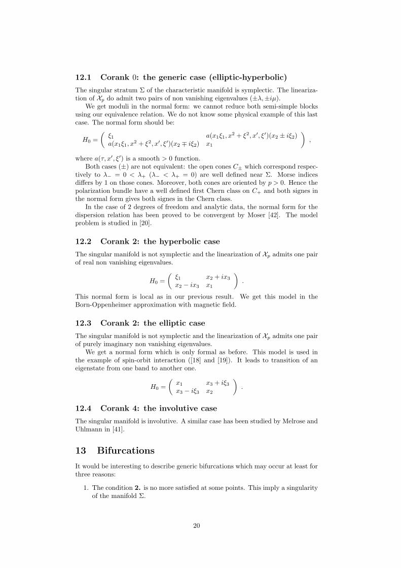
12.1 Corank 0: the generic case (elliptic-hyperbolic)

The singular stratum Σ of the characteristic manifold is symplectic. The lineariza-tion of Xp do admit two pairs of non vanishing eigenvalues (±λ,±iµ).

We get moduli in the normal form: we cannot reduce both semi-simple blocksusing our equivalence relation. We do not know some physical example of this lastcase. The normal form should be:

H0 =

(ξ1 a(x1ξ1, x

2 + ξ2, x′, ξ′)(x2 ± iξ2)a(x1ξ1, x

2 + ξ2, x′, ξ′)(x2 ∓ iξ2) x1

),

where a(τ, x′, ξ′) is a smooth > 0 function.Both cases (±) are not equivalent: the open cones C± which correspond respec-

tively to λ− = 0 < λ+ (λ− < λ+ = 0) are well defined near Σ. Morse indicesdiffers by 1 on those cones. Moreover, both cones are oriented by p > 0. Hence thepolarization bundle have a well defined first Chern class on C+ and both signes inthe normal form gives both signes in the Chern class.

In the case of 2 degrees of freedom and analytic data, the normal form for thedispersion relation has been proved to be convergent by Moser [42]. The modelproblem is studied in [20].

12.2 Corank 2: the hyperbolic case

The singular manifold is not symplectic and the linearization of Xp admits one pairof real non vanishing eigenvalues.

H0 =

(ξ1 x2 + ix3

x2 − ix3 x1

).

This normal form is local as in our previous result. We get this model in theBorn-Oppenheimer approximation with magnetic field.

12.3 Corank 2: the elliptic case

The singular manifold is not symplectic and the linearization of Xp admits one pairof purely imaginary non vanishing eigenvalues.

We get a normal form which is only formal as before. This model is used inthe example of spin-orbit interaction ([18] and [19]). It leads to transition of aneigenstate from one band to another one.

H0 =

(x1 x3 + iξ3x3 − iξ3 x2

).

12.4 Corank 4: the involutive case

The singular manifold is involutive. A similar case has been studied by Melrose andUhlmann in [41].

13 Bifurcations

It would be interesting to describe generic bifurcations which may occur at least forthree reasons:

1. The condition 2. is no more satisfied at some points. This imply a singularityof the manifold Σ.

20

2. There is a change in the normal form involved. For example in the symmetriccase, how do we pass generically from the hyperbolic to the elliptic case?

3. For a d × d system with d ≥ 3, there exists triply and more degeneratedeigenvalue of the classical Hamiltonian at some points.

14 Appendix: coherent states, symplectic spinors

and Gaussian states

14.1 Definitions

A (semi-classical) coherent state is, roughly speaking, a semi-classical state whosemicrosupport is an isotropic submanifold K of the cotangent space. It is desirableto describe nice families of coherent states for which a so-called symbolic calculus isavailable. Of course, such families should be invariant by Fourier Integral Operators.

There are at least 3 available theories of coherent states which are closely related:

1. (Semi-classical) Fourier Integral Operators with complex phase functions stud-ied by Melin and Sjostrand [40].

2. (Semi-classical) Symplectic Spinors studied by Boutet de Monvel and Guillemin[28] and [6], see also [36].

3. Hagedorn’s Semi-classical Wave Packets [29] or Gaussian states..

The first two theories are better adapted to the context of microlocal analysisbeing invariant by Fourier Integral Operators. We will use the second one in whatfollows: we will first give the definition of the semi-classical symplectic spinorsfollowing closely [28]. Then we will define a subset of it, the so-called Gaussianstates, associated to some jet of order ∞ of positive complex Lagrangian manifoldcontaining K; they are very close to Hagedorn’s semi-classical wave packets. Afterthat, we will define the principal symbols of these objects. All our discussion willbe (micro-)local even if it is not always specified.

Definition 1 • Let K0 be the isotropic submanifold of T ?(Rkx ⊕ Rn−k

y ) definedby

K0 = (x, 0; 0, 0) | x ∈ Rk .

We will say that a(x, Y, h) ∈ C∞(Rkx ⊕ R

n−kY ) is a symbol in Σl(K0) if

a(x, ., h) ∈ S(Rn−k) and, for all semi-norms N of the Schwartz space S(Rn−kY ),

and all ε > 0, we have:N(a) = O(hl+ε) ,

uniformly on compacts in Rkx.

• A classical symbol in Σl(K0) is a symbol which admits an asymptotic expan-

sion a(x, Y, h) ∼ hl(∑∞

j=0 hj/2aj(x, Y )

). We will denote by Σl

class(K0) thisspace.

• A symplectic spinor (resp. classical symplectic spinor) uh(x, y) of order lassociated with the isotropic manifold K0 = (x, 0; 0, 0) ⊂ T ?(Rk

x ⊕ Rn−ky ) is

defined by:

uh(x, y) = h−(n−k)/2a(x,y√h, h) ,

where a ∈ Σl(K0) (resp. a ∈ Σlclass(K0)). We will denote a ∈ SSl(K0) (resp.

a ∈ SSlclass(K0)).

21

• If K is an isotropic submanifold of T ?Rn and χ a canonical transformationsuch that χ(K0) = K, we choose an elliptic FIO of order 0 say A and defineSSl(K) = A(SSl(K0)) (resp. SSl

class(K) = A(SSlclass(K0))).

Remark 2 :if K is a Lagrangian submanifold, symplectic spinors associated withK are exactly the Lagrnagian states (WKB-Maslov states).

The proof of the coherence of the previous definition is an easy adaptation ofGuillemin’s argument in [28] (see also [6]). It is clear that, if uh ∈ SSl(K), we haveWFh(uh) ⊂ K.

An example which is useful in our paper is a(x, Y, h) = a0(x, Y )eiP (Y ) log h (seeformula (22)) where a0 is in the Schwartz class w.r. to Y and P is a real valuedpolynomial.

Definition 2 A positive formal Lagrangian manifold along K is a jet of infiniteorder of complex Lagrangian manifold along K whose linear part is a positive La-grangian subspace of ((TK)o/TK)⊗ C.

If K = K0, Λ = Λϕ is defined by a formal series ϕ(x, y) =∑∞

j=2 ϕj(x, y) whereϕj(x, y) is homogeneous of degree j w.r. to y and =ϕ2(x, .) is a strictly positivequadratic form.

Definition 3 A Gaussian state of order l associated to (K0,Λϕ) is defined by

uh(x, y) = ah(x, y)eiϕ(x,y)/h

where a is a classical symbol of order l − (n− k)/2.We will denote by GSl(K0,Λϕ) the corresponding space.We can define GSl(K,Λ) using Fourier integral operators.

Proposition 3 A Gaussian state is a symplectic spinor. If u ∈ GS0(K0,Λϕ), itstotal symbol is

∑∞j=0 Aj(x, Y )hj/2eiϕ2(x,Y ) where Aj(x, Y ) is a polynomial in Y of

degree less than 3j and conversely.

Remark: the “3j” can already be seen in the formula (3.2) in [16].

14.2 Principal symbols

14.2.1 Symplectic spinors

We will now define the principal symbol of a symplectic spinor following [28].Let K be a k−dimensional isotropic submanifold of T ?Rn. We will assume

as in [28] that K is equipped with a metalinear structure. The vector bundleE = TKo/TK of dimension 2(n− k) over K is symplectic. We will assume that itis equipped with a metaplectic structure. It implies that each Lagrangian subbundleis equipped with a metalinear structure. We assume also that Rn is equipped withthe standard metalinear structure.

We want to define the principal symbol of a semi-classical symplectic spinorwhich is a half form: uh(x, y)

√dxdy. We start with a direct sum decomposition

E = L ⊕ L′ of E into a sum of 2 transversal Lagrangian subbundles. The symbolσ(uh) of uh will be an element [ah(x, Y )]

√dxdY where x ∈ K, Y ∈ L and the

equivalent class [.] is in Σ0(L)/Σ12 (L). We use a local trivialisation of L in order to

get functions of (x, Y ). If K = K0, u = h−(n−k)/2ah(x, y/√h)√dxdy, L = 0⊕Rn−k

and L′ = 0 ⊕ (Rn−k)?, we have σ(uh) = [a(x, Y )]√dxdY .

It is now enough to say what is the transformation rule for the symbol underthe action of an elliptic Fourier Integral Operator of order 0: the canonical trans-formation χ such that χ(K0) = K transforms the K0-bundles L0 ⊕ L′

0 ⊂ E0 intothe K-bundles L⊕L′ ⊂ E. It acts in a natural way on principal symbols using the

22

metaplectic representation associated to the linear part of χ. The symbol of A(uh)using this natural action is just obtained by multiplication by the principal symbolof the Fourier Integral Operator.

It remains to speak about the transport equation: we assume that P is a pseudo-differential operator whose principal symbol p vanishes on K and such that Xp istangent to K. If uh ∈ Σ0(K), Puh ∈ Σ1(K) and its principal symbol is given bythe familiar formula

σ(Pu) =1

iLXp

σ(u) + sub(P )σ(u)

where one need to interpret properly as in [28] the Lie derivative!In the matrix case, we need a natural extension of the calculus of [17]. For the

standard examples (Born-Oppenheimer or adiabatic cases), it is enough to considerthe canonical connexion on the polarization bundle.

14.2.2 Gaussian states

The case of Gaussian states is easier to describe: the principal symbol is just ahalf form on the bundle of Lagrangian spaces J1(Λ) over K. If K = K0 andΛ = Λϕ. J1(Λ) = (x, 0; y, ∂ϕ2(x, y)/∂y) and, if we denote by π : J1(Λ) →TK0

Rn the canonical projection, the principal symbol of ah(x, y)eiϕ(x,y)/h√dx ∧ dy

is π?(a0(x, 0)√dx ∧ dy).

References

[1] M. Abramowitz and I. Stegun, Handbook of mathematical functions withformulas, graphs, and mathematical tables. Dover Publication Inc., N.Y.,(1970 ).

[2] V. Arnold, Singularities of Caustics and Wave Fronts. Kluwer (1990).

[3] V. Arnold, On the interior scattering of waves, defined by hyperbolic variationalprinciples. J. Geom. Phys., 5:305-315 (1988).

[4] J.E. Avron and A. Gordon, Born-Oppenheimer wave function near level cross-ing. Phys. Rev. A, 62-06254, 2000.

[5] M. Born und R. Oppenheimer, Zur Quantentheorie der Molekeln. Annal.Phys., 84:457-484, 1927.

[6] L. Boutet de Monvel and V. Guillemin, The Spectral Theory of Toeplitz Op-erators. Princeton Univ. Press (1981).

[7] P. Braam and H. Duistermaat, Normal forms of real symmetric systems withmultiplicity. Indag. Math., N.S., 4(4):407-421, 1993.

[8] Y. Colin de Verdiere, Singular Lagrangian manifolds and semi-classical anal-ysis. Prepublication Institut Fourier no 534 (2001), Duke Math. Journal (toappear).

[9] Y. Colin de Verdiere, Spectres de Graphes. Soc. Math. Fr., 1998.

[10] Y. Colin de Verdiere, The level crossing problem in semi-classical analysis II.The Hermitian case. In preparation, 2002.

[11] Y. Colin de Verdiere, M. Lombardi and J. Pollet, The microlocal Landau-Zenerformula. Annales de l’IHP (Physique theorique), 71:95-127, 1999.

23

[12] Y. Colin de Verdiere et B. Parisse, Equilibre instable en regime semi-classique :I-Concentration microlocale. Commun. in PDE, 19:1535-1563, 1994.

[13] Y. Colin de Verdiere et J. Vey, Le lemme de Morse isochore. Topology, 18:283-293, 1979.

[14] J.-M. Combes, On the Born-Oppenheimer approximation, International Sym-posium on Mathematical Problems in Theoretical Physics (Kyoto Univ., Ky-oto), Lecture Notes in Phys., 39:467–471, 1975.

[15] J.-M. Combes and R. Seiler, Spectral properties of atomic and molecularsystems, Quantum dynamics of molecules (Proc. NATO Adv. Study Inst., Univ.Cambridge), 435–482, 1979.

[16] M. Combescure and D. Robert, Semiclassical spreading of quantum wave pack-ets and applications near unstable fixed points of the classical flow. AsymptoticAnalysis, 14:377-404, 1997.

[17] C. Emmrich and A. Weinstein, Geometry of the transport Equation in Multi-component WKB Approximations. Commun. Math. Phys., 176:701-711, 1996.

[18] F. Faure and B. Zhilinskii, Topological Chern Indices in Molecular Spectra.Phys. Rev. Letters, 85:960-963, 2000.

[19] F. Faure and B. Zhilinskii, Topological properties of the Born-Oppenheimerapproximation and implications for the exact spectrum. Lett. Math. Phys.,55:219-239, 2001.

[20] C. Fermanian-Kammerer, A non-commutative Landau-Zener formula.Prepublication Universite de Cergy-Pontoise, 01/02:1-34, 2002.

[21] C. Fermanian-Kammerer, Une formule de Landau-Zener pour un croisementde codimension 2. Seminaire Equations aux derivees partielles, Ecole Polytech-nique. Expose XXI, 9/04/2002.

[22] C. Fermanian-Kammerer and C. Lasser, Wigner measures and codimensiontwo crossings. preprint mp-arc, 02-186, 2002.

[23] W. Flynn and R. Littlejohn, Normal forms for linear mode conversion andLandau-Zener transitions in one dimension. Ann. Physics, 234(2):334-403,1994.

[24] W. Flynn and R. Littlejohn, Semi-classical theory of spin-orbit coupling, Phys.Rev. A, 45:7697-7717, 1992.

[25] G. Folland, Harmonic Analysis on Phase Space. Princeton Univ. Press, (1989).

[26] P. Gerard et C. Fermanian-Kammerer, Mesures semi-classiques et croisementde modes. Bull. Soc. Math. Fr., 130:123-168, 2002.

[27] P. Gerard et C. Fermanian-Kammerer, A Landau-Zener formula for non-degenerated involutive codimension 3 crossings, Preprint, sept. 2002.

[28] V. Guillemin, Symplectic spinors and PDE, Geometrie Symplectique etPhysique mathematique. Coll. CNRS Aix-en-Provence (1974).

[29] G. Hagedorn, Molecular Propagation through Electron Energy Level Crossings.Memoirs of the AMS, 536 (1994).

24

[30] G. Hagedorn, Higher Order Corrections to the Time-Dependent Born-Oppenheimer Approximation I: Smooth Potentials. Ann. Math., 124:571-590,1986.

[31] G. Hagedorn and A. Joye, Landau-Zener Transitions through small ElectronicEigenvalues Gaps in the Born-Oppenheimer Approximation. Annales de l’IHP(Physique theorique), 68:85–134, 1998.

[32] G. Hagedorn and A. Joye, Molecular Propapagation through small avoidedCrossings of Electron Energy Levels. Rev. Math. Phys., 11:41–101, 1999.

[33] R. Halberg, Localized coupling between surface- and bottom-intensified flowover topography. J. Phys. Oceanogr., 27:977-999, 1997.

[34] P. Holm, Generic elastic Media. Physica Scripta, 44:122-127, 1992.

[35] N. Kaidi et M. Rouleux, Forme normale d’un hamiltonien a deux niveaux presd’un point de branchement (limite semi-classique). C. R. Acad. Sci. Paris,Ser. I, 317(4):359-364, 1993.

[36] M. Karasev and Y. Vorobjev, Integral representations over isotropic subman-ifolds and equations of zero curvature. Adv. Math., 135:220-286, 1998.

[37] M. Klein, A. Martinez, R. Seiler and X. Wang, On the Born OppenheimerApproximation of Wave Operators in Molecular Scattering Theory. Commun.Math. Phys., 143:607-639, 1992.

[38] M. Kline and I. Kay, Electromagnetic theory and geometrical optics. Inter-science publishers, 1965.

[39] L. Landau, Collected papers of L. Landau. Pergamon Press (1965).

[40] A. Melin and J. Sjostrand, Fourier Integral Operators with complex valuedphase functions. Lecture Notes in Math no 459 (1975).

[41] R. Melrose and G. Uhlmann, Microlocal structure of involutive conical refrac-tion. Duke Math. J., 46:571-582, 1979.

[42] J. Moser, On the generalization of a theorem of Liapounoff. Comm. Pure Appl.Math., 11:257-271, 1958.

[43] E. Nelson, Topics in dynamics, I: Flows. Princeton Univ. Press (1969).

[44] P. Pettersson, WKB expansions for systems of Schrodinger operators withcrossing eigenvalues. Asymptotic Anal., 14:1-48, 1997.

[45] J. Vanneste, Mode Conversion for Rossby Waves over Topography. J. Phys.Oceanogr., 31:1922-1925, 2001.

[46] J. von Neumann und E. Wigner, Uber das Verhalten von Eigenwerten beiadiabatischen Prozessen. Phys. Zeit., 30:467-470, 1929.

[47] A. Weinstein, Symplectic manifolds and their Lagrangian submanifolds. Adv.Math., 6:329–346, 1971.

[48] C. Zener, Non-adiabatic crossing of energy levels. Proc. Roy. Soc. Lond. ,137:696–702, 1932.

25