The Kriso Container Ship (KCS) Test Case: an Open Source Overview

VI International Conference on Computational Methods in Marine Engineering MARINE 2015

F. Salvatore, R. Broglia and R. Muscari (Eds)

THE KRISO CONTAINER SHIP (KCS) TEST CASE: AN OPEN SOURCE OVERVIEW

STEFANO GAGGERO*, DIEGO VILLA* AND MICHELE VIVIANI*

* Department of Electric, Electronic, Telecommunication Engineering and Naval Architecture, University of Genoa

Via Montallegro, 1, 16145 Genoa, Italy Web page: http://www.unige.it

Key words: CFD, OpenFOAM, Propellers, KCS, Self-Propulsion

Abstract. In this work, the analysis of the Kriso Container Ship (KCS) test case using the OpenFOAM RANS solver is proposed. Both ship resistance in calm water, propeller open water performances, self-propulsion calculations are proposed and the numerical results are validated by a comparison with the model scale experiments shared in literature and through workshops. The analyses are carried out applying the open source tools, from pre- to post- processing, available in the OpenFOAM environment, namely snappyHexMesh for the generation of the computational mesh, simpleFoam, pimpleDyMFoam, LTSInterFoam for the solution of the various hydrodynamic problems and Paraview for the post-processing of the results. The comparison with the experimental measurements, finally, demonstrates the maturity of these solvers for a reliable and, from an engineering point of view, accurate prediction of some of the peculiar characteristics of the flow ships and propellers are subjected to. 1 INTRODUCTION

In the last years, Computational Fluid Dynamics methods had an exponential growth of application: the increase of the computational performances and the generalization of the Navier-Stokes equation to more complex physical problems made possible the solution of multiple phases and free surfaces flows. Among the fluid dynamics problems the naval architecture community has to deal with, the physical complexity of free surface flows poses some issues on the possibility of numerically predicting the global hydrodynamic parameters (hull resistance, self-propulsion point) of ship hulls and on the confidence that can be expected on the numerical results. Recently, results from literature and from dedicated numerical workshops showed that RANS codes are enough mature for their reliable application on the light of the development of a “Virtual Towing Tank” numerical approach to, at least, complement the usual experimental measurements.

Commercial software proved to be suited for this kind of application: both in the case of propellers and in the case of hulls, results are satisfactory and the ease of use of the code strongly encourages their wide application that is only limited by hardware and license issues. Results from RANS calculations were satisfactory and well in agreement with experiments [1][2] in the case of propeller geometry optimization and, for instance, for very specific problems like tip cavitating vortex inception, both for conventional [22][23] and unconventional tip loaded [3] and ducted [4] configurations. Also for what regards the hydrodynamic features of hulls, RANS

735

Stefano Gaggero, Diego Villa and Michele Viviani

2

and, more in general, viscous approaches reached a well-established maturity that allow their systematic employment for the analysis of a wide range of problems, from hull resistance (see, for instance, the recent Gothenburg 2010 Workshop on CFD in Ship Hydrodynamics) to self-propulsion [5][6][9], added resistance [24] and maneuverability [7][8][11][26][27], using a mix of coupled BEM-RANS approaches and fully viscous computations with free surface effect.

On the other hand, the interest in Open Source approaches, also for the solution of engineering problems, has rapidly grown and their application to marine problems may represent a substantial and convincing alternative [10][12] to commercial software. Especially during the preliminary design phase, as a matter fact, the possibility to accurately and efficiently (both from the numerical and from the economical point of view, being open source codes free from license costs) investigate a rather wide set of alternatives represents a precious added value. Thus, an extensive verification and validation of the Open Source solver is required.

In this work, therefore, the well-known Kriso Container Ship (KCS) [13][14] test case is analyzed only by means, from pre- to post-processing, of Open Source tools, namely the OpenFOAM RANS solver [15]. The KCS ship, thanks to the availability of a wide set of measurements, represents, in fact, a valuable test case that covers many hydrodynamic aspects of hull flows, including self-propulsion conditions. Numerical analyses are carried out to replicate the measurements campaign, including usual hull drag calculation (section 4.1, using the quasi-steady LTSInterFoam solver), propeller open water prediction (section 4.2, using the steady simpleFoam solver with the Multiple Reference Frame feature) and self-propulsion condition (section 4.3, using the moving-mesh, unsteady pimpleDyMFoam solver). The best procedures, starting from mesh generation (with snappyHexMesh) up to solution strategies and post-processing [17], will be highlighted to demonstrate that the OpenFOAM package is a reliable approach even in the maritime field.

2 THE KCS TEST CASE The main characteristics of the reference KCS ship model and its body plan are given in

Table 1 and in Figure 1, respectively. The ship is a 3600 TEU container ship designed at KRISO and tested

at Ship Research Institute (SRI) to provide validation data for the International Workshop on CFD in Ship Hydrodynamic, Gothenburg 2000 and Gothenburg 2010. The model ship has a scale ratio of 1/31.5994 and the Froude Number adopted for the computation is equal to 0.23 that corresponds, in model scale, to an advance speed of 2.196 m/s.

Figure 1: MOERI KCS body plan and KP505 propeller.

736

Stefano Gaggero, Diego Villa and Michele Viviani

3

Table 1: MOERI KCS bare hull characteristics (model scale).

KCS Hull Characteristic KP 505 propeller Characteristics LPP 7.2786 m D 0.25 m LWL 7.3568 m DH/D 0.18 m B 1.0190 m P/D0.7R 0.9967 m D 0.5696 m AE/AO 0.8000 m T 0.3418 m Z 5 Scale ratio 31.5994 CB 0.6508 CP 0.6608

The propeller is the KRISO KP505, a five blade right-handed propeller, whose principal

characteristics, in model scale, are themselves specified in Table 1 and Figure 1. Standard NACA thickness and camber lines are adopted for this propeller having a maximum skew at tip of about 24°.

3 NUMERICAL APPROACH: THE OPENFOAM PACKAGE

3.1 The OpenFOAM solvers OpenFOAM is a collection of libraries devoted to the solution of partial differential

equations, including those belonging to the computational fluid dynamics field and, thanks to its Open Source license, may represent a valid alternative to dedicated commercial softwares. The flow generated around propellers, hulls and appendages can be, from an engineering point of view, successfully approximated by the Reynolds averaging approach of Navier-Stokes equations. Continuity and momentum equations, consequently, can be written, for an incompressible Newtonian fluid, as:

{∇ ∙ �̅�𝐮 = 0

ρ ∂�̅�𝐮∂t + ρ(�̅�𝐮 ∙ ∇�̅�𝐮) = ρ𝐠𝐠 − ∇p̅ + μ∇2�̅�𝐮 + ∇ ∙ 𝐓𝐓𝑅𝑅

(1)

in which �̅�𝐮 and �̅�𝐩 represent, respectively, the average velocity and pressure fields, ρ is the fluid density, μ its dynamic viscosity and 𝐓𝐓𝑅𝑅 is the Reynolds stresses tensor, that in present calculations has been modelled through the two equations 𝑘𝑘 − 𝜔𝜔 𝑆𝑆𝑆𝑆𝑆𝑆 turbulence closure model. The numerical solution of equations (1) is achieved by a cell-centered finite volume method. Depending on the type of problem under investigation (open water propeller, hull resistance and self-propulsion condition) different discretizations schemes for convenctive and diffusive terms were adopted, as well for the time discretization and the coupling between velocities and pressure. Among the standard solvers available within the OpenFOAM library, simpleFoam, LTSInterFoam and pimpleDyMFoam have been selected to address the calculations proposed for the KCS test case.

The simpleFoam solver is a steady and incompressible flow solver based on the segregated approach (each equation can be more efficiently solved separately) which uses the SIMPLE algorithm to overcome the pressure-velocity link problem. Each unknown variable can be evaluated, as a matter of fact, by its reference equation (for instance the x- component of the velocity by the momentum equation along the x- direction) while the pressure can be obtained

737

Stefano Gaggero, Diego Villa and Michele Viviani

4

from the continuity equation. The SIMPLE approach (Semi-Implicit Method for Pressure Linked Equations) by [19], from which the simpleFoam solver, effectively allows to rearrange the discrete form of the continuity equation in order to include, in addition to the velocities, also the pressure, not explicitly present in the equation due to the incompressible nature of the flow, and to iteratively solve the coupling between the two. In the case of open water propeller performances computations, the simpleFoam solver can be applied only if the RANS equations are written in a non-inertial reference frame fixed with the rotating propeller, in which the flow can be considered steady. Between the two possible formulations for rotating reference systems (one in terms of relative velocities, the other in terms of absolute velocities), the well-know Multiple Reference Frame formulation (absolute velocities formulation) is preferred:

{ ∇ ∙ �̅�𝐮𝑎𝑎 = 0ρ(�̅�𝐮𝑟𝑟 ∙ ∇�̅�𝐮𝑎𝑎) = ρ𝐠𝐠 − ∇p̅ + μ∇2�̅�𝐮𝑎𝑎 + ∇ ∙ 𝐓𝐓𝑅𝑅 − ρ(𝝎𝝎 × �̅�𝐮𝑎𝑎) (2)

in which the subscript a represents the velocity in the inertial reference frame, the subscript

r represents the velocity on the rotational reference frame and the relationship between �̅�𝐮𝑎𝑎 and �̅�𝐮𝑟𝑟 is given by �̅�𝐮𝑟𝑟 = �̅�𝐮𝑎𝑎 + 𝝎𝝎 × 𝒓𝒓. The two systems of equations, (1) and (2), are formally very similar, except for the inclusion of the Coriolis term that acts as a momentum source. Therefore, both problems can be addressed with the same solver, with an increase in stability and convergence with respect to the relative velocities formulation (the single reference frame SRFSimpleFoam solver, for instance) due to the reduction of the non-linear terms far from the rotational axis.

PimpleDyMFoam, on the other hand, is a transient flow solver with dynamic/moving mesh capabilities, devoted to the solution of unsteady problems, like the prediction of the influence of a rotating propeller behind the hull (i.e. the self-propulsion condition). Equations (1) are solved using the Pressure Implicit with Splitting of Operator (PISO) algorithm, firstly proposed by [20] or by a hybrid PISO – SIMPLE method (PIMPLE), specifically developed by the OpenFOAM community. The original PISO formulation, as a matter of fact, suffers of excessive sensitiveness from the initial conditions and reduced stability with respect to SIMPLE approaches. PIMPLE, on its turn, is a step towards the accuracy of PISO-based algorithm with the stability typical of SIMPLE approaches. The dynamic capabilities of the solver, moreover, allows mesh deformations and mesh motion (achieved by sliding interfaces) that is mandatory for the inclusion of the rotating propeller behind the hull. Arbitrary Mesh Interfaces [18] permit the exchange of informations and the conservation of fluxes between non-conformal adjacent patches by a weighted interpolation between the portions of “master” and “slave” surfaces.

The presence of the free surface poses further problems for the solution of equations (1). Among the techniques developed to account for two-phase flows (mainly interface-tracking and interface-capturing), the interface capturing approach based of the volume of fluid (VOF) is one of the more commonly used for the solution of complex free-surface flows between immiscible and non-reactive flows. Interface-tracking methods, as a matter of fact, even being able to capture very sharply the interface between flow phases, suffer of excessive computational time due to the continuous deformation of the computational mesh required to track the interface itself, and generally fail when the free surface folds onto itself as when wave breaking and sprays occur. Volume of fluid approaches, instead, solve the free surface as the solution of the advection of a scalar function α (ranging from 0 to 1) denoting the volume

738

Stefano Gaggero, Diego Villa and Michele Viviani

5

fraction of the fluid on each cell. Using the volume fraction itself to determine the proprieties of the fluid mixture (that obey to RANS equations (1)) as a weighted mean:

ρ = ρwater ∙ α + ρair ∙ (1 − α)μ = μwater ∙ α + μair ∙ (1 − α) (3)

the partial differential equation that governs the evolution of the scalar function α can be written as:

∂α∂t + ∇ ∙ (α�̅�𝐮) = 0 (4)

The discontinuity of the function α at the interface, represented by the jump, from 1 to 0, of

the scalar quantity itself, commonly requires some special treatment in order to limit the numerical smearing and to predict the sharpest possible free surface shape.

OpenFOAM uses a modified version [16] of equation (4), based on the compression of the interface with an artificial velocity 𝐮𝐮𝑟𝑟 (scaled by a user defined factor) that “pushes” the volume fraction toward the free surface. The α(1 −α) term ensures that the compression takes place only in proximity of the interface:

∂α∂t + ∇ ∙ (α�̅�𝐮) + ∇ ∙ (α(1 − α)𝐮𝐮𝑟𝑟) = 0 (5)

Another feature implemented in the OpenFOAM libraries lets also to adopt a custom quasi-

steady approach (the LTSInterFoam library) to solve for the time evolution of the free surface. Quasi-steady approaches are useful each time the attention is only to the steady-state solution reached at the end of a non influent transient computation and, for this reason, the complex physic that regulates the phenomenon and all the transient behaviour of the solution can be partially neglected (violating, consequently, the underlying equations of conservation) in order to reach as fast as possible the stable steady-state condition. The LTSInterFoam solver is based on the Local Time Stepping approach (a bounded, first order accurate, implicit scheme), in which the time step is manipulated for each individual cell in the mesh, making it as high as possible according to the local Courant number to force the simulation to quickly reach steady-state. A smoothing of the unphysical variation of the time steps across the whole domain cells is applied to prevent the instabilities caused by the sudden changes in the time scale.

3.2 The snappyHexMesh tool The generation of accurate discretization meshes represents a crucial aspect for the reliable

prediction of the flow features around ships and propellers. OpenFOAM provides the mesh generation utility snappyHexMesh that has been adopted to setup all the calculation grids used in present calculations. SnappyHexMesh is a Cartesian hexa-dominant mesh generation utility that can handle quite accurately complex geometries (starting from standard stereo lithographic representation of the geometry surfaces) with the capability of prism layers generation, feature curves and local refinements handling. The snappyHexMesh utility generates 3-dimensional meshes containing hexahedra and split-hexahedra that approximately conforms to the surface

739

Stefano Gaggero, Diego Villa and Michele Viviani

6

by iteratively refining a starting mesh and morphing the resulting split-hex mesh to the surface. The discretization mesh is obtained as the result of three steps: castellation, snapping and prism layer insertion. Starting from a purely Cartesian mesh, first the cells that do not belong to the computation domain (i.e. those inside the hull, for instance) are removed. As a second step the cells close to the geometry surfaces are “snapped”, projecting their vertices, to the surfaces themselves and the entire mesh is smoothed accordingly to a set of user defined mesh quality parameters. Finally the prism layers are inserted by projecting back the mesh from the surfaces by a specified thickness in the direction normal to the surface itself and inserting prismatic layers if a set of quality criteria are satisfied. An example of the resulting mesh after snappying and adding prism layers, in the case of the KP505 propeller, is reported in Figure 2.

Figure 2: Snapped and Prism Layer addition steps at the KP505 blade leading edge. The snappyHexMesh tool, however, is not free of issues, even in the case of rather simple

geometries like the almost planar and developable surfaces. In particular, close to the feature curves, where sharp edges have to be followed by the mesh, and in correspondence to the transition between patches having different prism layers characteristics (i.e. the hull, with prisms, and the symmetry plane, without) the prism layer addition step could fail (even with an accurate choice of the snapping parameters). This may introduce some non-negligible deformations of the mesh, whose consequences on the accuracy of the hydrodynamic solution can be serious. In particular, in correspondence to the symmetry plane or to the periodic interfaces, the prism layer may not be properly extruded because the initial snapped cells are not slipped correctly. In addition, the sharp edges (the blade trailing edge, for instance, the transom of the hull) may introduce some deformations and errors for the addition of the prism layers, whose influence on the hydrodynamic flow features has to be verified each time.

4 RESULTS

Numerical calculations have been carried out for the KCS hull at the design speed in order to validate numerical calculations in terms of hull resistance, wave field and hull wake on the propeller plane. The open water KP505 propeller performances were taken into account to verify the accuracy of the numerical calculation in the case of rotating/periodic domain computations. Self-propulsion prediction have been considered to assess the mutual interaction between the hull and the propeller and the reliability of moving mesh with sliding interfaces in the relatively complex case of unsteady flow. Calculation meshes, obtained with the open

740

Stefano Gaggero, Diego Villa and Michele Viviani

7

source tool snappyHexMesh, have been arranged, on the light of previous experience [12][25], to have affordable calculations times without excessive worsening in computation accuracy.

4.1 Bare Hull Resistance Calculations of the KCS hull have been carried out at the design speed using the

LTSInterFoam solver. A bounded second order accurate scheme is adopted for the discretization of all the spatial derivatives. Gradients are computed using second order Gaussian integration, while laplacian terms are treated with a conservative, unbounded second order approach. Convection of turbulent quantities is approximated with first order schemes. The PIMPLE algorithm was selected to couple the velocities and the pressure fields. The second order accurate vanLeer scheme is used to solve the convective terms of the VOF equation. The discretization mesh consists in a total of 1.3 Million cells arranged, as shown in Figure 3, in order to have anisotropic refinements (along the vertical direction) in correspondence to the free surface and sufficient spatial resolution at the hull bow and at the stern to reliably predict the bow wave and the hull wake.

Figure 3: Details of the computational mesh at bow and in correspondence of the anysotropic refinement on the free surface.

A summary of the results is shown in Figure 4 to Figure 7. Hull generated wave field is

compared with the experiments; more in detail, two wave cuts, at y/Lpp = 0.0741 and 0.1509, are considered to appreciate the accuracy of the numerical calculations. Predicted total hull resistance is only slightly underestimated. With respect to an experimental value of the total resistance coefficient of 3.5210-3, the computed value of 3.4510-3 is only 2% underpredicted, showing an satisfactory accuracy of the numerical approach especially on the light of a relatively coarse mesh arrangement specifically selected to keep computational times daily affordable. In addition, the convergence of the solution, achieved after only 7000 iterations, is fast and usually better respect to a fully unsteady treatment of the volume of fluid equations, commonly used to solve the multi-phase problems [6].

The overall quality of the solution can be better appreciated by the comparison of the wave cuts of Figure 5. The predicted wave field is in very good agreement with the measurements.

741

Stefano Gaggero, Diego Villa and Michele Viviani

8

Figure 4: Comparison between measured and computed wave field. Top: LTSInterFoam numerical calculations. Bottom: experimental measurements.

At bow, in particular, the agreement is excellent in terms of both wave elevation and shape of the divergent wave groups. At stern the computed wave height is slightly overestimated but the position of the humps and troughs of the longitudinal and transversal waves is well predicted. Only at stern, relatively far from the hull where the discretization of the domain and of the free surface is coarse, the computed wave is smeared and the peaks slightly shifted with respect to the measurements.

Figure 5: Comparison between measured and computed longitudinal wave cuts: y/Lpp = 0.0741 (left)

and y/Lpp = 0.1509 (right).

The analysis of the predicted nominal wake on the propeller plane of Figure 7 confirms the reliability of the numerical computations. With respect to measurements, the predicted wake is only slightly less “flat” and thicker under the stern, which is more evident in correspondence of the symmetry plane.

-0.006

-0.004

-0.002

0.000

0.002

0.004

0.006

-1.50 -1.00 -0.50 0.00 0.50 1.00 1.50 2.00

z/L

pp

x/Lpp

Experimental LTSInterFOAM

-0.006

-0.004

-0.002

0.000

0.002

0.004

0.006

-1.50 -1.00 -0.50 0.00 0.50 1.00 1.50 2.00

z/L

pp

x/Lpp

Experimental LTSInterFOAM

742

Stefano Gaggero, Diego Villa and Michele Viviani

9

Figure 6: Predicted versus measured hull resistance at Fn = 0.23.

Tangential and radial components of the velocity field, in addition, show a reasonable

counter-clockwise rotation and highlight, as from the experiments, the presence of vortices.

Figure 7: Comparison between measured and computed Nominal wave field on the propeller plane. Left: experimental measurements. Right: LTSInterFoam numerical calculations.

4.2 OpenWater Propeller Performances The prediction of open water propeller performances has been carried out with the steady

solver simpleFoam together with a Multiple Reference Frame approach devoted to the solution of Navier-Stokes equation in a rotating reference frame. This approach allows exploiting the axial symmetry of the propeller to solve the flow only in a fraction of the computational domain by using periodic boundary conditions.

0 1000 2000 3000 4000 5000 6000 7000 8000 9000 100000.0000

0.0010

0.0020

0.0030

0.0040

0.0050

0.0060

0.0070

0.0080

0.0090

Iteration

CT

LTSInterFoamExperiments

743

Stefano Gaggero, Diego Villa and Michele Viviani

10

Figure 8: Periodic computational domain and pressure distribution CPN on the KP505 propeller at J = 0.7.

In particular, due to the shape of the propeller under investigation, a computational domain

in the form of a blade passage, as that presented in Figure 8, has been adopted, while periodic boundary conditions have been implemented using the Arbitrary Mesh Interface boundary option, based on the work by [18]. The resulting computation mesh, setup with the snappyHexMesh utility, consists in 1.2 Million cells per blade. Second order, bounded, schemes were adopted to discretize the convective terms. Gradients are computed using second order Gaussian integration, while laplacian terms are treated with a bounded, second order, scheme.

Figure 9: Open Water propeller performances for KP505.

Computed performances are compared with measurements in Figure 9. Even in this case, the

overall agreement between calculations and experiments is satisfactory. For a relatively wide range of advance coefficient predicted performances, both in terms of thrust and torque, differ from the measurements less than 2% and only for higher values of advance coefficient numerical predictions show a rather different slope of the performance curves.

0

0.1

0.2

0.3

0.4

0.5

0.6

0.7

0.8

0 0.1 0.2 0.3 0.4 0.5 0.6 0.7 0.8 0.9 1 1.1J

KT exp.10KQ exp.KT simpleFoam10KQ simpleFoam

744

Stefano Gaggero, Diego Villa and Michele Viviani

11

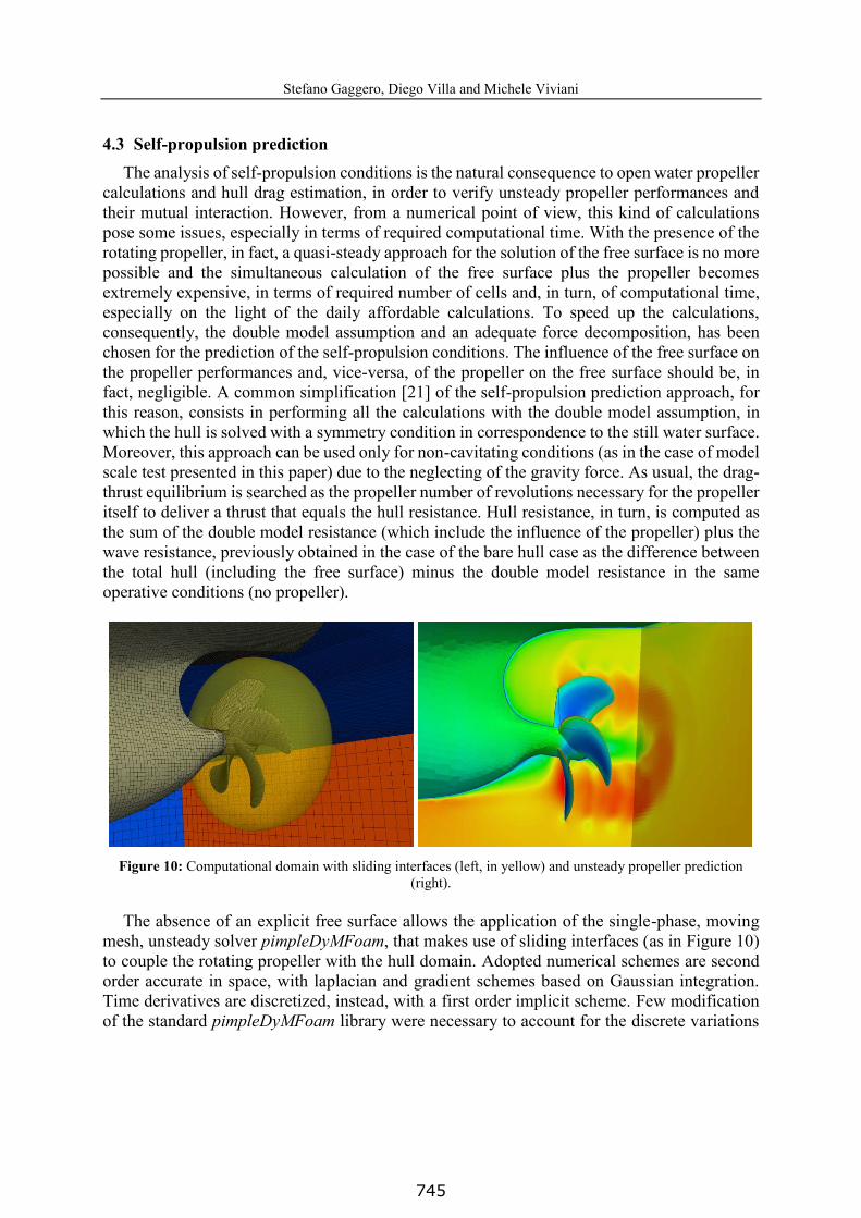
4.3 Self-propulsion prediction The analysis of self-propulsion conditions is the natural consequence to open water propeller

calculations and hull drag estimation, in order to verify unsteady propeller performances and their mutual interaction. However, from a numerical point of view, this kind of calculations pose some issues, especially in terms of required computational time. With the presence of the rotating propeller, in fact, a quasi-steady approach for the solution of the free surface is no more possible and the simultaneous calculation of the free surface plus the propeller becomes extremely expensive, in terms of required number of cells and, in turn, of computational time, especially on the light of the daily affordable calculations. To speed up the calculations, consequently, the double model assumption and an adequate force decomposition, has been chosen for the prediction of the self-propulsion conditions. The influence of the free surface on the propeller performances and, vice-versa, of the propeller on the free surface should be, in fact, negligible. A common simplification [21] of the self-propulsion prediction approach, for this reason, consists in performing all the calculations with the double model assumption, in which the hull is solved with a symmetry condition in correspondence to the still water surface. Moreover, this approach can be used only for non-cavitating conditions (as in the case of model scale test presented in this paper) due to the neglecting of the gravity force. As usual, the drag-thrust equilibrium is searched as the propeller number of revolutions necessary for the propeller itself to deliver a thrust that equals the hull resistance. Hull resistance, in turn, is computed as the sum of the double model resistance (which include the influence of the propeller) plus the wave resistance, previously obtained in the case of the bare hull case as the difference between the total hull (including the free surface) minus the double model resistance in the same operative conditions (no propeller).

Figure 10: Computational domain with sliding interfaces (left, in yellow) and unsteady propeller prediction (right).

The absence of an explicit free surface allows the application of the single-phase, moving

mesh, unsteady solver pimpleDyMFoam, that makes use of sliding interfaces (as in Figure 10) to couple the rotating propeller with the hull domain. Adopted numerical schemes are second order accurate in space, with laplacian and gradient schemes based on Gaussian integration. Time derivatives are discretized, instead, with a first order implicit scheme. Few modification of the standard pimpleDyMFoam library were necessary to account for the discrete variations

745

Stefano Gaggero, Diego Villa and Michele Viviani

12

of the propeller rate of revolution needed to iteratively reach equilibrium between delivered propeller thrust and hull resistance.

Calculations have been carried out with a mesh of about 1.6 Million cells, 600 thousands of which devoted to the discretization of the propeller blades. With respect to open water calculations (in that case 1.2 Million cells per blade were used, leading to at least 6 Million cells for an equivalent discretization) a significant coarsening of the mesh has been accepted to maintain the simulation within tolerable calculations time. The double model assumption, first, allows avoiding the mesh refinement in correspondence to the free surface. On the other hand, the analysis is focused on the influence the propeller has on the hull more than on the accurate prediction of the flow field of the propeller wake, where much of the cells were clustered in open water simulations: a rather coarse mesh for the propeller, consequently, is sufficient to adequately characterize the hull-propeller interaction.

A summary of the results of self-propulsion calculations is reported in Table 2. The overall agreement with experiments is satisfactory but some non-negligible differences have to be highlighted. Even if the prediction of the propeller rate of revolution and of the wake fraction is barely satisfactory on the light of similar calculations with coupled BEM-RANS approaches [6] and full RANS calculations [21], the prediction of the thrust deduction is poor, with differences of 5% with respect to literature results of 2-3% [21].

Table 2: Self-Propulsion calculations.

Unbalance (T-R)/T Prop. rps Prop. KT (1-w) (1-t) R CT self-prop. Step 1 -7.8% 9.00 0.1596 0.7479 0.9127 1.011 0.003697 Step 2 7.5% 9.40 0.1776 0.7483 0.8757 1.028 0.003798 Step 3 0.5% 9.20 0.1694 0.7471 0.8914 1.021 0.003754 (-3.2%) (-1.4%) (-5.0%) (+5.4%) (+1.1%) (-5.3%)

Exp. 9.50 0.1720 0.7860 0.8460 1.011 0.003966

These differences can be attributed to the interaction between various phenomena and to the discrepancies already highlighted in the analysis of the hull and of the propeller. The total hull resistance is slightly underestimated and, in turn, a lower propeller rps can be expected. On the other hand the propeller performances, even if only steady open water calculations are considered, are numerically underpredicted, leading to an overestimation of the propeller rate of revolution and to a overestimation of the wake deduction factor derived, as usual practice, from the (numerical) open water propeller curves. These two errors, which act in an opposite way with respect to the predicted propeller rate of revolution, could not completely justify the discrepancies in terms of thrust deduction that could be, on the contrary, ascribed to the underestimation of the interaction between the hull and the propeller. The coarse mesh that was chosen due to the constraints on computational resources may explain the lower influence the propeller pressure fields has on the hull. With respect to usual calculations of hull or propellers, in fact, the setup of the computational mesh is more problematic because of the sliding interfaces and the multiple regions arrangements. Moreover, if compared with other meshing tools, the coarsening with snappyHexMesh is rather crude near the surfaces and the overall quality of the mesh, in case of relatively coarse meshes, is generally low, with a detrimental influence on the prediction of the flow features at the stern of the ship. The discrepancies

746

Stefano Gaggero, Diego Villa and Michele Viviani

13

highlighted in the self-propulsion analysis are confirmed also by the comparison, presented in Figure 11 of the mean flow on a plane 0.25D downstream the propeller. Because of a propeller delivering a lower thrust, the axial component of the downstream flow is less accelerated with respect to the experimental measurements. On the contrary, the swirl is slightly overestimated.

Figure 11: Measured (left) and predicted (right) mean flow on a plane 0.25D aft the propeller plane.

5 CONCLUSIONS

The successful application of the OpenFOAM RANS libraries for the prediction of the hydrodynamic features of the flow around hulls and propellers has been demonstrated through a methodical comparison of the computed results with the experimental measurements available for the well-knows KCS test case. Regular predictions of calm water resistance and propeller open water characteristics show a very satisfactory agreement with experiments. Errors are about few percent with respect to measurements and the overall convergence of the solution is generally fast thanks to specific quasi-steady solvers. For these problems, prediction of calm water resistance and open water propeller characteristics, the overall quality of the discretization mesh setup through the open source snappyHexMesh utility is adequate, except few issues close to feature lines or related to prism layer extrusion that, however, seems not sufficient to degrade excessively the main features of the flow solution. In the more demanding case of self-propulsion simulations, the accuracy of the numerical prediction is only sufficient. The coarse mesh arrangements and its non-optimal setup due to the limitations of the snappyHexMesh utility can negatively affect the predictions, which are particularly problematic if the thrust deduction factor is considered. However also the non-optimal results from self-propulsion calculations represent a step towards the wide application of open source tools, which main limitation is represented by the mesh generation phase.

747

Stefano Gaggero, Diego Villa and Michele Viviani

14

REFERENCES [1] Gaggero S., Tani, G., Viviani M. and Conti, F., A study on the numerical prediction of

propellers cavitating tip vortex, Ocean Engineering, Volume 92 (2014), pp. 137 – 161, ISSN:0029-8018, DOI:10.1016/ j.oceaneng.2014.09.042.

[2] Bertetta D., Brizzolara S., Gaggero S., Viviani M. and Savio, L., CPP propeller cavitation and noise optimization at different pitches with panel code and validation by cavitation tunnel measurements, Ocean Engineering, Volume 53 (2012), pp. 177 – 195, ISSN:0029-8018, DOI:10.1016/j.oceaneng.2012.06.026.

[3] Bertetta D., Brizzolara S., Canepa E., Gaggero S. and Viviani M., EFD and CFD characterization of a CLT propeller, International Journal of Rotating Machinery, Volume 2012, Article ID 348939, p.1-23, ISSN: 1023-621X (Print), ISSN: 1542-3034 (Online), DOI:10.1155/2012/348939.

[4] Gaggero S., Rizzo C.M., Tani G. and Viviani M., EFD and CFD design and analysis of a propeller in decelerating duct, International Journal of Rotating Machinery, Volume 2012, Article ID 823831, ISSN: 1023-621X (Print), ISSN: 1542-3034 (Online), DOI:10.1155/2012/823831.

[5] Castro, A.M., Carrica, P.M. and Stern, F., Full scale self-propulsion computations using discretized propeller for the KRISO container ship KCS, Computers and Fluids, Volume 51 (2011), pp. 35 – 47.

[6] Gaggero S., Villa, D. and Brizzolara S., Simulation of ship in self-propulsion with different CFD methods: from actuator disk to potential flow coupled solvers to fully unsteady RANS models, Proceedings of the RINA Marine CFD Conference 2011, London, England, March 2011.

[7] Mofidi, A. and Carrica, P.M., Verification of 20/5 zigzag maneuver for a container ship with direct moving rudder and propeller, Workshop on Verification and Validation of Ship Manoeuvering Simulation Methods, SIMMAN 2014, Copenhagen, December 2014.

[8] Sadat-Hosseini, H. and Stern, F., 5415 Maneuvering Simulation Using CFD Free Running and CFD-based SI, Workshop on Verification and Validation of Ship Manoeuvering Simulation Methods, SIMMAN 2014, Copenhagen, Denmark, December 2014.

[9] Wöckner, K., Greve, M., Scharf, M., Abdel-Maksoud, M. and Rung, T., Unsteady Viscous/Inviscid Coupling Approaches for Propeller-Flow Simulations, 2nd International Symposium on Marine Ship Propellers, Hamburg, Germany, June 2011.

[10] Shen, Z., Wan, D. and Carrica, P.M. RANS Simulations of Free Maneuvers with Moving Rudders and Propellers using Overset Grids in OpenFOAM, Workshop on Verification and Validation of Ship Manoeuvering Simulation Methods, SIMMAN 2014, Copenhagen, Denmark, December 2014.

[11] Woolliscroft, M. and Maki, K., Simulations of Static and Dynamic Maneuvering Tests Using a Linearized URANS Method, Workshop on Verification and Validation of Ship Manoeuvering Simulation Methods, SIMMAN 2014, Copenhagen, Denmark, December 2014.

[12] Gaggero, S., Villa, D. and Ferrando, M., An OpenSource Approach for the Prediction of Planning Hull Resistance, 10th Symposium on High Speed Marine Vehicles, HSMV2014, Naples, Italy, October 2014.

748

Stefano Gaggero, Diego Villa and Michele Viviani

15

[13] Van, S.H., Kim, W.J., Yim, G.T., Kim, D.H., and Lee, C.J., Experimental Investigation of the Flow Characteristics Around Practical Hull Forms, Proceedings 3rd Osaka Colloquium on Advanced CFD Applications to Ship Flow and Hull Form Design, Osaka, Japan, 1998.

[14] Kim, W.J., Van, D.H. and Kim, D.H., Measurement of flows around modern commercial ship models, Exp. in Fluids, Vol. 31, pp 567-578, 2001.

[15] OpenFOAM Foundation, OpenFOAM 2.3.0, The OpenFOAM Foundation, OpenCFD Ltd, 2014.

[16] Rusche, H., Computational fluid dynamics of dispersed two-phase flows at high phase fractions. PhD thesis, Imperial College, London, UK, 2002.

[17] Henderson, A., Ahrens, J. and Law, C., The ParaView Guide, Kitware Inc., Clifton Park, NY, USA, 2004.

[18] Farrell, P.E. and Maddison, J.R., Conservative interpolation between volume meshes by local Galerkin projection, Computer Methods in Applied Mechanics and Engineering, vol. 200 (2011) pp. 89 – 100.

[19] Patankar, S. V., Numerical Heat Transfer and Fluid Flow, Taylor & Francis, 1980. [20] Issa, R., Solution of the implicit discretized fluid flow equations by operator-splitting,

Journal of Computational Physics, Vol. 62 (1986). [21] Krasilnikov, V.I., Self-Propulsion RANS Computations with a Single-Screw Container

Ship, Third International Symposium on Marine Propulsors, SMP 2013, Launceston, Tasmania, 2013.

[22] Brizzolara, S., Villa, D. and Gaggero, S., A systematic comparison between RANS and Panel Methods for Propeller Analysis, Proceeding of 8th International Conference on Hydrodynamics ICHD2008, Nantes France, 30 September-3 October 2008, Vol. 1, pp. 289 – 302.

[23] Gaggero, S., Villa, D. and Brizzolara, S., RANS and Panel Methods for Unsteady Flow Propeller Analysis, Journal of Hydrodynamics, Ser. B, Volume 22 (2010), Issue 5, Supplement 1, pp. 564 – 569.

[24] Grasso, A., Villa, D., Brizzolara, S. and Bruzzone, D., Nonlinear motions in head waves with a RANS and a potential code, Journal of Hydrodynamics, Ser. B, Volume 22 (2010), Issue 5, Supplement 1, pp. 172 – 177.

[25] Gaggero S., Viviani M., Villa D., Bertetta D., Vaccaro C. and Brizzolara S., Numerical and Experimental Analysis of a CLT Propeller Cavitation Behavior, Proceedings of the 8th International Symposium on Cavitation, CAV2012, Singapore, August 2012.

[26] Dubbioso, G., Durante, D., Broglia, R., and Di Mascio, A., Maneuvering Prediction of a Twin Screw Vessel with different stern appendages configuration. Proc. of 29th ONR Symposium on Naval Hydrodynamics. Gothenburg, Sweden, August 2012.

[27] Cura-Hochbaum, A. and Uharek, S., Prediction of the Manoeuvring behavior of the KCS based on Virtual Captive Tests, Workshop on Verification and Validation of Ship Manoeuvering Simulation Methods, SIMMAN 2014, Copenhagen, Denmark, December 2014.

749