The kinetic origin of the fluid helicity – a symmetry

in the kinetic phase space

Z. Yoshida1 and P. J. Morrison2

1 Graduate School of Frontier Sciences, University of Tokyo, Kashiwa, Chiba

277-8561, Japan2 Department of Physics and Institute for Fusion Studies, University of Texas at

Austin, TX 78712-1060, USA

Abstract. Helicity, a topological degree that measures the winding and linking of

vortex lines, is preserved by ideal (barotropic) fluid dynamics. In the context of the

Hamiltonian description, the helicity is a Casimir invariant characterizing a foliation of

the associated Poisson manifold. Casimir invariants are special invariants that depend

on the Poisson bracket, not on the particular choice of the Hamiltonian. The total mass

(or particle number) is another Casimir invariant, whose invariance guarantees the

mass (particle) conservation (independent of any specific choice of the Hamiltonian).

In a kinetic description (e.g. that of the Vlasov equation), the helicity is no longer

an invariant (although the total mass remains a Casimir of the Vlasov’s Poisson

algebra). The implication is that some “kinetic effect” can violate the constancy of the

helicity. To elucidate how the helicity constraint emerges or submerges, we examine

the fluid reduction of the Vlasov system; the fluid (macroscopic) system is a “sub-

algebra” of the kinetic (microscopic) Vlasov system. In the Vlasov system, the helicity

can be conserved, if a special helicity symmetry condition holds. To put it another

way, breaking helicity symmetry induces a change in the helicity. We delineate the

geometrical meaning of helicity symmetry, and show that, for a special class of flows

(so-called epi-2 dimensional flows), the helicity symmetry is written as ∂γ = 0 for a

coordinate γ of the configuration space.

arX

iv:2

103.

0399

0v1

[ph

ysic

s.fl

u-dy

n] 6

Mar

202

1

kinetic helicity 2

1. Introduction

Casimir invariants of noncanonical Hamiltonian systems (flows on Poisson manifolds)

are universal invariants independent of any particular choice of the Hamiltonian, and

therefore represent types of topological constraints inherent to Poisson manifold phase

spaces [1]. Every orbit is constrained to Casimir leaves, level-sets of Casimirs, so the

gradient of a Casimir is transverse to the leaf its constancy defines. This means that the

gradient of the Casimir belongs to the kernel of the Poisson matrix (the 2-vector that

maps the gradient of the Hamiltonian to the Hamiltonian vector field). By “degenerate”

we mean that the Poisson matrix defined on the Poisson manifold has a nontrivial kernel.

We note that the element of the kernel (covector) is not necessarily integrable, i.e., the

gradient of some scalar. However, a Casimir is such an integral, yielding a foliation of

the Poisson manifold by its level-sets.

When a Casimir is given, one can interpret it as an adiabatic invariant, made

“variable” by adding an angle variable to complete a conjugate action-angle pair [2].

After embedding the noncanonical Poisson manifold into the inflated phase space, the

constancy of the Casimir can then be re-interpreted as arising from a symmetry with

respect to the supplementary angle variable; hence, its constancy is now attributed to

this specific symmetry of the Hamiltonian. The example of Sec. 2.2 will delineate such a

relation from the opposite viewpoint: starting from the canonical (symplectic) Poisson

manifold sp(6,R), we derive the noncanonical so(3) Lie-Poisson algebra by reduction [3].

Restricting the 6 dimensions of sp(6,R), represented by the position vector q and the

momentum vector p, to 3 dimensions determined by the angular momentum ` = q×p,

the system reduces to the 3-dimensional so(3) Lie-Poisson manifold with the magnitude

|`| becoming the Casimir of the so(3) Lie-Poisson bracket. Consequently, the effective

available phase space shrinks to the 2 dimensional spherical surface |`| = constant.

A physical example of such a reduced angular momentum system is the Euler top,

which is a point mass bound to the origin of the coordinate space by a rigid, mass-

less rod. Then, the angle between the position q and the momentum p is fixed to be

perpendicular. If this angle is allowed to vary (for example, if the rod is not sufficiently

rigid), the constancy of the Casimir |`| is broken (see Sec. 2.2), i.e., “rigidity” is the root

cause of the Casimir. More precisely, for the Casimir to be invariant, there must be a

distinct separation of the time scale (or energy) between the dynamics of the top and

the change of the angle variable. Consequently, from this point of view we may interpret

the Casimir as an adiabatic invariant.

In fluid mechanics, the helicity is a Casimir of the Hamiltonian formalism of the

ideal (barotropic) fluid model [4], which is a measure of the winding and linking of vortex

lines [5]. Interestingly, in a kinetic description (e.g. the Vlasov equation; see Sec. 3), the

helicity is no longer an invariant. This implies that some “kinetic effect” can violate the

topological constraint associated with the helicity. It is known that the ideal fluid system

can be formulated as a reduction (subalgebra) of the Vlasov system [1]. In the Vlasov

system, the helicity can still be conserved, if a special helicity symmetry condition holds.

kinetic helicity 3

To put it another way, braking of the helicity symmetry allows for a changing helicity.

The aim of this work is to elucidate the geometrical meaning of the helicity symmetry,

and study how the topological constraint associated with the helicity invariance can

be broken in kinetic theory. For a special class of flows (so-called epi-2 dimensional

flows [6]), we will show that the helicity symmetry is written as ∂γ = 0 with γ being a

configuration space coordinate.

2. Casimir and gauge symmetry in a “reduced system” – examples

Because Casimirs play a central role in this work, we explain, by simple examples, how

a Casimir is “created” by a reduction of some kind, and how it is related to the gauge

symmetry of the reduction.

2.1. Reduction of canonical variables

We start with the canonical Hamiltonian system of a point mass moving in Rn with the

phase space being M = R2n. The coordinates of a point of M represent a state vector,

z = (q,p)T, with position q and momentum p. On C∞(M), the space of observables,

we define the canonical Poisson bracket

[G,H] =n∑j=1

(∂qjG) (∂pjH)− (∂qjH) (∂pjG). (1)

Denoting by ∂zG ∈ T ∗M the gradient of G ∈ C∞(M), and by 〈x,y〉 the natural pairing

of x ∈ T ∗M and y ∈ TM , we may rewrite (1) as

[G,H] = 〈∂zG, J∂zH〉, (2)

with the Poisson operator (matrix)

J =

(0 I

−I 0

)∈ Hom(T ∗M,TM). (3)

The Hamiltonian vector z ∈ TM is given by

z = J∂zH.

We assume n = 2 and denote the corresponding symplectic manifold by M4 (= R4).

As a trivial example of reduction, we suppose all observables are independent to q2 and

p2. Then, the Poisson bracket evaluates as

[G,H]M2 = (∂q1G) (∂p1H)− (∂q1H) (∂p1G) , (4)

which defines a canonical Poisson algebra on the submanifold M2 = z2 = (q1, p1)T =

R2, which is embedded in M4 as a leaf z ∈ M4; q2 = c, p2 = c′, where c and c′ are

arbitrary constants.

An interesting situation occurs when we only suppress the coordinate q2 in the set

of observables: the reduced phase space is the 3-dimensional submanifold M3 = z3 =

kinetic helicity 4

(q1, p1, p2)T. For G and H satisfying ∂q2G = ∂q2H = 0, the Poisson bracket evaluates

the same as (4) and we may write

[G,H]M3 = 〈∂z3G, J∂z3H〉

with the Poisson operator (matrix)

J =

0 1 0

−1 0 0

0 0 0

,

whose rank is two. Therefore M3 is a degenerate Poisson manifold. The kernel of this

J includes the vector (0, 0, 1)T, which can be integrated to define a Casimir C = p2.

Therefore, the effective dimension is further reduced down to two; the state vector z

can only move on the 2-dimensional leaf M2. Evidently the “freezing” of C = p2 is due

to the suppression of its conjugate variable q2.

When we observe M3 from M4, the reduction (i.e. the suppression of the coordinate

q2 in the observables) means the symmetry ∂q2 = 0. As usual, the the integral of

motion p2 in M4 arises because q2 is ignorable, i.e., if the Hamiltonian has the symmetry

∂q2H = 0.

The variable q2 conjugate to the Casimir C = p2 can be regarded as a gauge

parameter. The gauge group (denoted by AdC), which does not change the submanifold

M3 embedded in M4, is generated by the adjoint action

adC = [, C] = ∂q2 ,

implying that the gauge symmetry is written as ∂q2 = 0. This is evident, because the

state vector z3 = (q1, p1, p2)T ∈M3 is independent of q2.

A similar reduction occurs when we consider the canonical pair,

µ =1

2

[(q2)2 + (p2)2

], θ = tan−1

(q2

p2

).

If we suppress θ in the set of observables, µ becomes the Casimir of M ′3 = M4/θ. The

motion of a magnetized particle is an example, where µ corresponds to the magnetic

moment, and θ to the gyration angle. When the gyro period is negligibly shorter than

the time scale of interest, µ can be dealt with as an adiabatic invariant. Such “coarse

graining” means that we consider the average over θ ∈ [0, 2π) and put adµ = ∂θ = 0 for

all observables.

In the Sec. 2.2 we consider another example that displays a less trivial relation

between the Casimir and gauge symmetry.

2.2. Reduction of sp(6,R) to the so(3) Lie-Poisson manifold

In this next example we examine the reduction that produces the so(3) Lie-Poisson

system, and how its Casimir is related to the gauge symmetry, i.e., the invariance of the

reduced variables with respect to the transformation (gauge group action) among the

original variables.

kinetic helicity 5

We start with the canonical Hamiltonian system of n = 3 with Poisson bracket

given by (1). We let z = (q,p)T ∈ M6 = R6, and consider the system where the

observables are functions of only the angular momentum:

` = q × p. (5)

The Euler top is such an example, where the Hamiltonian is H(`) =∑

j `2j/(2Ij) with

I1, I2, I3 being the three moments of inertia. For such a system, the effective phase

space is reduced to M`∼= R3. Let us evaluate [ , ] for observables ∈ C∞(M`). The

gradient of a functional F ∈ C∞(M`) is given by

δF = 〈∂qF, δq〉+ 〈∂pF, δp〉 = 〈∂`F, δ`〉 .

Inserting δ` = (δq)× p+ q × (δp), we find

∂qF = p× ∂`F and ∂pF = −q × ∂`F .

Therefore,

[G,H] = 〈∂`G, ∂`H × `〉 =: G,H ,

which is a Lie-Poisson bracket (see Remark 1) as follows:

G,H = 〈∂`G, J(`)∂`H〉,

with the Poisson operator (matrix)

J(`) := −`× =

0 `3 −`2

−`3 0 `1

`2 −`1 0

. (6)

Notice that this Poisson operator is a linear function of `, the signature of a Lie-

Poisson algebra (see Remark 1). Here rank J(`) = 2 (avoiding the point ` = 0 where

rank J(`) = 0) so we expect a single Casimir of the reduced Poisson algebra, which

evidently is

C =1

2|`|2 ,

a function easily seen to satisfy G,C = 0 (∀G ∈ C∞(V`)), or J(`)∂`C = 0.

When we take C as the Hamiltonian, the adjoint action

adC = [, C] =

(3∑j=1

∂pjC∂qj − ∂qjC∂pj

)= `× q · ∂q + `× p · ∂p (7)

generates the gauge transformation of the reduced variable `; by direct calculation it

follows easily that [`j, C] = 0 (j = 1, 2, 3).

This gauge transformation has the following geometrical meaning. By (7), the

transformation z 7→ z+ εz (zj = [zj, C]) gives a co-rotation of q and p around the axis

` (note that this rotation is in the space M6, not in the space M`), hence, ` = q × pdoes not change. The rotation angle can be written as

θ =1

2|`|tan−1

((`× q)jqj|`|

)

kinetic helicity 6

(we choose the coordinate qj 6= 0) and evidently [θ, C] = 1. Let us embed M` in the

4-dimensional space V` = (`, θ); ` ∈ M`, θ ∈ [0, 2π). For G(`, θ) ∈ C∞(M`), we

obtain

[G,C] =3∑j=1

∂`jG[`j, C] + ∂θG[θ, C] = ∂θG.

Therefore, the gauge symmetry [, C] = 0 can be rewritten as ∂θ = 0. Reversing the

view point, for every Hamiltonian H(`, θ) ∈ C∞(M`) that has the gauge symmetry

∂θH = 0, C is invariant:

C = [C,H] = −∂θH = 0.

We can further embed M` in M6 by identifying all canonical variables (see Remark 2).

Remark 1 (Lie-Poisson bracket) Given a Lie algebra g, we can construct a Poisson

bracket on the dual space g∗; such brackets are called Lie-Poisson brackets, because

they were known to Lie in the 19th century. Let [ , ] be the Lie bracket of g, and 〈 , 〉be the pairing g× g∗ → K (the field of scalars). We denote by µ the vector of g∗. For

G(µ) ∈ C∞(g∗), we define its gradient ∂µG ∈ g by

δG = G(µ+ εµ)−G(µ) = ε〈∂µG, µ〉+O(ε2) (∀µ ∈ g∗). (8)

The dual space g∗ is made a Poisson manifold by endowing it with

G,H = 〈[∂µG, ∂µH],µ〉 = 〈∂µG, [∂µH,µ]∗〉, (9)

where [ , ]∗ : g×g∗ → g∗ is the dual representation of [ , ]. Because of this construction,

, inherits bilinearity, anti-symmetry, and the Jacobi’s identity from that of [ , ]. The

Leibniz property is explicitly implemented by the derivation ∂µ, so . is a Poisson

bracket. The forgoing example of so(3), as well as the Vlasov system’s Poisson bracket

to be formulated in Sec. 3, are examples of Lie-Poisson systems.

Remark 2 (complete set of canonical variables) Let us determine two other

canonical variables (say ψ and ϕ) needed to embed M` in M6. These variables will

determine the gauge freedom of ` = q × p; we demand the canonical relations [`j, ψ] =

[`j, ϕ] = 0 (as well as commutations with C and θ), which implies ad∗ψ`j = ad∗ϕ`j = 0.

On the surface transverse to `, sl(2;R) has two other actions:

z 7→ z + ε( 0 , q), z 7→ z + ε(q, −p),

which correspond to twist and compression/extension deformations, respectively. These

transformations can be generated by the following pair of conjugate variables:

ψ =|q|2

2, ϕ =

q · p|q|2

.

In summary, (C, θ, ψ, ϕ) span the complement of the symplectic leaves of the reduced

system. Notice that only C can be represented by the reduced variable `, i.e.

C ∈ C∞(M`). The other parameters ψ and ϕ inflate the phase space to recover M6.

kinetic helicity 7

3. The ideal fluid system as a sub-algebra of the Vlasov system

3.1. Kinetic Lie-Poisson algebra for the Vlasov system

Let z = (x,v) = (x1, · · · , xn, v1, · · · , vn) be coordinates for a point of M = X × V =

Tn × Rn, the phase space of a particle, which is the cotangent bundle T ∗X of a

configuration space X. For convenience, we call X the x-space, and V the v-space.

We call a real-valued function ψ(z) ∈ C∞(M) an observable, and the space C∞(M)

is endowed with the Poisson bracket

[ψ, ϕ] =n∑j=1

(∂xjψ) (∂vjϕ)− (∂vjψ) (∂xjϕ), (10)

where we denote g = C∞[ , ](M). The adjoint representation adh = [, h] of this Lie

algebra describes the Hamiltonian dynamics of a particle, i.e.,

ψ = [ψ, h],

where h is the particle Hamiltonian.

The dual space g∗ is the set of distribution functions ; for an observable ψ ∈ g and

a distribution function f ∈ g∗,

〈ψ, f〉 =

∫M

ψ(z)f(z) dz (11)

evaluates the mean value of ψ over the distribution function f (see Remarks 3 and 4).

The function space g∗ of distributions will be the Poisson manifold with the

following construction (corresponding here to the phase space M of the examples

discussed in Sec. 2). On the space V = C∞(g∗) (the set of generalized observables

defined for distributions=mixed states; see Remark 3), the Vlasov Lie-Poisson bracket

[7, 8] is defined as follows:

G,H = 〈[∂fG, ∂fH], f〉, (12)

where ∂fH ∈ T ∗V = g is the gradient of H ∈ V (see Remark 1). Integrating by parts,

we may rewrite (12) as

G,H = 〈∂fG, [∂fH, f ]∗〉 = 〈∂fG, J(f)∂fH〉, (13)

where [ , ]∗ : g × g∗ → g∗ evaluates formally as [a, b]∗ = [a, b] (see Remark 4). We call

J(f) = [, f ]∗ the Poisson operator.

For G(f) = 〈δ(z − ζ), f(z)〉 = f |z=ζ, Hamilton’s equation G = G,H evaluates

the co-adjoint orbit; for every point ζ ∈M ,

f = [∂fH, f ]∗, (14)

which is the Vlasov equation governing the evolution of the distribution function f(z)

under the action of the particle particle Hamiltonian h = ∂fH. For example, let

h(z) =1

2|v|2 + Φ(x), H(f) =

1

2

∫M

(|v|2 + Φ(x)

)f(z) dz.

kinetic helicity 8

where Φ depends functionally on f via Poisson’s equation. The first term of h

corresponds to the kinetic energy (we set the particle mass to unity), and the second

term represents the potential energy (mean field). Then, (14) reads

f =∑j

−∂vjh∂xjf + ∂xjh∂vjf =∑j

−vj∂xjf + ∂xjΦ∂vjf.

Remark 3 (distribution function) The dual space g∗ may be identified as the set of

n-forms on M . Then, it is better to say that fdz (dz is the phase-space volume element),

or, more generally, a measure onM , is the member of the dual space. However, regarding

(11) as the definition of duality, we may identify the scalar part f as the member of the

dual space g∗; see Remark 4 for the identification the dual space as the space of n-forms.

The pure state f = δ(z − ζ) ∈ g∗ identifies a point in M , and evaluates 〈ψ, f〉 = ψ(ζ).

A general f may be regarded as a mixed state.

Remark 4 (Hodge duality of g and g∗) A distribution is rigorously a measure on

the phase space M , and is identified as an n-form f ? := ?f = fdz, where dz is the

volume form (Lebesgue measure) of M , f is the scalar part of the distribution, and ? is

the Hodge star operator. As noted in Remark 3, however, it is often convenient to regard

the scalar part f as the distribution function. Let us denote by g? the Hodge-dual space

of g, We may identify g∗ = ?g?. For a scalar (0-form) ϕ ∈ g and an n-form f ? ∈ g?, we

define [ϕ, f ?]? = ?[ϕ, ?f ?] = [ϕ, f ]∗dz. This [ , ]? : g×g? → g? is the original form of the

dual representation of [ , ]. Changing ? to ∗ means that we take the scalar part (Hodge

dual) of the distribution (a distribution function is the scalar part of a distribution).

3.2. Reduction to moment variables

As is well known, a “fluid model” is derived by taking the v-space moments of a kinetic

model. Here we review how it works in the framework of Poisson algebras (Hamiltonian

mechanics). For the distribution f(z) ∈ g∗, we define

ρ(x, t) =

∫V

f(x,v, t) dnv, (15)

Pj(x, t) =

∫V

vjf(x,v, t) dnv (j = 1, · · · , n). (16)

For convenience of notation, we subsume the density ρ(x, t) in Pν(x, t) as the 0-th

component. Using v0 = 1 as the 0-th component, we define n+ 1 dimensional co-vector

(momentum) v = (v0,v)T; hence,

ρ(x, t) = P0(x, t) =

∫V

v0f(x,v, t) dnv.

Therefore, using P = (P0,P )T = (P0, P1, · · · , Pn)T we get the unified representation

Pν(x, t) =

∫V

vνf(x,v, t) dnv (ν = 0, · · · , n). (17)

kinetic helicity 9

We will use a Greek letter (like µ or ν) for an index that starts from zero, and Roman

letter (like j or k) that starts from 1. In vector notation, we will put when we include

a 0th component.

For a functional G(P0, P1, · · · , Pn), the chain rule reads

δG =

∫M

∂fGδf dnvdnx =

∫X

n∑ν=0

∂PνGδPν dnx. (18)

By δPν =∫Vvνδf dnv (ν = 0, 1, · · · , n), we obtain

∂fG =n∑ν=0

(∂PνG)vν . (19)

For gν := ∂PνG and hν := ∂PνH, the kinetic Poisson bracket (10) evaluates as

[∂fG, ∂fH] =n∑j=1

n∑ν=0

∂xj(gνvν)h

j − gj∂xj(hνvν)

= [(h · ∇)g − (g · ∇)h] · v + (h · ∇g0 − g · ∇h0),

where g = (g1, · · · , gn)T and h = (h1, · · · , hn)T. Hence, we obtain

G,H = 〈[∂fG, ∂fH], f〉

=

∫X

n∑ν=0

[(h · ∇)gν − (g · ∇)hν ] · P ν dnx

=(∂PG, JP (P )∂PH

)=: F,HP , (20)

where the Poisson operator JP (P ) for n = 3 is the Lie-Poisson form given in [4],

JP (P ) =

(0 −∇ · (P0)

−P0∇ −(∇× P )× − P (∇ · )−∇(P · )

), (21)

and

(a, b) =

∫a(x) · b(x) d3x . (22)

3.3. Fluid variables

The bracket in terms of the usual fluid variables is derived by changing variables as

follows:

P = (P0, P1, · · · , Pn) ↔ U = (ρ, U1, · · · , Un), (23)

where

ρ(x) = P0(x) =

∫f(x,v) d3v, (24)

Uj(x) =Pj(x)

P0(x)=

∫vjf(x,v) d3v∫f(x,v) d3v

(j = 1, 2, 3). (25)

kinetic helicity 10

The chain rule gives

δG =

∫X

∑ν

∂PνGδPν dnx

=

∫X

∂U0GδP0 +∑j

∂UνG

(δPjP0

− PjδP0

P 20

)dnx.

Hence, we transform

∂P0G = ∂ρG−1

ρU · ∂UG, ∂PG =

1

ρ∂UG,

by which we may calculate, for G(U),

∂fG = ∂ρG+n∑j=1

vj − Ujρ

∂UjG. (26)

The Poisson bracket (20) transforms into the following fluid Poisson bracket : For

G(U), H(U ), the Vlasov Lie-Poisson bracket , evaluates as

G,H = G,HF = (∂UG, JF (U)∂UH), (27)

where the Poisson operator JF (U) is, when n = 3, a form also given in [4],

JF (U) =

(0 −∇·−∇ −

(∇×Uρ

)×

). (28)

We call G,HF the fluid Poisson bracket.

In fact, the bracket (28) gives the fluid mechanics equations, when we provide it

with the Hamiltonian composed of the total fluid energy; i.e., assuming a barotropic

internal energy E(ρ) and an external potential energy φ(x), we have

H(U) =

∫X

ρ

(1

2|U |2 + E(ρ) + φ(x)

)d3x. (29)

Then,

∂UH =

(12|U |2 + h+ φ

ρU

),

where h = ∂ρ(ρE) is the enthalpy. Then, Hamilton’s equations˙U = JU(U)∂UH are the

same as the ideal fluid equations,∂tρ = −∇ · (Uρ),

∂tU = −(U · ∇)U −∇ (h+ φ) ,

(30)

By the thermodynamic definition of pressure, P = ρ2∂ρE , we may rewrite ∇h =

∇(ρE) = ∇P/ρ.

In summary, by the reduction of the space of kinetic distributions g∗ = f(z)to the space of fluid variables g∗F = U = (ρ,U)T, the Vlasov Lie-Poisson algebra

V = C∞ . (g∗) is reduced to a sub-algebra VF = C∞ . F (g∗F ) dictated by the fluid

Poisson bracket G,HF . Sometimes it is more convenient to use the equivalent moment

variables P ; we denote the moment reduction by g∗P = P = (P0,P )T, and the space

of moment observables by VP = C∞ . P (g∗P ) .

kinetic helicity 11

3.4. Sub-algebra consisting of linear functions of vk

From (19), it is evident that T ∗VP (or T ∗VF ) consists of only linear functions of vk.

The following Lemma guarantees that the moment system VP (or, equivalently, the

fluid system VF ) is a sub-algebra of the Vlasov system V.

Lemma 1 (sub-algebra) Let us consider a subset of observables such that

gL =

n∑ν=0

αν(x)vν ; αν(x) ∈ C∞(X)

.

where v1, · · · , vn are the coordinates of the v-space, and v0 := 1. This gL is a sub-algebra

of g, i.e.

[ψ, φ] ∈ gL (∀ψ, φ ∈ gL).

(proof) By direct calculation, we obtain, for ψ =∑

ν αν(x)vν and φ =

∑ν β

ν(x)vν ,

[ψ, φ] =n∑ν=0

(n∑j=1

βj∂xjαν − αj∂xjβν

)vν .

Notice that ψ ∈ gL must be a linear function of vν , while it may be an arbitrary

(smooth) function of x. A similar kind of linear reduction was used to describe the

Riemann reduction for self-gravitating ellipsoids in [9] and for two-dimensional vortices

in [10].

4. Gauge symmetry of the moment (fluid) reduction

4.1. Casimirs and gauge symmetry

It is easy to see that the total particle number

C0 =

∫ρ(x) d3x =

∫f(x,v) d3xd3v (31)

is a Casimir of both kinetic and fluid systems (the first expression applies for VF and

the second for V): because ∂ρC0 = 1 and ∂fC0 = 1, evidently, C0, HF = 0 and

C0, H = 0, for every H ∈ VF and H ∈ V, respectively.

The helicity

C =1

2

∫U · (∇×U) d3x

=1

2

∫εjk`

(∫vjf d3v∫f d3v

)∂xk

(∫v`f d3v∫f d3v

)d3x (32)

is a Casimir of the fluid system, but is not a Casimir of the kinetic system: by (26), we

obtain

∂UC = Ω, (33)

∂fC =(v −U) ·Ω

ρ, (34)

kinetic helicity 12

hence, C,HF = 0 for every H ∈ VF , but C,H 6= 0 for a general H ∈ V.

The constancy of C in the fluid system is due to the gauge symmetry implemented

through the fluid reduction:

Theorem 1 (gauge transformation generated by Casimir invariant) The co-adjoint

action f 7→ f+ε[∂fC, f ]∗ generated by the Casimir (e.g., the helicity) C, leaves the fluid

variables unchanged, i.e.,∫V

vν [∂fC, f ]∗dnv = 0 (ν = 0, · · · , n). (35)

(proof) As the fluid system VF is a sub-algebra of the Vlasov system V (Lemma 1),

the Casimir C, being a constant in VF , must also be a constant in V given that

the Hamiltonian is a function of only the fluid variables (U0, · · · , Un) = (ρ,U), or

equivalently the moments (P0, · · · , Pn). Therefore,

C = −H,C = −〈∂fH, [∂fC, f ]∗〉 = −∑ν

〈vν∂PνH, [∂fC, f ]∗〉

must vanish for all H(P0, · · · , Pn). Since ∂PνH (ν = 0, · · · , n) only depend on x, we can

write

〈vν∂PνH, [∂fC, f ]∗〉 =

∫X

∂PνH

(∫V

vν [∂fC, f ]∗dnv

)dnx.

Therefore, (35) holds.

We call the gauge group generated by ad∗∂fC = [∂fC, ]∗ the helicity group. Notice

that the proof of Theorem 1 only invokes the fact that C is a Casimir (invariant

independent of the Hamiltonian) of the sub-algebra VF ; we did not use the explicit

form of the helicity C. We can also demonstrate (35) by direct calculation using the

relation (34) of the helicity C; let us see how that works out. Denoting the perturbation

as f = [∂fC, f ]∗ and putting ω = Ω/ρ, we observe

ρ =

∫V

f dnv

=

∫V

[∂x (ω · v) · ∂vf − ∂x (ω ·U) · ∂vf − ω · ∂xf ] dnv

=

∫V

[− (∇ · ω) f − ω · ∇f ] dnv

= − (∇ · ω) ρ− ω · ∇ρ = −∇ · (ωρ) = −∇ ·Ω = 0.

And, for j = 1, 2, 3,

Pj =

∫V

vj f dnv

=

∫V

vj [∂x (ω · (v −U)) · ∂vf − ω · ∂xf ] dnv

kinetic helicity 13

=

∫V

−∑k

[∂vk (vj∂xkω · (v −U)) f − ωk∂xk(vjf)] dnv

=

∫V

[−∂xj (ω · (v −U ))− vj∇ · ω] f dnv − ω · ∇Pj

= − P · ∂xjω + ρ ∂xj (U · ω)− Pj∇ · ω − ω · ∇Pj= Ω · (∂xjU −∇Uj) = 0.

4.2. Casimir of two-dimensional system

As noted above, Theorem 1 applies to every Casimir of a sub-algebra. In a 2-dimensional

configuration space (n = 2), the fluid reduction works out differently, giving rise to a

different Casimir.

Embedding X ⊂ R2 into R3, we define the unit normal vector e⊥ on X. For a

2-dimensional co-vector u = (u1, u2)T, we write e⊥ × u = (−u2, u1)T. In differential

geometrical notation, e⊥ is the Hodge * operator that maps a 1-form u = u1dx1 +u2dx2

to the (2− 1)-form ∗u = u1dx2 − u2dx1. The vorticity is defined by

W = ∇×U = (∂x1U2 − ∂x2U1)e⊥ =: We⊥.

Identifying e⊥ = dx1 ∧ dx2, W is the exact 2-form W = dU . Dividing it by the 2-form

ρ, we define a scalar ψ = W/ρ.

The reduction to the fluid variables U = (ρ, U1, U2)T yields the fluid Poisson

operator

JF =

(0 −∇·

−∇ −ψe⊥×

).

In the 2-dimensional system, the helicity 12

∫XU ·W d3x is identically zero, while its

role is played by the following cross enstrophy. For an arbitrary smooth scalar function

g, we define

C(U) =

∫X

g(ψ)ρ d2x.

We easily find that C(U) is a Casimir, i.e., JF∂UC = 0. For example, let us take

g(ψ) = ψ2/2. Then,

∂ρC = −ψ2

2, ∂UC = −∇⊥ψ,

where ∇⊥ψ = e⊥×∇ψ, which is identified as the exact (n− 1)-form ∗dψ (here n = 2).

By (26),

∂fC = ∂ρC +v −Uρ· ∂UC = −ψ

2

2− v −U

ρ· ∇⊥ψ.

Using this in Theorem 1, we obtain the following gauge transformation for the 2-

dimensional fluid variables:∫V

vν [∂fC, f ]∗d3v = 0 (ν = 0, · · · , 2).

kinetic helicity 14

5. Geometrical meaning of the helicity symmetry

5.1. Characterization of ∂fC

In Theorem 1, we have shown that the Casimir (helicity) generates the gauge

transformation on the distribution function f that preserves the fluid variables (ρ,U)

(or the moments Pν). Since the fluid variables are integrals (moments) over the v-space,

it might be expected that the gauge symmetry pertains to some transformation in the

v-space that does not change the moments. However, it is not so; the following example

shows that the helicity gauge is primarily about the x-space transformation of f :

Example 1 (linear shear flow) Suppose that ρ = 1 and U = x1e2 (a linear shear

flow). Then, ω = Ω = e3, ∂fC = v3, and hence

f = [∂fC, f ]∗ = −∂x3f.Evidently, the perturbation f does not yield variations in the fluid variables ρ and U ,

because they are independent of x3.

This simple example suggests that C ′ := ∂fC is basically a momentum-like variable,

which is conjugate to the coordinate parallel to ω. When the vector ω is not constant;

however, C ′ becomes a generalized momentum, mixing coordinates and momenta.

Inhomogeneous ω ·U = C/ρ also contributes a spacial term. Let us study how such a

C ′ generates a transformation in the phase space M = X × V .

5.2. Helicity gauge transformation in the v-space

Here we study the adjoint action generated by C ′ = ∂fC ∈ g (the corresponding co-

adjoint action yields the dual transformation of f). The adjoint operator adC′ = [, C ′]reads as the tangent vector

∑nj=1 x

j∂xj + vj∂vj with components

x = ω, (36)

v = −∇(ω · (v −U)). (37)

In order to elucidate the meaning of the transformation induced by [C ′, ], let us invoke

differential geometrical notation. Notice that ω ∈ TX (vector in the x-space) is defined

as iωρ = Ω for the 3-form ρ and 2-form Ω (formally we write ω = Ω/ρ to identify the

tangent vector ω as the (2− 3) = (−1)-form). So, let us call ω the vorticity vector. In

(37), ω · (v−U) is the scalar iω(v−U), so ∇ (ω · (v −U)) reads d(iω(v−U)) ∈ T ∗X.

By Cartan’s formula, we may calculate

d(iω(v −U )) = £ω(v −U )− iωd(v −U) = £ω(v −U) + iωdU ,

where £ω is the Lie derivative. For the 2-form dU = Ω, we obtain iωdU = −ω×Ω = 0.

Therefore, we arrive at an illuminating expression

v = −£ω(v −U). (38)

Combined with (36), the adjoint action generated by the helicity is, therefore, primarily

the flow ω in X and its reaction −£ω(v −U) in V . Notice that v −U is the distance

of v from the average U .

kinetic helicity 15

Remark 5 (gauge symmetry of 2-dimensional fluid) Consider the 2-dimensional

case (see Sec. 4.2). We define ω = ∇⊥ψ/ρ, which is identified as a vector such that

iωρ = dψ, i.e.,

ω =1

ρ[(∂x2ψ)∂x1 − (∂x1ψ)∂x2 ].

The adjoint action generated by the cross enstrophy C is [∂fC, ] =∑

j xj∂xj + vj∂vj

with

x = ω, (39)

v = −∇[ω · (v −U)− ψ2

2

]= −d

[iω(v −U)− ψ2

2

]. (40)

We find

iωdU = ψdψ,

hence we obtain

v = −£ω(v −U), (41)

which parallels (38) of the 3-dimensional case.

5.3. Transformation in v-space

To see how −£ω(v − U) works on each fiber T ∗x, we first consider the case when ρ is

constant (= 1). Then, ω = Ω is simply the vector representation of the 2-form Ω, i.e.,

iωvolx = Ω = dU (volx = dx1 ∧ dx2 ∧ dx3 is the volume element of X). We calculate

v = − (∇Ω) · (v −U) + (Ω · ∇)U . (42)

Since ∇ ·Ω = 0, we have Tr (∇Ω) = 0; hence ∇Ω ∈ sl(3,R). Therefore, the first term

on the right-hand side of (42) represents a v-space volume preserving map (epitomized

by rotation) around the center U . The second term (Ω · ∇)U is the displacement of

the center U induced by the motion ω = Ω in the x-space.

Inhomogeneous ρ modifies (42) as

v = − (∇ω) · (v −U) + (ω · ∇)U , (43)

with ω = Ω/ρ. The role of the second term is the same as the case of ω = Ω. However,

the first term is no longer an sl(3,R) action, because Tr (∇ω) = ∇ ·ω = Ω · ∇ρ−1. We

may decompose it as

− (∇ω) · (v −U ) = −[

1

ρ(∇Ω) +∇

(1

ρ

)⊗Ω

]· (v −U)

= − 1

ρ(∇Ω) · (v −U)−Ω · (v −U )∇

(1

ρ

),

in which the first term is an sl(3,R) action. The second term adjusts the variation of the

density ρ induced by the x-space motion ω; the x-space divergence∑∂xj x

i = Ω ·∇ρ−1

and the v-space divergence∑∂vj vj = −Ω · ∇ρ−1 cancel each other.

kinetic helicity 16

5.4. Proper volume of v-space

These observations guide us to the idea of a proper metric (or volume) of the fluid

system. Let us return to the basic relation iωρ = Ω. We may assume that X is not

Euclidean, but the metric is deformed by ρ so that

volρ = ρ dx1 ∧ dx2 ∧ dx3

is the volume form (ρ may be viewed analogous to the√g of a Riemannian metric).

Then,∇·ω = ρ−1∑

j ∂xj(ρωj) = ρ−1∇·Ω = 0, implying that the first term (∇ω)·(v−U)

of (43) is a “volρ preserving” map in V . So, the helicity generates a symplectic (thus M

space volume preserving) and, at the same time, volρ preserving group.

6. Foliation of the kinetic phase space by the helicity symmetry

6.1. Helicity symmetry in the phase space M

With C ′ = ∂fC, the co-adjoint action

ad∗C′ = [C ′, ]∗ = −ω · ∂x + £ω(v −U) · ∂vgenerates the gauge group that keeps the fluid variables unchanged (Theorem 1).

Conversely, if f has the helicity symmetry then

ad∗C′f = [C ′, f ]∗ = 0, (44)

and every Hamiltonian H(f) ∈ V does not change the helicity C:

C = C,H = −H,C = −〈H ′, [C ′, f ]∗〉 = 0.

Therefore, even if the Hamiltonian H includes non-fluid variables, the system behaves

“fluid-like” – it being constrained to lie on the leaf of C (as well as on that of C0) provided

f has the symmetry ad∗C′f = 0. To put it another way, the symmetry breaking ad∗C′f 6= 0

is the necessary condition for the “kinetic effect” to manifest as creation/annihilation

of the helicity.

The aim of this section is to characterize the helicity symmetry in terms of a set of

canonical coordinates for the phase space M . For a limited class of ω, we can construct

canonical variables (α, β, γ, ℘α, ℘β, ℘γ) such that ℘γ = C ′. Then, the helicity symmetry

means adC′f = ∂γf = 0. We call such a parameterization of M the helicity foliation

(notice the difference from the C = constant leaf in the function space g∗; cf. Remark 6).

6.2. Epi-2D flow

Suppose that the fluid velocity U (a 1-form in the 3-dimensional configuration space)

can be parameterized as

U = ∇ϕ+ α∇β. (45)

kinetic helicity 17

Evidently, such velocity fields constitute a special class of flows, which we have called

epi-2D [6] (see Remark 7). For these flows the helicity is C = 12

∫∇ϕ · ∇α × ∇β d3x,

which yields

C ′ = (v −U ) · ω =v · ∇α×∇β

ρ− ∇ϕ · ∇α×∇β

ρ

=v ∧ dα ∧ dβ

ρ− dϕ ∧ dα ∧ dβ

ρ.

Let us denote an element of the Jacobian matrix by ∂f i/∂xj, where i, j = 1, 2, 3, and

the Jacobian determinant by ∂(f 1, · · · , fn)/∂(x1, · · · , xn), n ≤ 3. For an epi-2D flow,

we have

Theorem 2 (parameterization by epi-2D fluid variables) Suppose that, in an

open set W ⊂ X,

∂(α, β)

∂(xj, xk)6= 0, (∃j, k).

In a neighborhood Xx of x ∈ W , there is a scaler γ such that

dα ∧ dβ ∧ dγ =∂(α, β, γ)

∂(x1, x2, x3)vol3x = ρ, (46)

by which we define three independent vectors (∈ TX)

ωα =dβ ∧ dγ

ρ, ωβ =

dγ ∧ dα

ρ, ωγ = ω =

dα ∧ dβ

ρ.

The variables α, β, γ, together with

℘α = iωαv − ∂αϕ, ℘β = iωβv − ∂βϕ, ℘γ = iωγv − ∂γϕ, (47)

constitute canonical coordinates in Wx× V . Among them, ℘γ = ∂fC, hence the helicity

symmetry is ∂γ = 0.

(proof) The third coordinate γ can be constructed by solving (46) as a hyperbolic PDE.

For instance, assume that D1 := ∂(α, β)/∂(x2, x3) 6= 0 in an open set Wx. Then, (46)

can be cast into a first order PDE:

∂x1γ + c2∂x2γ + c3∂x3γ = c4, (48)

where

c2 =1

D1

∂(α, β)

∂(x3, x1), c3 =

1

D1

∂(α, β)

∂(x1, x2), c4 =

1

D1

ρ .

We can solve (48) for γ by the method of characteristics (see examples in Sec. 6.3).

Let us evaluate the kinetic bracket [ , ] explicitly. We may write

[℘γ, ] =∑j

(∂xj

(∑k

ωkγvk − ∂γϕ

)∂vj − ωjγ∂xj

).

Evidently, by (46), we have

[℘γ, γ] = −dα ∧ dβ ∧ dγ

ρ= −1,

kinetic helicity 18

as well as

[℘γ, α] = −dα ∧ dβ ∧ dα

ρ= 0, [℘γ, β] = −dα ∧ dβ ∧ dβ

ρ= 0.

For the momentum-like variables, we observe

[℘γ, ℘α] =∑j

vj

((ωα · ∇)ωjγ − (ωγ · ∇)ωjα

)− ωα · ∇(∂γϕ) + ωγ · ∇(∂αϕ). (49)

Using a vector calculus formula, let us calculate the Lie derivative £ωαωγ:

(ωα · ∇)ωγ − (ωγ · ∇)ωα

= ∇× (ωγ × ωα) + (∇ · ωγ)ωα − (∇ · ωα)ωγ

= ∇×(

1

ρ∇β)

+∇(

1

ρ

)×(

(∇β ×∇γ)× (∇α×∇β)

ρ

)= ∇

(1

ρ

)×∇β −∇

(1

ρ

)×∇β = 0.

Therefore, in (49), (ωα · ∇)ωjγ − (ωγ · ∇)ωjα = 0 for every j. On the other hand, we

observe

ωγ · ∇ϕ =∇α×∇β

ρ· (∂αϕ∇α + ∂βϕ∇β + (∂γϕ∇γ) = ∂γϕ,

and, similarly, ωα · ∇ϕ = ∂αϕ. Therefore, the last two terms in (49) evaluate as

ωα · ∇(∂γϕ) + ωγ · ∇(∂αϕ) = ∂α∂γϕ − ∂γ∂αϕ = 0. In summary, we find [℘γ, ℘α] = 0.

The permutation α→ β → γ → α yields all other canonical bracket relations.

Finally, notice ωγ = ω = ∇×U/ρ, and

iωγU =dα ∧ dβ ∧ dϕ

ρ=∂γϕ dα ∧ dβ ∧ dγ

ρ= ∂γϕ.

Hence, ℘γ = iω(v −U) = ∂fC.

Remark 6 (fields vs. coordinates) Some confusion may arise because the variables

(α, β, γ, ℘α, ℘β, ℘γ) are at once fields (dependent dynamical variables) and coordinates

on M . They are fields as is U in (45), but in Theorem 2 they are used as canonical

coordinates, which is possible for any fixed value of the time variable.

Remembering the examples of reductions given in Sec. 2, we see that the helicity

symmetry ∂γ = 0 yields the Casimir ℘γ = C ′ of the reduced (γ-suppressed) system

(⊂ g = C∞(M)). The helicity C ∈ V = C∞(g∗) is the integral of C ′ ∈ g = C∞(M) with

respect to the distribution f , which inherits its invariance from the helicity symmetry in

the phase space M . We note that C is a Casimir of the fluid subalgebra VF (Theorem 1),

whose invariance is due to the wider reduction into the fluid variables, so the helicity

symmetry in M is not a necessary condition for the constancy of C in the fluid system

VF . On the contrary, the helicity symmetry guarantees the constancy of C even in the

general (non-reduced) Vlasov system V.

kinetic helicity 19

Remark 7 (Clebsch parameterization and topological charge) Representing a

1-form U as in (45) is called the Clebsch parameterization.

(i) If U is written in the form of (45), the velocity ω = (∇α ×∇β)/ρ is integrable in

the sense that two scalers α and β are the integrals of ω:

ω · ∇α = 0, ω · ∇β = 0.

To represent a general 3-vector, however, we need another pair of parameters α′

and β′ to write [11]

U = ∇ϕ+ α∇β + α′∇β′. (50)

Then, ω is not necessarily integrable; the immersion of the orbits of adC′ may not

yield an embedded submanifold in X.

(ii) The Clebsch parameters α, β, ϕ (0-forms), as well as the density ρ (3-form) are

dynamical. In the fluid system VF , α, β, and ρ are Lie-dragged by the fluid velocity

U † ∈ TX (the vector counterpart of U ∈ T ∗X), i.e.

(∂t + £U†)α = 0, (∂t + £U†)β = 0, (∂t + £U†)ρ = 0.

Therefore, the coordinate γ is also Lie-dragged, continuously representing the

helicity symmetry. Only ϕ is modified by (∂t + £U†)ϕ = 12U2 − h − φ, where

h is the specific enthalpy, and φ is the potential energy [6]. In the general dynamics

that is generated by H(f) ∈ V, however, the Clebsch parameters are no longer

dictated only by the fluid variables.

(iii) With an arbitrary Lie-dragged scalar s (γ is a possible choice) and a fluid element

Ω ⊂ X that moves with the velocity U †, we can define a charge

Q =

∫Ω

dα ∧ dβ ∧ ds,

which is a constant of motion [6]. This Q corresponds to the cross enstrophy.

While the invariance of the helicity C yields only one codimension for the possible

dynamics in the function space g∗, the invariance of each charge evaluated for

arbitrary Ω poses an infinite number of constraints.

(iv) While the invariants C and the Q’s belong to VF , there are infinitely many

codimensions that are separated from V in the reduction to the subalgebra VF ; see

Remark 2 for analogous examples of such variables in a finite-dimensional system.

6.3. Examples

Consider now some examples for which we can explicitly display the “symmetry

coordinate” γ. As usual, we denote the 3-dimensional Cartesian coordinates by x,

y, and z. The essential part of construction is finding the γ that represents the

helicity symmetry; ϕ appears only in the momentum-like variables, so it can be chosen

arbitrarily. We assume ρ = 1, so that

ω = ∇α×∇β = (0, ∂zα, − ∂yα)T ,

kinetic helicity 20

y

z

y

z

(a) (b)

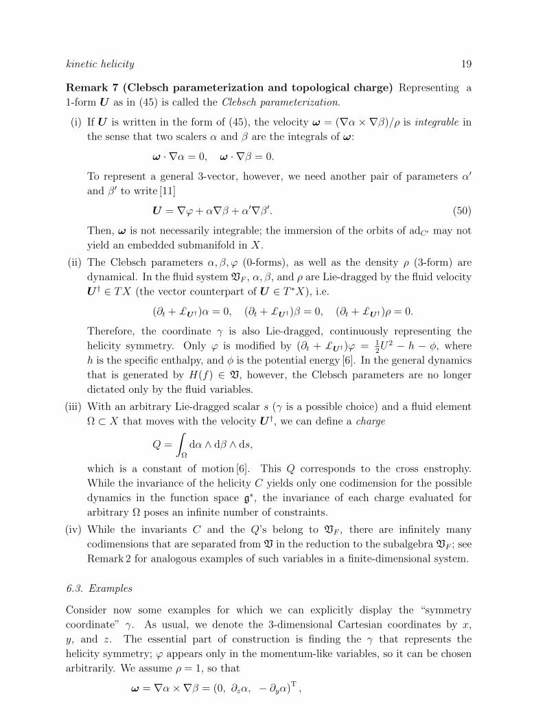
Figure 1. (a) Elliptic vortex ω and the corresponding Gauss potential α (dotted

lines show the level-sets). (b) The relation between the coordinates α (blue dotted)

and γ (black).

and find that α is the Gauss potential of the 2-dimensional vector (ωy, ωz)T on the

surface β = constant.

Example 2 (elliptic vortex) A simple example is the ellipse: For positive a and b,

α = ay2

2+ b

z2

2, β = x ⇒ ω = (0, bz, −ay)T .

Solving ω · ∇γ = 1, we obtain

γ =1√ab

tan−1

(√a

b

y

z

).

Figure 1 shows (a) the contours of α and the vector ω, and (b) the coordinates α (blue

dotted lines) and γ(y, z) (black straight lines). Only when a = b (i.e. the circular vortex)

are α and γ orthogonal to each other. The other coordinate β = x is orthogonal to both

α and γ.

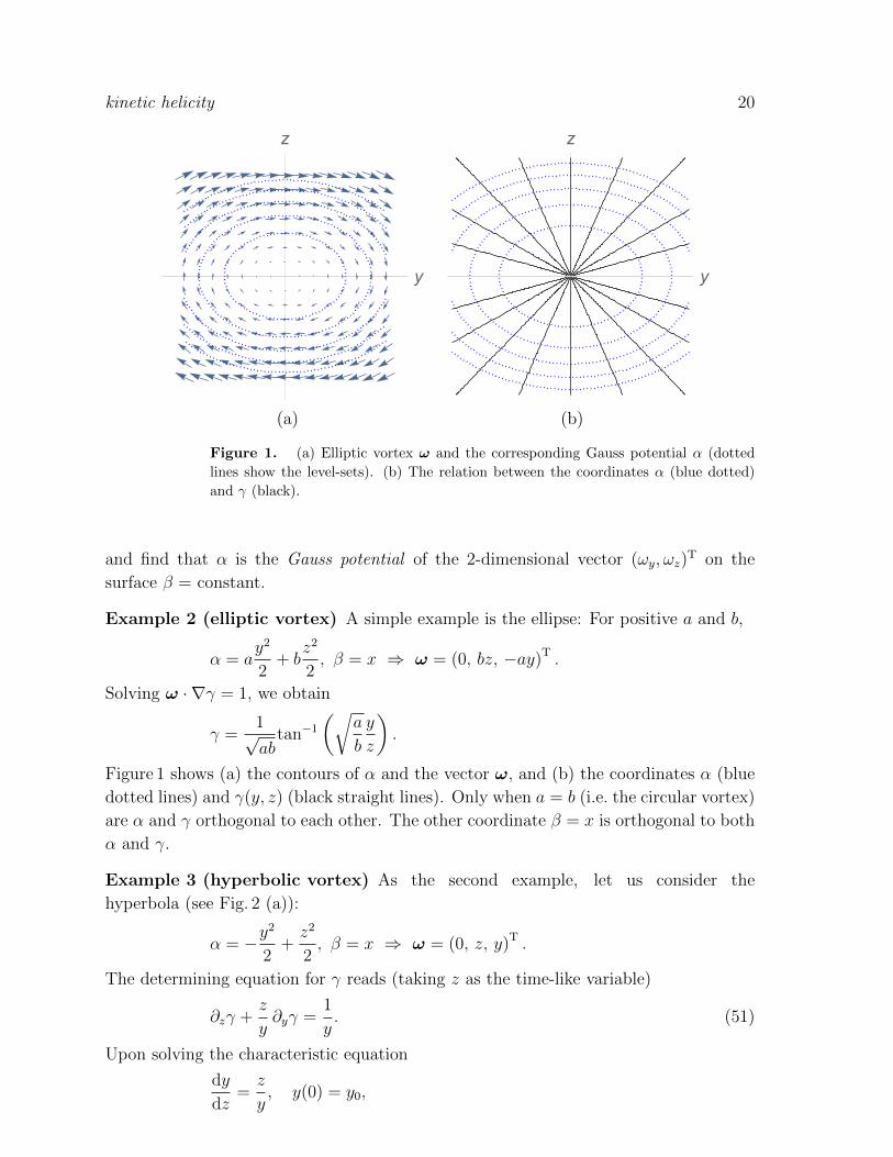
Example 3 (hyperbolic vortex) As the second example, let us consider the

hyperbola (see Fig. 2 (a)):

α = −y2

2+z2

2, β = x ⇒ ω = (0, z, y)T .

The determining equation for γ reads (taking z as the time-like variable)

∂zγ +z

y∂yγ =

1

y. (51)

Upon solving the characteristic equation

dy

dz=z

y, y(0) = y0,

kinetic helicity 21

y

z

y

z

(a) (b)

Figure 2. (a) Hyperbolic vortex ω and the corresponding Gauss potential α (dotted

lines show the level-sets). (b) The relation between the coordinates α (blue, dotted)

and γ (g1: black, and g2: orange).

we obtain y(z) = ±√z2 + y2

0, or y0 = ±√y2 − z2. For an intermediate “time” ζ

(z ≥ ζ ≥ 0), we have

y(ζ) = ±√y2 − z2 + ζ2,

by which we can integrate (51) as

γ =

∫ z

0

dζ

y(ζ).

Because the singularities of the integrand separate different branches of the solution, we

first invoke the indefinite integral:

g(y, z; ζ) =

∫dζ

y(ζ)

=1

2

[log

(1 +

ζ

y(ζ)

)− log

(1− ζ

y(ζ)

)]. (52)

Evaluating g(y, z; ζ) at ζ = z, and setting the “initial time” at ζ = 0, we obtain

γ = γ1 = g(y, z; ζ)|z0 = ±1

2

[log

(1 +

z√y2

)− log

(1− z√

y2

)].

The characteristic curves that start from z = 0 do not reach the domain z2 > y2;

see Fig. 2 (a). To construct a solution there, we reverse the roles of z and y, and define

characteristics for z|y=0 = z0. By the same procedure, we obtain

γ = γ2 = ±1

2

[log

(1 +

y√z2

)− log

(1− y√

z2

)].

kinetic helicity 22

y

z

y

z

(a) (b)

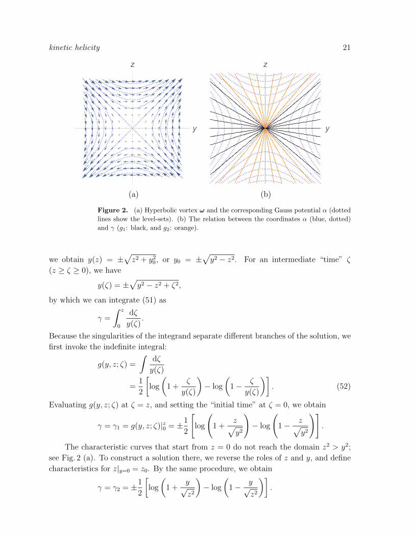
Figure 3. (a) Transformed coordinate g′ = g + α. (b) Transformation obtained by

shifting the lower bound of the integral of (52) to z = −π/2.

These two functions γ1 and γ2 define separate local coordinates in the x-space. Figure 2

shows (a) the contours of α and the vector ω, and (b) the coordinates α (blue dotted

lines) and γ(y, z) (black and orange lines).

Here we note that the solution γ of the determining equation ∇α × ∇β · ∇γ = 1

is not unique. Evidently, the transformation γ 7→ γ + f(α) (f an arbitrary C1

function) produces an infinite set of solutions. Different choices of such transformations

amount to changing the lower-bound of the integral of (52), because g(y, z; c) (c an

arbitrary constant) satisfies ∇α×∇β · ∇g(y, z; c) = 0, i.e., g(y, z; c) = f(α). With the

transformation, the boundaries of the coordinate patches move (see Fig. 3).

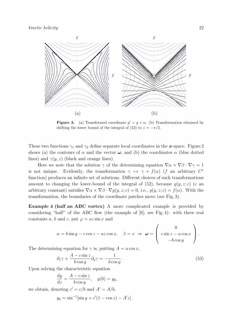
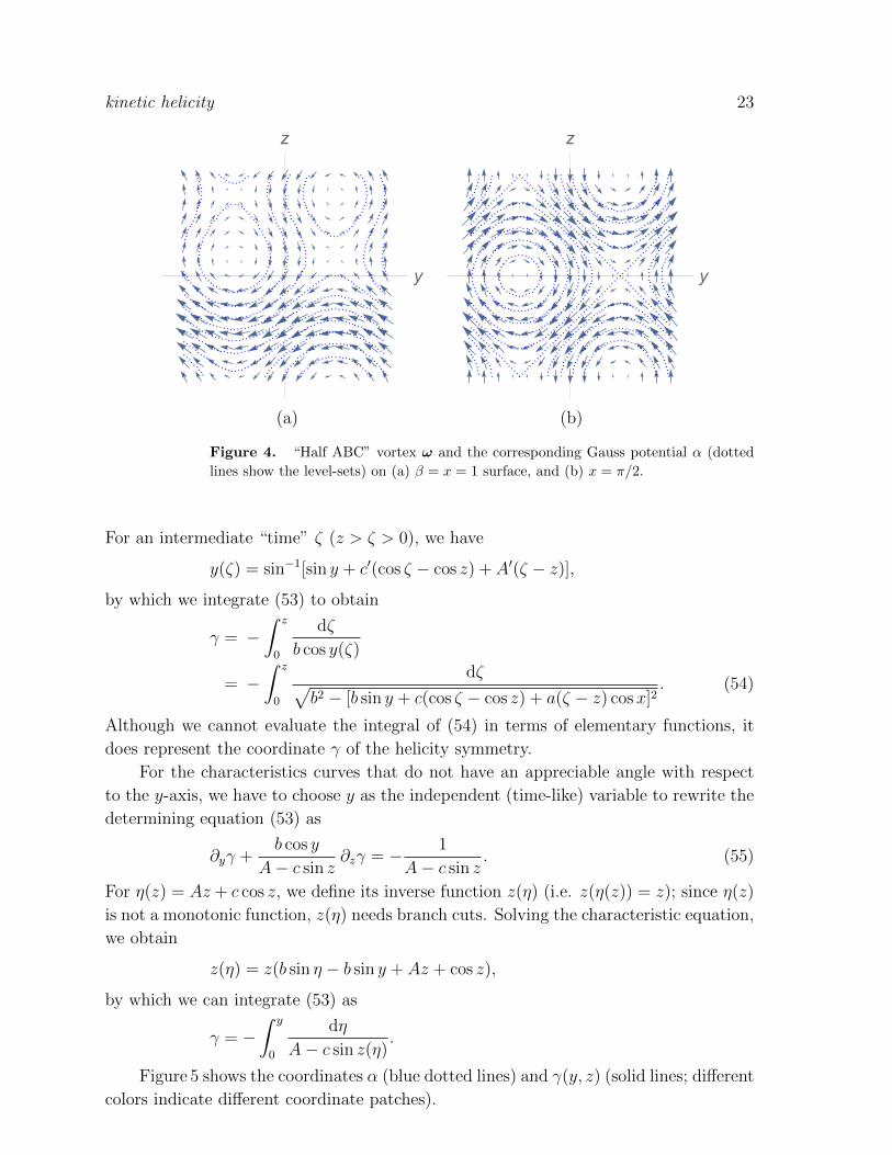
Example 4 (half an ABC vortex) A more complicated example is provided by

considering “half” of the ABC flow (the example of [6]; see Fig. 4): with three real

constants a, b and c, put ϕ = az sinx and

α = b sin y − c cos z − az cosx, β = x ⇒ ω =

0

c sin z − a cosx

−b cos y

.

The determining equation for γ is, putting A = a cosx,

∂zγ +A− c sin z

b cos y∂yγ = − 1

b cos y. (53)

Upon solving the characteristic equation

dy

dz=A− c sin z

b cos y, y(0) = y0,

we obtain, denoting c′ = c/b and A′ = A/b,

y0 = sin−1[sin y + c′(1− cos z)− A′z] .

kinetic helicity 23

y

z

y

z

(a) (b)

Figure 4. “Half ABC” vortex ω and the corresponding Gauss potential α (dotted

lines show the level-sets) on (a) β = x = 1 surface, and (b) x = π/2.

For an intermediate “time” ζ (z > ζ > 0), we have

y(ζ) = sin−1[sin y + c′(cos ζ − cos z) + A′(ζ − z)],

by which we integrate (53) to obtain

γ = −∫ z

0

dζ

b cos y(ζ)

= −∫ z

0

dζ√b2 − [b sin y + c(cos ζ − cos z) + a(ζ − z) cosx]2

. (54)

Although we cannot evaluate the integral of (54) in terms of elementary functions, it

does represent the coordinate γ of the helicity symmetry.

For the characteristics curves that do not have an appreciable angle with respect

to the y-axis, we have to choose y as the independent (time-like) variable to rewrite the

determining equation (53) as

∂yγ +b cos y

A− c sin z∂zγ = − 1

A− c sin z. (55)

For η(z) = Az + c cos z, we define its inverse function z(η) (i.e. z(η(z)) = z); since η(z)

is not a monotonic function, z(η) needs branch cuts. Solving the characteristic equation,

we obtain

z(η) = z(b sin η − b sin y + Az + cos z),

by which we can integrate (53) as

γ = −∫ y

0

dη

A− c sin z(η).

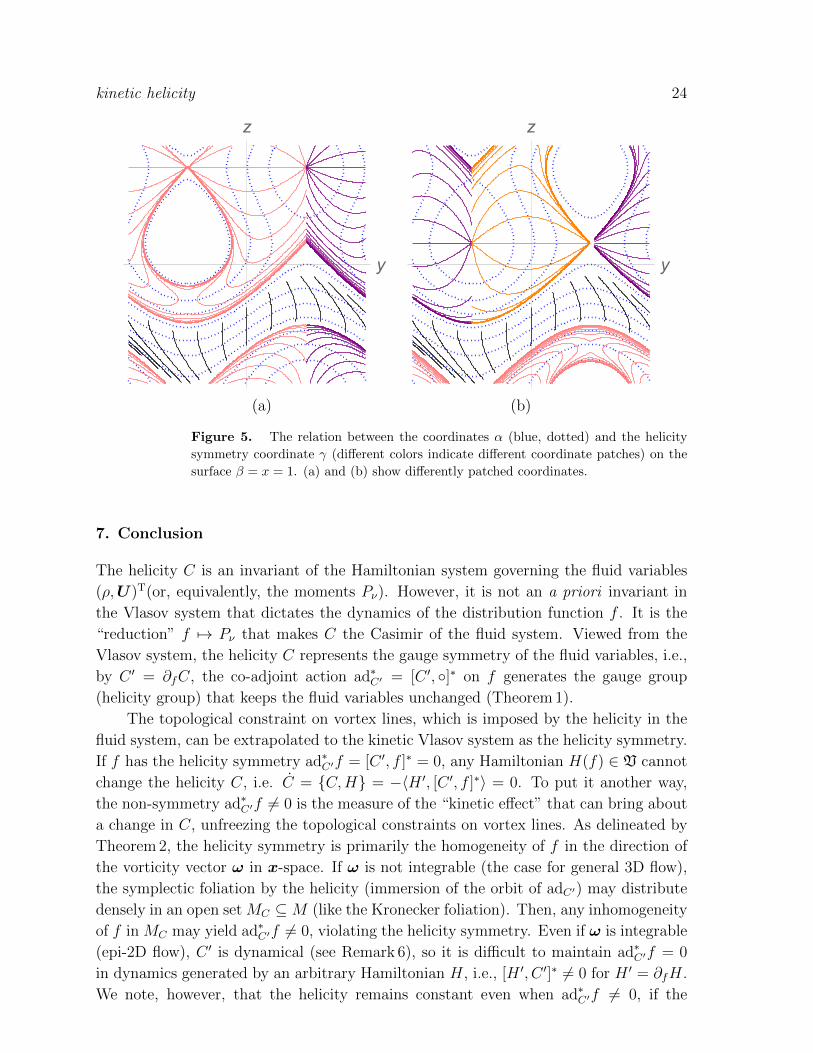
Figure 5 shows the coordinates α (blue dotted lines) and γ(y, z) (solid lines; different

colors indicate different coordinate patches).

kinetic helicity 24

y

z

y

z

(a) (b)

Figure 5. The relation between the coordinates α (blue, dotted) and the helicity

symmetry coordinate γ (different colors indicate different coordinate patches) on the

surface β = x = 1. (a) and (b) show differently patched coordinates.

7. Conclusion

The helicity C is an invariant of the Hamiltonian system governing the fluid variables

(ρ,U)T(or, equivalently, the moments Pν). However, it is not an a priori invariant in

the Vlasov system that dictates the dynamics of the distribution function f . It is the

“reduction” f 7→ Pν that makes C the Casimir of the fluid system. Viewed from the

Vlasov system, the helicity C represents the gauge symmetry of the fluid variables, i.e.,

by C ′ = ∂fC, the co-adjoint action ad∗C′ = [C ′, ]∗ on f generates the gauge group

(helicity group) that keeps the fluid variables unchanged (Theorem 1).

The topological constraint on vortex lines, which is imposed by the helicity in the

fluid system, can be extrapolated to the kinetic Vlasov system as the helicity symmetry.

If f has the helicity symmetry ad∗C′f = [C ′, f ]∗ = 0, any Hamiltonian H(f) ∈ V cannot

change the helicity C, i.e. C = C,H = −〈H ′, [C ′, f ]∗〉 = 0. To put it another way,

the non-symmetry ad∗C′f 6= 0 is the measure of the “kinetic effect” that can bring about

a change in C, unfreezing the topological constraints on vortex lines. As delineated by

Theorem 2, the helicity symmetry is primarily the homogeneity of f in the direction of

the vorticity vector ω in x-space. If ω is not integrable (the case for general 3D flow),

the symplectic foliation by the helicity (immersion of the orbit of adC′) may distribute

densely in an open set MC ⊆M (like the Kronecker foliation). Then, any inhomogeneity

of f in MC may yield ad∗C′f 6= 0, violating the helicity symmetry. Even if ω is integrable

(epi-2D flow), C ′ is dynamical (see Remark 6), so it is difficult to maintain ad∗C′f = 0

in dynamics generated by an arbitrary Hamiltonian H, i.e., [H ′, C ′]∗ 6= 0 for H ′ = ∂fH.

We note, however, that the helicity remains constant even when ad∗C′f 6= 0, if the

kinetic helicity 25

Hamiltonian includes only the fluid variables Pν , because∫Vvνad∗C′f d3v = 0 for every

f (Theorem 1).

Finally, we note the remarkable analogy between the Casimir C and the magnetic

moment µ of a magnetized particle (see Sec. 2.1). The adiabatic invariance of the action

µ is due to the separation of the microscopic gyration angle θ from the Hamiltonian. In

the macroscopic model, the homogeneity of the distribution function with respect to θ

justifies the separation of the action µ and angle θ variable, resulting is the macroscopic

reduced system. Here, the homogenization of f with respect to the co-adjoint orbit of

ad∗C′ = [C ′, ]∗ yields C as an adiabatic invariant; the orbit is in the direction of the

vorticity vector ω in X, accompanied by −£ω(v−U) in V ; see (36) and (37). For an epi-

2D flow, we can write adC′ = ∂γ with conjugate variables C ′ = ℘γ and γ (Theorem 2);

in the analogy of the magnetic moment, γ parallels the gyro angle. As given in (47),

the canonical momenta ℘j (j = α, β, γ) involve the spatial terms −∂jϕ = −iωjU , where

U resembles the vector potential of the electromagnetic field.

Acknowledgments

This material is based upon work supported by the National Science Foundation under

Grant No. 1440140, while the authors were in residence at the Mathematical Sciences

Research Institute in Berkeley, California, during the semester “Hamiltonian systems,

from topology to applications through analysis” year of 2018. The work of ZY was

partly supported by JSPS KAKENHI grant number 17H01177, and that of PJM was

supported by the DOE Office of Fusion Energy Sciences, under DE-FG02-04ER- 54742

and a Forschungspreis from the Alexander von Humboldt Foundation. He warmly

acknowledges the hospitality of the Numerical Plasma Physics Division of Max Planck

IPP, Garching, Germany, where a portion of this research was done.

References

[1] P. J. Morrison, Hamiltonian description of the ideal fluid, Rev. Mod. Phys. 70 (1998) 467–521.

[2] Z. Yoshida and P. J. Morrison, A hierarchy of noncanonical Hamiltonian systems: circulation laws

in an extended phase space, Fluid Dyn. Res. 46 (2014) 031412 (21pages).

[3] J. Marsden and A. Weinstein, Reduction of symplectic manifolds with symmetry, Rep. Math. Phys.

5 (1974) 121–130.

[4] P. J. Morrison and J. M. Greene, Noncanonical Hamiltonian density formulation of hydrodynamics

and Ideal magnetohydrodynamics, Phys. Rev. Lett. 80 (1980) 790–794.

[5] K. H. Moffatt, The degree of knottedness of tangled vortex lines, J. Fluid Mech. 35 (1969) 117–129.

[6] Z. Yoshida and P. J. Morrison, Epi-two-dimensional fluid flow: A new topological paradigm for

dimensionality, Phys. Rev. Lett. 119 (2017) 244501 (5pages).

[7] P. J. Morrison, The Maxwell-Vlasov equations as a continuous Hamiltonian system, Phys. Lett. A

80 (1980) 383–386.

[8] P. J. Morrison, Poisson brackets for fluids and plasmas AIP Conf. Proc. 88 (1982) 13–46.

[9] P. J. Morrison, N. Lebovitz, and J. Biello The Hamiltonian description of incompressible fluid

ellipsoids Ann. Physics 324 (2009) 1747–1762.

kinetic helicity 26

[10] S. Meacham, P. J. Morrison, and G. Flierl, Hamiltonian moment reduction for describing vortices

in shear, Phys. Fluids 9 (1997) 2310–2328.

[11] Z. Yoshida, Clebsch parameterization: basic properties and remarks on its applications, J. Math.

Phys. 50 (2009) 113101 (16 pages).