The Kelly Criterion

How To Manage Your Money When You Have an Edge

2

The First Model

• You play a sequence of games• If you win a game, you win W dollars for each

dollar bet• If you lose, you lose your bet• For each game,

– Probability of winning is p– Probability of losing is q =1 –p

• You start out with a bankroll of B dollars

3

The First Model, con’t

• You bet some percentage, f, of your bankroll on the first game --- You bet fB

• After the first game you have B1 depending on whether you win or lose

• You then bet the same percentage f of your new bankroll on the second game --- You bet fB1

• And so on• The problem is what should f be to maximize

your “expected” gain– That value of f is called the Kelly Criterion

4

Kelly Criterion

• Developed by John Kelly, a physicist at Bell Labs– 1956 paper “A New Interpretation of Information Rate”

published in the Bell System Technical Journal• Original title “Information Theory and Gambling”

– Used Information Theory to show how a gambler with inside information should bet

• Ed Thorpe used system to compute optimum bets for blackjack and later as manager of a hedge fund on Wall Street– 1962 book “Beat the Dealer: A Winning Strategy for

the Game of Twenty One”

5

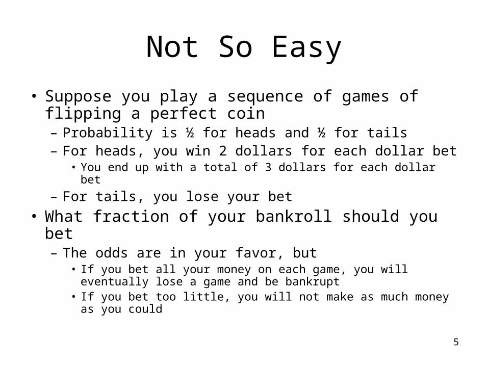
Not So Easy

• Suppose you play a sequence of games of flipping a perfect coin– Probability is ½ for heads and ½ for tails– For heads, you win 2 dollars for each dollar bet

• You end up with a total of 3 dollars for each dollar bet

– For tails, you lose your bet

• What fraction of your bankroll should you bet– The odds are in your favor, but

• If you bet all your money on each game, you will eventually lose a game and be bankrupt

• If you bet too little, you will not make as much money as you could

6

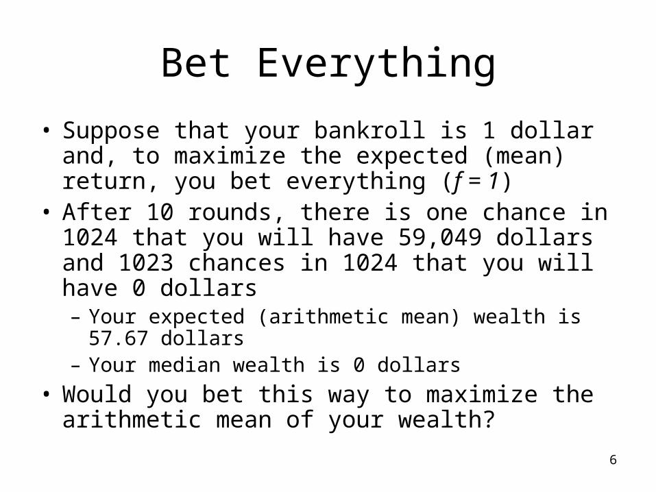
Bet Everything

• Suppose that your bankroll is 1 dollar and, to maximize the expected (mean) return, you bet everything (f = 1)

• After 10 rounds, there is one chance in 1024 that you will have 59,049 dollars and 1023 chances in 1024 that you will have 0 dollars– Your expected (arithmetic mean) wealth is 57.67

dollars– Your median wealth is 0 dollars

• Would you bet this way to maximize the arithmetic mean of your wealth?

7

Winning W or Losing Your Bet

• You play a sequence of games• In each game, with probability p, you win W for

each dollar bet• With probability q = 1 – p, you lose your bet• Your initial bankroll is B• What fraction, f, of your current bankroll should

you bet on each game?

8

Win W or Lose your Bet, con’t

• In the first game, you bet fB– Assume you win. Your new bankroll is

B1 = B + WfB = (1 + fW) B

– In the second game, you bet fB1 fB1 = f(1 + fW) B

– Assume you win again. Your new bankroll is B2 = (1 + fW) B1 = (1 + fW)2 B

– If you lose the third game, your bankroll is B3 = (1 – f) B2 = (1 + fW)2 * (1 – f) B

9

Win W or Lose your Bet, con’t

• Suppose after n games, you have won w games and lost l games– Your total bankroll is

Bn = (1 +fW)w * (1 – f)l B

– The gain in your bankroll is Gainn = (1 + fW)w * (1 – f)l

• Note that the bankroll is growing (or shrinking) exponentially

10

Win W or Lose your Bet, con’t

• The possible values of your bankroll (and your gain) are described by probability distributions

• We want to find the value of f that maximizes, in some sense, your “expected” bankroll (or equivalently your “expected” gain)

• There are two ways we can think about finding this value of f– They both yield the same value of f and, in fact, are

mathematically equivalent • We want to find the value of f that maximizes

– The geometric mean of the gain– The arithmetic mean of the log of the gain

11

Finding the Value of f that Maximizes the Geometric Mean of

the Gain• The geometric mean, G, is the limit as n

approaches infinity of the nth root of the gain G = lim n->oo ((1 + fW)w/n * (1 – f)l/n )

which is G = (1 + fW)p * (1 – f)q

• For this value of G, the value of your bankroll after n games is Bn = Gn * B

12

The Intuition Behind the Geometric Mean

• If you play n games with a probability p of winning each game and a probability q of losing each game, the expected number of wins is pn and the expected number of loses is qn

• The value of your bankroll after n games Bn = Gn * B

is the value that would occur if you won exactly pn games and lost exactly qn games

13

Finding the Value of f that Maximizes the Geometric Mean of

the Gain, con’t• To find the value of f that maximizes G, we take the

derivative of G = (1 + fW)p * (1 – f)q

with respect to f, set the derivative equal to 0, and solve for f

(1 + fW)p *(-q (1 – f)q-1) + Wp(1 + fW)p-1 * (1 – f)q = 0• Solving for f gives

f = (pW – q) / W = p – q / W • This is the Kelly Criterion for this problem

14

Finding the Value of f that Maximizes the Arithmetic Mean of

the Log of the Gain• Recall that the gain after w wins and l losses is

Gainn = (1 + fW)w * (1 – f)l

• The log of that gain is

log(Gainn) = w * log(1 + fW) + l* log (1 – f)

• The arithmetic mean of that log is the

lim n->oo ( w/n * log(1 + fW) + l/n* log (1 – f) )

which is p * log(1 + fW) + q * log (1 – f)

15

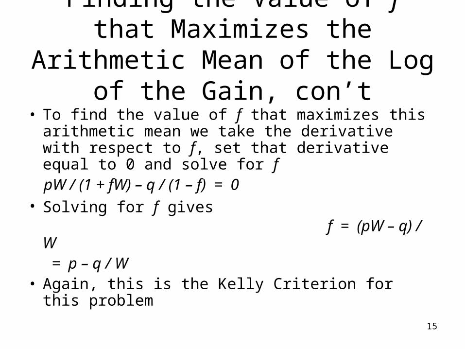
Finding the Value of f that Maximizes the Arithmetic Mean of

the Log of the Gain, con’t • To find the value of f that maximizes this

arithmetic mean we take the derivative with respect to f, set that derivative equal to 0 and solve for f

pW / (1 + fW) – q / (1 – f) = 0• Solving for f gives

f = (pW – q) / W = p – q / W• Again, this is the Kelly Criterion for this problem

16

Equivalent Interpretations of Kelly Criterion

• The Kelly Criterion maximizes – Geometric mean of wealth– Arithmetic mean of the log of wealth

17

Relating Geometric and Arithmetic Means

• Theorem

The log of the geometric mean of a random variable equals the arithmetic mean of the log of that variable

18

Intuition About the Kelly Criterion for this Model

• The Kelly criterion

f = (pW – q) / W is sometimes written as f = edge / odds– Odds is how much you will win if you win

• At racetrack, odds is the tote-board odds

– Edge is how much you expect to win• At racetrack, p is your inside knowledge of which

horse will win

19

Examples• For the original example (W = 2, p = ½) f = .5 -

.5 / 2 = .25 G = 1.0607

– After 10 rounds (assuming B = 1)• Expected (mean) final wealth = 3.25• Median final wealth = 1.80

• By comparison, recall that if we bet all the money (f = 1)– After 10 rounds (assuming B = 1)

• Expected (mean) final wealth = 57.67• Median final wealth = 0

20

More Examples

• If pW – q = 0, then f = 0 – You have no advantage and shouldn’t bet

anything – In particular, if p = ½ and W = 1, then again

f = 0

21

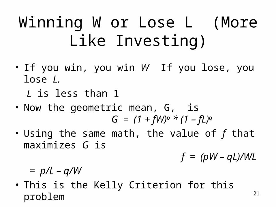
Winning W or Lose L (More Like Investing)

• If you win, you win W If you lose, you lose L.

L is less than 1• Now the geometric mean, G, is

G = (1 + fW)p * (1 – fL)q

• Using the same math, the value of f that maximizes G is f = (pW – qL)/WL

= p/L – q/W• This is the Kelly Criterion for this problem

22

An Example

• Assume p = ½, W = 1, L = 0.5. Then f = .5G = 1.0607

• As an example, assume B = 100. You play two games– Game 1 you bet 50 and lose (25) . B is now 75– Game 2 you bet ½ of new B or 37.50. You win. B is

112.50• By contrast, if you had bet your entire bankroll

on each game, – After Game 1, B would be 50 – After Game 2, B would be 100

23

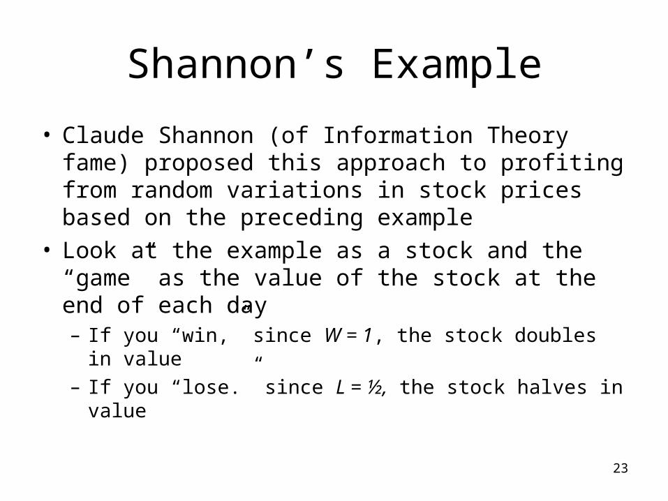
Shannon’s Example

• Claude Shannon (of Information Theory fame) proposed this approach to profiting from random variations in stock prices based on the preceding example

• Look at the example as a stock and the “game” as the value of the stock at the end of each day– If you “win,” since W = 1, the stock doubles in value– If you “lose.” since L = ½, the stock halves in value

24

Shannon’s Example, con”t

• In the example, the stock halved in value the first day and then doubled in value the second day, ending where it started– If you had just held on to the stock, you would have

broken even• Nevertheless Shannon made money on it

– The value of the stock was never higher than its initial value, and yet Shannon made money on it

• His bankroll after two days was 112.50– Even if the stock just oscillated around its initial value

forever, Shannon would be making (1.0607)n gain in n days

25

An Interesting Situation

• If L is small enough, f can be equal to 1 (or even larger)– You should bet all your money

26

An Example of That Situation

• Assume p = ½, W = 1, L = 1/3 . Then

f = 1

G = 1.1547• As an example, assume B = 100. You play two

games– Game 1 you bet 50 and lose 16.67 B is now

66.66– Game 2 you bet 66.66 and win. B is now

133.33

27

A Still More Interesting Situation

• If L were 0 (you couldn’t possibly lose) f would be infinity– You would borrow as much money as you

could (beyond your bankroll) to bet all you possibly could.

28

N Possible Outcomes (Even More Like Investing)

• There are n possible outcomes, xi ,each with probability pi

– You buy a stock and there are n possible final values, some positive and some negative

• In this caseip

ifxG )1(

29

N Outcomes, con’t

• The arithmetic mean of the log of the gain is

• The math would now get complicated, but if fxi << 1 we can approximate the log by the

first two terms of its power expansion

to obtain

)1log(*log ii fxpGR

2/log 22iiii xpfxpfGR

...4/3/2/)1log( 432 zzzzz

30

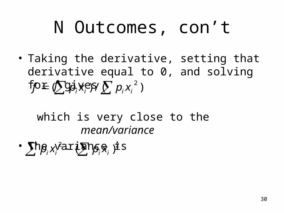
N Outcomes, con’t

• Taking the derivative, setting that derivative equal to 0, and solving for f gives

which is very close to the mean/variance

• The variance is

)/()( 2iiii xpxpf

22 )( iiii xpxp

31

Properties of the Kelly Criterion

• Maximizes – The geometric mean of wealth– The arithmetic mean of the log of wealth

• In the long term (an infinite sequence), with probability 1– Maximizes the final value of the wealth (compared

with any other strategy)– Maximizes the median of the wealth

• Half the distribution of the “final” wealth is above the median and half below it

– Minimizes the expected time required to reach a specified goal for the wealth

32

Fluctuations using the Kelly Criterion

• The value of f corresponding to the Kelly Criterion leads to a large amount of volatility in the bankroll– For example, the probability of the bankroll dropping

to 1/n of its initial value at some time in an infinite sequence is 1/n

• Thus there is a 50% chance the bankroll will drop to ½ of its value at some time in an infinite sequence

– As another example, there is a 1/3 chance the bankroll will half before it doubles

33

An Example of the Fluctuation

34

Varying the Kelly Criterion

• Many people propose using a value of f equal to ½ (half Kelly) or some other fraction of the Kelly Criterion to obtain less volatility with somewhat slower growth– Half Kelly produces about 75% of the growth

rate of full Kelly– Another reason to use half Kelly is that people

often overestimate their edge.

35

Growth Rate for Different Kelly Fractions

36

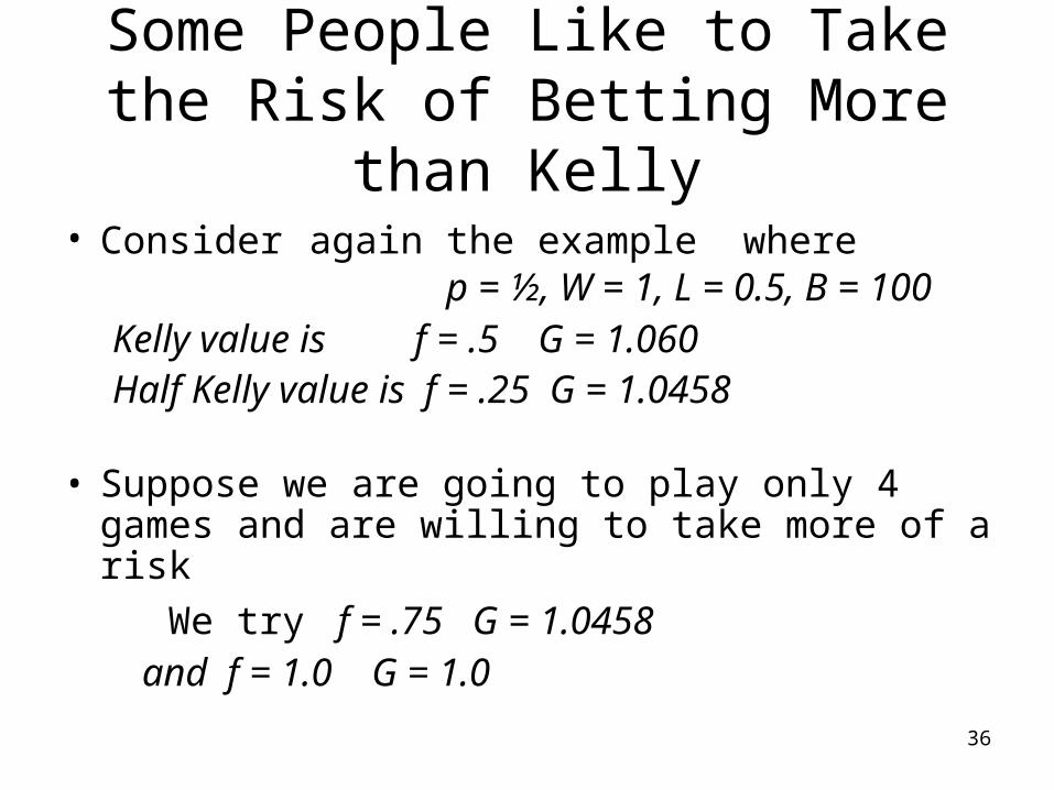
Some People Like to Take the Risk of Betting More than Kelly

• Consider again the example where p = ½, W = 1, L = 0.5, B = 100Kelly value is f = .5 G = 1.060Half Kelly value is f = .25 G = 1.0458

• Suppose we are going to play only 4 games and are willing to take more of a risk

We try f = .75 G = 1.0458 and f = 1.0 G = 1.0

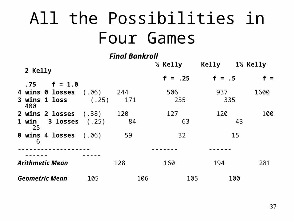
37

All the Possibilities in Four Games

Final Bankroll ½ Kelly Kelly 1½ Kelly 2 Kelly f = .25 f = .5 f = .75 f = 1.04 wins 0 losses (.06) 244 506 937 16003 wins 1 loss (.25) 171 235 335 4002 wins 2 losses (.38) 120 127 120 1001 win 3 losses (.25) 84 63 43 250 wins 4 losses (.06) 59 32 15 6------------------- ------- ------ ------ -----Arithmetic Mean 128 160 194 281

Geometric Mean 105 106 105 100

38

I Copied This From the Web

If I maximize the expected square-root of wealth and you maximize expected log of wealth, then after 10 years you will be richer 90% of the time. But so what, because I will be much richer the remaining 10% of the time. After 20 years, you will be richer 99% of the time, but I will be fantastically richer the remaining 1% of the time.

39

The Controversy

• The math in this presentation is not controversial• What is controversial is whether you should use

the Kelly Criterion when you gamble (or invest)– You are going to make only a relatively short

sequence of bets compared to the infinite sequence used in the math

• The properties of infinite sequences might not be an appropriate guide for a finite sequence of bets

• You might not be comfortable with the volatility– Do you really want to maximize the arithmetic mean

of the log of your wealth (or the geometric mean of your wealth)?

• You might be willing to take more or less risk

40

Some References• Poundstone, William, “Fortunes Formula: The Untold Story of the

Scientific Betting System that Beat the Casinos and Wall Street,” Hill and Wang, New York, NY, 2005

• Kelly, John L, Jr., A New Interpretation of Information Rate, Bell Systems Technical Journal, Vol. 35, pp917-926, 1956

• http://www-stat.wharton.upenn.edu/~steele/Courses/434F2005/Context/Kelly%20Resources/Samuelson1979.pdf– Famous paper that critiques the Kelly Criterion in words of one syllable

• http://en.wikipedia.org/wiki/Kelly_criterion• http://www.castrader.com/kelly_formula/index.html

– Contains pointers to many other references