The irony of the magnet system for Kibblebalances – a review

Shisong Li1, Stephan Schlamminger2

1. Department of Electrical Engineering, Tsinghua University, Beijing 100084,China2. National Institute of Standards and Technology (NIST), Gaithersburg, 20899MD, United States

E-mail: shisong.li@outlook.com; stephan.schlamminger@nist.gov

Abstract. The magnet system is an essential component of the Kibble balance,a device that is used to realize the unit of mass. It is the source of the magneticflux, and its importance is captured in the geometric factor Bl. Ironically, the Blfactor cancels out and does not appear in the final Kibble equation. Nevertheless,care must be taken to design and build the magnet system because the cancellationis perfect only if the Bl is the same in both modes: the weighing and velocitymode. This review provides the knowledge necessary to build a magnetic circuitfor the Kibble balance. In addition, this article discusses the design considerations,parameter optimizations, practical adjustments to the finished product, and anassessment of systematic uncertainties associated with the magnet system.

Submitted to: Metrologia

arX

iv:2

111.

0777

2v1

[ph

ysic

s.in

s-de

t] 1

5 N

ov 2

021

2

1. Introduction

Today, the Kibble balance [1] is a precision instrument that is used to realize theunit of mass, and it can weigh masses ranging from grams to kilograms. It is one oftwo methods for the primary realization of the mass unit, the other being the X-raycrystal density method (XRCD) [2].

Previously, the Kibble balance was called the watt balance. The communityagreed to the name change to honor the late Dr. Bryan Kibble, who inventedthis measurement technique. Before 2019, the balance was used to determine thePlanck constant, h, utilizing a mass that was traceable to the international prototypekilogram (IPK) as an input quantity. According to Nature [3], in 2012, the wattbalance was one of the six most difficult experiments.

By the end of July 2017, the different measurements of h had convergedsufficiently to initiate the revision of the international system of units, the SI(abbreviation for the French expression Systeme International d’Unites). Based ondata available at that time, final values were calculated for the Planck constant h, theAvogadro constant NA, the elementary charge e, and the Boltzmann constant k [4].The assigned numerical values to these four constants define four of the seven baseunits in the SI [5]. These are the kilogram, the ampere, the mole, and the kelvin.On May 20th, 2019, the revised SI came into effect. Since then, the Kibble balanceand XRCD have replaced the international prototype kilogram as the starting pointof worldwide mass dissemination. Kibble balance experiments are carried out atmany National Metrology Institutes (NMIs) and the Bureau International des Poidset Measures (BIPM), e.g. [6–15].

The principle of the Kibble balance is based on the measurement of the integralof the magnetic flux density B along the coil wire l or the gradient of the coil fluxlinkage Φ over the vertical direction z, the so-called geometrical factor, given by (seeAppendix A)

Bl =∂Φ

∂z=

∫(dl×B)z (1)

in two separated phases. In the weighing phase, the coil is excited by current I. Theelectromagnetic force is adjusted such that it is equal and opposite to the weight ofa test mass,

(Bl)w =mg

I, (2)

where m and g denote the test mass and local gravitational acceleration, respectively.In the velocity phase, the current is removed, and the open coil is connected to a

3

voltmeter with a high input impedance. The Bl factor is measured by moving thecoil along the vertical direction with a velocity v. The quotient of the induced voltageU to the velocity v is equal to Bl as

(Bl)v =U

v. (3)

Ideally and theoretically that is the case, (Bl)w and (Bl)v are the same, and, hence,the right side of equation (2) is equal to the right side of equation (3). Then, aftercrosswise multiplication, the equation of virtual power, also known as the Kibbleequation,

mgv = UI, (4)

is obtained. The Kibble equation can only be obtained if (Bl)w = (Bl)v. At thispoint, it is necessary to reflect on the relative uncertainties that are required. Thebest Kibble balance can measure a 0.5 kg mass with a relative uncertainty just below1× 10−8 [6]. So the question is, can the ratio (Bl)w/(Bl)v be trusted to be one within±1× 10−8? We will scrutinize this assumption in the sections below.

The current in the weighing phase is measured as a voltage drop V on a standardresistor R, i.e. I = V/R. Solving for mass yields,

m =UV

gvR. (5)

The two different electrical measurements, voltage and resistance, can be traced backto quantum effects. The Josephson effect [16] allows to realize a voltage

U =nUfU

KJ

, (6)

with the Josephson constant KJ = 2e/h. Here nU is the number of JosephsonJunctions used (typically between 104 and 105) and fU is the microwave frequencythat is used to irradiate the Josephson junctions (several tens of GHz). For moreinformation, the reader may consult a recent review on Josephson voltage standards,for example [17].

The standard resistor is compared against, read: “is a fraction η of”, the quantumHall value [18,19],

R = ηRK, (7)

with the von Klitzing constant RK = h/e2. Recent reviews of the quantum Hall effectcan be found in [20,21].

4

Using nV and fV for the corresponding values in the V measurement, equation (5)can be written as

m =nUnV

4η

fUfV

gvh. (8)

The quantum aspects pertain to the electrical measurement chain employed inthe Kibble balance. These aspects are crucial in bridging the gulf between classicaland quantum mechanics [22], and are the prime connection that enables the Kibblebalance to realize the unit of mass. Despite the fact that quantum mechanicsplays a critical role in the Kibble balance, this article focuses on classical physics:the electromechanical transducer. Hence, equation (5) suffices to understand ourconsiderations.

The Kibble balance would not work without a magnet system. Its importance isvisible in the individual measurements made in weighing, (Bl)w, and velocity mode,(Bl)v. In the final equation, i.e., the Kibble equation (5), however, the geometricfactor drops out, and it seems the result is independent of Bl. So, why spend energyand effort designing a perfect magnet system? Because, as we shall see in the nextparagraph, the Bl does matter.

According to equation (5), the obtained value for the mass, m, is given byfive measurements. To find the lowest possible uncertainty for a Kibble balanceexperiment, a simple uncertainty propagation is performed. The relative uncertaintyin the mass, neglecting correlations, is given by(σm

m

)2

=(σv

v

)2

+

(σg

g

)2

+(σR

R

)2

+(σU

U

)2

+(σV

V

)2

, (9)

where σX denotes the absolute uncertainty in the measurement of quantity X. Itis reasonable to assume the same uncertainties for the two voltage measurements,σU = σV. Following the derivation in [23], we replace U with Blv and V withmgR/(Bl) and obtain(σm

m

)2

=(σv

v

)2

+

(σg

g

)2

+(σR

R

)2

+

(1

Bl

)2 (σU

v

)2

+ (Bl)2

(σU

mgR

)2

. (10)

The first three terms in the sum on the right are independent of Bl. The fourth termis inversely proportional to (Bl)2 and the last term proportional to (Bl)2.

To minimize the relative uncertainty in the mass, one has to maximize Bl

according to the fourth term and minimize Bl per the fifth term. This dilemma

5

101 102 103 104 10510−9

10−8

10−7

10−6

Kibble balance measurement capacity

m

v, g,R

V U

weighing measurementvelocity measurement

Bl/(Tm)

Relat

iveun

certa

inty

Figure 1. The relative measurement uncertainty for mass as a function of thechosen Bl, according to equation (10). In this example, σv/v = σg/g = σR/R =

5×10−9, σU = 5 nV, v = 2 mm/s, mgR = 1000 ΩN. The smallest relative uncertaintyof 1× 10−8 is obtained at (Bl)op ≈ 700 Tm [23].

provides the designer with an opportunity. There must be an optimal Bl thatminimizes the relative uncertainty of the mass. It is given by,

(Bl)op =

√mgR

v. (11)

Figure 1 shows the relative uncertainty of the mass as a function of Bl. The graphis obtained for typical parameters of a Kibble balance, m = 1 kg, R = 100 Ω, andv = 2 mm/s. The uncertainties are assumed to be σv/v = σg/g = σR/R = 5 × 10−9,σU = 5 nV. For these parameters, the minimum is achieved at (Bl)op ≈ 700 T m. Notethat (Bl)op only depends on the parameters and not their uncertainties. Furthermore,(Bl)op is proportional to the square root of the product of weight and resistance,√mgR. One can achieve the same performance by scaling both quantities inversely

to each other. Using the same magnet system with m = 100 g and R = 1 kΩ willproduce the same relative uncertainty as if it were used with m = 1 kg and R = 100 Ω.This scaling is only true for the magnet system. The weighing system may have adifferent requirement for smaller and larger masses.

Since Bl is a product, the magnet designer can fix one factor and adjust theother to achieve the desired value. But what is the best strategy? Should the designerincrease B or l to obtain the highest possible value? Or is a trade-off the best strategy?A quantity to consider for this decision is the resistive loss in the coil in the weighing

6

mode P = RcI2, with Rc denoting the coil resistance. With the mass of test mass m,

the optimal Bl and ρ, the wire resistance per unit length, the electrical loss can bewritten in two ways

P =ρm2g2

(Bl)2op

× l =ρm2g2

(Bl)op

× 1

B. (12)

Both formulas have a factor that only depends on the product (Bl)op, ρ, and m. Butthe second-factor changes with the free parameter. The equations show that a largeflux density, and hence a small l, is desired because this scenario leads to a decreasein the power dissipation in the wire. The opposite is true for increasing the length ofthe wire. It would increase the electrical power dissipated in the coil. Consequently,it’s best to make B as large as possible and therefore l as small as possible.

We described how to choose a value for Bl and how to divide it up to B and l,but still unclear is the magnetic flux source. While this topic is discussed in greaterdetail in section 3, a brief overview is given here.

Through the history of the Kibble balance, the source of the magnetic fieldevolved. The predecessor of the Kibble balance, the Ampere balance [24, 25], usedair-cored coils to produce the magnetic flux. These coils were wound with copperwire, and not superconductor wire. We refer to such coils as conventional coils, asopposed to super-conducting coils. The Ampere balance was used to realize theunit of electrical current from 1948 to 1990. Because of the similarity to the Kibblebalance, the magnet system of the Ampere balance can be analyzed within the sameframework, see section 3.1. The conventional coils cannot produce a strong magneticfield. The magnetic flux density at the measurement position was only a few mT,which limited the weighing capacity to a few grams. Although the wire length l orexcitation current can be increased to reach a higher force. In both cases, the self-heating increases which yields to larger uncertainty components caused by adverseeffect of the heating, consistent with equation (12).

Later, different magnetic systems, such as permanent magnet systems [26–28],superconducting coils [29], yoke-based electromagnet [30] were designed to increasethe magnetic field B and, at the same time, reduce the ohmic dissipation. Duringthis time, researchers developed concepts for improving the field profile, e.g. [9,31–33].After more than a decade of iterations, the designs finally converged on the yoke-basedpermanent magnet system [34,35]. The success of the yoke-based permanent magnetsystem relies on two advantages over other designs. First, the yoke can provide awell-defined boundary condition in both radial and azimuthal directions. In this

7

case, the magnetic field design is greatly simplified from a complex three-dimensionalproblem to a one-dimensional optimization. Second, the permanent magnet systemdoes not contain components that must be powered. Instead, the rare-earth magneticmaterial is magnetized during production and remains magnetized for the lifespanof the experiment. Hence, such a system provides the magnetic flux with reducedcomplexity (no power supplies needed) and maintenance cost. The different types ofmagnet systems are reviewed in more detail in section 3.

Yoke-based permanent magnets supply an intense, uniform, and stable magneticfield for Kibble balance measurement. Hence, these days they are the workhorse forKibble balances. Various designs for magnet systems exist, and each magnet systemhas different design parameters that can be optimized. Section 4 discusses the mostimportant considerations for the magnet designer. Among the topics discussed are theselection of the dimensions and the materials for the magnet system. The reader canfind tips regarding the assembly, manufacturing, and final evaluation of the magnetsystem.

Sometimes, the field profile of the assembled magnet is not satisfactory, andadjustments must be made. Section 5 discusses how to shim the magnet to achievethe desired profile. It further details different techniques to characterize the magnetsystem.

Even a perfect magnet will have contributions to the uncertainty budget of theKibble balance. There will always be imperfections. The magnetic field will never beperfectly symmetric. Furthermore, magnetic materials are inherently nonlinear, andnonlinear effects can bias the measurement. The text in section 6 discusses the majormagnetic systematic concerns for different measurement schemes.

2. Brief review of the physics of magnetic fields

This section aims to make the reader familiar with the terminology used for the designof static magnetic fields. We introduce the symbols and show basic formulas typicallyused in textbooks about the subject. A reader that is familiar with the topic mayskip this section.

2.1. The magnetic flux density

The most used quantity in the context of the article is the magnetic flux density B.It is a vectorial quantity ~B. If only the scalar is printed, the magnitude of the vector

8

is indicated B = | ~B|. The magnetic flux density is a source-free vector field. Thatmeans the field lines have neither beginning nor end. They are closed. Maxwell’ssecond equation describes this fact. It says that the divergence of the magnetic fluxdensity is 0, ~∇ · ~B = 0.

In Cartesian coordinates, ~B has the components Bx, By, and Bz along thethree coordinate vectors ~ex, ~ey, and ~ez. However since most coils are wound ona circular former it is often more convenient to use cylindrical coordinates, ~B =

Br~er + Bϕ~eϕ + Bz~ez, where r, ϕ and z are the cylindrical coordinates, and ~er, ~eϕ, ~ez

are the corresponding unit vectors.In cylindrical coordinates, the divergence of ~B is given by

~∇ · ~B =1

r

∂(rBr)

∂r+

1

r

∂Bϕ

∂ϕ+∂Bz

∂z= 0. (13)

This result leads to an important corollary. If the flux density has cylindricalsymmetry, that is, it is independent of the azimuth ϕ, then

Br

r+∂Br

∂r= −∂Bz

∂z. (14)

If, furthermore, the radial component of the field is inverse proportional to r, that is,Br = Bcrc/r, then ∂Bz/∂z = 0. Here, Bc is the radial field at the mean radius of thecoil rc, Br(rc) = Bc. For such a field, the vertical component of B does not changewith z.

2.2. The magnetic field

The magnetic field is abbreviated with ~H. In a vacuum, ~H is except a factor, namedthe vacuum permeability, the same as ~B. It is ~H = µ−1

0~B. Inside matter, however,

the two vectorial quantities differ. The magnetization of the material decreases themagnetic field, ~H = µ−1

0~B− ~M . Inside a permanent magnet, for example Samarium-

Cobalt, the ~B and ~H are in opposite directions. The H field is an important quantityto analyze magnetic circuits. Integrating ~H along a closed path yields∮

~H · d~l = It, (15)

where It is the total current flowing through the surface enclosed by the path.Equation (15) makes it easy to remember that the unit of H is A/m. A typicalcase here is the analysis of a magnetic circuit without current in the coil. In this case,the enclosed integral evaluates to zero.

9

lm

la

PM yokeyoke

battery (PM)

wire

(yok

e)

wire

(yok

e)

load (air gap)

(a)

(b)

Figure 2. (a) is a simple magnetic circuit with a permanent magnet (PM) andan air gap. The red line denotes a major magnetic flux line through the circuit.(b) shows an equivalent electrical circuit for understanding the magnetic circuit,where the permanent magnet, yoke, and air gap are turned into the battery (withan internal resistance), wire resistance, and load reluctance, respectively.

2.3. The magnetic circuit

A very simple magnetic circuit is shown in figure 2(a). It shows a permanent magnetof width lm, an iron yoke, and an air gap of width la. The red line is the closedcontour over which the integral in equation (15) is calculated. There is no currentenclosed inside the contour and no external magnetic flux is considered, hence, theintegral must evaluate to zero. We can split the path along the contour into threeregions, the permanent magnet, the iron yoke (length ly), and the air gap. In the airgap ~H = µ−1

0~B. In the iron, ~H = (µ0µr)

−1 ~B (µr is the yoke relative permeability)and finally, in the magnet, we have Hm. The complete integral is

Hmlm +By

µ0µr

ly +Ba

µ0

la = 0. (16)

If the cross-sectional areas in the air gap and the yoke and the magnet are the same,a single symbol S is enough to denote this area. In this case, B is identical in the

10

magnet, the yoke, and the air gap, because the flux Φ = BS is conserved. Note, forsimplicity we ignore fringe fields here. It is B = By = Ba = Bm. Equation (16) cannow be easily solved for B, it is

B =−Hmlmlyµ0µr

+laµ0

. (17)

The next question we would like to investigate is: What is the magnetomotiveforce of permanent magnet material? Can it be doubled by doubling the length ofthe magnet? As we shall see, it is not that simple. As the black curve in figure3 shows, commonly used modern magnet materials, e.g., Samarium Cobalt (SmCo)and Neodymium-Iron-Boron (NdFeB), show a linear behavior in the second quadrant(positive B, negative H). The magnetic flux is given by

B = µmµ0H +BR or B = µmµ0(H −HC), (18)

where µm is the relative permeability of the permanent magnet, BR its remanenence,which is the magnetic flux in the absence of H, and HC the coercivity. Note thatBR = −µmµ0HC. Applying

Hm =B

µmµ0

− BR

µmµ0

=B

µmµ0

+HC (19)

into equation (16) and using Φ = SB yields,

Φ

(lm

Sµmµ0

+ly

Sµ0µr

+laSµ0

)=

BR

µmµ0

lm = −HClm. (20)

Besides using Ampere’s law, Ohm’s law in magnetism can be used to understandthe magnetic circuit and derive (20). Similar to Ohm’s law, I = U/R, the magneticversion is as

Φ =F

R, (21)

where R is the magnetic reluctance of the circuit, F the magnetomotive force (MMF).The magnetomotive force corresponds to the voltage (electromotive force, EMF), theflux to the current, and the reluctance to the resistance in the original law by Ohm.The MMF is supplied by the permanent magnet and is given by F = −HC lm. Whilethe reluctances of three components form a serial circuit and add R = Ra +Ry +Rm.The individual reluctances of the air gap, the yoke and the permanent magnet, are

Ra =laSµ0

, Ry =ly

Sµ0µr

, Rm =lm

Sµ0µm

, (22)

respectively. Equation (20) is obtained by replacing R by the sum, of the componentsin equation (22) and F by −HC lm.

11

−1750 −1500 −1250 −1000 −750 −500 −250 00.0

0.2

0.4

0.6

0.8

1.0

1.2

H/(kA m−1)

B/T

orµ0M

/T

µ0MB

HC

BR

Figure 3. Measured demagnetization curve, i.e., the part of the magnetic hysteresisthat is in the second quadrant, for a SmCo sample [33]. The sample was measuredat 26 °C. B = µ0H+µ0M . Since the magnetization changes by less then 10% for Hranging from −800 kA m−1 to 0 A m−1, the magnetic flux density is almost a linearfunction of H in this range.

The following points are helpful when using Ohm’s law to design or analyze amagnet system:

(i) The reluctance of the yoke is very low because the relative permeability of iron,µr is very high, of order 1× 103 or even larger. So, Ry << Ra and Ry << Rm,and hence R ≈ Ra +Rm. The yoke in the magnetic circuit plays a similar role tothe wire in the electric circuit. It guides the flux with very low reluctance, justas the wire in an ideal electrical circuit is thought to have negligible resistance.

(ii) The permanent magnet corresponds to the voltage source (battery) as shown infigure 2(b). The MMF supplied is F = −HClm. However, the magnet comeswith its own reluctance Rm, similar to the internal resistance in a voltage source.

(iii) With the last two items, the effect of doubling the length of the active magneticmaterial on the flux can be analyzed. the flux is

Φ′ =2F

2Rm +Ra

< 2F

Rm +Ra

= 2Φ. (23)

A longer permanent magnet increases the MMF, but also the total reluctance.Hence the flux increase is smaller than proportional to the length. In the limitRa << Rm, the magnetic flux remains constant and does not change withincreasing lm.

12

(iv) The load in the electric circuit corresponds to the air gap in the magnetic circuit.Typically, it has the largest reluctance in the circuit, given by Ra. The ratio ofthe reluctances is proportional to the length ratios (assuming identical area),

Rm

Ra

≈ lmla, (24)

because the relative permeabilities of rare earth magnets are close to one. Whilefor some electrical circuits, the internal resistance of the source can be neglected,the same is not true for magnet systems.

2.4. The magnetic reluctance

Above, we have already used the equation for the reluctance of an element with across-sectional area Sx, flux path length (thickness) of lx, and a relative magneticpermeability µx is

Rx =lx

µ0µxSx

. (25)

Equation (25) has a similar form as the resistance of a conductive block with thesame geometrical parameters (lx, Sx), i.e. R = ρ lx/Sx. To obtaine the equationfor the magnetic reluctance one has to replace the resistivity ρ by the permeability1/(µxµ0).

Designing a magnet for a Kibble balance, very often one has to work withcylindrical gaps, inner radius ri, outer radius ro and height ha. For such a gap,the reluctance is

Ra =1

µ0µaha2πlnro

ri

≈ δ

µ0µaha2πri

, (26)

where the approximation is a Taylor expansion of the natural logarithm for ro = ri +δ

and δ << ri.

2.5. The magnetic force required to split the magnet

In some magnet systems, the coil is surrounded by the yoke. In other words, theair gap is inside the magnet with a few access holes that allow the coil suspensionand laser beams to penetrate. The advantage of such an internal air gap is that thecoil is shielded from fluctuating environmental magnetic fields. The disadvantage isthat the magnet needs to be taken apart to insert the coil. This process is known as“splitting the magnet.”

13

(a) Magnet open (b) Magnet closed

Figure 4. An example of a magnet splitter. (a) and (b) show the open and closestatus, respectively. Reproduced from [33].

An important parameter to design a magnet splitter is the size of the force thatis required to split the magnet. Figure 4 shows a rendering of such a device that isneeded to open the magnet.

The Maxwell stress tensor provides a simple method to calculate the force thatacts on an object in a given space [36]. The force is given by the surface integral,

F =

∮T · dS. (27)

The nine components of the Maxwell stress tensor T are given by

Tij =1

µ0

(BiBj −

1

2δij|B|2

), (28)

where i and j indicate the three directions of the Cartesian coordinates, x, y, and z,or a permutation depending on how the problem is set up. The symbol δij denotesthe Kronecker delta, which is δij = 1 for i = j and δi,j = 0 for i 6= j.

An example of a force calculation using eq. (27) is given in section 4.5.

3. Evolution of different magnet systems

Before discussing the short historical evolution of magnet systems in Kibble balance,we would like to put forward three generally accepted properties that these magnetsystems should have.

(i) The magnet system shall provide a large and uniform magnetic flux densitythroughout the coil at the weighing position and in the volume that the coiltraverses in velocity mode.

14

(ii) The total magnetic flux penetrating the coil and its gradient shall be independentof external (environmental) and internal factors, most importantly, the coilcurrent.

(iii) Manufacturing, operation, and maintenance shall be simple and if possible,economical.

Today, when Kibble’s idea is almost half a century old, the thinking on themagnet system has clarified enough that these three points may sound trivial.Historically, however, that has not always been the case. As is shown below,researchers were reluctant to introduce iron to the magnet system out of worry thatthe nonlinear effects may compromise Kibble’s idea. For the remainder of the text,we will use the three points above to evaluate various types of magnet systems.

3.1. Conventional coil system

Long before the Kibble balance, a different type of electrical balance was used inmetrology to define the unit of current, the ampere. In the international system ofunits that was valid until 20th May 2019, the ampere was defined as the constantcurrent that would produce a force of 2× 10−7 N m−1 between two straight parallelconductors placed one meter apart. In the formal definition, these conductors havenegligible cross-section and extend to infinity. This definition links the only electricalunit in the SI to the mechanical unit via the force between two current-carryingwires. The practical realization of the unit of current was carried out with an Amperebalance, sometimes also referred to as current balance or magnetometer [34].

In the Ampere balance, the force between a fixed and a movable coil connectedto a balance was measured [24, 25]. The electromagnetic force between the two coilscan be written as

F =∂M

∂zIFI = (Bl)wI, (29)

where IF and I are the currents through the fixed and movable coils, respectively.Here, M is the mutual inductance of two coils and ∂M/∂z the gradient of M alongthe vertical direction z. Note, (∂M/∂z)IF is identical to the geometric factor Bl.

The four panels in figure 5 show typical coil configurations used in Amperebalances. Each configuration requires three coils. The difference is whether one coilor two coils are stationary and, correspondingly, two coils or one coil are moving. Thecoils in the pair whether they are moving or not, have identical parameters (diameterand number of turns) but are connected in serial opposition. In the left column of

15

figure 5 the fixed coil assembly is the coil pair, and in the right column, it is the singlecoil. The second choice is which coil assembly has a smaller radius. In the top row offigure 5 the fixed coil assembly is on the inside (smaller radius), whereas in the secondrow, it is on the outside (larger radius). Interestingly, as long as the inner radii, outerradii, and coil separation do not change, all four configurations produce the same Bl,shown in the last row of figure 5. The fact that the four configurations produce thesame Bl can be seen by writing the mutual inductance as a sum of the inductancesbetween the single-coil (S) and two other individual coils (upper U and lower L), i.e.M(z) = MSU(z) −MSL(z). If the mutual induction of one inner and one outer coilas a function of vertical separation is given by M1(z), then MSU(z) = M1(d/2 − z)

and MSL(z) = −M1(d/2 + z). Hence, M(z) = M1(d/2− z) +M1(d/2 + z), and mostimportantly M(z) = M(−z).

One merit of these coil systems is that the field gradient is zero at the symmetryplane, z = 0, since ∂2M/∂z2|z = − ∂2M/∂z2|−z, it follows that ∂2M/∂z2|z=0 = 0.Typically, z = 0 is chosen as the weighing point. Then, the magnetic force F isindependent of small variations of the vertical position of the movable coil. The secondbenefit of this position is that the magnetic flux density is inversely proportional tothe radius, B(r) ∝ r−1. In an azimuthally symmetric geometry, as is discussedhere, B(r) ∝ r−1 leads to an important consequence. The magnetic flux density isdivergence-free, ~∇ · ~B = 0, and hence ∂Bz/∂z = −1

r∂(rB)/∂r. The term to the right

of the equal sign is identical to zero for B(r) ∝ r−1, and, therefore, ∂Bz/∂z = 0.So, no magnetic flux is threading through the coil. This condition is true for theentire plane where B(r) ∝ r−1, in this case, z = 0. The flux through the coil iszero independent of coil radius and horizontal position. That means, in weighing,the result is to first-order independent of the precise horizontal position and the coilradius [24, 37]. The latter can change slightly due to ohmic coil heating. The Blconservation of a r−1 field is further detailed in Appendix B. In summary, takingadvantage of the symmetry at z = 0 makes the measurement less susceptible to smalldeviations from the ideal system.

A magnet system employed for Kibble balance measurement should produce aflat field region along z so that when the coil moves with constant velocity, the inducedvoltage stays stable. For current-carrying coil systems, the easiest way to obtain a flatB(z) profile is to adjust the separation of the double coil d and the horizontal distanceof fixed and movable coils, see e.g. [38–40]. In figure 5 (e), we take an example toshow the magnetic profile distributions with different combinations of d and outer

16

−100 −50 0 50 1000.1

0.2

0.3

0.4

0.5

0.6

d = 200mm,r = 150mm

d = 120mm,r = 150mm

d = 160mm,r = 150mm

d=

160

mm

,r=

140

mm

d = 160mm,r = 160mm

z/mm

1 l∂Φ

∂z

/mT

(a) (b)

(c) (d)

(e)

fixedcoil

fixedcoil

movablecoil

fixedcoil

fixedcoil

movablecoil

movablecoil

movablecoil

fixedcoil

movablecoil

movablecoil

fixedcoil

Figure 5. Panels (a)-(d) show four different coils that can be used in the Amperebalances. The inner coil radius and outer coil radius are respectively r0 and r. Thedistance between the coils that form a pair is d. Panel (e) shows the magnetic fieldproduced by the fixed coil arrangement with ampere-turns of each fixed segmentNIF = 200 A. In this case, r0 = 100 mm. Note the small magnitude of the producedflux density.

17

coil radius r (the inner coil radius is fixed at r0 = 100 mm). It can be seen by eitheradjusting d with a fixed r or the opposite (changing r when d is fixed), a flat magneticprofile (in this case, d = 160 mm, r = 150 mm) can be achieved.

Figure 5(e) shows that the magnetic field produced is weak, below 1 mT, evenwith comparably large ampere-turns NIF = 200 A. From the uncertainty relationshipshown in figure 1, the measurement error for the induced voltage is considerable atsmall Bl values. However, choosing a longer wire l to increase the Bl value will alsoenlarge the wire resistance and the ohmic heating. In summary, the weak field that isproduced by conventional coils is a major drawback. And, hence, these systems areno longer in use for Kibble balances.

3.2. Multi-coil magnet system

Ohmic heating in the field generating coils and its adverse effect can be eliminatedby using superconducting wires. Researchers at the National Institute of Standardsand Technology (NIST, USA) developed a superconducting coil system for the third-generation Kibble balance experiment (NIST-3) [41,42]. The NIST-3 superconductingmagnet is shown in figure 6 (a). Two groups of superconducting coils were employedto produce the magnetic field for the measurement. The main solenoids produceda magnetic profile similar to the conventional coil system but with a much largermanetic flux density (sub-Tesla level). Thanks to T.P. Olsen [24], a pair of trimsolenoids were used to compensate for the first order (z2) non-linearities of the mainsolenoids. Compared to systems shown in figure 5, this double-layer design allows aquasi-realization of 1/r field in a much wider range along z. Figure 6 (a) presents atypical NIST-3 velocity measurement result. As is seen, the magnetic profile changesonly by a few parts in 104 over about 100 mm z travel.

Another novel idea implemented in NIST-3 system is that its induction coilconsists of two individual coils. One is movable and connected to the balance.The other is fixed in space. In fact, the fixed coil itself consists of two coils thatformed together with a virtual coil with the same number of turns as the movingcoil. By connecting the moving and the virtually fixed coil in series opposition,the common electromagnetic noise, canceled [33], improving significantly the signal-to-noise ratio. The idea is similar to a humbucker in an electric guitar. Thedouble movable coil shown in figure 5 can achieve a similar feature. The NIST-3superconducting magnet was a successful system. It met the magnetic requirementsfor Kibble balance measurement and produced one of the most precise results for

18

481.3 481.4 481.5

−40

−20

0

20

40

2× 10−4

Bl/(Tm)

z/m

m

31.74 31.75 31.76−10

−5

0

5

10

2× 10−4

B/mT

z/m

m

(a) NIST-3 (b) NIM-1

1⃝

1⃝

2⃝2⃝

3⃝3⃝

4⃝4⃝

5⃝ 5⃝6⃝

6⃝

7⃝

7⃝

100 mm

700 mm

Figure 6. (a) The NIST-3 superconducting magnetic system. The left plot showsa measurement of the magnetic profile in the velocity phase (reproduced from [42]),and the right plot is the spatial arrangement of superconducting solenoids. (b)The permanent-magnet-only system was used in the Joule balance experiment.The left shows the construction of the system, and the right presents the designed(green) and achieved (red) magnetic profiles. Reproduced from [43]. The labeledcomponents in both systems are: 1©–upper main solenoid/magnet ring, 2©–lowermain solenoid/magnet ring, 3©–upper trim solenoid/magnet ring, 4©–lower trimsolenoid/magnet ring, 5©–main movable coil, 6©– upper fixed compensation coil,7©– lower fixed compensation coil.

determining the Planck constant at the time [29, 41, 44]. One major shortcoming ofthe superconducting system is the complexity of the operation. On needs a stablecurrent control for the solenoids and liquid helium to reach the transition temperaturefor the superconductor. For NIST-3 about 250 L of liquid Helium were necessaryfor a week of operation. The second problem is the lack of a defined and stablemetrological surface. Typically, in velocity mode, the velocity of the coil with respectto the magnet needs to be measured. Very often, that measurement is performedinterferometrically with a surface of the magnet providing a mounting surface forthe reference arm. A superconducting coil, however, does not offer easy access to adefined surface. The plane of interest, the magnetic center of the superconductingcoil, is immersed in liquid helium. A possible surface would be the top of the Dewar,but the stability from that surface to the magnetic center of the coil is not great. Forexample, vibration, magnetostrictive forces, and thermal expansion due to a changein Helium level in the Dewar can affect the distance between the top of the Dewar

19

and the center of the coil.A second attempt to improve the field strength and reduce the ohmic heating for

the coil system was undertaken by researchers at the National Institute of Metrology(NIM, China) for the Joule balance experiment [43]. The idea is to replace thefield generating coils with permanent magnets yielding two advantages: 1) the ohmicheating of the field generating coils is removed, and 2) a stronger magnetic field iscreated. The construction of the NIM-1 magnet system and the magnetic profileare shown in figure 6 (b). A flat magnetic profile of about 30 mT over 1 cm wasobtained. Compared to superconducting coils, the permanent-magnet-only systemis simpler and more compact. However, the field strength was several times weakerthan that of the NIST-3 system, and to produce a 4.9 N force (weight of 500 g mass),the ohmic heating caused by the moving coil of 0.7 W was significant. In reality, alarge-volume permanent magnet is challenging to manufacture, and hence the ringsare usually realized by gluing small pieces together. Typically, the field strength ofdifferent parts can vary by as much as 1%, and the magnetization difference canyield unknown field gradients in open circuits, causing misalignment errors. Besides,the remanence of the permanent magnet has a significant temperature coefficient of−3×10−4/K (SmCo magnet) to −10−3/K (NdFeB magnet), without an efficient heatsink, the magnet temperature needs to be well controlled during the measurement.

The magnet systems described above are open. The magnetic flux is not guidedand, therefore, can penetrate the entire room where the Kibble balance is installed.Thus, the following considerations are essential: 1) There will be a vertical fieldgradient at the mass. As a consequence, a considerable magnetization force occurswhen the mass is made from soft magnetic materials, such as stainless steel [45].2) The magnetic flux density at the coil position can be influenced by iron in itsvicinity. Great care has to be taken to avoid iron, and if iron is unavoidable, ithas to be mounted such that it does not move with respect to the magnet system.A change of the relative positions may alter the field profile and cause systematiceffects. To suppress these effects and, at the same time, further increase the fieldstrength, controlling and aligning the magnetic flux path by introducing soft yokesto the permanent magnet system became inevitable.

3.3. Flat permanent magnet system

The first yoke-based permanent magnet system was employed by the first generationKibble balance experiment (NPL-Mark I) at the National Physical Laboratory (NPL,

20

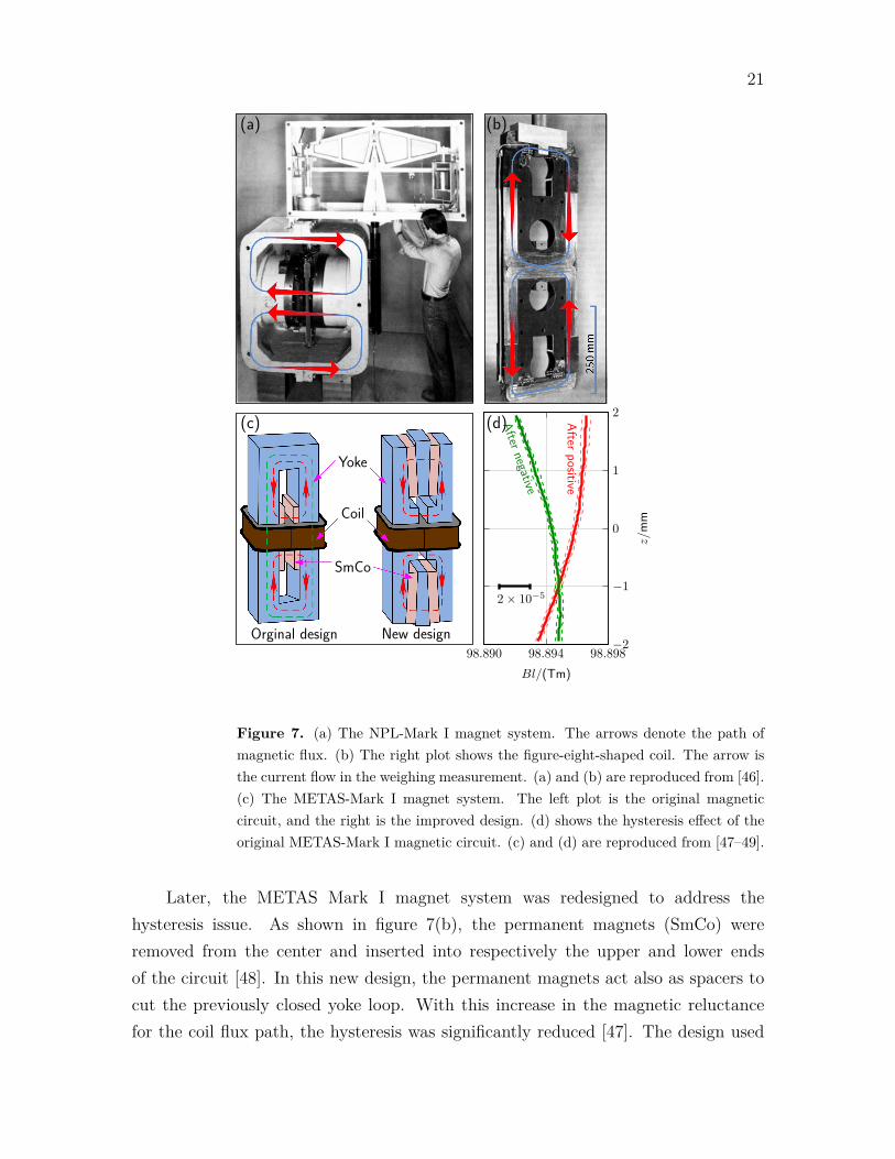
UK) [46]. The NPL-Mark I system is shown in figure 7(a) and (b). The constructionwas similar to an air-gapped transformer, but permanent magnet disks created theflux. The magnetic flux was guided horizontally through a 56 mm width, 0.3 m×0.3 msectional area air gap. The magnetic field in the air gap center was 0.68 T. A flatmagnetic profile was achieved with a figure-eight-shaped coil located vertically inthe center of the air gap. The total coil height was larger than the gap height,which ensured that in velocity mode, the magnetic flux through one half of the coilincreased while the other half decreased. With symmetry, the difference betweenupper and lower segments gave a linear change of magnetic flux over z.

The strong magnetic field in the NPL Mark I system was achieved by compressingthe flux in a relatively small measurement region. Almost no flux was wasted tothe outside of the measurement region. Therefore, the dissipation in the coil duringweighing was no longer a limiting factor for the measurement. The magnetic shielding,compared to coil systems, has been improved. The only downside of this design isthat only a tiny fraction of the wire length contributes to the force. The system wasmassive: the magnet weighs 6000 kg, and the coil 30 kg. A large mass can increase thethermal capacity and damp the effects of temperature. However, it is cumbersome toput such an extensive magnet system in a vacuum. Another disadvantage is that thefringe field goes through upper and lower coil segments. Hence, a large part of thefringe field is a common mode in the velocity and the force measurement. The firstgeneration Kibble balance experiment (METAS Mark I) at the Federal Institute ofMetrology (METAS, Switzerland) employed a magnetic circuit that is similar to theone in NPL’s Mark I. The original design is shown in the left plot of figure 7(c). Themagnetic circuit principle was the same as NPL Mark I, and a magnetic flux densityin the 7 mm width air gap, of about 0.5 T, was achieved [49]. The main differencewas that the ’8’ shape coil was arranged horizontally through the air gap. Note thatthis setup leaves a closed yoke loop shown as the green dashed line in figure 7(c).Ideally, with the same ampere-turns of two segments of the ’8’ shape movable coil,the total magnetic flux through the closed loop is zero. However, the asymmetryduring the weighing measurement, e.g., a non-synchronization of loading or removingthe coil current, can considerably shift the yoke BH status and introduce a magnetichysteresis during the mass-on and mass-off measurement loop. Figure 7(d) presentsa typical profile measurement after different current polarities [49]. It shows thehysteresis effect was at the order of 10−5, which became the major limitation forfurther improving the overall measurement accuracy.

21

98.890 98.894 98.898−2

−1

0

1

2

2× 10−5

After negative

Afterpositive

Bl/(Tm)

z/m

m

(a) (b)

(c) (d)

Orginal design New design

Yoke

Coil

SmCo

Figure 7. (a) The NPL-Mark I magnet system. The arrows denote the path ofmagnetic flux. (b) The right plot shows the figure-eight-shaped coil. The arrow isthe current flow in the weighing measurement. (a) and (b) are reproduced from [46].(c) The METAS-Mark I magnet system. The left plot is the original magneticcircuit, and the right is the improved design. (d) shows the hysteresis effect of theoriginal METAS-Mark I magnetic circuit. (c) and (d) are reproduced from [47–49].

Later, the METAS Mark I magnet system was redesigned to address thehysteresis issue. As shown in figure 7(b), the permanent magnets (SmCo) wereremoved from the center and inserted into respectively the upper and lower endsof the circuit [48]. In this new design, the permanent magnets act also as spacers tocut the previously closed yoke loop. With this increase in the magnetic reluctancefor the coil flux path, the hysteresis was significantly reduced [47]. The design used

22

for METAS Mark I succeeded in realizing a compact design using a one-dimensionhorizontal magnetic field. Still, the ’8’ shape coil suffers from a bad active-to-passivecoil ratio. Only ≈25% of the coil contributes to the Kibble principle, but all 100%contribute to the resistive loss in the weighing mode.

3.4. Radial permanent magnet system

As shown in Figure 8(a), the second generation Kibble balance at the NPL [50, 51],known as NPL Mark II, used a radial magnetic system and utilize all the wire inthe coil for the Kibble principle. In weighing mode, every piece of wire that hasdissipation also produces a force. The active-to-passive coil ratio is one. This designis the first with a cylindrical air gap. The NPL Mark II design has up-down symmetry,and soft yokes guide the magnetic flux of the permanent magnet ring (SmCo) throughthe upper and lower air gaps. The movable coil, split into two segments in oppositeconnection similar to the magnet shown in figure 5, uses the full wire length to producean electromagnetic force in the weighing and the induction in the velocity phase. Theradial field in the center part of each air gap is close to the 1/r field distribution,satisfying Olsen’s idea. The splitting of the coil significantly suppresses the commonnoise and produces a very quiet measurement in the velocity phase [6].

The shielding of the NPL Mark II system has been improved compared to theMark I system. But still, since the SmCo ring is located at the outer yoke and theair gaps contain open ends on the top/bottom surfaces. Flux leaks out at theselocations. After the Mark II apparatus was transferred to the National ResearchCouncil (NRC, Canada) in 2009, the NPL group started a new generation Kibblebalance experiment [15], referred to here as the NPL-NG system. The NPL-NGexperiment still uses the two-coil design with significant improvement on the magnetshielding: As shown in figure 8(b), the permanent magnet ring is located inside theinner yoke. Additional shielding has been considered for the NPL-NG design to cutthe coupling between the magnet flux and the external flux.

It is easy to imagine the NPL two-gap design with one gap closed. Closing onegap further compresses the magnetic flux, and yields an increased flux density inthe remaining gap. This idea has been implemented at the Laboratoire National deMetrologie et d’Essais (LNE, France). The LNE magnet is shown in figure 8(c). Witha 9 mm width air gap, an average field in the air gap of 0.95 T was obtained [32]. Thisfield strength is the strongest magnetic field used in Kibble balance experiments byfar. As a result of the broken up-down symmetry, the theoretical magnetic profile

23

×

×

×

×

×

×

×

(a) NPL-II type

(b) NPL-NG type

(c) LNE type

(d) BIPM type

(e) MSL type

Yoke SmCo magnet Air

−→M× Coil Flux path

Figure 8. Different radial permanent magnet systems for Kibble balances.

24

over z in the air gap will be sloped (shown in figure 12(d)) because the inner fluxpath has a lower reluctance compared to that of the far-end path. To correct it, fineadjustments, detailed in section 5, are required. ‘ As shown in figure 8(d), in 2006,researchers at the Bureau International des Poids et Mesures (BIPM) proposed a novelpermanent magnet circuit design that guides the magnetic flux of two permanentmagnets (SmCo) rings through one air gap [31]. Its construction is equivalent to thesymmetrical assembly of two LNE-type magnets with SmCo rings inserted in the inneryoke. This design has three advantages: 1) Soft yokes entirely surround the magnetcircuit, and therefore the magnetic shielding is nearly perfect [52]. Imperfections inthe shielding are created by holes that are required to connect to the coil. 2) Similarto the LNE design, since there is only one gap, the flux density in the gap is high andalmost no flux is wasted. 3) Since the geometry is symmetric about z = 0, so is theprofile. Hence at that vertical position, the radial field is proportional to 1/r. Dueto the symmetry, several systematic errors such as nonlinear magnetic effects [53,54]are reduced.

The attractive force at a horizontal plane where the magnet can be opened for coilinstallation can be very strong (kN level). Therefore in the BIPM magnet system, thecoil should be inserted before the circuit is closed. Accessing the coil is difficult afterthe magnetic circuit is closed, which may be inconvenient for in-situ coil adjustments.By far, the BIPM type magnet design is the most popular magnetic system appliedin worldwide Kibble balance experiments, e.g., [9, 11,13,14,33].

The Kibble balance experiment at the Measurement Standards Laboratory(MSL, New Zealand) employs a magnetic circuit as shown in figure 8(e) [12]. Thepermanent magnet is a cylinder with a radial magnetization inserted in the outer yokepole in the one-gap structure. This design can lower the coil flux coupling around theair gap [55]. However, similar to the original METAS Mark I design, a low reluctancepath exists along the yoke. The addition of two spacers in the inner yoke reduces themagnetic hysteresis. The spacers increase the magnetic reluctance for the main fluxpath and lower the magnetic field in the measurement gap.

In summary, yoke-based radial magnetic systems can produce a strong (sub-Tesla), robust and uniform magnetic fields for Kibble balance measurements. Inaddition to the high field quality, the magnet size is compact, and its operation cost,compared to the superconducting system, is low. Hence, the popularity of thesedesigns in current ongoing Kibble balances. Figure 9 compares the performance ofdifferent yoke-based radial systems, including the NIST-3 superconducting system.

25

Efficiency

ShieldingSymmetryBIPM

NPL-NG

MSL

NPL-II

LNE

Super

conduc

ting coi

l

Figure 9. Comparison of different radial magnetic systems along three dimensions:Symmetry, shielding, and efficiency.

Three features are compared: 1) the efficiency of creating the required magnetic field.2) the magnetic shielding. 3) the symmetry for Kibble balance measurement. Itcan be seen that the BIPM-type magnet system has good performances for all threefeatures. We believe the BIPM-type circuit is one of the best Kibble balance magneticsystems, and it will be taken as examples in most cases of the following discussions.

4. Design of a permanent magnet

In this section, we discuss the design of the magnet system in more detail. Theequations that were introduced in section 3 are now applied. We start by discussingthe material selection. Next, we will provide an example calculation of the magneticflux density in the gap. Then, we show how to calculate the working point of theyoke. After that, we will consider several ways to improve the flatness of the profile.In the subsection that follows that we provide a more detailed analysis of the forcethat is required to open the magnet and how to reduce this force. We will end thesection with an examination of the thermal properties of the magnet.

4.1. Selecting materials

The primary components of the air-gap type magnet are the active magnetic material(rare earth) and the yokes. For the active magnetic materials, the critical graph is

26

the demagnetization curve. That is the part of the B-H relationship, also calledthe hysteresis curve, in the second quadrant (negative H, positive B.) Figure 10(a)shows the demagnetization curves of several commercially available magnet materials.The rare-earth magnet materials have two unique features. (1) their demagnetizationcurves are almost straight lines. (2) they have a large maximum energy product(BH)max. The maximum energy product is the largest rectangle with sides parallelto B and H that can be found underneath the magnetization curve.

Since, at the percent level, the demagnetization curve for rare earth magnetmaterials can be considered linear, only two parameters are required to describe it.The magnetic flux produced by the magnet Bm as a function of Hm is given by

Bm = µmµ0(Hm −HC), (30)

where µm is the relative permeability of the material, and HC the coercivity, i.e.,the magnetic field required to drive the magnetic flux produced by the magnet to 0.For most of today’s magnet materials, µm ≈ 1. We use this approximation for allcalculations below.

A larger HC value will create a stronger flux density in the air gap in Kibblebalance magnetic circuits (details are discussed in 4.2). A large magnetic flux B

is desired for Kibble balance magnets according to the considerations in section 1.Hence, high HC materials, such as NdFeB and SmCo, are great candidates for themagnetic material for a Kibble balance magnet. To date, the highest possible HC

is achieved with sintered NdFeB magnets. Its HC is about 10 % larger than the HC

achieved with Sm2Co17, and, hence produces 10 % more magnet flux with the samevolume of the permanent magnet material. So, it seems NdFeB would be the bestmaterial to use in a Kibble balance. However, there is a second parameter that shouldbe considered, the temperature coefficient.

In general, the magnetic flux in the Kibble balance must be as stable as possiblefor environmental influences. One such influence is temperature. The sensitivityof the magnetic materials to temperature changes is expressed in the temperaturecoefficient of the magnetic material. It denotes the fractional change of the remanenceper one-kelvin change of temperature and is often abbreviated by α. For NdFeB,α ≈ −1 × 10−3/K and for Sm2Co17, α ≈ −3 × 10−4/K. Hence, the SmCo is aboutthree times more stable to temperature changes. Most designers prefer the smaller(in absolute, irrespective of the sign, terms, |α|) temperature coefficient of SmCo andaccept a 10% smaller remanence. This decision was made even harder with the recentdiscovery of (Gd,Sm)2Co17. There, Gadolinium (Gd) is alloyed with Samarium before

27

sintering it with Cobalt, and the result is a magnetic material with an even smallertemperature coefficient, α ≈ −1× 10−5/K. However, using (Gd,Sm)2Co17, instead ofSm2Co17, will reduce the magnetic flux by another 20 % [56,57].

A good proxy to quickly evaluate the temperature sensitivity of any magneticmaterial if the temperature coefficient is not readily available is the Curie temperature,Tc. At the Curie temperature, the magnet loses all its magnetization. The lower theCurie temperature, the higher the temperature coefficient. For SmCo, Tc = 825 °C,for NdFeB, Tc = 310 °C.

Another way to decrease the temperature coefficient of the complete magnetsystem is to use a shunt. This technique is described in the last part of this section.A lower temperature coefficient is achieved, but also the magnetic flux density at thecoil is smaller because some of the flux is diverted from the air gap through the shunt.

Having discussed the magnetic material, it is time to say a few things aboutthe second component in the magnet system, the yoke. The yoke aims to guidethe magnetic flux from the permanent magnet to the air gap and back. For thispurpose, the reluctance of the yoke has to be small according to equation (21). Thereluctance is Ry = ly/(µ0µrS). Hence besides a large cross-sectional area S and ashort magnetic path ly, a large relative permeability µr is desired. Including the smallreluctance, choosing a material with a large relative permeability has the followingthree advantages:

(i) It conducts more flux, and it increases the efficiency of the circuit.(ii) It is easier to engineer the profile in the gap, as the side walls made from high

µr are at more uniform potentials [59].(iii) It helps to reduce nonlinear magnetic errors [53,54], because the weighing current

influences the magnetic flux in the air gap to a lesser extent.

Note that although some sheet materials can have very high permeability, suchas µ-metal, steel sheet, they are typically not used in Kibble balance magnet systemsfor two reasons. First, the yoke needs to withstand a typical attraction force at the kNlevel [33]. Therefore solid material instead of sheet stock is preferred. Second, whilethe stack of sheets seems feasible, the tiny air gaps in the stack structure increase thereluctance of the yoke and decrease the uniformity of the flux in the air gap.

In practice, materials with relative permeabilities of 1000 or more are suitablefor yokes in Kibble balance magnets. Figure 10(b) and (c) reproduce the B-H curveand the permeability of three typical yoke materials, i.e., low-carbon steel, pure iron,and Fe-Ni alloy (50/50), which were used respectively in NIST-4, NIM-2, and BIPM

28

−1,000 −800 −600 −400 −200 00.0

0.5

1.0

1.5

NdFeB(sintere

d)

Sm2Co17

MF14SmCo5

NdFeB(isotrop

ic)

ceramic ferri

te

Alni

co

H/(kA m−1)

B/T

0.5

1.0

1.5

B/T

101 102 103102

103

104

105

H/(Am−1)

µr low-carbon steel

pure ironFe-Ni alloy

(a)

(b)

(c)

Figure 10. (a) Demagnetization curves for some commercially available rare earthmagnetic materials along with ferrites and AlNiCo. (b) B-H curve and (c) µr-Hcurve of three typical soft yoke materials. The low-carbon steel, pure iron, andFe-Ni alloy (50/50) are respectively used for building NIST-4, NIM-2, and BIPMmagnets [30,33,58].

29

systems [30, 33, 58]. It is recommended to heat-treat the parts after machining. Themachining process can lower the permeability, and heat treatment can reverse theloss in permeability [33,58].

4.2. Magnetic flux density in the air gap

In the following paragraphs, we calculate B in the gap using the BIPM type magnetas an example. Other magnetic circuits can be analyzed similarly.

The first step in the design process is to find the dependence of the magneticflux density in the air gap on the dimensions of the system. The symmetry of themagnet system can simplify this process. The number of green flux paths in figure8 shows the symmetry of the system. For the BIPM type magnet, only a quarter ofthe complete circuit needs to be analyzed as indicated in figure 11(a) and (b). Aswe show in section 2.3, the easiest way to analyze this circuit is to convert it intoan equivalent electrical circuit. The permanent ring is providing the MMF (similarto the voltage source), and the reluctance (resistance in an electrical circuit) of threecomponents, i.e., the permanent magnet, the yoke, and the air gap, is written as

Rm =δm

µmµ0Sm

, Ry =δy

µyµ0Sy

, Ra =δa

µ0Sa

, (31)

where δm, δy, δa denote the length; Sm, Sy and Sa the cross-sectional areas; and µm,µy, and µ0 the relative permeabilities of the permanent magnet, the yoke and the airgap. For now, we assume the flux completely penetrates the air gap, ignoring fringefields at the upper and lower end of the air gap. It is shown in section 2.3 that apermanent ring can be seen as a battery with MMF F = −HCδm while leaving thespace as vacuum (air), i.e. µm ≈ 1. The three reluctances form a series connection,hence by Ohm’s law,

(Rm +Ry +Ra)φ = −HCδm. (32)

For a high permeability yoke, Ry << Ra, Rm. Without loss in generality, we setRy = 0. The total flux through the air gap and the magnet is the same and can bewritten as the product of the cross-sectional area and the flux density, i.e.,

φ = SmBm = BaSa. (33)

Substituting equations (31) and (33) into (32), the magnetic flux density in theair gap can be solved [23]. It is

Ba =−HC

Sa

Sm

1

µmµ0

+δa

δm

1

µ0

30

r

z

δm

δa

A

BC

Rm

Ra

F

Ry

ϕRtCoil

Sm2Co17 magnet

Sm2Co17 magnet

N

S

N

S

Yoke(a) (b) (c)

Figure 11. (a) shows the 3D construction of a BIPM-type magnetic circuit. (b)The analysis unit for the BIPM-type magnet. (c) The equivalent electrical circuit.The green and dashed green curves denote different main flux paths. The red lettersA, B, and C indicate cut-planes at three different locations, see text.

≈ −µ0HC

Sa

Sm

+δa

δm

≈ 1 T

Sa

Sm

+δa

δm

. (34)

Note that the last result is for Sm2Co17 magnets, for which µ0HC ≈ −1 T [33].It can be seen the air gap magnetic field strength Ba is determined mainly by tworatios, Sa/Sm and δa/δm. As mentioned above, the fringe fields at the edge of theair gap have been neglected. It can be taken into account by multiplying Sa with ageometrical factor γ > 1. This mathematical trick pretends that the air gap is tallerthan it actually is. More on this topic and how to reduce the fringe field can be foundin section 4.4.1.

4.3. Magnetic working point of the yoke

Two conditions are desired for the yoke. First, the yoke should not be saturated atany point. Second, the average yoke permeability should be high.

One can investigate the first condition by examining the cross-sectional area ofthe yoke along the flux path. In figure 11(b), three sectional planes are indicated bythe letters A, B, and C. The cross-sectional areas are SA, SB, and SC, respectively.Since flux is conserved the flux density in one area, here for example in region B, isgiven by

BB = BaSa

SB

. (35)

The area SB needs to be large enough to keep the BB below saturation in the yoke’s

31

B-H curve. The size and the weight of the magnet can be kept small by settingSA = SB [60]. SC is determined by dimensions of the permanent magnet and the airgap, and for most cases, SC > SA, SB to obtain enough coil movement range with auniform field distribution.

Maintaining a large average permeability in the yoke is important for threereasons. (1) To keep the MMF drop over the yoke small, delivering more fluxto the air gap, (2) to minimize nonlinear errors that occur when the coil carriescurrent [53, 54, 58] and (3) to achieve a flat field profile. A high yoke permeabilitymakes the two sides of the air gap equipotential surfaces, and the flux transversesuniformly through the gap. Yoke materials, such as the Fe-Ni whose B-H curveis shown in figure 10, have very high permeabilities so that all three points can beachieved.

4.4. Profile flatness

The phrase “flatness of the field” or ”flatness of the magnetic profile” includes tworelated goals. (1) the radial component of the magnetic flux density Br should beconstant with the traveling range of the coil along z. (2) the radial component ofthe flux density multiplied by the radius, rBr should be constant along r. The firstproperty ensures that the Bl is independent of the exact weighing position along z,see 3.1. With the second property, Bl becomes independent of the coil radius and,hence, of the coil’s thermal expansion during weighing.

Maxwell’s equation link the the two components of the flux density together via,1

r

∂(rBr)

∂r+∂Bz

∂z= 0, (36)

∂Br

∂z− ∂Bz

∂r= 0. (37)

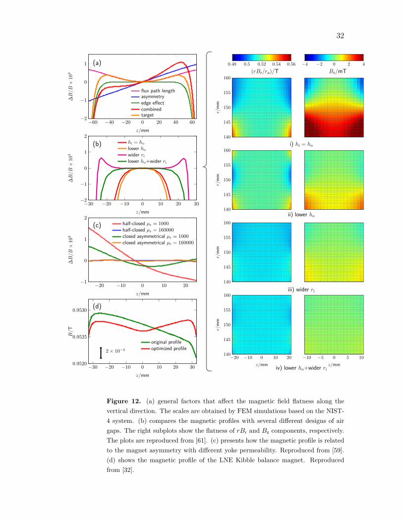
If Bz were constant, the two properties for a flat field would be met. However, thisperfection cannot be achieved over the entirety of the gap. Thinking about thisproperty reveals three sources of deviation from field flatness. (1) the fringe field atthe end of the gap (edge effect), (2) magnet asymmetry, and (3) the flux path length.All three effects are summarized in figure 12 (a).

4.4.1. Reducing the fringe field The field inside the gap depends on the aspect ratioof the gap. A narrow and tall air gap has a much more uniform field than a wide andshort air gap. This effect is analog to a similar problem in electrostatics, the field in aparallel plate capacitor. At the end of the air gaps, the flux lines bulge outward. Per

32

140

145

150

155

160

r/m

m

0.48 0.5 0.52 0.54 0.56 −4 −2 0 2 4

140

145

150

155

160

r/m

m

140

145

150

155

160r/

mm

−20 −10 0 10 20140

145

150

155

160

z/mm

r/m

m

−10 −5 0 5 10

z/mm

−60 −40 −20 0 20 40 60−2

−1

0

1

z/mm

∆B/B

×10

3

flux path lengthasymmetryedge effectcombinedtarget

−30 −20 −10 0 10 20 30−2

−1

0

1

2

z/mm

∆B/B

×10

3

hi = ho

lower ho

wider rilower ho+wider ri

−20 −10 0 10 20−1

0

1

2

z/mm

∆B/B

×10

3

half-closed µr = 1000

half-closed µr = 160000closed asymmetrical µr = 1000closed asymmetrical µr = 160000

−30 −20 −10 0 10 20 300.9520

0.9525

0.9530

2× 10−4

z/mm

B/T

original profileoptimized profile

(a)

(b)

(c)

(d)

(rBr/ra)/T Bz/mT

i) hi = ho

ii) lower ho

iii) wider ri

iv) lower ho+wider ri

Figure 12. (a) general factors that affect the magnetic field flatness along thevertical direction. The scales are obtained by FEM simulations based on the NIST-4 system. (b) compares the magnetic profiles with several different designs of airgaps. The right subplots show the flatness of rBr and Bz components, respectively.The plots are reproduced from [61]. (c) presents how the magnetic profile is relatedto the magnet asymmetry with different yoke permeability. Reproduced from [59].(d) shows the magnetic profile of the LNE Kibble balance magnet. Reproducedfrom [32].

33

unit area, the yoke near the end of the air gaps carries less flux than in the center ofthe gap. In other words, the reluctance near the air gap end is larger, and hence themagnetic flux density is smaller. The edge effect can easily lead to a magnetic fieldreduction at the percentage level. With the edge effect, the region where the fieldis uniform, e.g., ∆B/B < 5 × 10−4, can be significantly smaller. As a result, a flatprofile can only be obtained near the center of the magnet, and only about 50% ofthe gap may be usable [33, 59]. For a gap with parallel sides of equal height, ha, [61]gives an equation for the relative deviation of the radial magnetic flux as a functionof vertical position. It is,

Br(z)

Br(0)− 1 = − exp

[−(

1 +π(ha − 2|z|)

δa

)]+ exp

[−(

1 +πha

δa

)], (38)

where ha and δa denote the air gap height and width, respectively.In a BIPM-type magnet, the yoke-air boundary at the end of the air gap,

however, is not symmetric even when the heights of inner and outer yokes areequal (hi = ho) [62]. The difference is noticeable: the inner boundary containsthe permanent ring and the yoke, while the outer yoke has only yoke material. Asa result, the magnetic flux lines at the gap end will slope further towards the outeryoke. Because of this, magnetically, the outer yoke is higher than the inner yoke, evenwhen they are geometrically the same. The red line in figure 12(b) and the right topplot i) present the Br and Bz distribution in the central region of the air gap withhi = ho. Large Bz gradients are seen in both r and z directions, and therefore theprofile quality in this case (hi = ho) is not high.

So far, we tacitly assumed that the air gap is bounded by vertically aligned ironpieces of the same height. In other words, the air gap has perfect symmetry. However,as described above, the MMF is not symmetrically placed to the air gap. The sourceof the magnetic field is closer to the inner yoke. Hence, the path to the outer yokehas more reluctance, and the symmetry is broken. As a consequence, the flux linesbend towards the outer yoke. It appears that the magnetic height of the outer yokeis higher than the physical height. This phenomenon can be remedied in two ways.First, the symmetry can be restored by adding additional magnetic material on theoutside yoke [62]. Second, the magnetic symmetry can be restored by lowering theouter yoke such that magnetically the two sides of the air gap have identical heights.This idea is described in [63].

The effect of changing the outer yoke height is illustrated in figure 12. On the

34

right side of the figure, the magnetic flux in the air gap is shown. The top rowshows it for the case where both heights are identical. The second row shows it forho < hi. Lowering the outer yoke improves Bz. The top right surface plot in thefigure shows all shades from dark red to blue, where the plot one row below onlyshows the colors in the middle of the range. Disappointingly, the radial field is notmuch improved. This point is also illustrated in panel (b) of figure 12. The orangeline shows Br(z)−Br(0) as a function of z. The orange line is calculated for ho < hi

and the red line ho = hi. There is a small but not significant gain in uniformity forho < hi compared to ho = hi. A similar (small) effect can be achieved by addinga pair of SmCo magnets to the outer yoke. However, doing so will compromise theshielding property of the yoke. Fluctuating external fields will be able to reach thecoil.

Reference [61] proposes another technical solution to improve field flatness:Adding a piece of iron rings with a rectangular cross-section at the upper and loweredges of the gap. These features decrease the gap size at the end of the gap, effectivelyreducing the reluctance and increasing the flux. The flatness of Br(z) can be optimizedby adjusting the two parameters of the rectangle, the height, and the width of therectangle. An example (parameters were shown in [61]) is shown in the third rightsubplot iii) and magenta curve in figure 12(b). It can be seen in this case the1/r field distribution for Br(r) has better quality than is achieved by lowering ho.More important, the usable measurement range for Br(z) has been greatly increasedcompared to the original design (hi = ho). As shown in subplot iv) and the greencurve in figure 12(b), a flatter field distribution of rBr and Bz can be obtained if bothtechniques of lowering ho and widening ri are applied.

4.4.2. Improving magnet symmetry The second factor that can significantly improvefield flatness is, in general, the overall symmetry, and more specifically, the up-downsymmetry of the magnet system. By design, the BIPM type magnet system exhibitsperfect mirror symmetry around z = 0. However, this symmetry can be broken dueto machining tolerances, assembly, and material inhomogeneities. Concrete examplesthat break the symmetries are

• The gap could be slightly tapered due to machining tolerances.

• Dowel pins or bolts used to align and fasten components of the magnet systemcould introduce magnetic asymmetries.

• The magnetization of the upper SmCo ring could be different from the lower

35

ring.

• The permeability of the iron could be inhomogeneous.

The latter is especially troublesome because the permeability depends not only on thestresses induced during fabrication but also on the magnetic history. For example,during the construction of NIST-4, it was discovered that the procedure used to closethe magnet had an effect on the permeability of the yoke and changed the profileflatness [33].

Materials with high permeability ease some of these problems. Ideally, the twosides of the gap are equipotential surfaces. So the MMF-drop is the same betweenany points on each side of the gap. Materials with a high µr, such as Fe-Ni (50/50)alloy, can be used to achieve the equipotential surface. An impressive illustration ofthe power of high µr materials is the BIPM magnet [59]. The top cover of the BIPMmagnet is missing, but the field is reasonably flat. This fact is demonstrated in panel(c) of figure 12. These four curves are compared. The curves are obtained with anFEA calculation. The magnet is either half-open or complete. When the magnet iscomplete, the bottom SmCo disk has 10% more magnetization than the top disk. Foreach case, the field was calculated for µr = 1000 (soft iron) or µr = 160000 (50%Fe-50%Ni). For the latter case, there is no difference if the magnet is open or closed.This graph impressively demonstrates how a lack of symmetry can be overcome witha high permeable material. It recovers a perfect field even with half the flux pathmissing or, in the other case, with a 10% difference in magnetization.

In summary, we would advise the designer to start with a symmetric plan andbuild the yoke with high permeable materials if the construction budget allows thesematerials. The use of these more expensive materials can compensate for unwanteddeviations in the production process.

4.4.3. Equalizing the flux paths The third factor that has an influence on the shapeof the magnetic profile is the length of the flux path. The length of the flux pathchanges the profile, independent of the presence of a fringe field at the end of thegap. As shown in figure 11, the reluctance along the solid green line is greater thanthat of the dashed green line, and hence, the magnetic field in the gap center, Br(z),distributes as an ’M’ shape. The Br is lower at the center of the gap and then increasesbefore it rolls off to the end of the gap.

The length of the flux path is a powerful but yet simple argument, and it canguide our intuition for the pot magnet system employed by LNE [32]. The field at

36

the top of the gap has to be smaller because of the larger reluctance in the flux pathnecessary to reach the top. The reluctance increase can be counteracted by makingthe gap smaller by introducing a taper. The Br of a parallel and tapered gap of theLNE magnet is shown in panel (d) in figure 12. The taper runs from the center ofthe gap to the top. The gap with a nominal width of 9 mm is 8 µm smaller at thetop. The yoke material used here does not have an exceptionally high µr.

In summary, visualizing the length of the flux path in the magnet is a valuabletool to get a qualitative understanding of the profile in the magnet. Differences in fluxpaths can be compensated by adjusting the gap size. The effect that different lengthflux paths have on the profile is more pronounced if the permeability of the yoke islow. So, these differences can be evened out by using high permeable materials.

4.5. Force required to open the magnet

Magnet systems that entirely enclose the coil apart from a few holes to attach the coilare called closed yokes. These designs have superior shielding performance comparedto the open-yoke designs. However, the yoke needs to be opened and closed at leastonce to install the coil. The force required to open the magnet can be large, on theorder of several kN. Therefore, a dedicated device called a magnet splitter is requiredto open and close the magnet system in a controlled way. The magnet splitter, suchas the one used for NIST-4 [33] can only be used when the magnet is not installedin the balance. It is difficult to integrate such a device into the balance for in-situadjustments.

Here we follow the Maxwell stress tensor method and the derivation given inthe appendix of [57] and show how to reduce the splitting force as much as possible.It is assumed that the split plane is horizontal, and, hence, dS is vertical. In thiscase, only the last row of T is relevant. As it is shown in figure 13, the vertical forcesimplifies to,

Fz(z) =πraB

2

µ0

(δa −

2πra(Si + So)

SiSo

z2

), (39)

where ra = (ri + ro)/2 is the mean radius of the air gap, B the average magnetic fluxdensity in the air gap, So, Si the cross-sectional area of the outer and inner yokesat the splitting plane, and Bo, Bi the magnetic flux density at these surfaces. Thedistance of the split plane to the symmetry plane of the magnet is denoted by z.

The force calculated with equation (39) occurs at the initial separation, at themoment when the contact between the metal surfaces breaks, i.e, d = 0. This force

37

δa

PM

PM

Inner yoke

Oute

ryok

e

B

Bzi

Bzo

Si So

z

zr

Figure 13. Schematic integration of the Maxwell stress tensor to determine theforce required to split the magnet. The symmetry plane is given by the horizontaldashed line. The split plane is a distance z away from the split plane.

can be made zero by choosing

|z| = z0 :=

√δaSiSo

2πra(Si + So). (40)

With increasing |z|, the direction of the force changes. For |z| < z0, Fz(d = 0, z) isrepulsive and for |z| > z0, it is attractive.

Equation (39) gives and analytical expressions for the force required to openthe magnet [57]. In reality, however, the magnetic force changes as the gap opens,because Bzi, Bzo and B are functions of the yoke separation d. In order to insert thecoil into the magnet, a separation greater than the coil height, i.e. d > hc is required.Therefore, the magnetic force Fz should also contain the dependence on d. Here wetake the NIST-4 magnet system as an example. By finite element analysis (FEA), thedistribution magnetic force Fz as a function of the two parameters z ∈ (−80, 80) mmand d ∈ (0, 20) mm is shown in figure 14. At the start of the separation, d = 0, theforce calculated by FEA agrees with (39), see the cyan curve in the right subplot. Inred, this subplot also contains a calculation of Fz for d = 20mm. It can be seen thatthe latter curve has a similar behavior to the one at d = 0, but is much flatter.

38

0 4

force/kN

Fz,d=0mm

Fz,d=20mm

Max(Fz)Min(Fz)

4

3

2

2

1

1

0

0

−1

−1

−2

−2

−3

−3

−4

−4

−5

−5

−8

−8

−10

−10

−15

−15

0 5 10 15 20

−75

−50

−25

0

25

50

75

Separation distance d/mm

Split

ting

plan

ez/m

m

0

2

4

Fz/k

N

z = ±35.5mmz = ±25mm

Figure 14. The main plot shows the splitting force Fz as a function of twoparameters, the position of the splitting surface z and the separation between theyoked d. The unit of the force is kN. A positive (negative) force means the twoparts of the magnet repel (attract) each other. For this magnet, the precision gap isbetween −50 mm and 50 mm. The right plot presents the magnetic force Fz alongtwo vertical lines at d = 0 mm and d = 20 mm, as well as the force boundaries(maximum and minimum values of Fz) required to open the magnet within 20 mmat different splitting planes. The top subplot shows the magnetic force as a functionof the separation distance d at the two locations, z = ±25 mm and z = ±35.5 mm.

39

For the construction of the splitter, it is necessary to know how much the forcechanges during the splitting process. The yellow shaded area in the right subplotof figure 14 indicates the dynamic range of the force. For a given z the yellowshading extends from the Fz,min to Fz,max. The reader can identify three regions.For |z| > 68.5 mm, both extreme forces are negative. Hence, during the splittingprocess, there will always be an attractive force between the two parts of the magnet.For |z| < 35.5 mm, the splitting force is repulsive for all d. For all other z values, thesplitting force changes sign. It is attractive at first when the magnet opens (d = 0)and becomes repulsive with increasing d. Such a load change is important to take intoaccount when designing the splitter. Interestingly, with the split plane at z ≈ 25 mm,the force stays fairly constant for the entire opening process.

The forces required to split the magnet (several kN) are about the same orderof magnitude as the weight of the whole or at least part of the magnet (g timesseveral 100 kg). The weight of one of the two parts that the magnet is split into,can be used to reduce the force that the splitter must generate. For example,the total mass of the NIST-4 magnet is 850 kg. If the splitting is performed atz = 25 mm, the weight of the upper piece is ≈ 3.3 kN and that of the lower ≈5.2 kN. Conceivably, one could use the 3.3 kN to work against the repulsive forceand reduce the maximum Fz(d = 5 mm, z = 25 mm) = 2.57 kN and the minimumFz(d = 0 mm, z = 25 mm) = 2.03 kN to combined downward forces of 0.73 kN and1.27 kN, respectively. Note, this is not what researchers at NIST are doing. Thesplit plane was chosen at z = −50 mm to be outside of the precision gap, and theheavier two-thirds of the magnet is lifted off. The theoretical Fz at z = −50 mm hasa minimum value of 4 kN. Adding the weight of the top piece, the maximum splittingforce required is 9.2 kN. The example should show, however, that by clever selectionof the location of the split plane and use of the weight, the split force can be wellminimized. A force at 1 kN level is achievable with lead screws. Therefore, it seemspossible that such a system can be integrated into the Kibble balance. Then, thesplitting and maintenance of the coil could be made in situ. One significant advantagewould be that the Kibble balance can be used to measure the profile, and one doesnot need to have a dedicated profile measurement system for fine adjustments of theprofile.

Note, the smallest splitting force, including the weight, occurs at z = ±25 mm,but the precision gap extends from −50 mm to 50 mm. If the split plane is located atone of these locations, the magnetic field profile near the break is disturbed. Hence,

40

the magnetic flux will only be smooth in a length of 75 mm. Placing the break in themagnet is a trade-off. As can be seen in figure 14, the smallest splitting force occursin or near the region of the precision gap. However, that is the location where thelocation of the split plane is least desirable.

4.6. Thermal considerations

The magnetization of the SmCo material has a temperature coefficient of about−3×10−4/K. Although the magnetic field drift is very smooth due to a large thermalcapacity and can be removed by ABA [64] measurement in Kibble balance, it ispreferred to reduce the temperature coefficient to a smaller level. While this step isoptional for SmCo, it is mandatory for NdFeB because its temperature coefficient ismuch higher.

Besides potentially adding a systematic bias to the measurement, a largetemperature coefficient has another significant downside. At pump down, mostsurfaces cool down due to the evaporation of a thin water film. Since the magnet’sthermal mass is large and is well insulated in a vacuum, it takes weeks for the magnetto equilibrate fully thermally. Thus, if the temperature coefficient of the magneticmaterial is significant, the measurement will drift for a long time. The drift addsuncertainty to the measurement, makes the investigation of systematic effects difficult,and is commonly not desired.

In general, there are two avenues to reduce the temperature coefficient ofthe magnet. First, one can choose an active magnetic material with a very lowtemperature coefficient, for example, (Sm,Gd)Co [9, 57], see section 4.1. Second, themagnetic circuit can be designed to be less sensitive to temperature. The latter ideais illustrated by the blue rectangle in figure 11. Part of the magnetic flux is routedthrough a shunt whose reluctance varies with temperature. Given the temperaturedependence of its reluctance, the geometry of the shunt can be finely tuned suchthat the flux in the air gap is relatively independent of temperature at the designtemperature.

As is shown in the equivalent circuit in 11, an additional reluctance, the shunt, isparallel to the permanent magnet. A small amount of magnetic flux φ′ goes throughthe shunt with reluctance Rt. The circuit, now, has two loops. One is carrying themain flux φ, the other the shunted flux φ′. Using Kirchhoff’s laws, one obtains,

(φ+ φ′)Rm + φ(Ra +Ry) = F (41)

(φ+ φ′)Rm + φ′Rt = F . (42)

41

Eliminating φ′ in equation (42) and ignoring Ry yields

φ ≈ F

Rm +Ra +RmRa

Rt

. (43)

To keep φ insensitive to temperature T , i.e. ∂φ/∂T = 0, equation (43) is written as1

F

∂F

∂T= − 1

Rm +Ra

RmRa

R2t

∂Rt

∂T,[

1

F

∂F

∂T

]= − RmRa

(Rm +Ra)Rt

[1

Rt

∂Rt

∂T

]. (44)

The expressions in square brackets denote the relative temperature coefficient of theMMF and the shunt reluctance. Temperature compensation with a shunt is possiblebecause the relative temperature coefficient of the MMF is negative, but that of theshunt is positive, typically a few percent per kelvin. Hence, Rt can be chosen suchthat equation (44) is valid. In that case, the temperature dependence of the flux inthe gap vanishes.

5. Delivering design to reality

Once the magnet has been designed, it’s time to build it. Once it’s made, it must beverified. The engineers and scientists have to determine the field and the flatness ofthe profile. Perhaps the magnet must be split open to insert the coil. The shieldingproperties of the magnet system must be measured, and finally, the temperaturecoefficient of the complete system must be determined. This section explains allthese tasks in detail. So far, we have dealt with an ideal magnet. Here, reality setsin.

5.1. Mechanical assembly and alignment

Ideally, on the horizontal plane xy at z = 0, the magnetic flux density should beuniform in the azimuthal direction and be proportional to 1/r in the radial direction.A deviation from these two desired goals could be caused by a nonuniformity ofthe magnetic materials, machining defects, misalignment during assembly, and otherproblems that break the symmetry. Although a slightly different coil placing canminimize these effects (see below), the best is to use good design to avoid theseproblems from the start with the following three tips:

(i) Use symmetric magnet rings. If two rings are employed, they should be asidentical as possible in size and magnetization. Very often, these rings are much

42

larger than the size that can be reasonably magnetized. In this case, each ring willbe composed of smaller segments that can be magnetized. It’s best to measureeach segment and assemble each ring such that the average magnetization isidentical. Also, scramble the segments in each ring so that azimuthal uniformityis achieved as best as possible.

(ii) Use high permeability yokes. High yoke permeability helps create equal potentialboundaries and, therefore, can largely average out the asymmetry. As themachining process could significantly lower the yoke permeability, heat treatmentbefore assembly is necessary.

(iii) Keep the assembly as symmetrical as possible. The magnetic working point onany material depends on its magnetic history. During the assembly, two yokepieces touch at one point instead of evenly around the circumference. The fluxthat flows through the point of contact can be very high, altering the magneticworking point at that spot. With the altered magnetic working point, thereluctance of the section has been changed, and the azimuthal symmetry of themagnet system is broken. Hence, try to assemble the pieces that carry magneticflux in an even, symmetric, and controlled fashion.

Next, we discuss how the geometric factor depends on the mechanical assemblyand how it is affected by the coil alignment. The magnetic flux density in the air gap,Br, is determined by the width of the gap. As we will see below, asymmetries canbe compensated by placing the coil eccentrically in the gap. However, the amountof eccentricity for the coil placement is limited since the coil should not touch theyoke. Therefore, this argument gives an upper bound on how much asymmetry can beallowed. For now, the inner and outer yokes are assumed to be perfect cylinders. Inthis case, misalignment can occur when (a) the cylinder axes are not parallel with oneanother, or (b) if the cylinder axes are not coincident at z = 0 and (c) a combinationof (a) and (b). All three cases will cause an azimuthal variation of Br. In a perfectsymmetrical magnet, Br is independent of the azimuth, i.e., ∂Br/∂ϕ = 0. Let’sassume that this assumption is no longer true. An example where the inner yoke isdisplaced along the negative x axis is shown in Fig. 15(a). Since the gap is smallestalong the positive x axis, the force is largest. The force on a coil carrying current isindicated by the black vectors and the red curve connecting the tips of the vectors.The force is no longer isotropic but is larger at ϕ = 0 and smaller at ϕ = 180.Interestingly, the total Bl along the whole coil is conserved, as is shown in [37]. Thisis because, to first order, the reluctance of the gap does not change by displacing the

43

inner yoke and hence the flux through the coil and with that the flux gradient or Bl(see Appendix A) remains the same.

If one were to plot the vertical force Fz as a function of azimuthal angle ϕ, onewould obtain a cosine shifted by an offset. The maximum would occur at 0 andthe minimum at 180. This relationship can be visualized by a polar plot, as shownin Fig. 15 (c). The force on the right side of the coil is larger than on the left.Hence, a torque τy about the y axis occurs. Correspondingly, in velocity mode, aninduced EMF can arise if the coil rotates around y while sweeping vertically [35].This additional EMF can lead to a bias in the measurement.

There is an easy way to avoid the bias in velocity mode and eliminate τy: Placethe coil eccentric to the coordinate center. The amount the coil needs to be moved is

∆r =∆Br

2Br

rc, (45)

where Br is the average radial magnetic flux density at the coil and ∆Br is thedifference between the maximum and the minimum of Br. The coil has to be movedtoward the maximum field. So, in the above example, in the direction of +x. Notean analytic equation for ∆Br based on the eccentricity of the inner yoke can be foundin [37].

The gap width is given by the difference in radius of the outer and inner yoke,δa = ro− ri. By subtracting the width of the coil from δ the air space around the coilis obtained. If the coil is centered, which is usually the case, half of the air space isinside and the other half outside of the coil. The maximum distance the coil can bemoved is given by

∆r <δa − wc

2(46)

Hence, the maximum relative asymmetry that can be cancelled with this techniqueis given by

∆Br

Br

<δa − wc

rc

(47)

The second coil misalignment discussed here is a tilt. One can tilt the coil toreduce the angle between the coil and the magnetic field plane so that the horizontalmotion of the coil is minimum. As shown in figure 15 (d), when the coil is tilted withrespect to the Br field, a horizontal force is generated due to the vertical current.Here, we assume the Br to be horizontal. The distribution of the horizontal forcecomponent along the wire circular is shown in figure 15(f). To fix this, it requires totilt the coil to where the coil displacement (proportional to horizontal force) is zero

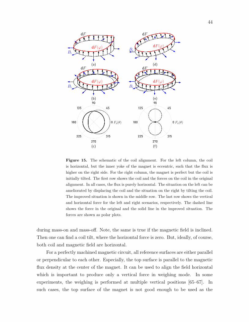
44

Br

Br

Br

Br

dF

dF

dF

dF

dF (φ)

dF (φ)

dF (φ)

dF (φ)

Fz(θ) Fx(θ)

(a)

(b)

(c)

(d)

(e)

(f)

Figure 15. The schematic of the coil alignment. For the left column, the coilis horizontal, but the inner yoke of the magnet is eccentric, such that the flux ishigher on the right side. For the right column, the magnet is perfect but the coil isinitially tilted. The first row shows the coil and the forces on the coil in the originalalignment. In all cases, the flux is purely horizontal. The situation on the left can beameliorated by displacing the coil and the situation on the right by tilting the coil.The improved situation is shown in the middle row. The last row shows the verticaland horizontal force for the left and right scenarios, respectively. The dashed lineshows the force in the original and the solid line in the improved situation. Theforces are shown as polar plots.

during mass-on and mass-off. Note, the same is true if the magnetic field is inclined.Then one can find a coil tilt, where the horizontal force is zero. But, ideally, of course,both coil and magnetic field are horizontal.

For a perfectly machined magnetic circuit, all reference surfaces are either parallelor perpendicular to each other. Especially, the top surface is parallel to the magneticflux density at the center of the magnet. It can be used to align the field horizontalwhich is important to produce only a vertical force in weighing mode. In someexperiments, the weighing is performed at multiple vertical positions [65–67]. Insuch cases, the top surface of the magnet is not good enough to be used as the

45

field reference. Reference [63] gives a practical and elegant way to measure thefield inclination. A rotating magnetometer that is instrumented with capacitiveprobes is lowered into the gap at different positions. At each position, the probeis centered in the gap using the signal of the capacitive probes. From the readingof the magnetometer, the tilt of the magnetic field can be obtained. Finally, theexperimenter has to be aware that changing the tilt of the magnet will also requirechanging the position of the coil if one wants to generate a purely vertical force inthe weighing mode, see (46). Hence, one has to be aware of the available parameterspace. Is it possible to tilt the magnet by the desired angle without the coil touchingthe yoke? Only if the answer is in the affirmative, does it make sense to carry on withthe experiment.

5.2. Profile measurements

After the magnet is assembled, it is advisable to measure the flatness of the profilebefore integrating the system into the experiment. In this way, it is much easier totweak the magnetic profile, i.e., shim the magnet, should it become necessary.

There are two principal ways one can measure the profile of the magnetic fluxdensity. The measurement can be performed at selected points with a probe, oran integrated flux (Bl) can be measured with a coil. The information provided bythe latter measurement is more applicable to the Kibble balance experiment. Themeasurement at discrete points is often easier to carry out and does not requirededicated hardware.

Using a probe, one must be aware that the field gradient along r direction is large,and thus the probe measurement requires a perfect vertical motion relative to the yokesurface. For example, the field gradient of the NIST-4 system is ∆B/B = −∆r/rc,and for a ∆B/B resolution of 1×10−4, the probe variation along the r direction, ∆r,should be less than 10−4 · rc = 21.5 µm.

Unlike a probe that can be used to spot-check the profile, a coil can be used to getan integrated result along a path. Similar to the Kibble balance experiment, voltagesU and velocities v are measured along the trajectory. However, since the measurementis performed before the magnet is integrated into the balance, an auxiliary device mustbe used to move the coil. As a result, the velocity cannot be measured precisely andmay not be constant along the trajectory. Furthermore, the measurement is oftennoisy due to vibrations. The noise is further exacerbated by the fact that the velocityand voltage measurements are typically and, unlike in a Kibble balance measurement,

46

0.66

0.68

0.70

0.72

U/V

−0.1

0.0

0.1

∆U

/V

−60 −40 −20 0 20 40 60

−50

0

50

z/mm

∆B/B

×10

3

(a)

(b)

(c)

Figure 16. An example of measurement result obtained with the gradiometer coil.(a) shows the absolute induced voltage and (b) is the differential signal of upperand lower coils. (c) compares the magnetic profiles represented by the single coilmeasurement and the gradiometer coil measurement.

not perfectly synchronized. Hence, vibrations do not cancel when the quotient U/v iscalculated. This is illustrated by the green curves shown in figure 16 (a) and (c). Thedata in this figure are from actual data measured at NIST [33]. The peak-peak valueof ∆B/B is over 5× 10−2, and even with careful averaging, it is difficult to measurea change in the magnetic flux density with relative uncertainties below 1× 10−3.

Reference [33] provides an excellent solution to overcome these measurementchallenges. The idea is to use a gradiometer coil to detect the field variation insmall ranges. Then, a detailed profile can be obtained by merging the field gradientinformation with an averaged absolute profile determination (deduced from U/v

measurement). A gradiometer coil contains coils with the same parameters (number

47

of turns, average radius) separated by a vertical distance ∆z. In the measurement,the induced voltages in one of the two coils, U , and their differential output ∆U aremeasured simultaneously. Note that it is easier to measure voltages simultaneouslythan to measure voltage and velocity at the same time. The ratio of two signals canbe written as

∆U

U=Br(z)−Br(z −∆z)

Br(z)≈ ∆z

Br(z)

∂Br

∂z. (48)

Using Br(z) = U/(2πrcNv), the magnetic profile Br(z) can be solved by numericallyintegrating equation (48) along the measurement interval, i.e.,

Br(z) =1

2πrcNv∆z

∫ z

zstart

∆U(z′)dz′ +O, (49)

where the constant O is a chosen such that Br(0) = U/(2πrcNv). Figure 16 (b)shows the differential voltage ∆U in the same example, and (c) compares the magneticprofiles obtained by U/v measurement and the gradiometer coil determination. It canbe seen that the signal-to-noise ratio has been improved by three orders of magnitudeby the simple gradiometer coil.

It is also possible to build a radial gradiometer coil. Here two coils are placedradially separated. The researchers may use a radial gradiometer coil to check the1/r dependence of the magnetic flux density [33].

We want to add a few words to the uncertainty consideration. For thegradiometer to work, the researcher has to know the spacing ∆z, and the two coilshave to be nearly identical. For example, if ∆z is misstated by 10 %, then accordingto equation (49), the calculated Br is off by 10 % also. Hence, an uncertainty in ∆z

does not change the shape of the obtained curves but the absolute calibration.If one coil, has more turns or produces relatively more voltage by the factor δ,

then∆U

U=Br(z)− (1 + δ)Br(z −∆z)

Br(z)≈ ∆z

Br(z)

∂Br

∂z− δ. (50)

Using this result in equation (49) will produce a linear slope. So the higher polynomialterms of the profile are correct, but a linear term could be produced by a differencein the technical data of the coils. Such a difference can be found out by installing thecoil upside down. In this case, the linear term would flip sign. By precise machining,the coils can be made very close to being the same, and in practice, these concernsare small. The profile obtained with a gradiometer coil is superior to that obtainedby other methods.

48

5.3. Flattening the profile

The magnetic profile obtained after assembly may not be flat over the desiredmeasurement range. If this is the case, experimenters need to tweak the profile slopeto achieve two requirements. (1) There exists at least one point in the sweep range ofthe coil where the derivative of Br with respect to z is zero (flat spot). This locationwill be used as the weighing position. (2) The Br(z) profile is uniform with relativevariations of a few parts in 104 over the sweep range of the velocity measurements.

The magnetic field is inversely proportional to the air gap width, and hence,the profile slope can be reduced by slightly enlarging the gap width at regionswith a stronger magnetic field. As shown in figure 12(d), this technique has beensuccessfully applied in flattening the Br(z) profile in the LNE Kibble balance magnetsystem [32]. For example, to remove a relative slope of 1 × 10−3, the gap width a

must be changed by 10−3δa. For the LNE case, the maximum yoke radius differenceat the top end of the air gap is only 4µm. Therefore, this approach requires precisecontrol of machining, and even with great care, several iterations (measurement,grinding, measurement) may be necessary. Note, there is no guarantee that thismethod will ultimately converge to a flat profile because the magnetic working pointof the yoke can change during assembly after grinding. The profile changes causedby this parasitic magnetization can be similar in order of magnitude to the originalproblem. [33].

Researchers of the NIST-4 Kibble balance team proposed a novel method, so-called ’shimming,’ to flatten the magnetic profile [33]. This method was inventedafter the measuring and grinding iteration did not converge, as is discussed above.The method takes advantage of the yoke hysteresis. By creating at least one pointwith a high flux density in the yoke, the equivalent BH working point of the yokecan then walk towards a higher H direction and lower the average permeability and,hence, more reluctance. The higher reluctance causes a lower field at the gap in thevicinity of the point. This process is repeatedly applied around the gap. The processis explained in the magnetization curve of the yoke in figure 17(a). The shimmingreduces the field strength near the point under consideration. At this point, the initialmagnetic status of the yoke, with the yoke fully closed, is given by I©. The magnetis then opened and a small non-magnetic piece is inserted at the opposite side of thepoint under consideration. With the piece in place, the yoke closes on the oppositeside first. All the flux from the lower permanent magnet has to go from one part ofthe yoke to the other. The reluctance through the contact point is lower, and hence

49

−30 −20 −10 0 10 20 300

0.1

0.2

0.3

0.4

0.5

z/mm

∆B

/mT

original shim 1mmshim 0.76mm shim 0.17mmreset

0 0.17 0.76 1

0

2

4

shim thickness/mm

∂∆B

∂z

/(µ

Tm

m−1)

0 4 6 10−0.4

−0.2

0

0.2

0.4

shim position number

I

I

F

F

S1S2

W1W2

µHcur

ve

BH

curve

Hyste

resis

curv

e

W1 S1 W2 S2

(a)

(b)

(c) (d)

Figure 17. (a) shows the schematic procedure of one typical shimming operation.The black and red curves represent the main magnetization BH curve and the µHcurve. The gray curves are hysteresis BH curves. The two 3D renderings showthe magnetic status during shimming (left) and after shimming is removed (right).Note W© is the shimming point while S© is the magnetic saturation point. Thepoints I© and F© denote the initial and final states of the shimming procedure. Thetwo states are shown on the µH curve and BH curve. (b) presents the profileadjustment using different shim thicknesses with the NIST-4 magnet system. (c)and (d) are the magnetic profile slope change (at z = 0 mm) as a function of shimthickness and shim position number.

50

a majority of the flux is conducted there. The point under consideration is in thatarea. The yoke BH working point at the contact surface goes from I© to S1© while theother non-contact out yoke has less H, which will go from I© to W1© on the hysteresiscurve. After we remove the shim and close the magnet, the working point of the yokewill have shifted from S1© to S2© at the contact surface. Opposite the contact surface,the working point will have shifted from W1© to W2© . Due to the yoke hysteresis, thefinal yoke states at the two opposite sides are different. They are shown as S2© andW2© in the figure. Note both started out at I©, but the hysteresis prevents the statesto come back to the initial point. At the end, the average state of the yoke is inthe middle between S2© and W2© , denotes as F©. The initial and final states are alsodrawn on the red µ-H curve. The magnet field of the final state is higher than theinitial state. The change of the permeability depends on where the maximum of thepermeability is. In figure 17(a) the maximum is to the left of the initial state, hencethe yoke permeability will decrease with the shimming procedure.

When the magnet is fully opened and left there for a while, the procedure isreset. Its final state will depend on the exact closing. Where will the two yokes makecontact first? If the magnet splitter is not perfect and brings to yoke to touch at onepoint, then, unbeknownst to the user, a shimming step has been executed. Hence, werecommend not to fully open the magnet during the shimming procedure but insteadkeep the gap small and be aware of the contact points between the yokes.

As shown in figure 17(b)-(d), the magnetic profile change is a function of shimthickness and shim position number. It can be seen that the change in profile isapproximately proportional to the shim thickness. The shimming is also more effectivethe more points are used, see (d). Therefore, we recommend evenly distributing theshim points along the azimuthal direction. We also suggest using more points (atleast four) and a thin shim instead of a thick shim that is only inserted at a fewlocations. The described shimming procedure is a customizable and valuable tool toflatten the Br(z) curve.

Other methods to balance the magnetic flux between the upper and lower airgap exist. For example, leaving a small air gap in the splitting plane also resultsin a flat profile [33]. The gap functions as an added reluctance to the lower part ofthe magnet circuit. The disadvantage, however, is that the shielding of the magnetis compromised. The shimming and the introduction of the gap add reluctance tothe stronger, here, the lower part of the magnet. The stronger magnet can also beweakened by adding a magnetic shunt in parallel to the permanent magnet. As shown

51

in figure 11 and equation (43), the magnetic shunt returns part of the magnetic flux,which is then no longer available for the gap. The NIM-2 magnet system used bothshimming and a magnetic shunt to remove the Br(z) slope [68]. Since it is difficult todemagnetize the shunt once it is saturated, we recommended to use high-saturationmaterial for the shunt, such as HiperCo50 (saturation magnetic flux density is about2.4 T).

5.4. Shielding performance

A magnet with an enclosed air gap has better shielding performance than a magnetwhose gap is open to the environment. Here, we briefly discuss the two aspectsof the term “shielding performance”. First, the magnetic flux originating from thepermanent magnets should stay inside the magnet system and not leak outside.Second, any external flux produced, for example, by electrical currents in the vicinity,should not flow through the coil. Both aspects are related. A yoke that contains theinternal flux does not admit outside flux to the precision gap.

Flux leaking outside the magnet is more problematic for the Kibble balancebecause it can produce a magnetic force on the test mass. The vertical force on themass with a volume susceptibility χ and a permanent magnetization M is, accordingto [45],

Fχ = −χ2

∂

∂z

∫B ·HdV − µ0

∂

∂z

∫M ·HdV. (51)

To achieve relative uncertainties below 10−8, the researchers must evaluate Fχ intheir Kibble balance. First, the magnetic flux density and its derivative at the massposition must be measured. Then, a combination of these measurements with themagnetic properties of the test mass (χ, M) allows the determination of Fχ. Themagnetic field on the symmetry axis central (x = 0, y = 0) is close to vertical anddecays rapidly with increasing distance to the surface of the magnet. A typical savedistance for the test mass from the top of the magnet is approximately 10 cm. Fora BIPM-type magnet, the effect is at the order of 10−9 for a E1 class steel mass [33].For an open gap circuit, the relative contribution of the parasitic magnetic force toFz can reach ≈ 1× 10−6. In this case, a mass with low magnetic susceptibility, suchas one made from PtIr, should be used for the measurement [6, 59].

Regarding shielding flux from the outside, reference [52] shows that a BIPM-type magnet rejects flux from sources that are far away, e.g. the earth magneticflux, very well. Magnetic flux from close sources can, however, penetrate the magnet

52

system [69]. Not always does such parasitic flux lead to systematic effects. Theeffect cancels, for example, if the parasitic flux stays constant between velocity andweighing mode. Nevertheless, the time-changing parasitic flux will increase the noise,especially in the velocity mode. We recommend placing sources of varying magneticflux, such as power supplies, away from the Kibble balance to avoid interference. Forexperiments where the magnet, as opposed to the coil, is moving, e.g., [11,14], sourcesof external flux should be handled even more carefully. For these systems, not onlydoes the external flux interfere with the velocity mode, but it will also affect theweighing measurement because the force, F = IBl, does not distinguish between aB produced by the magnet system or an external source. The relative bias caused byan external field can reach the ∼ 10−7. By adding additional shielding, the relativebias can be reduced to ∼ 10−8 [69, 70].

One way to test the quality of the shielding is to measure the power spectrumof the induced voltage in the coil when the coil position is fixed [33]. As an addedbenefit from the obtained spectrum, quiet regions may be found. These quiet regionsshould be exploited in the measurement by choosing an integration time in the voltagemeasurement that corresponds to these quiet regions. This practice will improve thesignal-to-noise ratio, especially in velocity mode.

5.5. Determining the actual temperature coefficient

Without compensation, the temperature coefficient of a typical SmCo magnet is≈ −3 × 10−4/K. It is good practice to measure the temperature coefficient on theactual magnet to verify that the true coefficient is not significantly larger than that.An easy way to measure the temperature coefficient is to introduce a temperaturechange and continuously measure the magnet field and the temperature. If a Halleffect sensor is used to measure the magnetic field, its temperature coefficient mustbe known and calibrated out. For the temperature measurement, the coupling to themagnet is also a concern. Since the magnet system has a large thermal mass, itstemperature is delayed from the room’s temperature. Hence it is recommended toclamp the temperature sensor to the metal of the yoke and shield it from air currents.If the measurement is carried out in a vacuum, physical contact with the temperaturesensor is not optional but essential. Once a reliable temperature sensor is installed ina vacuum, the Kibble balance measurement can be used to determine the temperaturecoefficient [7].

In that context, we would like to consider the typical temperature drift that the

53

experimenter can expect. Typically, after the system is evacuated, the temperatureof the magnet drops from room temperature. The latent heat required to evaporatea water film on the surface of the magnet is the cause of the temperature drop. Afterthat, the magnet will slowly drift back to ambient temperature. Since the magnetis very often insulated in a vacuum, it takes several days for the magnet to becomethermalized. During the thermal recovery, the drift is large, and one must employtechniques to suppress the drift, such as ABA-type measurements [64] for the Kibblebalance. Another technique that is, for example, employed at the NRC Kibble balanceis to pre-heat the magnet before pumping. This technique can considerably shortenthe time required to achieve thermal equilibrium.

6. Effects of the magnet on the result

As we have discussed, the core idea of the Kibble balance is that the geometric factorsin the weighing and velocity mode are identical, and hence, cancel in the final result.In this section, we examine how well this idea holds up. The geometric factor invelocity measurement, (Bl)v, is usually taken as a reference, and the geometric factorin weighing is compared to it. This choice is usually made because the geometricfactor in weighing mode, (Bl)w, depends on more factors, such as, the current in thecoil, the coil expansion due to ohmic heating, and so forth. In the weighing mode,usually two measurements, one with the mass on the balance pan (mass-on) and onewithout (mass-off) are made. The average currents in the coil required to balance thesystem are Ioff and Ion, respectively. Usually, the tare mass on the balance is chosensuch that the currents are equal and Ioff = −Ion which yields

Fon = (Bl)wIon, (52)

Foff = (Bl)wIoff (53)

with I = Ioff = −Ion it is,

Foff − Fon = (Bl)wI + (Bl)wI. (54)

If (Bl)w depends linearly on the current, i.e., BLw = Bl0(1+α1I), the force differenceis independent of α1. In general, all odd powers of I in (Bl)w will cancel in theFoff − Fon. In the following section, only one state in the weighing is discussed, andwe use I to describe the current in the coil. The other important variable is thevertical position of the coil, abbreviated with z. Similar to [50], we expand Bl to

54

second order in I and z. We obtain(Bl)w

(Bl)v

− 1 ≈ α1I + α2z + α3(Iz) + β1I2 + β2z

2 + β3(Iz)2, (55)

where α1, α2, α3 are respectively the linear coefficients of coil current I, coil positionz and the mixed term Iz; β1, β2, β3 are the quadratic coefficients for the same terms.Note, we assume these coefficients to be constant, neither dependent on I nor z. Thefollowing subsections discuss the effects associated with these terms.

6.1. Coil self-inductance

Any current-carrying coil has energy due to its self-inductance. The energy is given byE = 1

2I2L(z), where L(z) is the self-inductance of the coil (dc value) at the weighing

position z. Since the energy depends on z, a force appears in the direction where Lhas a maximum. The negative derivative of the energy gives this force on the coil

FL = −1

2I2∂L

∂z− IL∂I

∂z. (56)

Here, we assume constant current, and the second term vanishes. Still, the forcedepends on z. If the measurements in force mode were used to calculate a (Bl)w, onewould obtain a relative change of

∆(Bl)

Bl:=

(Bl)w

(Bl)v

− 1 = −1

2I∂L

∂z. (57)

The additional parasitic force is proportional to the current squared and would dropout if the currents are perfectly balanced. Recall, how odd powers of I in Bl cancelin equation (54). In an up-down symmetrical magnet, L can be assumed to bea quadratic function of coil position z with L being maximal with the coil in themiddle, i.e., L(z) = L0 − kz2. More specifically, L(z) can be written as

L(z) =µ0πraN

2

γha

[(γha)2 − z2], (58)

where ra is the mean radius of the air gap, ha half-height of the air gap, and γ is afactor that corrects the height of the air gap for the fringe fields. Typical values ofL(z) can be seen in figure 18.

The L(z) function can be measured with different methods. For example, theac parameters of the coil (complex impedance) can be measured at different verticalpositions at different low frequencies. The measurements can then be extrapolated tof = 0 [33,55]. Alternatively, the force-current ratio, mg/(I+ − I−), can be measuredat different weighing positions z. The ∂L/∂z and finally L(z) can be obtained bycomparing the profile change to the voltage-velocity ratio over the range. Figure 18

55

(a) shows such a determination of L(z) carried out with the BIPM Kibble balance [55].Note, measurements in [33] show that L has a considerable frequency dependence,related to the skin effect. Therefore, it is important to keep the coil current stableduring the weighing measurement to suppress unwanted electrical noise or systematicbias.

The position, z0, where L has the maximum value (typically at the Henrylevel depending on the coil parameter and the gap dimensions), is named the yokecenter. At this location, the inductance force FL = 0 and therefore, the Bl value isindependent of the coil current I. Note that the yoke center may neither coincidewith the maximum in Bl nor with z = 0. On either side of z0, the inductance forceacts in the opposite direction. The coil is always pulled toward the center of the yoke.The situation is analog to a solenoid actuator, where an iron slug is drawn into anenergized coil. The only difference is that the iron piece is on the outside and the coilon the inside in a Kibble balance.

The sum of the forces, BlI + FL, is different from BLI by FL that is primarilylinear in z. Hence, the measured maxima of (Bl)w and (Bl)v differ by the effect thatthis additional slope has. That relative difference is illustrated in Figure 18(b), wherethe baseline shown in green is Bl without current, i.e., (U/v)0. The (F/I)+ (solidred) and (F/I)− (solid blue) curves are obtained with the weighing measurement.Different from most Kibble balances, the BIPM balance uses a so-called ’one-mode,two-phase’ measurement scheme [10]. There, the weighing current is flowing throughthe coil also in velocity measurements. Hence, a bifilar coil is required. One coil isemployed for induction while the other coil provides the current to counterbalance thetest mass. For an ideal bifilar coil, the inductance of each coil L equals the mutualinductance of the two coils M . Hence, an additional term appears in the inducedvoltage of the velocity mode. It is

∆U = I∂L

∂zv + L

∂I

∂zv. (59)

Again, assuming constant current, only the first term remains. Hence, ∆(Bl)v =

∂L/∂z. Comparing this term to equation (56) yields ∆(Bl)v = 2∆(Bl)w. This effectis demonstrated by the dashed lines in figure 18(b). It can be seen that the linesrepresenting (U/v)+ and (U/v)− have twice the slope of the lines (F/I)+, (F/I)−.Even though the corrections are different in weighing and velocity, the true magneticfield changes follow the weighing profile, see [71]. As shown in Figure 18(c), theweighing profile change is resulted by an average of the magnetic field over the coilwire region. We discuss below two systematic effects that appear in weighing mode

56

3.6

3.7

3.8

3.9

4.0

L/H

measurementL(z) = L0 − kz2

−1

0

1(U/v)0

(F/I)+

(F/I)−

(U/v)+

(U/v)−∆(B

l)/(Bl)×

103

−20 −10 0 10 20

−2

0

2

(z − z0)/mm

∆B/B

×103

(a)

(b)

(c)

Figure 18. (a) is an experimental termination of the dc value coil inductanceby the frequency extrapolation method for the BIPM Kibble balance. (b) showsthe magnetic profile change related to the coil current, where (U/v)0, the velocitymeasurement profile without current, is used as a reference. Conventional Kibblebalances employ (U/v)0, (F/I)+ and (F/I)− profiles, while one-mode measurementscheme uses (U/v)+, (U/v)−, (F/I)+ and (F/I)−. (c) shows the actual magneticdistribution along z in the weighing measurement at different coil positions. Notethe yoke center z0 = −3.7 mm due to asymmetrical construction, i.e., the top coverof the magnet was not installed. Reproduced from [55].

57

due to self-inductance. These effects are present in both the traditional, two-mode,and newer, one-mode measurements. We write the relative change in (Bl)w as

∆(Bl)

(Bl)w

=

I2+

(∂L

∂z

)z+

− I2−

(∂L

∂z

)z−

2(Bl)v(I+ − I−)

≈(I+ + I−)

(∂L

∂z

)za

2(Bl)v

+

(I2

+ + I2−

2

)(∂2L

∂z2

)za

(z+ − z−)

2(Bl)v(I+ − I−), (60)

where za = (z+ + z−)/2 is the average weighing position. The first term in the sum canbe reduced, potentially even to zero, by symmetrizing the current, I+ = −I−. Evenif the currents can not be made perfectly equal, the term can vanish if the averageweighing position is close to the magnetic center, where ∂L/∂z = 0. Unfortunately,the second term in the sum depends on the second derivative of the inductance withrespect to the vertical position. Of the three factors of the second term, only z+− z−can be made small. The reason z+ 6= z− is because of the finite stiffness of thecoil suspension. Suppose the balance is controlled to the same position. In thatcase, the coil can be at slightly different positions because the forces acting on thecoil suspension differ by mg and can lead, depending on the suspension stiffness,to a change in position of a few up to a few tens micrometers. It was shown in atypical Kibble balance configuration, 1µm coil position change would cause a biasof 1 × 10−8 [55, 59]. A possible solution would be to slightly change the target inthe feedback mechanism for the balance control to maintain a constant coil positioninstead of a constant balance position. If that cannot be achieved, a correctionof the size of the second term in equation (60) including a reasonable uncertaintymust be applied. Another concern that applies for the one-mode measurement isincreased noise. The term (∂I/∂z)v in equation (59) is identical to ∂I/∂t. Hencenoise in the current flowing through one coil will give rise to noise in the voltagemeasurement. Researchers at the BIPM noticed a significant increase in noise of theU/v measurements when the current source was powered by the mains and not bybatteries. We recommend using a current supply with low internal noise and addinga low pass filter between the current source and the coil to minimize the additionalnoise.

To summarize this section, the bias caused by the coil inductance is proportional

58

to the coil current I and the weighing position z. It is minimized by keeping thesetwo variables as close as possible for the two weighing measurements, mass-on andmass-off. Its effect is summarized by α3(Iz) in in equation (55).

6.2. Diamagnetic force

Diamagnetic material suspended from the balance inside the magnet is inevitable forany Kibble balance. For example, the coil wire is made of copper, whose volumemagnetic susceptibility is about −1× 10−5. In addition, glass and ceramic pieces aretypically mounted on the coil. Ceramic is often used as a coil former. On the former,flat or corner cube mirrors are mounted to allow the researchers to determine thecoil’s position and velocity. These elements are made from glass. The diamagneticforce acting on a part in the air gap can be written as [72]

Fd =

∫χdV

µ0

1

2

∂

∂z(B + b)2 , (61)

where∫χdV denotes the magnetic susceptibility integrated over the volume of the

part, B and b (∝ I) the magnetic flux density created by the magnetic circuit andthe coil itself. Typically b is much smaller than B, with the ratio b/B being usually≈ 10−3.

As shown in figure 19, the effect of Fd ought to be analyzed in two differentregions: Inside the precision gap and near the end of the gap. The latter is the regionthat is not part of the precision air gap but is still inside the yoke. Figure 19 (a) showsthe magnetic field distribution along with the whole gap space in the NIST-4 system.At the end of the gap end, the magnetic gradient |∂B/∂z| is large and dominates thediamagnetic force.

In figure 19(b), the diamagnetic force calculated to act on a copper ( χ =

−1 × 10−5) coil with a cross-section of 20 mm×20 mm is shown. At the very endof the gap, the diamagnetic force is considerable, 20 mN, or relatively 2 × 10−3. Ofcourse, in the actual experiment, the coil would not move into this region. However,other mechanical elements, most importantly the suspension rods, have to transversethis region. Hence, a significant diamagnetic force on the coil stirrup is possible. In2017, researchers at METAS measured this diamagnetic force on their experiment andfound the diamagnetic force to change by about 100 mg per centimeter of travel. Thisnumber corresponds to a relative change of (Bl)w per length of about 1× 10−8/µm.To keep the effect at or below the target uncertainty of the balance, the suspensionposition change during mass-on and mass-off should be less than 1µm.

59

−0.2

0

0.2

0.4

0.6

B/T Br

Bz

−150 −100 −50 0 50 100 150

−20

0

20

z/mm

Fd/m

N

F (Br)

F (Bz)total

(a)

(b)

Precision air gap Gap end

Figure 19. (a) presents the magnetic flux density distribution along z in the middleof the air gap. Br and Bz denote the radial and vertical components, respectively.These results are obtained by FEA calculation using the NIST-4 parameters [33]. (b)shows the vertical diamagnetic force based on Br and Bz. For the calculation a coilwit a 20 mm×20 mm cross-section entirely made from copper (χ = −1× 10−5) wasassumed. The drawing above both plots shows schematically the cross-section of thegap. The coil is presented as the light green rectangle. The with is scaled differentlythan the length to save space. The shaded blue area indicates the support rods forthe coil. Note, the diamagnetic force on them is not included for the calculation ofFd.

The effect discussed here is captured by the term α2z in equation (55). Inreality, the relationship between systematic force and the diamagnetic effect is morecomplicated. As mentioned above, the force acting on the coil suspension changes bymg between the mass-on and mass-off measurement. Since the coil suspension hasa finite stiffness, movement occurs between the two measurement states. Typically,the force feedback is designed to maintain a constant balance position. Hence, thestretching of the coil support causes the coil to move by a small amount, a few µm.With that, the amount of material that is in the end region of the gap changes. To

60

our knowledge, this effect has not been described in the literature. Therefore, webelieve that the change of the diamagnetic force due to coil support stretching shouldbe investigated in the near future.

Inside the precision air gap, the profile is flat, and ∂B∂z

has a much lower valuethan at the end of the gap. The weighing position is usually chosen where ∂B

∂z≈ 0.

The only term that remains is the flux gradient that is produced by the coil, ∂b∂z

. Incontrast to the ∂B

∂z, the term ∂b

∂zis proportional to the coil current I, and therefore,

does not drop out in the difference between mass-on and mass-off measurement. Arelative bias of

∆(Bl)

(Bl)w= − ra

γSa

∫χ

rdS (62)

is introduced to the weighing measurement. Here, S denotes the cross-sectional areaof the segments in the air gap, and γ the factor to correct the height of the gap forthe fringe fields, as defined in equation (58).

The bias given in equation (62) is by far the most dominant bias discussed inthis section. Using the BIPM magnet system as an example, the term ∆(Bl)

(Bl)wcan be

as large as 1 × 10−6 for a copper coil. Details on how to calculate this effect can befound in [73]. Because the term is 100 times larger than the smallest uncertaintiesreported Kibble balances, there was considerable debate in the community if such adiamagnetic force exists in the real world. This dilemma has recently been solved [73]:The diamagnetic force does exist, but the analysis found the same bias in the velocitymeasurement when weak magnetization materials are used. It turns out that twoeffects perfectly cancel each other. At most, a relative bias of order 10−9 may resultdue to small asymmetries.

In the end, the last two effects discussed here are minimal. Referring back toequation (61), they are captured by b ·∂b/∂z and b ·∂B/∂z. Since b is so much smallerthan B they can be considered second-order effects.

6.3. Nonlinear effects

Going back to equation (55), there are three terms that have quadratic, i.e., nonlinearbehaviors, β1I

2, β2z2, and β3(zI)2. These effects are, however, small, as can be seen

from the following simple consideration. The differences in the linear counterpartsof these same terms between the mass-on and mass-off measurements contribute aneffect that is of order 1×10−5. Hence the quadratic effects must be well below 1×10−9.As shown in figure 18, the flux contributed by the coil is between 10−4 and 10−3 of

61

the magnetic flux contributed by the magnet. As a result, the nonlinear term, β1I2,

should be checked. We know of three nonlinear current effects that could contributeto β1I

2, and they are:

• Yoke magnetic reluctance change. The flux produced by the coil traverses theair gap twice. A small amount of the coil-produced flux flows through thewhole magnetic circuit. The ratio of these two magnetic fluxes depends on thereluctance ratio Ra/Rm. Here Ra is the reluctance of the air gap Rm that of themagnetic circuit for the coil produced flux. Inside the iron, the former/latter fluxis parallel/perpendicular to the flux produced by the permanent magnet. Theadditional flux in the yoke changes its reluctance due to the µr dependence on Hand, as a consequence, the magnetic flux density inside the air gap. A detaileddescription of these effects and how they can introduce a systematic error is givenin [53,54]. For here, it is sufficient to know that the relative effects are well belowthe typical uncertainty of Kibble balances.• Yoke hysteresis effect. The effect described in the previous paragraph assumes

that the magnetic state of the yoke changes along the primary hysteresis loop ofthe material. However, this is not the case. The magnetic state is only slightlydisturbed by the weighing current—the magnetic and the state changes along aminor hysteresis loop. Reference [58] investigated the Bl shift caused by a changein yoke hysteresis. It shows that a possible relative bias of order 10−8 can occurin a BIPM-style magnet system in the conventional operation scheme. For largedimensional air gaps, e.g., [6, 33], this effect is negligible. But for magnets withsmaller air gaps, a careful investigation of this effect should be conducted.• Coil heating effect. The coil heating contributes to the β1I

2 term in equation(55). In contrast to the aforementioned effects, the coupling of the current to themagnet is not magnetic but thermal. In conventional two-mode measurement,there is no current flowing through the coil in velocity mode and the coil cools.Once the balance is switched to force mode, current flows in the coil and theohmic power dissipation causes heating. This effect can be readily measured byobserving the coil resistance, i.e., the voltage drop over the coil divided by thecurrent in the coil. The coil resistance goes up as the coil heats up. Typicallythe heat transfer between the coil wire and the magnet is very weak becauseit is radiation only. Still, the magnet temperature can rise, and due to thetemperature coefficient of the permanent magnet material, the magnetic fluxdensity drops. For the wire, the temperature change is below 1 K, and the

62

time constant for this effect is several minutes. The effect is much smaller forthe permanent magnet system, and the time constant is much longer. Yet, thiseffect should not be forgotten in comprehensive uncertainty analysis of a Kibblebalance measurement.

In addition to a theoretical study, the size of the term β1I2 in equation (55) can

also be determined experimentally. For that, masses with different nominal valuesneed to be measured and the results compared to results obtained by the classical sub-division scheme using standard balances. Before the redefinition, one would simplymeasure the Planck constant with different nominal values. The researchers at NISTand NRC have done that [6,7]. Both systems employ wide air gaps, and as predictedby the theoretical analysis, the β1I

2 is very small, only a few parts in 109, as ispredicted by theoretical analysis [53, 54, 58]. For magnet systems with narrower airgaps, careful theoretical evaluations and experimental checks of the nonlinear termsshould be carried out.

The heating effect can be checked similarly but has an additional parameter thatcan be used to our advantage. While the magnetic effect is nearly instantaneous, theheating effect is delayed. Hence, time should be a variable in the investigation in oneof the following two ways. (1) a delay of varying length can be added between theweighing and velocity modes. (2) the duration of each of both modes can be changed.Balances utilizing the one-mode scheme are not subject to any of the current relatedeffects discussed above. In that case, the current is present while measuring the U/v.All current effects on the magnet system are already included in the measurement,and the researcher does not have to worry about it — a significant advantage of thesingle-mode scheme.

7. Summary

The magnet system supplies the magnetic flux density B that is part of the geometricfactor, Bl for the Kibble balance. Kibble’s theory relies on the fact that the Bl

factors in force mode and velocity mode are identical. Hence, it will cancel out inthe final equation that equates electrical power to mechanical power. One wouldthink that because Bl cancels out, not much thought should be given to designingthe magnet system. H However, the opposite is true. Because the Bl in weighingmode, where current is present, cannot differ by more than is tolerable in the finaluncertainty budget from the Bl in velocity mode, where there is no current, a good

63

design is crucial. The requirements ease somewhat for Kibble balances that usethe one-mode measurement, where the measurements with and without current areconducted simultaneously using a bifilar coil.

In this article, we have attempted to collect the physics and engineering principlesthat are important for the magnet designer. About ten years ago, the literature lackedarticles on magnets for Kibble balances. Since then, many articles have been written,and the bibliography gives a comprehensive overview of this body of work.

This article is structured in six chapters. The introduction gives the basicequations of the Kibble balance and makes clear what role the magnet system plays.In the second chapter, we introduce the basic quantities that are needed to analyzea magnetic circuit. The third chapter shows how the magnet system of the Kibblebalance has evolved over the decades. It classifies the known predominant yoke-basedpermanent magnets with a radial field. The fourth chapter shows the choices thatmust be made designing a magnet system. These include material choices but alsochoices of geometry. The fifth chapter titled ”Delivering design to reality” gives insighton how to deal with imperfections of the final magnet system. Designing somethingon paper is one thing, but the reality is another due to machining tolerances andmaterial flaws. The chapter shows how to overcome some of these problems.

Last but not least, the effects of the magnet system on the result are discussed.In the sixth chapter, several systematic effects are described. In addition, it containsvaluable tips and procedures to determine the size of these effects.

After working through the seven chapters, it may appear intimidating to designa magnet system. However, we would like to remind the reader: The difficulty comesbecause of the exquisite small uncertainty that the Kibble balance is aiming for. Thebest ones achieve relative uncertainties of 1× 10−8. At this level, all metrology ishard. If it weren’t for the ambitious measurement goal, the design of the magnetsystem would be easy, because of the inherent symmetry of Maxwells’ equation. It’snot only that the Bl cancels out in the final Kibble equation but also most parasiticeffects, at least at the 1× 10−6 level. Below that, the hard work begins.

64

Appendix A. Bl integral and flux derivative

Assuming a coil with a single turn, the force on a small segment of wire is given by

d~F = Id~l × ~B. (A.1)

The total force on the wire loop is the integral over the closed contour C,

~F = −I∮C

~B × d~l. (A.2)

We are interested in the z component of the force and we perform the integral inCartesian coordinates. Hence,

Fz = −I∮C

(Bxdy −Bydx). (A.3)

According to Green’s theorem the line integral over the closed contour can be writtenas the 2d integral over the enclosed area A,∮

C

(Bxdy −Bydx) = −∫ ∫A

(∂Bx

∂x+∂By

∂y

)dx dy. (A.4)

Since, B is divergence free,∂Bx

∂x+∂By

∂y= −∂Bz

∂z, (A.5)

the following equivalency can be obtained∮C

(Bxdy −Bydx) =

∫ ∫A

∂Bz

∂zdx dy =

∂

∂z

∫ ∫A

Bzdx dy =∂Φ

∂z(A.6)

Hence, for a closed contour,

Bl :=(∮C

~B × d~l)

z=∂Φ

∂z. (A.7)

Appendix B. Bl conservation in a 1/r field

Without loss in generality, we consider a coil with a single turn. The magnetic fluxdensity is given in the range of ri < r < ro, where ri and ro denote the inner andouter radii of the air gap, respectively. The mean radius of the coil is rc, wherethe magnetic flux density is Bc. Let B(r) = G

r, where G is a constant. At the coil

position, G = Bcrc and Bl0 = 2πrcBc = 2πG. Using this notation, we investigatefour scenarios.

65

(i) Coil thermal expansion under ideal alignment. Assume that the coil is alignedto the air gap center, and now consider the coil radius is changed by thermalexpansion, r′c = rc + ∆r. Then the Bl = B′l of the coil with radius r′c is,

Bl = B′ · 2π(r + ∆r) =G

r + ∆r· 2π(r + ∆r) = 2πG = Bl0, (B.1)

is independent to ∆r.(ii) Horizontal displacement of the coil. Here we assume that the coil is no longer

centered, but horizontally displaced by δr =√

∆x2 + ∆y2. This case wasdiscussed in [74]. For an eccentric coil, the flux integral is

Bl =Bl02π

∫ 2π

0

r2c + rc(∆x cos θ + ∆y sin θ)

(rc cos θ + ∆x)2 + (rc sin θ + ∆y)2dθ,

= Bl0. (B.2)

The integral evaluates to 2π. This relationship has been proven in appendix Aof [74]. The Bl is independent of horizontal displacement in a 1/r flux density.

(iii) A coil of non-circular shape. Without losing generality, we consider a coil witha shape as the red curve in figure B1. The shape is approximated by n arcs thatare aligned to the center. The magnetic flux density at these arc radii is B0, ...,Bn. The Bl of such an approximation can be written as

Bl =n∑i=0

Biriθi, (B.3)

where θi and ri denote the angle and radius of the ith arc. As shown above,Biriθi = Bcrcθi. Hence, Bl can be written as

Bl = Bcrc

n∑i=0

θi = 2πrcBc = Bl0. (B.4)

The exact expression Bl = Bl0 is obtained with n→∞. In summary, the Bl isindependent of the coil shape in a 1/r magnetic field. Note, the logic used herecan also be applied to prove (ii).

(iv) A tilted coil of non-circular shape. It can be deduced from equations (36) and(37) that in an 1/r B-field, ∂B

∂z= 0 and hence B is uniform along z. Hence, only

the xy projection of the coil contributed to the Bl. As we have shown in (iii),the Bl is conservation and equal to Bl0.

Strictly speaking, the yoke-based radial magnet has the 1/r field distribution onlyat the z planes where ∂B

∂z= 0. For other z values, the field has a vertical gradient

component and hence is no longer proportional to r−1. The related effects on Bl fordifferent parasitic motions are described in [74].

66

B0

B0 B0

B1

B2Bn

Figure B1. A circular approximation of a non-circular shape coil.

References

[1] Kibble B P 1976 A measurement of the gyromagnetic ratio of the proton by the strong fieldmethod Atomic Masses and Fundamental Constants vol 5, ed J H Sanders and A H Wapstra(New York: Plenum) pp 545-551

[2] Fujii K , Bettin H, Becker P, et al 2016 Realization of the kilogram by the XRCD methodMetrologia 53 A19-A45

[3] Jones N 2012 Tough science: Five experiments as hard as finding the Higgs Nature 481 14-17[4] Newell D B, Cabiati F, Fischer J, et al 2018 The CODATA 2017 values of h, e, k, and NA for

the revision of the SI Metrologia 55 L13-L16[5] Resolution 1 of the 26th CGPM Conference, 2018 https://www.bipm.org/en/committees/

cg/cgpm/26-2018/resolution-1

[6] Wood B M, Sanchez C A, Green R G, et al 2017 A summary of the Planck constantdeterminations using the NRC Kibble balance Metrologia 54 399-409

[7] Haddad D, Seifert F, Chao L S, et al 2017 Measurement of the Planck constant at the NationalInstitute of Standards and Technology from 2015 to 2017 Metrologia 54 633–641

[8] Thomas M, Ziane D, Pinot P, et al 2017 A determination of the Planck constant using the LNEKibble balance in air Metrologia 54 468-480

[9] Baumann H, Eichenberger A, Cosandier F, et al 2013 Design of the new METAS watt balanceexperiment Mark II Metrologia 50 235-242

[10] Fang H, Bielsa F, Li S, et al 2020 The BIPM Kibble balance for realizing the kilogram definitionMetrologia 57 045009

[11] Li Z, Zhang Z, Lu Y, et al 2017 The first determination of the Planck constant with the Joulebalance NIM-2 Metrologia 54 763-774

[12] Sutton C M, Clarkson M T 2014 A magnet system for the MSL watt balance Metrologia 51

67

S101-S106[13] Kim D, Woo B C, Lee K C, et al 2014 Design of the KRISS watt balance Metrologia 51 S96-S100[14] Ahmedov H, Askın N B, Korutlu B, et al 2018 Preliminary Planck constant measurements via

UME oscillating magnet Kibble balance Metrologia 55 326-333[15] Robinson I A, Berry J, Bull C, et al 2018 Developing the next generation of NPL Kibble

balances 2018 Conference on Precision Electromagnetic Measurements (CPEM 2018) IEEEpp 1-2

[16] Josephson B D 1962 Possible new effects in superconductive tunneling Phys. Lett. 1 251-253[17] Rufenacht A, Flowers-Jacobs N E, Benz S P 2018 Impact of the latest generation of Josephson

voltage standards in ac and dc electric metrology Metrologia 55 S152-S173[18] Hamilton C A 2000 Josephson voltage standards Rev. Sci. Instrum. 71 3611-3623[19] Klitzing K v, Dorda G, Pepper M 1980 New method for high-accuracy determination of the

fine-structure constant based on quantized Hall resistance Phys. Rev. Lett. 45 494-497[20] Jeckelmann B, Jeanneret B 2001 The quantum Hall effect as an electrical resistance standard

Rep. Prog. Phys. 64 1603-1655[21] Klitzing K v 2017 Quantum Hall effect: Discovery and application Annu. Rev. Condens. Matter

Phys., 8 13–30[22] Haddad D, Seifert F, Chao L S, et al 2016 Bridging classical and quantum mechanics Metrologia

53 A83–A85[23] Schlamminger S 2013 Design of the permanent-magnet system for NIST-4 IEEE Trans. Instrum.

Meas. 62 1524–1530[24] Olsen P T, Cage M E, Phillips W D, et al 1980 The realization of the Ampere at NBS IEEE

Trans. Instrum. Meas. 29 234–237[25] Vigoureux P 1936 An absolute determination of the Ampere Phil. Trans. R. Soc. Lon A 236

133–154[26] Kibble B P, Robinson I A, Belliss J H 1990 A realization of the SI watt by the NPL moving-coil

balance Metrologia 27 173–192[27] Robinson I A 2011 Towards the redefinition of the kilogram: a measurement of the Planck

constant using the NPL Mark II watt balance Metrologia 49 113–156[28] Beer W, Eichenberger A, Jeanneret B, et al 2001 The OFMET watt balance: progress report

IEEE Trans. Instrum. Meas. 50 583–586[29] Schlamminger S, Haddad D, Seifert F, et al 2014 Determination of the planck constant using a

watt balance with a superconducting magnet system at the National Institute of Standardsand Technology Metrologia 51 S15–S24

[30] Zhang Z, Li Z, Han B, et al 2015 Coils and the electromagnet used in the Joule balance at theNIM IEEE Trans. Instrum. Meas. 64 1539–1545

[31] Stock M 2006 Watt balances and the future of the kilogram INFOSIM Inform. Bull. InterAmer. Metrol. Syst. 9 9–13

[32] Gournay P, Geneves G, Alves F, et al 2005 Magnetic circuit design for the BNM watt balanceexperiment IEEE Trans. Instrum. Meas. 54 742–745

[33] Seifert F, Panna A, Li S, et al 2014 Construction, measurement, shimming, and performanceof the NIST-4 magnet system IEEE Trans. Instrum. Meas. 63 3027–3038

[34] Steiner R 2012 History and progress on accurate measurements of the planck constant Rep.

68

Prog. Phys. 76 016101[35] Robinson I A, Schlamminger S 2016 The watt or Kibble balance: a technique for implementing

the new SI definition of the unit of mass Metrologia 53 A46–A74[36] Griffiths D J 1999 Introduction to Electrodynamics Prentice-Hall, 3 edition[37] Li S, Zhao W, Huang S 2016 A discussion of Bl conservation on a two dimensional magnetic

field plane in watt balances Meas. Sci. Technol. 27 051001[38] Campbell A 1907 On a standard of mutual inductance Proceedings of the Royal Society of

London. Series A, Containing Papers of a Mathematical and Physical Character 79 428–435[39] Roger W C, Raymond L D, Charles L C 1942 An absolute determination of the ampere, using

helical and spiral coils J. Res. Natl. Bur. Stand. 28 133–157[40] Zhang Z, He Q, Li Z, et al 2011 Recent development on the Joule balance at NIM IEEE Trans.

Instrum. Meas. 60 2533–2538[41] Steiner R L, Gillespie A D, Fujii K, et al 1997 The NIST watt balance: Progress toward

monitoring the kilogram IEEE Trans. Instrum. Meas. 46 601–604[42] Steiner R L, Newell D B, Williams E R 2005 Details of the 1998 watt balance experiment

determining the Planck constant J. Res. Natl. Bur. Stand. 110 1-26[43] Xu J, Zhang Z, Li Z, et al 2016 A determination of the Planck constant by the generalized

Joule balance method with a permanent-magnet system at NIM Metrologia 53 86-97[44] Schlamminger S, Steiner R L, Haddad D, et al 2015 A summary of the Planck constant

measurements using a watt balance with a superconducting solenoid at NIST Metrologia52 L5-L8

[45] Davis R S 1995 Determining the magnetic properties of 1 kg mass standards J. Res. Natl. Bur.Stand. 100 209-225

[46] Kibble B P, Robinson I A, Belliss J H 1990 A realization of the SI watt by the NPL moving-coilbalance Metrologia 27 173-192

[47] Eichenberger A, Baumann H, Jeanneret B, et al 2011 Determination of the Planck constantwith the METAS watt balance Metrologia 48 133-141

[48] Eichenberger A, Butty J, Jeanneret B, et al 2004 A new magnet design for the METAS wattbalance 2004 Conference on Precision Electromagnetic Measurements IEEE, pp 56–57

[49] Beer W, Eichenberger A, Jeanneret B, et al 2003 Status of the METAS watt balance experimentIEEE Trans. Instrum. Meas. 52 626–630

[50] Robinson I A, Kibble B P 2007 An initial measurement of Planck’s constant using the NPLMark II watt balance Metrologia 44 427-440

[51] Robinson I A 2009 Toward a final result from the NPL Mark II watt balance IEEE Trans.Instrum. Meas. 58 936–941

[52] Li S, Stock M, Bielsa F, et al 2018 Shielding performance evaluation of BIPM-type Kibblebalance magnet 2018 Conference on Precision Electromagnetic Measurements IEEE, pp 1–2

[53] Li S, Zhang Z, Han B 2013 Nonlinear magnetic error evaluation of a two-mode watt balanceexperiment Metrologia 50 482–489

[54] Li S, Schlamminger S, Pratt J R 2014 A nonlinearity in permanent-magnet systems used inwatt balances Metrologia 51 394–401

[55] Li S, Bielsa F, Stock M, et al 2017 Coil-current effect in Kibble balances: Analysis, measurement,and optimization Metrologia 55 75–83

69

[56] Benz M G, Martin D L 1975 Permanent magnets of cobalt, samarium, gadolinium alloy USPatent 3,901,741, General Electric Co.

[57] Marangoni R, Haddad D, Seifert F, et al 2019 Magnet system for the quantum electro-mechanical metrology suite IEEE Trans. Instrum. Meas. 69 5736 - 5744

[58] Li S, Bielsa F, Stock M, et al 2019 An investigation of magnetic hysteresis error in kibblebalances IEEE Trans. Instrum. Meas. 69 5717-5726

[59] Li S, Bielsa F, Stock M, et al 2017 A permanent magnet system for Kibble balances Metrologia54 775–783

[60] You Q, Xu J, Li Z, et al 2016 Designing model and optimization of the permanent magnet forJoule balance NIM-2 IEEE Trans. Instrum. Meas. 66 1289–1296

[61] Li S, Schlamminger S, Wang Q 2020 A simple improvement for permanent magnet systems forKibble balances: More flat field at almost no cost IEEE Trans. Instrum. Meas. 69 7752-7760

[62] Li S, Schlamminger S 2017 Two simple modifications to improve the magnetic field profile inradial magnetic systems Meas. Sci. Technol. 28 107001

[63] Bielsa F, Lu Y, Lavergne T, et al 2015 Alignment of the magnetic circuit of the BIPM wattbalance Metrologia 52 775-782

[64] Swanson H E, Schlamminger S 2010 Removal of zero-point drift from AB data and the statisticalcost Meas. Sci. Technol. 21 115104

[65] Robinson I A 2011 A simultaneous moving and weighing technique for a watt balance at roomtemperature Metrologia 49 108-112

[66] Fang H, Kiss A, Picard A, et al 2014 A watt balance based on a simultaneous measurementscheme Metrologia 51 S80-S87

[67] Qian L, Xu J, Li Z, et al 2020 Preliminary study on the OMOP Joule balance IEEE Trans.Instrum. Meas. 69 6478-6489

[68] You Q, Wang D, Xu J, et al 2018 Shimming and performance of the permanent magnet forNIM-2 2018 Conference on Precision Electromagnetic Measurements, IEEE, pp 1–2

[69] Xu J, You Q, Li Z, et al 2018 Research on the effect of the external magnetic field in the joulebalance at NIM Metrologia 55 392-403

[70] Xu J, You Q, Li Z, et al 2019 The elimination of the effect of the external field in the Joulebalance IEEE Trans. Instrum. Meas. 69 1745–1752

[71] Li S, Stock M, Biesla F, et al 2018 Field analysis of a moving current-carrying coil inOMOP Kibble balances 2018 International Applied Computational Electromagnetics SocietySymposium (ACES), pp 1–2

[72] Simon M D, Geim A K 2000 Diamagnetic levitation: Flying frogs and floating magnets J. Appl.Phys. 87 6200–6204

[73] Li S, Schlamminger S, Marangoni R, et al 2021 Resolution of the paradox of the diamagneticforce on the Kibble coil Sci. Rep. 11 1048

[74] Li S, Schlamminger S, Haddad D, et al 2016 Coil motion effects in watt balances: A theoreticalcheck Metrologia 53 817-828