The inﬂuence of history effects on the diffusion-driven ...

The influence of history effectson the diffusion-driven dissolution

of CO bubbles2

Carlijn I. van EmmerikProf. Dr. Devaraj van der MeerDr. Oscar R. Enríquez

Summary

In this research the growth and dissolution process of a CO2 bubble in aCO2-water solution was investigated. The bubble grew at slightly oversatu-rated conditions and we were particularly interested in the bubble dissolutionunder different saturation conditions.

The experiments were done in a controlled environment where a bub-ble grew from a cavity with a pre-existing gas pocket when the CO2-watersolution was made slightly oversaturated. The bubbles were of a microme-ter scale and the process was visualised using a camera with a microscopeobjective. The dissolution was induced by a change in saturation conditionfrom oversaturated to saturated, under- or marginally oversatured.

A theoretical relation was derived to describe the growth and dissolutionof a bubble under those changing conditions. The experimental results arecompared with numerical simulations of this relation. However, the compar-isons did not show full agreement for several reasons that we explore in thiswork. One explanation is that convection was neglected in the derivation ofthe theory. Even though convection was not dominant over diffusion it couldhave influence on the results. Another explanation is that the simulationsare based on several choices and assumptions, which were especially criticalfor the dissolution of a bubble under saturated conditions.

1

Contents

1 Introduction 5

2 Introducing experimental properties 72.1 Over- and undersaturation . . . . . . . . . . . . . . . . . . . . 72.2 Experimental properties . . . . . . . . . . . . . . . . . . . . . 8

3 Experimental aspects 133.1 Experimental Set-up . . . . . . . . . . . . . . . . . . . . . . . 133.2 Reservoir tank . . . . . . . . . . . . . . . . . . . . . . . . . . 143.3 Observation tank . . . . . . . . . . . . . . . . . . . . . . . . . 163.4 Experimental settings . . . . . . . . . . . . . . . . . . . . . . 17

4 Theoretical aspects 214.1 Idealized situation . . . . . . . . . . . . . . . . . . . . . . . . 214.2 Pressure changes . . . . . . . . . . . . . . . . . . . . . . . . . 224.3 Influence of the chip . . . . . . . . . . . . . . . . . . . . . . . 224.4 Formulation of the diffusive problem . . . . . . . . . . . . . . 234.5 Epstein-Plesset equation with history term . . . . . . . . . . 254.6 Numerical simulations . . . . . . . . . . . . . . . . . . . . . . 26

5 Results 315.1 Bubble behaviour in an

undersaturated solution . . . . . . . . . . . . . . . . . . . . . 315.2 Bubble behaviour in a

saturated solution . . . . . . . . . . . . . . . . . . . . . . . . 365.3 Bubble behaviour in a

marginally oversaturated solution . . . . . . . . . . . . . . . . 41

6 Discussion and Conclusion 43

A Full dimensionless convection-diffusion equation 45

Acknowledgements 49

3

4 CONTENTS

Chapter 1

Introduction

Bubble formation and dissolution takes place in every day life around you.As a kids we enjoy the beauty of soap bubbles and the foam in bath. Variousstudies have been done on the behaviour of foam for industrial applications[1, 2]. People who have a aquarium with tropical fishes have a column ofbubbles inside to ensure that their is enough oxygen in the water. Bubblesthat develop when a waves breaks on the shore are important for the air-seagas exchange of oceans [3]. Examples of bubble formation due to chemicalreactions are electrolysis [4] to obtain gasses from solutions and cakes becomespongy due to the combination of acid and backing soda. Cavitation ofbubbles can cause damage to a ship due to cavitation of bubbles around thepropeller blades [5, 6] whereas mantris shrimps use bubble cavitations tocatch their prey [7].

From the previous examples it can be clear that the research to thegrowth, dissolution and stability of gas bubbles in a gas-liquid solution isof great interest for several applications. Bubble growth under oversatu-rated conditions can occur in the blood or tissues of people with decompres-sion sickness [8] and diving protocols are changed to limit bubble formationand growth due to hyperbaric decompression [9]. The dissolving propertiesof undersaturated conditions are relevant for artificial oxygen carriers thattransport oxygen from lungs to tissue [10, 11]. In several industrial appli-cations bubbles arise in the production process, (e.g. during oil extraction,the production of ice cream [12] or glass) where sometimes, for an optimalproduct or process, those bubbles have to be removed by dissolution.

Carbonated beverages, champagnes and beer are examples of gas-liquidsolutions in every day life. Those drinks have a moderate supersaturationof gas which will escape if they are left open and hence allowed to go ‘flat’.Most of the gas will escape through the free surface by diffusion but alsobubbles will form when nucleation sites are present. Nucleation sites in thosedrinks are for example minuscule scratches or tiny particles that are stuckon the glass surface (e.g. bubbles in a glass of champagne) [13, 14]. Bubbles

5

6 CHAPTER 1. INTRODUCTION

grow also from porous media as during oil extraction and in elastomers [15].The question how surface nanobubbles can be stable for hours or even

days is still under debate. The stability can be partly caused by the fact thatthe surrounding liquid is close to its saturation value [16, 17, 18]. Thereforethe gas bubbles that are grown under slightly oversaturated conditions aredissolved (or stabilized) under saturated, under- or marginally oversaturatedconditions which can help to get better insight in the bubble behaviour. Ourexperiments are done with bubbles on micrometer scale because they can bevisualized, have similar behaviour as nanobubbles and the fluid dynamicalequations that are used to describe the growth/dissolution process are allvalid down to nanometer scale.

In the experiments that have been carried out so far [13, 19] the flowinduced by the growing bubble on its surrounding was perhaps not com-pletely negligible. In this research we want to investigate the growth ofbubbles dominated by diffusion as mass transfer mechanism. Therefore thegrowth of the bubbles took place under slightly oversaturated condition de-scribed by Enrıquez et al. [20] to ensure a quasi-static growth. They alsogave a prediction of the time where natural convection becomes patent [21,p. 49]. In this research the onset time of natural convection is taken into ac-count because convection will have influence on the growth and dissolutionof a bubble. In order to mimic realistic situations, the gas bubbles wheregrown on a solid impermeable substrate submerged in a gas-liquid solution.

Epstein and Plesset derived relations to describe the growth or dissolu-tion of a spherical gas bubble in a infinite respectively over- or undersatu-rated solution [22]. Those equations are used in experimental and numericalsituations [18, 23] and to investigate the contribution of surface tension andsaturation conditions during dissolution [24]. The derivation of the EpsteinPlesset equations is used as guideline to obtain a relation that describes thegrowth and dissolution dynamics of the bubble related to the environmentalconcentration changes in this research.

Chapter 2

Introducing experimentalproperties

In this research the main focus was on the dissolution of a bubble that firsthas grown under slightly oversaturated and then dissolves under undersat-urated conditions in a gas-liquid solution. In this chapter the definition ofover- and undersaturation will be given. Finally the process will be describedto make the gas-liquid solution over- and thereafter undersaturated and thecorresponding change of the physical properties of the gas bubble will be ex-plained.

2.1 Over- and undersaturation

Henry’s law describes that at a constant temperature, T , the equilibrium(saturation) concentration, C, of gas dissolved in a liquid is proportional tothe partial pressure, P , of the gas above the liquid:

C = kH(T )P, (2.1)

Here kH is Henry’s coefficient which is a decreasing function of temperatureand is specified for each gas-liquid pair.

Initially the gas liquid solution is saturated at a concentration CI . Thisconcentration is established in thermodynamic equilibrium at a pressure PIand a temperature TI . The solution will be oversaturated when the pressureis brought to a lower pressure PS , and/or the temperature is raised to ahigher temperature TS . In this case there is more gas dissolved than couldbe at equilibrium under the new conditions. Therefore gas will escape fromthe solution in order to establish the new equilibrium at CS = kH(TS)PS .On the other hand, when the solution is undersaturated it will absorb gas toestablish the new equilibrium. An undersaturated situation is created whenthe pressure is brought to a higher pressure and/or a lower temperaturethan in the initial case.

7

8 CHAPTER 2. INTRODUCING EXPERIMENTAL PROPERTIES

The amount of gas that the solution can absorb from or has to depositto the surrounding environment can be characterized by the dimensionlesssaturation ratio ζ defined by:

ζ =CICS− 1 (2.2)

For an oversaturated solution ζ > 0 and for an undersaturated solutionζ < 0. In the initial situation the solution is fully saturated which impliesζ = 0.

2.2 Experimental properties

The main mechanism that drives bubble growth or dissolution is the diffu-sion of gas caused by the concentration gradients which are induced whenthe solution becomes over- or undersaturated. With the amount of oversat-uration used in our experiments, bubble growth requires the pre-existenceof gas pockets (so-called nucleation sites) in the solution. We control thesaturation ratio through accurate control of the pressure in the experimen-tal chamber (see section 3.3) and use hydrophobic pits on silicon wafers toprovide controlled nucleation sites (see section 3.4). The pressure profileshown in figure 2.1 will be used as guideline to explain each stage of theexperiment.In the first stage the solution is at an equilibrium saturated state wherethe concentration is given by CI = kHPI . The pressure is decreased duringthe second stage to a pressure PL < PI . This leads to an oversaturatedstate where the pre-existing gas pocket in the substrate will start to grow.The pressure will stabilise in the third stage. The bubble will grow largerthan the pit and the concentration at the surface of the bubble is given byCS = CL = kHPL < CI (at the same temperature TI) neglecting Laplacepressure. The influence of surface tension is limited to the first instants ofgrowth and the last phase of dissolution. When the bubble has grown to acertain size the pressure is raised to a higher final pressure than the initialpressure, PF > PI . In this fourth stage the solution change from over- toundersaturated and the radius will decrease fast due to the pressure change.In the last stage the final pressure is stable and the bubble will dissolvemainly due to the undersaturated situation where the concentration on thesurface of the bubble is, CS = CF = kHPF > CI .

2.2. EXPERIMENTAL PROPERTIES 9

PI

Figure 2.1: Schematic representation of the pressure over time. The 5 im-portant stages in the pressure are given. 1) Pressure is at its initial valuePI and the solution is completely saturated. 2) The pressure decreases tocreate an oversaturated solution. 3) Stable pressure, lower than the initialpressure PL. The bubble will grow during this stage due to the oversatu-rated conditions. 4) Pressure is raised to a higher pressure than the initialpressure denoted by the final pressure, PF . This is a transition stage froman over- to an undersaturated solution. 5) Stable final pressure, the solutionis undersaturated solution and the bubble will dissolve.

A schematic representation of the properties of the bubble is shown infigure 2.2. The bubble has a radius R and is surrounded by a concentrationboundary layer with thickness δ =

√πDt, where D is the diffusion constant.

The concentration at the surface of the bubble is given by CS = kH(TI)P (t),where kH is constant the whole time because the process is done underisothermal conditions with temperature TI . The concentration at r = R+ δand farther away is equal to the initial concentration CI . The concentrationprofile will develop from CS at r = R to the concentration CI at r = R+ δin the radial direction within the boundary layer. During the growth stagethe porfile can be given by:

C(r) = CS − (CS − CI)1− R

R+δ

1− Rr

(2.3)

where CS = kHPL at that moment [25, p.45]. This is the natural profile thatwill develop when a solution is brought instantaneously from a saturated toan oversaturated state. For simplicity this profile is shown as linear in figure2.3a in order to explain the evolution of the gas concentration around thebubble when the pressure is risen again. When the pressure is raised to itsfinal pressure the concentration profile becomes more complicated becausethe profile from CL < CI to CI will partly remain over a distance between


CS

CI

R δ

bubble

boundary layer

Figure 2.2: Sketch of growing/dissolving bubble. The bubble has a certainradius that develops over time, R(t). Around the bubble there is a boundarylayer, δ =

√πDt. In this boundary layer there is a concentration profile

from the concentration at the surface, CS , to the concentration of the bulksolution, CI .

r = R+L and r = R+δ and a new profile will develop from CF > CI to CI asshown in figure 2.3b. The bubble feels an undersaturation of C(R+L)/CF−1and therefore gas will flow from the bubble into the boundary layer. Thesurrounding liquid feels an oversaturation of CI/C(R+L)− 1 and thereforegas will flow from the solution into the boundary layer. With those inflowsof gas the concentration profile will be filled up to come closer to the naturalprofile as given by equation 2.3 only now with CS = kHPF . The net flow ofgas will determine if the bubble dissolves or grows.

The previous examples correspond to a final undersaturated state (i.e.PF > PI). Throughout our experiments, values for the initial pressureand the low pressure were always the same. However, we investigate threedifferent cases for the final pressure, namely: i) PF > PI as we just described,ii) PF = PI , which means that the solution is brought back to the originalsaturation codition, and iii) PL < PF < PI , where the solution is stillmarginally supersaturated, and which can in principle lead to a stable bubbleas will be disscussed in section 5.3.

2.2. EXPERIMENTAL PROPERTIES 11

rR R+δ

CL

CI

C

(a)

rR R+δ

CL

CI

C

CF

R+L

(b)

Figure 2.3: Schematic representation of the concentration profile in the ra-diual direction of the boundary layer at a certain time t. a) At this momentthe solution is slightly oversaturated. In this situation the concentration atthe bubble surface is equal to the lowest concentration CS = CL = kHPL.For simplicity, the concentration profile will be represented with a lineargradient between CS at r = R to CI at r = δ > R and an uniform con-centration farther away. b) The solution is changed from over- to undersat-urated. The surface concentration is now equal to the final concentration,CS = CF = kHPF . Therefore, the boundary layer is “trapped” between twohigher concentrations (CF and CI) and will get a gas influx both from thedissolving bubble and the surrounding liquid. The graph b) shows a simplesketch of how the concentration profile might look at one moment during itsevolution.

Chapter 3

Experimental aspects

The experiments are done in a controlled experimental system that can beseen as a soda machine. In this chapter will be explained how the solutionof carbon dioxide dissolved in water is prepared and transported through thesystem. Finally the chosen parameters for the experiments will be discussedand the experimental procedure will be explained.

3.1 Experimental Set-up

The set-up is in principle a soda machine that consists of 2 tanks as shownin figure 3.1. A large tank, with a volume of 7 litres, is used as reservoirto prepare and store the gas-liquid solution (on the right within the frame).The smaller tank, with a volume of 1.3 litre, is used as observation tank(bottom left, outside frame). In this tank the experiments for controlledbubble growth and dissolution take place. A system of steel pipes andpneumatic valves connect the tanks to each other and to the water and gassources as well as to the drainage system of the lab. The observation tankhas 3 windows at an angle of 90o and a device for holding and positioning thesubstrates with nucleation sites. The window at opposite side of the sampleholder is used to dry the chip with air before an experiment. The twowindows that face each other are used to illuminate the tank with a lightand a diffuser and visualize the experiment with a camera (Flowmaster,La Vision) with a long distance microscope objective (K2/sC, Infinity). Asketch of the whole set-up is shown in figure 3.3. The specifications of theset-up are given by Enrıquez et al [26].

13

14 CHAPTER 3. EXPERIMENTAL ASPECTS

Figure 3.1: Photograph of experimental system. The observation tank is onthe right-hand side in the frame. The observation tank is outside the framein order to allow positioning of light and camera. The height of the frameis about 90 cm [26].

3.2 Reservoir tank

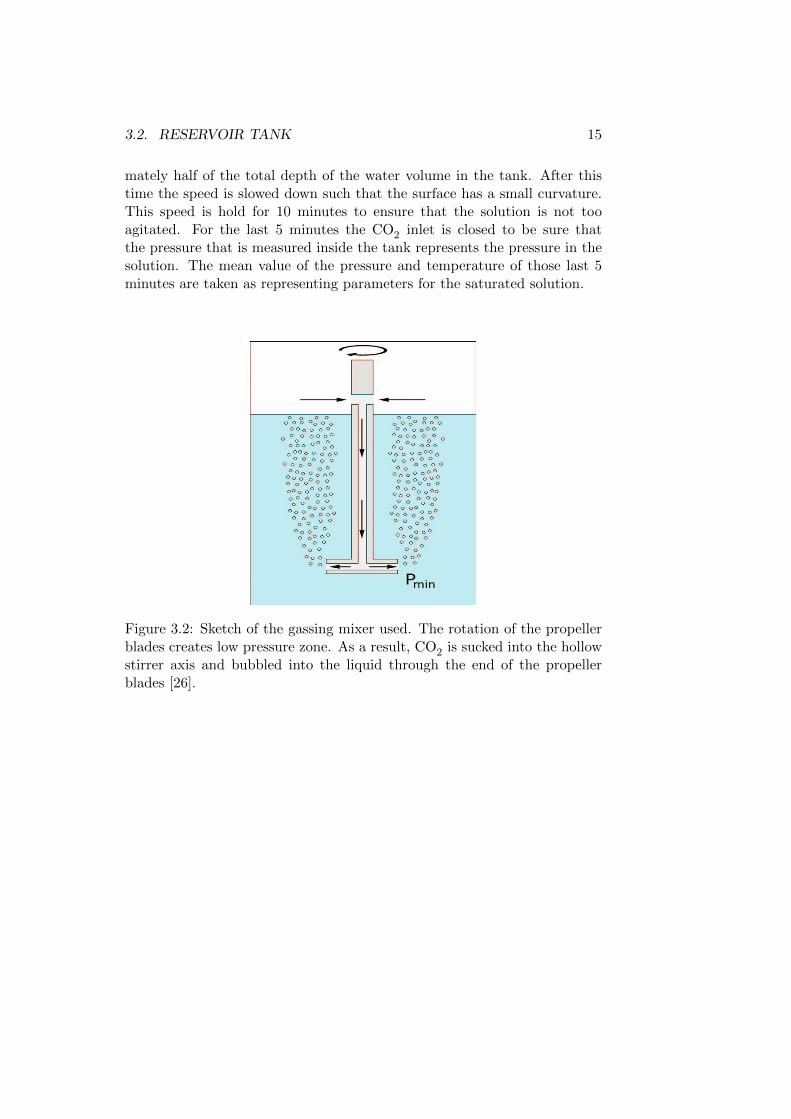
To prepare a solution of carbon dioxide and water the tank is first filledwith ultra pure water (MiliQ A10, Millipore) to a level such that there isenough space left for a gas layer on top. Then the liquid is exposed topressurized CO2 (provided by Linde Gas with 99.99% purity) of 0.65 MPa.The saturation process of the solution is accelerated by a stirrer attachedto a gassing propeller which is powered by a motor. Figure 3.2 shows howthe mixer acceleates the saturation process. The rotation of the propellerblades create a low pressure region around them. Due to this rotation gas issucked into the hollow stirrer axis and blown into the liquid through holesat the end of the propeller blades. With this mechanism it takes less than45 minutes to fully saturate the solution in this tank. The solution is leftovernight to allow the temperature to settle.

Before an experiment the solution is mixed for 35 minutes at a rate suchthat the depth of the vortex created by the stirring mechanism is approxi-

3.2. RESERVOIR TANK 15

mately half of the total depth of the water volume in the tank. After thistime the speed is slowed down such that the surface has a small curvature.This speed is hold for 10 minutes to ensure that the solution is not tooagitated. For the last 5 minutes the CO2 inlet is closed to be sure thatthe pressure that is measured inside the tank represents the pressure in thesolution. The mean value of the pressure and temperature of those last 5minutes are taken as representing parameters for the saturated solution.

Figure 3.2: Sketch of the gassing mixer used. The rotation of the propellerblades creates low pressure zone. As a result, CO2 is sucked into the hollowstirrer axis and bubbled into the liquid through the end of the propellerblades [26].


3.3 Observation tank

The observation tank is at the start of the procedure empty and at at-mospheric pressure. Before the tank is filled with solution, the chip withartificial nucleation site is blown dry with an air gun.

Then the tank is flushed with CO2 for 1 minute to expel atmosphericgasses. After this procedure the pressure is raised to the same value as inthe reservoir tank to avoid a sudden high pressure inflow of solution. Thevalves between the two tanks are then opened and water flows slowly intothe observation tank driven by the slightly higher position of the reservoirtank as shown in figure 3.3. A level switch ensures that the tank is alwaysfilled to the same level. After this procedure the solution is left to stabilizefor 3 minutes to ensure that the solution is quiescent.

camera

bubble

silicon chip withnucleation spot

pressureregulator 2

light

saturatedliquid

reservoir

pressureregulator 1

high pressureCO2

P2

pressureregulators

switch

valve

valve

P1

Figure 3.3: Sketch of the experimental set-up. With the pressure regulatorstwo different pressures can be provided: one to saturate the solution andanother to make the solution undersaturated. In the large thank the gasliquid solution is prepared and stored. Trough the system of steel pipesand pneumatic valves a portion of the solution can be transferred to theobservation tank. There the bubble can grow on a hydrophobic micro-pitetched on a silicon chip. The temperature in the system is kept stable bycirculating water from a refrigerated cooler through a hose wrapped aroundthe tank (see [26]). The process is visualised through a window in the tankusing a camera with a long-distance microscope objective with diffusive backlight at the opposite window.

3.4. EXPERIMENTAL SETTINGS 17

3.4 Experimental settings

The experiments are visualized by a camera with a long distance micro-scope objective. With custom made software, the images are acquired andprocessed. The images are saved at a frequency of 2 Hz and processed data(contour of the bubble) and the temperature and pressure of the observationtank are taken at a frequency of ∼ 5 Hz.

The bubbles are grown on a micro-sized pit with a radius of Rp = 50 µmand a depth of ∼ 30µm etched on a rectangular silicon chip (8 × 30 mm).A super-hydrophobic structure is present on the bottom of the pit in orderto ensure that gas will be entrapped inside the pit after being submerged inwater. This size of the pit is chosen in order to have a wide range of bubbleradii before the bubble detaches (maximal bubble radius before detachmentis Rdet ≈ 800 µm [20]).

To create an experiment that is reproducible the bubbles are grown toa predefined size. To define a size, the onset time where natural convectionplays a dominant role is taken into account because the growth rate will beenhanced due to natural convection [20]. For a bubble that grows after apressure drop of 0.10 MPa from the initial pressure of 0.65 MPa this onsettime is approximately 77 seconds [21, p. 49]. The sizes to which the bubblesgrew are chosen such that they are below, around and above this onset time.This correspond to bubbles with a radii of 90, 150 and 310 µm.

The bubble will grow in an oversaturated environment where the pres-sure is reduced 0.10 MPa form the initial pressure of 0.65 MPa. The finalsaturation states are chosen such that the bubble will dissolve due to surfacetension (PF = PI), dissolve due to undersaturated conditions (PF > PI) andto create a stable bubble (PF ≈ PI). All the experiments are done with atemperature of 20.2± 0.2 oC.

When the solution is stabilized in the observation tank the inflow ofCO2 is closed and the pressure switched to the other inlet if necessary. Therecording of the images and data points in the observation tank are startedat the same time in order to correlate the radius of the bubble with the rightpressure conditions. The pressure is lowered in a controlled way to createan oversaturated condition. After this pressure drop a bubble starts to growon the chip. When the bubble reached its defined size the CO2 inflow isopened again. The experiment is finished when the bubble fully dissolvedor the bubble started to grow after the second pressure change.


Experimental data of the pressure and radius are respectively shown infigure 3.4a and 3.4b for a final undersaturated solution.

The blue part represents the grow stage of the bubble (ζ ≈ 0.19), thegreen part dissolution mainly due to the pressure change and the red partdissolution mainly due to diffusion (ζ ≈ −0.18). In figure 3.5, 4 images ofthe lifetime of the bubble corresponding to those signals are shown.

P(M

Pa)

t (s)

0 50 100 150 200 250 3000.5

0.55

0.6

0.65

0.7

0.75

0.8

(a)

R(µm)

t (s)

0 50 100 150 200 250 30050

100

150

200

250

300

350

(b)

Figure 3.4: Experimental data for for the growth and dissolution of a CO2

bubble. a) Pressure as function of time, b) Radius as function of time.The solution is saturated at an initial pressure of PI = 0.639 MPa andtemperature TI = 20.2 oC. Three stages during the process are indicated:i) Growth during oversaturated conditions of ζ ≈ 0.19 (blue), ii) pressureincrease (green) and iii) dissolution during undersaturated conditions of ζ ≈−0.18 (red).

3.4. EXPERIMENTAL SETTINGS 19

R = 50 mμ t = 24 s R = 314 mμ t = 176 s

R = 225 mμ t = 190 s R = 140 mμ t = 246 s

Figure 3.5: Pictures of the different stages during bubble growth and disso-lution corresponding to the data in figure 3.4. Top left picture is the momentwhen the bubble is a hemisphere (corresponding to the first point in figure3.4b). The top right picture is the moment where the predefined radius isreached. Bottom left picture is the first moment that the pressure reachedits final value. Bottom right picture is 56 seconds after the pressure hasreached its final value.

Chapter 4

Theoretical aspects

In this chapter the theoretical relation for the evolution of the radius of agas bubble on a substrate in a gas-liquid solution with different saturationconditions will be derived. To do so, first the ideal situation as formulatedby Epstein and Plesset will be explained. Then a factor will be given todetermine the effective area for mass transfer. Finally we derive a “historyterm” to account for the effects of the concentration profile in the dissolutionof the bubble. After the derivation an explanation will be given about how itis implemented in a numerical model.

4.1 Idealized situation

Epstein and Plesset define an idealized problem where a bubble grows or dis-solves due to diffusion in an unbounded and isothermal respectively, over-or undersaturated gas-liquid solution. The initial equilibrium concentrationof the solution is given by CI = kHPI at a temperature TI (Henry’s law).When the pressure is changed this leads to an out of equilibrium state thatcan be over- or undersaturated. At t = 0 a spherical bubble with an initialradius R0 will be placed in this gas-liquid solution. The concentration onthe boundary of the bubble can be given by CS = kHPS (at the same tem-perature TI). The center of the bubble remains at the origin of a sphericalcoordinate system.

21

22 CHAPTER 4. THEORETICAL ASPECTS

4.2 Pressure changes

The experimental situation differs in the fact that the pressure is not con-stant but changes during the experiment. To analyse only the change inradius due to diffusion the experimental data is multiplied by a factor thatcompensates for the pressurese changes. This factor is deduced from theideal gas law which states: PV = constant. The initial pressure PI is takenas ambient pressure in the gas-liquid solution because the liquid is saturatedas this pressure. So the compensated radius will be given by;

R∗(t) = R(t) 3

√P (t)

PI, (4.1)

were R(t) is the measured radius, P (t) the pressure at the same time andPI the initial pressure of the bulk of the solution.

4.3 Influence of the chip

In the ideal case the bubble grows or dissolves in an infinite medium but inthe experimental case the bubble grows on a substrate. Therefore the masstransfer is reduced in the experimental case. This is caused by two effects:1) The bubble can not be treated as spherical because it does not grow muchlarger than the pit radius, and 2) The chip acts like a barrier which hindersmass transfer into or out of the bubble. Those effects can qualitativelybe estimated by removing the mass diffusing across the dashed area of thebubble surface shown in figure 4.1, where the larger sphere represents theedge of the boundary layer of thickness δ =

√πDt. With a simple geometric

calculation the “effective” area can be determined that remains for masstransfer. This area is given by:

Aeff = 4πR2

1

2+

1

2

√1−

(Rp

R

)2

1 + δR

= 4πR2fA(t) (4.2)

When the mass transfer at the boundary of the bubble is determined theeffective area Aeff has to be used instead of the full bubble surface. This isthe same as multiplying the equation for mass transfer by factor fA.

4.4. FORMULATION OF THE DIFFUSIVE PROBLEM 23

R

bubble

boundary layer

silicon chip

Rp

CS

δ

CI

Figure 4.1: Sketch to illustrate the interaction of the boundary layer withthe silicon chip and the fact that the bubble can not be treated as a sphere.The excluded bubble area (dashed line) is estimated using the cone formedby the center of the bubble and intersection of the boundary layer (shownby the bigger sphere) with the silicon chip.

4.4 Formulation of the diffusive problem

We start with the ideal situation as described by Epstein and Plesset. Thegas concentration C, obeys the convection-diffusion equation,

∂tC + R(t)R(t)2

r2∂rC = D

1

r2∂r(r

2∂rC) (4.3)

with the boundary conditions:

r = R(t) : C(R(t), t) = CS(t) + kH2σ

R= kH

(P (t) +

2σ

R

)(4.4)

R→∞ : C(∞, t)→ CI (4.5)

and the initial condition: C(r, 0) = CI . Henry’s law is applied on the pres-sure that is present on the boundary of the bubble. This pressure consists ofthe gas pressure P (t) and the Laplace pressure 2σ/R, where σ = 0.069 N/mis the surface tension of the gas-liquid interface. The diffusion constant isD = 1.97× 10−9 m/s2

By using the arguments of Epstein and Plesset [22] the convective termwill be neglected. This condition is well justified when Peclet number issmall Pe = RR/D � 1. So with this assumption equation 4.3 transformsinto:

∂tC = D1

r2∂r(r

2∂rC) (4.6)


The problem will made dimensionless using the following rescaled

radial coordinate ξ =r

R(t)(4.7a)

time change dτ = dtD

R(t)2(4.7b)

concentration c(τ) =C(t)

CI− 1 (4.7c)

radius a(τ) =R(t)

RI(4.7d)

Where R0 is the radius at t = 0 this radius is not defined in the experimentsso another length scale have to be defined.

When those dimensionless parameters are used to make equation 4.6dimensionless and neglecting therms of order O(Pe) (see appendix A), theproblem could be written as:

∂τ c =1

ξ2∂ξ(ξ

2∂ξc) (4.8)

with the boundary conditions:

ξ = 1 : c(1, τ) = cS(τ) =CS + kH

2σR

CI− 1

=cS(τ) +kHCI

2σ

a(τ)R0

=cS(τ) +η

a(τ)R0(4.9)

ξ →∞ : c(∞, t)→ 0 (4.10)

and the initial condition c(ξ, 0) = 0. For brevity in the above and furtherexpressions we use cS = CS/CI − 1 and η = 2σkH/CI .

The solution will be sought in the form c(ξ, τ) = f(ξ, τ)/ξ. From equa-tion 4.8 this function, f , satisfies:

∂τf = ∂ξξf (4.11)

With this equation we want to obtain an expression for the mass flowacross the bubble surface (ζ = 1). To do so the Laplace transform of equa-tion 4.11 is taken. Taking into account the initial condition f(ξ, 0) = 0 givesthe differential equation:

sf =d2f

dξ2(4.12)

This equation can be solved in combination with boundary conditions 4.9and 4.10, which gives the following solution:

f(ξ, s) = ˆcSe−√s(ξ−1) (4.13)

4.5. EPSTEIN-PLESSET EQUATION WITH HISTORY TERM 25

To compute the mass flux across the bubble surface (ξ = 1), it sufficesto evaluate:

∂ξ c|ξ=1 = f ′(1, s)− f(1, s) = −√sˆcS − ˆcS (4.14)

This expression can be transformed back to the time domain using the con-volution theorem:

∂ξc|ξ=1 = −L−1

[1√ssˆcS

]− cS = −

∫ τ

0

1√π(τ − τ ′)

dcSdτ ′

dτ ′ + cS (4.15)

The part within the integral describes the influence of the concentrationin the boundary layer on the flux across the bubble surface and is thereforecalled the history term. The other term is the flux induced by the relativedifference in concentration between the concentration on the bubble surfaceand the concentration of the bulk solution. In the history term is used cSis used instead of cS = cS + η

aR0. This replacement can be done because

dcS/dτ ≈ dcS/dτ for bubbles of micrometer scale.

4.5 Epstein-Plesset equation with history term

A similar expression to the Epstein-Plesset equation will be derived for thereal situation (including the influence of the chip) from the equation formass conservation. Laplace pressure is taken into account in this derivationand the gas inside the bubble is treated as ideal,

dm

dt=

d

dt

(4

3πR(t)3ρ(t)

)= 4πR2DfA(t)∂rC|r=R (4.16)

where ρ(R(t)) is the gas density inside the bubble. This density will bededuced from the ideal gas law and in combination with the assumptionthat the process is isothermal the relation becomes:

M

kHBT

(R

3CS + CSR+

4

3σkH

R

R

)= DfA(t)∂rC|r=R, (4.17)

where M is the molar mass of CO2 and B the ideal gas constant. The di-mensionless parameters as defined in 4.7 are used to make the above equationdimensionless. An equivalent to the Epstein-Plesset equation in dimension-less form is then given by:

da

dτ= − a

(cS + 1) + 23

ηaR0

{ΛfA(τ)

[∫ τ

0

1√π(τ − τ ′)

dcSdτ ′

dτ ′ + cS

]+

1

3

dcSdτ

}(4.18)


where Λ = kHBT/M and the area correction factor for the effective area isgiven by:

fA(τ) =1

2+

1

2

√1−

(Rp

a(τ)R0

)2

1 +√πτ

, (4.19)

with Rp the radius of the pit.The da/dτ of equation 4.18 is given by 3 components:

history effects − a

(cS + 1) + 23

ηaR0

ΛfA(τ)

∫ τ

0

1√π(τ − τ ′)

dcSdτ ′

(4.20a)

concentration − a

(cS + 1) + 23

ηaR0

ΛfAcS (4.20b)

concentration difference − a

(cS + 1) + 23

ηaR0

1

3

dcSdτ

(4.20c)

Equation 4.20a is called the history term because the influence of theconcentration profile in the boundary layer is taken into account. The secondcomponent (equation 4.20b) describes the contribution due to the relativedifference in concentration at the surface of the bubble and in the bulk ofthe solution. The third component describes the contribution of the relativechange of the concentration in time at the bubble surface.

4.6 Numerical simulations

The integral equation derived in the previous subsection (equation 4.18),will be used in an algorithm with the appropriate boundary conditions tosimulate the theory. The integral will be evaluated using the algorithmsuggested by Elghobashi et al. [27] for the Basset force in the motion ofsolid particles through a liquid. The solution of those simulations will becompared with the experimental results.

The experiments are comparable from the moment that the size of thebubble is such that it is equal to a hemisphere with radius R∗ = 50 µm.Therefore the scaling radius is chosen to be R0 = 50 µm.

As can be seen figure 3.4 the bubble reades a radius of 50 µm after thepressure is dropped to its lowest value. However the simulation needs a dou-ble pressure drop to represent the theory. Therefore a pressure drop of 0.10MPa is used that has approximately the same dimensions as in the exper-iments as shown in figure 4.2a. The experimental pressure P (t) is used tocompute a representative pressure profile p(τ) for the simulations from themoment the pressure starts to rise. The experimental radius R∗(t) had tobe used to obtain the right conversion from t→ τ because the dimensionlesstime increase is given by 4.7b. In figure 4.2b is shown the comparison of the

4.6. NUMERICAL SIMULATIONS 27

experimental and numerical data for the pressure increase where the latterhas been converted back from τ to t. A small difference can be observed be-tween the two graphs, which is likely to be caused by the conversion t↔ τ .The dimensionless radius a(τ) is multiplied by R0p(τ)/p(0) to compensatefor the pressure changes and the signal is then transformed back to the timedomain such that it can be compared with the experimental radius. Thetime between the two pressure changes (in the numerics) is adjusted suchthat the maximal radii of the experiments and numerical solution happen atthe same point in the t-domain. The maximal radius has been chosen as thestarting point for the comparison between the simulations and the experi-ments because the initial radius and the exact time when the bubble startsgrowing in experiments cannot be precisely determined due to the fact thatthe bubble initially grows inside the pit. This will lead to a mismatch in theboundary layer size of around 20% (for the case shown in figure 4.2) whichmight be one of the reasons behind the differences between experimentaland numerical results.

The radius as function of time is shown in figure 4.3a for the experimen-tal and numerical data . From this figure is clear that the growth in thenumerical case takes a bit longer than in the experimental case (from themoment R∗ = 50 µm) but is of the same order. The differences may becaused by the initial conditions that are chosen. In this research the focuswas on the dissolution process after the bubble has grown in an oversatu-rated solution. Therefore graphs are shifted such that t = 0 represents themoment that the pressure starts to increase because that is the moment thatthe radius has reached its maximum value. An illustration of this is givenin figure 4.3b.


numerical

experiment

P(M

Pa)

t (s)

0 10 20 30 40 50 60 70 800.5

0.55

0.6

0.65

0.7

0.75

0.8

(a)

numerical

experiment

P(M

Pa)

t (s)

0 10 20 30 40 50 60 70 800.5

0.55

0.6

0.65

0.7

0.75

0.8

(b)

Figure 4.2: Experimental and numerical data for the pressure as functionof time. a) t = 0 is equal to the moment that the experimental pressuredecreases. The numerical pressure is adjusted such that the time to decreasesis approximately the same. b) t = 0 is equal to the moment where R∗ =50 µm. The numerical and experimental profiles are placed on top of eachother to show that the pressure increase is approximately the same.

4.6. NUMERICAL SIMULATIONS 29

numerical

experimental

R∗ (µm)

t (s)

0 10 20 30 40 50 60 70 80

60

80

100

120

140

160

(a)

numerical

experimental

R∗ (µm)

t (s)

0 5 10 15 20 25 30 35

60

80

100

120

140

160

(b)

Figure 4.3: Experimental and numerical data for the radius as functionof time. a) t = 0 correspond to the moment where R∗ = 50 µm. Thepressure profile is adjusted such that the maximal radii are approximatelythe same. b) t = 0 correspond to the moment where R∗ is maximal. Thisrepresentation provides the best insight in the dissolution process.

Chapter 5

Results

In this chapter the results of the experiments are discussed and comparedto the corresponding numerical simulations. In the first section dissolutionunder final undersaturated conditions will be treated. Here, the influenceof convection on the dissolution process becomes visible. It is followed by asection where the final conditions are saturated. In the final section it willbe addressed how a stable bubble can be produced.

5.1 Bubble behaviour in anundersaturated solution

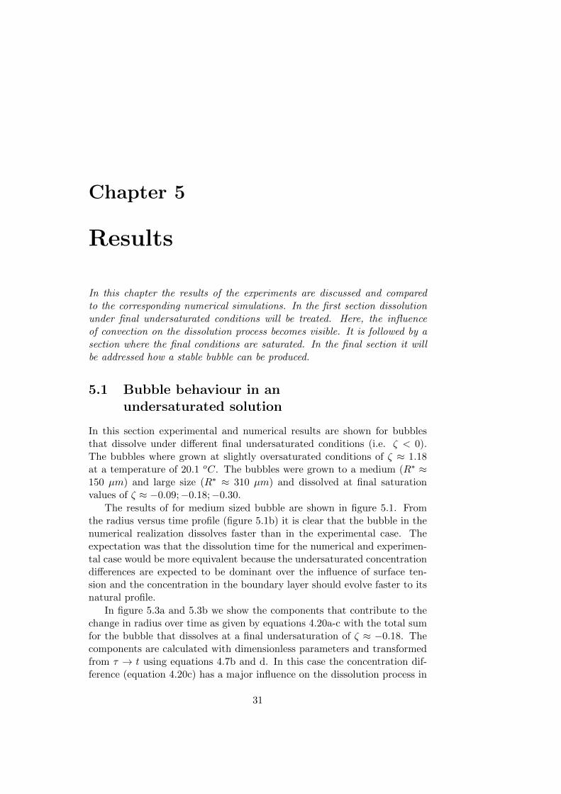
In this section experimental and numerical results are shown for bubblesthat dissolve under different final undersaturated conditions (i.e. ζ < 0).The bubbles where grown at slightly oversaturated conditions of ζ ≈ 1.18at a temperature of 20.1 oC. The bubbles were grown to a medium (R∗ ≈150 µm) and large size (R∗ ≈ 310 µm) and dissolved at final saturationvalues of ζ ≈ −0.09;−0.18;−0.30.

The results of for medium sized bubble are shown in figure 5.1. Fromthe radius versus time profile (figure 5.1b) it is clear that the bubble in thenumerical realization dissolves faster than in the experimental case. Theexpectation was that the dissolution time for the numerical and experimen-tal case would be more equivalent because the undersaturated concentrationdifferences are expected to be dominant over the influence of surface ten-sion and the concentration in the boundary layer should evolve faster to itsnatural profile.

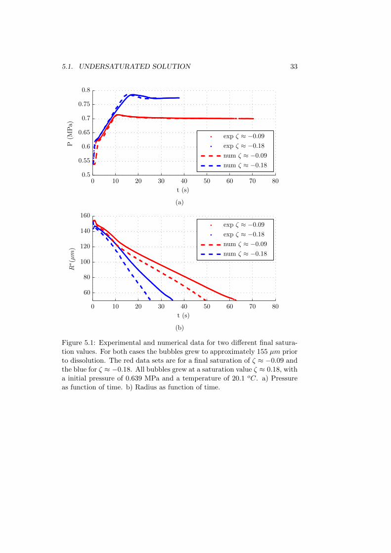
In figure 5.3a and 5.3b we show the components that contribute to thechange in radius over time as given by equations 4.20a-c with the total sumfor the bubble that dissolves at a final undersaturation of ζ ≈ −0.18. Thecomponents are calculated with dimensionless parameters and transformedfrom τ → t using equations 4.7b and d. In this case the concentration dif-ference (equation 4.20c) has a major influence on the dissolution process in

31

32 CHAPTER 5. RESULTS

the time frame when the pressure raise (t ≈ 0−30 seconds). The concentra-tion change over time also has influence on the history term (equation 4.20a)due to the integration over this derivative of the concentration over the totalelapsed time. The contributions of the concentration differences (equation4.20b) and the history term are in the same order during t ≈ 12−22. There-after the change in radius is dominated by the concentration differences, asexpected. From the same figures it becomes clear that the experimental re-sults are between the contribution of the history effects and the total sum ofthe components. This could be caused by the fact that in the experimentalcase the boundary layer is larger and therefore the influence of the historyeffects is smaller.The large bubble has a growth time that sure passes the time where naturalconvection becomes dominant (tgrow > 77 seconds). Therefore the mass flowis larger during the growth stage than without this dominant term. Natu-ral convection is not included in the simulations and therefore the growthtime in the simulations has to be extended more than in the other cases.In figure 5.2 the pressure and radius data are given for the three differentfinal saturation conditions. The differences in the numerical and experi-mental dissolution times are relatively larger compared to the results of themedium bubble. This larger difference can be explained with the parts thatcontribute to the radial change in time that is shown in figure 5.3b and thedescription of the concentration profile in the boundary layer given in thesecond chapter. When the process is dominated by diffusion the concen-tration profile in the boundary can be represented in a simplified mannerby the profile shown in figure 2.3b. In this case the bubble feels a locallyundersaturated condition that is larger than the final new equilibrium un-dersaturation. The net mass flow from the bubble to the surroundings willtherefore be larger until an natural profile has established. This concentra-tion profile is disturbed when convection becomes dominant and thereforethe effect of the locally undersaturation within the boundary layer will bediminished. This means that the mass flow from the bubble to the sur-roundings will be smaller. This effect is visible in the results because in thenumerical simulations the concentration profile is intact (no convection in-cluded) and this bubble dissolves faster than the experiments. In figure 5.3bis also visible that the contribution of the history term has influence over along time frame (∼ 50 seconds) before the concentration difference (cS) isdominant in the radial change. This would not be the case if the boundarylayer was mixed due to convection and the radial change over time wouldbe smaller.

5.1. UNDERSATURATED SOLUTION 33

num ζ ≈ −0.18

num ζ ≈ −0.09

exp ζ ≈ −0.18

exp ζ ≈ −0.09

P(M

Pa)

t (s)

0 10 20 30 40 50 60 70 800.5

0.55

0.6

0.65

0.7

0.75

0.8

(a)

num ζ ≈ −0.18

num ζ ≈ −0.09

exp ζ ≈ −0.18

exp ζ ≈ −0.09

R∗ (µm)

t (s)

0 10 20 30 40 50 60 70 80

60

80

100

120

140

160

(b)

Figure 5.1: Experimental and numerical data for two different final satura-tion values. For both cases the bubbles grew to approximately 155 µm priorto dissolution. The red data sets are for a final saturation of ζ ≈ −0.09 andthe blue for ζ ≈ −0.18. All bubbles grew at a saturation value ζ ≈ 0.18, witha initial pressure of 0.639 MPa and a temperature of 20.1 oC. a) Pressureas function of time. b) Radius as function of time.


num ζ ≈ −0.30

num ζ ≈ −0.18

num ζ ≈ −0.09

exp ζ ≈ −0.30

exp ζ ≈ −0.18

exp ζ ≈ −0.09P

(MPa)

t (s)

0 50 100 150 200 2500.5

0.6

0.7

0.8

0.9

(a)

exp ζ ≈ −0.30

exp ζ ≈ −0.18

exp ζ ≈ −0.09

R∗ (µm)

t (s)

0 50 100 150 200 25050

100

150

200

250

300

(b)

Figure 5.2: Experimental and numerical data for two different final satura-tion values. For both cases the bubbles grew to approximately 300 µm priorto dissolution. The red data sets are for a final saturation of ζ ≈ −0.09,the blue for ζ ≈ −0.18 and the green for ζ ≈ −0.30. All bubbles grew at asaturation value ζ ≈ 0.18, with a initial pressure of 0.639 MPa and a tem-perature of 20.1 oC. a) Pressure as function of time. b) Radius as functionof time.

5.1. UNDERSATURATED SOLUTION 35

exp total

dcS/dt-part

cS

history

num total

dR

∗

dt

(µm s)

t (s)

0 10 20 30 40 50−12

−10

−8

−6

−4

−2

0

2

(a)

exp total

dcS/dt-part

cS

history

num total

dR

∗

dt

(µm s)

t (s)

0 10 20 30 40 50 60 70 80 90−12

−10

−8

−6

−4

−2

0

2

(b)

Figure 5.3: Components of the derivative (given by equation 4.20) of theradius as function of time from the numerical simulation combined withexperimental results for a bubble that grow at ζ ≈ 0.18 and dissolved ata final ζ ≈ −0.18. a) Results for bubble with a medium size and b) largesize. The first negative peak in both graphs is caused by the inital pressurejump from the lowest pressure to approximately the initial pressure. Thedecreasing ratio after this peak is caused by the overshoot of the pressureregulator.


5.2 Bubble behaviour in asaturated solution

In this section experimental and numerical results are shown for bubbles thatdissolves under conditions that are close to complete saturation (ζ ≈ 0.005).The bubbles where initially grown at oversaturated conditions of ζ ≈ 0.18at a temperature of 20.2 oC to radii R∗ ≈ 100 µm and R∗ ≈ 160 µm whichare respectively called a small and a medium sized bubble. The marginallyoversaturated conditions of the experiments (ζ ≈ 0.005) could not be usedin the numerical simulation because the bubble would eventually start togrow. Therefore the initial (saturation) pressure in the numerical case ischosen such that the solution becomes completely saturated (i.e. ζ = 0) ata constant temperature of 20.2 oC.

The radius as function of time for both sizes are shown in figure 5.4b. Inthis figure can be seen that the numerical solution needs longer to dissolvethan in the experiments. In the same figure it is also visible that the bubblesstill grow when the pressure is raised what was not observed during theexperiments discussed in the previous section.

The growth of the bubble after the pressure starts to increase is caused bythe long duration of this increase, as can be seen in figure 5.4a. In figure 5.5all the components that contribute to dR∗/dt are shown. The concentrationcomponent (equation 4.20b) is positive during the pressure increase becausethe solution is still oversaturated (−0.18 < ζ < 0). The concentration profilein the boundary layer also changes slowly and at a certain moment the massflux caused by this profile changes form into to out of the bubble as can beseen by the history term (equation 4.20a). The sum of all three componentscauses that the bubble start to dissolve approximately 30 seconds after thepressure started to increase. This behaviour is visible in the experimentaland numerical data of radius versus time as shown in figure 5.6 where thedifferent pressure regions are indicated.

The numerical radius has a size of 154 µm when the pressure reached itsstable value. The dissolution of a bubble of this size in the ideal case as Ep-stein and Plesset described it is approximately 3000 seconds. The substratehas a large influence slowing down the mass transfer. When correcting thisdissolution time with a maximal area factor of 0.686 [28], the dissolutiontime becomes approximately 4400 seconds. This time is in good agreementwith the numerical dissolution time.

The main difference between dissolution of the ideal case and this caseis that there is a pre-existing concentration profile present at the momentthe bubble starts to dissolve. The components of dR∗/dt after the pressurereached its stable value are shown in figure 5.5b. In this figure is visible thatthe history term (equation 4.20a) has a large influence on the total changein radius from 100 till 200 seconds. The concentration component (equation

5.2. SATURATED SOLUTION 37

4.20b) is dominant after 500 seconds. This is caused by the fact that thebulk concentration with respect to the bubble surface concentration due tothe gas pressure inside the bubble is zero (i.e. cS = 0 and dcS/dt = 0). Thismeans that a equilibrium concentration profile will establish in the bound-ary layer (i.e. history term → 0) and the concentration difference is givenby surface tension (i.e. cS = η/(aR0)).The history term plays a role in the dissolution process but it does notexplain the large differences. The numerical model is very sensitive for con-centration changes (i.e. pressure and temperature changes) so for a bettercomparison those changes have to be taken into account during the wholesimulation.


numerical

experiment

P(M

Pa)

t (s)

0 100 200 300 400 500 600 700 8000.54

0.56

0.58

0.6

0.62

0.64

0.66

(a)

numerical

experiment

numerical

experiment

R∗(µm)

t (s)

0 1000 2000 3000 4000

60

80

100

120

140

160

(b)

Figure 5.4: a) pressure as function of time for experimental and numericalcase. b) radius as function of time for two experiments where the bub-ble grew to approximately R∗ ≈ 160 µm (red) and R∗ ≈ 100 µm (blue).The final saturation value in the experimental cases was ζ = 0.005. Theexperiments are compared with numerical simulation where the final satu-ration was ζ = 0.000 . The bubbles grew at oversaturated conditions withζ ≈ 0.180 with a temperature of T = 20.2 oC

5.2. SATURATED SOLUTION 39

dcS/dt-part

cS

history

num total

dR

∗

dt

(µm s)

t (s)

0 20 40 60 80 100−0.5

0

0.5

1

1.5

2

(a)

dcS/dt-part

cS

history

num total

dR

∗

dt

(µm s)

t (s)

100 200 300 400 500 600 700 800−0.08

−0.06

−0.04

−0.02

0

0.02

(b)

Figure 5.5: The different contributions to the derivative of the radius in timefor the medium bubble under saturated final conditions. The componentscorrespond with equations 4.20a-c). a) for the first 100 seconds. b) from 100till 800 seconds. During pressure raise all components give a contribution.The first 100 seconds when the pressure is stable the history term is dom-inant. After a wile the history term tend to zero and cS (which representsthe surface tension in this case) becomes dominant. The peaks around 2 iscaused by the fact that the numerical and experimental pressure profile arecombined when the pressure starts to rise and the peak around 230 is causedby a small compensation due to the pressure regulator in the system.


num PF

num PR

exp PF

exp PR

R∗(µm)

t (s)

0 50 100 150 200 250 300 350 400120

130

140

150

160

Figure 5.6: Experimental and numerical data for a medium sized bubbleR ≈ 160 µm for radius versus time. Two regions are indicated: green)pressure increase red) stable final pressure (where ζ = 0.005 in for theexperiments and ζ = 0.000 for the numerical calculations )

5.2. MARGINALLY OVERSATURATED SOLUTION 41

5.3 Bubble behaviour in amarginally oversaturated solution

The most challenging task is to try to stabilize a bubble. In the ideal case thesaturation has to be such that it compensates the Laplace pressure presentdue to the surface tension between the gas air interface. This pressure is fora bubble of 90 µm only 1.52 kPa which is below the precision of the pressureregulators of the experimental set-up.

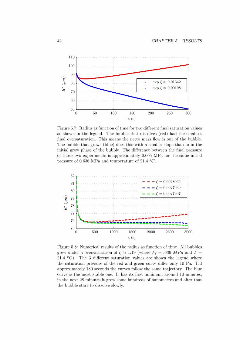
From the experiments described in the previous sections it could beconcluded that the applied conditions also have to compensate for the historyterm in the boundary layer. Therefore experiments were done where the finaland initial pressure differ only 10 kPa or less. The pressure raise was madefaster (about 3 seconds) to ensure that the bubble dissolve a bit duringthe pressure raise. The experimental results are shown in figure 5.7 forthe dissolution of a small bubble that grew under oversaturated conditionsof ζ ≈ 0.19 with a initial pressure of 0.636 MPa and a temperature of21.4 oC. The final saturation values of those experiments are marginallyoversaturated ζ = 0.01342 and ζ = 0.00198. The differences between thefinal pressure of those two experiments is only 5 kPa and it gave a totallydifferent result.

Numerical calculations are made with the same initial and growth con-ditions as in the experiments. The final pressure is adjusted such that astable bubble is created as can be seen in figure 5.8. The fast pressure raiseinduce a large change in the concentration profile of the boundary layer.Therefore the history term (equation 4.20a that describe the effects due tothose changes) is dominant for the bubble behaviour for the first 3 to 10minutes. After that moment there is still a sensitive balance between thehistory term and the concentration component (equation 4.20b). The nu-merical calculation made with saturation value of ζ = 0.0027939 has themost stable results. The difference between the initial and final pressure isin this case 1.77 kPa. This is close to the Laplace pressure of a bubble witha radius of 76 µm which is 1.80 kPa, which illustrates the marginally smallpressure differences that have to be compensated. The experimental equip-ment would have to be more sensitive and the pressure would have to beadjustable during the stabilization process to compensate for those historyeffects.


exp ζ ≈ 0.00198

exp ζ ≈ 0.01342

R∗(µm)

t (s)

0 50 100 150 200 250 30050

60

70

80

90

100

110

Figure 5.7: Radius as function of time for two different final saturation valuesas shown in the legend. The bubble that dissolves (red) had the smallestfinal oversaturation. This means the netto mass flow is out of the bubble.The bubble that grows (blue) does this with a smaller slope than in in theinitial grow phase of the bubble. The difference between the final pressureof those two experiments is approximately 0.005 MPa for the same initialpressure of 0.636 MPa and temperature of 21.4 oC.

ζ = 0.0027907

ζ = 0.0027939

ζ = 0.0028066

R∗(µm)

t (s)

0 500 1000 1500 2000 2500 300075

76

77

78

79

80

81

82

Figure 5.8: Numerical results of the radius as function of time. All bubblesgrew under a oversaturation of ζ ≈ 1.19 (where PI = .636 MPa and T =21.4 oC). The 3 different saturation values are shown the legend wherethe saturation pressure of the red and green curve differ only 10 Pa. Tillapproximately 180 seconds the curves follow the same trajectory. The bluecurve is the most stable one. It has its first minimum around 10 minutes,in the next 28 minutes it grow some hundreds of nanometres and after thatthe bubble start to dissolve slowly.

Chapter 6

Discussion and Conclusion

The goal of this research was to investigate the dissolution process of a CO2

bubble that dissolved conditions of saturation after it first was grown in aslightly oversaturated environment.

This process was only described by Epstein and Plesset for an idealsituation where a pre-existing gas bubble dissolved in an infinite gas-liquidsolution with a certain constant saturation value. A new relation, thatis comparable with the combination of Epstein and Plesset equations forgrowth and dissolution, was derived that could describe the process withthe conditions used during the experiments.

First, experiments where carried out with under saturated condition.The numerical simulation predicted that the bubble should now dissolvemainly due to surface tension. In the experiment the bubble dissolved fasterthan the theory and in addition we found that the reproducibility of theexperiments was quite bad.

The second series of experiments that where carried out with various un-dersaturated conditions were reproducible. The numerical dissolution timewas in the same order but slightly faster than the experimental results. Theratio of the experimental and numerical dissolution time became higher fora bubble that grew partly dominated by natural convection compared toa bubble that grew mainly due to diffusion. This indicates that for bothsituations convection may play a role in the dissolution process.

Finally, experiments with a final marginally oversaturation were carriedout to investigate if it was possible to create a stable bubble. From theexperimental results and numerical simulation it became clear that the finalpressure should be varied in a sensitive way to compensate for the Laplacepressure and history effects.

For the numerical simulation of the theory several parameters had to bechosen or estimated (scaling radius, surface tension, initial pressure drop).The simulations where done under such conditions that mimic the realitythe best. Especially for bubble behaviour under saturated conditions we

43

44 CHAPTER 6. DISCUSSION AND CONCLUSION

saw that it was sensitive to small concentration differences. More researchhave to be done to know if the assumption of a constant temperature canbe justified.

In further research convection should be included in the derivation ofthe theoretical equation and there have to be checked if the assumption ofa constant temperature can be justified (even tough the changes are small).The experiments could be carried out at a smaller scale to have a largerinfluence of surface tension and the experimental set-up can be improvedwith a device to regulate the pressure during the experiment.

Appendix A

Full dimensionlessconvection-diffusion equation

In this appendix the full dimensionless equation will be derived for therescaled gas concentration, c(ζ, τ) without the assuming Pe� 1. The termsof equation 4.3 becomes are stated below when the dimensionless parametersfrom equation 4.7.

∂tc = ∂tτ∂τ c =D

R20

1

a2

(∂rc−

a′

aξ∂ξc

)(A.1)

RR2

r2∂rc =

D

R20

1

a2

a′

a

∂ξc

ξ2(A.2)

D

r2∂r(r2∂rc

)=

D

ξ2a2R20

∂rξ∂ξ(ξ2a2R2

0∂rξ∂ξc)

=D

R20

1

a2

1

ξ2∂ξ(ξ

2∂ξc) (A.3)

Combining those expression give,

∂τ c+a′

a

(1

ξ2− ξ)∂xic =

1

ξ2∂xi(ξ

2∂ξc) (A.4)

Where a = da/dt, this therm is proportional to the Peclet number a′ =RRR0D

∼ Pe� 1and therefore the terms with a′ can be neglected.

45

46APPENDIX A. FULL DIMENSIONLESS CONVECTION-DIFFUSION EQUATION

Bibliography

[1] M. Amon and C. D. Denson. A study of the dynamics of foam growth:Analysis of the growth of closely spaced spherical bubbles. PolymerEngineering and Science, 24(13):1026–1034, 1984.

[2] C. B. Park and L. K. Cheung. A study of cell nucleation in the extrusionof polypropylene foams. Polymer Engineering & Science, 37(1):1–10,1997.

[3] S. A. Thorpe. On the clouds of bubbles formed by breaking wind-wavesin deep water, and their role in air-sea gas transfer. The Royal Society,304, 1982.

[4] J.W. Westwater J.P. Glas. Measurements of the growth of electrolyticbubbles. International Journal of Heat and Mass Transfer, 7(12):1427–1430, 1964.

[5] T. van Terwisga B. Wieneke E. J. Foeth, C. W. H. van Doorne. Timeresolved piv and flow visualization of 3d sheet cavitation. Experimentsin Fluids, 40(4):503–513, 2006.

[6] S. Fang Z. Zhua. Numerical investigation of cavitation performance ofship propellers. Journal of Hydrodynamics, Series B, 24(3):347–353,2012.

[7] W. L. Korff S. N. Patek and R. L. Caldwell. Biomechanics: Deadlystrike mechanism of a mantis shrimp. Nature, 428:819–820, 2004.

[8] D. E. Yount and R. H. Strauss. Bubble formation in gelatin: A modelfor decompression sickness. Journal of Applied Physics, 47:5081–5089,1976.

[9] C. Balestrad T.D. Karapantsiosc V. Papadopouloua, R.J. Eckersleyband M-X Tanga. A critical review of physiological bubble formation inhyperbaric decompression. Advances in Colloid and Interface Science,191:22–30, 2013.

[10] W. Yang. Dynamics of gas bubbles in whole blood and plasma. Journalof Biomechanical Engineering, 4:119–125, 1971.

47

48 BIBLIOGRAPHY

[11] H. D. Van Liew and S. Raychaudhuri. Stabilized bubbles in the body:pressure-radius relationships and the limits to stabilization. Journal ofApplied Physiology, 82:2045–2053, 1997.

[12] E.L. Jack A. Lachmann and D.H. Volman. Isothermal and isobaricdegassing of ice cream. Industrial & Engineering Chemistry, 42(2),1950.

[13] G.M. Evans S.F. Jones and K.P. Galvin. Bubble nucleation from gascavities a review. Advances in Colloid and Interface Science, 80:27–50,1999.

[14] J. S. McKechnie W. T. Lee and M. G. Devereux. Bubble nucleation instout beers. Physical Review E: Statistical, Nonlinear, and Soft MatterPhysics, 83:051609, 2011.

[15] A. N. Gent and D. A. Tompkins. Surface energy effects for small holesor particles in elastomers. Journal of Polymer Science, Part B: PolymerPhysics, 7(9):1483–1487, 1969.

[16] D. Wang X. Zhang, D.Y. C. Chan and N. Maeda. Stability of interfacialnanobubbles. Langmuir, 13:1017–1023, 2013.

[17] J. H. Weijs and D. Lohse. Why surface nanobubbles life for hours.Physical Review Letters, 110, 2013.

[18] D. Lohse and X. Zhang. Pinning and gas oversaturation imply stablesingle surface nanobubbles. Physical Review Letters, 91, 2015.

[19] C. Voisin G. Liger-Belair and P. Jeandet. Modeling nonclassical het-erogeneous bubble nucleation from cellulose fibers; application to bub-bling in carbonated beverages. Journal of Physical Chemistry B,109:1457314580, 2005.

[20] D. Lhse A. Prosperetti O.R. Enrıquez, C. Sun and D. van der Meer.The quasistatic growth of CO2 bubbles. Journal of Fluid Mechanics,741, 2014.

[21] O.R. Enrıquez. Growing bubbles and freezing drops: depletion effectsand tip singularities. PhD thesis, Universiteit Twente, Enschede, 2015.

[22] P.S. Epstein an d M.S. Plesset. On the stability of gas bubbles inliquid-gas solutions. Journal of Chemical Physics, 18, 1950.

[23] M. Cable. The dissolving of stationay gas bubbles in a liquid. ChemicalEngineering Science, 22:1393–1398, 1967.

BIBLIOGRAPHY 49

[24] P.B. Duncan and D. Needham. Test of the epstein-plesset model forgas microparticle dissolution in aquous media: Effect of surface tensionand gas undersaturation in solution. Langmuir, 20:2567–2578, 2004.

[25] Diran Basmadjian. Mass transfer and separation processes; Principlesand Applications. CRC Group, 2007.

[26] G-W. Bruggert D. Lohse A. Prosperetti D. van der Meer O.R. Enrıquez,C. Hummelink and C. Sun. Growing bubbles in a slightly supersatu-rated liquid solution. Review of Scientific Instruments, 84, 2013.

[27] S. Elghobashi I. Kim and W.A. Sirignano. On the equation for sphericalparticle motion: effet of reynolds and acceleration numbers. Journal ofFluid Mechanics, 367:221–253, 1998.

[28] D. L. Wiset and G. Hougton. Effects of an impermeable wall on bubblecollapse in diffusion coefficient measurements. Chemical EngineeringScience, 23:1501–1503, 1968.

50 BIBLIOGRAPHY

Acknowledgements

Oscar and Devaraj, thank you for the opportunity to participate in thisresearch and the patient guidance during the project. I want to thank thePhysics of Fluid group for the good work place and the advanced equipmentthat I could use. Stefan thanks for providing the software that could acquireand process experimental data in real time and Javier for the theoreticalderivation. Finally I want to thank my parents and grandparents for thegreat support during the whole process.

51

The inﬂuence of history effects on the diffusion-driven ...

Documents

Transcript of The inﬂuence of history effects on the diffusion-driven ...