The Intersection of Pensions and Enterprise Risk Management...

The Intersection of Pensions and Enterprise Risk Management

Jeremy Gold Jeremy Gold Pensions

22 West 26th Street New York, NY, U.S.

[email protected]

Draft: April 13, 2007

Abstract

For most of the last forty years, corporate defined benefit pension plan assets have been managed to balance risk versus reward in more or less the same way that a risk averse individual would do with his own portfolio. Recently liability cognizant strategies have been developed, but these also attempt to balance risks and rewards.

But pension plans are not individuals; they, much like their widely-held corporate sponsors, are pass-through institutions. The economics of such entities are found in the corporate finance literature rather than in the literature of portfolio choice. The corporate finance (and thus the pension finance) objective is economic value added rather than return for risk.

Enterprise risk management is a corporate finance activity too and its goal should also be value added rather than return for risk. The intersection of enterprise risk management and pension finance leads to a value-based discipline with two startling results:

• Widely-held corporations can increase shareholder value by hedging away their own systematic risk (e.g., CAPM β).

• Very many corporate defined benefit pension plans should define their liabilities and manage their assets to develop a net short equity exposure (negative β).

1

1. Introduction

Defined benefit (DB) plan investing and much of today’s practice of enterprise risk management

(ERM) suffer from the same weakness. Managers and consultants present each as a tradeoff

between risk and reward, implying some optimal balance. This is a legacy deriving from a failure

to distinguish between two major branches of financial economics:

• The portfolio management branch1, applying to investment by individuals modeled as risk-

averse expected utility maximizers; and

• The modern corporate finance branch2, applying to institutions which pass their performance

through to individual investors; such institutions are modeled as value maximizers.

The Fisher (1930) Separation Theorem shows that these are different, but compatible, roles:

value-maximizing firms best serve the needs of expected-utility-maximizing individual investors.

Defined benefit investing and ERM properly belong to the latter branch. In practice, and in their

language, they are almost always treated as belonging to the former. This paper will not dwell on

why this is how things are but will, instead, look at how ERM and DB plan management might

operate and cooperate as corporate finance disciplines.

ERM may be broadly divided into financial and operational risk management, where the latter

may be broken down into a variety of subcategories. Financial risk management often refers to

capital structure and hedging decisions – areas that may be considered to be two sides of the same

coin. This paper will deal primarily with financial risk management, although some of the same

principles can be applied to real project management and operational risk.

Section 2 briefly looks at the history of risk and DB plan management. Section 3 develops the

corporate finance (economic value added) approach to risk management and DB asset allocation.

Section 4 shows that many corporations can increase shareholder value by eliminating their own

market exposure (e.g., CAPM β) and how the pension plan can leverage these gains. Section 5

concludes.

1 E.g., Markowitz (1952), Sharpe (1964). 2 E.g., Modigliani and Miller (1958), Stiglitz (1969), and Jensen & Meckling (1976).

2

2. History

2.1 Risk Management

Certainly human beings have made great gains from taking risk and have surely experienced

much pain as well. In a very basic sense, risk management amounts to pursuing some risky

endeavors and avoiding others; the “management” is in the choosing. Individuals seem to balance

risks and opportunities in very personal ways implying idiosyncratic preferences for risks and

potential rewards.

Corporate risk management, in practice, seems to follow from the individual. Companies and

their managers may be characterized as more or less risk tolerant, with risk aversions and

appetites spread across a continuum from Caspar Milquetoast to Evel Knievel, from the highly

prudent New York Life to the bet-it-all game plan of the next Yahoo wannabe. Individual

attitudes towards risk are the essence of utility theory, a basic building block of modern

economics; corporate attitudes towards risk are more problematical for economists. Whose risk

tolerance shall the corporation serve? Is there an objective corporate utility function?

Financial economics describes individual risk takers, especially investors, in terms of risk

preferences and utility functions; we say that individuals are expected utility maximizers. We

then say, however, that corporations are value maximizers. Individuals are modeled as balancing

risks and rewards in order to maximize utility while corporations accept the market price for risk

and seek to maximize value, without regard for the risk preferences of their investors. As Fisher

(1930) demonstrates, this is a compatible separation of duties. A widely held corporation that

based decisions on non-market prices for risk – reflecting its “own” risk aversion or appetite –

would not maximize value and would ill serve its investors’ efforts to maximize utility.

Nonetheless, in practice, we hear of corporations with risk appetites, risk tolerances, and risk

budgets, feeding these into quantitative models of enterprise risk management. Do these models

misrepresent corporate duties and badly serve their investors? Often, the simple answer is yes.

Subjective risk management can signify the ascendance of managers’ private interests over the

welfare of investors. But it is also true that risk management, which may appear merely to reflect

the risk tolerances and aversions of managers, can protect and increase investor value. This is

discussed further in Section 3.321.

3

The use of sloppy language and concomitant sloppy thinking about risk is especially rampant in

the corporate management of defined benefit pension plans. Cleaning up the language of risk

management – substituting the value-oriented analysis offered by modern corporate finance –

could go a long way towards reconciling the academic and the practical. It would also discipline

the practice and the practitioners in valuable ways.3

2.2 Pension Risk Management

Ask any pension manager in the last 50 years: are you managing risk? and the answer would be:

“yes.” In 1955, we would have been told “our plan is insured by the great XYZ insurance

company.” In 1965, we would be told “we are no longer insured, we are now investing in equities

for their long-term high returns, diversification allows us to minimize risk, Harry Markowitz

(1952) showed us how to diversify, have you heard about the efficient frontier?” In 1975, we

would learn: “our risk management is even more diversified and we are better able to tell which

of our asset managers are adding value after adjusting for risk; Bill Sharpe (1964) showed us how

to measure risk (β) and performance (α), have you heard of the Capital Asset Pricing Model

(CAPM)?”

By 1985, “we continue to diversify because we believe in equities for the long run, but we have

immunized some of our liabilities using long duration bond portfolios; this allows us to insist that

our actuaries raise their discount rate and lower our liabilities; matching some of the liabilities

lowers our risk, so we can increase our allocation to equities; Marty Leibowitz (1986) at Salomon

Brothers showed us how, have you read his research reports?”

1995, “our strong commitment to equities has really paid off, we think our surplus (assets less

liabilities) gives us two benefits: no contributions today and a large enough risk buffer to weather

almost any market down turn, do you have any hot stocks to recommend? you know, hi-tech with

a great eyeballs-to-burn-rate ratio.”

And today, “we weathered quite a storm from 2000-2002 and are paying even more attention to

risk than ever; we have added high α investments including hedge funds (those hedge fund

managers are expensive, but wow), private equity and absolute return strategies; we manage our

interest rate risk using derivative overlays; this liability driven investing (LDI) strategy protects

3 Nocco and Stulz (2006) bridge the language of risk management and corporate finance, translating

concepts like “risk appetite” into objective measures based on the deadweight cost of financial distress.

4

us against another perfect storm and we use portable α to get the excess returns we need for the

long run; yep, we are managing risk and generating real performance.”

2.3 integration of ERM and Pensions Today

Efforts to apply ERM to DB pension plans focus on plan risk – the mismatch between plan assets

and liabilities. There is often a tacit assumption that a mismatch wherein the assets have a higher

expected return than the liabilities (e.g., equity investments to fund bond-like liabilities) is

desirable as long as the risk is not too large to manage. A comparison of the size of the

corporation to the size of the plan may be invoked to demonstrate that mismatching in a relatively

small plan will not be too risky for the plan sponsor. Similarly, reference may be made to a risk

budget, suggesting that the plan can take mismatch risk within limits defined at the sponsor level.

This kind of approach might be useful if the basic mismatch were generating shareholder value

that could not be achieved by the shareholders themselves. In most cases, however, quite the

opposite is true; Tepper (1981) and Black (1980) show that in a transparent environment with a

tax regime found in many nations,4 DB plan equity investments destroy shareholder value. There

should be no risk budget for value destroying activities.

3. The Corporate Finance Approach to Risk and DB Asset Management

3.1 Why Not Manage Risk and DB Asset Allocation

Financial risk management comprises capital structure, hedging and insurance decisions. Under

the Modigliani-Miller (1958) conditions (no taxes, no contracting cost, no financial distress cost,

no relationship between financing choices and investment decisions), financial risk management

adds no value:5

• Systematic risk – by definition, this is risk that must end up in investor hands no matter how

much they may diversify. Because each investor chooses how much risk to bear, systematic

risk ends up being borne by those most willing to hold it at the lowest market-clearing price.

4 Where: 1) the effective tax rate on bond returns is higher than that on equity returns for investments

held in taxable individual accounts; and 2) tax rates are identical for these two asset types held in a pension plan. This is common in Anglo-Saxon countries.

5 Doherty (2000).

5

• Idiosyncratic risk – although firms can shed idiosyncratic risk (e.g., by buying insurance),

diversified investors (who also invest in the insurance sector) end up on both sides of the

trade, losing transaction costs along the way.

Defined benefit plan assets are traded in the same markets as well. Any decisions made to

allocate such assets may be offset by diversified shareholders in their own portfolios.

Note that operational risk management can add value: consider the chief risk officer who picks a

banana peel off the shop floor and disposes of it cheaply. His action adds value; his decision does

not depend on his or his investors’ risk preference, appetite or aversion.

3.2 Why Manage Risk and DB Asset Allocation

If markets where risk is perfectly priced and traded make financial risk management and DB asset

allocation unnecessary, we must look to market imperfections:

• Black (1980) and Tepper (1981) show that tax effects should influence DB plan asset

allocation. In tax regimes where some assets (e.g., bonds) are more heavily taxed than others

(e.g., equities) and where DB plans are tax sheltered, investor wealth can be increased by

investing DB plans in highly taxable assets.6

• Smith and Stulz (1985) explore several exceptions to the perfect model, each of which leads

to a value-based rationale for corporate risk management (hedging): taxes, contracting costs

and financial distress. In each case, the exception leads to a convex cost for unhedged risk

and, as elaborated on below, a net value gain when hedging cost is low.

3.3 Managing Risk in a Corporate Finance Framework

Why do corporations take risks? Folk wisdom has it that you must take risks in order to earn

rewards. Although this is generally true, it puts the cart before the horse. Under the value

paradigm espoused by modern corporate finance, firms pursue rewards by undertaking projects

offering positive net present value (NPV); inevitably risks come along with each project.

Maximizing firm value is an ex-ante activity occurring at time zero when decisions are made with

respect to the projects to be undertaken, the financing of those projects, and risk management via

6 Exley (2005) points out that this is not a net gain in equilibrium but represents a benefit to investors at

the expense of taxpayers.

6

hedging and insurance. Suppose a project requires a single cash investment at time zero which

leads to a single uncertain cash outflow (proceeds) at time one. Additions to firm value are

measured by discounting the proceeds and subtracting the investment. This discount must reflect

the uncertainty of the proceeds. There are two levels of discount:

• By reference to the capital markets, we will value the uncertain proceeds in accordance with

an asset pricing model. To preserve generality, we posit a “pricing kernel”7 such that the

market value of the proceeds is equal to the expectation of the kernel-weighted cash flows.

For convenience, we will also use some of the language (e.g., β) of the very much more

restricted CAPM.

• We will also examine the internal firm cost that derives from the uncertainty of the proceeds.

Consistent with the “E” in ERM, we will consider the portfolio of contemporaneous projects

of the firm.8 We will consider this aggregate portfolio in conjunction with taxes, contracting

and financial distress costs in order to determine a second level of discount for risk. This

discount will also have to be assessed ex-ante in order for it to guide corporate risk

management decisions.

Investor value consists of the discounted proceeds from the project portfolio (I will refer to this as

level one value) less the level two cost of firm risk.9 Although the market discount of project

outcomes (level one) reflects risks, this is not the arena for risk management. The pricing kernel

will ignore firm specific (idiosyncratic) risks and will charge the minimum price for systematic

risk. Consistent with the why-not-manage-risk section above, if transaction costs are nil or

ignored, level one value is unaffected by market transactions.

All financial risk management activity will have to be designed to minimize the indirect (level

two) cost of firm risk. Interestingly, despite the internal nature of level two, it is these costs that

can be affected by otherwise value-neutral market activities.10

7 Also called “the state price deflator” and “the stochastic discount factor.” 8 This implies that project risks that are less than perfectly correlated will offset each other – an internal

hedge that may reduce the corporate demand for external hedging or insurance. We proceed as though the entire portfolio were a single project subject to net risks after taking account of these cross hedges.

9 It may be convenient, but not necessary, to think of the first level of valuation as being entirely cash based and the second to reflect the impact on a firm’s franchise value (its ability to find and finance value-added projects in subsequent periods).

10 Although we are continuing with an essentially financial risk management story, we can, as an aside, note that some operational risks may be eliminated from the risk portfolio at negative cost – i.e., the effort to eliminate the risk is less costly than any price to hedge or insure it. The example of the shop

7

3.31 Risk Retention/Disposal

Under the prevailing risk-versus-reward framework, we would ask whether each marginal risk

that remains (after accounting for cross-hedging in the enterprise portfolio) should be taken in

light of corporate risk appetite or aversion. The question “is this risk worth taking?” or, for a

proposed new project, “is this marginal addition to our risk portfolio worth taking?” would be

answered in utilitarian terms. The modern corporate finance framework, however, would rephrase

the question as “which is more valuable: retaining this risk in the enterprise risk portfolio or

disposing of it in the marketplace (e.g., by insuring or hedging)?” The cost of disposition is

determined outside of the firm; the cost of retention must be determined internally.

Because the “retain” versus “dispose” decision is properly made at the portfolio level, we have a

sequencing problem. The retention cost of risk needs to be determined as the marginal cost in the

enterprise portfolio context. Thus the projects that will constitute the portfolio must already be

chosen. In order for the projects to be chosen, however, we need to know their NPV. But the NPV

must be discounted for the cost of risk. There are two ways out of this box. In theory, the entire

set of decisions is undertaken simultaneously. Each possible project and risk can be considered

with a tentative decision as to whether disposal or retention leads to more value. Then the

portfolio of projects and risks is optimized to maximize value over the set of decision variables

which includes a vector of project weights and a matrix of retain-versus-dispose decisions. In

practice, the problem is usually simpler: a new project is considered against a backdrop of

existing projects. In this context, the marginal cost of risk retention is more easily determined as

the project, if undertaken, will retain or dispose of the marginal contribution it makes to the

enterprise risk portfolio – choosing the cheaper approach.

3.32 The Convex Risk Penalty Model

We develop the level two cost of risk in a model where the secondary cost that follows a negative

shock to level one value is always absolutely greater than the secondary benefit that follows a

positive shock of equal magnitude.

3.321 Binary variation of outcomes

In the simplest case, let us assume two equally likely outcomes. The level one value of the bad

outcome is $750 million below expectation and the good outcome is $750 million above. What

floor banana fits in this category. We can consider this to be a project choice activity: the project with the banana peel on the floor has a lower NPV than the project without the banana peel and so the latter is chosen.

8

can we say about the indirect (level two) costs or benefits that ensue? Some of these indirect

effects will be cash, others will have an impact on intangibles, e.g., franchise value. The corporate

finance and risk management literature offers several reasons why the indirect damage will

exceed any indirect benefits (i.e., why the level two cost will be convex). Smith and Stulz (1985)

begin with a convex tax schedule that charges a higher rate as corporate income increases. Taxes

might, for example, increase by $200 million when the outcome is positive but decline by only

$125 million when negative.

Smith and Stulz’s second example identifies the deadweight costs of bankruptcy which are more

likely to be incurred when project returns are shocked to the downside. The literature often uses

the term “financial distress” as a generalization of the increased likelihood of incurring

bankruptcy costs. Froot, Scharfstein and Stein (1993) identify two threats to franchise value:

when internally generated cash is less than expected, the firm must abandon otherwise positive

NPV projects and/or finance the projects in the face of higher external capital costs. When a

company chooses its projects based on NPV, the least positive projects are abandoned first and

the “cost” of abandonment increases thereafter. The NPV-ordered project opportunity set is

concave and the abandonment cost is thus convex. Borrowing costs increase with weakened

credit and with the amount borrowed and so this second threat implies a convex cost as well.11

We can get similar implications with even a single measure of financial distress (e.g., deadweight

bankruptcy cost) that either occurs or does not in accordance with a probability distribution of

level one results. As shown by Almeida and Philippon (2007), if the distribution of outcomes is

positively correlated with the market via the pricing kernel (or, more simply, project outcomes

exhibit positive CAPM β), financial distress will be more likely to occur in bad times (when

prices in the capital markets are down) than in good, and thus should be priced ex-ante using a

below-risk-free discount rate.

Smith and Stulz (1985) add a third example based on the personal risk-aversion of corporate

managers. One might be tempted to look upon any ensuing risk management as an example of

misbehavior, an agency cost created by managers serving their own interests before those of their

shareholders. But this need not be the case. Suppose that we (the readers and the author) are

acting as a board of directors on behalf of our fellow shareholders and that we are simultaneously

developing risk management strategy and managerial compensation policy. We solve a classic

11 Faced with convex costs, value-oriented decision makers will mimic the behavior of risk averse

investors. This can give credence to the idea that the firm itself is risk averse.

9

principal-agent problem which endogenizes a risk-reducing hedge and a managerial incentive

compensation scheme. Our managers demand more if compensation is risky and less if it is

certain. Because we want to tie future compensation to future shareholder value, our managers

will carry substantial project risk. To the extent that project risk may be reduced, our ex-ante

compensation may be lowered – i.e., compensation cost increases with project outcome variation.

3.322 Convex risk penalty

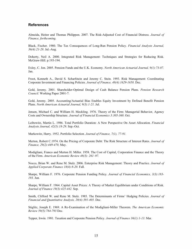
The common thread in the literature is the observation that there is a convex penalty for risk

which may be estimated ex-ante so that a decision may be made whether or not to hedge. The risk

penalty illustrated in Figure 1 is a function of possible variations in project outcomes. For

convenience, I have shown a zero penalty for project outcomes that meet or exceed

expectations.12

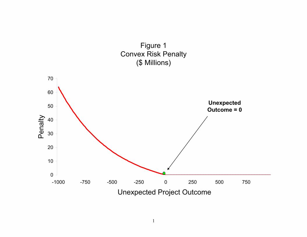
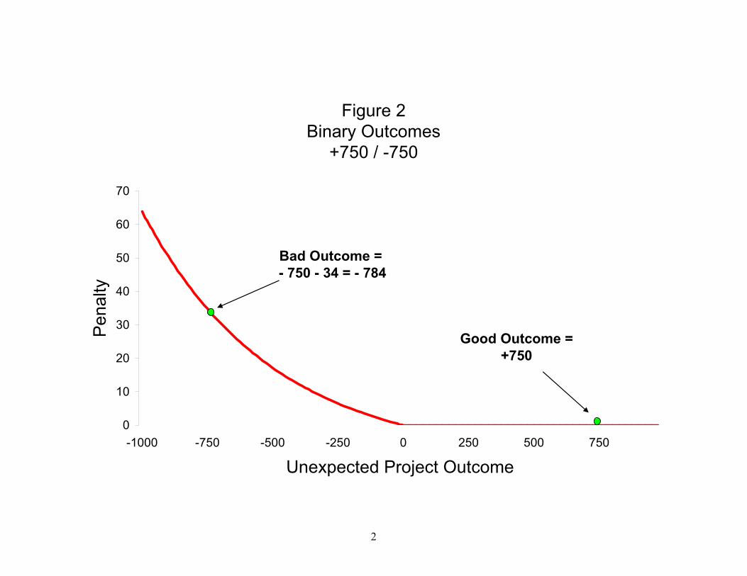
Suppose, as shown in Figure 2, that there are two equally likely outcomes with ex-ante values

$750 million above and below expected. If the inferior result occurs, we estimate $34 million in

secondary cost attributable to the causes outlined in the literature. One interpretation would be

that financial distress reduces franchise value by this ex-ante amount. Under these circumstances,

the expected financial distress cost is $17 million, as shown in Figure 3.

3.323 Hedging

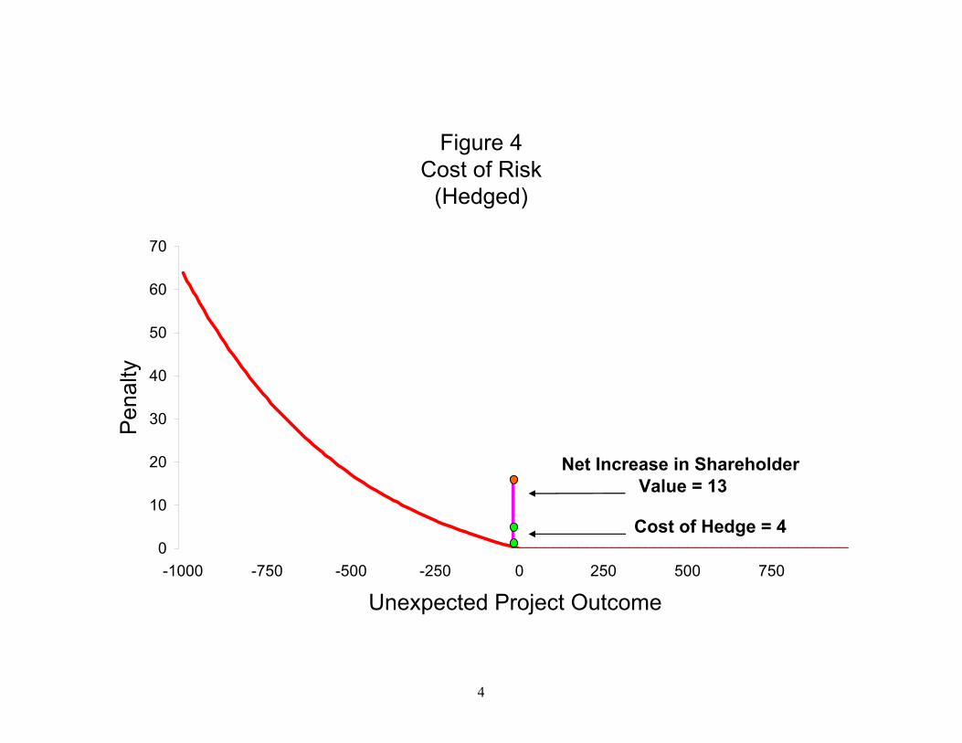
We next suppose, Figure 4, that a hedge may be effected at a cost of $4 million which will

eliminate the plus or minus $750 million uncertainty and thus the potential $34 million risk

penalty. The decision to hedge adds $13 million in shareholder value. Thus, by reducing level two

costs, risk management adds value that is independent of risk preferences or tolerances.

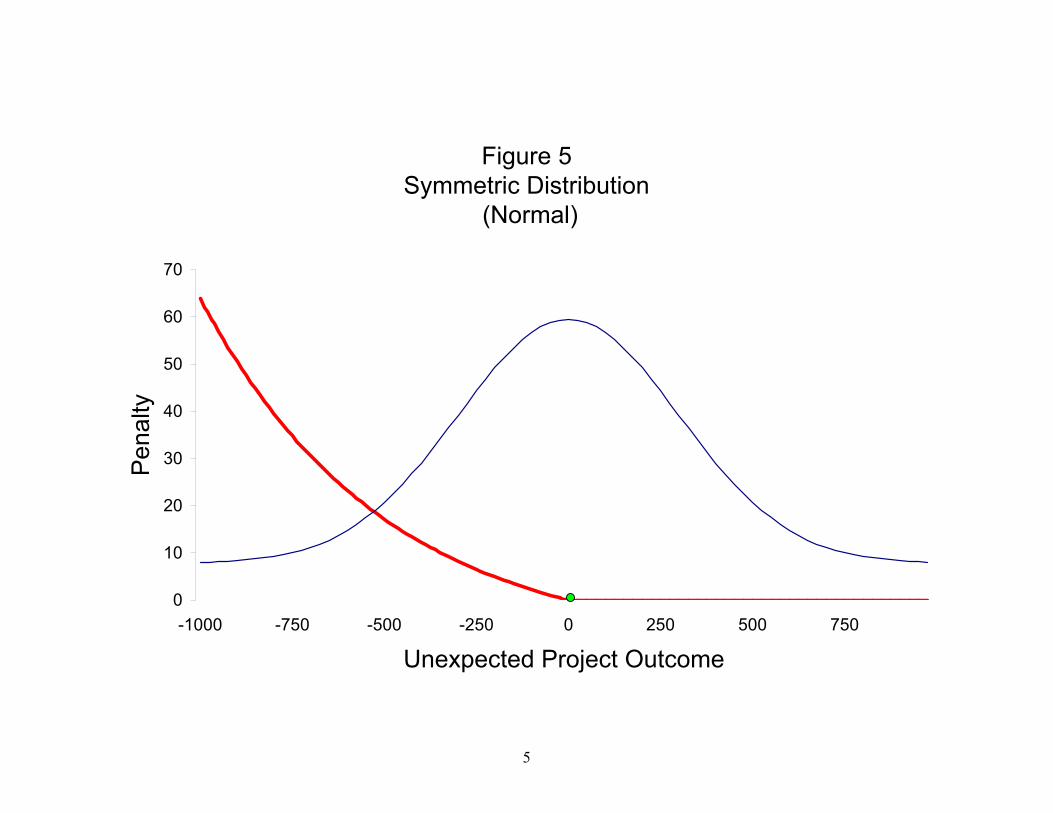
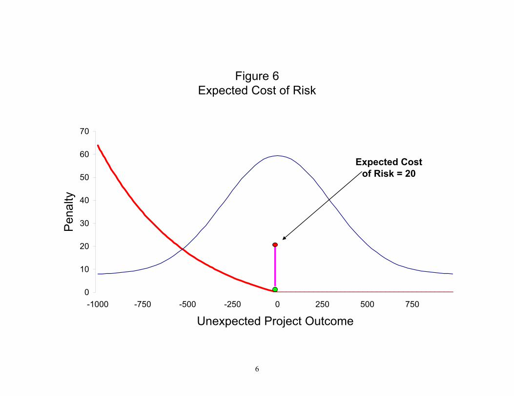
In Figure 5, we suppose a project-outcome distribution that is normal, rather than binary. From

now on we will integrate, rather than sum, in order to compute the expected risk penalty.13 In

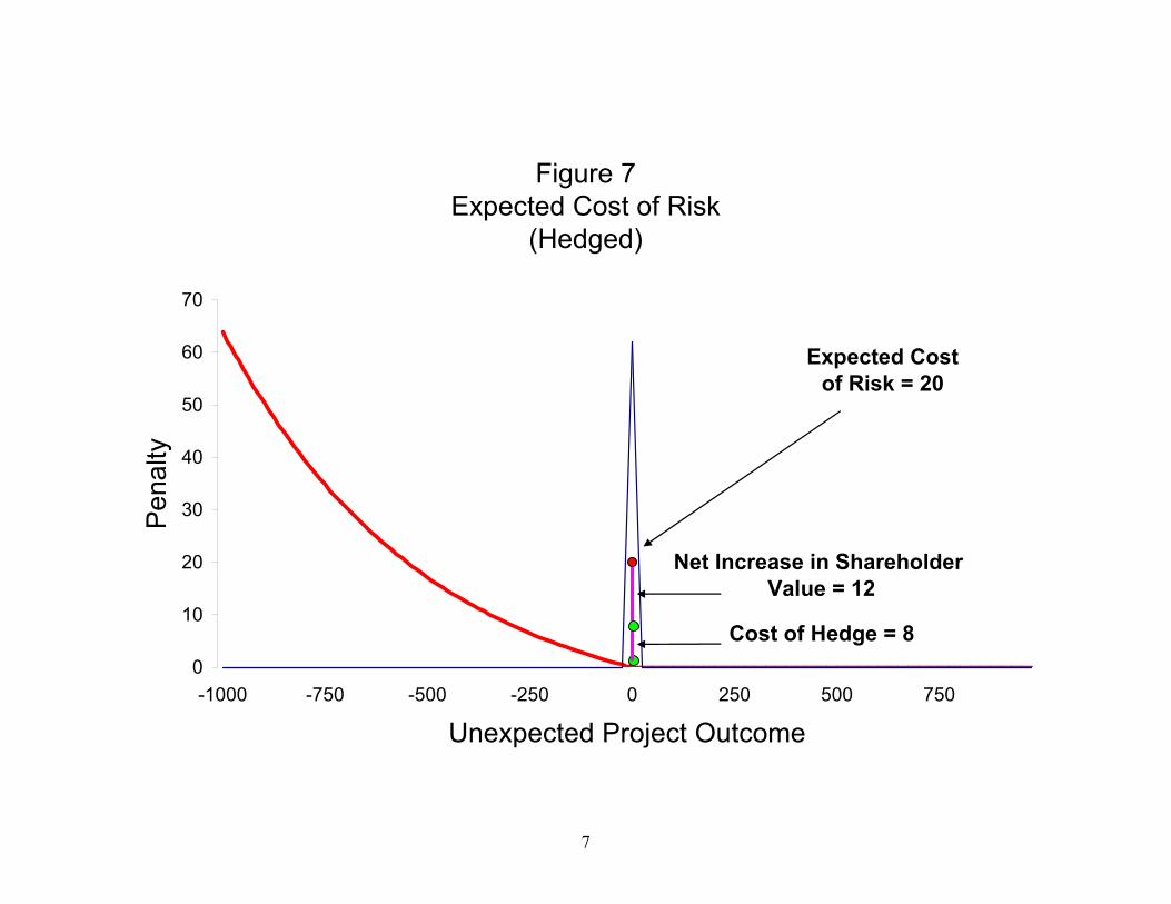
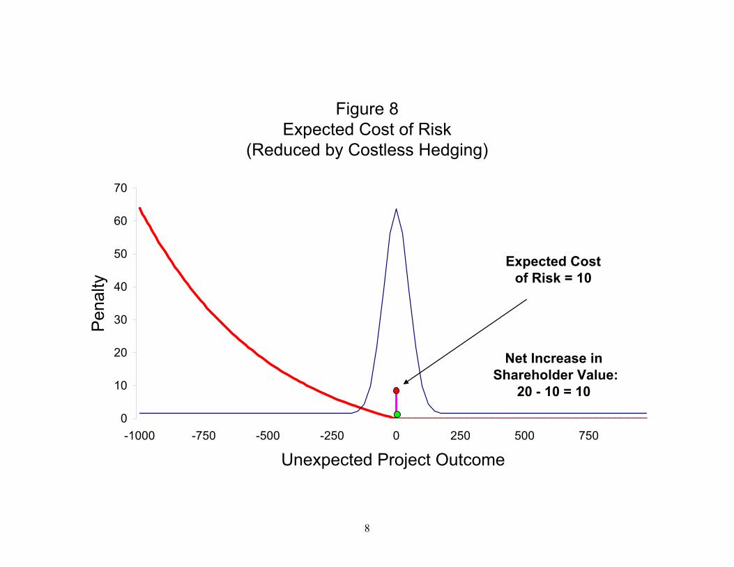
Figure 6, we suppose that the expected penalty is $20 million. If, as illustrated in Figure 7, we can

find hedges that sharply lower the distribution variance, we will be able to reduce the level two

cost by more than the cost of the hedge, thus generating shareholder value.

12 The penalty value for the expected outcome could be positive or negative and the curve need not be

linear at any point. The only necessary quality of the penalty is its convexity. 13 This suggests further research into the combination of risk penalty shapes and outcome distributions

that result in positive and negative level two costs.

10

Many of the uncertainties in project outcomes may depend on variables for which market hedges

exist: interest rates, energy and other commodity prices, foreign exchange rates, and general

equity exposure (β). Hedging transactions in these variables can usually be implemented at very

low cost – which in Figure 8 we will treat as cost free. Only the most efficient market hedges

come close to this ideal.14

4. Shorting the Market

The cheap hedges discussed above have generally been aimed at well-defined narrow exposures

such as interest rates, energy and currency. For such narrow exposures, the relationship between

the hedging instrument and the exposure will be quite tight and the hedges will contract the range

of project outcomes.

The goal, however, is ex-ante reduction of the variance of project outcomes and therefore a

broader hedge with the same statistical implication can be just as effective at increasing investor

value. Most publicly traded companies engage in projects whose outcomes correlate positively

with states of the world as represented by broad market indices; in short, their projects have

positive β. It is this property that underlies the observation by Almeida and Philippon (2007) that

financial distress has negative β – it is inherited from the positive project β of the company.

Suppose we hedge our project β15. We wish to determine how much to hedge when project

outcomes, with an ex-ante investment value of $1 million, are normally distributed with variance 2pσ and β equal to b. We will hedge this portfolio by shorting $c million of the market

portfolio.16 We are looking for the value of c that will minimize the variance of the firm’s hedged

project portfolio, where::

2p

uhVar σ=

mppmmph ccVar σσρσσ 2222 −+=

p

mpm b

σσρ =

14 Insurances and private contracts will be less efficient. Asymmetric insurances and options may also

change the distribution providing shareholder gains in exchange for premiums. Under the Smith and Stulz (1985) tax model, this may introduce additional costs.

15 We will hedge the residual β after narrower hedges have been implemented. 16 This may be implemented using various tools such as swaps and futures contracts.

11

2222 2 mmph cbcVar σσσ −+=

22 22 mm

h

bcc

Var σσ −=∂

∂

02 22

2

>=∂

∂m

h

cVar σ

bcc

Varh

=⇒=∂

∂ 0

where uhVar and hVar represent the project variance without and with hedging; 2mσ is the

variance of the market portfolio; and pmρ is the correlation coefficient between the project and

market portfolios. The positive second derivative indicates that we have minimized variance and

the final implication is that this is achieved when project β is fully hedged.

Notice that β need not be positive for optimal hedging. For the rare firm with negative project β, c

will be negative and the firm will implement its hedge by buying rather than shorting the market

portfolio.

Shareholders may adjust their portfolios to restore expected returns and risk by taking the

opposite hedge position, generally by buying the market portfolio. The net gain for shareholders

will then be measured by the reduction in deadweight (level two) financial distress cost.

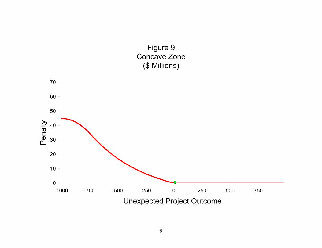
4.1 The Concave Zone

Figure 9 differs from Figure 1 for unexpected project losses greater than $750 million. Figure 9

reflects a limit on the convexity that can be postulated for the risk penalty of a limited liability

corporation. At some point bad project outcomes consume all the value (tangible and intangible)

held by the corporation. Although a firm financed entirely by equity investors might destroy all of

its value along a convex curve, it is more realistic to assume that diminishing franchise value and

a sharing of damage with other parties (lenders, guarantors, suppliers, etc.) will create a concave

penalty zone as shown on the left side of Figure 9.

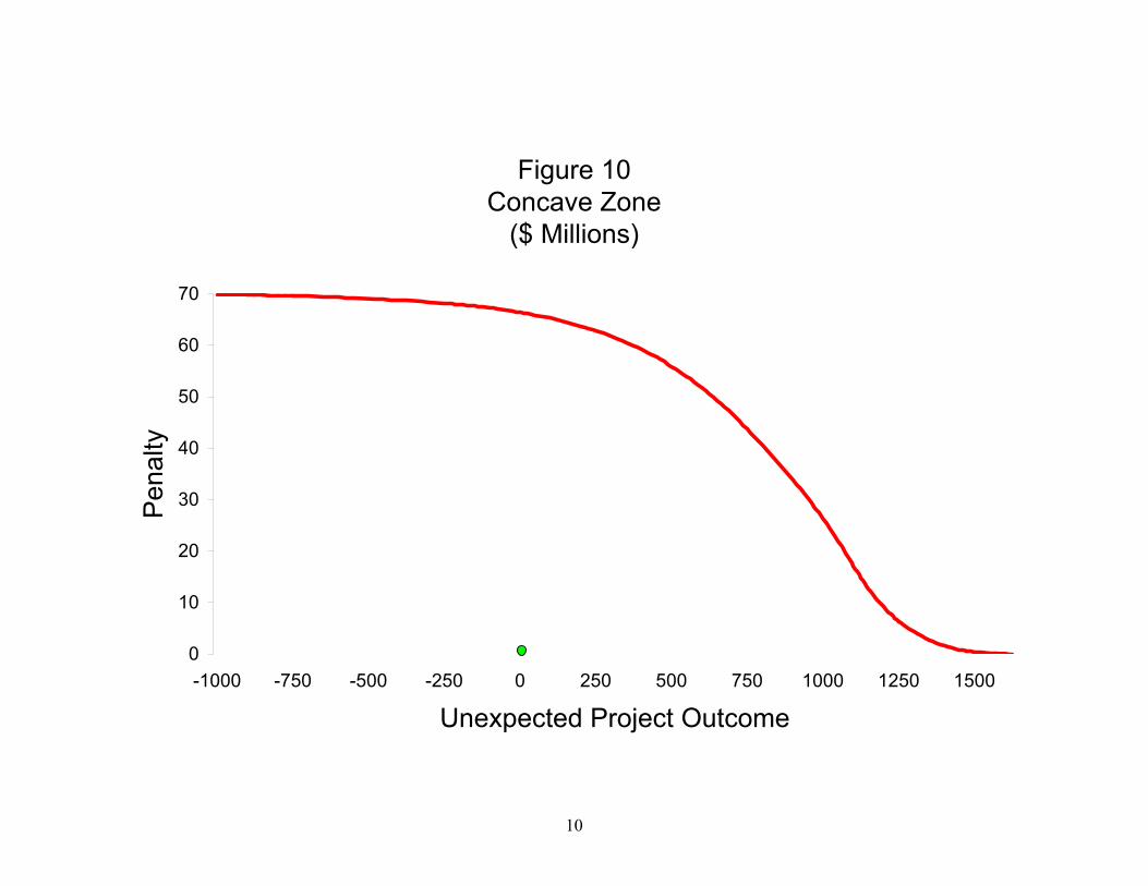
This shape is consistent with models of approaching bankruptcy (e.g., Merton 1974) where

control remains with shareholders whose ownership interest becomes manifestly option-like.

Sharpe (1976) identifies a similar optionality in the context of defined benefit plans guaranteed by

12

the U.S. Pension Benefit Guaranty Corporation (PBGC). A company whose forward prospects

are dire may find that the bulk of its likely project outcomes will fall in the concave zone as

shown in Figure 10.

Such companies increase shareholder value by increasing the riskiness of their underlying

projects – playing a “heads our shareholders win tails somebody else loses” game. For these

companies, prospective level two costs have become negative. Such companies might be advised

to forego hedging and take every gamble. It is interesting to note that one very solid U.S. airline

has hedged its fuel costs in recent years while its more troubled sisters have generally taken their

chances.

4.2 The Pension Gambit

Using common assumptions about transparency and investor diversification and rationality,

Tepper (1981) and Black (1980) show that investor value increases when corporate defined

benefit plans sell equities and buy bonds. They rely on tax rules in many countries where: 1) bond

returns are more highly taxed than stock returns in taxable accounts, and 2) special tax rules treat

pension plan stock and bond returns identically. Using Modigliani-Miller style arguments and

taking advantage of this differential tax treatment, they conclude that shareholders (Tepper) or the

corporations themselves (Black) can reproduce the investment risk (β) and expected equity

premiums while reducing taxes in their own accounts.

Twenty five years after publication, the lessons of Tepper and Black have yet to achieve

significant traction with practitioners. The emergence of LDI and impending changes to plan

accounting rules suggest that the future may be different from the past. Gold (2005) argues that

the prevailing accounting treatment17 creates spurious financial reporting benefits from equity

investments that stand as a barrier to economic value maximization via β reduction.

When the liabilities of the plans are modeled as zero-β cash flows, Tepper and Black maximize

value and minimize mismatch risk by setting pension asset β to zero. Gold (2001) extends Tepper

and Black in a model where the sponsor choose the asset β and defines the liability β, each in the

range [0,1]. Under these circumstances, shareholder value is maximized when asset β equals zero

and liability β equals one. There is nothing magic about the [0,1] limitation and level one value

17 FAS 87 in the US, CICA 3461 in Canada, FRS 17 in the UK, and IAS 19 internationally credit

immediate earnings for expected returns on risky assets, smoothing actual return deviations over time.

13

continues to grow as the net (asset minus liability) β decreases. But any non-zero net β indicates

mismatch risk and we have seen that risk can cause level two costs.

For the great majority of companies that have positive β project portfolios, we have seen that

shorting β actually reduces level two cost. Gold (2001) then implies that such firms should not

only hedge away their project β but should do so by establishing a net negative pension β

position. This layers two sources of economic value enhancement on top of each other. Overall

risk reduction lowers level two cost and the net negative β in the pension plan adds tax benefits.

Those companies with negative project β cannot achieve this double benefit and should acquire

their long β hedges on their balance sheets.

4.21 The Concave Pension Gambit

A company in the concave zone can take risks, including β, almost anywhere but we can identify

two reasons why the pension plan may be a good location: 1) the “independence” of the pension

plan may limit the ability of the sponsor’s creditors to invoke leverage-limiting covenants; and 2)

plan losses may be borne by guarantors such as the U.S. PBGC and the U.K. Pension Protection

Fund (PPF).

5. Conclusions

The corporate finance approach to risk management identifies a convex penalty that derives from

the common exceptions to the perfect markets of Modigliani and Miller (1958). This leads to

hedging activities that reduce the variation of project outcomes, increasing investor value by

lowering deadweight costs. The literature has not appeared to notice that hedging systematic risk

can similarly narrow the distribution of project outcomes. This paper argues that such hedging

can increases investor value.

Pension risk management has typically been addressed in an environment where taking market

risk to generate expected returns has been assumed to add value. Thus risk reduction has

generally been perceived as a restriction to this return seeking activity. The potential to add value

by eliminating market risk, identified twenty-five years ago by Tepper (1981) and Black (1980),

has not been widely embraced. Recent concerns about pension risk have revived some interest in

their work, but little action. This paper argues for an extension of Tepper and Black to establish

net negative market exposures in defined benefit pension plans under tax regimes common in

Anglo-Saxon nations.

14

Hedging systematic risk increases investor value and using defined benefit pension plans to do so

can add a second layer of value. The reluctance of defined benefit plan sponsors to reduce equity

exposure is strong and persistent. For numerous reasons, plan sponsors are exceedingly unlikely

to follow this course. It is therefore presumptuous of me to point out that an interesting piece of

follow up research might begin with the equilibrium question: what if every sponsor wanted to

short their own market exposure? Who would hold systematic risk and what equity risk premium

would be required?

15

References

Almeida, Heitor and Thomas Philippon. 2007. The Risk-Adjusted Cost of Financial Distress. Journal of Finance, forthcoming.

Black, Fischer. 1980. The Tax Consequences of Long-Run Pension Policy. Financial Analysts Journal, 36(4):21-28. Jul.-Aug.

Doherty, Neil A. 2000. Integrated Risk Management: Techniques and Strategies for Reducing Risk. McGraw-Hill. p.193-194.

Exley, C. Jon. 2005. Pension Funds and the U.K. Economy. North American Actuarial Journal, 9(1):73-87. Jan.

Froot, Kenneth A., David S. Scharfstein and Jeremy C. Stein. 1993. Risk Management: Coordinating Corporate Investment and Financing Policies. Journal of Finance, 48(4):1629-1658. Dec.

Gold, Jeremy. 2001. Shareholder-Optimal Design of Cash Balance Pension Plans. Pension Research Council. Working Paper 2001-7.

Gold, Jeremy. 2005. Accounting/Actuarial Bias Enables Equity Investment by Defined Benefit Pension Plans. North American Actuarial Journal, 9(3):1-21. Jul.

Jensen, Michael C. and William H. Meckling. 1976. Theory of the Firm: Managerial Behavior, Agency Costs and Ownership Structure. Journal of Financial Economics 3:305-360. Oct.

Leibowitz, Martin L. 1986. Total Portfolio Duration: A New Perspective On Asset Allocation. Financial Analysts Journal, 42(5):18-29. Sep.-Oct.

Markowitz, Harry. 1952. Portfolio Selection. Journal of Finance, 7(1), 77-91.

Merton, Robert C.1974. On the Pricing of Corporate Debt: The Risk Structure of Interest Rates. Journal of Finance, 29(2):449-470, May.

Modigliani, Franco and Merton H. Miller. 1958. The Cost of Capital, Corporation Finance and the Theory of the Firm. American Economic Review 48(3): 261–97.

Nocco, Brian W. and Rene M. Stulz. 2006. Enterprise Risk Management: Theory and Practice. Journal of Applied Corporate Finance 18(4):8-20. Fall.

Sharpe, William F. 1976. Corporate Pension Funding Policy. Journal of Financial Economics, 3(3):183-193. Jun.

Sharpe, William F. 1964. Capital Asset Prices: A Theory of Market Equilibrium under Conditions of Risk. Journal of Finance 19(3):425-442. Sep.

Smith, Clifford W. and Rene M. Stulz. 1985. The Determinants of Firms’ Hedging Policies. Journal of Financial and Quantitative Analysis, 20(4):391-405. Dec.

Stiglitz, Joseph E. 1969. A Re-Examination of the Modigliani-Miller Theorem. The American Economic Review 59(5):784-793 Dec.

Tepper, Irwin. 1981. Taxation and Corporate Pension Policy. Journal of Finance 36(1):1-13. Mar.

1

Figure 1Convex Risk Penalty

($ Millions)

0

10

20

30

40

50

60

70

-1000 -750 -500 -250 0 250 500 750

Unexpected Project Outcome

Pen

alty

Unexpected Outcome = 0

2

Figure 2Binary Outcomes

+750 / -750

0

10

20

30

40

50

60

70

-1000 -750 -500 -250 0 250 500 750


Pen

alty

Bad Outcome =- 750 - 34 = - 784

Good Outcome =+750

3

Figure 3Cost of Risk

0

10

20

30

40

50

60

70

-1000 -750 -500 -250 0 250 500 750


Pen

alty Expected Penalty = 17

Incremental Cost of Risk = 17

4

Figure 4Cost of Risk

(Hedged)

0

10

20

30

40

50

60

70

-1000 -750 -500 -250 0 250 500 750


Pen

alty

Net Increase in Shareholder Value = 13

Cost of Hedge = 4

5

Figure 5Symmetric Distribution

(Normal)

0

10

20

30

40

50

60

70

-1000 -750 -500 -250 0 250 500 750


Pen

alty

6

Figure 6Expected Cost of Risk

0

10

20

30

40

50

60

70

-1000 -750 -500 -250 0 250 500 750


Pen

alty

Expected Costof Risk = 20

7


(Hedged)

0

10

20

30

40

50

60

70

-1000 -750 -500 -250 0 250 500 750


Pen

alty

Cost of Hedge = 8

Net Increase in Shareholder Value = 12


8


(Reduced by Costless Hedging)

0

10

20

30

40

50

60

70

-1000 -750 -500 -250 0 250 500 750


Pen

alty

Net Increase in Shareholder Value:

20 - 10 = 10


9

Figure 9Concave Zone

($ Millions)

0

10

20

30

40

50

60

70

-1000 -750 -500 -250 0 250 500 750


Pen

alty

10

Figure 10Concave Zone

($ Millions)

0

10

20

30

40

50

60

70

-1000 -750 -500 -250 0 250 500 750 1000 1250 1500


Pen

alty

The Intersection of Pensions and Enterprise Risk Management...

Documents

Transcript of The Intersection of Pensions and Enterprise Risk Management...