The international mobility of highly educated …unctad.org/en/docs/iteiit20081a2_en.pdfThe...

The international mobility of highly

educated workers among OECD

countries*1

Steven Globerman and Daniel Shapiro**2

In this study, we specify and estimate an augmented gravity model of theIn this study, we specify and estimate an augmented gravity model of thedeterminants of bilateral migration flows across OECD countries. Our determinants of bilateral migration flows across OECD countries. Our specific focus is on the migration of highly educated workers (HEWs),specific focus is on the migration of highly educated workers (HEWs),and the impact on migration of bilateral trade and foreign direct and the impact on migration of bilateral trade and foreign direct investment (FDI). We argue that transnational corporations are efficient,investment (FDI). We argue that transnational corporations are efficient,direct channels for the movement of HEWs across international borders.direct channels for the movement of HEWs across international borders.Our results confirm the importance of FDI and trade as determinants of Our results confirm the importance of FDI and trade as determinants of migration flows: both are complements to migration. We also find that migration flows: both are complements to migration. We also find that migration of HEWs is greater between countries with large populationsmigration of HEWs is greater between countries with large populationsand less when geographic, linguistic and religious “distances” areand less when geographic, linguistic and religious “distances” arerelatively large. Migration is also influenced by labour market conditions.relatively large. Migration is also influenced by labour market conditions.Specifically, migrants tend to leave countries where economic conditionsSpecifically, migrants tend to leave countries where economic conditionsare relatively poor (high unemployment; low GDP per capita) and moveare relatively poor (high unemployment; low GDP per capita) and moveto areas where conditions are better. Finally, the results indicate that thereto areas where conditions are better. Finally, the results indicate that thereare important differences in the determinants of migration outcomes byare important differences in the determinants of migration outcomes bylevel of education. In particular, we find evidence that bilateral tradelevel of education. In particular, we find evidence that bilateral tradeand FDI have a greater impact on the migration of HEWs. In addition,and FDI have a greater impact on the migration of HEWs. In addition,highly educated migrants are more influenced by the “pull” of economichighly educated migrants are more influenced by the “pull” of economicconditions in host countries, while those with less education are moreconditions in host countries, while those with less education are moreheavily influenced by the “push” of economic factors in their homeheavily influenced by the “push” of economic factors in their homecountries.countries.

JEL Classification: F2, J6

Key words: migration, highly educated workers, globalization, gravitymodel.

1. Introduction

While the forces of globalization that have increased flows of goodsand capital also appear to have facilitated the international mobility of highly

1* The authors acknowledge funding from Industry Canada for this study. DanielBoothby provided helpful comments on an earlier draft. The comments and suggestions of threeanonymous reviewers are also gratefully acknowledged.

2** Steven Globerman is at Western Washington University, College of Business and Economics, Bellingham, Washington 98225. Email: [email protected]. DanielShapiro (corresponding author) is at Segal Graduate School of Business, Simon Fraser University, 515 West Hastings Street, Vancouver, B.C., Canada. Email: [email protected]

2 Transnational Corporations, Vol. 17, No. 1 (April 2008)

educated and skilled workers (Lopes, 2004; Docquier and Lodigiani,2007), the precise determinants of the international flows of suchworkers are not yet clear, in part because consistent internationaldata on the migration patterns of highly educated workers (HEWs)have been unavailable until recently. Therefore, although there is asubstantial literature on migration, both within and between nations(recent examples include Pedersen et al., 2004; Gonzalez and Maloney,2005; Mayda, 2005; Peri, 2005; Docquier and Marfouk 2006), there arerelatively few studies that focus specifically on HEWs.1 As a result, thereis a substantial amount of theorizing about the determinants of HEW migration with relatively limited accompanying empirical evidence. Inparticular, there is limited evidence regarding the impact of trade and foreign direct investment (FDI) on the international flows of HEWs.

The primary purpose of this study is to specify and estimate amodel of international migration using relatively recent OECD datathat distinguish migrants by education levels and country of origin. We employ a gravity model specification to estimate the determinants of bilateral migration among OECD countries using data for both sendingand receiving countries, while focusing particularly on the impact of bilateral movements of trade and FDI. We also add explanatory variablesthat account for cross-county differences in economic, geographic and cultural “distance”. The model is estimated for both HEWs and other migrants in order to identify what might be unique about the impact of trade and FDI on HEW migration.2

It can be argued that transnational corporations (TNCs) are efficient,direct channels for the movement of HEWs across international borders.Specifically, the internal labour markets of TNCs can be used to re-locatepeople across international borders, particularly HEWs with knowledgeor skills that can be efficiently shared across the locations in which theTNC operates. For example, Mahroum (1999) notes that the migration of managers and executives often originates with temporary intra-corporatetransfers that, later, turn into longer term, or even permanent moves. Thus,the extent of bilateral FDI can have a potentially important influence onbilateral migration flows. To the extent that TNCs use internal labour

1 For relatively recent studies, see Peri (2005) and Docquier and Marfouk (2006).2 It should be noted explicitly that the OECD data identify migrants, and not

more accurately potential workers. While it seems reasonable to conclude that most highly educated migrants obtain employment in host country labour markets, the foregoing distinction should be borne in mind. Nevertheless, for convenience, we may occasionally refer to highly educated “workers” rather than the more precise highlyeducated “individuals”.

Transnational Corporations, Vol. 17, No. 1 (April 2008) 3

markets to reallocate managers and technical personnel who are resident in different countries across transnational production units around theworld, FDI and the migration of HEWs will be complements.3 Docquier and Lodigiani (2007) find evidence of such complementarity in that theemigration of skilled migrants appears to encourage future inflows of FDI to the home countries. Using United States Census data, Kugler and Rapoport (2007) find that skilled migration and FDI inflows arenegatively correlated contemporaneously, but past skilled migration isassociated with an increase in current FDI inflows. Buch et al. (2003)find a relatively strong link between the stocks of German migrantsand the stocks of FDI abroad but the link between the immigration of foreigners to Germany and FDI inflows is weaker. Aroca and Maloney(2004), on the other hand, find that FDI and labour flows are substitutesin the case of Mexico. Hence, there is no strong consensus on whether FDI and labour flows are complements or substitutes and there are veryfew studies of the empirical linkage between FDI and the migration of HEWs specifically.4

At a general level, both the migration of HEWs and FDI flowsrepresent movement across borders of relatively mobile factors of production that are directly or indirectly human capital intensive. Factorsthat conceptually influence the migration decisions of HEWs are similar in many cases to those that conceptually influence FDI movements,particularly the degree of economic and social development of sendingand receiving countries, and the sizes of the sending and receivingcountries’ economies. In theory, FDI and international migration might be substitutes or complements, and the relationship could be different for HEWs and other migrants (Kugler and Rapaport, 2007). FDI and migration might be substitutes, for example, if FDI results in migrant workers in the home country being displaced by local workers in thehost country. Alternatively, FDI and the migration of HEWs might benet complements if TNCs use internal labour markets to reallocatemanagers and technical personnel who are resident in different countriesacross transnational production units around the world.

Similarly, trade and migration are likely to be linked directly.The efficient exploitation of information about trade opportunities and key success factors in importing and exporting activities may requirethe physical movement of HEWs across countries. Effectively, labour

3 An offsetting factor might be noted. If FDI increases real wages in the host country, outbound migration might be reduced at the margin.

4


mobility is an instrument for diffusing information about geographicallysegmented markets (Combes et al., 2005). At the same time, FDI isindirectly linked to the migration of HEWs through the relationshipbetween trade and FDI. A substantial share of international trade takesthe form of intra-firm trade carried out by TNCs, and for that reasontrade and FDI tend to be complements (Globerman and Shapiro, 2002).The implication for models of HEW migration is that trade-creating FDIcan be expected to encourage HEW migration flows.5

In sum, we suggest that a key input to the efficient operation of TNC global networks is the effective diffusion of information and skillswithin the TNC that requires substantial intra-corporate transfers of HEWs among TNC affiliates. These transfers create a complementaryrelationship between the mobility of HEWs and both FDI and tradeflows.

In fact, a key empirical finding of our study is that HEW migration is strongly complementary to FDI and trade flows suggestingthat the migration of HEWs is increasingly an aspect of the global production systems created and operated primarily by TNCs. We alsofind that while local economic conditions in the home and host countriesare important determinants of migration for individuals at all levelsof attained education, the “pull” factor of host country conditions isapparently more significant the higher the individual’s formal educationlevel. Both physical and cultural distances between host and home countries influence migration, although not identically across different levels of education.

The remainder of the article proceeds as follows. Although it is somewhat unusual to begin with a discussion of data, we do so insection 2, where we describe the OECD migration data employed in our empirical analysis. The data report stocks of immigrants and emigrants for 29 OECD countries. Immigration and emigration data are reported for three categories of educational attainment. The stock data thereforereflect the cumulative flow of both permanent and temporary potentialworkers at different educational levels over past decades, as reflected in2000 Census data or equivalent sources.

5 The potential for the participation of migrants in trade networks to increase tradeby reducing transaction and other types of information costs is discussed by Gould (1994), Rauch and Trindade (2002) and Docquier and Lodigiani (2007), among others; however,


Section 3 presents a simple model of international migrationdecisions which we use to derive an equation to be estimated, based onthe gravity model. In the gravity equation, the logarithm of the number of foreign born persons in any one country that originate in a second OECD country are regressed on a number of variables that measurecharacteristics of both countries. Section 4 discusses the specificationof that equation, mainly with respect to the choice of explanatoryvariables.

Section 5 presents and discusses the empirical results. Theresults suggest that the international migration of individuals is well-explained by a model that includes both economic and non-economic variables. As noted above, we find that bilateral movements of goodsand capital are positively related to bilateral movements of people.Thus, the globalization of economic relationships is important to our understanding of international migration. Although we expected theserelationships to be more important for HEWs, we find that they affect allinternational migration. Nevertheless, some differences exist betweenthe determinants of HEW migration and total migration. A summary of our findings is presented in section 6.

2. The OECD database

Our empirical analysis is based on recently published OECDdata on migration patterns for individuals possessing different levels of education.6 These data are collected in a uniform way, thereby addressingsome previous problems surrounding earlier studies of internationalmigration patterns. In particular, many countries previously reported data only for the number of foreign nationals, rather than the number of foreign-born. A focus only on foreign nationals is likely to understateconsiderably the number of immigrants (Dumont and Lemaitre, 2004).7

Moreover, it might distort comparisons across countries to the extent that the ratio of foreign nationals to total immigrants varies across

6 The underlying data are described in J.C. Dumont and G. Lemaitre (2004, 2005).Peri (2005) uses this data set for his empirical model of international migration. A similar database has been constructed by Docquier and Marfouk (2004, 2006). However,Docquier (2006, p. 5) reports a very high correlation between the Docquier-Marfouk and Dumont-Lemaître estimates of emigration rates by educational attainment (between .88and .91) for 2000.

7

country of birth may be especially problematic for some countries such as the CzechRepublic and Slovakia which used to be one country.


countries. The OECD database provides an internationally comparabledata set with detailed information on the foreign-born population of OECD countries, by country of origin and by level of education. Thus,this data set allows a reliable means to compare immigrant populationsacross countries and, importantly, to identify the migration patterns of HEWs.

The OECD data report stocks of immigrants and emigrants in 29OECD countries based on country of birth. For most countries, the datawere collected from population censuses or population registers that identified people by country of birth and level of education. In somecases, such as the Republic of Korea and Japan, where country of birthwas not available, nationality was used as a proxy measure for countryof birth. For most countries, the data are recorded as of 2000, and for most countries the data were obtained from population census for theyear 2000. For the 29 countries participating in the data collection, fairlydetailed data were obtained. The objective was to minimize the number of residual categories (“Other”). As a result, 227 OECD and non-OECDcountries and areas were identified as “countries of birth” for each of the29 OECD countries. By focusing on country of birth, the OECD dataprovide a more comprehensive measure of international migration thanearlier databases because they include all migrants, and not just thosewho are permanent residents. For the purposes of this study, we focuson the bilateral flows among OECD countries.8

The education and skill qualifications were based on theInternational Standard Classification of Education System (ISCED).Since data were unavailable for all countries on a sufficiently detailed basis, the ISCED system was used to create three broad categories of education: less than upper secondary (ISCED 0/1/2); upper secondaryand post-secondary non-tertiary (ISCED 3/4) and tertiary (ISCED 5/6).A residual category was also created for “unknown status”.

Evidently, creating the data involved a variety of judgments, including those regarding how to define countries.9 Perhaps the most important point to note is that the immigration data are stocks, not flows.The stock data therefore reflect the cumulative flow of permanent and temporary workers over past decades as reflected in 2000 Census dataor equivalent sources. It is likely that the stock of immigrants reported

8 We focus exclusively on OECD countries because reliable data on bilateral FDI

9 Many of these issues are discussed more fully in Dumont and Lemaitre (2004).


in 2000 census migrated in the 1980s and, particularly, in the 1990s.For one thing, a substantial percentage of immigrants who migrated in earlier decades are likely to be deceased. For another, temporary immigration based upon work-related visas was substantially greater in the 1990s than in earlier decades. The implication is that the most relevant determinants of the immigrant stocks reported in the OECDdatabase are likely to reflect economic and other conditions prevalent inthe 1980s and 1990s, rather than much earlier periods.

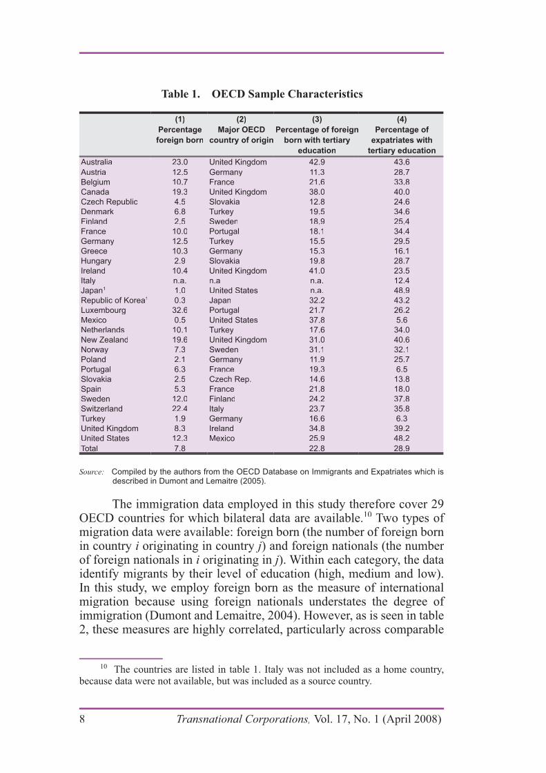
Table 1 provides a summary of some elements of the data.Specifically, it reports the percentage of foreign born, the major OECD country of origin for foreign born, the percentage of foreign-born immigrants possessing a tertiary education and the percentage of expatriates possessing a tertiary education. As can be seen in column 1 of table 1, there is considerable variation across countries in the percentageof foreign-born with the “settlement” countries of Australia, Canadaand New Zealand having foreign-born populations as a share of totalpopulation well above the OECD mean. It is also seen that Luxembourgand Switzerland have foreign-born populations that exceed 20 percent of total population, while some European countries, including Austria,Germany and the Netherlands, have percentages that exceed that for theUnited States. As noted by Dumont and Lemaitre (2004), the percentagesreported in column 1 are appreciably higher than those obtained whenimmigration is measured on the basis of foreign-born nationals, and thisis particularly true for Europe.

The immigrants originated from over 200 counties and areas, but in this study we focus only on OECD countries of origin. Column 2identifies the most prominent OECD country of origin for each of theOECD countries in the sample. For the most part, these are also thelargest source countries in general, e.g. the United Kingdom It can alsobe seen that the largest source country is often characterized by former colonial ties, (the United Kingdom is the largest source country for Australia, Canada and New Zealand), by contiguous borders (Germanywith Austria and Poland), or by previous history (Czech Republic and Slovakia; the United Kingdom and Ireland). In addition, the importanceof Turkish immigrants, often as guest workers, across Europe is clearlyevident. Columns 3 and 4 illustrate the propensity of the highly educated to migrate. Specifically, the mean percentage of foreign-born with atertiary education is well above the population means for the samplecountries, as is the percentage of expatriates with a tertiary education.


Table 1. OECD Sample Characteristics

(1)

Percentage

foreign born

(2)

Major OECD

country of origin

(3)

Percentage of foreign

born with tertiary

education

(4)

Percentage of

expatriates with

tertiary education

AustraliaAustralia 23.023.0 United KingdomUnited Kingdom 42.942.9 43.643.6

AustriaAustria 12.512.5 GermanyGermany 11.311.3 28.728.7

BelgiumBelgium 10.710.7 FranceFrance 21.621.6 33.833.8

CanadaCanada 19.319.3 United KingdomUnited Kingdom 38.038.0 40.040.0

Czech RepublicCzech Republic 4.54.5 SlovakiaSlovakia 12.812.8 24.624.6

DenmarkDenmark 6.86.8 TurkeyTurkey 19.519.5 34.634.6

FinlandFinland 2.52.5 SwedenSweden 18.918.9 25.425.4

FranceFrance 10.010.0 PortugalPortugal 18.118.1 34.434.4

GermanyGermany 12.512.5 TurkeyTurkey 15.515.5 29.529.5

GreeceGreece 10.310.3 GermanyGermany 15.315.3 16.116.1

HungaryHungary 2.92.9 SlovakiaSlovakia 19.819.8 28.728.7

IrelandIreland 10.410.4 United KingdomUnited Kingdom 41.041.0 23.523.5

ItalyItaly n.a.n.a. n.an.a n.a.n.a. 12.412.4

JapanJapan11 1.01.0 United StatesUnited States n.a.n.a. 48.948.9

Republic of KoreaRepublic of Korea11 0.30.3 JapanJapan 32.232.2 43.243.2

LuxembourgLuxembourg 32.632.6 PortugalPortugal 21.721.7 26.226.2

MexicoMexico 0.50.5 United StatesUnited States 37.837.8 5.65.6

NetherlandsNetherlands 10.110.1 TurkeyTurkey 17.617.6 34.034.0

New ZealandNew Zealand 19.619.6 United KingdomUnited Kingdom 31.031.0 40.640.6

NorwayNorway 7.37.3 SwedenSweden 31.131.1 32.132.1

PolandPoland 2.12.1 GermanyGermany 11.911.9 25.725.7

PortugalPortugal 6.36.3 FranceFrance 19.319.3 6.56.5

SlovakiaSlovakia 2.52.5 Czech Rep.Czech Rep. 14.614.6 13.813.8

SpainSpain 5.35.3 FranceFrance 21.821.8 18.018.0

SwedenSweden 12.012.0 FinlandFinland 24.224.2 37.837.8

SwitzerlandSwitzerland 22.422.4 ItalyItaly 23.723.7 35.835.8

TurkeyTurkey 1.91.9 GermanyGermany 16.616.6 6.36.3

United KingdomUnited Kingdom 8.38.3 IrelandIreland 34.834.8 39.239.2

United StatesUnited States 12.312.3 MexicoMexico 25.925.9 48.248.2

TotalTotal 7.87.8 22.822.8 28.928.9

Source: Compiled by the authors from the OECD Database on Immigrants and Expatriates which isdescribed in Dumont and Lemaitre (2005).

The immigration data employed in this study therefore cover 29 OECD countries for which bilateral data are available.10 Two types of migration data were available: foreign born (the number of foreign bornin country i originating in country j) and foreign nationals (the number of foreign nationals in i originating in j). Within each category, the dataidentify migrants by their level of education (high, medium and low).In this study, we employ foreign born as the measure of internationalmigration because using foreign nationals understates the degree of immigration (Dumont and Lemaitre, 2004). However, as is seen in table2, these measures are highly correlated, particularly across comparable

10 The countries are listed in table 1. Italy was not included as a home country,because data were not available, but was included as a source country.


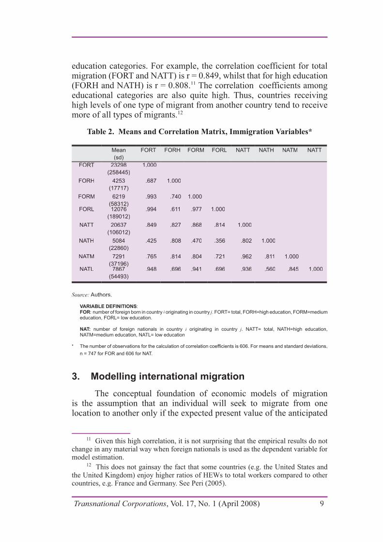
education categories. For example, the correlation coefficient for totalmigration (FORT and NATT) is r = 0.849, whilst that for high education(FORH and NATH) is r = 0.808.11 The correlation coefficients among educational categories are also quite high. Thus, countries receivinghigh levels of one type of migrant from another country tend to receivemore of all types of migrants.12

Table 2. Means and Correlation Matrix, Immigration Variables*

Mean

(sd)

FORT FORH FORM FORL NATT NATH NATM NATT

FORTFORT 2329823298

(258445)(258445)

1.0001.000

FORHFORH 42534253

(17717)(17717)

.687.687 1.0001.000

FORMFORM 62196219

(58312)(58312)

.993.993 .740.740 1.0001.000

FORLFORL 1207612076

(189012)(189012)

.994.994 .611.611 .977.977 1.0001.000

NATTNATT 2063720637

(106012)(106012)

.849.849 .827.827 .868.868 .814.814 1.0001.000

NATHNATH 50845084

(22860)(22860)

.425.425 .808.808 .470.470 .356.356 .802.802 1.0001.000

NATMNATM 72917291

(37196)(37196)

.765.765 .814.814 .804.804 .721.721 .962.962 .811.811 1.0001.000

NATLNATL 78677867

(54493)(54493)

.948.948 .696.696 .941.941 .696.696 .936.936 .560.560 .845.845 1.0001.000

Source: Authors.

VARIABLE DEFINITIONS:FOR: number of foreign born in country i originating in country j. FORT= total, FORH=high education, FORM=mediumeducation, FORL= low education.

NAT: number of foreign nationals in country i originating in country j. NATT= total, NATH=high education, NATM=medium education, NATL= low education

* The number of observations for the calculation of correlation coefficients is 606. For means and standard deviations,

n = 747 for FOR and 606 for NAT.

3. Modelling international migration

The conceptual foundation of economic models of migrationis the assumption that an individual will seek to migrate from onelocation to another only if the expected present value of the anticipated

11 Given this high correlation, it is not surprising that the empirical results do not change in any material way when foreign nationals is used as the dependent variable for model estimation.

12 This does not gainsay the fact that some countries (e.g. the United States and the United Kingdom) enjoy higher ratios of HEWs to total workers compared to other countries, e.g. France and Germany. See Peri (2005).


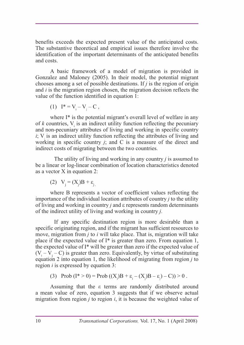
benefits exceeds the expected present value of the anticipated costs.The substantive theoretical and empirical issues therefore involve theidentification of the important determinants of the anticipated benefitsand costs.

A basic framework of a model of migration is provided in Gonzalez and Maloney (2005). In their model, the potential migrant chooses among a set of possible destinations. If jf is the region of origin jand i is the migration region chosen, the migration decision reflects thevalue of the function identified in equation 1:

(1) I* = Vi

V – Vj

V – C ,

where I* is the potential migrant’s overall level of welfare in anyof k countries, Vk

iV is an indirect utility function reflecting the pecuniary

and non-pecuniary attributes of living and working in specific countryi; V

jV is an indirect utility function reflecting the attributes of living and

working in specific countryjj

j; and C is a measure of the direct and indirect costs of migrating between the two countries.

The utility of living and working in any country j is assumed tojbe a linear or log-linear combination of location characteristics denoted as a vector X in equation 2:

(2) Vj

V = (Xj

X )B + j ,

where B represents a vector of coefficient values reflecting the importance of the individual location attributes of country j to the utility jof living and working in country j and represents random determinants of the indirect utility of living and working in country j.

If any specific destination region is more desirable than a specific originating region, and if the migrant has sufficient resources tomove, migration from j toj i will take place. That is, migration will takeplace if the expected value of I* is greater than zero. From equation 1,the expected value of I* will be greater than zero if the expected value of (V

iV – V

jV – C) is greater than zero. Equivalently, by virtue of substituting

equation 2 into equation 1, the likelihood of migrating from regionj

j tojregion i is expressed by equation 3:

(3) Prob (I* > 0) = Prob ((Xi)B +

i– (X

jX )B –

j) – C)) > 0 .

Assuming that the terms are randomly distributed around a mean value of zero, equation 3 suggests that if we observe actualmigration from region j to regionj i, it is because the weighted value of


the attributes of living and working in region i impart greater utility than the weighted value of the attributes of living and working in region j.13

That is, observed migration from j toj i (Mij) will be a function of

Xi, X

jX and C.

(4) Mij = f ( X

i, X

jX , C) .

The specification of a migration model therefore requiresspecifying the vectors X

i and X

jX for all sample countries, as well as the

precise functional form of the equation. We discuss the X-vectors in thej

next section, and here focus on functional form, for which we employ agravity model.

Gravity models have become the standard technique for theempirical analysis of inter-regional and international bilateral flowsof capital and goods. The basis of most empirical models of bilateraltrade and FDI flows is the “barebones” gravity equation, whereby anyinteraction between a pair of countries is modelled as an increasingfunction of their sizes and a decreasing function of the distance betweenthe two countries (Sen and Smith, 1995; Frankel and Rose, 2002).Indeed, the gravity equation has become “the workhorse for empiricalstudies….to the virtual exclusion of other approaches”, (Eichengren and Irwin, 1998, p. 13).14 While this statement was written with referenceto trade flows, the logic of the gravity model also underlies migrationstudies (recent examples include Karemera et al., 2000; Gonzalez and Maloney, 2005; Mayda, 2005; Peri, 2005) and FDI studies (Hejazi and Safarian, 2001; Hejazi and Pauly, 2005).

The underlying logic of applying the gravity model to migrationwas first set out by Zipf (1946). Clearly, the likelihood of an individualmigrating from any country should increase as the population of that country increases, holding other factors constant. Less obviously, thelikelihood of that individual migrating to any specific country should increase as the total population of the specific country increases, to theextent that potential receiving countries have implicit or explicit targets,or quotas, on allowable numbers of immigrants that, in turn, are functionsof total population of potential host countries.15

13 In a cross-section of paired countries, migration from region j to region iwould indicate that region i is preferable to all other possible regions for the relevant observations.

14 Frankel and Rose (2002) also note that the gravity equation as applied tointernational trade is one of the more successful empirical models in economics.

15 For additional discussion of how the supply and demand for migrants can be linked to the sizes of the sending and receiving countries, see Karemera et al. (2000).

Accordingly, we employ a gravity model specification suchthat bilateral flows from jm toj i are directly proportional to the “mass”of i and j, and inversely proportional to the “distance” between iand j, where distance can be interpreted to include geographic,cultural and economic distance. Thus, we estimate variations of equation 5:

(5) Mij = f ( (POP

ix POP

jP ), D

ij, L

ij, Z

ij) .

In the equation, Mij represents migration from country j to

country i; POP is the population of each country;ij

16 D is vector of terms representing measures of geographic and socio-culturaldistance between i and j; the L terms represent economic distancein terms of labour market differences (unemployment rates and average real wages); and the Z’s reflect other attributes of countriesi and j that might plausibly affect migration between the two countries.jIn our case, the Z vector includes measures of bilateral trade and FDI, as well as a dummy variable equal to unity when the United States is thereceiving country. These variables are discussed in the next section.

4. Model specification: independent variables

The dependent variables Mij

have been discussed above, and arebased on the OECD data. The full set of explanatory variables included

j

in the model, with their predicted impact on migration, is summarized in table 3, and the variables are more fully defined in table 4. Beforeconsidering each variable, three broad comments are in order.

First, although we have not to this point explicitly distinguished HEW migration from other migration, we do so in table 3. Althoughthe hypothesized direction of the impact of each explanatory variable isthe same for all types of migration, we suggest that the magnitude maydiffer. We will argue below that an important difference between HEW and other migration is likely to be linked to the trade and FDI variables.However, where relevant, we will also note other cases where the impact of a specific variable might be different for HEWs.

The latter suggest another possibility. Namely, that as more resources are diverted to agrowing home population, attractive opportunities available to migrants decline, therebydiscouraging migration to growing countries.

16 In migration models, it is typically population measures that serve as a measureof mass (Zipf, 1946; Gonzalez and Maloney, 2005). In trade and FDI models, GDP is more typically employed. Estimates replacing POP with GDP are similar to thosereported below.


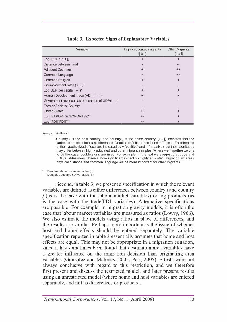
Table 3. Expected Signs of Explanatory Variables

Variable Highly educated migrants

(j to i)

Other Migrants

(j to i)

Log (POPi*POPj)Log (POPi*POPj) ++ ++

Distance between i and jDistance between i and j -- ----

Adjacent CountriesAdjacent Countries ++ ++++

Common LanguageCommon Language ++ ++++

Common ReligionCommon Religion ++ ++

Unemployment rates,( i – j)*Unemployment rates,( i – j)* -- --

Log GDP per capita,(i – j)*Log GDP per capita,(i – j)* ++ ++

Human Development Index (HDI),( i – j)*Human Development Index (HDI),( i – j)* ++ ++

Government revenues as percentage of GDP,(i – j)*Government revenues as percentage of GDP,(i – j)* -- --

Former Socialist CountryFormer Socialist Country -- --

United StatesUnited States ++++ ++

Log (EXPORTSij*EXPORTSji)**Log (EXPORTSij*EXPORTSji)** ++++ ++

Log (FDIij*FDIji)**Log (FDIij*FDIji)** ++++ ++

Source: Authors.

Country i is the host country, and country j is the home country. (i – j) indicates that the variables are calculated as differences. Detailed definitions are found in Table 4. The direction of the hypothesized effects are indicated by + (positive) and – (negative), but the magnitudesmay differ between highly educated and other migrant samples. Where we hypothesize this to be the case, double signs are used. For example, in the text we suggest that trade andFDI variables should have a more significant impact on highly educated migration, whereasphysical distance and common language will be more important for other migrants..

* Denotes labour market variables (L)** Denotes trade and FDI variables (Z)

Second, in table 3, we present a specification in which the relevant variables are defined as either differences between country i and countryj (as is the case with the labour market variables) or log products (asjis the case with the trade/FDI variables). Alternative specificationsare possible. For example, in migration gravity models, it is often thecase that labour market variables are measured as ratios (Lowry, 1966).We also estimate the models using ratios in place of differences, and the results are similar. Perhaps more important is the issue of whether host and home effects should be entered separately. The variablespecification reported in table 3 essentially assumes that home and host effects are equal. This may not be appropriate in a migration equation,since it has sometimes been found that destination area variables havea greater influence on the migration decision than originating areavariables (Gonzalez and Maloney, 2005; Peri, 2005). F-tests were not always conclusive with regard to this restriction, and we thereforefirst present and discuss the restricted model, and later present resultsusing an unrestricted model (where home and host variables are entered separately, and not as differences or products).


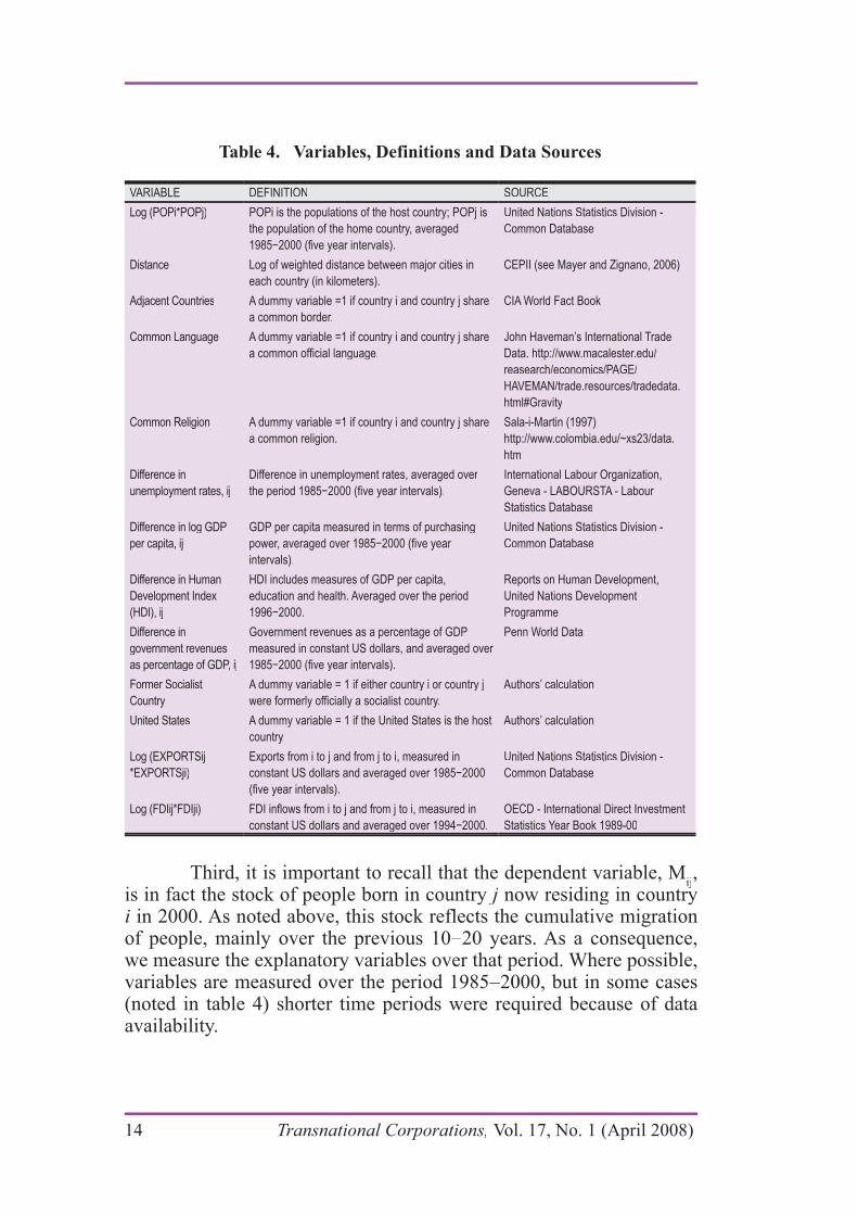
Third, it is important to recall that the dependent variable, Mij,

is in fact the stock of people born in country j now residing in countryj

ji in 2000. As noted above, this stock reflects the cumulative migrationof people, mainly over the previous 10 20 years. As a consequence,we measure the explanatory variables over that period. Where possible,variables are measured over the period 1985 2000, but in some cases (noted in table 4) shorter time periods were required because of dataavailability.

Table 4. Variables, Definitions and Data Sources

VARIABLE DEFINITION SOURCE

Log (POPi*POPj)Log (POPi*POPj) POPi is the populations of the host country; POPj isPOPi is the populations of the host country; POPj is

the population of the home country, averagedthe population of the home country, averaged

United Nations Statistics Division -United Nations Statistics Division -

Common DatabaseCommon Database

DistanceDistance Log of weighted distance between major cities inLog of weighted distance between major cities in

Adjacent CountriesAdjacent Countries A dummy variable =1 if country i and country j shareA dummy variable =1 if country i and country j share CIA World Fact Book CIA World Fact Book

Common LanguageCommon Language A dummy variable =1 if country i and country j shareA dummy variable =1 if country i and country j share John Haveman’s International TradeJohn Haveman’s International Trade

Common ReligionCommon Religion A dummy variable =1 if country i and country j shareA dummy variable =1 if country i and country j share Sala-i-Martin (1997)Sala-i-Martin (1997)

htmhtm

Difference inDifference in

unemployment rates, ijunemployment rates, ij

Difference in unemployment rates, averaged over Difference in unemployment rates, averaged over International Labour Organization, International Labour Organization,

Statistics DatabaseStatistics Database

per capita, ijper capita, ij



Difference in HumanDifference in Human

(HDI), ij(HDI), ij

Reports on Human Development,Reports on Human Development,

United Nations Development United Nations Development

ProgrammeProgramme

Difference inDifference in

government revenues government revenues measured in constant US dollars, and averaged over measured in constant US dollars, and averaged over

Penn World DataPenn World Data

Former Socialist Former Socialist

CountryCountry

A dummy variable = 1 if either country i or country j A dummy variable = 1 if either country i or country j Authors’ calculationAuthors’ calculation

United StatesUnited States A dummy variable = 1 if the United States is the hostA dummy variable = 1 if the United States is the host

countrycountry

Authors’ calculationAuthors’ calculation

Log (EXPORTSijLog (EXPORTSij

*EXPORTSji)*EXPORTSji)



Log (FDIij*FDIji)Log (FDIij*FDIji) FDI inflows from i to j and from j to i, measured inFDI inflows from i to j and from j to i, measured in OECD - International Direct InvestmentOECD - International Direct Investment


Most studies proxy migration costs using various measures of distance. Dostie and Leger (2004) suggest that the physical distancebetween origin and destination locations might be a good proxy for thecosts associated with migrating from one location to another. Gonzalezand Maloney (2005) link physical distance to moving costs but seenetworks of migrants from the same home country as an important factor influencing the costs directly or indirectly borne by immigrantsassociated with assimilating into the host country. Pedersen et al.(2004) and Mayda (2005) use dummy variables for countries that sharecommon borders and common languages as proxies for migration costs.Presumably, employment should be easier to secure when the migrant already possesses host country language skills; however, since HEWs aremore likely to have acquired other languages, a common language at thecountry level may be a less relevant determinant of HEW migration.17

We include four “distance”-related variables (physical distance,adjacent country, common language and common religion). Physicaldistance accounts for both transportation and communications costs.The expected effect on migration is negative, because the costs of acquiring information, communicating with potential employersand travelling between the originating and destination countries willincrease with physical distance. We suggest, however, that the impact of physical distance will be less for HEWs, who are both better able toafford the pecuniary costs associated with travel and have better accessto transaction-cost reducing means of communication and informationgathering (such as the Internet).18 For international migration, it is not obvious how to measure physical distances, since distances will also befunctions of location within countries. Accordingly, we use the weighted distance measure provided by CEPII as described in Mayer and Zignano(2006). In addition, however, we also include a dummy variable for geographic adjacency to account for the ease of movement across commonborders. Other things equal, adjacency should encourage migration. For similar reasons as above, we expect the effect of geographic adjacencyto be weaker for HEWs than for other migrants.

17 A number of authors have noted that foreign students enrolled in host country

costs normally associated with migration to that host country as an HEW in the future(Tremblay, 2004). In some cases, foreign students may retain their residency in the host country by converting their visa status upon obtaining permanent employment.

18 Arguably, physical distance, per se, should increasingly be a less important

the home country, as well as costs of traveling between home and host countries, declinein real terms.


In addition to physical distance measures, we account for the effects of non-physical distance by including two variables reflectingspecific socio-cultural differences between countries. One is a dummyvariable identifying whether countries i and j share a common language.jA second dummy variable identifies whether the two countries share acommon religion. We expect that countries sharing common languagesand religions will experience greater bilateral migration flows. Of thesevariables, the one most likely to differ in impact between HEW and other migrants is the language variable. To the extent that HEWs aremore likely to acquire capabilities in languages other than those of their home country, the effect of common official languages may be weaker for HEWs.

We also include a dummy variable for countries that wereofficially socialist over parts of the relevant time period. Such countrieshad in place restrictions on the movement of people, both inward and outward, that would result in lower levels of migration, all other thingequal. We therefore include this term as a control variable and expect itssign to be negative.19

A specific assumption in most models of migration is that prospectsof higher real income levels associated with labour market employment are the main anticipated benefit associated with migration (Head and Ries, 2004). The OECD (2002) highlights the presumed importance of labour market conditions in noting that differences in skills premia, jobopportunities and career opportunities are key drivers of the mobility of highly qualified individuals in the new global economy.

Most econometric analyses of bilateral migration flows do find that labour market conditions, as measured by relative unemployment and wage rates, are important determinants of migration decisions(Pedersen et al., 2004; Gonzalez and Maloney, 2005; Mayda, 2005). Weemploy four broad measures of labour market conditions, although twoare somewhat indirect. The first is the difference in unemployment ratesbetween i and j. Unemployment rate differences between countries arelikely to provide a meaningful demarcation between countries in terms of

19 The dummy variable for “socialist countries” is meant to capture the immigrationand emigration policies of those countries. It may also, in part, capture the measurement problems created by the division of Czechoslovakia as discussed in footnote 7. It isacknowledged that a focus on former socialist countries ignores potentially important differences in immigration and emigration polices across other countries in our sample;

for purposes of regression analysis.


the likelihood of finding employment within any period of time and withnormal search behaviour.20 For this variable, it is plausible that a migrant from country j will react to information about unemployment rates injcountry i differently from information about unemployment in countryj, perhaps because it is easier to verify information about labour market conditions in country j. In this case, it might be appropriate to allowfor the estimation of separate coefficients for the two unemployment variables. On the other hand, if the migrant’s criterion strictly involvesa comparison of labour market conditions between countries, holdingother determinants of migration constant, then the ratio specification of the unemployment rates is arguably more appropriate. Because HEW migrants are more likely to have access to information, the assumptionof equal coefficients is more likely to be justified for HEWs.

Another labour market-related variable is real per capita incomein countries i and j. Higher per capita incomes are indicators of higher average wages. Higher values of real per capita income therefore signalthe potential for higher real incomes to potential migrants from lower income countries. The use of purchasing power equivalent exchangerates to convert per capita income values into United States dollars for purposes of defining the variable mitigates any measurement error that might result from not incorporating cost-of-living measures explicitlyinto the migration equation. In addition, real per capita income alsoimplicitly measures a variety of economic and social amenities that might influence migration decisions. For example, education and health care infrastructure is likely to be more advanced in high-incomecountries. We try to isolate the labour market- related influence of realper capita income from the indirect (amenity) influence by using the UNindex of human development (HDI) as an additional variable. In fact,the two variables are highly correlated, and we ultimately employ themas separate measures.21 The general hypothesis is that larger differencesin income per capita or HDI in favour of the host country will encouragemigration.

20 Unemployment rate differences across countries may vary by education and skill level. However, consistent data on unemployment rates by education/skill level arenot available for our sample period.

21

per capita income variables. Namely, should the variables be entered separately and


Borjas (1987) argues that what matters for migration incentives are not just the average incomes in the destination and origin countriesbut the dispersion of incomes. While Borjas has in mind dispersionacross skill levels, dispersion across workers within skill levels might also be relevant. Simply put, migration might be encouraged if theincome rewards to “better performance” are relatively high compared to the rewards for “average” performance, even holding skill levelconstant. This phenomenon might help explain why the United Statesattracts relatively large numbers of immigrants at all skill levels even after differences in average wages between the United States and other countries are taken into account. The relatively large income dispersionin the United States, both within and across educational attainment levels,in comparison to other high-income OECD countries, could act as aninducement to migrants to the extent that those interested in migratingsee themselves as having above-average talent for their educationalcohort.22 To acknowledge this possibility, we include a dummy variablewhose value equals unity when the United States is the receiving countryand zero otherwise.

Different tax rates may be an important component of themigration decision, particularly for HEWs, although the evidence isequivocal on the importance of tax rate differences as an incentive for HEW migration (Globerman, 1999, Wagner, 2000). An indirect effort to estimate the influences of taxes on migration decisions is made byincluding a variable measuring the share of government revenues in GDP in country i relative to that same ratio for country j. In the absence of explicit and relevant marginal tax rates for each of the sample countries,the share of government revenues in GDP is used as a proxy for theaverage tax rate facing workers in that country; however, to the extent that the progressivity of tax rates varies across countries, this averagemeasure will fail to identify accurately differences in marginal tax rates,particularly for (higher income) HEWs. Other unique circumstances of HEWs in different national tax jurisdictions may also make this averagetax rate proxy a biased measure of the tax burden facing HEWs in specific countries. The hypothesis is that migrants will move from high-to low-tax jurisdictions, other factors held constant.

A particular focus of this study is the inclusion in the migrationequation of variables relating to trade and FDI. As suggested above,the internal labour markets of TNCs can be used to relocate people

22 For some recent data on income distribution patterns in OECD countries, seeForster and d’Ercole (2005).


across borders, and this is particularly true for HEWs with idiosyncraticknowledge of host and home country conditions, or with technical and managerial skills that are especially valuable to the home or the host country affiliate. Thus, we include a term for the degree of bilateralFDI between i and j, and expect it to have positive impact on bilateralmigration, particularly for HEWs. We initially employ a specification inwhich FDIij and FDIji are entered in multiplicative form, because it isthe total interaction that should determine migration flows.

The potential relevance of the multiplicative specification can be illustrated as follows. Imagine that a company based in country jacquires a company based in country i. The acquiring company might well transfer managers and other HEWs to the acquired company toassist in the transfer of parent company technology and other firm-specific assets. At the same time, the acquired company might transfer managers and other HEWs to the acquiring company to assist in theintegration of operating systems and other aspects of consolidation.Similarly, if a company from country i were to acquire a company incountry j, the former might also transfer HEWs from j to i to assist inthe integration of the two companies. Thus, FDI flows from i to j might be indirectly linked to migration of HEWs from j to i; however, it seemsplausible that the FDI flow from j to i is the more important influence onHEW migration from j to i. Hence, we also employ a specification that focuses on the FDI flow from j to i exclusively.

Similar considerations apply to bilateral trade. Much internationaltrade takes the form of intra-firm trade carried out by TNCs, and suchtrade may require employees with specialized knowledge about localmarkets. The effective diffusion of information within the TNC network might involve substantial intra-corporate transfers of HEWs amongTNC affiliates, contributing to international migration. Even in the caseof arms-length trade, migrants with knowledge of trading conditions indifferent countries have potentially valuable human capital to employersin trading partner countries. Thus, we expect a positive effect of bilateraltrade on migration, and, in particular, on HEWs. Because FDI and tradetend to be complements, it may be difficult to separate the effects of thetrade and FDI variables in capturing the enhanced returns to mobilityassociated with a greater demand for HEWs as agents that facilitateinternational business.

As specified, the estimated equation assumes that causality runsfrom FDI/trade to migration. However there is some evidence to suggest


that causality might also run in the opposite direction.23 Given the relatively small share of the total work force that consists of immigrantsin most countries, and the even smaller HEW portion of the workforce,our inclination is that any statistical influence running from migrationflows to FDI or trade is likely to be quite weak, and that ordinary least squares estimation of the migration equation, including FDI and tradeas independent variables, is unlikely to be troubled by significantlybiased coefficients. In addition, although the migration of HEWs fromcountry j to countryj i might make country i a more attractive location in which to locate from the perspective of foreign investors, there is noobvious reason to believe that the migration of HEWs from j toj i would make country j a more desirable location for MNC affiliates. Hence,jby specifying the relevant independent variable as the product term of the bilateral FDI flows, the potential endogeneity of the FDI variableshould be mitigated. Nevertheless, we do test for exogeneity of the FDIand trade terms, and estimate the migration equation using instrumentalvariables as necessary.

The inclusion of the trade and FDI terms also limits the need toconsider other potentially relevant variables frequently included in modelsof international trade or FDI. One such variable is whether countriesi and j belong to a free trade area or a common market. A second isjwhether the countries share a common currency.24 The inclusion of suchvariables is likely to be superfluous once trade and FDI are included inthe model, since both trade and FDI should be strongly and positivelyrelated to conditions such as membership in a common market or useof a common currency. Formal trade agreements such as NAFTA might still be relevant independent variables to the extent that they incorporateprovisions that ease restrictions on the migration of HEWs between

23 Head and Ries (2004) note the potential for two-way causality between the

should promote increases in HEWs. At the same time, TNCs will be attracted to locationswith a relative abundance of HEWs, as the FDI literature tends to suggest (Eaton and Tamara,1994; Mody and Srinivasan,1998; Checchi et al. (2007). In addition, the presenceof relatively large numbers of foreign-born HEWs in a host country might promoteincreased trade between that country and parent countries of the migrants, especiallyif the migrants possess proprietary knowledge about foreign markets that lowerstransaction and information costs associated with international trade. For a theoreticaldiscussion of this possibility, see Globerman (1994). See Gould (1994), Rauch (2001),Rauch and Trinidade (2002) and Head and Ries (2001) for some empirical evidence onthe linkage between migration and subsequent changes in international trade.

24 For examples of the use of these variables in trade models, see Chen (2004) and Slangen et al. (2004).


countries. However, almost all of these agreements are encompassed bythe variables indicating common borders and/or common language.

The definition of each variable, together with the source of the data, is reported in table 4. The major issue with respect to the datapertains to the bilateral FDI data. These data were obtained from theInternational Direct Investment Statistics Year Book 1989-2000,published by the OECD. These data are, in turn, obtained from nationalstatistical sources, often in local currencies. As a consequence for manycountries there are two available estimates of FDI: outflows from i to j, asrecorded by i, and inflows from i to j, as recorded by j. While in principle these numbers should be the same, that is often not the case, and in somecases the discrepancy is large. We adopted the convention of using the data as recorded by the host country, on the grounds that countries aremore likely, and more able, to track inflows accurately. However, thisalso means that inflows and outflows are often recorded in different currencies and therefore sensitive to exchange rate values. We used bothnominal and PPP United States dollar exchange rates to convert reported FDI values, although there were no significant differences in resultsusing either method. However, of all the data employed in this study, theFDI data are possibly subject to the largest measurement errors.

5. Estimation results

We first examine results using the most parsimonious specification,in which all relevant variables are expressed as either differences or logproducts. We later consider alternative specifications and the problemof endogeneity.

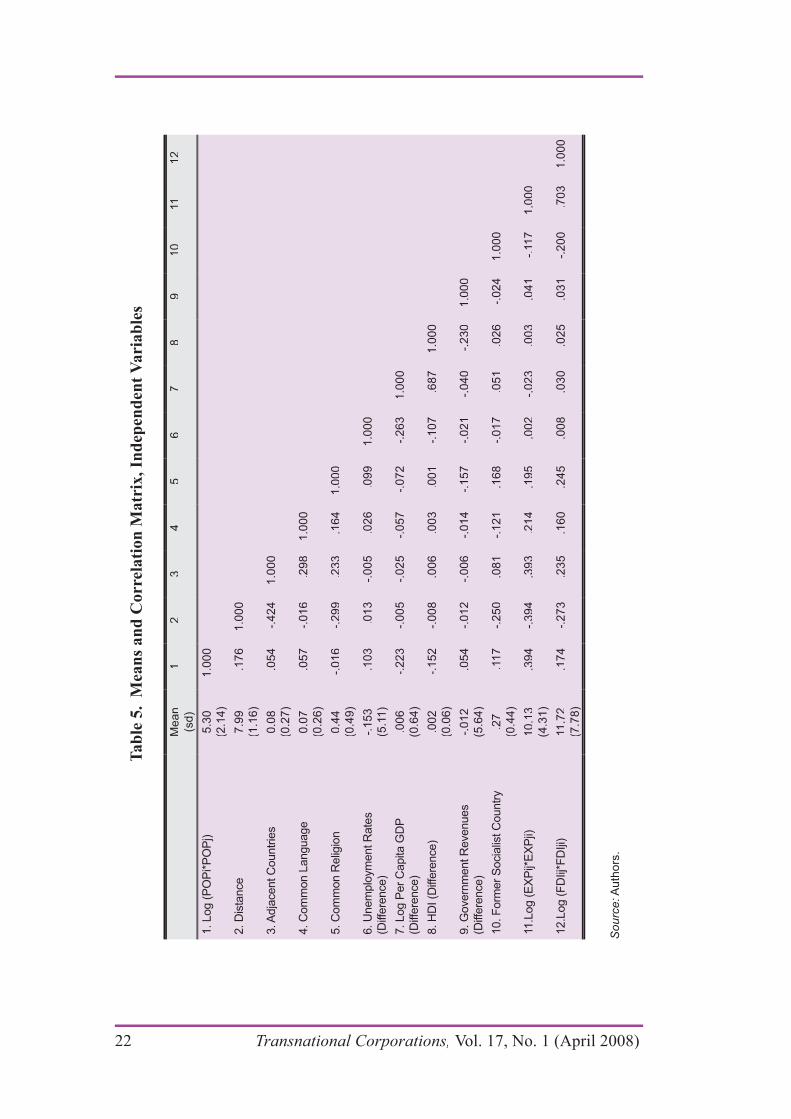
Table 5 reports the means and standard deviations (in parentheses)for the independent variables, as well as the correlation coefficientsamong the independent variables. The simple correlation coefficients arequite low with a few exceptions. One is the .703 correlation coefficient between the product term for bilateral exports between countries i and jand bilateral FDI between the two countries. The relatively strong positivecorrelation between bilateral trade and bilateral FDI is unsurprising. Asnoted earlier, the bulk of international trade among developed countriesis carried out by TNCs, and most previous studies indicate that FDI and trade are complements. Another strong correlation exists between thedifferences in per capita GDP between countries and the difference inscores of the HDI in the two countries. This is also not surprising giventhat the HDI includes GDP per capita. As a consequence, however, wedo not use HDI and GDP per capita in the same equation. We do include


Ta

ble

5.

Mea

ns

an

d C

orr

ela

tio

n M

atr

ix,

Ind

epen

den

t V

ari

ab

les

Mean

(sd)

12

34

56

78

910

11

12

1. Log (

PO

Pi*

PO

Pj)

1. Log (

PO

Pi*

PO

Pj)

5.3

05.3

0

(2.1

4)

(2.1

4)

1.0

00

1.0

00

2. D

ista

nce

2. D

ista

nce

7.9

97.9

9

(1.1

6)

(1.1

6)

.176

.176

1.0

00

1.0

00

3. A

dja

cent C

ountr

ies

3. A

dja

cent C

ountr

ies

0.0

80.0

8

(0.2

7)

(0.2

7)

.054

.054

-.424

-.424

1.0

00

1.0

00

4. C

om

mon L

anguage

4. C

om

mon L

anguage

0.0

70.0

7

(0.2

6)

(0.2

6)

.057

.057

-.016

-.016

.298

.298

1.0

00

1.0

00

5. C

om

mon R

elig

ion

5. C

om

mon R

elig

ion

0.4

40.4

4

(0.4

9)

(0.4

9)

-.016

-.016

-.299

-.299

.233

.233

.164

.164

1.0

00

1.0

00

6. U

nem

plo

ym

ent R

ate

s6. U

nem

plo

ym

ent R

ate

s

(Diff

ere

nce)

(Diff

ere

nce)

-.153

-.153

(5.1

1)

(5.1

1)

.103

.103

.013

.013

-.005

-.005

.026

.026

.099

.099

1.0

00

1.0

00

7. Log P

er

Capita

GD

P

7. Log P

er

Capita

GD

P

(Diff

ere

nce)

(Diff

ere

nce)

.006

.006

(0.6

4)

(0.6

4)

-.223

-.223

-.005

-.005

-.025

-.025

-.057

-.057

-.072

-.072

-.263

-.263

1.0

00

1.0

00

8. H

DI (D

iffere

nce)

8. H

DI (D

iffere

nce)

.002

.002

(0.0

6)

(0.0

6)

-.152

-.152

-.008

-.008

.006

.006

.003

.003

.001

.001

-.107

-.107

.687

.687

1.0

00

1.0

00

9. G

overn

ment R

evenues

9. G

overn

ment R

evenues

(Diff

ere

nce)

(Diff

ere

nce)

-.012

-.012

(5.6

4)

(5.6

4)

.054

.054

-.012

-.012

-.006

-.006

-.014

-.014

-.157

-.157

-.021

-.021

-.040

-.040

-.230

-.230

1.0

00

1.0

00

10. F

orm

er

Socia

list C

ountr

y10. F

orm

er

Socia

list C

ountr

y.2

7.2

7

(0.4

4)

(0.4

4)

.117

.117

-.250

-.250

.081

.081

-.121

-.121

.168

.168

-.017

-.017

.051

.051

.026

.026

-.024

-.024

1.0

00

1.0

00

11.L

og (

EX

Pij*

EX

Pji)

11.L

og (

EX

Pij*

EX

Pji)

10.1

310.1

3

(4.3

1)

(4.3

1)

.394

.394

-.394

-.394

.393

.393

.214

.214

.195

.195

.002

.002

-.023

-.023

.003

.003

.041

.041

-.117

-.117

1.0

00

1.0

00

12.L

og (

FD

Iij*F

DIji

)12.L

og (

FD

Iij*F

DIji

)11.7

211.7

2

(7.7

8)

(7.7

8)

.174

.174

-.273

-.273

.235

.235

.160

.160

.245

.245

.008

.008

.030

.030

.025

.025

.031

.031

-.200

-.200

.703

.703

1.0

00

1.0

00

Source: A

uth

ors

.


both FDI and trade in the same equation, but as reported below, theoutcome is problematic.

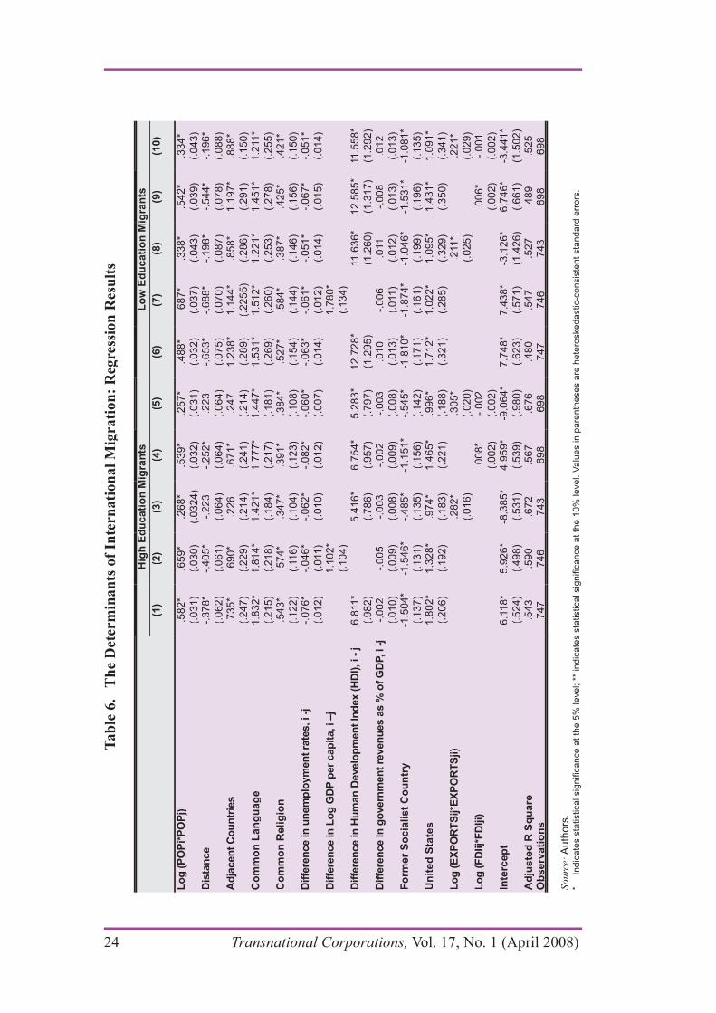
Table 6 reports regression results for two groups of migrants. Our primary focus is on highly educated migrants in a sample country i,born in another country j (FORH). These results are reported in columns(1) (5). We compare these results to a second sample, the total number of low education migrants in country i who originated in country j(FORL).25 These results are reported in columns (6) (10).26

Equations (1), (2), (5) and (6) report regression results of anaugmented gravity equation that excludes the bilateral export and bilateral FDI variables. The odd-numbered equations report estimatesusing HDI, while the even numbered ones replace that term with GDP per capita. In all four equations, all coefficients have the expected signs,and all are statistically significant, with the exception of the government revenues term. Although this particular result may reflect measurement error owing to the limitations on interpreting this variable as a measure of relative tax rates in the two countries, it is consistent with most previousresearch suggesting that differences in tax rates may not be significant influences on migration decisions.27

For the most part, all of the other independent variables in thefour equations are statistically significant at the .05 level. Of particular interest, higher unemployment rates in the host country relative to thehome country discourage migration, while higher relative standards of living/GDP per capita in the host country encourage migration. Variablesserving as proxies for lower costs of migration (physical distance,adjacency, common language and common religion) all perform asexpected, i.e. lower costs of migration significantly promote increased migration. However, we do not find that physical distance is a lesser deterrent to HEWs, as we had hypothesized. In contrast, the effects of language and religion are similar for both groups. Also, countries whichwere once officially “socialist” both sent and received lower number

25 We also estimated the same equations for the total sample of migrants, and for all migrants who are not HEWs. These results do not change our conclusions.

26

of observations is less than the potential number (29 x 28 = 812) country-pair observations.

27 Our measure of government revenues may also fail to accurately identify public

might be an indirect measure of public social expenditures.


Ta

ble

6.

T

he

Det

erm

ina

nts

of

Inte

rna

tio

na

l M

igra

tio

n:

Reg

ress

ion

Res

ult

s

Hig

h E

du

cati

on

Mig

ran

tsL

ow

Ed

ucati

on

Mig

ran

ts

(1)

(2)

(3)

(4)

(5)

(6)

(7)

(8)

(9)

(10)

Lo

g (

PO

Pi*

PO

Pj)

Lo

g (

PO

Pi*

PO

Pj)

.582*

.582*

(.031)

(.031)

.659*

.659*

(.030)

(.030)

.268*

.268*

(.0324)

(.0324)

.539*

.539*

(.032)

(.032)

.257*

.257*

(.031)

(.031)

.488*

.488*

(.032)

(.032)

.687*

.687*

(.037)

(.037)

.338*

.338*

(.043)

(.043)

.542*

.542*

(.039)

(.039)

.334*

.334*

(.043)

(.043)

Dis

tan

ce

Dis

tan

ce

-.378*

-.378*

(.062)

(.062)

-.405*

-.405*

(.061)

(.061)

-.223

-.223

(.064)

(.064)

-.252*

-.252*

(.064)

(.064)

.223

.223

(.064)

(.064)

-.653*

-.653*

(.075)

(.075)

-.688*

-.688*

(.070)

(.070)

-.198*

-.198*

(.087)

(.087)

-.544*

-.544*

(.078)

(.078)

-.196*

-.196*

(.088)

(.088)

Ad

jacen

t C

ou

ntr

ies

Ad

jacen

t C

ou

ntr

ies

.735*

.735*

(.247)

(.247)

.690*

.690*

(.229)

(.229)

.226

.226

(.214)

(.214)

.671*

.671*

(.241)

(.241)

.247

.247

(.214)

(.214)

1.2

38*

1.2

38*

(.289)

(.289)

1.1

44*

1.1

44*

(.2255)

(.2255)

.858*

.858*

(.286)

(.286)

1.1

97*

1.1

97*

(.291)

(.291)

.888*

.888*

(.150)

(.150)

Co

mm

on

Lan

gu

ag

eC

om

mo

n L

an

gu

ag

e1.8

32*

1.8

32*

(.215)

(.215)

1.8

14*

1.8

14*

(.218)

(.218)

1.4

21*

1.4

21*

(.184)

(.184)

1.7

77*

1.7

77*

(.217)

(.217)

1.4

47*

1.4

47*

(.181)

(.181)

1.5

31*

1.5

31*

(.269)

(.269)

1.5

12*

1.5

12*

(.260)

(.260)

1.2

21*

1.2

21*

(.253)

(.253)

1.4

51*

1.4

51*

(.278)

(.278)

1.2

11*

1.2

11*

(.255)

(.255)

Co

mm

on

Reli

gio

nC

om

mo

n R

eli

gio

n.5

43*

.543*

(.122)

(.122)

.574*

.574*

(.116)

(.116)

.347*

.347*

(.104)

(.104)

.391*

.391*

(.123)

(.123)

.384*

.384*

(.108)

(.108)

.527*

.527*

(.154)

(.154)

.584*

.584*

(.144)

(.144)

.387*

.387*

(.146)

(.146)

.425*

.425*

(.156)

(.156)

.421*

.421*

(.150)

(.150)

Dif

fere

nce in

un

em

plo

ym

en

t ra

tes, i -j

Dif

fere

nce in

un

em

plo

ym

en

t ra

tes, i -j

-.076*

-.076*

(.012)

(.012)

-.046*

-.046*

(.011)

(.011)

-.062*

-.062*

(.010)

(.010)

-.082*

-.082*

(.012)

(.012)

-.060*

-.060*

(.007)

(.007)

-.063*

-.063*

(.014)

(.014)

-.061*

-.061*

(.012)

(.012)

-.051*

-.051*

(.014)

(.014)

-.067*

-.067*

(.015)

(.015)

-.051*

-.051*

(.014)

(.014)

Dif

fere

nce in

Lo

g G

DP

per

cap

ita, i –j

Dif

fere

nce in

Lo

g G

DP

per

cap

ita, i –j

1.1

02*

1.1

02*

(.104)

(.104)

1.7

80*

1.7

80*

(.134)

(.134)

Dif

fere

nce in

Hu

man

Develo

pm

en

t In

dex (

HD

I), i -

jD

iffe

ren

ce in

Hu

man

Develo

pm

en

t In

dex (

HD

I), i -

j6.8

11*

6.8

11*

(.982)

(.982)

5.4

16*

5.4

16*

(.786)

(.786)

6.7

54*

6.7

54*

(.957)

(.957)

5.2

83*

5.2

83*

(.797)

(.797)

12.7

28

*12.7

28

*

(1.2

95)

(1.2

95)

11.6

36*

11.6

36*

(1.2

60)

(1.2

60)

12.5

85*

12.5

85*

(1.3

17)

(1.3

17)

11.5

58*

11.5

58*

(1.2

92)

(1.2

92)

Dif

fere

nce in

go

vern

men

t re

ven

ues a

s %

of

GD

P, i -j

D

iffe

ren

ce in

go

vern

men

t re

ven

ues a

s %

of

GD

P, i -j

-.

002

-.002

(.010)

(.010)

-.005

-.005

(.009)

(.009)

-.003

-.003

(.008)

(.008)

-.002

-.002

(.009)

(.009)

-.003

-.003

(.008)

(.008)

.010

.010

(.013)

(.013)

-.006

-.006

(.011)

(.011)

.011

.011

(.012)

(.012)

-.008

-.008

(.013)

(.013)

.012

.012

(.013)

(.013)

Fo

rmer

So

cia

list

Co

un

try

Fo

rmer

So

cia

list

Co

un

try

-1.5

04*

-1.5

04*

(.137)

(.137)

-1.5

46*

-1.5

46*

(.131)

(.131)

-.485*

-.485*

(.135)

(.135)

-1.1

51*

-1.1

51*

(.156)

(.156)

-.545*

-.545*

(.142)

(.142)

-1.8

10*

-1.8

10*

(.171)

(.171)

-1.8

74*

-1.8

74*

(.161)

(.161)

-1.0

46*

-1.0

46*

(.199)

(.199)

-1.5

31*

-1.5

31*

(.196)

(.196)

-1.0

81*

-1.0

81*

(.135)

(.135)

Un

ited

Sta

tes

Un

ited

Sta

tes

1.8

02*

1.8

02*

(.206)

(.206)

1.3

28*

1.3

28*

(.192)

(.192)

.974*

.974*

(.183)

(.183)

1.4

65*

1.4

65*

(.221)

(.221)

.996*

.996*

(.188)

(.188)

1.7

12*

1.7

12*

(.321)

(.321)

1.0

22*

1.0

22*

(.285)

(.285)

1.0

95*

1.0

95*

(.329)

(.329)

1.4

31*

1.4

31*

(.350)

(.350)

1.0

91*

1.0

91*

(.341)

(.341)

Lo

g (

EX

PO

RT

Sij*E

XP

OR

TS

ji)

Lo

g (

EX

PO

RT

Sij*E

XP

OR

TS

ji)

.282*

.282*

(.016)

(.016)

.305*

.305*

(.020)

(.020)

.211*

.211*

(.025)

(.025)

.221*

.221*

(.029)

(.029)

Lo

g (

FD

Iij*

FD

Iji)

Lo

g (

FD

Iij*

FD

Iji)

.008*

.008*

(.002)

(.002)

-.002

-.002

(.002)

(.002)

.006*

.006*

(.002)

(.002)

-.001

-.001

(.002)

(.002)

Inte

rcep

tIn

terc

ep

t6.1

18*

6.1

18*

(.524)

(.524)

5.9

26*

5.9

26*

(.498)

(.498)

-8.3

85*

-8.3

85*

(.531)

(.531)

4.9

59*

4.9

59*

(.539)

(.539)

-9.0

64*

-9.0

64*

(.980)

(.980)

7.7

48*

7.7

48*

(.623)

(.623)

7.4

38*

7.4

38*

(.571)

(.571)

-3.1

26*

-3.1

26*

(1.4

26)

(1.4

26)

6.7

46*

6.7

46*

(.661)

(.661)

-3.4

41*

-3.4

41*

(1.5

02)

(1.5

02)

Ad

juste

d R

Sq

uare

Ad

juste

d R

Sq

uare

.543

.543

.590

.590

.672

.672

.567

.567

.676

.676

.480

.480

.547

.547

.527

.527

.489

.489

.525

.525

Ob

serv

ati

on

sO

bserv

ati

on

s747

747

746

746

743

743

698

698

698

698

747

747

746

746

743

743

698

698

698

698

So

urc

e: A

uth

ors

.*

Indic

ate

s s

tatistical sig

nific

ance a

t th

e 5

% level; *

* in

dic

ate

s s

tatistical sig

nific

ance a

t th

e 1

0%

level. V

alu

es in p

are

nth

eses a

re h

ete

roskedastic-c

onsis

tent sta

ndard

err

ors

.


of migrants, other things equal, while the United States received moreimmigrants of all kinds.

In equations (3) (5), and (8) (10), the product terms for bilateraltrade and FDI are added, first one at a time and then together. For thesepurposes, we use the more general HDI measure, but the results aresimilar when GDP per capita is used in these same equations. Whenentered alone, both the trade and FDI terms are positive, and statisticallysignificant in all equations. For the most part, all other variables areunaffected by the addition of these terms. In addition, while both termsadd to the explanatory power of the model, the addition of the trade termcreates a substantial increase in the R2 (compare columns 1 and 3; 5 and 8). Thus, comparable estimation results for the two sets of coefficientsreinforce our interpretation of the linkages between FDI, trade and migration. Specifically, the human capital of HEWs is complementaryto other assets possessed by TNCs that facilitate profitable trade and FDI carried out primarily by those same TNCs. Although trade and FDIalso affect low education migration, the effects are less pronounced, aresult discussed further below.

Equations (5) and (10) include both bilateral trade flows and bilateral FDI flows in the estimating equation. Given the strong correlationbetween the two variables, there is a concern about multicollinearity, and it is perhaps not surprising that only one is statistically significant: the trade variable. On the surface, the result suggests that trade flows are amore important determinant of HEW migration than FDI flows; however,it is impossible, as a practical matter, to separately identify the impact of trade versus FDI on HEW migration when the bulk of internationaltrade is carried out by TNCs. In addition, the potential measurement issues regarding bilateral FDI noted above contribute to the uncertaintyregarding the precise strength of its influence on migration.

A question that might be asked is whether trade carried out by TNCs has a stronger effect on HEW migration than inter-firm trade. To gain some insight into this issue, we replaced the bilateral FDI variablein equations (5) and (10) with an interaction variable, the bilateraltrade variable multiplied by the bilateral FDI variable (not reported).In this specification, if the coefficient for the interaction variable ispositive and statistically significant, it would indicate that intra-firmtrade undertaken by TNCs has a greater impact on HEW migration thantrade in general. However, this variable proved not to be statisticallysignificant in either equation. Taken at face value, this latter result suggests that the complementary relationship between migration and


trade is not necessarily enhanced when trade takes the form of intra-firmexports and imports within TNCs.

In general, the results for the low education migration equationsare qualitatively similar to those for the highly educated migrants evenwhen the multiplicative trade and FDI terms are added. However, themagnitude and statistical significance of some key coefficients does varyacross the sets of equations. Thus, there are some important factors that distinguish HEW migrants from others. The most of important of theseare the effects of physical distance, national income (HDI), trade and FDI. HEWs are less constrained by the costs associated with physicaldistance. They are also less attracted by differences in living standards.The larger coefficient for the HDI term for low education migrants (alsofound for GDP per capita) implies that less well educated migrantsare more responsive to pecuniary income differences across countries,whereas highly educated workers are more likely to move to countrieswith more comparable standards of living. At the same time, HEWs aremore attracted by bilateral trade and FDI (though the latter difference isnot statistically significant), as we hypothesized. However, one of thepossible expected differences discussed in the previous section is not evident. The coefficient for common language is somewhat greater for the highly educated migrant cohort. Although this result is not what wasexpected, it perhaps reflects the fact that highly educated migrants aremore likely to pursue jobs that require a high degree of literacy, therebyrequiring fluency or near-fluency in the language of the host country.28

As discussed in the previous section, an important specificationissue in gravity models is whether variables expressed as differencesor log products should be entered separately. We therefore estimated models in which all relevant variables (unemployment rates, HDI,GDP per capita, government revenues, bilateral trade and bilateral FDI)were included in unrestricted form. For example, in the case of HDI,the unrestricted specification includes both HDIi and HDIj, whereasthe restricted specification includes (HDIi - HDIj). In the case of FDI,the restricted specification is log (FDIij*FDIji) whereas the unrestricted specification includes log FDIij and log FDIji individually. However,specifications involving both FDI terms were problematic because theterms are highly collinear and, when entered separately, the coefficient

28

migrants. They also report that high-skill workers are more affected by differences interms of living standards compared to unskilled workers, although emigration rates for both are negatively related to physical distance and to the unemployment rate at the


on one or both is not statistically significant. The same was true for the export terms. 29 As a consequence, we could include only one FDI(and export) term in each specification. Given our speculation that flowsfrom j to i are likely to be more important influences on HEW migration,we adopted a final specification that includes only exports and FDI fromj to i (home to host).30 These results are presented in table 7.

Since GDP per capita and HDI could not be included in thesame equation, we report separate specifications using each variable.Similarly, since the FDI and trade terms could not be entered together,we report results separately for each. Since the results were similar for all cases, we report the trade equations using GDP per capita, and theFDI equations using HDI. We report each equation for the most highlyeducated migrants (FORH), and the least highly educated migrants

For comparable variables, the results reported in table 7 are not very much different from those discussed above. However, the resultsin table 7 also reveal greater differences among migrants with different levels of education. In particular, the trade and FDI terms are still moreimportant for HEWs, but the differences are more pronounced and arestatistically significant. Moreover, it is clear that “pull” factors (thoseassociated with the host country, i) are relatively more influential for highly educated migrants. In contrast, “push” factors (those associated with the home country, j) are relatively more important for migrants inthe lowest education category. For the most part, unemployment rates,GDP per capita and HDI in country i are more important relative to the comparable effects in country j for those with the highest levels of jeducation.31

These results suggest that highly educated migrants are likelyto do well in their home country, and therefore require more positiveincentives to re-locate. In addition, they are likely to have moreinformation about host country markets. Those with lower levels of

29 As a consequence, the outcome of F-tests comparing restricted and unrestricted

reported in table 6) is tested against an unrestricted model which includes both FDIterms, the restricted model is accepted. When only one FDI term is included in theunrestricted model, the latter is accepted.

30 We also estimated models with only the reverse (i to jbut do not present them. They are discussed in the text.

31

(2006).


education leave when local conditions deteriorate, and may have lessinformation about potential destinations.

The estimated coefficients for the United States dummy variableare suggestive, inasmuch as they indicate that the United States attractsmore of all types of migrants, holding other factors constant. The resultsare consistent with our speculation that migrants at all educational levelswho view themselves as potentially above-average performers in thereceiving country see greater economic opportunities in the United Statesthan in other countries beyond the differences suggested by disparitiesin average wage or income levels.

The results in table 7 continue to indicate that FDI and trade areimportant determinants of migration flows, and that both variables aremore strongly related to the migration of HEWs than other migrants.However, these results focus on the flows from j toj i. When we estimate the equations including only trade and FDI flows from i to j, the results are weaker, as we had speculated. Although both variables are positiveand statistically significant in all equations, the evidence that they have agreater effect on HEWs is weaker. In addition, because of the collinearityassociated with these variables, we are unable to say whether the tradeand FDI effects are best captured by the total size of the FDI and tradenetworks (the interactive product term) or by individual bilateral tradeand FDI effects. This issue should be pursued in subsequent research.

As discussed above, there is reason to believe that the potentialendogeneity of the FDI and trade variables may create biased estimates,and that our results might not be robust to specifications that account for the potential endogeneity of these variables. Thus, unobserved variables may simultaneously affect immigration, trade and FDI, and/or two-way causality may exist. For example, unobserved heterogeneityacross countries may result in simultaneous movement of capital, goodsand people, or strong trade and FDI links may result from immigration.As a consequence, we adopted an instrumental variables estimationprocedure, using a method initially proposed by Evans and Kessides(1993), but more recently employed by Edwards and Waverman (2006)and Cubbin and Stern (2006).

We constructed a rank based instrument for all trade and FDIvariables, including the interaction terms reported in tables 6 and 7.For example, following Edwards and Waverman (2006), we sorted the log (FDIij*FDIji) variable into three ranks (1, 2, 3) and so created


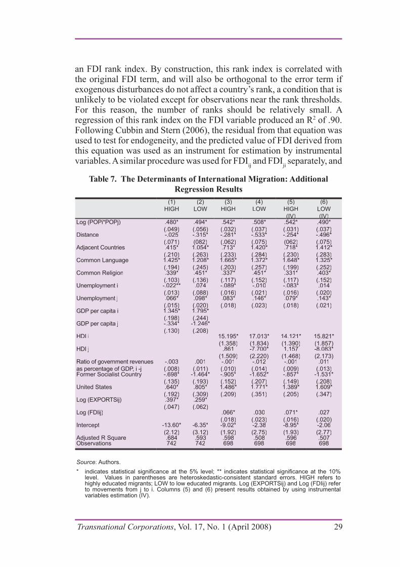
an FDI rank index. By construction, this rank index is correlated withthe original FDI term, and will also be orthogonal to the error term if exogenous disturbances do not affect a country’s rank, a condition that isunlikely to be violated except for observations near the rank thresholds.For this reason, the number of ranks should be relatively small. A regression of this rank index on the FDI variable produced an R2 of .90.Following Cubbin and Stern (2006), the residual from that equation wasused to test for endogeneity, and the predicted value of FDI derived fromthis equation was used as an instrument for estimation by instrumentalvariables. A similar procedure was used for FDI

ij and FDI

jiI separately, and

Table 7. The Determinants of International Migration: Additional

Regression Results

(1)

HIGH

(2)

LOW

(3)

HIGH

(4)

LOW

(5)

HIGH

(IV)( )( )(IV)( )( )

(6)

LOW

(IV)( )( )(IV)( )( )Log (POPi*POPj)Log (POPi*POPj) .480*.480*

(.049)(.049)

.494*.494*

(.056)(.056)

.542*.542*

(.032)(.032)

.508*.508*

(.037)(.037)

.542*.542*

(.031)(.031)

.490*.490*

(.037)(.037)DistanceDistance -.025-.025

(.071)(.071)

-.315*-.315*( )( )))

(082)(082)

-.281*-.281*( )( )))

(.062)(.062)

-.533*-.533*( )( )))

(.075)(.075)

-.254*-.254*( )( )))

(062)(062)

-.496*-.496*( )( )))

(.075)(.075)Adjacent CountriesAdjacent Countries .415*.415*

( )( )

(.210)(.210)

1.054*1.054*( )( )

(.263)(.263)

.713*.713*( )( )

(.233)(.233)

1.420*1.420*( )( )))

(.284)(.284)

.718*.718*( )( )))

(.230)(.230)

1.412*1.412*( )( )))

(.283)(.283)Common LanguageCommon Language 1.425*1.425*

( )( )( )( )

(.194)(.194)

1.208*1.208*( )( )( )( )

(.245)(.245)

1.665*1.665*( )( )( )( )

(.203)(.203)

1.372*1.372*( )( )( )( )

(.257)(.257)

1.648*1.648*( )( )( )( )

(.199)(.199)

1.325*1.325*( )( )( )( )

(.252)(.252)Common ReligionCommon Religion .339*.339*

( )( )

(.103)(.103)

.451*.451*( )( )

(.136)(.136)

.337*.337*( )( )

(.117)(.117)

.451*.451*( )( )

(.152)(.152)

.331*.331*( )( )

(.117)(.117)

.403*.403*( )( )

(.152)(.152)Unemployment iUnemployment i -.022**-.022**

( )( )

(.013)(.013)

.074.074

(.088)(.088)

-.089*-.089*( )( )))

(.016)(.016)

-.010-.010

(.021)(.021)

-.083*-.083*( )( )))

(.016)(.016)

.014.014

(.020)(.020)Unemployment jUnemployment j .066*.066*

( )( )

(.015)(.015)

.098*.098*( )( )

(.020)(.020)

.083*.083*( )( )

(.018)(.018)

.146*.146*( )( )

(.023)(.023)

.079*.079*( )( )

(.018)(.018)

.143*.143*( )( )

(.021)(.021)GDP per capita iGDP per capita i 1.345*1.345*

( )( )( )( )

(.198)(.198)

1.795*1.795*( )( )( )( )

(.244)(.244)GDP per capita jGDP per capita j -.334*-.334*

( )( )))

(.130)(.130)

-1.246*-1.246*( )( )

(.208)(.208)HDI iHDI i 15.195*15.195*

(1.358)(1.358)

17.013*17.013*

(1.834)(1.834)

14.121*14.121*

(1.390)(1.390)

15.821*15.821*

(1.857)(1.857)HDI jHDI j .861.861

(1.509)(1.509)

-7.700*-7.700*( )( )))

(2.220)(2.220)

1.1571.157

(1.468)(1.468)

-8.083*-8.083*( )( )))

(2.173)(2.173)Ratio of government revenuesRatio of government revenues

as percentage of GDP, i -j as percentage of GDP, i -j

-.003-.003

(.008)(.008)

.001.001

(.011)(.011)

-.001-.001

(.010)(.010)

-.012-.012

(.014)(.014)

-.001-.001

(.009)(.009)

.011.011

(.013)(.013)Former Socialist CountryFormer Socialist Country

g jg jgg-.698*-.698*( )( )))

(.135)(.135)

-1.464*-1.464*( )( )

(.193)(.193)

-.905*-.905*( )( )))

(.152)(.152)

-1.652*-1.652*( )( )

(.207)(.207)

-.857*-.857*( )( )))

(.149)(.149)

-1.531*-1.531*( )( )

(.208)(.208)United StatesUnited States .640*.640*

( )( )

(.192)(.192)

.805*.805*( )( )

(.309)(.309)

1.486*1.486*( )( )))

(.209)(.209)

1.771*1.771*( )( )))

(.351)(.351)

1.389*1.389*( )( )))

(.205)(.205)

1.609*1.609*( )( )))

(.347)(.347)Log (EXPORTSij)Log (EXPORTSij) .397*.397*

( )( )

(.047)(.047)

.259*.259*( )( )

(.062)(.062)Log (FDIij)Log (FDIij) .066*.066*

(.018)(.018)

.030.030

(.023)(.023)

.071*.071*

(.016)(.016)

.027.027

(.020)(.020)InterceptIntercept -13.60*-13.60*

(2.12)(2.12)

-6.35*-6.35*

(3.12)(3.12)

-9.02*-9.02*( )( )))

(1.92)(1.92)

-2.38-2.38

(2.75)(2.75)

-8.95*-8.95*( )( )))

(1.93)(1.93)

-2.06-2.06

(2.77)(2.77)Adjusted R SquareAdjusted R Square .684.684 .593.593 .598.598 .508.508 .596.596 .507.507ObservationsObservations

jjjj742742 742742 698698 698698 698698 698698

Source: Authors.

* indicates statistical significance at the 5% level; ** indicates statistical significance at the 10%level. Values in parentheses are heteroskedastic-consistent standard errors. HIGH refers tohighly educated migrants; LOW to low educated migrants. Log (EXPORTSij) and Log (FDIij) refer to movements from j to i. Columns (5) and (6) present results obtained by using instrumentalvariables estimation (IV).


for the trade terms. We adopted this technique because of the difficultyin finding suitable and different instruments (different variables that areboth correlated with the suspected endogenous variable and uncorrelated with the error term) for both the trade and FDI terms.32

The results suggest that although the trade and FDI terms areendogenous, the instrumental variables estimates are not different in anymaterial way from the OLS estimates reported in tables 6 and 7. As anexample, we provide one set of estimates in columns (5) and (6) of table7. Other results are similar in that none of the estimated coefficientsare impacted in any significant way through estimation by instrumentalvariables.33

6. Summary and conclusions

In this study, we specify and estimate an augmented gravity modelof the determinants of bilateral migration flows across OECD countries.Our specific focus is on HEWs, and the impact on migration of bilateraltrade and FDI. We argue that TNCs are efficient, direct channels for themovement of HEWs across international borders. This study adds to theliterature in two main ways. First, it employs relatively recent data that distinguish migrants by level of education. Second, it includes measuresof both bilateral trade and FDI as determinants of bilateral migrationflows.

The primary migration data employed in this study are based on the stock of foreign born individuals from country j in countryj i,organized by level of education. There is a relatively high level of correlation among the various education categories: countries with highnumbers of foreign born from a specific home country tend to have highnumbers for all education groups. We speculate that this may be linked to the importance of immigration networks within a host country that provide cultural amenities and other forms of support.

Our results indicate that bilateral migration flows for migrants at all levels of education are well explained by a basic gravity model. In particular, migration is greatest between countries with large populations,

32 The chosen instruments must still be approached with some caution. In particular,

over the years.33 These results are available on request.


and is reduced when geographic, linguistic and religious distances arehigh. Migration is also influenced by relative labour market conditions.Specifically, migrants tend to leave countries where economic conditionsare relatively poor (high unemployment; low GDP per capita) and move to areas where conditions are better. Our results also confirm theimportance of FDI and trade as determinants of migration flows. We find that both are complements to migration. In general, we find noevidence that higher levels of bilateral trade or FDI replace movementsof labour. This stands in contrast to Gonzales and Maloney (2005) whoinclude both trade and FDI variables in their examination of migrationwithin Mexico and find that they are substitutes. Clearly, more researchon this issue is required.

Finally, our results indicate that there are important differencesin the determinants of migration outcomes, by level of education. Inparticular, highly educated workers are less constrained by physicaldistance and are more likely to move to countries with similar standardsof living. Importantly, highly educated migrants are more influenced by the “pull” of economic conditions in host countries. In contrast,workers with less education are more heavily influenced by the “push”of economic factors in their home countries. We also find evidence that highly educated migration is more responsive to bilateral trade and FDIflows. All results are robust to correction for the potential endogeneityof trade and FDI variables.

An important policy implication of our results is that macroeconomic performance is an important determinant of migration.In particular, a robust labour market and a rising real income levelare strong attractions for migrants, especially HEWs. As is true in somany areas of economic policy, conditions encouraging real economicgrowth stimulate investment decisions that contribute further to futurereal economic growth. In this regard, while an increasing number of developed countries have been focusing on specialized programmesto encourage immigration of HEWs, it may well be that conventionalpublic policies focused on promoting long-run real economic growthare more powerful factors encouraging the immigration of HEWs. At the same time, these same policies should also encourage the retentionof native-born HEWs

Perhaps the most important policy inference emerging from thisstudy is that policies to promote deeper trade and investment integrationhave important implications for attracting and retaining HEWs, as well asother migrants. Most trade agreements, particularly bilateral agreements,


have traditionally focused on reducing barriers to the movement of goodsand capital. Our results suggest that this focus is incomplete because it ignores a major complement to trade and investment, namely migration.By ignoring or minimizing the importance of provisions for liberalized migration most trade agreements are therefore arguably failing to exploit the full benefits arising from the complementarity among increased international flows of goods, capital and highly educated workers.

References

Aroca, P. and W.F. Maloney (2004). “Migration, trade and FDI in Mexico”, Washington,D.C.: World Bank, mimeo.

Borjas, G.J. (1987). “Self-selection and the earnings of immigrants”, American EconomicReview, 77, pp. 531 553.

Links between migration and German FDI”, Working Paper, No. 1190, Kiel.

Checchi, Daniele, Gianfranco De Simone and Ricardo Faini (2007). “Skilled migration,FDI and human capital investment”, Discussion Paper, No. 2795, Bonn: IZA.

Chen, Natalie (2004). “Intra-national versus international trade in the European Union:Journal of International Economics, 63(1), pp.

93–118.

Combes, Pierre-Philippe, Miren Lafourcade and Thierry Mayer (2005). “The trade-creating effects of business and social networks: evidence from France”, Journal of International Economics, 66(1), pp. 1–29.

Cubbin, John and Jon Stern (2006). “The impact of regulatory governance and privatization on electricity industry generation capacity in developing economies” ,World Bank Economic Review, 20(1), pp. 115–141.

Docquier, F. (2006). “Brain drain and inequality across nations”. Paper prepared for the EUDN-AFD conference on “Migration and Development”, Paris, 8 November 2006, mimeo.

Working Paper, No. 31, Paris: Agence Francaise de Developpment.

Docquier, F. and A. Marfouk (2004). “Measuring the international mobility of skilled workers (1990–2000)”, Policy Research Working Paper, No. 3381, Washington,D.C.: World Bank.

Docquier, F. and A. Marfouk (2006). “International migration by education attainment,1990–2000”, in C. Ozden and M. Schiff, eds., International Migration, Remittancesand the Brain Drain, Washington, D.C. and NewYork: World Bank and PalgraveMacmillan, pp. 151–199.

Docquier, F. and Elisabetta Lodigiani (2007). “Skilled Migration and Business Networks”Available at SSRN: http://ssrn.com/abstract=1002649


Dostie, Benoit and Pierre Thomas Leger (2004). “A critical review of the microeconomicmigration literature”, Working Paper, 2004 D-05, Ottawa: Government of Canada,Skills Research Initiative.

Dumont, J.C. and G. Lemaitre (2004). “The OECD database on expatriates and theforeign born”, The Statistics Newsletter, OECD, October.

Dumont, J.C. and G. Lemaitre (2005). “Counting immigrants and expatriates in OECDCountries: a new perspective”, OECD Social Employment and Migration Working Papers, No. 25, Paris: OECD Directorate for Employment, Labour and SocialAffairs.

Edwards, G.E. and L. Waverman (2006). “The effects of public ownership and regulatoryindependence on regulatory outcomes”, Journal of Regulatory Economics, 29(1), pp. 23–67.

Eichengreen, Barry and Douglas Irwin (1998). “The role of history in bilateral tradeThe Regionalization of the World Economy, Chicago:

University of Chicago Press, pp. 33–57.

Evans, W. and I. Kessides (1993). “Localized market power in the US airline industry”,Review of Economics and Statistics, 75(1), pp. 66–73.

Forster, Michael and Marco Mira d’Ecole (2005). “Income distribution and poverty inOECD countries in the second half of the 1990s”, Social, Employment and MigrationWorking Papers, No. 22, Paris: OECD.

Frankel, Jeffrey and Andrew Rose (2002). “An estimate of the effects of commoncurrencies on trade and income”, Quarterly Journal of Economics, May, pp. 437–466

Gonzalez, Patricio Aroca and William F. Maloney (2005). “Migration, trade and foreigndirect investment in Mexico”, Research Working Paper, No. 3601, Washington,D.C.: World Bank.

Globerman, Steven (1994). “Immigration and trade” in Don J. DeVoretz, ed. DiminishingReturns, Toronto: C.D. Howe Institution, pp. 243–267.

the role of governance infrastructure”, World Development, 30(11), pp. 1898–1919.

Gould, D. (1994). “Immigrant links to home country: empirical implications for U.S.Review of Economics and Statistics, 76, pp. 302–316.

Head, Keith and John Ries (1998). “Immigration and trade creation: econometricevidence from Canada”, Canadian Journal of Economics, XXXI(1), pp. 47–62.

Head, Keith and John Ries (2001). “Increasing returns versus national product differentiation as an explanation for the pattern of U.S.-Canada trade”, AmericanEconomic Review, 91(4), pp. 858–876.

Head, Keith and John Ries (2004). “Making Canada the destination of choice for internationally mobile resources”, Discussion Paper, No. 14, Industry Canada,January


Hejazi, Walid and Peter Pauly (2005). “How do regional trade agreements affect intra-

Governance, Multinationals and Growth, London: Edward Elgar, pp. 176–209.

Hejazi, Walid and A.E. Safarian (2001). “The complementarity between U.S. FDI stock and trade”, Atlantic Economic Journal, 29(4), pp. 420–437.

Karemera, David, Victor Iwuagwu Oguledo and Bobby Davis (2000). “A gravity modelanalysis of international migration to North America”, Applied Economics, 32, pp.1745–1755.

Economics Letters, 94(2), pp. 155–162.

Lopes, Sandra (2004). “Canadian business perspectives on the international mobility of skilled labour”, Skills Research Initiative Working Paper, No. 2004, D-03, Ottawa:Government of Canada.

Lowry, Ira (1966). Migration and Metropolitan Growth: Two Analytical Models, SanFrancisco: Chandler

Mahroun, Sami (1999). “Highly skilled globetrotters: the international migration of

Mayda, Anna Maria (2005). “International migration: a panel data analysis of economicand non-economic determinants”, IZA Discussion Paper, No. 1590, May

Mayer, Thierry and Soledad Zignano (2006). “Notes on CEPII’s distance measures”,May 2006 (available at http://www.cepii.fr/distance/noticedist_en.pdf).

they march to the same tune”, Canadian Journal of Economics, 31(4), pp. 778–800.

OECD (2002). Trends in International Migration, Paris: OECD Editions.

Pedersen, Peder, Mariola Pytlikova and Nina Smith (2004). “Selection or network

April.

Peri, Giovanni (2005). “International Migrations: some comparisons and lessons for theEuropean Union”, Davis: University of California, mimeo.

Rauch, J. (2001). “Business and social networks in international trade”, Journal of Economic Literature, 39, pp. 1177–1203.

Rauch, J. and V. Trinidade (2002). “Ethnic Chinese networks in international trade”,Review of Economics and Statistics, 84(1), pp. 116–130.

Salt, J. and J. Clarke (1998). “Flows and stocks of foreign labour in the UK”, LabourMarket Trends, July.

Sen, A. and T.E. Smith (1995). Gravity Models of Spatial Interaction Behavior, NewYork: Springer.

Slangen, Arjen, Sjoerd Beugelsdijk and Jean-Francois Hennart (2004). “National cultural


Tremblay, Karine (2004). “Links between academic mobility and integration”. Paper presented at “Symposium on International Labour and Academic Mobility: EmergingTrends and Implications for Public Policy”, Toronto, 20 October.

Wagner, Don (2000). “Do tax differences contribute toward the brain drain from Canada

Vancouver.

Zipf, George Kingsley (1946). “The P1P

2/D hypothesis: on the intercity movement of

persons”, American Sociological Review, II(December), pp. 677–686.


The international mobility of highly educated …unctad.org/en/docs/iteiit20081a2_en.pdfThe...

Documents

Transcript of The international mobility of highly educated …unctad.org/en/docs/iteiit20081a2_en.pdfThe...