energies

Article

The Integration of 3D Modeling and Simulation toDetermine the Energy Potential of Low-TemperatureGeothermal Systems in the Pisa (Italy)Sedimentary Plain

Alessandro Sbrana 1,*, Paola Marianelli 1,* ID , Giuseppe Pasquini 1, Paolo Costantini 1,Francesco Palmieri 2 ID , Valentina Ciani 3 and Michele Sbrana 3

1 Dipartimento di Scienze della Terra, University of Pisa, Via S. Maria 53, 56126 Pisa, Italy;giuseppe.pasquini@dst.unipi.it (G.P.); paolo.costantini@dst.unipi.it (P.C.)

2 Istituto Nazionale di Oceanografia e di Geofisica Sperimentale—OGS, Borgo Grotta Gigante 42/C,34010 Sgonico (TS), Italy; fpalmieri@inogs.it

3 Terra Energy, Via Lenin 132-56017 San Giuliano Terme (PI), Italy; ciani@terra-energy.it (V.C.);m.sbrana@terra-energy.it (M.S.)

* Correspondence: alessandro.sbrana@unipi.it (A.S.); paola.marianelli@unipi.it (P.M.)

Received: 15 May 2018; Accepted: 14 June 2018; Published: 18 June 2018�����������������

Abstract: Shallow, low-temperature geothermal resources can significantly reduce the environmentalimpact of heating and cooling. Based on a replicable standard workflow for three-dimensional (3D)geothermal modeling, an approach to the assessment of geothermal energy potential is proposed andapplied to the young sedimentary basin of Pisa (north Tuscany, Italy), starting from the developmentof a geothermal geodatabase, with collated geological, stratigraphic, hydrogeological, geophysicaland thermal data. The contents of the spatial database are integrated and processed using softwarefor geological and geothermal modeling. The models are calibrated using borehole data. Modeloutputs are visualized as three-dimensional reconstructions of the subsoil units, their volumes anddepths, the hydrogeological framework, and the distribution of subsoil temperatures and geothermalproperties. The resulting deep knowledge of subsoil geology would facilitate the deployment ofgeothermal heat pump technology, site selection for well doublets (for open-loop systems), or verticalheat exchangers (for closed-loop systems). The reconstructed geological–hydrogeological models andthe geothermal numerical simulations performed help to define the limits of sustainable utilization ofan area’s geothermal potential.

Keywords: 3D modeling; 3D numerical simulation; geographic information systems (GIS)geodatabase; geothermal potential assessment; shallow geothermal

1. Introduction

Sustainability, including in urban areas, has become a key concern when planning for the future [1].Increasing energy demand, the changing climate, and energy resources limitations have promptedseveral countries to introduce strategies to enhance energy-efficiency and production sustainability.The construction and ongoing use of the built environment are substantial contributors to growingenergy demand, using from 20 to 40% of the energy consumed in developed countries and accountingfor more than 30% of total greenhouse emissions [1,2]. In Europe, the Directive on Energy Performanceof Buildings [3] states that all new constructions should be “zero-energy buildings” by the end of2020. This implies buildings that consume minimum levels of renewably sourced energy. By replacingfossil fuel sources and substantially reducing the CO2 emissions, renewable energy sources help

Energies 2018, 11, 1591; doi:10.3390/en11061591 www.mdpi.com/journal/energies

Energies 2018, 11, 1591 2 of 20

mitigate global warming. Low temperature geothermal resources, as used for heating and cooling(via geothermal heat pumps [GHPs]), are one of the renewable sources that can contribute to energyefficiency and greenhouse gas reduction, while having only marginal negative environmental effects.Best practice in geothermal exploration, including quantitative assessment of geothermal plays [4],is a key step towards sustainable power generation. Multidisciplinary spatial data (including regionalgeological, stratigraphic, structural, geophysical and volumetric data) with temperature measurementsand hydrogeological and geothermal parameters derived from wells and exploratory boreholes areessential to reliable assessment. Accurate three-dimensional modeling considering the heterogeneityof the environment requires integration of diverse data sources [5–7]. The contributing technologiesinclude smart geographic information systems, their databases, 3D geological modeling, and 3Dnumerical simulation tools, which are already widely used and tested in research and the geothermalindustry. GIS applications in geothermal exploration are common, especially in the planning phase forsite selection [8] and for calculating and mapping the geothermal potential [9,10]. Papers on modelingin the geothermal domain commonly focus on data integration and elaboration, and visualization in3D modeling platforms [11–13]. These papers highlight the importance of 3D modeling, combiningmultiple datasets and procedures, and thus demonstrate the value of these tools in the management ofgeothermal resources. The integration of 3D modeling tools with 3D geothermal reservoir simulationtools is less common, although some authors [14,15] have studied both low- and high-enthalpygeothermal systems.

This paper proposes a methodology for robust 3D geological modeling and tests its applicationin a low-temperature environment. The model outputs are necessary for estimation of the potentialfor effective deployment of ground source heat pumps and to support the design of efficientlow-temperature geothermal plants. Geothermal simulations, when compared with direct, spatiallydistributed measurements in aquifers, provide for model calibration and hence accurate geothermalproject analysis.

Our case study area is the Pisa alluvial plain located north of the Tuscany (Italy) geothermal district.This area is characterized by a geothermal gradient of 50–60 ◦C·km−1 [16,17] and by fault-driventhermal springs. This is a typical low-temperature geothermal play, which is suitable for direct use ofGHPs for heating and cooling.

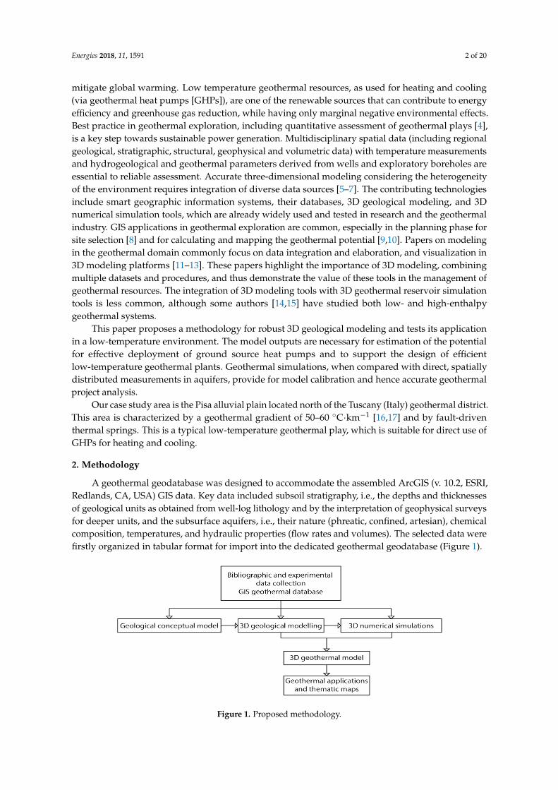
2. Methodology

A geothermal geodatabase was designed to accommodate the assembled ArcGIS (v. 10.2, ESRI,Redlands, CA, USA) GIS data. Key data included subsoil stratigraphy, i.e., the depths and thicknessesof geological units as obtained from well-log lithology and by the interpretation of geophysical surveysfor deeper units, and the subsurface aquifers, i.e., their nature (phreatic, confined, artesian), chemicalcomposition, temperatures, and hydraulic properties (flow rates and volumes). The selected data werefirstly organized in tabular format for import into the dedicated geothermal geodatabase (Figure 1).

Energies 2018, 11, x FOR PEER REVIEW 3 of 20

interpolation algorithm consists of three steps: (1) Refine—increase grid resolution; (2) Snap—regrid

the data; and (3) Smooth—minimize curvature of the grid [18].

Starting with the upper surfaces, a 3D grid was used as the basis of a 3D geological model of the

investigated area. The initial conceptual model was revised using improved 3D elaboration and

visualization: For example, lithostratigraphic and well log data can suggest adjustments to the

geothermal geodatabase, while the 3D reconstruction of aquifers allows the conceptual model to be

further modified and improved. The refined geological conceptual model and the resultant 3D Petrel

subsurface model became the framework for subsequent geothermal simulations. The top surfaces of

the subsurface units, from the 3D modeling, were imported into TOUGH2 [19] through the PetraSim

(version 5; Rockware Inc, Golden, CO, USA) graphical interface. TOUGH2 is a non-isothermal

multiphase fluid flow simulator for modeling heat and mass transfer in geothermal systems. In this

study, the EOS1 module was used. The computational approach used in TOUGH2 is based on the

integral finite difference (IFD) method [20] using fully implicit time discretization. The residual form

of the system of equations, considering the underground lithological setting, the heat flow dynamics,

and the heat exchange and fluid mass transport laws, is solved using the Newton–Raphson iteration

method [21]. Geothermal parameters, including density, porosity, permeability, heat conductivity,

and specific heat (both literature-derived values and in situ measurements), were assigned as input

data to subsoil units. The boundary conditions were set as for a closed system. A grid size was chosen

for the calculation based on the required spatial resolution and the acceptable computational load.

The simulation then modeled the steady state of the subsoil volume.

Temperature data, as measured in water, geothermal, and deep oil and gas exploratory wells,

were used to check the thermal settings of the model. Several iterations were performed to obtain the

best fit between measured and simulated temperature data. The distribution of output temperatures,

obtained through the TOUGH2 simulation, was transferred back to the Petrel software, allowing

visualization of the 3D distribution of subsoil temperatures in the aquifer or geological units (along

the X-, Y-, or Z-axis, in 2D sections or as well logs). Further, the simulated temperatures may be

integrated with temperature values measured in existing wells, giving a robust picture of the 3D

temperature distribution in the subsoil. These temperatures were interpolated to a continuous raster

surface, using an inverse distance weighted (IDW) interpolation [22]. IDW is a deterministic

interpolation method that give greater weight to points closer to the unknown point that we want to

estimate, than to distant ones. Cell values are averaged over the nearest data points, and the influence

of distant data decreases exponentially, with the power of 2. This process allows the production of

temperature maps at different depths.

Moreover, the GIS raster calculator tool was used to generate thematic maps. It allows execution

of map algebra expressions involving two or more rasters, resulting in a new raster. In this study,

starting from the top surface of the lithological units (input raster) and using the “volumetric method

equation” [23,24], the volumes of the lithological units were determined. The outputs allow easy

estimation and mapping of geothermal potential and other useful geothermal parameters, including

temperatures and aquifer volumes.

Figure 1. Proposed methodology. Figure 1. Proposed methodology.

Energies 2018, 11, 1591 3 of 20

Next, a conceptual model of the subsoil was defined for the area, based on the encodedlithostratigraphic, hydrogeological and geothermal knowledge, together with the scientific andtechnical literature.

Subsurface modeling is normally based on interpretation of two-dimensional (2D) cross-sections,maps, well logs, and geophysical surveys. The incorporation of 3D modeling allows interpolation ofthe subsurface units and their features, significantly improving understanding and visualization ofthe subsoil geological framework. In our approach, the integration of point data, 2D cross-sectionsand 3D modeling was performed using the Schlumberger Petrel E and P Software Platform (v. 2016.1,Schlumberger-Software Integrated Solutions, Parma, Italy). This software is a complete application for3D geological–geophysical modeling.

All required data were imported from the designed GIS geodatabase. Point data were convertedinto areal information using the Petrel “convergent interpolation algorithm”, an iterative algorithm thatdelineates the top surfaces of the main lithological units. Each iteration of the convergent interpolationalgorithm consists of three steps: (1) Refine—increase grid resolution; (2) Snap—regrid the data; and(3) Smooth—minimize curvature of the grid [18].

Starting with the upper surfaces, a 3D grid was used as the basis of a 3D geological modelof the investigated area. The initial conceptual model was revised using improved 3D elaborationand visualization: For example, lithostratigraphic and well log data can suggest adjustments to thegeothermal geodatabase, while the 3D reconstruction of aquifers allows the conceptual model to befurther modified and improved. The refined geological conceptual model and the resultant 3D Petrelsubsurface model became the framework for subsequent geothermal simulations. The top surfaces ofthe subsurface units, from the 3D modeling, were imported into TOUGH2 [19] through the PetraSim(version 5; Rockware Inc, Golden, CO, USA) graphical interface. TOUGH2 is a non-isothermalmultiphase fluid flow simulator for modeling heat and mass transfer in geothermal systems. In thisstudy, the EOS1 module was used. The computational approach used in TOUGH2 is based on theintegral finite difference (IFD) method [20] using fully implicit time discretization. The residual formof the system of equations, considering the underground lithological setting, the heat flow dynamics,and the heat exchange and fluid mass transport laws, is solved using the Newton–Raphson iterationmethod [21]. Geothermal parameters, including density, porosity, permeability, heat conductivity, andspecific heat (both literature-derived values and in situ measurements), were assigned as input datato subsoil units. The boundary conditions were set as for a closed system. A grid size was chosenfor the calculation based on the required spatial resolution and the acceptable computational load.The simulation then modeled the steady state of the subsoil volume.

Temperature data, as measured in water, geothermal, and deep oil and gas exploratory wells,were used to check the thermal settings of the model. Several iterations were performed to obtain thebest fit between measured and simulated temperature data. The distribution of output temperatures,obtained through the TOUGH2 simulation, was transferred back to the Petrel software, allowingvisualization of the 3D distribution of subsoil temperatures in the aquifer or geological units (along theX-, Y-, or Z-axis, in 2D sections or as well logs). Further, the simulated temperatures may be integratedwith temperature values measured in existing wells, giving a robust picture of the 3D temperaturedistribution in the subsoil. These temperatures were interpolated to a continuous raster surface, usingan inverse distance weighted (IDW) interpolation [22]. IDW is a deterministic interpolation methodthat give greater weight to points closer to the unknown point that we want to estimate, than todistant ones. Cell values are averaged over the nearest data points, and the influence of distant datadecreases exponentially, with the power of 2. This process allows the production of temperature mapsat different depths.

Moreover, the GIS raster calculator tool was used to generate thematic maps. It allows executionof map algebra expressions involving two or more rasters, resulting in a new raster. In this study,starting from the top surface of the lithological units (input raster) and using the “volumetric methodequation” [23,24], the volumes of the lithological units were determined. The outputs allow easy

Energies 2018, 11, 1591 4 of 20

estimation and mapping of geothermal potential and other useful geothermal parameters, includingtemperatures and aquifer volumes.

3. Case History

The Pisa plain consists primarily of neoautochthonous deposits that fill a wide and deephalf-graben striking NW–SE [25]. The Pleistocene evolution of the sedimentary basin has resulted ina complex stratigraphic pattern in which marine and continental sand–gravel layers alternate andinterdigitate with clay layers [26] covering a bedrock formed by carbonate units pertaining to theTuscan Nappe [27].

The generally accepted regional hydrogeological framework [28–40] is based on the so-called“confined multilayered aquifer” system [33], and is formed by two main confined aquifers, hosted incoarse sediments, sands, and gravels. These are separated by clay-rich layers or are locally connectedin areas without clay units.

3.1. Database Setting, Data Screening, Collection, and Processing

The available data, including maps and databases of existing wells with subsoil temperaturesand water composition, for the Pisa sedimentary plain were collected from diverse sources. The datawere often not in digital form and varied in nature and quality. To define a trustworthy conceptualgeothermal model of the area, we undertook a new hydrogeochemical survey that provided accuratecontemporary information about aquifer quality and temperature distributions in the subsoil.

Direct temperature measurement in existing water wells is particularly difficult because ofphysical obstacles (such as well heads or submersible pumps that make it impossible to insertthermometers); however, these data are fundamental to the subsequent steps of the workflow (thethermal simulation being calibrated on measured temperatures). To resolve the problem, we selectedwater wells having a constrained depth of water captation (filters or slotted liners) in the multilayeraquifer. The temperature of the aquifer was recorded at the well head after the observed watertemperature stabilized. This is valid, as the deviation between temperatures measured at the well head,in dynamic conditions, and direct measurements in the aquifer has been found to be less than 1%.

The data storage process requires that the data are properly structured and encoded. A geothermaldatabase was designed, organized, and implemented, and four information layers were mutuallyconnected using a key identity field. Geographic coordinates were converted into a common referenceprojection, WGS_1984_UTM_Zone_32N (EPSG 32632), in the GIS [41]. The GIS also contained rasterelements including geological maps, thematic maps and a digital terrain model (DTM).

3.2. Geological Conceptual Model

The lithostratigraphy of the shallower sedimentary sequence, to a depth of about 200 m, wasreconstructed using the borehole database (Figure 2a). This corresponded to the maximum depthreached by water wells in the area; higher depths are reached only by a few other wells (geothermal andhydrocarbon exploration). Our focus in the subsoil reconstruction, at these shallow depths, was on thegeometry of sediments hosting aquifers and the impervious layers separating aquifers. The geologicalframework was reconstructed through several sections. Figure 2b shows an example of a sectiontraversing the graben structure.

The lithostratigraphic correlations of wells and sections allowed synthesis of the conceptualgeological/hydrogeological model illustrated in Figure 3. The following units were defined:

Coastal Dune Unit (CDU): eolian and marine sand deposits. This extends from the coast to thewestern side of Pisa town [42]. It contains an aquifer fed by meteoric and sea water.

Recent Alluvial Cover (RAC): clays and discontinuous sand bodies, with deposits from the Arnoand Serchio rivers [40]. These host small, discontinuous, phreatic, lenticular aquifers in sand.

Gravel Fans Unit (GFU): a succession of continental gravel deposits with interlayers of minorclay-rich sediments that stretch from the Monte Pisano fans to the Pisa plain [42]. This highly

Energies 2018, 11, 1591 5 of 20

permeable unit hosts several springs [33,43,44] and is a recharge area for the aquifers of thealluvial–sedimentary plain.Energies 2018, 11, x FOR PEER REVIEW 5 of 20

(a)

(b)

Figure 2. (a) 2D map with boreholes imported into the geodatabase. Coordinate system:

WGS_1984_UTM_Zone_32N (EPSG 32632); (b) Example of a lithological section.

The lithostratigraphic correlations of wells and sections allowed synthesis of the conceptual

geological/hydrogeological model illustrated in Figure 3. The following units were defined:

Coastal Dune Unit (CDU): eolian and marine sand deposits. This extends from the coast to the

western side of Pisa town [42]. It contains an aquifer fed by meteoric and sea water.

Recent Alluvial Cover (RAC): clays and discontinuous sand bodies, with deposits from the Arno

and Serchio rivers [40]. These host small, discontinuous, phreatic, lenticular aquifers in sand.

Gravel Fans Unit (GFU): a succession of continental gravel deposits with interlayers of minor

clay-rich sediments that stretch from the Monte Pisano fans to the Pisa plain [42]. This highly

permeable unit hosts several springs [33,43,44] and is a recharge area for the aquifers of the alluvial–

sedimentary plain.

Sands and Gravels Unit (SGU): this unit consists of a succession of sands and gravels. These are

separated by a discontinuous Clay Unit (CU) that separates the SGU into the SGU-1 (upper) and

Figure 2. (a) 2D map with boreholes imported into the geodatabase. Coordinate system:WGS_1984_UTM_Zone_32N (EPSG 32632); (b) Example of a lithological section.

Sands and Gravels Unit (SGU): this unit consists of a succession of sands and gravels. Theseare separated by a discontinuous Clay Unit (CU) that separates the SGU into the SGU-1 (upper) andSGU-2 (lower) aquifers. Strong lateral heterogeneities are observed in the SGU. This unit, with highpermeability (hydraulic conductivity (K) equal to 10−3 m/s in gravels and 10−5 m/s in sands), hoststhe multilayer aquifer system [33].

Energies 2018, 11, 1591 6 of 20

Energies 2018, 11, x FOR PEER REVIEW 6 of 20

SGU-2 (lower) aquifers. Strong lateral heterogeneities are observed in the SGU. This unit, with high

permeability (hydraulic conductivity (K) equal to 10−3 m/s in gravels and 10−5 m/s in sands), hosts the

multilayer aquifer system [33].

Clay and Sands Unit (CSU): clayey and sandy sediments below the SGU. Just a few deep

boreholes intercept this unit [44].

These units have the following spatial arrangement: the SGU is covered by RAC, which

transitions into CDU sediments westward. Fine-grained sediments of the CSU underlie the SGU. The

CSU covers the bedrock, which is heterogeneous in lithology and hosts thermal waters. To the east,

the GFU (comprising coarse-grained deposits of Monte Pisano alluvial fans) is interdigitated with

SGU sediments. Monte Pisano is a major meteoric recharge area for the confined multilayered aquifer

hosted by the SGU (Figure 3).

Figure 3. Subsoil conceptual model of the Pisa plain. CDU: coastal dune unit; RAC: recent alluvial

cover; GFU: gravel fans unit; SGU-1: sands and gravels upper unit; SGU-2: sands and gravels lower

unit; CU: clay unit; CSU: clay and sands unit. SGU-1 and SGU-2 form a multilayered aquifer (SGU).

Within the area of interest, the pre-Neogene bedrock has been intersected by two drill holes: the

Poggio 1 well, drilled for gas exploration, and the geothermal well San Cataldo 1 [17]. The former,

located about 7 km SSE of Pisa, encountered carbonate Mesozoic formations at 693 m below ground

level (bgl), whereas the latter, drilled at the eastern periphery of Pisa township, intersected the same

units at 570 m bgl. From geophysical data, the thickness of the carbonate formations has been

estimated [17] to be around 1500 m. Other drill holes, Zannone and Tombolo 1, located just outside

the area of interest, have also intersected the pre-Neogene basement (at 360 m and 2493 m bgl,

respectively) encountering different formations, Scaglia and Macigno, respectively. The locations of

the above drill holes are shown in Figure 4.

A detailed gravity survey, using roughly 1000 stations evenly distributed over an area of 220

km2, was used to reconstruct the geometry of the bedrock and to define the main buried structures

affecting the Pisa sedimentary plain, as required for the subsequent geothermal modeling. All the

gravity measurements were processed according to the standard procedures [45]. The theoretical g

values were computed using the GRS80 formula [46]. The free-air correction used the formula that

considers the station latitude and the second-order term of the height. The Bouguer correction, with

the Bullard B term, reduces the infinite Bouguer slab to a spherical cap. Finally, the terrain was

corrected, up to 30 km, with curvature correction beyond 10 km, using a right rectangular prism

algorithm [47]. The corrections were computed using a mass density of 2300 kg m–3.

The resulting Bouguer anomaly map (Figure 4) is the summation of the gravity effects related to

both deep and shallower anomalous bodies. Several strategies were introduced to separate the

contributions of the deeper sources from the shallower ones. In particular, an upward continuation

procedure, horizontal and vertical gradient analysis and least-squares residual anomaly separation,

were applied to the Bouguer anomaly data.

Figure 3. Subsoil conceptual model of the Pisa plain. CDU: coastal dune unit; RAC: recent alluvialcover; GFU: gravel fans unit; SGU-1: sands and gravels upper unit; SGU-2: sands and gravels lowerunit; CU: clay unit; CSU: clay and sands unit. SGU-1 and SGU-2 form a multilayered aquifer (SGU).

Clay and Sands Unit (CSU): clayey and sandy sediments below the SGU. Just a few deep boreholesintercept this unit [44].

These units have the following spatial arrangement: the SGU is covered by RAC, which transitionsinto CDU sediments westward. Fine-grained sediments of the CSU underlie the SGU. The CSUcovers the bedrock, which is heterogeneous in lithology and hosts thermal waters. To the east, theGFU (comprising coarse-grained deposits of Monte Pisano alluvial fans) is interdigitated with SGUsediments. Monte Pisano is a major meteoric recharge area for the confined multilayered aquiferhosted by the SGU (Figure 3).

Within the area of interest, the pre-Neogene bedrock has been intersected by two drill holes: thePoggio 1 well, drilled for gas exploration, and the geothermal well San Cataldo 1 [17]. The former,located about 7 km SSE of Pisa, encountered carbonate Mesozoic formations at 693 m below groundlevel (bgl), whereas the latter, drilled at the eastern periphery of Pisa township, intersected thesame units at 570 m bgl. From geophysical data, the thickness of the carbonate formations has beenestimated [17] to be around 1500 m. Other drill holes, Zannone and Tombolo 1, located just outside thearea of interest, have also intersected the pre-Neogene basement (at 360 m and 2493 m bgl, respectively)encountering different formations, Scaglia and Macigno, respectively. The locations of the above drillholes are shown in Figure 4.

A detailed gravity survey, using roughly 1000 stations evenly distributed over an area of 220 km2,was used to reconstruct the geometry of the bedrock and to define the main buried structures affectingthe Pisa sedimentary plain, as required for the subsequent geothermal modeling. All the gravitymeasurements were processed according to the standard procedures [45]. The theoretical g valueswere computed using the GRS80 formula [46]. The free-air correction used the formula that considersthe station latitude and the second-order term of the height. The Bouguer correction, with the BullardB term, reduces the infinite Bouguer slab to a spherical cap. Finally, the terrain was corrected, up to30 km, with curvature correction beyond 10 km, using a right rectangular prism algorithm [47].The corrections were computed using a mass density of 2300 kg·m−3.

The resulting Bouguer anomaly map (Figure 4) is the summation of the gravity effects relatedto both deep and shallower anomalous bodies. Several strategies were introduced to separate thecontributions of the deeper sources from the shallower ones. In particular, an upward continuationprocedure, horizontal and vertical gradient analysis and least-squares residual anomaly separation,were applied to the Bouguer anomaly data.

Inversion was effected using a modified Bott’s algorithm [48], which, besides other refinements,considers spatially variable hyperbolic depth–density functions, thus including the different

Energies 2018, 11, 1591 7 of 20

compaction rates within the basin fill in the modeling process. Accounting for the lateral anddepth variation of density resulted in very robust outcomes: e.g., without applying any constraints,the solution quickly converged to an upper surface for the bedrock that was within 2% of the SanCataldo 1 and Poggio 1 control points.Energies 2018, 11, x FOR PEER REVIEW 7 of 20

Figure 4. Gravimetric survey of the Pisa plain: Bouguer anomaly map, after residualization.

Inversion was effected using a modified Bott’s algorithm [48], which, besides other refinements,

considers spatially variable hyperbolic depth–density functions, thus including the different

compaction rates within the basin fill in the modeling process. Accounting for the lateral and depth

variation of density resulted in very robust outcomes: e.g., without applying any constraints, the

solution quickly converged to an upper surface for the bedrock that was within 2% of the San Cataldo

1 and Poggio 1 control points.

Two master faults dominate the deeper structure of the basin (Figure 5), both with downthrow

on the western side. One is at the base of the Monte Pisano, almost rectilinear and parallel to the

mountain range; the other is curved and more northerly oriented, and just west of the Pisa township.

The sector within the two faults is a structural high, bordered on either side toward the south by

significant lows. This setting could be interpreted as the result of block tilting, arising from the

development of listric geometries along the easternmost fault.

Figure 4. Gravimetric survey of the Pisa plain: Bouguer anomaly map, after residualization.

Two master faults dominate the deeper structure of the basin (Figure 5), both with downthrow onthe western side. One is at the base of the Monte Pisano, almost rectilinear and parallel to the mountainrange; the other is curved and more northerly oriented, and just west of the Pisa township. The sectorwithin the two faults is a structural high, bordered on either side toward the south by significant lows.This setting could be interpreted as the result of block tilting, arising from the development of listricgeometries along the easternmost fault.

3.3. 3D Modeling

The geothermal GIS data were transferred to a 3D Petrel database in accordance with theframework defined in the subsoil conceptual model. A DTM (cell size 10 × 10 m), public datafrom the Tuscany Region website [49], was imported to elaborate the topographic surface.

As with the GIS, the Petrel project was set to the WGS_1984_UTM_Zone_32N (EPSG 32632)coordinate system, and 712 wells (Figure 2a) were selected and imported with their names, latitudes,longitudes, elevations, and depths. Down each borehole, profile well tops were located at the tops oflithological units, in accordance with the proposed conceptual model (Figure 3). Lithological sectionswere used as additional inputs. Well tops and additional inputs were processed through make/editsurface tools to create the surfaces and the isobaths of the different units. Surfaces were modeled usingthe “convergent interpolation algorithm” (Petrel®, 2010, Schlumberger-Software Integrated Solutions,

Energies 2018, 11, 1591 8 of 20

Parma, Italy), producing regular mesh grids of 50 × 50 m. Finally, each solid unit was developed fromthese surfaces. Together, these solid units form the 3D geological model of the Pisa basin (Figure 6).Energies 2018, 11, x FOR PEER REVIEW 8 of 20

Figure 5. 3D view of the bedrock upper surface (isobaths in m a.s.l) and master faults of the basin.

Elaborated by the inversion of gravity data. Coordinate system in meters.

3.3. 3D Modeling

The geothermal GIS data were transferred to a 3D Petrel database in accordance with the

framework defined in the subsoil conceptual model. A DTM (cell size 10 × 10 m), public data from

the Tuscany Region website [49], was imported to elaborate the topographic surface.

As with the GIS, the Petrel project was set to the WGS_1984_UTM_Zone_32N (EPSG 32632)

coordinate system, and 712 wells (Figure 2a) were selected and imported with their names, latitudes,

longitudes, elevations, and depths. Down each borehole, profile well tops were located at the tops of

lithological units, in accordance with the proposed conceptual model (Figure 3). Lithological sections

were used as additional inputs. Well tops and additional inputs were processed through make/edit

surface tools to create the surfaces and the isobaths of the different units. Surfaces were modeled

using the “convergent interpolation algorithm” (Petrel® , 2010, Schlumberger - Software Integrated

Solutions, Parma, Italy), producing regular mesh grids of 50 × 50 m. Finally, each solid unit was

developed from these surfaces. Together, these solid units form the 3D geological model of the Pisa

basin (Figure 6).

Figure 6. Section of the 3D model of the selected area. Underground vertical exaggeration: 10×.

Topographic surface vertical exaggeration: 2×.

3.4. 3D Geothermal Modeling

The surfaces of the lithological units were imported as .txt files into PetraSim 5, the graphic

interface for the TOUGH2 geothermal calculation code, to produce the geothermal model.

Figure 5. 3D view of the bedrock upper surface (isobaths in m a.s.l) and master faults of the basin.Elaborated by the inversion of gravity data. Coordinate system in meters.

Energies 2018, 11, x FOR PEER REVIEW 8 of 20

Figure 5. 3D view of the bedrock upper surface (isobaths in m a.s.l) and master faults of the basin.

Elaborated by the inversion of gravity data. Coordinate system in meters.

3.3. 3D Modeling

The geothermal GIS data were transferred to a 3D Petrel database in accordance with the

framework defined in the subsoil conceptual model. A DTM (cell size 10 × 10 m), public data from

the Tuscany Region website [49], was imported to elaborate the topographic surface.

As with the GIS, the Petrel project was set to the WGS_1984_UTM_Zone_32N (EPSG 32632)

coordinate system, and 712 wells (Figure 2a) were selected and imported with their names, latitudes,

longitudes, elevations, and depths. Down each borehole, profile well tops were located at the tops of

lithological units, in accordance with the proposed conceptual model (Figure 3). Lithological sections

were used as additional inputs. Well tops and additional inputs were processed through make/edit

surface tools to create the surfaces and the isobaths of the different units. Surfaces were modeled

using the “convergent interpolation algorithm” (Petrel® , 2010, Schlumberger - Software Integrated

Solutions, Parma, Italy), producing regular mesh grids of 50 × 50 m. Finally, each solid unit was

developed from these surfaces. Together, these solid units form the 3D geological model of the Pisa

basin (Figure 6).

Figure 6. Section of the 3D model of the selected area. Underground vertical exaggeration: 10×.

Topographic surface vertical exaggeration: 2×.

3.4. 3D Geothermal Modeling

The surfaces of the lithological units were imported as .txt files into PetraSim 5, the graphic

interface for the TOUGH2 geothermal calculation code, to produce the geothermal model.

Figure 6. Section of the 3D model of the selected area. Underground vertical exaggeration: 10×.Topographic surface vertical exaggeration: 2×.

3.4. 3D Geothermal Modeling

The surfaces of the lithological units were imported as .txt files into PetraSim 5, the graphicinterface for the TOUGH2 geothermal calculation code, to produce the geothermal model.Knowledge of bedrock geometry, obtained by gravity data inversion, also has a fundamental role inthermofluidodynamic simulation because bedrock acts as the heat source for the shallower portionof the investigated system. The simulation (Figure 7) therefore included the portion of the Pisa plaindelimited by the two master faults and the areal limits of the gravimetric survey (Figure 5).

A grid with a horizontal cell size of 200 × 200 m was applied to the data. The vertical cell sizevaried by layer. Each unit, irrespective of its thickness, was subdivided into 10 cells using the topsurfaces imported from Petrel (Figure 7).

Therefore, the grid was denser in the upper part of the model, where the reconstructed subsurfaceunits had higher definition (Figure 7). This allowed detailed thermal characterization of the units and

Energies 2018, 11, 1591 9 of 20

aquifers (up to 200 m depth) most suitable for energy exploitation. Measured or literature-derivedvalues for the density, permeability, porosity, thermal conductivity, and specific heat were associatedwith the cells in each lithostratigraphic unit (Table S1, see Supplementary Materials).

Grid size selection was influenced by the maximum number of cells possible without imposingan excessive computational load (about 40,000 cells), considering also the iterations necessary to reachthe best fit between the measured and calculated data. The grid could be modified locally to betterresolve output temperatures in smaller selected areas.

Energies 2018, 11, x FOR PEER REVIEW 9 of 20

Knowledge of bedrock geometry, obtained by gravity data inversion, also has a fundamental role in

thermofluidodynamic simulation because bedrock acts as the heat source for the shallower portion

of the investigated system. The simulation (Figure 7) therefore included the portion of the Pisa plain

delimited by the two master faults and the areal limits of the gravimetric survey (Figure 5).

A grid with a horizontal cell size of 200 × 200 m was applied to the data. The vertical cell size

varied by layer. Each unit, irrespective of its thickness, was subdivided into 10 cells using the top

surfaces imported from Petrel (Figure 7).

Figure 7. Section of the 3D model of the selected area. Underground vertical exaggeration: 10×.

Topographic surface vertical 2×. RAC: recent alluvial cover; SGU: sand and gravel unit; CU: clay unit;

CSU: clay and sands unit.

Therefore, the grid was denser in the upper part of the model, where the reconstructed

subsurface units had higher definition (Figure 7). This allowed detailed thermal characterization of

the units and aquifers (up to 200 m depth) most suitable for energy exploitation. Measured or

literature-derived values for the density, permeability, porosity, thermal conductivity, and specific

heat were associated with the cells in each lithostratigraphic unit (Table S1, see Supplementary

Materials).

Grid size selection was influenced by the maximum number of cells possible without imposing

an excessive computational load (about 40,000 cells), considering also the iterations necessary to reach

the best fit between the measured and calculated data. The grid could be modified locally to better

resolve output temperatures in smaller selected areas.

To run the simulation, input values of the temperature and pressure were assigned to each cell

in the top and bottom layers of the model. Input pressure values followed a hydraulic pressure

gradient. The average atmospheric temperature for the area is 16 °C (for the years 1942–2016, Pisa

meteorological station) [50] and this was assigned as the constant input temperature at the top of the

model (coinciding with the DTM surface) for the whole area (Figure 8).

Figure 7. Section of the 3D model of the selected area. Underground vertical exaggeration: 10×.Topographic surface vertical 2×. RAC: recent alluvial cover; SGU: sand and gravel unit; CU: clay unit;CSU: clay and sands unit.

To run the simulation, input values of the temperature and pressure were assigned to each cell inthe top and bottom layers of the model. Input pressure values followed a hydraulic pressure gradient.The average atmospheric temperature for the area is 16 ◦C (for the years 1942–2016, Pisa meteorologicalstation) [50] and this was assigned as the constant input temperature at the top of the model (coincidingwith the DTM surface) for the whole area (Figure 8).

Several tests were performed before assigning temperatures at the bottom of the simulationvolume, i.e., the top of the sedimentary basin bedrock. This is critical because the bedrock temperaturescontrol the heat transfer from the bedrock surface to the overlying sediments. Firstly, a constanttemperature of 50 ◦C was assumed at the heating plate (the top surface of the bedrock) in accordancewith temperatures measured inside the geothermal reservoir in the San Cataldo 1 well [17]. Secondly,as the bedrock top surface has an irregular shape, and hence variable depth, temperatures werecalculated based on the local geothermal gradient (50–60 ◦C·km−1) [16,17]. According to calculationbased on local geothermal gradient, temperatures at the bedrock top varies from about 32 ◦C in theNorth West portion of the simulation volume, to about 90 ◦C in the its South East portion (Figure 8).

After each test, the calculated temperatures were compared with direct temperature surveys inboreholes and with measured data from previous works [38]. The results show agreement (deviation<6%) between the measured temperatures for aquifers and the simulated temperatures in the modelcells at the corresponding depth in the aquifer. The best result was obtained using a local geothermalgradient value of 56 ◦C·km−1, and this represents the steady-state condition of the model (Figure 9).

Energies 2018, 11, 1591 10 of 20Energies 2018, 11, x FOR PEER REVIEW 10 of 20

Figure 8. 3D visualization of input temperatures for top and bottom layers of the model: the upper

layer coincides with the topographic surface (DTM), while the bottom layer is the top of bedrock. The

simulation volume is the same as in Figure 7; see also Figure 5 for isobaths of bedrock top.

Several tests were performed before assigning temperatures at the bottom of the simulation

volume, i.e., the top of the sedimentary basin bedrock. This is critical because the bedrock

temperatures control the heat transfer from the bedrock surface to the overlying sediments. Firstly, a

constant temperature of 50 °C was assumed at the heating plate (the top surface of the bedrock) in

accordance with temperatures measured inside the geothermal reservoir in the San Cataldo 1 well

[17]. Secondly, as the bedrock top surface has an irregular shape, and hence variable depth,

temperatures were calculated based on the local geothermal gradient (50–60 °C·km–1) [16,17].

According to calculation based on local geothermal gradient, temperatures at the bedrock top varies

from about 32 °C in the North West portion of the simulation volume, to about 90 °C in the its South

East portion (Figure 8).

After each test, the calculated temperatures were compared with direct temperature surveys in

boreholes and with measured data from previous works [38]. The results show agreement (deviation

<6%) between the measured temperatures for aquifers and the simulated temperatures in the model

cells at the corresponding depth in the aquifer. The best result was obtained using a local geothermal

gradient value of 56 °C·km–1, and this represents the steady-state condition of the model (Figure 9).

Figure 8. 3D visualization of input temperatures for top and bottom layers of the model: the upperlayer coincides with the topographic surface (DTM), while the bottom layer is the top of bedrock.The simulation volume is the same as in Figure 7; see also Figure 5 for isobaths of bedrock top.

Energies 2018, 11, x FOR PEER REVIEW 10 of 20

Figure 8. 3D visualization of input temperatures for top and bottom layers of the model: the upper

layer coincides with the topographic surface (DTM), while the bottom layer is the top of bedrock. The

simulation volume is the same as in Figure 7; see also Figure 5 for isobaths of bedrock top.

Several tests were performed before assigning temperatures at the bottom of the simulation

volume, i.e., the top of the sedimentary basin bedrock. This is critical because the bedrock

temperatures control the heat transfer from the bedrock surface to the overlying sediments. Firstly, a

constant temperature of 50 °C was assumed at the heating plate (the top surface of the bedrock) in

accordance with temperatures measured inside the geothermal reservoir in the San Cataldo 1 well

[17]. Secondly, as the bedrock top surface has an irregular shape, and hence variable depth,

temperatures were calculated based on the local geothermal gradient (50–60 °C·km–1) [16,17].

According to calculation based on local geothermal gradient, temperatures at the bedrock top varies

from about 32 °C in the North West portion of the simulation volume, to about 90 °C in the its South

East portion (Figure 8).

After each test, the calculated temperatures were compared with direct temperature surveys in

boreholes and with measured data from previous works [38]. The results show agreement (deviation

<6%) between the measured temperatures for aquifers and the simulated temperatures in the model

cells at the corresponding depth in the aquifer. The best result was obtained using a local geothermal

gradient value of 56 °C·km–1, and this represents the steady-state condition of the model (Figure 9).

Figure 9. Temperature simulation results in the steady state: (a) Color block plot; (b) N–S and E–Wcross-sections. Model volume is the same as in Figures 7 and 8.

The temperature outputs were then exported, in tabular format, with the coordinates of thecell centers. To facilitate data interpretation and visualization, these simulation results (more than13,000 points with X, Y and Z spatial coordinates and temperature values) were imported into thePetrel software to generate a 3D subsoil temperature distribution model (Figure 10). IDW interpolationproduced temperature maps at different depths.

Energies 2018, 11, 1591 11 of 20

Energies 2018, 11, x FOR PEER REVIEW 11 of 20

Figure 9. Temperature simulation results in the steady state: (a) Color block plot; (b) N–S and E–W

cross-sections. Model volume is the same as in Figures 7 and 8.

The temperature outputs were then exported, in tabular format, with the coordinates of the cell

centers. To facilitate data interpretation and visualization, these simulation results (more than 13,000

points with X, Y and Z spatial coordinates and temperature values) were imported into the Petrel

software to generate a 3D subsoil temperature distribution model (Figure 10). IDW interpolation

produced temperature maps at different depths.

Figure 10. 3D point cloud of temperatures (from TOUGH2 simulation results) imported into the Petrel

environment. Colored points indicate temperature values between the topographic (upper) and

bedrock (lower) surfaces. Model volume is the same as in Figures 7 and 8. Coordinate system in

meters.

4. Geothermal Applications

The underground thermal model allows the realization and visualization, using a 3D platform

(Petrel) and GIS tools, of different temperature outputs integrating both measured and simulated

data. As an example, Figure 11 is a 3D map of temperatures within the first confined aquifer of the

SGU (at half thickness). Alternatively, slices at different fixed depths can be produced; Figure 12

shows temperature maps at depths of −50 m, −100 m, and −130 m a.s.l (i.e., 50, 100, and 130 m below

sea level). The maps show that temperature inhomogeneity affects the subsoil of the Pisa sedimentary

plain. Higher temperatures (Figure 12) are observed, beneath Pisa city and north and south of the

town, at depths of 50 m (23 °C), 100 m, and 130 m (27 °C), and correspond to the structural highs of

the bedrock (Figures 4, 5 and 11). High temperatures (26–27 °C at 130 m of depth) are also observed

at the eastern limit of the simulation area near the footwall of Monte Pisano. Lower temperatures

occur in the central southeastern sector of the simulation area (18 °C at 50 m depth and 22 °C at 130

m), corresponding with a structural low (Figure 5). The differences in subsoil temperatures may have

several causes. Cold fresh water coming from the Pisa mountains meteoric recharge area (Figure 3)

through the Monte Pisano alluvial fan aquifer reduces local temperatures in the confined

multilayered aquifer through recharge of cold meteoric waters. Rising thermal waters in the northeast,

near San Giuliano Terme, along master faults of the graben structure (Figure 5), could contribute to

the higher temperatures at the eastern limit. The bedrock depth, which is shallower to the north (−500

m a.s.l) of the area and deeper in the southeast (from −1100–−1400 m a.s.l), and the consequent

different thickness and type of overlying sediments also affects subsoil temperatures.

An “urban heat island” effect, already well described for shallow aquifers in densely inhabited

towns [51], because of thermal pollution, may be responsible for the shallow (50 m a.s.l), positive

temperature anomaly (Figure 12b) observed below Pisa downtown.

Figure 10. 3D point cloud of temperatures (from TOUGH2 simulation results) imported into thePetrel environment. Colored points indicate temperature values between the topographic (upper) andbedrock (lower) surfaces. Model volume is the same as in Figures 7 and 8. Coordinate system in meters.

4. Geothermal Applications

The underground thermal model allows the realization and visualization, using a 3D platform(Petrel) and GIS tools, of different temperature outputs integrating both measured and simulated data.As an example, Figure 11 is a 3D map of temperatures within the first confined aquifer of the SGU(at half thickness). Alternatively, slices at different fixed depths can be produced; Figure 12 showstemperature maps at depths of −50 m, −100 m, and −130 m a.s.l (i.e., 50, 100, and 130 m below sealevel). The maps show that temperature inhomogeneity affects the subsoil of the Pisa sedimentaryplain. Higher temperatures (Figure 12) are observed, beneath Pisa city and north and south of thetown, at depths of 50 m (23 ◦C), 100 m, and 130 m (27 ◦C), and correspond to the structural highs ofthe bedrock (Figures 4, 5 and 11). High temperatures (26–27 ◦C at 130 m of depth) are also observed atthe eastern limit of the simulation area near the footwall of Monte Pisano. Lower temperatures occurin the central southeastern sector of the simulation area (18 ◦C at 50 m depth and 22 ◦C at 130 m),corresponding with a structural low (Figure 5). The differences in subsoil temperatures may haveseveral causes. Cold fresh water coming from the Pisa mountains meteoric recharge area (Figure 3)through the Monte Pisano alluvial fan aquifer reduces local temperatures in the confined multilayeredaquifer through recharge of cold meteoric waters. Rising thermal waters in the northeast, near SanGiuliano Terme, along master faults of the graben structure (Figure 5), could contribute to the highertemperatures at the eastern limit. The bedrock depth, which is shallower to the north (−500 m a.s.l)of the area and deeper in the southeast (from −1100–−1400 m a.s.l), and the consequent differentthickness and type of overlying sediments also affects subsoil temperatures.

An “urban heat island” effect, already well described for shallow aquifers in densely inhabitedtowns [51], because of thermal pollution, may be responsible for the shallow (50 m a.s.l), positivetemperature anomaly (Figure 12b) observed below Pisa downtown.

Simulation modeling provides a detailed thermal characterization of subsoil units and aquifersand so can support the choice of geothermal heat mining technology, allowing the shallow andlow temperature geothermal resource of Pisa area to be utilized for heating and cooling througheither open- or closed- loop GHPs. The resource present at higher depths, in permeable fracturedcarbonate formations in the areas of shallow bedrock, could be exploited for geothermal districtheating (GeoDH) with direct use of thermal fluids and heat pumps. The thermal characterizationof the subsoil (Figures 10–12), derived by the integration of measured and simulated temperatures,allows us to calculate the energy potential of the subsoil and hence the suitability of the differentgeothermal technologies.

Energies 2018, 11, 1591 12 of 20Energies 2018, 11, x FOR PEER REVIEW 12 of 20

Figure 11. 3D visualization of temperature of SGU-1 at aquifer mid-depth, in the Petrel workspace.

Vertical exaggeration: 30×. Coordinate system in meters.

Simulation modeling provides a detailed thermal characterization of subsoil units and aquifers

and so can support the choice of geothermal heat mining technology, allowing the shallow and low

temperature geothermal resource of Pisa area to be utilized for heating and cooling through either

open- or closed- loop GHPs. The resource present at higher depths, in permeable fractured carbonate

formations in the areas of shallow bedrock, could be exploited for geothermal district heating

(GeoDH) with direct use of thermal fluids and heat pumps. The thermal characterization of the

subsoil (Figures 10–12), derived by the integration of measured and simulated temperatures, allows

us to calculate the energy potential of the subsoil and hence the suitability of the different geothermal

technologies.

Figure 12. Maps of isotemperatures obtained using IDW interpolation of 3D point cloud of

temperature, see Figure 10. (a) 3D visualization. (b) 2D visualization at −50 m a.s.l. (c) 2D visualization

at −100 m a.s.l. (d) 2D visualization at −130 m a.s.l. In (b–d), isotemperature contours are also shown.

4.1. Evaluation of the Geothermal Potential for Open-Loop GHP Systems

Figure 11. 3D visualization of temperature of SGU-1 at aquifer mid-depth, in the Petrel workspace.Vertical exaggeration: 30×. Coordinate system in meters.

Energies 2018, 11, x FOR PEER REVIEW 12 of 20

Figure 11. 3D visualization of temperature of SGU-1 at aquifer mid-depth, in the Petrel workspace.

Vertical exaggeration: 30×. Coordinate system in meters.

Simulation modeling provides a detailed thermal characterization of subsoil units and aquifers

and so can support the choice of geothermal heat mining technology, allowing the shallow and low

temperature geothermal resource of Pisa area to be utilized for heating and cooling through either

open- or closed- loop GHPs. The resource present at higher depths, in permeable fractured carbonate

formations in the areas of shallow bedrock, could be exploited for geothermal district heating

(GeoDH) with direct use of thermal fluids and heat pumps. The thermal characterization of the

subsoil (Figures 10–12), derived by the integration of measured and simulated temperatures, allows

us to calculate the energy potential of the subsoil and hence the suitability of the different geothermal

technologies.

Figure 12. Maps of isotemperatures obtained using IDW interpolation of 3D point cloud of

temperature, see Figure 10. (a) 3D visualization. (b) 2D visualization at −50 m a.s.l. (c) 2D visualization

at −100 m a.s.l. (d) 2D visualization at −130 m a.s.l. In (b–d), isotemperature contours are also shown.

4.1. Evaluation of the Geothermal Potential for Open-Loop GHP Systems

Figure 12. Maps of isotemperatures obtained using IDW interpolation of 3D point cloud of temperature,see Figure 10. (a) 3D visualization. (b) 2D visualization at −50 m a.s.l. (c) 2D visualization at−100 m a.s.l. (d) 2D visualization at −130 m a.s.l. In (b–d), isotemperature contours are also shown.

4.1. Evaluation of the Geothermal Potential for Open-Loop GHP Systems

The heat stored in the phreatic or confined aquifers may be mined through doublets of wells(both production and reinjection wells) and a heat exchanger that represents the interface with the heatpump. This type of assemblage allows heat to be sustainably mined, without any loss or contaminationof water, because all the water from the production well is reinjected restoring the hydraulic capacitiesof the aquifer.

The geothermal potential of the aquifers of the Pisa plain subsoil can then be estimated using thevolumetric method equation [23,24]:

Energies 2018, 11, 1591 13 of 20

Q = Qw + Qs = V n Cw ∆T+ V (1−n) Cs ∆T (1)

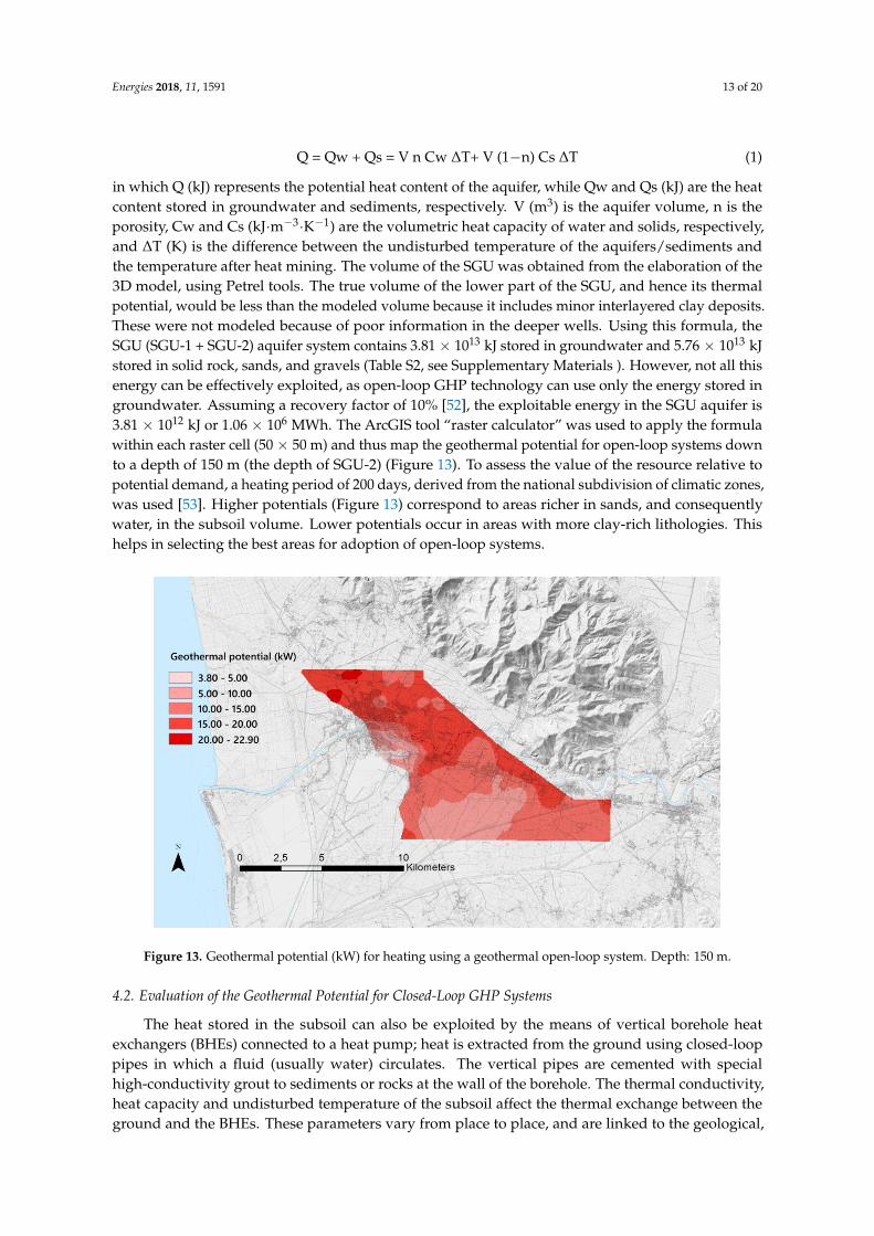
in which Q (kJ) represents the potential heat content of the aquifer, while Qw and Qs (kJ) are the heatcontent stored in groundwater and sediments, respectively. V (m3) is the aquifer volume, n is theporosity, Cw and Cs (kJ·m−3·K−1) are the volumetric heat capacity of water and solids, respectively,and ∆T (K) is the difference between the undisturbed temperature of the aquifers/sediments andthe temperature after heat mining. The volume of the SGU was obtained from the elaboration of the3D model, using Petrel tools. The true volume of the lower part of the SGU, and hence its thermalpotential, would be less than the modeled volume because it includes minor interlayered clay deposits.These were not modeled because of poor information in the deeper wells. Using this formula, theSGU (SGU-1 + SGU-2) aquifer system contains 3.81 × 1013 kJ stored in groundwater and 5.76 × 1013 kJstored in solid rock, sands, and gravels (Table S2, see Supplementary Materials ). However, not all thisenergy can be effectively exploited, as open-loop GHP technology can use only the energy stored ingroundwater. Assuming a recovery factor of 10% [52], the exploitable energy in the SGU aquifer is3.81 × 1012 kJ or 1.06 × 106 MWh. The ArcGIS tool “raster calculator” was used to apply the formulawithin each raster cell (50 × 50 m) and thus map the geothermal potential for open-loop systems downto a depth of 150 m (the depth of SGU-2) (Figure 13). To assess the value of the resource relative topotential demand, a heating period of 200 days, derived from the national subdivision of climatic zones,was used [53]. Higher potentials (Figure 13) correspond to areas richer in sands, and consequentlywater, in the subsoil volume. Lower potentials occur in areas with more clay-rich lithologies. Thishelps in selecting the best areas for adoption of open-loop systems.

Energies 2018, 11, x FOR PEER REVIEW 13 of 20

The heat stored in the phreatic or confined aquifers may be mined through doublets of wells

(both production and reinjection wells) and a heat exchanger that represents the interface with the

heat pump. This type of assemblage allows heat to be sustainably mined, without any loss or

contamination of water, because all the water from the production well is reinjected restoring the

hydraulic capacities of the aquifer.

The geothermal potential of the aquifers of the Pisa plain subsoil can then be estimated using

the volumetric method equation [23,24]:

Q = Qw + Qs = V n Cw ΔT+ V (1–n) Cs ΔT (1)

in which Q (kJ) represents the potential heat content of the aquifer, while Qw and Qs (kJ) are the heat

content stored in groundwater and sediments, respectively. V (m3) is the aquifer volume, n is the

porosity, Cw and Cs (kJ·m−3·K−1) are the volumetric heat capacity of water and solids, respectively,

and ΔT (K) is the difference between the undisturbed temperature of the aquifers/sediments and the

temperature after heat mining. The volume of the SGU was obtained from the elaboration of the 3D

model, using Petrel tools. The true volume of the lower part of the SGU, and hence its thermal

potential, would be less than the modeled volume because it includes minor interlayered clay

deposits. These were not modeled because of poor information in the deeper wells. Using this

formula, the SGU (SGU-1 + SGU-2) aquifer system contains 3.81 × 1013 kJ stored in groundwater and

5.76 × 1013 kJ stored in solid rock, sands, and gravels (Table s2, see Supplementary Materials ).

However, not all this energy can be effectively exploited, as open-loop GHP technology can use only

the energy stored in groundwater. Assuming a recovery factor of 10% [52], the exploitable energy in

the SGU aquifer is 3.81 × 1012 kJ or 1.06 × 106 MWh. The ArcGIS tool “raster calculator” was used to

apply the formula within each raster cell (50 × 50 m) and thus map the geothermal potential for open-

loop systems down to a depth of 150 m (the depth of SGU-2) (Figure 13). To assess the value of the

resource relative to potential demand, a heating period of 200 days, derived from the national

subdivision of climatic zones, was used [53]. Higher potentials (Figure 13) correspond to areas richer

in sands, and consequently water, in the subsoil volume. Lower potentials occur in areas with more

clay-rich lithologies. This helps in selecting the best areas for adoption of open-loop systems.

Figure 13. Geothermal potential (kW) for heating using a geothermal open-loop system. Depth: 150

m.

4.2. Evaluation of the Geothermal Potential for Closed-Loop GHP Systems

Figure 13. Geothermal potential (kW) for heating using a geothermal open-loop system. Depth: 150 m.

4.2. Evaluation of the Geothermal Potential for Closed-Loop GHP Systems

The heat stored in the subsoil can also be exploited by the means of vertical borehole heatexchangers (BHEs) connected to a heat pump; heat is extracted from the ground using closed-looppipes in which a fluid (usually water) circulates. The vertical pipes are cemented with specialhigh-conductivity grout to sediments or rocks at the wall of the borehole. The thermal conductivity,heat capacity and undisturbed temperature of the subsoil affect the thermal exchange between theground and the BHEs. These parameters vary from place to place, and are linked to the geological,

Energies 2018, 11, 1591 14 of 20

hydrogeological and geothermal settings of the site where the system is installed. An accurateknowledge of these parameters is fundamental for correct dimensioning of the system. The numberand length of BHEs required for the closed-loop system depends on the thermal characteristics of thesubsurface and on the required heating (or cooling) capacity.

Evaluation of the geothermal potential of closed-loop systems is commonly based on specificsoftware (i.e., EED, Earth Energy Designer) or tabular data [54]. In this work, the geothermal potentialof closed-loop systems was evaluated applying the “G.POT” (Geothermal POTential) method [55].As above, we considered a heating period of 200 days [53].

Ground thermal properties were derived from the numerical simulation and the literature.The ground thermal conductivity (W·m−1·K−1) was depth-averaged over the first 100 meters, whichrepresents the average length of BHEs (Figure 14).

Energies 2018, 11, x FOR PEER REVIEW 14 of 20

The heat stored in the subsoil can also be exploited by the means of vertical borehole heat

exchangers (BHEs) connected to a heat pump; heat is extracted from the ground using closed-loop

pipes in which a fluid (usually water) circulates. The vertical pipes are cemented with special high-

conductivity grout to sediments or rocks at the wall of the borehole. The thermal conductivity, heat

capacity and undisturbed temperature of the subsoil affect the thermal exchange between the ground

and the BHEs. These parameters vary from place to place, and are linked to the geological,

hydrogeological and geothermal settings of the site where the system is installed. An accurate

knowledge of these parameters is fundamental for correct dimensioning of the system. The number

and length of BHEs required for the closed-loop system depends on the thermal characteristics of the

subsurface and on the required heating (or cooling) capacity.

Evaluation of the geothermal potential of closed-loop systems is commonly based on specific

software (i.e., EED, Earth Energy Designer) or tabular data [54]. In this work, the geothermal potential

of closed-loop systems was evaluated applying the “G.POT” (Geothermal POTential) method [55].

As above, we considered a heating period of 200 days [53].

Ground thermal properties were derived from the numerical simulation and the literature. The

ground thermal conductivity (W·m–1·K–1) was depth-averaged over the first 100 meters, which

represents the average length of BHEs (Figure 14).

Figure 14. Thermal conductivity map (W m-1·K–1), weighed average over 100 m depth.

The mapping used the thermal conductivity values and thicknesses of alluvial deposits adopted

for the numerical simulation. For the mostly clayey sediments a value of 1.8 W m–1 K–1 was used,

while for the mostly sandy aquifer a value of 2 W·m–1·K–1 was assigned. Horizontal variations in

thermal conductivity are linked to different thicknesses of clayey and sandy sediments. The highest

values of thermal conductivity occur in areas where clay sediments are subordinate to the sandy

aquifer. The temperature distribution (°C) at 50 m depth (Figure 12b) derived from the numerical

simulation was used as the undisturbed temperature of the ground. Assuming a BHE length of 100

m, the temperature at 50 m depth can be adopted as the mean temperature along the pipe. Volume-

related specific heat capacity values were derived from guidelines [54]: a value of 2.5 MJ·m–3·K–1 was

used.

A standard vertical BHE was used, according to prior methodology [55], for evaluation of the

geothermal potential throughout the area. The parameters for this BHE, needed for the calculation of

borehole thermal resistance and heat transfer with the ground, are listed in Table s3 (see

Supplementary Materials).

Figure 14. Thermal conductivity map (W·m−1·K−1), weighed average over 100 m depth.

The mapping used the thermal conductivity values and thicknesses of alluvial deposits adoptedfor the numerical simulation. For the mostly clayey sediments a value of 1.8 W·m−1·K−1 was used,while for the mostly sandy aquifer a value of 2 W·m−1·K−1 was assigned. Horizontal variations inthermal conductivity are linked to different thicknesses of clayey and sandy sediments. The highestvalues of thermal conductivity occur in areas where clay sediments are subordinate to the sandyaquifer. The temperature distribution (◦C) at 50 m depth (Figure 12b) derived from the numericalsimulation was used as the undisturbed temperature of the ground. Assuming a BHE length of 100 m,the temperature at 50 m depth can be adopted as the mean temperature along the pipe. Volume-relatedspecific heat capacity values were derived from guidelines [54]: a value of 2.5 MJ·m−3·K−1 was used.

A standard vertical BHE was used, according to prior methodology [55], for evaluation of thegeothermal potential throughout the area. The parameters for this BHE, needed for the calculationof borehole thermal resistance and heat transfer with the ground, are listed in Table S3 (seeSupplementary Materials).

Figure 15 shows the distribution of geothermal potential, for single standard vertical BHE,based on the use of closed-loop technology. Comparing the calculated kW values with the thermalconductivity (Figure 14) and undisturbed temperature of the ground (Figure 12b), it is immediatelyclear that the highest thermal potential (4.75 kW) occurs in the areas of highest thermal conductivityand temperature. The highest temperature values are indicated as being north of the Arno river.

Energies 2018, 11, 1591 15 of 20

The whole investigated area is very promising for the installation of closed-loop systems, since from asingle vertical BHE, between 3.5 and 4.75 kW can be extracted for heating purposes. Generally, a GHPplant would include more than 1 vertical BHE, depending on the power of the GHP and heatingrequirements of the buildings.

Energies 2018, 11, x FOR PEER REVIEW 15 of 20

Figure 15 shows the distribution of geothermal potential, for single standard vertical BHE, based

on the use of closed-loop technology. Comparing the calculated kW values with the thermal

conductivity (Figure 14) and undisturbed temperature of the ground (Figure 12b), it is immediately

clear that the highest thermal potential (4.75 kW) occurs in the areas of highest thermal conductivity

and temperature. The highest temperature values are indicated as being north of the Arno river. The

whole investigated area is very promising for the installation of closed-loop systems, since from a

single vertical BHE, between 3.5 and 4.75 kW can be extracted for heating purposes. Generally, a GHP

plant would include more than 1 vertical BHE, depending on the power of the GHP and heating

requirements of the buildings.

Figure 15. Geothermal potential (kW) for heating-only by geothermal closed-loop systems (for 1

standard vertical BHE). Depth: 100 m. The calculation follows [46] QBHE = [a (T0 − Tlim) λ L

t’c]/[−0.619 t’c log (u’s) + (0.532 t’c − 0.962) log (u’c) − 0.455 t’c − 1.619 + πλRb]; where QBHE (MWh/y)

is the geothermal potential for a standard vertical BHE for heating only, a = 0.0701, T0 is the ground

undisturbed temperature, Tlim is the minimum temperature of the heat carrier fluid, λ is the ground

thermal conductivity, L is the length of the pipes, t’c = tc/365 where tc is the heating period, Rb is the

borehole thermal resistance, u’s = rb2/(4αts) and u’c = rb2/(4αtc) where rb is the borehole radius, α =

λ/ρc is the thermal diffusivity of the ground and ts is the operating time of the system. For a more

practice use, we derived kW values from the calculated MWh/y.

4.3. Evaluation of the Geothermal Potential for the Bedrock

As previously stated, the temperatures in bedrock range between 40° and 90 °C at depths from

500 m to 1400 m bgl. The bedrock is formed by carbonate formations, possibly hosting thermal fluids.

These fluids may be utilized directly or increasing their temperature (before using fluids) through

GHP or other technologies, in GeoDH plants.

The evaluation of this type of geothermal resource, deeper and hotter than those described above,

was performed using the volumetric method [23,24] and the reconstructed bedrock unit. For

economic reasons (well drilling cost), the calculation was limited to the area where carbonate

formations hosting thermal waters are relatively shallow (<600 m, structural high of the bedrock. The

volume, over an area of 53 km2, assuming a constant thickness of 200 m, is 10.6 km3. The parameters

used for the bedrock geothermal potential calculation are summarized in Table s4 (see

Figure 15. Geothermal potential (kW) for heating-only by geothermal closed-loop systems (for1 standard vertical BHE). Depth: 100 m. The calculation follows [46] QBHE = [a (T0 − Tlim) λ Lt’c]/[−0.619 t’c log (u’s) + (0.532 t’c − 0.962) log (u’c) − 0.455 t’c − 1.619 + πλRb]; where QBHE(MWh/y) is the geothermal potential for a standard vertical BHE for heating only, a = 0.0701, T0 is theground undisturbed temperature, Tlim is the minimum temperature of the heat carrier fluid, λ is theground thermal conductivity, L is the length of the pipes, t’c = tc/365 where tc is the heating period, Rbis the borehole thermal resistance, u’s = rb2/(4αts) and u’c = rb2/(4αtc) where rb is the borehole radius,α = λ/ρc is the thermal diffusivity of the ground and ts is the operating time of the system. For a morepractice use, we derived kW values from the calculated MWh/y.

4.3. Evaluation of the Geothermal Potential for the Bedrock

As previously stated, the temperatures in bedrock range between 40◦ and 90 ◦C at depths from500 m to 1400 m bgl. The bedrock is formed by carbonate formations, possibly hosting thermal fluids.These fluids may be utilized directly or increasing their temperature (before using fluids) throughGHP or other technologies, in GeoDH plants.

The evaluation of this type of geothermal resource, deeper and hotter than those described above,was performed using the volumetric method [23,24] and the reconstructed bedrock unit. For economicreasons (well drilling cost), the calculation was limited to the area where carbonate formations hostingthermal waters are relatively shallow (<600 m, structural high of the bedrock. The volume, over anarea of 53 km2, assuming a constant thickness of 200 m, is 10.6 km3. The parameters used for thebedrock geothermal potential calculation are summarized in Table S4 (see Supplementary Materials).The geothermal energy potential contained within the first 200 m of the bedrock, limited to the area ofgravimetric structural high, is equal to 8.30 × 1014 kJ, or 2.31 × 108 MWh.

Energies 2018, 11, 1591 16 of 20

Except for information from the S. Cataldo 1 and Poggio 1 deep wells, no data regarding the natureand permeability of the bedrock lithologies are available. Consequently, the calculated geothermalpotential is to be considered only as approximate guidance.

4.4. Sustainability

The detailed 3D thermofluidodynamic modeling of subsoil defined by the steady-state conditionsof the simulated volume (Figures 8 and 9), represents a snapshot of the Pisa plain system beforeany geothermal utilization. This is the undisturbed situation but would be affected by heat mining.To determine the level of sustainable use of the resource, it would be appropriate to undertake dynamicmodeling, inserting in the 3D model and simulator shallow or deep doublets of wells or vertical BHE,and hence determine the impact on the subsoil resource of GHP and GeoDH exploitation. This wouldbe an important result because it provides a means of regulating application of these technologies toavoid environmental impacts on the subsoil thermal state or on the water resource.

5. Conclusions

This paper demonstrates a methodology for assessment of renewable geothermal resources,based on the collection, storage, interpretation, and visualization of a large volume of data in a 3Denvironment, allowing optimal use of such information.

Application of this methodology to the alluvial-sedimentary geological environment of the Pisaplain, indicates that geological modelling and geothermal numerical simulations, can provide data onthe amount of energy that shallow geothermal resources (sediments, rocks, and water) can furnish,including evaluation of the local shallow geothermal (low temperature) potential for GHP (openor closed loop systems) or for wider area heat mining from deeper and hotter geothermal aquifers.The study area was found to have high geothermal potential: the heat stored in water and rocks, up to150 m depth, is about 2.5 × 107 MWh. Thematic maps provided spatially explicit estimation of thegeothermal potential of different heat exchange technologies, supporting the optimal design of heatingand cooling plants.

Low-temperature geothermal resources are ubiquitous in the shallow earth crust, making ourapproach (as exemplified in the case study) widely replicable. The approach produces informationabout local geothermal resources, guiding low temperature geothermal plant designers, geologists,and engineers, towards the most efficient solution for a specific site. In particular, knowledge of subsoilgeology, derived from 3D reconstruction and a well-geodatabase, can facilitate the diffusion of GHPtechnology by supporting site selection and drilling of well doublets (for GHP open-loop systems) orvertical heat exchangers (for GHP closed-loop systems).

The methodology not only identifies favorable locations for a specific exchange technology,but also provides a robust conceptual model of the subsoil and supports the thermofluidodynamicmodeling necessary for design of sustainable plants that preserve the thermal state of subsoil over thelong-term. This approach can ensure environmental sustainability through best practice in the designand regulation of GHP and GeoDH systems, with their attendant environmental benefits.

Supplementary Materials: The following are available online at http://www.mdpi.com/1996-1073/11/6/1591/s1, Table S1: Initial conditions and parameters for TOUGH2 simulation, Table S2: Geothermal energy calculation(Balke, 1977, Muffler and Cataldi, 1978), Table S3: Parameters for the standard vertical BHE, Table S4: Bedrockgeothermal potential calculation (Balke, 1977, Muffler and Cataldi, 1978).

Author Contributions: Conceptualization, A.S. and P.M.; Methodology, A.S., P.M. and G.P.; Validation, P.M.;Formal Analysis, P.C., F.P., V.C., M.S. and G.P.; Investigation, G.P. and F.P.; Resources, P.C.; Software, P.C. and G.P.;Data Curation, G.P.; Writing—Original Draft Preparation, P.M., G.P. and A.S.; Writing—Review & Editing, A.S.,P.M., P.C., G.P., F.P., V.C. and M.S.; Visualization, G.P., V.C., P.C., F.P; Supervision, A.S.; Project Administration,A.S.; Funding Acquisition, A.S.

Funding: This work was financially supported by “Geo4P” project (EnerGea, CoSviG and Regional Governmentof Tuscany) and University of Pisa, grant to A. Sbrana.

Energies 2018, 11, 1591 17 of 20

Acknowledgments: L. Paci is acknowledged for the technical support during the starting phase of the project.L. Torsello and D. Bonciani are acknowledged for discussion and support during the activity of Geo4P project.Acque SpA and the Civil Engineer division of the Regional Government of Tuscany are acknowledged for sharingtheir water well data base. The authors are grateful to two anonymous reviewers for their constructive commentsand suggestions that helped to improve the quality of the manuscript

Conflicts of Interest: The authors declare no conflict of interest.

Abbreviations

The following abbreviations are used in this manuscript:

2D Two-dimensional3D Three-dimensionala.s.l Above Sea Levelbgl Below Ground LevelBHE Borehole Heat ExchangerCDU Coastal Dune UnitCU Clay UnitCSU Clay and Sands UnitDTM Digital Terrain ModelEED Earth Energy DesignerEPSG European Petroleum Survey GroupGeoDH Geothermal District Heating systemsGFU Gravel Fans UnitGHP Geothermal Heat PumpGIS Geographic Information SystemGRS Geodetic Reference SystemG.POT Geothermal POTential methodIDW Inverse Distance Weighted interpolationIFD Integral Finite DifferenceRAC Recent Alluvial CoverSGU Sands and Gravels UnitSGU-1 Sands and Gravels upper UnitSGU-2 Sands and Gravels lower UnitTOUGH Transport of Unsaturated Groundwater and HeatEOS Equation of StateUTM Universal Transverse of Mercator, cartographic projectionWGS World Geodetic System

References

1. De la Cruz-Lovera, C.; Perea-Moreno, A.J.; de la Cruz-Fernández, J.L.; Alvarez-Bermejo, J.A.; Manzano-Agugliaro, F. Worldwide Research on Energy Efficiency and Sustainability in Public Buildings. Sustainability2017, 9, 1294. [CrossRef]

2. Pérez-Lombard, L.; Ortiz, J.; Pout, C. A review on buildings energy consumption information. Energy Build.2008, 40, 394–398. [CrossRef]

3. EU. Directive 2010/31/EU of the European Parliament and of the Council of 19 May 2010 on the EnergyPerformance of Buildings. Available online: http://eur-lex.europa.eu/legal-content/en/TXT/?uri=CELEX(accessed on 2 June 2018).

4. Harvey, C.; Beardsmore, G.; Moeck, I.; Rüter, H. Geothermal Exploration: Global Strategies and Applications; IGAService GmbH: Bochum, Germany, 2016.

5. Chesnaux, R.; Lambert, M.; Fillastre, U.; Walter, J.; Hay, M.; Rouleau, A.; Daigneault, R.; Germaneau, D.;Moisan, A. Building a geodatabase for mapping hydrogeological features and 3D modeling of groundwatersystems: Application to the Saguenay-Lac-St-Jean Region, Canada. Comput. Geosci. 2001, 37, 1870–1882.[CrossRef]

Energies 2018, 11, 1591 18 of 20

6. Gogu, R.; Carabin, G.; Hallet, V.; Peters, V.; Dassargues, A. GIS-based hydrogeological databases andgroundwater modeling. Hydrogeol. J. 2001, 9, 555–569. [CrossRef]

7. Kaufmann, O.; Martin, T. 3D geological modeling from boreholes, cross-sections and geological maps,application over former natural gas storages in coal mines. Comput. Geosci. 2008, 34, 278–290. [CrossRef]

8. Noorollahi, Y.; Itoi, R.; Fujii, H.; Tanaka, T. GIS integration model for geothermal exploration and well siting.Geothermics 2008, 37, 107–131. [CrossRef]

9. Schiel, K.; Baume, O.; Caruso, G.; Leopold, U. GIS-based modelling of shallow geothermal energy potentialfor CO2 emission mitigation in urban areas. Renew. Energy 2016, 86, 1023–1036. [CrossRef]

10. Ondreka, J.; Rusgen, M.I.; Stober, I.; Czurda, K. GIS-supported mapping of shallow geothermal potentialof representative areas in south-western Germany—Possibilities and limitations. Renew. Energy 2007, 32,2186–2200. [CrossRef]

11. Akar, S.; Atalay, O.; Kuyumcu, O.C.; Solaroglu, U.Z.D.; Colpan, B.; Arzuman, S. 3D subsurface modeling ofGumuscoy Geothermal Area, Aydin, Turkey. Geotherm. Resour. Counc. Trans. 2011, 35, 669–676.

12. Alkaraz, S.; Lane, R.; Spragg, K.; Milicich, S.; Sepulveda, F.; Bignall, G. 3D Geological Modelling Using NewLeapfrog Geothermal Software. In Proceedings of the 36th Workshop on Geothermal Reservoir Engineering,Stanford University, Stanford, CA, USA, 31 January 31–2 February 2011.

13. Alkaraz, S.; Chamberfort, I.; Pearson, R.; Cantwell, A. An Integrated Approach to 3-D Modelling toBetter Understand Geothermal Reservoirs. In Proceedings of the World Geothermal Congress, Melbourne,Australia, 19–25 April 2015; pp. 1–7.

14. Pearson, S.C.P.; Alcaraz, S.A.; White, P.A.; Tschritter, C. Improved visualization of reservoir simulations:Geological and fluid flow modeling of the Tauranga low-enthalpy geothermal system, New Zealand.Geotherm. Resour. Counc. Trans. 2012, 36, 1293–1297.

15. Fulignati, P.; Marianelli, P.; Sbrana, A.; Ciani, V. 3D geothermal modelling of the Mount Amiata hydrothermalsystem in Italy. Energies 2014, 7, 7434–7553. [CrossRef]

16. Bellani, S.; Grassi, S.; Squarci, P. Geothermal Characteristics of the Pisa Plain, Italy. In Proceedings of theWorld Geothermal Congress, Florence, Italy, 18–31 May 1995; Volume 2, pp. 1305–1308.

17. Feng, G.; Xu, T.; Gherardi, F.; Jiang, Z.; Bellani, S. Geothermal assessment of the Pisa plain, Italy: Coupledthermal and hydraulic modeling. Renew. Energy 2017, 111, 416–427. [CrossRef]

18. Gunnarsson, N. 3D Modeling in Petrel of Geological CO2 Storage Site. Master’s Thesis, Uppsala University,Uppsala, Sweden, 2011.

19. Pruess, K.; Oldenburg, C.; Moridis, G. TOUGH2 User’s Guide, Version 2.0. Report LBNL-43134; LawrenceLivermore Laboratory: Berkeley, CA, USA, 1999; 198p.

20. Narasimhan, T.N.; Witherspoon, P.A. An integrated finite difference method for analyzing fluid flow inporous media. Water Resour. Res. 1976, 12, 57–64. [CrossRef]

21. Audigane, P.; Chiaberge, C.; Mathurin, F.; Lions, J.; Picot-Colbeaux, G. A workflow for handlingheterogeneous 3D models with the TOUGH2 family of codes: Application to numerical modeling ofCO2 geological storage. Comput. Geosci. 2011, 37, 610–620. [CrossRef]

22. Shepard, D. A Two-Dimensional Interpolation Function for Irregularly-Spaced Data. In Proceedings of the1968 ACM National Conference, New York, NY, USA, 27–29 August 1968; pp. 517–524.

23. Balke, K.-D. Das Grundwasser als Energieträger. Brennstoff-Warme-Kraft 1977, 29, 191–194.24. Muffler, P.; Cataldi, R. Methods for regional assessment of geothermal resources. Geothermics 1978, 7, 53–89.

[CrossRef]25. Pascucci, V.; Fontanesi, G.; Merlini, S.; Martini, I.P. Neogene Tuscan Shelf-Western Tuscany extension:

Evidences of the early post-compressional deposits (Tyrrhenian Sea-Northern Apennines, Italy). Ofioliti 2001,26, 187–196. [CrossRef]

26. Sarti, G.; Rossi, V.; Giacomelli, S. The upper Pleistocene “Isola di Coltano sands” (Arno coastal plain, TuscanyItaly): Review of stratigraphic data and tectonic implications for the southern margin of the Viareggio basin.Atti Soc. Tosc. Sci. Nat. Mem. Pisa Italy Serie A 2015, 122, 75–84.

27. Mariani, M.; Prato, R. I bacini neogenici costieri del margine tirrenico: Approccio sismico-stratigrafico.Mem. Soc. Geol. Ital. 1988, 41, 519–531. (In Italian)

28. Trevisan, L.; Tongiorgi, E. Le Acque del Sottosuolo della Regione Pisana. “La Provincia Pisana”; AmministrazioneProvinciale: Pisa, Italy, 1953; pp. 3–8. (In Italian)

Energies 2018, 11, 1591 19 of 20

29. Dini, I. La Prima Falda Artesiana in Sabbia della Zona di Pisa; Comune e Provincia di Pisa: Pisa, Italy, 1976.(In Italian)

30. Tongiorgi, M.; Rau, A.; Martini, I.P. Sedimentology of early-alpine, fluvio-marine, clastic deposits (Verrucano,Triassic) in the Monti Pisani (Italy). Sediment. Geol. 1997, 17, 311–332. [CrossRef]

31. Fancelli, R. Tentativo di Ricostruzione Dell’andamento della Falda Artesiana tra i-30 ed i-50 m di Profondità nelSottosuolo di Pisa e Dintorni; Rapporto CNR; Istituto Internazionale Ricerche Geotermiche: Pisa, Italy, 1984.(In Italian)

32. Fancelli, R. Alcune Notizie sui Sedimenti Attraversati da Perforazioni per Ricerche D’acqua e Sulla DistribuzioneSpaziale nel Sottosuolo Pisano delle Falde Acquifere; Rapporto CNR; Istituto Internazionale Ricerche Geotermiche:Pisa, Italy, 1984. (In Italian)

33. Baldacci, F.; Bellini, L.; Raggi, G. Le risorse idriche sotterranee della pianura pisana. Atti Soc. Tosc. Sci. Nat.Mem. Pisa Italy Serie A 1994, 101, 241–322. (In Italian)

34. Rossi, S.; Spandre, R. Caratteristiche idrochimiche della I falda artesiana in sabbia nei dintorni della città diPisa. Acque sotterr. Fasc. 1994, 43, 51–58. (In Italian)

35. Aguzzi, M.; Amorosi, A.; Sarti, G. Stratigraphic architecture of late quaternary deposits in the lower Arnoplain (Tuscany, Italy). Geol. Romana 2005, 38, 1–10.

36. Aguzzi, M.; Amorosi, A.; Castorina, F.; Ricci Lucchi, M.; Sarti, G.; Vaiani, C. Stratigraphic architecture andaquifer systems in the eastern Valdarno Basin, Tuscany. Geoacta 2006, 5, 39–60.

37. Aguzzi, M.; Amorosi, A.; Colalongo, M.L.; Ricci Lucchi, M.; Rossi, V.; Sarti, G.; Vaiani, S.C. Late Quaternaryclimatic evolution of the Arno coastal plain (Western Tuscany, Italy) from subsurface data. Sediment. Geol.2007, 202, 211–229. [CrossRef]

38. Grassi, S.; Cortecci, G. Hydrogeology and geochemistry of the multi-layered confined aquifer of the Pisaplain (Tuscany-central Italy). Appl. Geochem. 2005, 20, 41–54. [CrossRef]

39. Amorosi, A.; Lucchi, M.R.; Rossi, V.; Sarti, G. Climate change signature of small-scale parasequences fromlate glacial-Holocene transgressive deposits of the Arno valley fill. Paleogeogr. Paleoclimatol. Palaeoecol. 2009,273, 142–152. [CrossRef]

40. Sarti, G.; Rossi, V.; Amorosi, A. Influence of Holocene stratigraphic architecture on ground surfacesettlements: A case study from City of Pisa (Tuscany, Italy). Sediment. Geol. 2012, 281, 75–87. [CrossRef]

41. Bonham-Carter, G.F. Geographic Information Systems for Geoscientists: Modeling with GIS; Pergamon Press:Oxford, UK, 1994; 398p.

42. Carratori, L.; Ceccarelli Lemut, M.L.; Frattarelli Fischer, L.; Garzella, G.; Greco, G.; Grifoni Cremonesi, R.;Mazzanti, R.; Morelli, P.; Nencini, C.; Pasquinucci, M.; et al. Carta degli elementi naturalistici e storici dellaPianura di Pisa e dei rilievi contermini, scala 1:50.000. In La Pianura di Pisa e i Rilievi Contermini la Natura e laStoria; Mazzanti, R., Ed.; Memorie della Società Geografica Italiana L: Rome, Italy, 1994; 491p. (In Italian)

43. Belgiorno, M.; Marianelli, P.; Pasquini, G.; Sbrana, A. A contribution to the study of a Pisa alluvial plainsector for low-temperature geothermal assessment. Atti Soc. Tosc. Sci. Nat. Mem. Pisa Italy 2016, 123, 17–23.[CrossRef]

44. Sbrana, A.; Pasquini, G.; Marianelli, P.; Bonciani, D.; Torsello, L. Geo4P-Geothermal Pilot Project PisanPlain: Quantitative assessment of very low, low and medium temperature shallow geothermal resources.In Proceedings of the European Geothermal Congress, Technology and Best practice—Exploration andPlanning, Strasbourg, France, 19–24 September 2016.

45. Hinze, W.J.; Aiken, C.; Brozena, J.; Coakley, B.; Dater, D.; Flanagan, G.; Forsberg, R.; Hildenbrand, T.;Keller, G.R.; Kellogg, J.; et al. New standards for reducing gravity data: The North America gravity database.Geophysics 2005, 70, J25–J32. [CrossRef]

46. Moritz, H. Geodetic Reference System 1980. Bull. Géod. 1980, 54, 395–405. [CrossRef]47. Banerjee, B.; Das Gupta, S.P. Gravitational attraction of a rectangular parallelepiped. Geophysics 1977, 42,

1053–1055. [CrossRef]48. Bott, M.H.P. The use of rapid digital computing methods for direct gravity interpretation of sedimentary

basins. Geophys. J. Int. 1960, 3, 63–67. [CrossRef]49. Tuscany Region Website. Available online: http://www.regione.toscana.it/-/geoscopio (accessed on

14 May 2018).50. Hydrogeological Sector, Tuscany Region. Available online: http://www.sir.toscana.it (accessed on

14 May 2018).

Energies 2018, 11, 1591 20 of 20

51. Zhu, K.; Blum, P.; Ferguson, G.; Balke, K.-D.; Bayer, P. The geothermal potential of urban heat islands.Environ. Res. Lett. 2010, 5, 044002. [CrossRef]

52. Hurter, S.; Huenges, E.; Clauser, C.; Haenel, R. (Eds.) Atlas of Geothermal Resources in Europe; EuropeanCommission Office for Official Publications of the European Communities: Brussels, Belgium, 2002; 93p.

53. Gazzetta Ufficiale della Repubblica Italiana, D.P.R. 142/93, Allegato A. Available online: http://efficienzaenergetica.acs.enea.it/doc/dpr412-93.pdf (accessed on 14 May 2018). (In Italian)

54. VDI. VDI 4640 Thermal Use of the Underground. Blatt 1: Fundamentals, Approvals, Environmental Aspects; VDI:Düsseldorf, Germany, 2010.

55. Casasso, A.; Sethi, R. G.POT: A quantitative method for the assessment and mapping of the shallowgeothermal potential. Energy 2016, 106, 765–773. [CrossRef]

© 2018 by the authors. Licensee MDPI, Basel, Switzerland. This article is an open accessarticle distributed under the terms and conditions of the Creative Commons Attribution(CC BY) license (http://creativecommons.org/licenses/by/4.0/).