WORKING PAPER: COMMENTS WELCOME

The Insurance Value of Medical Innovation*

Darius Lakdawalla University of Southern California and NBER

Anup Malani

University of Chicago and NBER

Julian Reif University of Illinois at Urbana-Champaign

Abstract. New, expensive medical technologies are often viewed as a major source of financial risk that heighten the value of health insurance. While true in a static sense, this viewpoint overlooks the manner in which medical innovations reduce health risks borne by consumers. Conventional economic approaches to valuing medical technology tend to ignore this “insurance value” of medical technology, and instead to assume that health risks are either absent or costless for consumers to bear. We present an alternative and more general framework that incorporates both price risk and health risk-reduction into the value of new medical technologies. Using data from the Tufts Cost-Effectiveness Registry on a range of medical technologies, we estimate that the total insurance value on average adds about 100% to the traditional valuation of medical technology. Moreover, for typical levels of risk aversion, the insurance value of technology is many times larger than the insurance value of health insurance itself. Our findings also suggest standard methods disproportionately undervalue treatments for severe illnesses, where risk to consumers is most costly, compared to milder conditions where risks are less costly to bear.

* We are grateful to Marika Cabral, Amitabh Chandra, Heidi Williams, and participants at the 2014 American Economic Association meetings, the 2014 ASHEcon meeting, Harvard Medical School, Harvard Law School, the Indiana University Health Economics Workshop, the NBER Joint Healthcare and Insurance Program meeting, the NBER Health Economics Program meeting, the Pritzker School of Medicine, the University of Chicago Applications workshop, the University of Chicago Health Economics Workshop, the University of Illinois CBPP seminar series, UCSB, and USC for helpful comments. Charles Zhang provided outstanding research assistance.

1

I. INTRODUCTION Medical innovation is frequently pinpointed as a primary driver for the rising cost of health insurance (Altman and Blendon 1977, LaCronique and Sandier 1981, Showstack, Stone et al. 1985, Wilensky 1990, Newhouse 1992, Zweifel, Felder et al. 1999, Okunade and Murthy 2002, Chandra and Skinner 2012). As a result, health policymakers often think about innovation as expanding the total quantity of risk that must be insured within the healthcare system (Weisbrod 1991). This view is not quite right. Although expensive medical technologies do pose financial risks, the effective ones also reduce physical risks from illness (Philipson and Zanjani 2013). If the latter effect exceeds the former, the technology may be welfare-enhancing. This paper provides a framework with which to evaluate therapeutic medical technologies accounting for both types of risk and quantify their welfare impacts.

The leading method by which insurance companies and government payers, as well as economists, value new medical technologies is cost-effectiveness analysis. Although it comes in many flavors, cost-effectiveness analysis fails to captures either the increase in financial risk or reduction in health risk due to technologies because it evaluates them from an ex post perspective. The reason is that cost-effectiveness analysis seeks to determine whether a new treatment makes it less costly to live with an illness for patients currently with that illness. However, it does not attempt to determine whether the new treatment also makes it less costly to face the risk of acquiring that illness in the future for patients without the illness.

To illustrate the importance of separately valuing such risk-reduction, consider a consumer who faces a “coin-toss” gamble that yields a loss of $1000 on heads, and $0 on tails, with an expected loss of $500. If a firm offers a product that replaces this gamble with a loss of $400 for sure, the expected value of this product is $100. However, a risk-averse consumer would surely pay more than $100 for it. Supposing the risk-averse consumer is willing to pay $175 for the product, we can say the expected value of the product is $100 but the incremental “insurance value” is $75. When it comes to valuing new health technologies, the standard practice in economics, however, has been to focus entirely on the $100 expected value, and abstract from the “insurance value” of new health technologies.(Philipson and Jena 2006, Yin, Penrod et al. 2012) Specifically, cost-effectiveness analysis estimates the value of health technology to be the expected clinical benefit of the technology (e.g., life-years gained) multiplied by the marginal value placed by consumers on each unit of benefit. The reduction in the variance of a consumer’s health outcomes is ignored, even though a risk-averse consumer likely values this reduction over and above the gain in expected outcomes.1

We can unpack the reduction in variance from new technologies into two distinct types of insurance value. First, a medical technology that is ex post cost-effective necessarily reduces the overall cost of becoming sick with the disease that it treats. This provides “self-insurance” as defined by Isaac Ehrlich and Gary Becker (1972), because it reduces the loss suffered in the sick state.2 Second, because real-world health insurance contracts cover the cost of medical treatments rather than the cost of illness itself, new medical technologies expand the ability of financial markets to transfer resources from the healthy state to the sick state. In other words, medical technology expands possibilities for “market insurance” as defined by Ehrlich and Becker (1972). Both these sources of value accrue above and beyond the standard notion of consumer surplus that would accrue if medical technology functioned like other goods without risky demands. To connect these two insurance concepts to what health policymakers are really complaining about when they criticize the high

1 This simplification would not matter so much in a world with perfect, pure indemnity health insurance that eliminated the financial cost of bearing healthcare risks. In our example, this would correspond to a contract that swapped the coin-toss gamble for a sure payment of $500. However, real-world health insurance markets operate far from this ideal of perfect indemnity insurance. In a world of incomplete insurance contracts, new medical treatments that reduce health risks may provide non-trivial insurance value to consumers.

2 An analogy from Ehrlich and Becker (1972) is a sprinkler system that reduces the loss from a fire.

2

price of and thus financial risk from an innovation, note that a high price of medical technology implies a low self-insurance value of innovation. However, a high price also implies a large market insurance value from innovation, so long as the innovation generates more consumer surplus than substitutes.

A medical example clarifies the self-insurance and market-insurance value of innovation. Think of a healthy consumer facing the risk of developing Parkinson’s disease3 in the years before the discovery of effective dopamine-related treatments that reduce disease symptoms. In the absence of a treatment, contracting Parkinson’s might reduce her quality of life on a 0 to 1 scale from .8 to .4. The consumer could not insure herself against this risk, because real-world insurers did not (and do not) sell pure indemnity insurance contracts that make payments to consumers conditional on the occurrence of illness alone. Moreover, healthcare insurance was a poor substitute, because there were no effective treatments to cover. As a result, this consumer had to bear the full risk of Parkinson’s related symptoms herself.

Now consider the introduction of a new technology like Levodopa. Before Levodopa, Parkinson’s patients stood to lose 50% of their quality of life. After Levodopa, however, developing Parkinson’s becomes less costly, lowering quality of life from 0.8 to only 0.7. Notice how Levodopa’s introduction compresses the variance in the quality of life between the Parkinson’s and non-Parkinson’s states. This compression is valuable to consumers who dislike risk. In addition, the advent of the treatment immediately makes healthcare insurance more valuable, because there are finally effective technologies for insurance to cover. Conventional economic valuations of health technology ignore these two sources of value, but focus exclusively on the 0.3 gain in average quality of life produced.

In this paper, we provide a framework for identifying and measuring the market-insurance and self-insurance values of therapeutic innovations. 4 This has important implications for how economists value medical innovation and health insurance. First, the framework allows one to correct conventional methods for valuation by adding the insurance value of technology. This error-correction has the greatest impact when estimating the value of treatments for severe or poorly managed diseases, where risks to consumers are greatest. This finding reconciles the conventional economic approach to valuation with the findings of population surveys suggesting that people prefer to allocate resources to treating severe diseases than milder ones (Nord, Richardson et al. 1995, Green and Gerard 2009, Linley and Hughes 2013).

Second, our framework yields new insights for the relationship between financial health insurance and medical technology. The existing literature has correctly observed that health insurance can drive medical innovation (Goddeeris 1984, Newhouse 1992).5 It is also known that high-priced technology drives demand for health insurance. Thus, while the two products are price complements on the extensive margin, they are

3 Parkinson’s disease is a progressive disorder of the nervous system that degrades a patients movements. It typically manifests as a hand tremor but can also cause slowing of movement and slurring of speech, and later dementia. It’s most famous patient is the boxer Muhammad Ali. Parkinson’s symptoms can now be treated with medications such as Levodopa or MAO-B inhibitors that raise the level of dopamine in the brain.

4 In the appendix, we show that risk averse individuals also derive self-protection value from technologies that reduce the probability of events. All three components provide value to consumers above and beyond standard concepts of consumer surplus or “risk-free value,” which remain incomplete in the context of medical technology.

5 In general, health insurance is treated as an outward shift in the demand for medical technology. See, e.g., Acemoglu et al. (2006), Blume-Kohout and Sood (2008), Clemens (2012). However, Malani and Philipson (2013) also observe that health insurance can reduce the supply of human subjects for the clinical trials required for medical innovation.

3

actually price substitutes on the intensive margin of treatment.6 One the one hand, reductions in the price of technology that stimulate greater utilization also encourage greater insurance purchases (Weisbrod 1991). In contrast, lowering the price of technology for a consumer already using it also increases its self-insurance value and thus reduces the incentive to purchase formal health insurance. From a social welfare point of view, this insight also implies that medical technology has provided substantial insurance value, perhaps more than financial health insurance itself.

To illustrate the empirical significance of these results, we undertake two empirical exercises. First, we illustrate the extent to which economists, even Murphy and Topel (2006), have underestimated the benefit of new medical technologies we quantify the insurance value of quality-of-life improvements for the aggregate US population, by gender and age group, assuming these technologies have zero price. From a lifetime perspective, insurance value adds 50% to the conventional value of quality-of-life improvements for men, and 70% for women.

Second, we quantify insurance value for a sample of medical technologies studied in the Tufts Cost-Effectiveness Analysis Registry (CEAR). Specifically, we estimate for each technology (1) self-insurance value and (2) market-insurance value and then compare these to (3) standard consumer surplus value, all assuming the technologies have positive costs as reported in CEAR database studies. We find that accounting for the insurance value of therapeutic technologies more than doubles their value, on average. Moreover, for typical levels of risk aversion, the insurance value of technology is significantly larger – perhaps 20 times larger – than the insurance value of health insurance itself.

The remainder of this paper has the following outline. Section I describes the market-insurance value and the self-insurance value of therapeutic innovation to a risk-averse individual. Section II characterizes the insurance value of preventive technology that accrues to a risk-averse individual, but not a risk-neutral one. Section III provides empirical estimates of market-insurance value and self-insurance value of therapeutic technologies and compares them to the ex post consumer surplus from technology and the insurance value of health insurance. It then goes on to quantify the effect of risk aversion on the value of preventive technology.

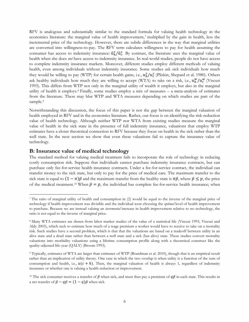
II: FRAMEWORK FOR VALUING MEDICAL TREATMENTS Consider an individual who faces a health risk. We are interested in analyzing the value of a new medical technology that treats this health risk and is cheap enough to improve consumer welfare. Thus, we focus on technologies that generate non-negative consumer surplus even in the absence of health insurance. We also focus on treatment technologies that improve health. In the appendix, we consider technologies that prevent health decline.

We first quantify the value of the treatment if the patient does not face consumption risk due to illness and the cost of medical care because she has indemnity insurance. We define this as the “risk-free value of treatment” and show that it is substantially similar to standard methods for valuing medical technology.

We then consider a more realistic environment in which indemnity insurance markets are incomplete and so consumers bear some residual financial risk due to illness. We characterize the additional self-insurance and market insurance value that accrue from medical treatments in this context. We define the sum of the two as the “insurance value of treatment” and distinguish it from the standard risk-free value.

6 Lakdawalla and Sood (2013) demonstrate that health insurance and medical innovation are complementary in the sense that health insurance reduced the static inefficiency from patents and thus reduces the cost of using patents to incentivize innovation.

4

A: The risk-free value of technology The individual derives utility from non-health consumption and from health according to 𝑢𝑢(𝑐𝑐,ℎ). She is either sick, with probability 𝜋𝜋, or well. Absent medical treatments, health is ℎ𝑤𝑤 when well and ℎ𝑠𝑠 < ℎ𝑤𝑤 when sick. The individual is endowed with income 𝑦𝑦𝑤𝑤 when well and 𝑦𝑦𝑠𝑠 ≤ 𝑦𝑦𝑤𝑤 when sick. Finally, she can purchase as much indemnity insurance as she wishes in a perfectly competitive marketplace. She can choose to transfer 𝜏𝜏 units of consumption away from the healthy state, and will receive the actuarially fair transfer [(1 − 𝜋𝜋)/𝜋𝜋]𝜏𝜏 when sick.

In the absence of medical treatment, the individual’s optimization problem is:

max𝜏𝜏

𝜋𝜋𝑢𝑢 �𝑦𝑦𝑠𝑠 +1 − 𝜋𝜋𝜋𝜋

𝜏𝜏,ℎ𝑠𝑠� + (1 − 𝜋𝜋)𝑢𝑢(𝑦𝑦𝑤𝑤 − 𝜏𝜏, ℎ𝑤𝑤)

The consumer’s solution equates the marginal utility of wealth across states:

(1 − 𝜋𝜋) �𝑢𝑢𝑐𝑐 �𝑦𝑦𝑠𝑠 +1 − 𝜋𝜋𝜋𝜋

�̃�𝜏, ℎ𝑠𝑠� − 𝑢𝑢𝑐𝑐(𝑦𝑦𝑤𝑤 − �̃�𝜏, ℎ𝑤𝑤)� = 0 (1)

where subscripts indicate partial derivatives, superscripts indicate the health state, and �̃�𝜏 is the optimal transfer across states. Note that equal marginal utilities need not imply equal consumption across states, except in the special case where 𝑢𝑢𝑐𝑐ℎ = 0, i.e., state-independent utility.

We now introduce a medical treatment into this perfectly insured and riskless setting. Suppose the individual can purchase a technology that promises a marginal increase in health of Δℎ in the sick state at a marginal price of 𝑝𝑝. Applying the envelope theorem allows us to compute the optimal transfers across states when consumption falls by 𝑝𝑝 and health rises to ℎ𝑠𝑠 + Δℎ.

To simplify the notation, denote by 𝑢𝑢�𝑗𝑗𝑖𝑖 the marginal utilities of good 𝑗𝑗 ∈ {𝑐𝑐,ℎ} in state 𝑖𝑖 ∈ {𝑠𝑠,𝑤𝑤} under the assumption of complete indemnity markets. The change in utility due to technology is 𝜋𝜋[𝑢𝑢�ℎ𝑠𝑠𝑑𝑑Δh− 𝑢𝑢�𝑐𝑐𝑠𝑠𝑑𝑑𝑝𝑝] . The total social value of the new technology is given by the representative consumer’s willingness to pay for this change in utility. This is equal to the change in utility due to technology divided by the change in utility from wealth:

𝜋𝜋[𝑢𝑢�ℎ𝑠𝑠𝑑𝑑Δℎ − 𝑢𝑢�𝑐𝑐𝑠𝑠𝑑𝑑𝑝𝑝]𝜋𝜋𝑢𝑢�𝑐𝑐𝑠𝑠 + (1 − 𝜋𝜋)𝑢𝑢�𝑐𝑐𝑤𝑤

We divide by the ex ante marginal utility of consumption rather than the marginal utility of consumption in the sick state because individuals have the ability to transfer wealth across states with indemnity insurance. In any case, under full and perfect indemnity insurance, (1) tells us the marginal utility of consumption is the same in each state so the value of treatment reduces to:

𝜋𝜋 �𝑢𝑢�ℎ𝑠𝑠

𝑢𝑢�𝑐𝑐𝑠𝑠𝑑𝑑Δℎ − 𝑑𝑑𝑝𝑝�

(2)

We call this term the “risk-free value of technology” (RFV) because it represents what an individual would pay if she did not face any costly consumption risk from illness. It is worth noting that this calculation would be identical for a risk-neutral individual who finds it costless to bear risk.

5

RFV is analogous and substantially similar to the standard formula for valuing health technology in the economics literature: the marginal value of health improvement,7 multiplied by the gain in health, less the incremental price of the technology. However, there are subtle differences in the way that marginal utilities are converted into willingness-to-pay. The RFV term calculates willingness to pay for health assuming the consumer has access to indemnity insurance: 𝑢𝑢�ℎ𝑠𝑠/𝑢𝑢�𝑐𝑐𝑠𝑠. By contrast, the literature uses the marginal value of health when she does not have access to indemnity insurance. In real-world studies, people do not have access to complete indemnity insurance markets. Moreover, different studies employ different methods of valuing health, even among individuals without indemnity insurance. Some studies ask sick individuals how much they would be willing to pay (WTP) for certain health gains, i.e., 𝑢𝑢ℎ𝑠𝑠/𝑢𝑢𝑐𝑐𝑠𝑠 (Pliskin, Shepard et al. 1980). Others ask healthy individuals how much they are willing to accept (WTA) to take on a risk, i.e., 𝑢𝑢ℎ𝑤𝑤/𝑢𝑢𝑐𝑐𝑤𝑤 (Viscusi 1993). This differs from WTP not only in the marginal utility of wealth it employs, but also in the marginal utility of health it employs.8 Finally, some studies employ a mix of measures – a meta-analysis of estimates from the literature. These may blur WTP and WTA measures depending on which studies are part of the sample.9

Notwithstanding this discussion, the focus of this paper is not the gap between the marginal valuation of health employed in RFV and in the economics literature. Rather, our focus is on identifying the risk-reduction value of health technology. Although neither WTP nor WTA from existing studies measure the marginal value of health in the sick state in the presence of full indemnity insurance, valuations that employ WTP estimates have a closer theoretical connection to RFV because they focus on health in the sick rather than the well state. In the next section we show that even these valuations fail to capture the insurance value of technology.

B: Insurance value of medical technology The standard method for valuing medical treatment fails to incorporate the role of technology in reducing costly consumption risk. Suppose that individuals cannot purchase indemnity insurance contracts, but can purchase only fee-for-service health insurance contracts. Under a fee-for-service contract, the individual can transfer money to the sick state, but only to pay for the price of medical care. The maximum transfer to the sick state is equal to (1 − 𝜋𝜋)�̅�𝑝 and the maximum transfer from the healthy state is 𝜋𝜋�̅�𝑝, where �̅�𝑝 ≤ 𝑝𝑝, the price of the medical treatment.10 When �̅�𝑝 = 𝑝𝑝, the individual has complete fee-for-service health insurance; when

7 The ratio of marginal utility of health and consumption in (2) would be equal to the inverse of the marginal price of technology if health improvement was divisible and the individual were choosing the optimal level of health improvement to purchase. Because we are instead valuing an incremental increase in health improvement relative to no technology, the ratio is not equal to the inverse of marginal price.

8 Many WTA estimates are drawn from labor market studies of the value of a statistical life (Viscusi 1993, Viscusi and Aldy 2003), which seek to estimate how much of a wage premium a worker would have to receive to take on a mortality risk. Such studies have a second problem, which is that that the valuations are based on a tradeoff between utility in an alive state and a dead state rather than between a well state and a sick (but alive) state. These studies convert mortality valuations into morbidity valuations using a lifetime consumption profile along with a theoretical construct like the quality-adjusted life-year (QALY) (Broom 1993).

9 Typically, estimates of WTA are larger than estimates of WTP (Boardman et al. 2010), though that is an empirical result rather than an implication of utility theory. One case in which the two overlap is when utility is a function of the sum of consumption and health, i.e., 𝑢𝑢(𝑐𝑐 + ℎ). Then, the marginal valuation of health is always 1, regardless of indemnity insurance or whether one is valuing a health reduction or improvement.

10 The sick consumer receives a transfer of �̅�𝑝 when sick, and must thus pay a premium of 𝑞𝑞�̅�𝑝 in each state. This results in a net transfer of �̅�𝑝 − 𝑞𝑞�̅�𝑝 = (1 − 𝑞𝑞)�̅�𝑝 when sick.

6

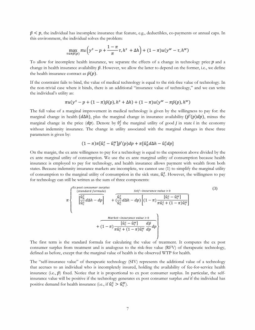
�̅�𝑝 < 𝑝𝑝, the individual has incomplete insurance that feature, e.g., deductibles, co-payments or annual caps. In this environment, the individual solves the problem:

max𝜏𝜏≤𝜋𝜋�̅�𝑝(𝑝𝑝)

𝜋𝜋𝑢𝑢 �𝑦𝑦𝑠𝑠 − 𝑝𝑝 +1 − 𝜋𝜋𝜋𝜋

𝜏𝜏,ℎ𝑠𝑠 + Δℎ� + (1 − 𝜋𝜋)𝑢𝑢(𝑦𝑦𝑤𝑤 − 𝜏𝜏,ℎ𝑤𝑤)

To allow for incomplete health insurance, we separate the effects of a change in technology price 𝑝𝑝 and a change in health insurance availability �̅�𝑝. However, we allow the latter to depend on the former, i.e., we define the health insurance contract as �̅�𝑝(𝑝𝑝).

If the constraint fails to bind, the value of medical technology is equal to the risk-free value of technology. In the non-trivial case where it binds, there is an additional “insurance value of technology,” and we can write the individual’s utility as:

𝜋𝜋𝑢𝑢(𝑦𝑦𝑠𝑠 − 𝑝𝑝 + (1 − 𝜋𝜋)�̅�𝑝(𝑝𝑝),ℎ𝑠𝑠 + Δℎ) + (1 − 𝜋𝜋)𝑢𝑢(𝑦𝑦𝑤𝑤 − 𝜋𝜋�̅�𝑝(𝑝𝑝),ℎ𝑤𝑤)

The full value of a marginal improvement in medical technology is given by the willingness to pay for: the marginal change in health (𝑑𝑑Δℎ), plus the marginal change in insurance availability (�̅�𝑝′(𝑝𝑝)𝑑𝑑𝑝𝑝), minus the marginal change in the price (𝑑𝑑𝑝𝑝). Denote by 𝑣𝑣�𝑗𝑗𝑖𝑖 the marginal utility of good 𝑗𝑗 in state 𝑖𝑖 in the economy without indemnity insurance. The change in utility associated with the marginal changes in these three parameters is given by:

(1 − 𝜋𝜋)𝜋𝜋[𝑢𝑢�𝑐𝑐𝑠𝑠 − 𝑢𝑢�𝑐𝑐𝑤𝑤]�̅�𝑝′(𝑝𝑝)𝑑𝑑𝑝𝑝 + 𝜋𝜋[𝑢𝑢�ℎ𝑠𝑠𝑑𝑑Δℎ − 𝑢𝑢�𝑐𝑐𝑠𝑠𝑑𝑑𝑝𝑝]

On the margin, the ex ante willingness to pay for a technology is equal to the expression above divided by the ex ante marginal utility of consumption. We use the ex ante marginal utility of consumption because health insurance is employed to pay for technology, and health insurance allows payment with wealth from both states. Because indemnity insurance markets are incomplete, we cannot use (1) to simplify the marginal utility of consumption to the marginal utility of consumption in the sick state, 𝑢𝑢�𝑐𝑐𝑠𝑠. However, the willingness to pay for technology can still be written as the sum of three components:

𝜋𝜋

⎩⎪⎨

⎪⎧

�𝑢𝑢�ℎ𝑠𝑠

𝑢𝑢�𝑐𝑐𝑠𝑠𝑑𝑑Δℎ − 𝑑𝑑𝑝𝑝�

���������

𝐸𝐸𝐸𝐸 𝑝𝑝𝑝𝑝𝑠𝑠𝑝𝑝 𝑐𝑐𝑝𝑝𝑐𝑐𝑠𝑠𝑐𝑐𝑐𝑐𝑐𝑐𝑐𝑐 𝑠𝑠𝑐𝑐𝑐𝑐𝑝𝑝𝑠𝑠𝑐𝑐𝑠𝑠 (𝑠𝑠𝑝𝑝𝑠𝑠𝑐𝑐𝑠𝑠𝑠𝑠𝑐𝑐𝑠𝑠 𝑓𝑓𝑝𝑝𝑐𝑐𝑐𝑐𝑐𝑐𝑠𝑠𝑠𝑠)

+ (𝑢𝑢�ℎ𝑠𝑠

𝑢𝑢�𝑐𝑐𝑠𝑠𝑑𝑑Δℎ − 𝑑𝑑𝑝𝑝) �(1 − 𝜋𝜋)

[𝑢𝑢�𝑐𝑐𝑠𝑠 − 𝑢𝑢�𝑐𝑐𝑤𝑤]𝜋𝜋𝑢𝑢�𝑐𝑐𝑠𝑠 + (1 − 𝜋𝜋)𝑢𝑢�𝑐𝑐𝑤𝑤

������������������������������

𝑆𝑆𝑐𝑐𝑠𝑠𝑓𝑓−𝑖𝑖𝑐𝑐𝑠𝑠𝑐𝑐𝑐𝑐𝑠𝑠𝑐𝑐𝑐𝑐𝑐𝑐 𝑣𝑣𝑠𝑠𝑠𝑠𝑐𝑐𝑐𝑐 > 0

+ (1 − 𝜋𝜋)[𝑢𝑢�𝑐𝑐𝑠𝑠 − 𝑢𝑢�𝑐𝑐𝑤𝑤]

𝜋𝜋𝑢𝑢�𝑐𝑐𝑠𝑠 + (1 − 𝜋𝜋)𝑢𝑢�𝑐𝑐𝑤𝑤 𝑑𝑑�̅�𝑝𝑑𝑑𝑝𝑝

𝑑𝑑𝑝𝑝���������������������

𝑀𝑀𝑠𝑠𝑐𝑐𝑀𝑀𝑐𝑐𝑝𝑝−𝑖𝑖𝑐𝑐𝑠𝑠𝑐𝑐𝑐𝑐𝑠𝑠𝑐𝑐𝑐𝑐𝑐𝑐 𝑣𝑣𝑠𝑠𝑠𝑠𝑐𝑐𝑐𝑐 > 0

⎭⎪⎬

⎪⎫

(3)

The first term is the standard formula for calculating the value of treatment. It computes the ex post consumer surplus from treatment and is analogous to the risk-free value (RFV) of therapeutic technology, defined as before, except that the marginal value of health is the observed WTP for health.

The “self-insurance value” of therapeutic technology (SIV) represents the additional value of a technology that accrues to an individual who is incompletely insured, holding the availability of fee-for-service health insurance (i.e., �̅�𝑝) fixed. Notice that it is proportional to ex post consumer surplus. In particular, the self-insurance value will be positive if the technology generates ex post consumer surplus and if the individual has positive demand for health insurance (i.e., if 𝑢𝑢�𝑐𝑐𝑠𝑠 > 𝑢𝑢�𝑐𝑐𝑤𝑤).

7

Finally, the “market-insurance value” (MIV) represents the incremental value of being able to use health insurance to substitute for the indemnity insurance market. Medical technology is essential to this substitution because health insurance can only be used to fund consumption of medical care. Mathematically, the market insurance value is the willingness to pay for a marginal increase in �̅�𝑝, the constraint on the level of fee-for-service health insurance. This will be positive as long as the individual is incompletely insured (i.e., if 𝑢𝑢�𝑐𝑐𝑠𝑠 >𝑢𝑢�𝑐𝑐𝑤𝑤). Another way to put it is that market-insurance value is the value of reducing the gap in the marginal utility of consumption across states, holding fixed the level of health.

The effect of ℎ𝑠𝑠 on the expression for value is of particular interest, because low values of ℎ𝑠𝑠 reflect diseases with high “unmet need” and vice-versa. For purposes of this argument, we will make the empirically realistic assumption that the marginal ex post willingness to pay for health improvement is falling in the baseline level of health, i.e., people who are sicker have higher willingness to pay for a given health improvement, and vice-versa.11 This assumption is supported by survey evidence suggesting that people value a given level of health investment more highly when provided to sicker patients (Nord, Richardson et al. 1995, Green and Gerard 2009, Linley and Hughes 2013). If this assumption obtains, two results follow. First, the full value of a medical technology is higher for diseases with a higher degree of unmet need, defined by lower values of ℎ𝑠𝑠. Second, the difference between the conventional value – i.e., ex post consumer surplus – and the full value grows as the degree of unmet need rises. This suggests that errors in the use of the standard approach are most likely for severe diseases with a poor current standard of care.

All the arguments above are derived on the margin, but the appendix shows how these arguments can be generalized to inframarginal improvements in treatment. Our aim here is to show that standard estimates of the value of technology that employ the willingness to pay for health will tend to underestimate the full value because they ignore the insurance value due to technology.

Finally, note also that expression (3) is unchanged if we allow for endogenous investments in prevention . Consider, for example, a new therapeutic treatment for an infectious disease, which can be prevented by avoiding infected individuals. Assuming that prevention is chosen optimally, the envelope theorem implies that the choice of prevention level will have no impact on the expression for the value of new treatment on the margin.

III: EMPIRICAL ESTIMATES OF THE VALUE OF THRAPEUTIC TECHNOLOGY We now present results from some simple calibration exercises that demonstrate that total insurance value of medical innovation is an empirically important concept. We first describe our estimation framework and explain how we parameterize our empirical model. We then conduct two different calibration exercises. The first employs data from a nationally representative set of individuals to estimate the risk-free and self-insurance values that follow from increases in the quality of life. The second exercise employs data from the Cost-Effectiveness Analysis Registry to generate estimates of the risk-free, self-insurance, and market-insurance values for a large set of real-world therapeutic innovations.

A: Estimation framework Generating quantitative estimates of the value of medical innovation requires specifying a functional form for utility. Following the existing literature on how health affects preferences for investment risk (Picone, Uribe

11 It is straightforward to show that this is equivalent to assuming 𝑣𝑣�𝑐𝑐𝑠𝑠𝑣𝑣�ℎℎ

𝑠𝑠 − 𝑣𝑣�ℎ𝑠𝑠𝑣𝑣�𝑐𝑐ℎ

𝑠𝑠 < 0. This condition necessarily holds for certain classes of utility functions, including the Cobb-Douglas specification.

8

et al. 1998, Edwards 2008), we assume that consumers have Cobb-Douglas period utility over consumption and health:

𝑢𝑢(𝑐𝑐,ℎ) =(𝑐𝑐𝛾𝛾ℎ1−𝛾𝛾)1−𝜎𝜎 − 1

1 − 𝜎𝜎 if 𝜎𝜎 ≠ 1

𝑢𝑢(𝑐𝑐,ℎ) = ln(𝑐𝑐𝛾𝛾ℎ1−𝛾𝛾) if 𝜎𝜎 = 1

where 𝛾𝛾 ∈ (0,1) affects the marginal rate of substitution between consumption and health and 𝜎𝜎 ≥ 0 affects the curvature of the utility function. The parameter 𝛾𝛾 drives the risk-free value of technology while the parameter 𝜎𝜎 drives risk aversion. This utility specification is convenient because it separates risk-aversion from the risk-free value placed on improvements in health.12 This allows us to hold the risk-free value of technology constant when estimating the effect of risk aversion on insurance values.

The parameter 𝜎𝜎 also determines the effect of a decrease in health on the marginal utility of consumption. The effect is negative if 𝜎𝜎 < 1 (negative state dependence) and positive if 𝜎𝜎 > 1 (positive state dependence). If 𝜎𝜎 = 1 then the marginal utility of consumption is independent of health (state-independent utility). All else equal, the value of transferring resources from the well state to the sick state is increasing in 𝜎𝜎.

We are only aware of one study that estimates the parameter 𝛾𝛾. Edwards (2008) examines the effect of health risk on investment decisions and concludes that a range of 0.155 to 0.443 for 𝛾𝛾 best fits the data. We therefore set 𝛾𝛾 = 0.3 in our analysis. Although employing alternative values of 𝛾𝛾 that are significantly higher or lower than 0.3 affects the levels of our estimates, it does not substantively change our conclusions concerning the ratio of the insurance value of technology to the risk-free value.13

Because there is little agreement regarding the sign, let alone the magnitude, of the state dependence of the utility function, we calibrate the parameter 𝜎𝜎 using estimates from studies of risk aversion.14 The Arrow-Pratt measure of relative risk aversion over consumption in our Cobb-Douglas utility specification is equal to 𝑅𝑅𝑐𝑐 =1 − 𝛾𝛾(1 − 𝜎𝜎) > 0 (Dardanoni 1988). The proper value of risk aversion among real-world populations remains controversial. Chetty (2006) estimates a risk aversion value of 0.15 to 1.78, but many studies have estimated much larger values.15 We adopt 𝜎𝜎 = 3 as our preferred estimate, which corresponds to 𝑅𝑅𝑐𝑐 = 1.6, but we also report results across a broad range of risk assumptions. As we shall see, the values of SIV and MIV relative to RFV depend greatly on the assumed value of 𝜎𝜎.

12 We also considered a multiplicative utility model such as that in Murphy and Topel (2006): 𝑢𝑢(𝑐𝑐, ℎ) = ℎ𝑢𝑢(𝑐𝑐). The advantage of a multiplicative utility is that it allows one to separate the impact of risk aversion from the impact of state dependence. The disadvantage, however, is that changes in risk aversion 𝜎𝜎 impact not only the insurance value of innovation but also the risk-free value of technology. Because we think the later a more important feature, we focus on the Cobb-Douglas model. We will conduct a calibration exercise with multiplicative utility and report it in a future draft in order to check the robustness of our empirical analysis and make it more comparable to Murphy and Topel.

13 Setting 𝛾𝛾 = 0.15 results in insurance values that are more than double the RFV, while setting 𝛾𝛾 = 0.6 results in insurance values that are one-half the size of RFV.

14 Finkelstein et al. (2013), Sloan et al (1988), and Viscusi and Evans (1990) find evidence of negative state dependence. Edwards (2008) and Lillard and Weiss (1988) find evidence of positive state dependence. Evans and Viscusi (1991) find no evidence of state dependence.

15 A less than comprehensive list includes Barsky et al. (1997), Cohen and Einav (2005), Kocherlakota (1996), and Mehra and Prescott (1985).

9

Unless otherwise noted, we assume throughout that income in both the sick and well states, 𝑦𝑦𝑠𝑠 and 𝑦𝑦𝑤𝑤, is equal to $120,000, which is approximately the value of full income (consumption plus value of leisure) for a typical individual. This assumption is conservative because it minimizes the value of transferring wealth from the healthy state to the sick state and does not incorporate the documented empirical finding that poor health tends to decrease income (Smith 1999). Employing an alternative, lower value for 𝑦𝑦𝑠𝑠 would increase our estimates of both the self-insurance and market-insurance values of technology.

Our calibration exercises require us to quantify health in some manner. We accomplish this by employing quality of life measures from our data sets, described below. Because health has no natural units, all measures are normalized without loss of generality so that they range from 0 to 1. These endpoints can be thought of as representing “death” and “perfect health”, respectively. The subjective nature of the data and the multidimensional nature of health mean these measures are necessarily imperfect. Nevertheless, we build on established literatures of health measurement in order to lend our measurement strategy a firmer foundation.

Because some medical technologies may generate large increases in health, we employ the inframarginal analogue to our theoretical model in order to produce accurate estimates of risk free value (RFV), self-insurance value (SIV), and market-insurance value (MIV). We provide those formulas in our appendix. Finally, we report all estimates of RFV, SIV, and MIV from an ex ante perspective. Thus, our estimates should be regarded as the values accruing to an individual who is facing a risk of illness rather than to an individual who is already ill.

Before we turn to our empirical estimates, we illustrate how RFV, SIV, and MIV change as a function of a technology’s price, given our parameter assumptions. Figure 1 displays the results for the case where ℎ𝑠𝑠 =0.8 and ∆ℎ = 0.2. When the price of treatment is low, most of its value comes from RFV and SIV. As the price increases, the value of transferring money across states becomes more important, as reflected by the increasing value of MIV.16 The risk-free and total values are decreasing in price, as expected.

B: Aggregate value of gains to quality of life There is substantial evidence that the average quality of life has improved dramatically over the past fifty years. The proportion of elderly who are disabled has decreased, and the proportion who are active has increased (Cutler 2005). Previous work by Murphy and Topel (2006) has estimated that the increase in quality of life is actually more valuable than the accompanying increase in life expectancy. Our first calibration exercise aims to understand how this value changes when one accounts for the insurance value of innovation when indemnity insurance markets are incomplete and consumers only have access to health insurance.

We accomplish this by estimating the lifetime benefits of an increase in quality of life, ∆ℎ, comparable to that considered in Murphy and Topel (2006) using data from a nationally representative sample of individuals from MEPS. We do not account for the cost of technology, i.e., we assume the price of technology is zero, which means our simulated increase in quality of life will generate self-insurance value, but no market insurance value. Including cost would lower the estimate of SIV but this would be at least partially offset by an increase in MIV.

The theoretical model presented in the first half of this paper allowed for only one possible sick state. In this section we generalize the model to allow for a continuum of possible states. Let the probability density function associated with these health states be 𝑓𝑓(ℎ𝑠𝑠). Then

16 RFV always decreases with price and MIV always increases with price. SIV depends on consumer surplus (which decreases in price) and the difference in marginal utilities across states, which increases in price. Thus, the overall effect of price on SIV cannot be signed in general because it depends on the relative values of consumer surplus and the difference in marginal utilities.

10

𝑅𝑅𝑅𝑅𝑅𝑅 = � 𝐺𝐺𝑅𝑅(𝑦𝑦,𝑓𝑓(ℎ𝑠𝑠), ℎ𝑤𝑤,ℎ𝑠𝑠,Δ(ℎ𝑠𝑠)) 𝑓𝑓(ℎ𝑠𝑠)𝑑𝑑ℎ𝑠𝑠1

0

𝑆𝑆𝑆𝑆𝑅𝑅 = � 𝐺𝐺𝑆𝑆(𝑦𝑦,𝑓𝑓(ℎ𝑠𝑠),ℎ𝑤𝑤 ,ℎ𝑠𝑠,Δ(ℎ𝑠𝑠)) 𝑓𝑓(ℎ𝑠𝑠)𝑑𝑑ℎ𝑠𝑠1

0

where the functions 𝐺𝐺𝑅𝑅(𝑦𝑦,𝑓𝑓(ℎ𝑠𝑠), ℎ𝑤𝑤,ℎ𝑠𝑠,Δ(ℎ𝑠𝑠)) and 𝐺𝐺𝑆𝑆(𝑦𝑦,𝑓𝑓(ℎ𝑠𝑠),ℎ𝑤𝑤 ,ℎ𝑠𝑠,Δ(ℎ𝑠𝑠)) are the inframarginal analogues to the marginal RFV and SIV expressions equations (2) and (3) after they have been modified to account for multiple health states. (The multiple-state modifications and the inframarginal analogues are defined in the sections B and C, respectively, of the appendix.) We allow the value of the ex post health improvement, Δ(ℎ𝑠𝑠), to depend on the health state. The total amount of health risk that individuals face depends on the distribution of possible health states, 𝑓𝑓(ℎ𝑠𝑠).

We construct an empirical estimate of the probability density function, 𝑓𝑓(ℎ𝑠𝑠), from nationally representative data on self-reported health status obtained from the 2000-2003 Medical Expenditure Panel Surveys. These surveys include five questions regarding the extent of the respondent’s problems in mobility, self-care, daily activities, pain, and anxiety/depression. They also include an additional variable that combines the responses to these questions into a quality of life index that ranges from 0 to 1.17 We use that index to construct an empirical estimate of the probability density function, 𝑓𝑓(ℎ𝑠𝑠).

In order to construct 𝑓𝑓(ℎ𝑠𝑠), we first estimate health state deciles by age group and gender for each survey. We then average those estimates across the four surveys. Our results are reported in Table 1. It shows that the 10th percentile of health status for 18-34 year-old males is equal to 0.726. For each decile, health status declines with age, as expected. Conditional on age, males are estimated to have a higher quality of life than females. In every group, the healthiest decile enjoys perfect health.

Next, we estimate how much a consumer facing the health risk distribution described in Table 1 would be willing to pay, ex ante, for a hypothetical increase in the quality of life in each possible realized state. We assume that ℎ𝑤𝑤 = 1 and set the hypothetical increase equal to Δ(ℎ𝑠𝑠) = min (ℎ𝑠𝑠 + 0.1,1) . This health increase is in line with the hypothetical increase considered by Murphy and Topel (2006).18

Our results are displayed in Table 2. They show that the total annual value of the health increase is equal to $13,647 for males between the ages of 18 and 34. This total can be broken down into $11,027 of risk-free value and $2,620 of self-insurance value. Both RFV and SIV are increasing with age because the elderly are less healthy and thus have more to gain from health improvements. Young individuals, by contrast, already have a high probability of enjoying perfect health, which cannot be improved.

RFV is responsible for the bulk of the health gain when individuals are young, but the fraction of the gain due to SIV increases steadily with age and actually exceeds the fraction due to RFV for the oldest age group. This is due to the large dispersion in health states for the elderly, as shown in Table 1. Because the elderly face the most health risk, they enjoy the highest insurance gains from an increase in the quality of life.

17 About 2% of the sample has a negative value for the index, indicating a health status worse than death. We recode them to have a value equal to 0.01. This has no effect on our results.

18 Murphy and Topel (2006) assume that advances in quality of life are related to the declines in mortality from 1970-2000. Life expectancy increased by 8.7 percent during that period. Our hypothetical quality of life increase, when averaged across gender, age, and health states, increases the average index by 7.7 percent.

11

Finally, we generate an estimate of the per capita life-time value of these health gains for an 18-year-old by aggregating over age groups. We discount estimates by the probability of survival and by a rate of interest equal to four percent.19 Those results, displayed in Table 3, show that the hypothetical health increase we consider generates about $550,000 and $720,000 in risk-free value for an 18-year-old male and female, respectively. This is in line with the range of $400,000 to $600,000 estimated by Murphy and Topel (2006) for 30-year-olds. (They do not estimate values for earlier ages.) We also estimate that the self-insurance value adds fifty percent to the risk-free value for males and seventy percent for females. This suggests that the value of advances in the quality of life may be significantly higher than has previously been recognized.

C: Estimates of the insurance value of therapeutic innovations In our second calibration exercise, we estimate the risk-free, self-insurance, and market-insurance values for real-world therapeutic technologies. Our theoretical model is static. In the real-world, diseases and treatments evolve over a period of time. However, since our data (described below) do not contain information on how each technology produces health improvements over time, the static setup sacrifices little generality. In keeping with these data limitations, we assume that the health benefits and costs are constant over time. Thus, quantifying the annualized value of a technology is essentially equivalent to quantifying the long-term value.

In order to calibrate the components of value for a particular technology, we need data on four parameters: the annual price of the technology (𝑝𝑝), the baseline health level prior to treatment (ℎ𝑠𝑠), the perfectly well health level (ℎ𝑤𝑤), and the annualized health improvement produced by the technology (𝛥𝛥ℎ). In our exercise, we set ℎ𝑤𝑤 = 1. We obtain the remaining data from the Cost-Effectiveness Analysis Registry (CEAR). CEAR is a collection of several thousand cost-effectiveness studies published between 1976 and 2012.20 A study is included in the database if it (1) contains original research; (2) measures health benefits in uniform units called Quality-Adjusted Life Years (QALYs); and (3) is published in English.

A QALY ranges from 0 to 1. It incorporates changes in both morbidity and mortality, and converts them into an “equivalent” (in terms of what consumers will accept) number of “years of good health.” For example, if individuals are indifferent between living 9 months in perfect health and living 12 months on dialysis, then one year of life on dialysis is considered equal to 9/12 = 0.75 “quality-adjusted” years. QALYs thus provide a convenient, standardized metric for comparing health benefits across different treatments.21

Our theoretical model pertains to changes in current period health, or morbidity. One shortcoming of the CEAR data is that its measure of health improvement does not distinguish between longevity improvements and morbidity improvements. Attributing the improvement entirely to a decrease in morbidity will thus cause upward bias in our estimation. However, we are primarily interested in estimating the value of self-insurance relative to market-insurance. Our results are substantively unchanged if we conservatively assume that only one-half of the health improvement is due to a decrease in morbidity. Moreover, our results throughout can

19 Survival probabilities are obtained from www.mortality.org. Discount rates are calculated for the midpoint of the age group. For example, the expected risk-free value for an 18-year-old male for the period covering ages 18-34 is equal to $11,027 × 17 × 0.99886/(1 + 0.04)17/2 , where the first term comes from Table 1, 17 = 34 − 18 + 1, the third term is the probability of surviving from age 18 to age 35, and the last term is the discount rate.

20 See research.tufts-nemc.org/cear4/AboutUs/WhatistheCEARegistry.aspx for more information.

21 Employing QALY’s imposes restrictions on the risk structure of the utility function when operating in an environment that allows for changes in both longevity and morbidity Bleichrodt, H. and J. Quiggin (1999). "Life-cycle preferences over consumption and health: when is cost-effectiveness analysis equivalent to cost-benefit analysis?" J Health Econ 18(6): 681-708.. However, we are only estimating the value of changes in morbidity, which allows for a more general specification of the utility function Hammitt, J. K. (2013). "Admissible Utility Functions for Health, Longevity, and Wealth: Integrating Monetary and Life-Year Measures." Journal of Risk and Uncertainty 47: 311-325..

12

still be interpreted as demonstrating how insurance value evolves as current period health varies, since the precise identity of the medical technologies in the CEAR database is not central to our key conclusions.

The annualized price of treatment (𝑝𝑝), health improvements (∆ℎ), and the health baseline (ℎ𝑠𝑠) are easily recovered from cost-effectiveness data. For example, a typical study computes costs and benefits over a horizon of 𝑇𝑇 periods as:

𝐶𝐶𝐶𝐶𝑠𝑠𝐶𝐶 = 𝑃𝑃𝑃𝑃𝑖𝑖𝑐𝑐𝑃𝑃 = �𝑝𝑝𝑝𝑝�1− 𝑃𝑃𝑝𝑝�𝑝𝑝

𝑇𝑇−1

𝑝𝑝=0

𝐵𝐵𝑃𝑃𝐵𝐵𝑃𝑃𝑓𝑓𝑖𝑖𝐶𝐶 = �∆ℎ𝑝𝑝(1− 𝑃𝑃ℎ)𝑝𝑝𝑇𝑇−1

𝑝𝑝=0

The total cost of an intervention depends on the annual incremental cost, 𝑝𝑝𝑝𝑝, and is discounted at the rate 𝑃𝑃𝑝𝑝 over a time horizon of 𝑇𝑇 years. The total benefit is measured in annual incremental QALYs, ∆ℎ𝑝𝑝 , and is discounted at the rate 𝑃𝑃ℎ.22 The cost-effectiveness ratio is equal to 𝐶𝐶𝐶𝐶𝑠𝑠𝐶𝐶/𝐵𝐵𝑃𝑃𝐵𝐵𝑃𝑃𝑓𝑓𝑖𝑖𝐶𝐶.

The majority of cost-effectiveness studies do not specify an entire time path for {𝑝𝑝𝑝𝑝 ,𝛥𝛥ℎ𝑝𝑝}. This is consistent with our assumption of a constant flow every period, characterized by {𝑝𝑝,𝛥𝛥ℎ}. These constant flow values are easily derived from the equations above, given information on total cost, total benefit, discount rates, and time horizon, imposing the constraints that 𝑝𝑝𝑝𝑝 = 𝑝𝑝 and 𝛥𝛥ℎ𝑝𝑝 = 𝛥𝛥ℎ. Given the assumption of constant utility flow, it is without loss of generality that we consider the annualized cost and health benefit of medical technologies. Thus, 𝛥𝛥ℎ reflects the annual improvement in health enjoyed by a patient, and 𝑝𝑝 reflects the annual price paid for the associated technology.

CEAR reports estimates of cost-effectiveness ratios (𝐶𝐶𝐶𝐶𝑠𝑠𝐶𝐶/𝐵𝐵𝑃𝑃𝐵𝐵𝑃𝑃𝑓𝑓𝑖𝑖𝐶𝐶) for a wide variety of diseases and treatments. We exclude studies that do not report estimates of 𝐶𝐶𝐶𝐶𝑠𝑠𝐶𝐶 and 𝐵𝐵𝑃𝑃𝐵𝐵𝑃𝑃𝑓𝑓𝑖𝑖𝐶𝐶 separately and that do not report time horizon or discount rates. CEAR classifies each study into different intervention types. We confine our attention to treatments, rather than preventive technologies (e.g., vaccines), and thus include any CEAR study classified “pharmaceutical”, “surgical”, “medical device”, or “medical procedure”. 23 CEAR provides information on the total cost, total benefit, discount rates, and time horizon for each study.24 As mentioned above, these data elements are sufficient to estimate the annual flow terms, {𝑝𝑝,𝛥𝛥ℎ}.

CEAR also reports the “health state utility weights” for each of the health states considered by a particular cost-effectiveness study. These cardinal measures range from 0 to 1 and are used to proxy for ℎ𝑠𝑠, the quality of life in the pre-treatment (sick) state. For example, suppose there are two health states, A and B, representing patients at different levels of illness severity. These two states correspond to the utility weights 𝑤𝑤𝑠𝑠 and 𝑤𝑤𝑏𝑏. If, prior to treatment, half of the patients are in health state A and the other half are in B, then ℎ𝑠𝑠 = (𝑤𝑤𝑠𝑠 + 𝑤𝑤𝑏𝑏)/2. Since CEAR does not report what fraction of the patients is in each health state for

22 The discount rates 𝑃𝑃𝑝𝑝 and 𝑃𝑃ℎ are usually equal to each other. Only 8% of the studies in CEAR discount costs and benefits using different rates.

23 We exclude the categories “care delivery”, “diagnostic”, “health education or behavior”, “immunization”, “none/na”, “other”, and “screening” because these types of technologies are more likely to be preventative rather than therapeutic. See the appendix for a discussion of how to estimate the value of preventative care.

24 Some studies report a time horizon of “lifetime” rather than a specific number of years. In those cases we assume a horizon of 85 years.

13

either the pre- or post-treatment groups, we assume that pre-treatment patients are uniformly distributed across health states.

CEAR assigns each treatment to one of seventy different disease categories. We match each category to nationally representative estimates of annual disease incidence obtained from the Medical Expenditure Panel Survey. See the data appendix for details.

Our final sample of therapeutic medical technologies consists of 1,797 observations. Summary statistics are provided in Table 4. Figure 2 displays the distribution of ∆ℎ, in units of annual QALYS gained, in our sample of therapeutic innovations. The majority of treatments produce small, annualized improvements in health (∆ℎ < 0.05), but a few treatments produce large improvements, which skews the sample to the right. For example, dialysis treatment for end-stage renal disease increases the annual quality of life by ∆ℎ = 0.33 QALYs.

Figure 3 displays the distribution of treatment prices in this sample. The sample is again skewed to the right, with the vast majority of treatments costing less than $5,000. Three very expensive treatments top the list with prices of approximately $150,000 per year: left ventricular assist devices for heart-failure patients and two different inhibitors for treatment of hemophilia. Although expensive, each of these three treatments generates large annual health improvements (∆ℎ ≈ 0.15) . Not all expensive treatments are valuable, however: interferon beta-1b, a treatment for multiple sclerosis that helps prevent patients from becoming wheelchair-dependent, costs $22,000 per year but generates little annual health improvement (∆ℎ = 0.009) (Forbes, Lees et al. 1999).

We now turn to the estimates from our model. Figure 4 shows that the distribution of RFV in our sample is concentrated near zero and skewed to the right. This indicates that outliers will have a significant influence on mean values, and that analysis by quantiles may provide useful additional information to analysis of means. Figure 4 also shows that there are several technologies that generate negative RFV, i.e., the ex post costs of these technologies exceeds the ex post benefits.

We report the mean and the 10th, 50th, and 90th percentiles of our estimates in Table 5 for values of 𝜎𝜎 ranging from 0.5 to 8, which corresponds to a relative risk aversion range of 0.85 to 3.1. The mean value of RFV, which is not a function of the parameter 𝜎𝜎, is $1,335. The means of SIV and MIV for our preferred specification, 𝜎𝜎 = 3, are $1,796 and $83, respectively. The gains from SIV and MIV are increasing in 𝜎𝜎 because that parameter is linked to risk aversion, which boosts insurance value. The means of our estimates are substantially larger than the medians due to the skewness of the distribution (see Figure 4).

When 𝜎𝜎 is less than 1, consumers exhibit negative state dependence and will not demand insurance in the sick state unless the price of treatment is sufficiently large. This is reflected in the negative values of MIV in the first row of Table 5. When 𝜎𝜎 is greater than or equal to 1, MIV will be positive for any treatment with a positive price.

Table 6 normalizes the SIV and MIV estimates in Table 5 by their corresponding RFV values. When evaluated at the mean for 𝜎𝜎 = 3, it shows that each dollar of RFV generates $1.34 in SIV and $0.06 of MIV. In other words, properly accounting for the total insurance benefits of therapeutic innovation increases its value by 140%.

Our mean estimates of MIV are small because the prices of most of the treatments in our sample are low relative to annual income. The value of MIV increases substantially when the price of treatment is a significant fraction of an individual’s wealth, as Figure 5 vividly demonstrates. Table 7 shows how our estimates vary by price quantiles of treatment. RFV does not always increase with price, indicating that costly treatments do not necessarily confer correspondingly large health benefits on the consumer. When risk aversion becomes large, the estimated values for MIV approach and sometimes even exceed RFV. This agrees

14

with the notion that insurance is more valuable for expensive items than for cheap items, regardless of whether those items generate consumer surplus.

Our estimates can be employed to compare consumers’ willingness to pay for the self-insurance value of technology to their willingness to pay for the insurance value of health insurance. One complication is that, whereas SIV is entirely due to technology, MIV is attributable to both technology and health insurance: its value is equal to zero without one or the other. According to Table 6, however, even if MIV is entirely credited to health insurance, technology creates over 20 times as much value as health insurance ($1.34 vs. $0.06 of value) when evaluated at the mean.

Treatments for diseases with high “unmet need”, defined in our framework as diseases with low values of ℎ𝑠𝑠, are of particular interest, because there is much controversy surrounding their reimbursement. Survey evidence indicates that people believe that, all else equal, it is more beneficial to treat patients whose baseline level of health is lower. Moreover, even health technology assessment authorities known for their strictness tend to agree with this view, and often make coverage exceptions for expensive drugs that treat conditions where the need for new treatments is extreme, e.g., orphan diseases with few options and terminal diseases like cancer (Lancet, 2010).

Figure 6 and Figure 7 illustrate how our estimate of the full value of treatment, and its three components, vary by health status. Treatments for diseases with high unmet are indeed valuable, but Figure 7 reveals that very little of that value is generated by RFV, the component corresponding to the traditional valuation of medical technology. Figure 8 demonstrates this same point by showing that RFV significantly undervalues treatments with high unmet need. This suggests that – in line with public opinion – the standard approach to valuation is most inappropriate in cases where patients are extremely sick.

Finally, we note that the estimates presented so far are conservative because we have assumed that the parameters governing income in the sick and well states are both equal to $120,000. If income in the sick state is lower, as is often the case for debilitating diseases like multiple sclerosis or Parkinson’s disease, then the relative values of SIV and MIV will increase because the value of being able to transfer resources from the well to the sick state increases. Table 8 shows how our estimates change if we assume that income in the sick state, 𝑦𝑦𝑠𝑠, is equal to $60,000 instead of $120,000. Under this scenario, instead of being roughly the same size as RFV, our estimates of SIV plus MIV for our preferred specification (𝜎𝜎 = 3) are about four times as large as our estimate of RFV.

IV: CONCLUSION When real-world health insurance markets are imperfect, risk-averse consumers derive value from medical technologies that limit the consequences of bad events and thereby expand the reach of financial health insurance. We refer to these values as the self-insurance, and market-insurance values of medical technology.

These theoretical observations are empirically meaningful. New medical technologies treating disease provide substantial insurance value above and beyond standard consumer surplus. Under plausible assumptions, the insurance value substantially exceeds the risk-free value. Notably, self-insurance value of therapeutic technology is often a much larger contributor of insurance value than market insurance value from health insurance. The latter point suggests that medical technology alone does more to reduce health risk than financial health insurance.

Our argument also suggests that the academic literature, which tends to focus exclusively on the standard consumer surplus value of medical technology, may have failed to capture a major part of its value. For example, Murphy and Topel (2006) value health increases over the past century at over $1 million per person. Our results suggest that accounting for uncertainty could significantly increase their estimates.

15

The ability of medical innovation to function as an insurance device influences not just the level of value, but also the relative value of alternative medical technologies. The conventional value framework overstates the value of technologies that treat mild disease, and penalizes those that treat the most severe illnesses. This helps explain why health technology access decisions driven by cost-effectiveness considerations alone often seem at odds with public opinion. For example, survey evidence suggests that representative respondents evaluating equally “cost-effective” technologies strictly prefer paying for the one that treats the most severe illness (Nord, Richardson et al. 1995).

From a normative point of view, our analysis also implies that the rate of innovation functions in a manner similar to policies or market forces that complete or improve the efficiency of insurance markets. Increases in the pace of medical innovation reduce overall physical risks to health, and thus function in a manner similar to expansions in health insurance. As a result, policymakers concerned about improving the management of health risks should view the pace of medical innovation as an important lever to influence and maintain. US policymakers have focused their efforts on improving health insurance access and design. While these are worthy goals, medical innovation policy may have an even greater impact on reducing risks from health.

More practically, our analysis informs the contemporary debate over how new medical technologies should be reimbursed. The United Kingdom provides an instructive example, as the UK health authorities hew closely to the use of ex post consumer surplus as a measure of value for a new technology, and thus a guide to how generously it should be reimbursed. Perhaps as a result, the UK performs poorly in the reimbursement of drugs to treat cancer, which has motivated legislators there to provide exceptional reimbursement for such products, above and beyond what the UK health authorities dictate (Lancet, 2010). Controversy has erupted over the appropriateness of this approach, and the legislation has drawn a great deal of criticism (Lancet, 2010). Yet, our analysis illuminates how the severe nature of cancer might contribute to the major misalignment between the standard economic approach to valuing medical technology and the preferences of legislators and voters. The policy lesson is that more attention needs to be paid by third-party payers and other health policymakers to covering treatments for diseases with high unmet needs. Exceptional treatments for terminal illness, orphan diseases, and diseases that remain poorly understood and treated are needed in order to align payment policies with the values of consumers. Moreover, the standard economic approach to valuing health technology should itself work towards alignment with the preferences of healthy consumers and sick patients.

16

REFERENCES (2010). "New 50 million cancer fund already intellectually bankrupt." Lancet 376(9739): 389. Altman, S. H. and R. Blendon (1977). "Medical Technology: The Culprit Behind Health Care Costs? Proceedings of the 1977 Sun Valley Forum on National Health." Barsky, R. B., F. T. Juster, M. S. Kimball and M. D. Shapiro (1997). "Preference parameters and behavioral heterogeneity: An experimental approach in the health and retirement study." The Quarterly Journal of Economics 112(2): 537-579. Bleichrodt, H. and J. Quiggin (1999). "Life-cycle preferences over consumption and health: when is cost-effectiveness analysis equivalent to cost-benefit analysis?" J Health Econ 18(6): 681-708. Chandra, A. and J. Skinner (2012). "Technology Growth and Expenditure Growth in Health Care." Journal of Economic Literature 50(3): 645-680. Chetty, R. (2006). "A new method of estimating risk aversion." American Economic Review 96(5): 1821-1834. Cohen, A. and L. Einav (2007). "Estimating Risk Preferences from Deductible Choice." American economic review 97(3): 745-788. Cutler, D. M. (2005). Your money or your life: strong medicine for America's health care system, Oxford University Press, USA. Dardanoni, V. (1988). "Optimal Choices Under Uncertainty: The Case of Two-Argument Utility Functions." The Economic Journal 98(391): 429-450. Edwards, R. D. (2008). "Health risk and portfolio choice." Journal of Business & Economic Statistics 26(4): 472-485. Ehrlich, I. and G. S. Becker (1972). "Market insurance, self-insurance, and self-protection." The Journal of Political Economy 80(4): 623-648. Forbes, R. B., A. Lees, N. Waugh and R. J. Swingler (1999). "Population based cost utility study of interferon beta-1b in secondary progressive multiple sclerosis." BMJ 319(7224): 1529-1533. Goddeeris, J. H. (1984). "Medical insurance, technological change, and welfare." Economic Inquiry 22(1): 56-67. Green, C. and K. Gerard (2009). "Exploring the social value of health-care interventions: a stated preference discrete choice experiment." Health Econ 18(8): 951-976. Hammitt, J. K. (2013). "Admissible Utility Functions for Health, Longevity, and Wealth: Integrating Monetary and Life-Year Measures." Journal of Risk and Uncertainty 47: 311-325. Kocherlakota, N. R. (1996). "The equity premium: It's still a puzzle." Journal of Economic Literature 34(1): 42-71. LaCronique, J. F. and S. Sandier (1981). "Technological innovation: cause or effect of increasing health expenditures." Innovation in Health Policy and Service Delivery: A Cross-National Perspective, Oelgeschlaher, Gunn and Hain, Cambridge, MA. Lakdawalla, D. and N. Sood (2009). "Innovation and the welfare effects of public drug insurance." Journal of public economics 93(3-4): 541-548. Linley, W. G. and D. A. Hughes (2013). "Societal views on NICE, Cancer Drugs Fund, and Value Based Pricing Criteria for Prioritising Medicines: A Cross-Sectionalk Survey of 4118 Adults in Great Britain." Health Economics 22(8): 948-964. Mehra, R. and E. C. Prescott (1985). The Equity Premium: A Puzzle. Journal of Monetary Economics. Murphy, K. M. and R. H. Topel (2006). "The Value of Health and Longevity." Journal of Political Economy 114(5). Murphy, K. M. and R. H. Topel (2006). "The Value of Health and Longevity." Journal of Political Economy 114(5): 871-904. Newhouse, J. P. (1992). "Medical Care Costs: How Much Welfare Loss?" The Journal of Economic Perspectives 6(3): 3-21. Nord, E., J. Richardson, A. Street, H. Kuhse and P. Singer (1995). "Maximizing health benefits vs egalitarianism: an Australian survey of health issues." Soc Sci Med 41(10): 1429-1437.

17

Okunade, A. A. and V. N. R. Murthy (2002). "Technology as a ‘major driver’ of health care costs: a cointegration analysis of the Newhouse conjecture." Journal of Health Economics 21(1): 147-159. Philipson, T. J. and A. B. Jena (2006). "Who benefits from new medical technologies? Estimates of consumer and producer surpluses for HIV/AIDS drugs." Forum for Health Economics & Policy 9(2). Picone, G., M. Uribe and R. Mark Wilson (1998). "The effect of uncertainty on the demand for medical care, health capital and wealth." Journal of Health Economics 17(2): 171-185. Pliskin, J. S., D. S. Shepard and C. W. Milton (1980). "Utility functions for life years and health status." Operations Research 28(1): 206-224. Showstack, J. A., M. H. Stone and S. A. Schroeder (1985). "The role of changing clinical practices in the rising costs of hospital care." New England Journal of Medicine 313(19): 1201-1207. Smith, J. P. (1999). "Healthy Bodies and Thick Wallets: The Dual Relation between Health and Economic Status." Journal of Economic Perspectives 13(2): 145-166. Viscusi, W. K. (1993). "The Value of Risks to Life and Health." Journal of Economic Literature 31(4): 1912-1946. Weisbrod, B. A. (1991). "The Health Care Quadrilemma: An Essay on Technological Change, Insurance, Quality of Care, and Cost Containment." Journal of Economic Literature 29(2): 523-552. Wilensky, G. (1990). "Technology as culprit and benefactor." The Quarterly review of economics and business 30(4): 45. Yin, W., J. R. Penrod, R. Maclean, D. N. Lakdawalla and T. Philipson (2012). "Value of survival gains in chronic myeloid leukemia." American Journal of Managed Care 18(11 Suppl): S257-264. Zweifel, P., S. Felder and M. Meiers (1999). "Ageing of population and health care expenditure: a red herring?" Health economics 8(6): 485-496.

APPENDIX

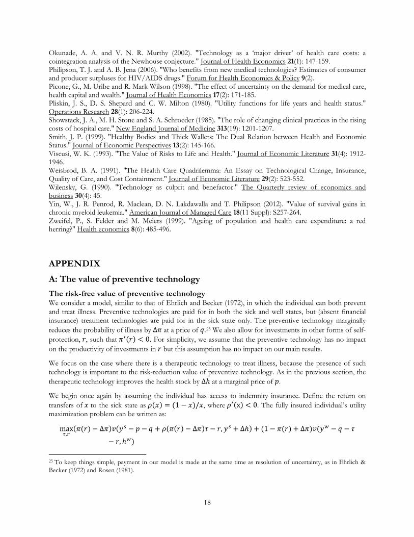
A: The value of preventive technology The risk-free value of preventive technology We consider a model, similar to that of Ehrlich and Becker (1972), in which the individual can both prevent and treat illness. Preventive technologies are paid for in both the sick and well states, but (absent financial insurance) treatment technologies are paid for in the sick state only. The preventive technology marginally reduces the probability of illness by Δ𝜋𝜋 at a price of 𝑞𝑞.25 We also allow for investments in other forms of self-protection, 𝑃𝑃, such that 𝜋𝜋′(𝑃𝑃) < 0. For simplicity, we assume that the preventive technology has no impact on the productivity of investments in 𝑃𝑃 but this assumption has no impact on our main results.

We focus on the case where there is a therapeutic technology to treat illness, because the presence of such technology is important to the risk-reduction value of preventive technology. As in the previous section, the therapeutic technology improves the health stock by Δℎ at a marginal price of 𝑝𝑝.

We begin once again by assuming the individual has access to indemnity insurance. Define the return on transfers of 𝑥𝑥 to the sick state as 𝜌𝜌(𝑥𝑥) = (1 − 𝑥𝑥)/𝑥𝑥, where 𝜌𝜌′(x) < 0. The fully insured individual’s utility maximization problem can be written as:

max𝜏𝜏,𝑐𝑐

(𝜋𝜋(𝑃𝑃) − Δ𝜋𝜋)𝑣𝑣(𝑦𝑦𝑠𝑠 − 𝑝𝑝 − 𝑞𝑞 + 𝜌𝜌(𝜋𝜋(𝑃𝑃) − Δ𝜋𝜋)𝜏𝜏 − 𝑃𝑃,𝑦𝑦𝑠𝑠 + Δℎ) + (1 − 𝜋𝜋(𝑃𝑃) + Δ𝜋𝜋)𝑣𝑣(𝑦𝑦𝑤𝑤 − 𝑞𝑞 − 𝜏𝜏

− 𝑃𝑃,ℎ𝑤𝑤)

25 To keep things simple, payment in our model is made at the same time as resolution of uncertainty, as in Ehrlich & Becker (1972) and Rosen (1981).

18

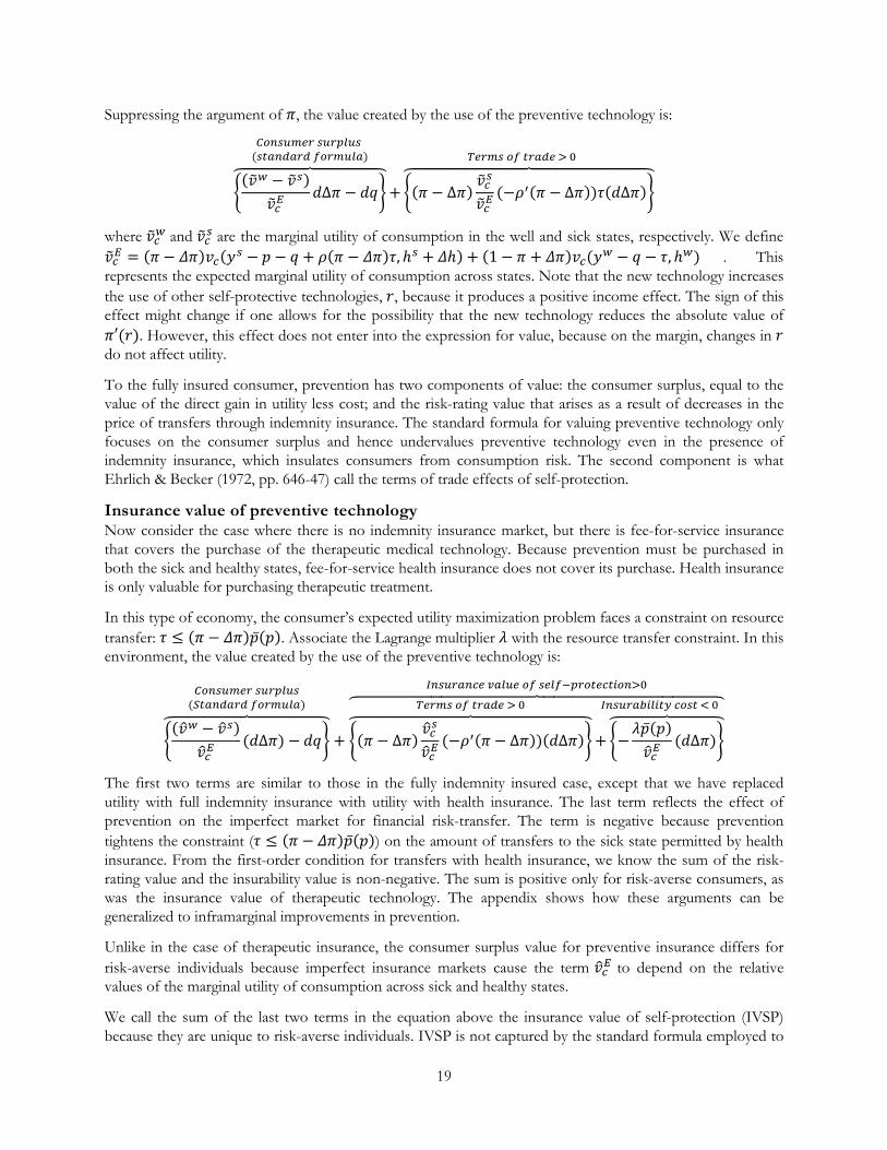
Suppressing the argument of 𝜋𝜋, the value created by the use of the preventive technology is:

�(𝑣𝑣�𝑤𝑤 − 𝑣𝑣�𝑠𝑠)

𝑣𝑣�𝑐𝑐𝐸𝐸𝑑𝑑Δ𝜋𝜋 − 𝑑𝑑𝑞𝑞�

���������������

𝐶𝐶𝑝𝑝𝑐𝑐𝑠𝑠𝑐𝑐𝑐𝑐𝑐𝑐𝑐𝑐 𝑠𝑠𝑐𝑐𝑐𝑐𝑝𝑝𝑠𝑠𝑐𝑐𝑠𝑠 (𝑠𝑠𝑝𝑝𝑠𝑠𝑐𝑐𝑠𝑠𝑠𝑠𝑐𝑐𝑠𝑠 𝑓𝑓𝑝𝑝𝑐𝑐𝑐𝑐𝑐𝑐𝑠𝑠𝑠𝑠)

+ �(𝜋𝜋 − Δ𝜋𝜋)𝑣𝑣�𝑐𝑐𝑠𝑠

𝑣𝑣�𝑐𝑐𝐸𝐸(−𝜌𝜌′(𝜋𝜋 − Δ𝜋𝜋))𝜏𝜏(𝑑𝑑Δ𝜋𝜋)�

�������������������������𝑇𝑇𝑐𝑐𝑐𝑐𝑐𝑐𝑠𝑠 𝑝𝑝𝑓𝑓 𝑝𝑝𝑐𝑐𝑠𝑠𝑠𝑠𝑐𝑐 > 0

where 𝑣𝑣�𝑐𝑐𝑤𝑤 and 𝑣𝑣�𝑐𝑐𝑠𝑠 are the marginal utility of consumption in the well and sick states, respectively. We define 𝑣𝑣�𝑐𝑐𝐸𝐸 = (𝜋𝜋 − 𝛥𝛥𝜋𝜋)𝑣𝑣𝑐𝑐(𝑦𝑦𝑠𝑠 − 𝑝𝑝 − 𝑞𝑞 + 𝜌𝜌(𝜋𝜋 − 𝛥𝛥𝜋𝜋)𝜏𝜏,ℎ𝑠𝑠 + 𝛥𝛥ℎ) + (1 − 𝜋𝜋 + 𝛥𝛥𝜋𝜋)𝑣𝑣𝑐𝑐(𝑦𝑦𝑤𝑤 − 𝑞𝑞 − 𝜏𝜏,ℎ𝑤𝑤) . This represents the expected marginal utility of consumption across states. Note that the new technology increases the use of other self-protective technologies, 𝑃𝑃, because it produces a positive income effect. The sign of this effect might change if one allows for the possibility that the new technology reduces the absolute value of 𝜋𝜋′(𝑃𝑃). However, this effect does not enter into the expression for value, because on the margin, changes in 𝑃𝑃 do not affect utility.

To the fully insured consumer, prevention has two components of value: the consumer surplus, equal to the value of the direct gain in utility less cost; and the risk-rating value that arises as a result of decreases in the price of transfers through indemnity insurance. The standard formula for valuing preventive technology only focuses on the consumer surplus and hence undervalues preventive technology even in the presence of indemnity insurance, which insulates consumers from consumption risk. The second component is what Ehrlich & Becker (1972, pp. 646-47) call the terms of trade effects of self-protection.

Insurance value of preventive technology Now consider the case where there is no indemnity insurance market, but there is fee-for-service insurance that covers the purchase of the therapeutic medical technology. Because prevention must be purchased in both the sick and healthy states, fee-for-service health insurance does not cover its purchase. Health insurance is only valuable for purchasing therapeutic treatment.

In this type of economy, the consumer’s expected utility maximization problem faces a constraint on resource transfer: 𝜏𝜏 ≤ (𝜋𝜋 − 𝛥𝛥𝜋𝜋)�̅�𝑝(𝑝𝑝). Associate the Lagrange multiplier 𝜆𝜆 with the resource transfer constraint. In this environment, the value created by the use of the preventive technology is:

�(𝑣𝑣�𝑤𝑤 − 𝑣𝑣�𝑠𝑠)

𝑣𝑣�𝑐𝑐𝐸𝐸(𝑑𝑑Δ𝜋𝜋) − 𝑑𝑑𝑞𝑞�

�����������������

𝐶𝐶𝑝𝑝𝑐𝑐𝑠𝑠𝑐𝑐𝑐𝑐𝑐𝑐𝑐𝑐 𝑠𝑠𝑐𝑐𝑐𝑐𝑝𝑝𝑠𝑠𝑐𝑐𝑠𝑠(𝑆𝑆𝑝𝑝𝑠𝑠𝑐𝑐𝑠𝑠𝑠𝑠𝑐𝑐𝑠𝑠 𝑓𝑓𝑝𝑝𝑐𝑐𝑐𝑐𝑐𝑐𝑠𝑠𝑠𝑠)

+ �(𝜋𝜋 − Δ𝜋𝜋)𝑣𝑣�𝑐𝑐𝑠𝑠

𝑣𝑣�𝑐𝑐𝐸𝐸(−𝜌𝜌′(𝜋𝜋 − Δ𝜋𝜋))(𝑑𝑑Δ𝜋𝜋)�

�������������������������𝑇𝑇𝑐𝑐𝑐𝑐𝑐𝑐𝑠𝑠 𝑝𝑝𝑓𝑓 𝑝𝑝𝑐𝑐𝑠𝑠𝑠𝑠𝑐𝑐 > 0

+ �−𝜆𝜆�̅�𝑝(𝑝𝑝)𝑣𝑣�𝑐𝑐𝐸𝐸

(𝑑𝑑Δ𝜋𝜋)������������

𝐼𝐼𝑐𝑐𝑠𝑠𝑐𝑐𝑐𝑐𝑠𝑠𝑏𝑏𝑖𝑖𝑠𝑠𝑖𝑖𝑝𝑝𝐼𝐼 𝑐𝑐𝑝𝑝𝑠𝑠𝑝𝑝 < 0�������������������������������������𝐼𝐼𝑐𝑐𝑠𝑠𝑐𝑐𝑐𝑐𝑠𝑠𝑐𝑐𝑐𝑐𝑐𝑐 𝑣𝑣𝑠𝑠𝑠𝑠𝑐𝑐𝑐𝑐 𝑝𝑝𝑓𝑓 𝑠𝑠𝑐𝑐𝑠𝑠𝑓𝑓−𝑝𝑝𝑐𝑐𝑝𝑝𝑝𝑝𝑐𝑐𝑐𝑐𝑝𝑝𝑖𝑖𝑝𝑝𝑐𝑐>0

The first two terms are similar to those in the fully indemnity insured case, except that we have replaced utility with full indemnity insurance with utility with health insurance. The last term reflects the effect of prevention on the imperfect market for financial risk-transfer. The term is negative because prevention tightens the constraint (𝜏𝜏 ≤ (𝜋𝜋 − 𝛥𝛥𝜋𝜋)�̅�𝑝(𝑝𝑝)) on the amount of transfers to the sick state permitted by health insurance. From the first-order condition for transfers with health insurance, we know the sum of the risk-rating value and the insurability value is non-negative. The sum is positive only for risk-averse consumers, as was the insurance value of therapeutic technology. The appendix shows how these arguments can be generalized to inframarginal improvements in prevention.

Unlike in the case of therapeutic insurance, the consumer surplus value for preventive insurance differs for risk-averse individuals because imperfect insurance markets cause the term 𝑣𝑣�𝑐𝑐𝐸𝐸 to depend on the relative values of the marginal utility of consumption across sick and healthy states.

We call the sum of the last two terms in the equation above the insurance value of self-protection (IVSP) because they are unique to risk-averse individuals. IVSP is not captured by the standard formula employed to

19

value preventive technology. Moreover, IVSP has two non-obvious features. First, IVSP depends on the existence of therapeutic technology. In the absence of ex post therapy, the value of prevention is simply the standard formula. The arrival of treatment technology introduces financial risk, which is costly for risk-averse consumers to bear. Since it reduces the financial risk of paying for treatment, prevention provides more value to risk-averse consumers. Specifically, while the standard formula captures the costs saved when consumers avoid paying for therapy ex post, it ignores the incremental value of reducing financial risk. Second, health insurance actually lowers the terms-of-trade value from prevention because the transfers under health insurance coverage are keyed to the level of financial risk, which prevention reduces. That said, while fee-for-service health insurance may not have as much value – or contribute as much value to prevention – as indemnity insurance, it is better than no insurance.

B: Accommodating multiple sick states The model presented in the main text allowed for two health states, one sick and one well. Here we generalize the model to allow for an arbitrary number of sick states. Let the probability of each sick state be 𝜋𝜋𝑖𝑖, where 𝑖𝑖 = 1 …𝑁𝑁. Define the probability of the well state as 1 − 𝜋𝜋 = 1 − ∑ 𝜋𝜋𝑖𝑖𝑁𝑁

𝑖𝑖=1 . Suppose that, for each sick state, there is a medical technology available that increases health by an amount Δℎ𝑖𝑖 for a price 𝑝𝑝𝑖𝑖 . We can write the individual’s utility as:

��𝜋𝜋𝑖𝑖𝑢𝑢 �𝑦𝑦𝑠𝑠𝑖𝑖 − 𝑝𝑝𝑖𝑖 + (1 − 𝜋𝜋𝑖𝑖)�̅�𝑝(𝑝𝑝𝑖𝑖) − � 𝜋𝜋𝑗𝑗�̅�𝑝�𝑝𝑝𝑗𝑗�𝑁𝑁

𝑗𝑗=1,𝑗𝑗≠𝑖𝑖

,ℎ𝑠𝑠𝑖𝑖 + Δℎ𝑖𝑖��𝑁𝑁

𝑖𝑖=1

+ (1 − 𝜋𝜋)𝑢𝑢�𝑦𝑦𝑤𝑤 −�𝜋𝜋𝑖𝑖�̅�𝑝(𝑝𝑝𝑖𝑖)𝑁𝑁

𝑖𝑖=1

,ℎ𝑤𝑤�

The change in utility associated with a marginal improvement in each technology is given by:

��(1 − 𝜋𝜋𝑖𝑖)𝑢𝑢�𝑐𝑐𝑠𝑠𝑖𝑖 − (1 − 𝜋𝜋)𝑢𝑢�𝑐𝑐𝑤𝑤 − � 𝜋𝜋𝑗𝑗𝑢𝑢�𝑐𝑐

𝑠𝑠𝑗𝑗𝑁𝑁

𝑗𝑗=1,𝑗𝑗≠𝑖𝑖

� 𝜋𝜋𝑖𝑖�̅�𝑝′(𝑝𝑝𝑖𝑖)𝑑𝑑𝑝𝑝𝑖𝑖

𝑁𝑁

𝑖𝑖=1

+ �𝜋𝜋𝑖𝑖[𝑢𝑢�ℎ𝑠𝑠𝑖𝑖𝑑𝑑Δℎ𝑖𝑖 − 𝑢𝑢�𝑐𝑐

𝑠𝑠𝑖𝑖𝑑𝑑𝑝𝑝𝑖𝑖]𝑁𝑁

𝑖𝑖=1

Dividing through by the ex ante marginal utility of wealth yields the final result:

�𝜋𝜋𝑖𝑖 ��𝑢𝑢�ℎ𝑠𝑠𝑖𝑖

𝑢𝑢�𝑐𝑐𝑠𝑠𝑖𝑖 𝑑𝑑Δℎ𝑖𝑖 − 𝑑𝑑𝑝𝑝𝑖𝑖� + �

𝑢𝑢�ℎ𝑠𝑠𝑖𝑖

𝑢𝑢�𝑐𝑐𝑠𝑠𝑖𝑖 𝑑𝑑Δℎ𝑖𝑖 − 𝑑𝑑𝑝𝑝𝑖𝑖��

(1 − 𝜋𝜋𝑖𝑖)𝑢𝑢�𝑐𝑐𝑠𝑠𝑖𝑖 − (1 − 𝜋𝜋)𝑢𝑢�𝑐𝑐𝑤𝑤 − ∑ 𝜋𝜋𝑗𝑗𝑢𝑢�𝑐𝑐

𝑠𝑠𝑗𝑗𝑁𝑁𝑗𝑗=1,𝑗𝑗≠𝑖𝑖

(1 − 𝜋𝜋)𝑢𝑢�𝑐𝑐𝑤𝑤 +∑ 𝜋𝜋𝑖𝑖𝑢𝑢�𝑐𝑐𝑠𝑠𝑖𝑖𝑁𝑁

𝑖𝑖=1�

𝑁𝑁

𝑖𝑖=1

+(1 − 𝜋𝜋𝑖𝑖)𝑢𝑢�𝑐𝑐

𝑠𝑠𝑖𝑖 − (1 − 𝜋𝜋)𝑢𝑢�𝑐𝑐𝑤𝑤 − ∑ 𝜋𝜋𝑗𝑗𝑢𝑢�𝑐𝑐𝑠𝑠𝑗𝑗𝑁𝑁

𝑗𝑗=1,𝑗𝑗≠𝑖𝑖

(1 − 𝜋𝜋)𝑢𝑢�𝑐𝑐𝑤𝑤 +∑ 𝜋𝜋𝑖𝑖𝑢𝑢�𝑐𝑐𝑠𝑠𝑖𝑖𝑁𝑁

𝑖𝑖=1

𝑑𝑑�̅�𝑝𝑑𝑑𝑝𝑝

𝑑𝑑𝑝𝑝�

Note that when 𝑁𝑁 = 1, we have (1 − 𝜋𝜋) = 1 − 𝜋𝜋1 and the expression simplifies to the two-state case given in the main text.

C: The value of inframarginal improvements The exposition in the text characterized value for marginal improvements in technology and marginal prices. It is straightforward to formalize expressions for inframarginal improvements based on this machinery as well. Suppose one wants to value a technology that improves health in the sick state by a discrete amount Δ and has a discrete price of 𝑝𝑝. Define 𝑝𝑝(𝑥𝑥) as a pricing function that maps an incremental health gain 𝑥𝑥 into a price. For example, if the pricing function is linear, then 𝑝𝑝(𝑥𝑥) = 𝑝𝑝𝑥𝑥/Δ. An implicit assumption is that, in a competitive market for example, the cost of a technology is a function of health improvement. Similarly,

20

define the function 𝜋𝜋∗(x) , as the optimal indemnity transfer as a function of the health improvement, accounting for the mapping of health improvement onto price.

Assuming that health insurance constraint binds, the inframarginal analogue to the ex post consumer surplus is given by:

𝑅𝑅𝑅𝑅𝑅𝑅 ≡ �𝑢𝑢ℎ(𝑦𝑦𝑠𝑠 − 𝑝𝑝 + (1 − 𝜋𝜋)�̅�𝑝(𝑝𝑝(𝑥𝑥)),ℎ𝑠𝑠 + 𝑥𝑥)𝑢𝑢𝑐𝑐(𝑦𝑦𝑠𝑠 − 𝑝𝑝 + (1 − 𝜋𝜋)�̅�𝑝(𝑝𝑝(𝑥𝑥)),ℎ𝑠𝑠 + 𝑥𝑥)

𝑑𝑑𝑥𝑥Δ

0− 𝑝𝑝

The inframarginal self-insurance value is given by:

𝑆𝑆𝑆𝑆𝑅𝑅 ≡ � �𝑢𝑢�ℎ𝑠𝑠

𝑢𝑢�𝑐𝑐𝑠𝑠− 𝑝𝑝′(𝑥𝑥)� �

𝑢𝑢�𝑐𝑐𝑠𝑠

𝜋𝜋𝑢𝑢�𝑐𝑐𝑠𝑠 + (1 − 𝜋𝜋)𝑢𝑢�𝑐𝑐𝑤𝑤− 1�

Δ

0𝑑𝑑𝑥𝑥

The arguments inside 𝑢𝑢�ℎ𝑠𝑠 and 𝑢𝑢�𝑐𝑐𝑠𝑠 are the same as in the expression for RFV. Moreover, 𝑢𝑢�𝑐𝑐𝑤𝑤 ≡ 𝑢𝑢𝑐𝑐(𝑦𝑦𝑤𝑤 −𝜋𝜋�̅�𝑝�𝑝𝑝(𝑥𝑥)�,ℎ𝑤𝑤). Finally, the inframarginal market-insurability value is:

𝑀𝑀𝑆𝑆𝑅𝑅 ≡ (1 − 𝜋𝜋)�[𝑢𝑢�𝑐𝑐𝑠𝑠 − 𝑢𝑢�𝑐𝑐𝑤𝑤]

𝜋𝜋𝑢𝑢�𝑐𝑐𝑠𝑠 + (1 − 𝜋𝜋)𝑢𝑢�𝑐𝑐𝑤𝑤 �̅�𝑝′(𝑝𝑝(𝑥𝑥))𝑝𝑝′(𝑥𝑥)𝑑𝑑𝑥𝑥

Δ

0

Once again, the arguments inside 𝑢𝑢𝑐𝑐𝑤𝑤, 𝑢𝑢ℎ𝑠𝑠 , and 𝑢𝑢𝑐𝑐𝑠𝑠 are as above.

Our empirical section makes two assumptions that simplify these expressions. First we assume that consumer utility takes the form

𝑢𝑢(𝑐𝑐,ℎ) = ((𝑐𝑐𝛾𝛾ℎ1−𝛾𝛾)1−𝜎𝜎 − 1)/(1 − 𝜎𝜎) if 𝜎𝜎 ≠ 1

𝑢𝑢(𝑐𝑐, ℎ) = ln(𝑐𝑐𝛾𝛾ℎ1−𝛾𝛾) if 𝜎𝜎 = 1

where 𝛾𝛾 ∈ (0,1) affects the marginal rate of substitution between consumption and health and 𝜎𝜎 ≥ 0 affects the curvature of the utility function. Second, we assume the consumer has access to fee-for-service insurance (�̅�𝑝 = 𝑝𝑝) and that the pricing function is linear, which implies that 𝑝𝑝(𝑥𝑥) = 𝑝𝑝𝑥𝑥/Δ. Plugging these assumptions in to the above inframarginal expression for RFV yields

𝑅𝑅𝑅𝑅𝑅𝑅 =1 − 𝛾𝛾𝛾𝛾

�𝑐𝑐𝑠𝑠

ℎ𝑠𝑠 + 𝑥𝑥𝑑𝑑𝑥𝑥

Δ

0− 𝑝𝑝

where 𝑐𝑐𝑠𝑠 = 𝑦𝑦𝑠𝑠 − 𝑝𝑝 + (1 − 𝜋𝜋)𝑝𝑝𝑥𝑥/Δ. Note that RFV is not a function of the parameter 𝜎𝜎.

The inframarginal self-insurance value is

𝑆𝑆𝑆𝑆𝑅𝑅 = (1 − 𝜋𝜋)� �1 − 𝛾𝛾𝛾𝛾

𝑐𝑐𝑠𝑠

ℎ𝑠𝑠 + 𝑥𝑥−𝑝𝑝Δ�

⎣⎢⎢⎡ 1 − � 𝑐𝑐𝑤𝑤

𝑐𝑐𝑠𝑠 �𝛾𝛾(1−𝜎𝜎)−1

� ℎ𝑤𝑤ℎ𝑠𝑠 + 𝑥𝑥�

(1−𝛾𝛾)(1−𝜎𝜎)

𝜋𝜋 + (1 − 𝜋𝜋) � 𝑐𝑐𝑤𝑤𝑐𝑐𝑠𝑠 �

𝛾𝛾(1−𝜎𝜎)−1� ℎ𝑤𝑤ℎ𝑠𝑠 + 𝑥𝑥�

(1−𝛾𝛾)(1−𝜎𝜎)

⎦⎥⎥⎤𝑑𝑑𝑥𝑥

Δ

0

where 𝑐𝑐𝑠𝑠 is the same as in the expression for RFV and 𝑐𝑐𝑤𝑤 = 𝑦𝑦𝑤𝑤 − 𝜋𝜋𝑝𝑝𝑥𝑥/Δ.

The inframarginal market-insurance value is

21

𝑀𝑀𝑆𝑆𝑅𝑅 = (1 − 𝜋𝜋)𝑝𝑝Δ�

⎣⎢⎢⎡ 1 − � 𝑐𝑐𝑤𝑤

𝑐𝑐𝑠𝑠 �𝛾𝛾(1−𝜎𝜎)−1

� ℎ𝑤𝑤ℎ𝑠𝑠 + 𝑥𝑥�

(1−𝛾𝛾)(1−𝜎𝜎)

𝜋𝜋 + (1 − 𝜋𝜋) � 𝑐𝑐𝑤𝑤𝑐𝑐𝑠𝑠 �

𝛾𝛾(1−𝜎𝜎)−1� ℎ𝑤𝑤ℎ𝑠𝑠 + 𝑥𝑥�

(1−𝛾𝛾)(1−𝜎𝜎)

⎦⎥⎥⎤𝑑𝑑𝑥𝑥

Δ

0

Once again, 𝑐𝑐𝑠𝑠 and 𝑐𝑐𝑤𝑤 are as above.

In the case of state independence (𝜎𝜎 = 1), SIV and MIV can be simplified:

𝑆𝑆𝑆𝑆𝑅𝑅 = (1 − 𝜋𝜋)� �1 − 𝛾𝛾𝛾𝛾

𝑐𝑐𝑠𝑠

ℎ𝑠𝑠 + 𝑥𝑥−𝑝𝑝Δ� �

𝑐𝑐𝑤𝑤 − 𝑐𝑐𝑠𝑠

𝜋𝜋𝑐𝑐𝑤𝑤 + (1 − 𝜋𝜋)𝑐𝑐𝑠𝑠�𝑑𝑑𝑥𝑥

Δ

0

𝑀𝑀𝑆𝑆𝑅𝑅 = (1 − 𝜋𝜋)𝑝𝑝Δ� �

𝑐𝑐𝑤𝑤 − 𝑐𝑐𝑠𝑠

𝜋𝜋𝑐𝑐𝑤𝑤 + (1 − 𝜋𝜋)𝑐𝑐𝑠𝑠�𝑑𝑑𝑥𝑥

Δ

0

D. CEAR data appendix Each study in the CEAR database is categorized into one of 70 possible disease classifications, e.g., “tuberculosis” or “endocrine disorders”. We mapped each of these verbal classifications into corresponding ranges of ICD-9-CM codes.26 For example, tuberculosis corresponds to the codes 10 through 18.

Some CEAR disease classifications were calculated by excluding subcategories from a larger category. For example, the CEAR database classifications include four types of respiratory diseases: “Asthma”, “COPD”, “Respiratory Infections”, and “Other Respiratory”. These are all subcategories of “Diseases of the Respiratory System” (codes 460-519). We therefore assigned to “Other Respiratory” all respiratory system codes that were not included in the definitions of “Asthma”, “COPD”, and “Respiratory Infections”.

We then estimated the incidence of each disease category using the 1996 – 2010 Medical Expenditure Panel Surveys (MEPS). These surveys report the ICD-9 codes corresponding to every condition suffered by a respondent during the two years she was surveyed. We mapped these codes into the disease categories given by Appendix Table 9. Next, for each panel and disease category, we calculated (1) the number of respondents who contracted the disease in the second year of the panel, and (2) the number of respondents at risk for the disease in the first year of the panel. We then pooled the panels together and divided (1) by (2) to obtain our incidence estimates. Appendix Table 9 shows our results.

26 See ftp://ftp.cdc.gov/pub/Health_Statistics/NCHS/Publications/ICD9-CM/2008/Dtab09.zip.

22

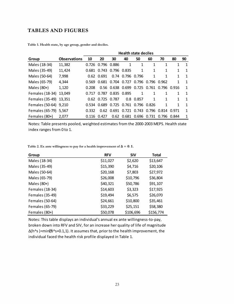
TABLES AND FIGURES

Table 1. Health state, by age group, gender and deciles.

Table 2. Ex ante willingness to pay for a health improvement of 𝚫𝚫 = 𝟎𝟎.𝟏𝟏.

Group Observations 10 20 30 40 50 60 70 80 90Males (18-34) 11,382 0.726 0.796 0.886 1 1 1 1 1 1Males (35-49) 11,424 0.681 0.743 0.796 0.835 1 1 1 1 1Males (50-64) 7,998 0.62 0.691 0.74 0.796 0.796 1 1 1 1Males (65-79) 4,344 0.569 0.681 0.704 0.727 0.796 0.796 0.962 1 1Males (80+) 1,120 0.208 0.56 0.638 0.699 0.725 0.761 0.796 0.916 1Females (18-34) 13,049 0.717 0.787 0.835 0.895 1 1 1 1 1Females (35-49) 13,351 0.62 0.725 0.787 0.8 0.857 1 1 1 1Females (50-64) 9,210 0.534 0.689 0.725 0.761 0.796 0.826 1 1 1Females (65-79) 5,567 0.332 0.62 0.691 0.721 0.743 0.796 0.814 0.971 1Females (80+) 2,077 0.116 0.427 0.62 0.681 0.696 0.731 0.796 0.844 1

Notes: Table presents pooled, weighted estimates from the 2000-2003 MEPS. Health state index ranges from 0 to 1.

Health state deciles

Group RFV SIV TotalMales (18-34) $11,027 $2,620 $13,647Males (35-49) $15,390 $4,716 $20,106Males (50-64) $20,168 $7,803 $27,972Males (65-79) $26,008 $10,796 $36,804Males (80+) $40,321 $50,786 $91,107Females (18-34) $14,603 $3,323 $17,925Females (35-49) $19,494 $6,575 $26,070Females (50-64) $24,661 $10,800 $35,461Females (65-79) $33,229 $25,151 $58,380Females (80+) $50,078 $106,696 $156,774

Notes: This table displays an individual's annual ex ante willingness-to-pay, broken down into RFV and SIV, for an increase her quality of life of magnitude Δ(h^s )=min(h^s+0.1,1). It assumes that, prior to the health improvement, the individual faced the health risk profile displayed in Table 1.

23

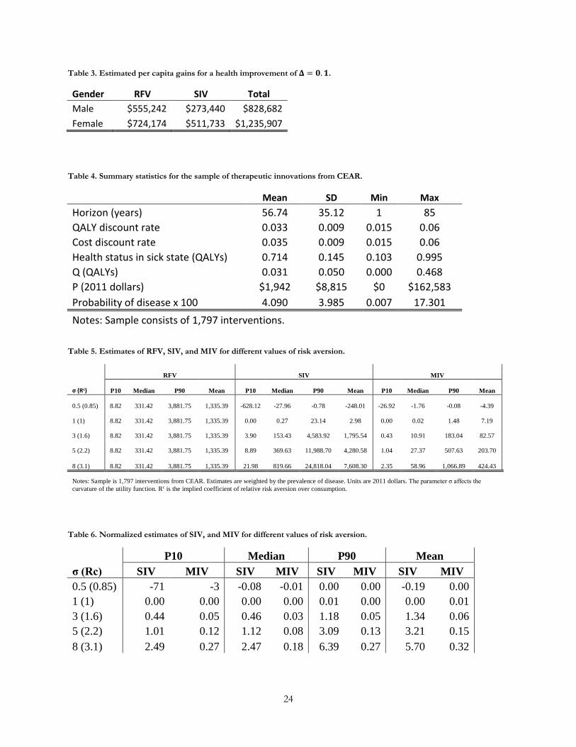
Table 3. Estimated per capita gains for a health improvement of 𝚫𝚫 = 𝟎𝟎.𝟏𝟏.

Gender RFV SIV Total Male $555,242 $273,440 $828,682 Female $724,174 $511,733 $1,235,907

Table 4. Summary statistics for the sample of therapeutic innovations from CEAR.

Mean SD Min Max Horizon (years) 56.74 35.12 1 85 QALY discount rate 0.033 0.009 0.015 0.06 Cost discount rate 0.035 0.009 0.015 0.06 Health status in sick state (QALYs) 0.714 0.145 0.103 0.995 Q (QALYs) 0.031 0.050 0.000 0.468 P (2011 dollars) $1,942 $8,815 $0 $162,583 Probability of disease x 100 4.090 3.985 0.007 17.301 Notes: Sample consists of 1,797 interventions.

Table 5. Estimates of RFV, SIV, and MIV for different values of risk aversion.

RFV SIV MIV

σ (Rc) P10 Median P90 Mean P10 Median P90 Mean P10 Median P90 Mean

0.5 (0.85) 8.82 331.42 3,881.75 1,335.39 -628.12 -27.96 -0.78 -248.01 -26.92 -1.76 -0.08 -4.39

1 (1) 8.82 331.42 3,881.75 1,335.39 0.00 0.27 23.14 2.98 0.00 0.02 1.48 7.19

3 (1.6) 8.82 331.42 3,881.75 1,335.39 3.90 153.43 4,583.92 1,795.54 0.43 10.91 183.04 82.57

5 (2.2) 8.82 331.42 3,881.75 1,335.39 8.89 369.63 11,988.70 4,280.58 1.04 27.37 507.63 203.70

8 (3.1) 8.82 331.42 3,881.75 1,335.39 21.98 819.66 24,818.04 7,608.30 2.35 58.96 1,066.89 424.43

Notes: Sample is 1,797 interventions from CEAR. Estimates are weighted by the prevalence of disease. Units are 2011 dollars. The parameter σ affects the curvature of the utility function. Rc is the implied coefficient of relative risk aversion over consumption.

Table 6. Normalized estimates of SIV, and MIV for different values of risk aversion.

P10 Median P90 Mean

σ (Rc) SIV MIV SIV MIV SIV MIV SIV MIV 0.5 (0.85) -71 -3 -0.08 -0.01 0.00 0.00 -0.19 0.00 1 (1) 0.00 0.00 0.00 0.00 0.01 0.00 0.00 0.01 3 (1.6) 0.44 0.05 0.46 0.03 1.18 0.05 1.34 0.06 5 (2.2) 1.01 0.12 1.12 0.08 3.09 0.13 3.21 0.15 8 (3.1) 2.49 0.27 2.47 0.18 6.39 0.27 5.70 0.32

24

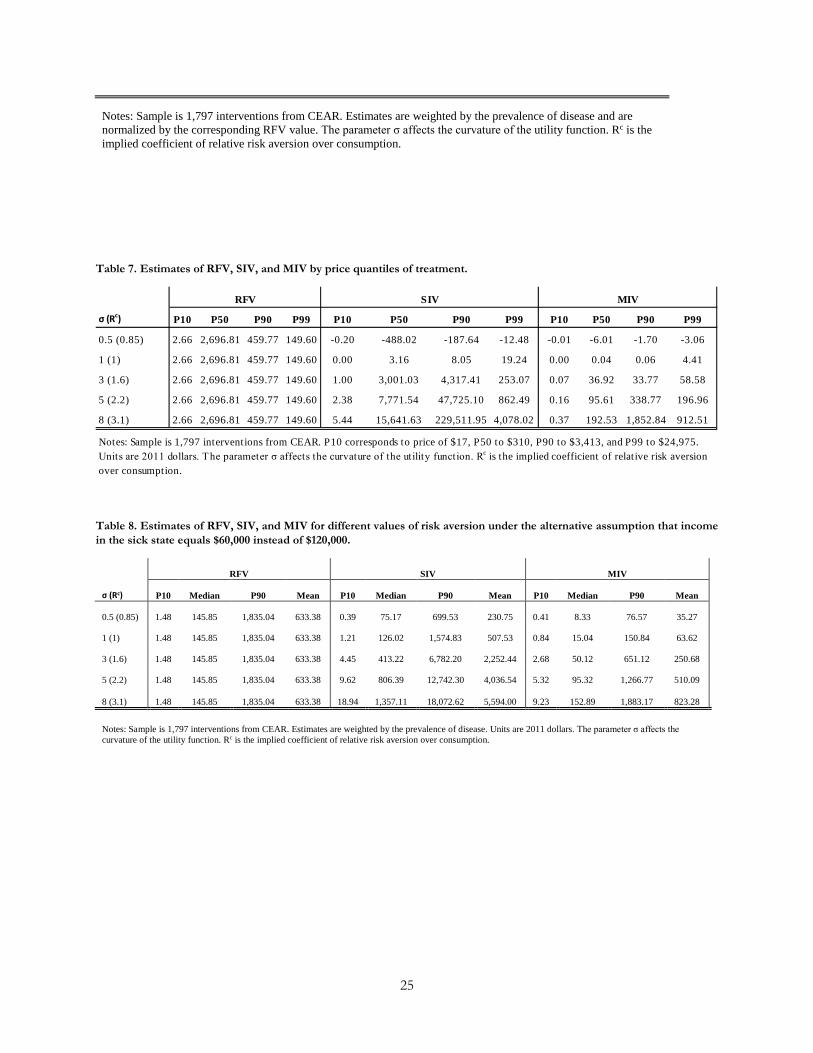
Notes: Sample is 1,797 interventions from CEAR. Estimates are weighted by the prevalence of disease and are normalized by the corresponding RFV value. The parameter σ affects the curvature of the utility function. Rc is the implied coefficient of relative risk aversion over consumption.

Table 7. Estimates of RFV, SIV, and MIV by price quantiles of treatment.

Table 8. Estimates of RFV, SIV, and MIV for different values of risk aversion under the alternative assumption that income in the sick state equals $60,000 instead of $120,000.

RFV SIV MIV

σ (Rc) P10 Median P90 Mean P10 Median P90 Mean P10 Median P90 Mean

0.5 (0.85) 1.48 145.85 1,835.04 633.38 0.39 75.17 699.53 230.75 0.41 8.33 76.57 35.27

1 (1) 1.48 145.85 1,835.04 633.38 1.21 126.02 1,574.83 507.53 0.84 15.04 150.84 63.62

3 (1.6) 1.48 145.85 1,835.04 633.38 4.45 413.22 6,782.20 2,252.44 2.68 50.12 651.12 250.68

5 (2.2) 1.48 145.85 1,835.04 633.38 9.62 806.39 12,742.30 4,036.54 5.32 95.32 1,266.77 510.09

8 (3.1) 1.48 145.85 1,835.04 633.38 18.94 1,357.11 18,072.62 5,594.00 9.23 152.89 1,883.17 823.28

Notes: Sample is 1,797 interventions from CEAR. Estimates are weighted by the prevalence of disease. Units are 2011 dollars. The parameter σ affects the curvature of the utility function. Rc is the implied coefficient of relative risk aversion over consumption.

σ (Rc) P10 P50 P90 P99 P10 P50 P90 P99 P10 P50 P90 P99

0.5 (0.85) 2.66 2,696.81 459.77 149.60 -0.20 -488.02 -187.64 -12.48 -0.01 -6.01 -1.70 -3.06

1 (1) 2.66 2,696.81 459.77 149.60 0.00 3.16 8.05 19.24 0.00 0.04 0.06 4.41

3 (1.6) 2.66 2,696.81 459.77 149.60 1.00 3,001.03 4,317.41 253.07 0.07 36.92 33.77 58.58

5 (2.2) 2.66 2,696.81 459.77 149.60 2.38 7,771.54 47,725.10 862.49 0.16 95.61 338.77 196.96

8 (3.1) 2.66 2,696.81 459.77 149.60 5.44 15,641.63 229,511.95 4,078.02 0.37 192.53 1,852.84 912.51

RFV SIV MIV

Notes: Sample is 1,797 interventions from CEAR. P10 corresponds to price of $17, P50 to $310, P90 to $3,413, and P99 to $24,975. Units are 2011 dollars. The parameter σ affects the curvature of the utility function. Rc is the implied coefficient of relative risk aversion over consumption.

25

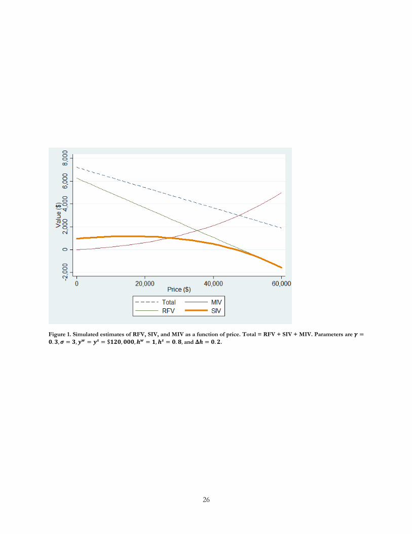
Figure 1. Simulated estimates of RFV, SIV, and MIV as a function of price. Total = RFV + SIV + MIV. Parameters are 𝜸𝜸 =𝟎𝟎.𝟑𝟑,𝝈𝝈 = 𝟑𝟑,𝒚𝒚𝒘𝒘 = 𝒚𝒚𝒔𝒔 = $𝟏𝟏𝟏𝟏𝟎𝟎,𝟎𝟎𝟎𝟎𝟎𝟎,𝒉𝒉𝒘𝒘 = 𝟏𝟏,𝒉𝒉𝒔𝒔 = 𝟎𝟎.𝟖𝟖, and 𝚫𝚫𝒉𝒉 = 𝟎𝟎.𝟏𝟏.

26

Figure 2. This figure displays the distribution of ∆𝒉𝒉, a measure of health improvement that ranges from 0 to 1, in our therapeutic innovation sample.

27

Figure 3. This figure displays the distribution of prices for the treatments in our therapeutic innovation sample. Price is top-coded at $50,000 for display purposes.

Figure 4. Distribution of the risk-free value (RFV) in the CEAR sample of therapeutic technologies.

28

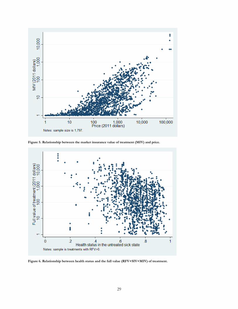
Figure 5. Relationship between the market insurance value of treatment (MIV) and price.

Figure 6. Relationship between health status and the full value (RFV+SIV+MIV) of treatment.

29

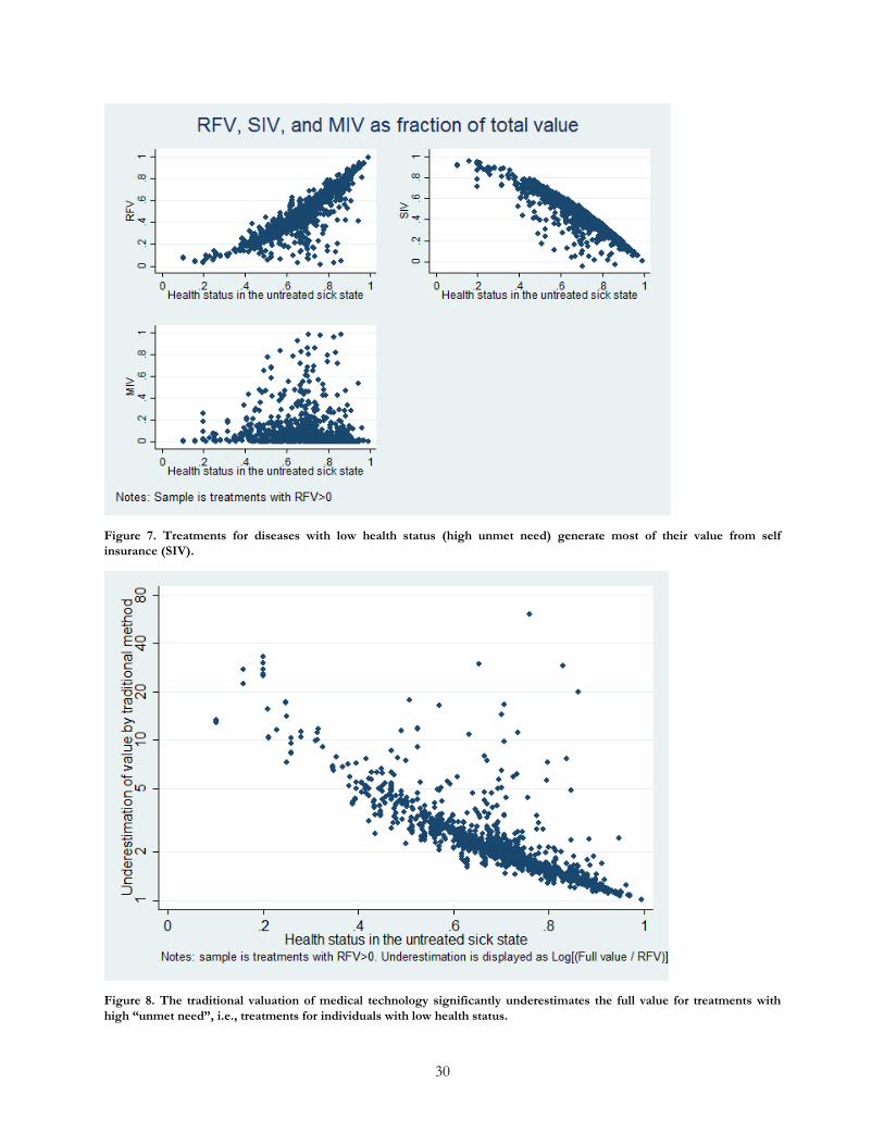
Figure 7. Treatments for diseases with low health status (high unmet need) generate most of their value from self insurance (SIV).

Figure 8. The traditional valuation of medical technology significantly underestimates the full value for treatments with high “unmet need”, i.e., treatments for individuals with low health status.

30

31

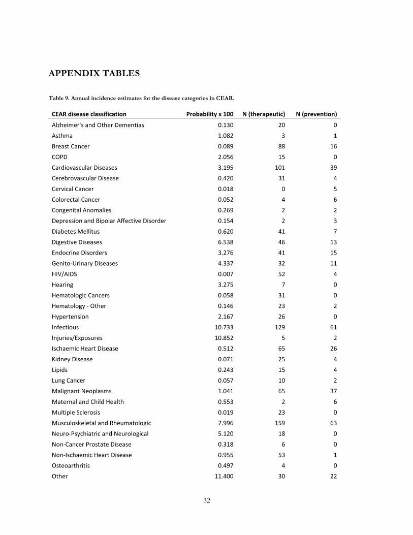
APPENDIX TABLES

Table 9. Annual incidence estimates for the disease categories in CEAR.

CEAR disease classification Probability x 100 N (therapeutic) N (prevention)

Alzheimer's and Other Dementias 0.130 20 0 Asthma 1.082 3 1

Breast Cancer 0.089 88 16 COPD 2.056 15 0 Cardiovascular Diseases 3.195 101 39 Cerebrovascular Disease 0.420 31 4

Cervical Cancer 0.018 0 5 Colorectal Cancer 0.052 4 6 Congenital Anomalies 0.269 2 2 Depression and Bipolar Affective Disorder 0.154 2 3

Diabetes Mellitus 0.620 41 7 Digestive Diseases 6.538 46 13 Endocrine Disorders 3.276 41 15 Genito-Urinary Diseases 4.337 32 11

HIV/AIDS 0.007 52 4 Hearing 3.275 7 0 Hematologic Cancers 0.058 31 0 Hematology - Other 0.146 23 2

Hypertension 2.167 26 0 Infectious 10.733 129 61 Injuries/Exposures 10.852 5 2 Ischaemic Heart Disease 0.512 65 26

Kidney Disease 0.071 25 4 Lipids 0.243 15 4 Lung Cancer 0.057 10 2 Malignant Neoplasms 1.041 65 37

Maternal and Child Health 0.553 2 6 Multiple Sclerosis 0.019 23 0 Musculoskeletal and Rheumatologic 7.996 159 63 Neuro-Psychiatric and Neurological 5.120 18 0

Non-Cancer Prostate Disease 0.318 6 0 Non-Ischaemic Heart Disease 0.955 53 1 Osteoarthritis 0.497 4 0 Other 11.400 30 22

32

Other Endocrine 3.217 9 6 Other Genito-Urinary 4.034 2 0 Other Infectious Diseases 9.822 39 12 Other Musculoskeletal 6.478 38 3

Other Neoplasms 1.696 14 10 Other Neuro-Psychiatric and Neurological 4.904 5 5 Other Non-Infectious GI Diseases 6.443 26 5 Other Respiratory 1.981 12 1

Ovary Cancer 0.007 4 3 Parkinson Disease 0.031 3 0 Peptic Ulcer Disease 0.152 2 0 Prostate Cancer 0.106 15 3

Respiratory Diseases 17.301 8 6 Respiratory Infections 15.130 2 0 Rheumatoid Arthritis 0.141 21 4 STDs excluding HIV 1.305 1 6

Schizophrenia 0.029 3 0 Seizure Disorders (Epilepsy) 0.032 10 0 Sense Organ Diseases 6.806 0 5 Skin Diseases (Non-Cancer) 4.614 7 2

Substance Abuse Disorders 0.213 6 1 Tuberculosis 0.020 4 3 Vascular, Non-Cardiac, Non-Cerebral 1.030 30 2 Vision 4.021 46 4

Total 1,481 437

Source: 1996-2010 MEPS surveys.

33