The information content of over-the-counter currency options

WORK ING PAPER S ER I E SNO. 366 / J UNE 2004

THE INFORMATIONALCONTENT OF OVER-THE-COUNTERCURRENCY OPTIONS

by Peter Christoffersen and Stefano Mazzotta

In 2004 all publications

will carry a motif taken

from the €100 banknote.

WORK ING PAPER S ER I E SNO. 366 / J UNE 2004

THE INFORMATIONAL CONTENT OF

OVER-THE-COUNTER CURRENCY OPTIONS 1

by Peter Christoffersen 2

and Stefano Mazzotta 3

1 We have benefited from several visits to the External Division of the European Central Bank whose hospitality is gratefully acknowledged. Veryuseful comments were provided by Torben Andersen, Lorenzo Cappiello, Olli Castren, Bruce Lehmann, Filippo di Mauro, Stelios Makrydakis,

Nour Meddahi and Neil Shephard. The OTC volatilities used in this paper were provided by Citibank N.A.The usual disclaimer applies.2 McGill University, CIRANO and CIREQ McGill University: [email protected].

3 McGill University.

This paper can be downloaded without charge from http://www.ecb.int or from the Social Science Research Network

electronic library at http://ssrn.com/abstract_id=533126.

© European Central Bank, 2004

AddressKaiserstrasse 2960311 Frankfurt am Main, Germany

Postal addressPostfach 16 03 1960066 Frankfurt am Main, Germany

Telephone+49 69 1344 0

Internethttp://www.ecb.int

Fax+49 69 1344 6000

Telex411 144 ecb d

All rights reserved.

Reproduction for educational and non-commercial purposes is permitted providedthat the source is acknowledged.

The views expressed in this paper do notnecessarily reflect those of the EuropeanCentral Bank.

The statement of purpose for the ECBWorking Paper Series is available from theECB website, http://www.ecb.int.

ISSN 1561-0810 (print)ISSN 1725-2806 (online)

3ECB

Work ing Paper Ser ie s No . 366June 2004

CONTENT S

Abstract 4

Non-technical summary 5

1 Introduction 7

2 Volatility forecast evaluation 9

3 Volatility forecast evaluation results 12

4 Interval forecast evaluation 15

5 Density forecast evaluation 18

5a Graphical density forecast evaluation 19

5b Tests of the unconditional normaldistribution 20

5c Tests of the conditional normaldistribution 22

6 Conclusion and directions for future work 23

References 25

Figures 28

Tables 36

European Central Bank working paper series 47

Abstract

Financial decision makers often consider the information in currency option valuations when

making assessments about future exchange rates. The purpose of this paper is to systematically

assess the quality of option based volatility, interval and density forecasts. We use a unique

dataset consisting of over 10 years of daily data on over-the-counter currency option prices. We

find that the OTC implied volatilities explain a much larger share of the variation in realized

volatility than previously found using market-traded options. Finally, we find that wide-range

interval and density forecasts are often misspecified whereas narrow-range interval forecasts are

well specified.

JEL Classifications: G13, G14, C22, C53

Keywords: FX, Volatility, Interval, Density, Forecasting

4ECBWork ing Paper Ser ie s No . 366June 2004

Non-Technical Summary

Financial decision makers often consider the forward-looking information in currency

option valuations when making assessments about future developments in foreign exchange

rates. Option implied volatilities can be used as forecasts of realised volatility and interval and

density forecasts can be extracted from strangles and risk-reversals. The purpose of this paper is

to assess the quality of such volatility, interval and density forecasts. Our work is based on a very

unique database consisting of more than ten years of daily quotes on European currency options

from the OTC market. The OTC quotes include at-the-money implied volatilities, strangles and

risk-reversals on the dollar, yen and pound per euro as well as on the yen per dollar. From this

data we have constructed daily 1-month interval and density forecasts using the methodology in

Malz (1997).

The main findings of the paper are as follows: First and foremost, we find that the OTC

implied volatilities explain a much larger share of the variation in realized volatility than has

been found previously in studies relying on market-traded options. Second, we find that wide-

range interval forecasts are often misspecified whereas narrow-range interval forecasts are well

specified. Third, we find that the option-based density forecasts are rejected in general. Graphical

inspection of the density forecasts suggests that while the sources of rejections vary from

currency to currency misspecification of the distribution tails is a common source of error.

Our paper contributes in two areas of the literature. First, to our knowledge, the empirical

performance of option-based interval and density forecasts has not been systematically explored

so far. Second, while there is a considerable literature on implied volatility forecasts from

market-traded options, OTC data have only recently been employed.

One of our contributions consists of analyzing a unique dataset of OTC options which

turns out to have impressive volatility prediction properties. OTC options are quoted daily with a

fixed maturity (say one month) whereas market-traded options have rolling maturities which in

turn complicate their use in fixed-horizon volatility forecasting.

In addition to volatility forecasts we evaluate option-based interval and density forecasts

which are widely used by practitioners but which have not been systematically assessed so far.

OTC options are quoted daily with fixed moneyness in contrast with market-traded options

which have fixed strike prices and thus time-varying moneyness as the spot price changes. This

time-varying moneyness complicates the use of market-traded options for interval and density

forecasting in that the effective support of the distribution is changing over time. Finally, the

5ECB


trading volume in OTC options is often much larger than in the corresponding market traded

contracts which in turn is likely to render the OTC quotes more reliable for information

extraction.

Several promising directions for future research exist. First, policy makers may be

interested in assessing speculative pressures on a given exchange rate. The option implied

densities can be used in this regard by constructing daily option-implied probabilities of say a

3% appreciation or depreciation during the next month. Second, the accuracy of the left and right

tail interval forecast could be analyzed separately in order to gain further insight on the

probability of a sizable appreciation or depreciation. Third, relying on the triangular arbitrage

condition linking the JPY/EUR, the USD/EUR, and the JPY/USD, one can construct option

implied covariances and correlations from the option implied volatilities. These implied

covariances can then be used to forecast realized covariances as done for volatilities in Tables 1-

4. Fourth, the misspecification found in the option-implied density forecasts may be rectified by

assuming different tail-shapes in the density estimation or by incorporating return-based

information. Converting the risk-neutral densities to their statistical counterparts may be useful

as well but will require further assumptions, which may or may not be empirically valid. Bliss

and Panigirtzoglou (2004) present promising results in this direction. Finally, one could consider

making density forecasts combining option-implied and return based densities. We leave these

important issues for future work.


1. Introduction

Financial decision makers often consider the forward-looking information in currency

option valuations when making assessments about future developments in foreign exchange

rates.1 Option implied volatilities can be used as forecasts of realised volatility and interval and

density forecasts can be extracted from strangles and risk-reversals. The purpose of this paper is

to assess the quality of such volatility, interval and density forecasts. Our work is based on a very

unique database consisting of more than ten years of daily quotes on European currency options

from the OTC market.2 The OTC quotes include at-the-money implied volatilities, strangles and

risk-reversals on the dollar, yen and pound per euro3 as well as on the yen per dollar. From this

data we have constructed daily 1-month interval and density forecasts using the methodology in

Malz (1997).

The main findings of the paper are as follows: First and foremost, we find that the OTC

implied volatilities explain a much larger share of the variation in realized volatility than has

been found previously in studies relying on market-traded options. Second, we find that wide-

range interval forecasts are often misspecified whereas narrow-range interval forecasts are well

specified. Third, we find that the option-based density forecasts are rejected in general. Graphical

inspection of the density forecasts suggests that while the sources of rejections vary from

currency to currency misspecification of the distribution tails is a common source of error.

Several early contributions use market-based options data with mixed results. Beckers

(1981) finds that not all available information is reflected in the current option price and question

the efficiency of the option markets. Canina and Figlewski (1993) find implied volatility to be a

poor forecast of subsequent realized volatility. Lamoureux and Lastrapes (1993) provide

evidence against restrictions of option pricing models which assume that variance risk is not

priced. Jorion (1995) finds that statistical models of volatility based on returns are outperformed

by implied volatility forecasts even when the former are given the advantage of ex post in sample

parameter estimation. He also finds evidence of bias. More recently, Christensen and Prabhala

(1998) using longer time series and non overlapping data find that implied volatility outperforms

1

(2002), and OECD (1999). 2 The OTC volatilities used in this paper were provided by Citibank N.A 3 Prior to January 1, 1999 these were denoted in DEM.

7ECB


See for example Bank for International Settlements (2003), Bank of England (2000), International Monetary Fund

past volatility in forecasting future volatility. Fleming (1998) finds that implied volatility

dominates the historical volatility in terms of ex ante forecasting power and suggests that a linear

model which corrects for the implied volatility’s bias can provide a useful market-based

estimator of conditional volatility. Blair, Poon, and Taylor (2001), find that nearly all relevant

information is provided by the VIX index and there is not much incremental information in high-

frequency index returns. Neely (2003) finds that econometric projections supplement implied

volatility in out-of-sample forecasting and delta hedging. He also provides some explanations for

the bias and inefficiency pointing to autocorrelation and measurement error in implied volatility.

In work concurrent with ours, Pong, Shackleton, Taylor and Xu (2004) find that high-

frequency historical forecasts are superior to implied volatilities using OTC data for horizons up

to one week. Covrig and Low (2003) use OTC data to find that quoted implied volatility

subsumes the information content of historically based forecasts at shorter horizons, and the

former is as good as the latter at longer horizons.

Our paper contributes in two areas of the literature. First, to our knowledge, the empirical

performance of option-based interval and density forecasts has not been systematically explored

so far. Second, while there is a considerable literature on implied volatility forecasts from

market-traded options, OTC data have only recently been employed.

One of our contributions consists of analyzing a unique dataset of OTC options which

turns out to have impressive volatility prediction properties. OTC options are quoted daily with a

fixed maturity (say one month) whereas market-traded options have rolling maturities which in

turn complicate their use in fixed-horizon volatility forecasting.

In addition to volatility forecasts we evaluate option-based interval and density forecasts

which are widely used by practitioners but which have not been systematically assessed so far.

OTC options are quoted daily with fixed moneyness in contrast with market-traded options

which have fixed strike prices and thus time-varying moneyness as the spot price changes. This

time-varying moneyness complicates the use of market-traded options for interval and density

forecasting in that the effective support of the distribution is changing over time. Finally, the

trading volume in OTC options is often much larger than in the corresponding market traded

contracts which in turn is likely to render the OTC quotes more reliable for information

extraction.

The remainder of the paper is structured as follows. Section 2 defines the competing

volatility forecasts we consider and describes the standard regression-based framework for


volatility forecast evaluation. Section 3 presents results on the option-implied and historical

return-based volatility forecasts of realized volatility. Section 4 suggests a method for evaluating

interval forecasts from option prices and present results from this method. Section 5 suggests

methods for evaluating density forecasts from option prices and present results from these

methods. Finally, Section 6 discusses potential points for future research.

2. Volatility Forecast Evaluation

In order to evaluate the informational content of the volatilities implied from currency

options, we define the realized4 future volatility for the next h days to be

h

iit

RVht R

h 1

2,

252

in annualized terms, where Rt+i = ln(St+i/St+i-1) is the FX spot return on day t+i. This realized

volatility (and its logarithm) will be our forecasting object of interest in this section.5

We will consider four competing forecasts of realized volatility. First and most importantly

the implied volatility from at-the-money OTC currency options with maturity h, where h is either

1 month or 3 months corresponding to roughly 21 and 63 trading days respectively. Denote this

options-implied volatility by IVht , .

The other three volatility forecasts are derived from historical FX returns only. The

simplest possible forecast is the historical h-day volatility, defined as

RVhht

h

iiht

HVht R

h ,1

2,

252

The historical volatility is a simple equal weighted average of past squared returns.

We can instead consider volatilities that apply an exponential weighting scheme putting

progressively less weight on distant observations. The simplest such volatility is the Exponential

Smoother or RiskMetrics volatility, where daily variance evolves as

22

1

21

121 1~1~

tti

iti

t RR

4 See Andersen, T., T. Bollerslev, F. X. Diebold, and P. Labys, 2003. 5 Later on we will consider realized volatilities calculated from 30-minute rather than daily returns.

9ECB


Following JP Morgan we simply fix =0.94 for all the daily FX returns. The fact that the

coefficients on past variance and past squared returns sum to one makes this model akin to a

random walk in variance. The annualized forecast for h-day volatility is therefore simply

21,

~252 tRMht

Finally we consider a simple, symmetric GARCH(1,1) model, where the daily variance

evolves as222

1 ˆˆ ttt R

In contrast with the RiskMetrics model, the GARCH model implies a non-constant term structure

of volatility. The unconditional variance in the model can be computed as

1ˆ 2

The conditional variance for day t+h can be derived as 22

1122

| ˆˆˆˆ th

tht

And the annualized GARCH volatility forecast for day t+1 through t+h is thus

h

it

iGHht h 1

221

12, ˆˆˆ252

The GARCH model will have a downward sloping volatility term structure when the current

variance is above the long horizon variance and vice versa.6

Notice that while we take the standard approach of estimating a daily volatility model to

forecast monthly and quarterly volatility, this is not the only way to proceed. Ghysels, Santa-

Clara and Valkanov (2003) have recently explored ways to estimate volatility forecasting models

directly on the relevant horizon of interest. Rather than estimating say a monthly forecasting

model on monthly data they make use of the information in daily observations in a horizon-

specific forecasting model imposing a parsimonious lag structure on the daily observations.

Figure 1 shows the spot rates of the four FX rates analysed in this paper. Prior to the euro

introduction in 1999 we observe FX options denoted against the Deutschmark (DEM) and we

6 The GARCH model contains parameters which must be estimated. We do this on rolling 10-year samples starting

in January 1982 and using QMLE. Each year we forecast volatility one-year out-of-sample before updating the

estimation sample by another calendar year of daily returns. The euro volatility forecasts are constructed using

synthetic euro rates in the period prior to the introduction of the euro.


will therefore work with the DEM spot rates prior to the euro introduction as well. Prior to

January 1, 1999 we use DEM options to forecast DEM volatility and afterwards we use euro

options to forecast euro volatility.

The five volatility specifications including the realized volatility are plotted in Figures 2-5.

Each page corresponds to a particular volatility specification and each column on a page

represents an FX rate. The top row shows the 1-month volatility and the bottom row the 3-month

volatility. Notice that the RiskMetrics volatilities in Figure 4 are identical for 1-month and 3-

month maturities as the random-walk nature of this specification implies a flat volatility term

structure.

We are now ready to assess the quality of the different volatility forecasts. This will be

done in simple linear predictability regressions. We first run four univariate regressions for each

currency

GH,RM,HV,IVjfor,ba jh,t

jh,t

RVh,t

The purpose of these univariate regressions is to assess the fit through the adjusted R2 and to

check how close the estimates of a are to 0 and how close the estimate of b are to 1. Bollerslev

and Zhou (2003)7 point out that if the volatility risk is priced in the options markets then we

should expect to find a positive intercept and a slope less than one in the above regression. In a

standard stochastic volatility set up, it can be shown that if the price of volatility risk is zero, the

process followed by the volatility is identical under the objective and the risk neutral measures.

In such a case there would be no bias. However, the volatility risk premium is generally

estimated to be negative which in turn implies that the volatility process under the risk neutral

measure will have higher drift. This is also consistent with the fact that implied volatilities are

empirically found to be upward biased estimates of the objective volatility.

Aside these considerations, for someone using implied volatility in the real time

monitoring of FX movements, the intercept and slope coefficients are informative of the size of

the bias and efficiency respectively of the forecasts.

In addition we will run three bivariate regressions including the implied volatility forecast

as well as each of the three return-based volatility forecasts in turn. Thus we have

GH,RM,HVjfor,cba j,IVh,t

jh,t

IVh,t

RVh,t

7 See also Bandi and Perron (2003), Chernov (2003), Bates (2002), and Benzoni (2001).

11ECB


The purpose of the bivariate regressions is to assess if the return-based volatility forecasts add

anything to the market-based forecasts implied from currency options.

Finally, we run a regression including all the four volatility forecasts in the same equation.

The purpose of this regression is to assess the relative merits of the different volatility forecasts.

We will run all regressions for h=21 and 63 corresponding to the 1-month and 3-month

option maturities. We will also run all regressions in levels of volatility as above as well as in

logarithms. Due to the volatilities being strictly positive, the log specification may have error

terms, which are better behaved than those from the level regressions.

3. Volatility Forecast Evaluation Results

Tables 1 and 2 report the regression point estimates as well as standard errors corrected for

heteroskedasticity and autocorrelation. Throughout this paper we apply GMM using the Newey-

West8 weighting matrix with a prespecified bandwidth equal to 21 days for the 1-month horizon

(Table 1) and 63 days for the 3-month horizon (Table 2). The bandwidth is chosen as to

eliminate the influence of the autocorrelation induced by the overlapping observation. We also

report the regression fit using the adjusted R2.

Several strong and interesting empirical regularities emerge. First, the regression fit is very

good in all cases. Jorion (1995) reports R2 in the region 0.10-0.15 for the USD/JPY, USD/DEM

and USD/CHF using implied volatility forecasts. We get instead R2 of 0.30-0.38 for the 1-month

maturity and 0.16-0.35 for the 3-month maturity case. Second, comparing the R2 across the

univariate forecast regressions we see that the implied volatility is the best volatility forecast.

This result holds across currencies and horizons.

Third, comparing the slope estimates across the bivariate forecast regressions where the

implied volatility forecast is included along with each of the other three forecasts, the implied

volatility always has the highest slope. Thus, in the cases when GARCH has a higher slope in the

univariate regression the bivariate regressions including the IV and GARCH forecasts always

assign a larger slope to the IV forecast. The fact that GARCH-based forecasts sometimes have a

slope closer to one than do the implied volatility forecasts is not surprising given the price of

8 See Newey and West (1987).


volatility risk argument in Bollerslev and Zhou (2003) and others.9 Nevertheless, it is interesting

to note that the R2 is higher for the implied volatility forecasts even in the cases where its slope is

lower than that of the GARCH-based forecasts.

Fourth, comparing the slope estimates across the multivariate forecast regressions where

all four forecasts are included simultaneously the implied volatility has the highest slope. This

result holds across currencies and horizons. Fifth, comparing across the horizon forecasts it

appears perhaps not surprisingly that the 1-month forecasts have higher R2 than the 3-month

forecasts. Finally, the slope coefficient is often insignificantly different from one for the IV

forecasts, and its intercept is often insignificantly different from zero.

Tables 3 and 4 contain the same set of regressions as Tables 1 and 2, but now run on the

euro sample (i.e. post January 1, 1999) only, and furthermore relying on 30-minute intraday

returns rather than daily returns to compute the one and three month realized volatilities. We also

report the euro sample estimates using daily data in Table 3a and 4a.

The objective of Tables 3 and 4 is to see if the post-euro sample is different from the full

sample period which straddles the introduction, and furthermore to assess the value of using

high-frequency returns in volatility forecast evaluation. The theoretical benefits of doing so have

been documented in Andersen and Bollerslev (1998) and Andersen, Bollerslev and Meddahi

(2003) who show that the R2 in the regressions we run will be significantly higher when

proxying for true volatility using an intraday rather than daily return-based volatility measure. As

pointed out by Alizadeh, Brandt and Diebold (2002), and Brandt and Diebold (2003) this

theoretical benefit may in practice be outweighed by market microstructure noise, but relying on

30-minutes returns in very liquid markets as we do here should mitigate these problems.

The results in Table 3 and 4 are broadly similar to those from the full sample but using

high-frequency returns does lead to some new interesting findings. First, for the three euro cross

currencies the regression fit is typically much better now. Due to the obvious structural break in

1999 this is perhaps not surprising. But it is still interesting that we now get R2 as high as 65% in

the univariate regressions. Note that the R2 for the 3-month JPY/USD case is now slightly lower

than before. It is therefore not simply the case the FX volatility has become more predictable as

of late.

9 Whether volatility risk is priced is of course an empirical question: some of our results indirectly support the

conjecture that volatility risk is priced in the currency options markets.

13ECB


Second, comparing the R2 across the univariate forecast regressions the implied volatility is

typically the best volatility forecast.10 The exception is the EUR/JPY rate. Third, comparing the

slope estimates across the bivariate and multivariate forecast regressions the implied volatility

typically has the highest slope. It is interesting that the simple historical realized volatility

forecast now sometimes has the highest slope.11 This is results is exclusively due to the use of

high frequency data as it is easy to infer from the comparison of Table 3-4 to 3a-4a. The added

accuracy in this forecast from the intra-day returns is thus evident.

In order to give assess the importance of the choice of estimation period we have also run

the same regressions using in sample GARCH estimates.12 Although the explanatory power as

measured by the adjusted R2 of the in sample GARCH is substantially higher compared to that of

the out of sample regressions, in most cases the change does not affect the results in the 1-month

regressions for any currency both in the full sample and in the post 1999 sample. The same is

true for the 3-month horizon with the only exception of the GBP in the full sample: here the in

sample GARCH get the highest coefficient in the multivariate regression.

In summary, we find strong evidence that the implied volatility from FX options is useful

in predicting future realized volatility at the one and three month horizons. The predictability is

particularly strong for the euro cross rates in the recent period. In spite of the potential bias from

volatility risk being priced in the options, the regression slope on the volatility forecasts are often

quite close to one.

Perhaps the most striking finding in Tables 1-4 is the high level of R2 found in the implied

volatility regressions. It appears that the volatility implied in the OTC options offer much more

precise forecasts than the volatility implied from market-traded options, which have been

analyzed in previous studies. We suspect that the so-called telescoping bias arising from the

rolling-maturity structure of market-traded options (see Christensen, Hansen, and Prabhala,

2001) could be part of the reason. Furthermore, the fact that OTC options are quoted daily with a

fixed moneyness, as opposed to a fixed strike price, which ensures that the options used for

11 The historical volatility forecast could potentially be improved further by estimating a slope coefficient thus

allowing for mean reversion in the forecast. 12 Results are not shown here to conserve space.


volatility forecasting are exactly at-the-money each day. Finally, the large volume of transaction

in OTC currency options compared with market traded options may offer additional explanation.

4. Interval Forecast Evaluation

The information in currency options may be useful not only for volatility forecasting but

for spot rate distribution forecasting more generally. In the following sections we abstract from

the difference between risk neutral and objective distributions. The empirical question we want

to ask is: “How well can risk neutral intervals and densities computed using standard

methodologies forecast physical interval and densities”. The legitimacy of the question stems

from the fact that financial decision makers often consider the information in currency option

valuations when making assessments about future exchange rates without worrying about this

important theoretical difference. In addition, this pragmatic approach can be justified by

considering that for currencies the risk premium, i.e. the conditional mean, which would largely

determine the difference between risk neutral and physical, may not be as important as the higher

order moments and particularly the conditional variance.13 In other words, the tests in the

following sections can be considered as joint tests of the methodology used to extract densities

and intervals under the additional hypothesis that the objective and risk neutral distributions are

not very different.14

These tests may have low power with respect to generic alternative hypotheses but they

can help assessing whether certain specific pieces of information have been duly taken into

account in the construction of these intervals and densities. Rejection may come from the

presence of some currency risk premium: this situation will shift apart the mean under the two

probabilistic measures. Rejection could also come from methodological and data shortcoming in

the construction of the interval and densities: this is likely to be the case for the widest intervals

and the tails of the distributions when they are based on the extrapolation of market data.

13 It is also the case that there is no methodology to transform risk neutral distributions into their objective

counterparts without making several, possibly very restrictive assumptions. 14 In order to save space we do not compare the predictive performance of our option implied densities with that of

densities based on historical FX returns only. This is an interesting exercise which we leave for future studies.

15ECB


In substance, the results of these tests should be seen as suggestion for improvement of the

prevalent methodologies and caveats with regard to how much trust should one put in these

forecasts.

In this section we study the performance of one-month interval forecasts calculated from

option prices and forward rates.

The intervals are constructed from the option-implied densities which in turn are calculated

using the estimation method in Malz (1997). The Malz methodology is based on a second order

Taylor approximation to the volatility smile. The procedure forces the approximation of the

implied volatility function to be exactly equal to the observed implied volatility for the three

values of the Black-Scholes delta, namely .25, .50, and .75. It uses this interpolated

approximation of the smile to compute a continuous option price function. It then uses the

classical result in Breeden and Litzenberger (1978) to compute the risk neutral density.

We have computed conditional interval forecasts for the {0.45, 0.55} probability interval,

as well as the {0.35, 0.65}, {0.25, 0.75}, {0.15, 0.85}, and the {0.05, 0.95} intervals. These

forecasts are shown in Figure 6. Notice that the intervals for the GBP/DEM look excessively

jagged in a large part of the pre euro sample.

We now set out to evaluate the usefulness of the interval forecasts following the

methodology developed first in Christoffersen (1998). Let the generic interval forecast be

defined as

)(),( , UhtLt,h pUpL

where pL and pU are the percentages associated with the lower and upper conditional quantiles

making up the interval forecast.

Consider now the indicator variable defined as

notif,1if0 )}(p),U(p{L S,

I Ut,hLt,hhtt,h

Then if the interval forecast is correctly calibrated, we must have that

pppXIE LUtht 1|,

where Xt denotes a vector of information variables (and functions thereof) available on day t. If

the interval forecast is correctly calibrated then the expected outcome of the future FX rate


falling outside the predicted interval must be a constant equal to the pre-specified interval

probability p.

This hypothesis will be tested in a linear regression setup, but binary regression methods

could have been used as well. Under the alternative hypothesis we have

httht bXapI ,,

and the null hypothesis corresponds to the restrictions

0ba

Running these regressions on daily data we again have to worry about overlapping observations,

which we allow for using GMM estimation.

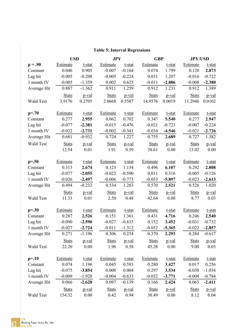
Table 5 shows the results for the regression-based tests of the interval forecasts. The

interval forecasts for the {0.45, 0.55}, {0.35, 0.65}, {0.25, 0.75}, {0.15, 0.85}, and the {0.05,

0.95} intervals are denoted by the probability of an observation outside the interval, i.e. p=.90,

.70, .50, .30 and .10 respectively. We refer to these outside observations as hits. The zero/one hit

sequence (less its expected value p) is regressed on a constant, the 21-day lagged hit and the 21-

day lagged 1-month implied volatility. The lagged hit is included to capture any dependence in

the outside observations. The implied volatility is included to assess if it is incorporated

optimally in the construction of the interval forecast. If the interval forecast is correctly specified

then the intercept and slopes should all be equal to zero. Table 5 reports coefficient estimates

along with t-statistics again calculated using GMM. Below the solid line in each subsection of

the table the average hit rate, which should be equal to p, is reported along with the t-statistic

from the test that the average hit rate indeed equals p. All t-statistics larger than two in absolute

value are denoted in boldface type. We also include Wald tests of the joint hypothesis that all the

estimated coefficients are zero.

The results in Table 5 can be summarized as follows. First, for the pound the average hit

rate is significantly different from the pre-specified p for all but the narrowest interval (with

outside probability equal to .90). The jagged pound intervals evident from Figure 6 are probably

the culprit here. Second, for the other three FX rates, the average hit rate is typically not

significantly different from the pre-specified p. The only notably exception is the wide-range

intervals (with outside probability .10) where all but the JPY/EUR intervals are rejected. It thus

appears that the interval forecast have the hardest time forecasting the tails of the spot rate

distribution.

17ECB


Third, notice that no regression slopes are significant in the JPY/EUR case. No dependence

in the hit sequence is apparent and the information in implied volatilities seems to be used

optimally in this case. Fourth, while the interval forecasts for the JPY/EUR are well specified,

the intervals for the other three forecasts are typically rejected. The slope on the 21-days lagged

implied volatility is most often found to be significantly negative. This indicates that the hits tend

to occur when the implied volatility was relatively low on the day the forecast was made. If the

intervals had been using the implied volatility information optimally then no dependence should

be found between the current implied volatility and the subsequent realization of the hit

sequence.

Table 6 reports the interval forecast evaluation results using data from the euro sample

only. The results are now somewhat different and can be summarized as follows. First, the

average hit rate is typically not significantly different from the pre-specified p with a couple of

noteworthy exceptions: The average hit rate is rejected across all the four FX rates for the widest

intervals. Again, it appears that the option implied densities have trouble capturing the tails of

the distribution. For all four FX rates it is the case that the outside hit frequency is lower than it

should be, thus the wide-range option-implied intervals are too wide on average.

Second, the average hit rate is rejected in the two widest intervals for the pound, but in

general the pound intervals are better calibrated in the euro sample than before. Third, the

JPY/USD interval is now the most poorly calibrated interval.

In summary we find that the option-implied interval forecast for the euro cross rates

perform well in the post January 1, 1999 sample. The exception is the forecasts for the widest

intervals, which tend to be too wide on average. The option-implied densities apparently have

trouble capturing the tail behaviour of the spot rate distributions. The rejection of widest

intervals and thus misspecification of the tails of the density forecasts should perhaps not come

as a surprise. The density tails are estimated on the basis of an extrapolation of the volatility

smile from the values for which option price information is available (that is for deltas equal to

.25, .50, and .75). It appears that this extrapolation could be improved. We will pursue the topic

of density forecasting in more detail in the next section.

5. Density Forecast Evaluation

The option-implied interval forecasts analyzed above are constructed from the implied

density, which contains much more information than the intervals alone. We would therefore like


to evaluate the appropriateness of these density forecasts in their own right. Doing so is likely to

yield some insights into the poor performance of the widest interval forecasts, which was noted

above. We start off by outlining the general ideas behind density forecast evaluation developed

by Diebold, Gunther and Tay (1998).

Let SF ht , and Sf ht , denote the cumulative and probability density function forecasts

made on day t for the FX spot rate on day t+h. We can then define the so-called probability

transform variable as

.)( ,,, hthththt SFduufUhtS

The transform variable captures the probability of obtaining a spot rate lower than the realization

where the probability is calculated using the density forecast. The probability will of course take

on values in the interval [0,1]. If the density forecast is correctly calibrated then we should not be

able to predict the value of the probability transform variable Ut,h using information available at

time t. That is we should not be able to forecast the probability of getting a value smaller than the

realization. Moreover, if the density forecast is a good forecast of the true probability distribution

then the estimated probability will be uniformly distributed on the [0,1] interval.

5.a Graphical Density Forecast Evaluation

Figure 7 assesses the unconditional distribution of the probability transform variable Ut,h

for each spot rate through a simple histogram. If the density forecast is correctly calibrated then

each of the histograms should be roughly flat and a random 10% of the 31 bars should fall

outside the two horizontal lines delimiting the 90% confidence band.

It appears that the histograms display certain systematic differences from the uniform

distribution. Notice in particular that the JPY/EUR histogram (top right panel) shows a

systematically declining shape moving from left to right. This is indicative of the forecasted

mean spot rate being wrong. There are too many observations where the realized spot rate lies in

the left side of the forecasted distribution (and generates a Ut,h less than 0.5) and vice versa. In

the USD/EUR case (top left panel) it appears that there are not enough observations in the two

extremes, which suggests that the forecasted density has tails, which are too fat. This finding

matches Table 5 where we found that the widest intervals were too wide for the USD/EUR.

Finally, the JPY/USD distribution (bottom right panel) appears to be misspecified in the right

tail.

19ECB


For certain purposes, including statistical testing, it is more convenient to work with

normally distributed rather than uniform variables for which the bounded support may cause

technical difficulties. As suggested by Berkowitz (2001)15 we can use the standard normal

inverse cumulative density function to transform the uniform probability transform to a normal

transform variable

hthththt SFUZ ,1

,1

,

If the implied density forecast is to be useful for forecasting the physical density, it must be the

case that the distribution of Ut,h is uniformly distributed and independent of any variable Xt

observed at time t. Consequently the normal transform variable must be normally distributed and

also independent of all variables observed at time t.

Figure 8 assesses the unconditional normality of the normal transforms by plotting the

histograms with a normal distribution superimposed.16 The normal histograms typically confirm

the findings in Figure 7 but also add new insights. While it appeared in Figure 7 that the

GBP/EUR had fairly random deviations from the uniform distribution, it now appears that the

normal transform is systematically skewed compared with the superimposed normal distribution.

While the graphical evidence in Figures 7 and 8 is quite informative of the potential

deficiencies in the option implied density forecasts, it may be interesting to formally test the

hypothesis of the normal transforms following the standard normal distribution. We do this

below.

5.b Tests of the Unconditional Normal Distribution

We first want to test the simple hypothesis that the normal transform variables are

unconditionally normally distributed. Basically, we want to test if the histograms in Figure 8 are

significantly different from the superimposed normal distribution. The unconditional normal

hypothesis can be tested using the first four moment conditions

3,0,1,0 4,

3,

2,, hthththt ZEZEZEZE

15 See also Diebold, Hahn and Tay (1999). 16 The superimposed normal distribution functions have different heights due to the different number of

observations available for each currency.


We still need to allow for autocorrelation arising from the overlap in the data and so we estimate

the following simply system of regressions

)4(,4

4,

)3(,3

3,

)2(,2

2,

)1(,1,

3

1

htht

htht

htht

htht

aZ

aZ

aZ

aZ

using GMM and test that each coefficient is zero individually as well as the joint test that they

are all zero jointly.17 In each case we allow for 21 day overlap in the daily observations. The

results of these tests are reported in Tables 7 and 8. Table 7 tests for unconditional normality on

the entire sample and Table 8 restricts attention to the post 1999 period.

Table 7 shows that while only a few of the individual moments are found to be

significantly different from the normal counterpart, the joint (Wald) test that all moments match

the normal distribution is rejected strongly in three cases and weakly in the case of the JPY/USD.

The post 1999 results are very similar. Now the Wald test strongly rejects all four density

forecasts. We thus find fairly strong evidence overall to reject the option-implied density

forecasts using simple unconditional tests.

In order to focus attention on the performance of the density forecasts in the tails of the

distribution, we report QQ-plots of the normal transform variables in Figure 9. QQ-plots display

the empirical quantile of the observed normal transform variable against the theoretical quantile

from the normal distribution. If the distribution of the normal transform is truly normal then the

QQ-plot should be close to the 45-degree line.

Figure 9 shows that the left tail is fit poorly in the case of the dollar, and that the right tail

is fit poorly in the case of the pound and the JPY/USD. In the case of the dollar there are too few

small observations in the data, which is evidence that the option implied density has a left tail

that is too thick. The pound has too many large observations indicating that the right tail of the

density forecast is too thin. In the JPY/USD case the right tail appears to be too thick. These

findings are also evident from Figure 7.

Rejecting the unconditional normality of the normal transform variables is of course

important, but it does not offer much constructive input into how the option-implied density

17 See Bontemps and Meddahi (2002) for related testing procedures.

21ECB


forecasts can be improved upon. The conditional normal distribution testing we turn to now is

more useful in this regard.

5.c Tests of the Conditional Normal Distribution

We would like to know why the densities are rejected, and specifically if the construction

of the densities from the options data can be improved somehow. To this end we want to conduct

tests of the conditional distribution of the normal transform variable. Is it possible to predict the

realization of the time t+h normal transform variable using information available at time t? If so

then this information is not used optimally in the construction of the density forecast.

The conditional hypothesis can be tested using the generic moment conditions

3,0,1,0 44,3

3,2

2,1, thtthtthttht XfZEXfZEXfZEXfZE

Choosing particular moment functions and variables these conditions can be implemented in a

regression setup as follows

)4(,

442

4,414

4,

)3(,

332

3,313

3,

)2(,

222

2,212

2,

)1(,12,111,

3

1

htIVthhtht

htIVthhtht

htIVthhtht

htIVthhtht

bZbaZ

bZbaZ

bZbaZ

bZbaZ

where we include the lagged power of the normal transform as well as the power of the current

implied volatility as regressors. We can now test that the regression coefficients are zero.

Table 9 shows the estimation results of the regression systems for the four exchange rates.

In line with previous results we find that the information in the implied volatility is not used

optimally in the construction of the option-implied density forecast for the GBP/EUR.

Table 10 shows the regressions from Table 9 run only on the euro sample. Comparing the

two tables, it is evident that the clear rejection of the pound density forecasts in Table 9 is largely

due to problems in the pre-euro sample. Restricting attention to the euro sample there is more

evidence on the implied volatility being misspecified in the JPY/USD rate. Looking across

Tables 9 and 10 we see that the Wald test of all coefficients being zero is strongly rejected for all

four FX rates in both samples. It would therefore seem possible in general to improve upon the

option-implied density forecasts studied here.


6. Conclusion and Directions for Future Work

We have presented evidence on the usefulness of the information in over-the-counter

currency option for forecasting various aspects of the distribution of exchange rate movements.

We focused on three aspects of spot rate forecasting, namely, volatility forecasting, interval

forecasting, and distribution forecasting. While other papers have pursued volatility forecasting

in manners similar to ours we believe to be the first to systematically investigate the properties of

option-based interval and density forecasts. Furthermore, we are some of the first to investigate

long time series of volatilities from over-the-counter options, which we find to be much more

useful for volatility forecasting than the market-traded options used in previous studies. The

reasons for this important finding are likely to be 1) the so-called telescoping bias arising from

rolling maturities in market-traded options is not an issue in the OTC options, 2) the time-

varying moneyness in market-traded options, and 3) the volume of trades done over-the-counter

is much larger than the exchange trading volume for currency options.

Our other findings can be summarized as follows. First, the implied volatilities from

currency options typically offer predictions that explain much more of the variation in realized

volatility than do volatility forecasts based on historical returns only. This ranking is however

sometimes reversed when historical volatility forecasts are constructed from intraday returns.

Second, when combining implied volatility forecasts with return-based forecasts, the latter

typically receive very little weight. Third, in terms of interval forecasting on the entire 1992-

2003 sample, the option-implied intervals are useful for the JPY/EUR but rejected for the other

three currencies in the study. Fourth, focusing on the euro sample, the option-implied interval

forecasts are generally useful. Two notable exceptions are the widest-range intervals with 90%

coverage and the JPY/USD intervals in general. The 90% intervals tend to be too wide due to the

misspecification of the tails of the forecast distribution. Fifth, when evaluating the entire implied

density forecasts these are generally rejected. The graphical evidence again suggests that the tails

in the distribution are typically misspecified. We thus conclude that the information implied in

option pricing is useful for volatility forecasting and for interval forecasting as long as the

interest is confined to intervals with coverage in the 10-70% range.

The rejection of the widest intervals and the complete density forecast is of course

interesting and warrants further scrutiny. The potential reasons are at least fourfold. First, the

option contracts used may not have extreme enough strike prices to be useful for constructing

accurate distribution tails. Second, the information in options could be used sub-optimally in the

23ECB


density estimates. Third, we could be rejecting the densities because certain information

available at the time of the forecasts is not incorporated in the option prices used to construct the

densities, i.e. option market inefficiencies. Fourth, the risk premium considerations, which were

abstracted from in this paper could be important enough to reject the risk-neutral density

forecasts considered. The misspecification of the mean in the case of the JPY/EUR rate suggests

that an omitted risk premium could be the culprit in that case. For the other three currencies,

however, Figure 9 suggests that the culprit is tail misspecification, which is likely to arise from

the lack of information on deep in-the-money and deep out-of-the-money options.

We round off the paper by listing some promising directions for future research. First,

policy makers may be interested in assessing speculative pressures on a given exchange rate. The

option implied densities can be used in this regard by constructing daily option-implied

probabilities of say a 3% appreciation or depreciation during the next month. Second, the

accuracy of the left and right tail interval forecast could be analyzed separately in order to gain

further insight on the probability of a sizable appreciation or depreciation. Third, relying on the

triangular arbitrage condition linking the JPY/EUR, the USD/EUR, and the JPY/USD, one can

construct option implied covariances and correlations from the option implied volatilities. These

implied covariances can then be used to forecast realized covariances as done for volatilities in

Tables 1-4. Fourth, the misspecification found in the option-implied density forecasts may be

rectified by assuming different tail-shapes in the density estimation or by incorporating return-

based information. Converting the risk-neutral densities to their statistical counterparts may be

useful as well but will require further assumptions, which may or may not be empirically valid.

Bliss and Panigirtzoglou (2004) present promising results in this direction. Finally, one could

consider making density forecasts combining option-implied and return based densities. We

leave these important issues for future work.


References

Alizadeh, S., M. Brandt, and F. Diebold, 2002, Range-Based Estimation of Stochastic Volatility Models, Journal of Finance 57, 1047-1091.

Andersen, T., and T. Bollerslev, 1998, Answering the skeptics: Yes, standard volatility models do provide accurate forecasts, International Economic Review 39, 885-905.

Andersen, T., T. Bollerslev, and N. Meddahi, 2003, Correcting the Errors: A Note on Volatility Forecast Evaluation Based on High-Frequency Data and Realized Volatilities, Working Paper, Duke University, Department of Economics.

Andersen, T., T. Bollerslev, F. X. Diebold, and P. Labys, 2003, Modeling and Forecasting Realized Volatility, Econometrica 71, 579-626.

Bandi, F., and B. Perron, 2003, Long memory and the relation between implied and realized volatility, Manuscript, University of Chicago.

Bank for International Settlements, 2003, Annual Report, Basle, Switzerland.

Bank of England, 2000, Quarterly Bulletin, February, London.

Bates, D., 2003 Empirical Option Pricing: A Retrospection, Journal of Econometrics 116:1/2, September/October, 387-404.

Beckers, S., 1981, Standard deviations implied in options prices as predictors of future stock price volatility, Journal of Banking and Finance 5, 363-81.

Benzoni, L. 2001, Pricing Options under Stochastic Volatility: An Empirical Investigation, Working Paper, University of Minnesota.

Berkowitz, J., 2001, Testing Density Forecasts with Applications to Risk Management, Journal of Business and Economic Statistics 19, 465-474.

Blair, B., S.-H. Poon, and S. Taylor, 2001, Forecasting S&P 100 volatility: The incremental information content of implied volatilities and high-frequency index returns, Journal of Econometrics 105, 5–26.

Bliss, R. and N. Panigirtzoglou, 2004, Option-Implied Risk Aversion Estimates, Journal of Finance, Forthcoming.

Bollerslev, T., and H. Zhou, 2003, Volatility Puzzles: A Unified Framework for Gauging Return-volatility Regressions, Working paper, Duke University, Department of Economics.

Bontemps, C., and N. Meddahi, 2002, Testing Normality: A GMM Approach, Manuscript, University of Montreal, Department of Economics

25ECB


Brandt, M., and F. Diebold, 2003, A No-Arbitrage Approach to Range-Based Estimation of Return Covariances and Correlations, Journal of Business, forthcoming.

Breeden, D. and R. Litzenberger, H., 1978, Prices of state-contingent claims implicit in option prices, Journal of Business 51, 621-651

Canina, L., and S. Figlewski, 1993, The informational content of implied volatility, Review of Financial Studies 6, 659-81.

Chernov, M., 2003, Implied Volatilities as Forecasts of Future Volatility, Time-Varying Risk Premia, and Returns Variability, Manuscript, Columbia University.

Christensen, B. J., and N.R. Prabhala, 1998, The relation between implied and realized volatility, Journal of Financial Economics 50, 125-50.

Christensen, B.J., C.S. Hansen, and N.R. Prabhala, 2001, The telescoping overlap problem in options data, Manuscript, School of Economics and Management, University of Aarhus, Denmark.

Christoffersen P., 1998, Evaluating Interval Forecasts, International Economic Review 39, 841-862

Covrig, V. and B. S. Low, 2003, The Quality of Volatility Traded on the Over-the-Counter Currency Market: A Multiple Horizons Study, Journal of Futures Markets 23, 261-285.

Diebold, F.X., T. Gunther, and A. S. Tay, 1998, Evaluating Density Forecasts with Applications to Financial Risk Management, International Economic Review 39, 863-883.

Diebold, F.X., J. Hahn, and A. S. Tay, 1999, Multivariate Density Forecast Evaluation and Calibration in Financial Risk Management: High Frequency Returns on Foreign Exchange, Review of Economics and Statistics 81, 661-673

Fleming, J., 1998, The quality of market volatility forecasts implied by S&P 100 index option prices, Journal of Empirical Finance 5, 317-45.

Ghysels, E., P. Santa-Clara and R. Valkanov, 2003, Predicting volatility: Getting the most out of data sampled at different frequencies, Manuscript, University of North Carolina.

International Monetary Fund, 2002, Global Financial Stability Report, Washington, DC.

Jorion, P., 1995, Predicting Volatility in the Foreign Exchange Market, Journal of Finance 50, 507-528.

Lamoureux, C., and W. Lastrapes, 1993, Forecasting stock-return variance: Toward an understanding of stochastic implied volatilities, Review of Financial Studies 6, 293-326.


Malz, A., 1997, Estimating the Probability Distribution of the Future Exchange Rate from Option Prices, Journal of Derivatives, Winter, 18-36.

Neely, C., 2003, Forecasting Foreign Exchange Volatility: Is Implied Volatility the Best We Can Do? Manuscript, Federal Reserve Bank of St. Louis.

Newey, Whitney and Kenneth West, 1987, A Simple Positive Semi-Definite, Heteroskedasticity and Autocorrelation Consistent Covariance Matrix, Econometrica 55, 703-708.

OECD, 1999, The Use of Financial Market Indicators by Monetary Authorities, Paris.

Pong, S.-Y., M. Shackleton, S. J. Taylor, and X. Xu, 2004, Forecasting Currency Volatility: A Comparison of Implied Volatilities and AR(FI)MA Models, Journal of Banking and Finance, forthcoming.

27ECB


Figure 1: Foreign Exchange Spot Rates, Pre and Post Euro Introduction

.52

.56

.60

.64

.68

.72

.76

1992 1993 1994 1995 1996 1997 1998

USDDEM

0.8

0.9

1.0

1.1

1.2

1999 2000 2001 2002 2003

USDEUR

55

60

65

70

75

80

85

90

1992 1993 1994 1995 1996 1997 1998

JPYDEM

80

90

100

110

120

130

140

1999 2000 2001 2002 2003

JPYEUR

.32

.34

.36

.38

.40

.42

.44

.46

.48

1992 1993 1994 1995 1996 1997 1998

GBPDEM

.56

.60

.64

.68

.72

1999 2000 2001 2002 2003

GBPEUR

80

90

100

110

120

130

140

150

1992 1994 1996 1998 2000 2002

JPYUSD


Figu

re 2

: Rea

lized

Vol

atili

ty, 1

and

3 M

onth

Ann

ualiz

ed

010203040

9293

9495

9697

9899

0001

02

USD

010203040

9293

9495

9697

9899

0001

02

JPY

010203040

9293

9495

9697

9899

0001

02

GBP

010203040

9293

9495

9697

9899

0001

02

JPYUSD

010203040

9293

9495

9697

9899

0001

02

USD

010203040

9293

9495

9697

9899

0001

02

JPY

010203040

9293

9495

9697

9899

0001

02

GBP

010203040

9293

9495

9697

9899

0001

02

JPYUSD

29ECB


Figu

re 3

: Im

plie

d V

olat

ility

from

Opt

ions

, 1 a

nd 3

Mon

th A

nnua

lized

010203040

9293

9495

9697

9899

0001

02

USD

010203040

9293

9495

9697

9899

0001

02

JPY

010203040

9293

9495

9697

9899

0001

02

GBP

010203040

9293

9495

9697

9899

0001

02

JPYUSD

010203040

9293

9495

9697

9899

0001

02

USD

010203040

9293

9495

9697

9899

0001

02

JPY

010203040

9293

9495

9697

9899

0001

02

GBP

010203040

9293

9495

9697

9899

0001

02

JPYUSD


Figu

re 4

: Ris

kMet

rics

Vol

atili

ty, A

nnua

lized

010203040

9293

9495

9697

9899

0001

02

USD

010203040

9293

9495

9697

9899

0001

02

JPY

010203040

9293

9495

9697

9899

0001

02

GBP

010203040

9293

9495

9697

9899

0001

02

JPYUSD

31ECB


Figu

re 5

: GA

RC

H V

olat

ility

, 1 a

nd 3

Mon

th A

nnua

lized

010203040

9293

9495

9697

9899

0001

02

USD

010203040

9293

9495

9697

9899

0001

02

JPY

010203040

9293

9495

9697

9899

0001

02

GBP

010203040

9293

9495

9697

9899

0001

02

JPYUSD

010203040

9293

9495

9697

9899

0001

02

USD

010203040

9293

9495

9697

9899

0001

02

JPY

010203040

9293

9495

9697

9899

0001

02

GBP

010203040

9293

9495

9697

9899

0001

02

JPYUSD


Figure 6: Interval Forecasts, Pre and Post Euro Introduction

.45

.50

.55

.60

.65

.70

.75

.80

.85

1992 1993 1994 1995 1996 1997 19980.7

0.8

0.9

1.0

1.1

1.2

1999 2000 2001 2002

50

60

70

80

90

100

1992 1993 1994 1995 1996 1997 199880

90

100

110

120

130

140

150

1999 2000 2001 2002

.25

.30

.35

.40

.45

.50

.55

1992 1993 1994 1995 1996 1997 1998.52

.56

.60

.64

.68

.72

1999 2000 2001 2002

70

80

90

100

110

120

130

140

150

160

1992 1993 1994 1995 1996 1997 199890

100

110

120

130

140

150

1999 2000 2001 2002

USD

JPY

GBP

JPYUSD

33ECB


Figure 7: Histogram of Probability Transforms with 90% Confidence Band

Figure 8: Histogram of Normal Transforms with Normal Distribution Imposed


Figure 9: QQ Plots of Normal Transform Variables

35ECB


Intercept IV HV RM GH Adj R2 Intercept IV HV RM GH Adj R2

2.031 0.785 0.307 0.773 0.897 0.370(0.984) (0.096) (1.019) (0.094)

5.787 0.455 0.207 4.894 0.563 0.315(0.729) (0.073) (0.841) (0.078)

4.872 0.536 0.228 4.071 0.627 0.330(0.873) (0.086) (0.888) (0.082)

1.846 0.789 0.223 3.965 0.645 0.322(1.320) (0.123) (0.863) (0.079)

2.104 0.735 0.045 0.307 1.306 0.670 0.187 0.381(0.970) (0.120) (0.081) (0.976) (0.143) (0.113)

2.065 0.747 0.036 0.307 1.226 0.668 0.193 0.378(0.964) (0.133) (0.111) (0.949) (0.146) (0.129)

1.458 0.683 0.152 0.310 1.092 0.669 0.207 0.380(1.247) (0.121) (0.157) (0.979) (0.141) (0.120)

0.845 0.734 0.006 -0.137 0.283 0.311 1.244 0.669 0.168 -0.064 0.090 0.381(1.617) (0.132) (0.145) (0.209) (0.268) (0.953) (0.145) (0.170) (0.176) (0.166)


1.654 0.749 0.342 0.838 0.876 0.324(0.589) (0.072) (1.566) (0.151)

4.152 0.465 0.217 5.028 0.537 0.286(0.631) (0.071) (1.231) (0.123)

3.735 0.513 0.218 4.262 0.599 0.302(0.757) (0.087) (1.315) (0.130)

3.219 0.582 0.235 1.206 0.851 0.287(0.621) (0.068) (1.958) (0.181)

1.639 0.769 -0.018 0.342 1.556 0.593 0.231 0.343(0.563) (0.127) (0.118) (1.240) (0.180) (0.180)

1.627 0.847 -0.098 0.344 1.521 0.558 0.268 0.342(0.581) (0.156) (0.157) (1.255) (0.179) (0.192)

1.552 0.661 0.104 0.345 -0.124 0.586 0.376 0.345(0.606) (0.095) (0.098) (1.936) (0.163) (0.271)

1.259 0.816 0.011 -0.347 0.319 0.359 0.643 0.541 0.089 0.043 0.227 0.346(0.544) (0.145) (0.117) (0.163) (0.140) (2.032) (0.181) (0.220) (0.167) (0.289)

Table 1: 1-Month Volatility Predictability Regressions. Full Sample

USD JPY

Slopes Slopes

GBP JPY/USD

Slopes Slopes



3.308 0.674 0.210 0.808 0.911 0.349(1.341) (0.123) (1.829) (0.153)

6.445 0.398 0.150 4.653 0.589 0.333(1.094) (0.095) (1.283) (0.106)

6.399 0.405 0.189 5.206 0.548 0.332(0.893) (0.079) (1.103) (0.086)

2.145 0.780 0.199 5.536 0.543 0.288(1.603) (0.145) (1.032) (0.079)

3.361 0.645 0.024 0.210 1.770 0.578 0.253 0.365(1.353) (0.220) (0.154) (1.758) (0.224) (0.153)

3.860 0.457 0.172 0.222 1.954 0.565 0.253 0.371(1.320) (0.183) (0.120) (1.788) (0.220) (0.119)

1.538 0.422 0.412 0.237 1.413 0.692 0.180 0.361(1.551) (0.164) (0.204) (1.905) (0.234) (0.119)

1.128 0.513 -0.120 0.017 0.459 0.239 2.107 0.501 0.110 0.198 -0.003 0.372(2.245) (0.218) (0.151) (0.190) (0.333) (1.765) (0.251) (0.158) (0.236) (0.226)


3.811 0.510 0.158 1.526 0.821 0.269(1.743) (0.195) (2.667) (0.254)

5.247 0.337 0.112 5.598 0.493 0.235(1.289) (0.139) (1.396) (0.141)

5.279 0.335 0.134 5.750 0.484 0.262(1.172) (0.127) (0.962) (0.099)

4.980 0.384 0.125 0.827 0.879 0.229(1.152) (0.129) (1.656) (0.149)

3.818 0.461 0.049 0.159 2.207 0.572 0.199 0.283(1.735) (0.204) (0.123) (2.568) (0.278) (0.119)

3.945 0.375 0.121 0.164 2.654 0.476 0.262 0.299(1.745) (0.215) (0.077) (2.452) (0.269) (0.085)

3.657 0.374 0.162 0.170 -0.488 0.563 0.429 0.298(1.732) (0.218) (0.057) (2.213) (0.259) (0.131)

3.649 0.375 0.002 -0.005 0.166 0.169 1.055 0.473 0.032 0.125 0.239 0.301(1.736) (0.212) (0.170) (0.113) (0.065) (2.622) (0.278) (0.130) (0.122) (0.159)

Slopes Slopes

Table 2: 3-Month Volatility Predictability Regressions. Full Sample

USD JPY

GBP JPY/USDSlopes Slopes

37ECB



2.763 0.668 0.525 1.487 0.888 0.541(0.721) (0.063) (0.903) (0.067)

3.628 0.643 0.411 2.744 0.779 0.582(0.885) (0.085) (0.997) (0.080)

4.948 0.535 0.326 3.460 0.797 0.518(0.844) (0.080) (1.193) (0.107)

2.821 0.746 0.329 2.357 0.868 0.467(1.166) (0.112) (1.652) (0.140)

2.757 0.664 0.005 0.524 1.693 0.340 0.524 0.603(0.744) (0.116) (0.123) (0.849) (0.152) (0.149)

2.649 0.619 0.067 0.527 1.478 0.528 0.392 0.579(0.685) (0.091) (0.070) (0.884) (0.160) (0.174)

2.282 0.608 0.116 0.528 0.538 0.618 0.365 0.575(0.738) (0.089) (0.095) (1.009) (0.137) (0.180)

1.881 0.639 -0.035 -0.110 0.268 0.528 1.123 0.229 0.444 0.046 0.206 0.616(0.841) (0.122) (0.126) (0.096) (0.138) (0.941) (0.159) (0.144) (0.195) (0.197)


1.971 0.816 0.648 3.850 0.529 0.330(0.586) (0.073) (0.995) (0.094)

1.701 0.803 0.641 4.502 0.532 0.285(0.785) (0.094) (1.054) (0.116)

3.651 0.657 0.394 5.156 0.489 0.238(0.796) (0.098) (1.066) (0.125)

3.480 0.667 0.393 2.744 0.679 0.231(0.807) (0.096) (1.796) (0.183)

1.593 0.442 0.396 0.669 3.605 0.383 0.190 0.341(0.659) (0.142) (0.171) (1.039) (0.128) (0.132)

2.093 0.902 -0.108 0.651 3.403 0.411 0.188 0.349(0.613) (0.131) (0.121) (1.055) (0.102) (0.112)

1.933 0.801 0.021 0.647 2.242 0.411 0.284 0.354(0.630) (0.093) (0.087) (1.481) (0.089) (0.155)

1.420 0.526 0.537 -0.631 0.398 0.699 2.215 0.367 0.085 -0.036 0.285 0.354(0.645) (0.127) (0.193) (0.194) (0.119) (1.783) (0.124) (0.148) (0.175) (0.255)

GBP JPY/USD

Slopes Slopes

Table 3: 1-Month Volatility Predictability Regressions. High Frequency. Post 1999

USD JPY

Slopes Slopes



0.969 0.870 0.385 -1.292 1.078 0.490(1.385) (0.124) (1.481) (0.121)

5.566 0.477 0.225 4.538 0.627 0.374(1.035) (0.090) (1.280) (0.099)

4.715 0.553 0.240 3.571 0.695 0.386(1.171) (0.099) (1.331) (0.099)

2.710 0.744 0.234 3.151 0.713 0.341(1.542) (0.134) (1.550) (0.110)

0.979 0.861 0.008 0.385 -0.879 0.913 0.134 0.495(1.398) (0.172) (0.099) (1.505) (0.185) (0.106)

0.936 0.921 -0.050 0.385 -1.071 0.970 0.090 0.491(1.397) (0.205) (0.137) (1.540) (0.233) (0.151)

1.287 0.981 -0.145 0.387 -1.280 1.048 0.029 0.490(1.365) (0.226) (0.204) (1.488) (0.213) (0.136)

3.134 1.008 0.286 0.146 -0.780 0.397 -0.361 1.004 0.378 -0.042 -0.323 0.502(1.435) (0.243) (0.239) (0.137) (0.464) (1.417) (0.237) (0.139) (0.257) (0.156)


0.224 0.879 0.486 5.051 0.429 0.127(0.992) (0.122) (1.712) (0.161)

3.521 0.533 0.281 6.846 0.298 0.086(0.767) (0.103) (1.051) (0.110)

2.790 0.620 0.310 6.673 0.312 0.071(0.841) (0.108) (1.188) (0.121)

2.647 0.630 0.290 4.750 0.467 0.087(0.911) (0.113) (1.695) (0.160)

0.118 0.984 -0.101 0.489 4.950 0.343 0.106 0.132(1.023) (0.177) (0.103) (1.694) (0.204) (0.127)

0.170 1.001 -0.125 0.489 5.012 0.411 0.024 0.126(1.012) (0.209) (0.145) (1.664) (0.231) (0.164)

0.254 0.956 -0.086 0.488 4.530 0.363 0.116 0.128(1.011) (0.177) (0.118) (1.722) (0.222) (0.204)

0.076 0.996 -0.081 -0.093 0.064 0.489 4.966 0.397 0.285 -0.317 0.073 0.139(1.040) (0.207) (0.168) (0.232) (0.179) (1.708) (0.228) (0.159) (0.215) (0.254)

Table 3a: 1-Month Volatility Predictability Regressions. Daily. Post 1999

USD JPYSlopes Slopes

GBP JPY/USDSlopes Slopes

39ECB



2.986 0.641 0.442 -0.240 1.019 0.571(1.275) (0.103) (1.714) (0.114)

3.617 0.640 0.370 1.002 0.896 0.674(1.578) (0.145) (1.205) (0.096)

6.166 0.412 0.246 4.003 0.747 0.499(1.047) (0.093) (1.650) (0.135)

3.372 0.699 0.247 1.216 0.937 0.415(1.742) (0.165) (2.722) (0.208)

2.622 0.493 0.198 0.453 0.133 0.247 0.722 0.681(1.412) (0.171) (0.206) (1.347) (0.254) (0.220)

2.985 0.636 0.006 0.442 0.238 0.723 0.281 0.593(1.271) (0.171) (0.135) (1.801) (0.253) (0.204)

2.830 0.623 0.037 0.442 -1.225 0.828 0.278 0.587(1.502) (0.163) (0.217) (1.650) (0.200) (0.217)

1.784 0.516 0.247 -0.179 0.186 0.456 -1.472 0.154 0.733 -0.167 0.374 0.691(1.853) (0.195) (0.208) (0.157) (0.220) (1.417) (0.296) (0.209) (0.166) (0.180)


1.707 0.839 0.624 4.664 0.441 0.232(0.794) (0.101) (1.055) (0.097)

1.984 0.762 0.549 5.601 0.407 0.170(1.107) (0.128) (1.202) (0.123)

4.806 0.510 0.270 5.974 0.396 0.203(1.081) (0.109) (1.017) (0.116)

4.278 0.569 0.249 1.517 0.757 0.193(1.246) (0.129) (2.118) (0.201)

1.491 0.662 0.191 0.630 4.439 0.367 0.107 0.236(0.862) (0.145) (0.136) (1.180) (0.107) (0.123)

1.821 1.184 -0.386 0.673 4.210 0.300 0.221 0.270(0.733) (0.233) (0.183) (1.056) (0.118) (0.143)

2.238 1.019 -0.258 0.645 1.496 0.313 0.430 0.274(0.753) (0.152) (0.126) (2.069) (0.108) (0.239)

0.269 0.839 0.579 -1.010 0.525 0.730 1.709 0.264 0.069 0.028 0.373 0.275(0.983) (0.191) (0.176) (0.331) (0.202) (1.692) (0.115) (0.115) (0.164) (0.184)

GBP JPY/USD

Slopes Slopes

Table 4: 3-Month Volatility Predictability Regressions. High Frequency. Post 1999

USD JPY

Slopes Slopes



0.791 0.881 0.390 -3.104 1.224 0.545(2.116) (0.182) (2.340) (0.170)

4.781 0.548 0.259 3.079 0.726 0.420(2.385) (0.213) (2.053) (0.134)

5.718 0.464 0.234 4.114 0.656 0.407(1.639) (0.144) (2.048) (0.133)

2.660 0.762 0.238 2.799 0.722 0.333(2.457) (0.223) (2.820) (0.179)

0.752 0.911 -0.027 0.390 -2.869 1.133 0.071 0.545(1.855) (0.292) (0.336) (2.322) (0.285) (0.197)

0.542 0.985 -0.086 0.392 -3.005 1.196 0.020 0.544(1.874) (0.214) (0.195) (2.406) (0.270) (0.149)

1.123 1.002 -0.160 0.393 -3.114 1.278 -0.050 0.545(2.490) (0.217) (0.314) (2.343) (0.240) (0.137)

1.234 0.979 0.056 -0.011 -0.191 0.392 -2.147 1.169 0.035 0.181 -0.224 0.547(1.995) (0.308) (0.347) (0.152) (0.291) (2.357) (0.317) (0.227) (0.159) (0.087)


-0.449 0.959 0.611 7.144 0.235 0.043(1.059) (0.147) (1.654) (0.143)

2.411 0.669 0.394 9.095 0.069 0.003(0.959) (0.117) (1.178) (0.097)

3.058 0.595 0.381 8.471 0.133 0.018(0.818) (0.105) (1.065) (0.095)

2.225 0.697 0.323 6.677 0.277 0.022(1.109) (0.140) (1.896) (0.159)

-0.461 1.012 -0.055 0.611 7.438 0.295 -0.096 0.047(1.074) (0.298) (0.215) (1.607) (0.202) (0.162)

-0.620 1.094 -0.125 0.615 7.103 0.221 0.020 0.042(1.165) (0.257) (0.155) (1.566) (0.219) (0.168)

-0.300 1.064 -0.133 0.615 6.535 0.205 0.085 0.044(1.062) (0.218) (0.134) (1.989) (0.210) (0.281)

-0.548 1.083 0.033 -0.113 -0.043 0.615 7.302 0.259 -0.199 0.129 0.027 0.054(0.991) (0.311) (0.252) (0.171) (0.108) (1.358) (0.226) (0.140) (0.213) (0.212)

Table 4a: 3-Month Volatility Predictability Regressions. Daily. Post 1999

USD JPY

Slopes Slopes

GBP JPY/USD

Slopes Slopes

41ECB


p = .90 Estimate t-stat Estimate t-stat Estimate t-stat Estimate t-statConstant 0.046 0.905 -0.007 -0.164 0.074 1.799 0.120 2.873Lag hit -0.005 -0.208 -0.005 -0.224 0.031 1.207 -0.016 -0.7221 month IV -0.005 -1.359 0.002 0.625 -0.011 -2.886 -0.008 -2.380Average Hit 0.887 -1.362 0.911 1.259 0.912 1.231 0.912 1.389

Stats p-val Stats p-val Stats p-val Stats p-valWald Test 3.9176 0.2705 2.0668 0.5587 14.9576 0.0019 11.2946 0.0102

p=.70 Estimate t-stat Estimate t-stat Estimate t-stat Estimate t-statConstant 0.277 2.955 0.062 0.702 0.347 5.540 0.277 2.947Lag hit -0.077 -2.381 -0.015 -0.476 -0.021 -0.721 -0.007 -0.2241 month IV -0.022 -2.731 -0.002 -0.341 -0.034 -4.546 -0.021 -2.726Average Hit 0.681 -0.932 0.724 1.227 0.755 2.689 0.727 1.382Wald Test Stats p-val Stats p-val Stats p-val Stats p-val

12.54 0.01 1.91 0.59 38.61 0.00 13.02 0.00

p=.50 Estimate t-stat Estimate t-stat Estimate t-stat Estimate t-statConstant 0.313 2.674 0.123 1.134 0.496 6.107 0.292 2.808Lag hit -0.077 -2.055 -0.022 -0.590 0.011 0.316 -0.005 -0.1261 month IV -0.026 -2.497 -0.006 -0.773 -0.053 -5.897 -0.023 -2.613Average Hit 0.494 -0.232 0.534 1.283 0.570 2.521 0.526 1.020


p=.30 Estimate t-stat Estimate t-stat Estimate t-stat Estimate t-statConstant 0.287 2.526 0.151 1.361 0.431 4.716 0.246 2.540Lag hit -0.090 -2.590 -0.027 -0.635 0.152 3.452 -0.031 -0.7321 month IV -0.027 -2.724 -0.011 -1.312 -0.052 -5.365 -0.022 -2.857Average Hit 0.271 -1.196 0.306 0.234 0.370 2.293 0.284 -0.617


p=.10 Estimate t-stat Estimate t-stat Estimate t-stat Estimate t-statConstant 0.074 1.196 0.045 0.593 0.280 3.427 0.017 0.256Lag hit -0.075 -3.854 0.000 0.004 0.297 3.534 -0.030 -1.0341 month IV -0.009 -1.928 -0.004 -0.633 -0.032 -3.771 -0.004 -0.784Average Hit 0.066 -2.628 0.097 -0.139 0.166 2.424 0.065 -2.411


Table 5: Interval Regressions

USD JPY GBP JPY/USD


p = .90 Estimate t-stat Estimate t-stat Estimate t-stat Estimate t-statConstant -0.035 -0.378 -0.167 -2.057 -0.023 -0.315 0.235 4.061Lag hit 0.014 0.320 0.009 0.267 -0.003 -0.086 -0.031 -1.3681 month IV 0.001 0.167 0.012 2.115 0.001 0.192 -0.017 -3.885Average Hit 0.895 -0.364 0.894 -0.391 0.889 -0.653 0.910 0.781


p=.70 Estimate t-stat Estimate t-stat Estimate t-stat Estimate t-statConstant 0.252 1.207 -0.198 -1.151 0.125 0.994 0.566 3.729Lag hit -0.042 -0.749 -0.023 -0.501 -0.103 -2.275 -0.097 -2.0871 month IV -0.023 -1.274 0.016 1.337 -0.008 -0.531 -0.043 -3.462Average Hit 0.673 -0.782 0.687 -0.404 0.689 -0.370 0.702 0.060


p=.50 Estimate t-stat Estimate t-stat Estimate t-stat Estimate t-statConstant 0.335 1.249 -0.153 -0.788 0.047 0.281 0.549 3.235Lag hit -0.050 -0.867 -0.032 -0.609 -0.094 -1.946 -0.070 -1.1351 month IV -0.029 -1.208 0.011 0.800 -0.009 -0.440 -0.042 -3.082Average Hit 0.488 -0.280 0.474 -0.622 0.441 -1.610 0.521 0.520


p=.30 Estimate t-stat Estimate t-stat Estimate t-stat Estimate t-statConstant 0.167 0.614 -0.098 -0.557 -0.107 -0.649 0.479 3.036Lag hit -0.005 -0.085 -0.014 -0.233 -0.079 -2.085 -0.086 -1.5801 month IV -0.017 -0.696 0.004 0.336 0.002 0.102 -0.043 -3.598Average Hit 0.278 -0.539 0.245 -1.279 0.201 -3.287 0.260 -1.020


p=.10 Estimate t-stat Estimate t-stat Estimate t-stat Estimate t-statConstant -0.083 -0.788 -0.078 -0.994 -0.088 -2.420 0.020 0.327Lag hit -0.051 -3.722 0.039 0.638 -0.019 -2.894 -0.049 -2.5731 month IV 0.003 0.338 0.002 0.309 0.001 0.189 -0.008 -1.573Average Hit 0.046 -4.436 0.048 -2.577 0.019 -11.347 0.032 -6.065


Table 6: Interval Regressions. Post 1999USD JPY GBP JPY/USD

43ECB


Estimate t-stat Estimate t-stat Estimate t-stat Estimate t-statMean 0.072 1.018 -0.297 -4.031 -0.024 -0.278 -0.040 -0.525Var -0.201 -3.284 -0.070 -0.809 0.343 2.244 -0.073 -0.838Skew 0.163 0.732 -0.033 -0.120 0.490 1.511 -0.359 -1.243Kurt -0.299 -0.727 0.180 0.297 1.153 1.247 0.031 0.043

Stats p-val Stats p-val Stats p-val Stats p-valWald-test 50.56 0.00 64.02 0.00 29.61 0.00 7.49 0.11

Estimate t-stat Estimate t-stat Estimate t-stat Estimate t-statMean -0.017 -0.147 -0.017 -0.159 -0.047 -0.508 -0.032 -0.294Var -0.230 -2.723 -0.217 -1.797 -0.392 -5.851 -0.256 -3.218Skew 0.244 0.816 0.370 0.844 0.237 0.782 0.089 0.302Kurt -0.693 -1.839 -0.136 -0.140 -0.685 -1.450 -0.772 -1.888


Table 7: GMM Test for Unconditional Normality of Z Score

USD JPY GBP JPY/USD

Table 8: GMM Test for Unconditional Normality of Z Score. Post 1999

USD JPY GBP JPY/USD


Estimate t-stat Estimate t-stat Estimate t-stat Estimate t-statConst 0.621 1.962 -0.346 -1.271 0.780 2.762 -0.088 -0.307Lag LHS 0.128 2.295 0.145 2.573 0.304 4.328 0.120 1.9111MIV(-21) -0.050 -1.861 0.010 0.448 -0.095 -3.115 0.006 0.247

Const 0.030 0.197 0.128 0.726 0.854 3.635 0.160 0.929Lag LHS -0.122 -3.540 -0.023 -0.463 0.332 3.150 -0.011 -0.2661MIV(-21)2 -0.002 -2.046 -0.001 -1.154 -0.009 -4.003 -0.002 -1.751

Const 0.605 1.563 -0.239 -0.680 0.860 2.083 -0.365 -0.956Lag LHS 0.021 0.911 0.093 2.185 0.328 2.665 0.068 2.2391MIV(-21)3 0.000 -1.674 0.000 1.069 -0.001 -2.258 0.000 0.413

Const 0.165 0.279 0.334 0.610 1.675 1.861 0.170 0.214Lag LHS -0.047 -2.084 -0.001 -0.048 0.312 2.152 -0.014 -0.8331MIV(-21)4 0.000 -1.815 0.000 -0.541 0.000 -2.710 0.000 -1.208


Table 9: GMM Test for Conditional Normality of Z Score

USD JPY GBP JPY/USD

45ECB


Estimate t-stat Estimate t-stat Estimate t-stat Estimate t-statConst 1.035 1.608 0.562 1.349 0.440 1.077 -0.016 -0.034Lag LHS 0.191 1.874 0.089 0.820 0.056 0.663 0.076 0.7491MIV(-21) -0.093 -1.580 -0.044 -1.331 -0.057 -1.196 -0.001 -0.038

Const -0.172 -0.505 -0.330 -1.370 -0.422 -2.056 0.187 1.118Lag LHS -0.025 -0.444 0.024 0.283 -0.075 -1.240 -0.115 -1.9251MIV(-21)2 0.000 -0.177 0.001 0.519 0.000 -0.089 -0.003 -3.589

Const 0.856 1.110 0.307 0.563 0.507 0.938 0.016 0.033Lag LHS 0.111 1.633 0.138 1.487 0.052 0.655 0.076 1.1161MIV(-21)3 0.000 -0.766 0.000 0.058 0.000 -0.640 0.000 0.242

Const -1.172 -1.305 -0.636 -0.832 -0.869 -1.142 -0.145 -0.263Lag LHS -0.032 -0.820 0.040 0.692 -0.031 -0.631 -0.065 -1.9141MIV(-21)4 0.000 0.612 0.000 0.591 0.000 0.156 0.000 -2.871


Table 10: GMM Test for Conditional Normality of Z Score. Post 1999

USD JPY GBP JPY/USD


302 “Deposit insurance, moral hazard and market monitoring” by R. Gropp and J. Vesala, February 2004.

303 “Fiscal policy events and interest rate swap spreads: evidence from the EU” by A. Afonso and

R. Strauch, February 2004.

304 “Equilibrium unemployment, job flows and inflation dynamics” by A. Trigari, February 2004.

305 “A structural common factor approach to core inflation estimation and forecasting”

by C. Morana, February 2004.

306 “A markup model of inflation for the euro area” by C. Bowdler and E. S. Jansen, February 2004.

307 “Budgetary forecasts in Europe - the track record of stability and convergence programmes”

by R. Strauch, M. Hallerberg and J. von Hagen, February 2004.

308 “International risk-sharing and the transmission of productivity shocks” by G. Corsetti, L. Dedola

and S. Leduc, February 2004.

309 “Monetary policy shocks in the euro area and global liquidity spillovers” by J. Sousa and A. Zaghini,

February 2004.

310 “International equity flows and returns: A quantitative equilibrium approach” by R. Albuquerque,

G. H. Bauer and M. Schneider, February 2004.

311 “Current account dynamics in OECD and EU acceding countries – an intertemporal approach”

by M. Bussière, M. Fratzscher and G. Müller, February 2004.

European Central Bank working paper series

For a complete list of Working Papers published by the ECB, please visit the ECB�s website(http://www.ecb.int).

312 “Similarities and convergence in G-7 cycles” by F. Canova, M. Ciccarelli and E. Ortega, February 2004.

313 “The high-yield segment of the corporate bond market: a diffusion modelling approach

for the United States, the United Kingdom and the euro area” by G. de Bondt and D. Marqués,

February 2004.

314 “Exchange rate risks and asset prices in a small open economy” by A. Derviz, March 2004.

315 “Option-implied asymmetries in bond market expectations around monetary policy actions of the ECB” by S. Vähämaa, March 2004.

47ECB


321 “Frequency domain principal components estimation of fractionally cointegrated processes”

by C. Morana, March 2004.

322 “Modelling inflation in the euro area” by E. S. Jansen, March 2004.

323 “On the indeterminacy of New-Keynesian economics” by A. Beyer and R. E. A. Farmer, March 2004.

324 “Fundamentals and joint currency crises” by P. Hartmann, S. Straetmans and C. G. de Vries, March 2004.

325 “What are the spill-overs from fiscal shocks in Europe? An empirical analysis” by M. Giuliodori

and R. Beetsma, March 2004.

326 “The great depression and the Friedman-Schwartz hypothesis” by L. Christiano, R. Motto and

M. Rostagno, March 2004.

327 “Diversification in euro area stock markets: country versus industry” by G. A. Moerman, April 2004.

328 “Non-fundamental exchange rate volatility and welfare” by R. Straub and I. Tchakarov, April 2004.

329 “On the determinants of euro area FDI to the United States: the knowledge-capital-Tobin's Q framework,

by R. A. De Santis, R. Anderton and A. Hijzen, April 2004.

330 “The demand for euro area currencies: past, present and future” by B. Fischer, P. Köhler and F. Seitz, April 2004.

331 “How frequently do prices change? evidence based on the micro data underlying the Belgian CPI” by

L. Aucremanne and E. Dhyne, April 2004.

332 “Stylised features of price setting behaviour in Portugal: 1992-2001” by M. Dias, D. Dias

and P. D. Neves, April 2004.

316 “Cooperation in international banking supervision” by C. Holthausen and T. Rønde, March 2004.

317 “Fiscal policy and inflation volatility” by P. C. Rother, March 2004.

318 “Gross job flows and institutions in Europe” by R. Gómez-Salvador, J. Messina and G. Vallanti, March 2004.

319 “Risk sharing through financial markets with endogenous enforcement of trades” by T. V. Köppl, March 2004.

320 “Institutions and service employment: a panel study for OECD countries” by J. Messina, March 2004.

333 “The pricing behaviour of Italian firms: New survey evidence on price stickiness” by

S. Fabiani, A. Gattulli and R. Sabbatini, April 2004.

334 “Is inflation persistence intrinsic in industrial economies?” by A. T. Levin and J. M. Piger, April 2004.

335 “Has eura-area inflation persistence changed over time?” by G. O’Reilly and K. Whelan, April 2004.

336 “The great inflation of the 1970s” by F. Collard and H. Dellas, April 2004.

337 “The decline of activist stabilization policy: Natural rate misperceptions, learning and expectations” by

A. Orphanides and J. C. Williams, April 2004.


338 “The optimal degree of discretion in monetary policy” by S. Athey, A. Atkeson and P. J. Kehoe, April 2004.

339 “Understanding the effects of government spending on consumption” by J. Galí, J. D. López-Salido

and J. Vallés, April 2004.

340 “Indeterminacy with inflation-forecast-based rules in a two-bloc model” by N. Batini, P.Levine

and J. Pearlman, April 2004.

341 “Benefits and spillovers of greater competition in Europe: A macroeconomic assessment” by T. Bayoumi,

D. Laxton and P. Pesenti, April 2004.

342 “Equal size, equal role? Interest rate interdependence between the euro area and the United States” by

M. Ehrmann and M. Fratzscher, April 2004.

343 “Monetary discretion, pricing complementarity and dynamic multiple equilibria” by R. G. King

and A. L. Wolman, April 2004.

344 “Ramsey monetary policy and international relative prices” by E. Faia and T. Monacelli, April 2004.

345 “Optimal monetary and fiscal policy: A linear-quadratic approach” by P. Benigno and M. Woodford, April 2004.

346 “Perpetual youth and endogenous labour supply: a problem and a possible solution” by G. Ascari and

N. Rankin, April 2004.

347 “Firms’ investment decisions in response to demand and price uncertainty” by C. Fuss

and P. Vermeulen, April 2004.

348 “Financial openness and growth: Short-run gain, long-run pain?” by M. Fratzscher and M. Bussiere, April 2004.

349 “Estimating the rank of the spectral density matrix” by G. Camba-Mendez and G. Kapetanios, April 2004.

350 “Exchange-rate policy and the zero bound on nominal interest rates” by G. Camba-Mendez

and G. Kapetanios, April 2004.

351 “Interest rate determination in the interbank market” by V. Gaspar, G. P. Quirós and

H. R. Mendizábal, April 2004.

352 “Forecasting inflation with thick models and neural networks” by P. McNelis and

P. McAdam, April 2004.

353 “Towards the estimation of equilibrium exchange rates for CEE acceding countries: methodological

issues and a panel cointegration perspective” by F. Maeso-Fernandez, C. Osbat and B. Schnatz, April 2004.

354 “Taking stock: monetary policy transmission to equity markets” by M. Ehrmann and M. Fratzscher, May 2004.

355 “Production interdependence and welfare” by K. X. D. Huang and Z. Liu, May 2004.

49ECB


356 “Developing a euro area accounting matrix: issues and applications” by T. Jellema, S. Keuning,P. McAdam and R. Mink, May 2004.

357 “Seasonal adjustment and the detection of business cycle phases” by A. M. Mir andD. R. Osborn, May 2004.

358 “Did the pattern of aggregate employment growth change in the euro area in thelate 1990s?” by G. Mourre, May 2004.

359 “The longer term refinancing operations of the ECB” by T. Linzert, D. Nautz and U. Bindseil,May 2004.

360 “Optimal monetary policy rules for the euro area: an analysis using the area wide model”by A. Dieppe, K. Küster and P. McAdam, May 2004.

361 “Excess reserves and the implementation of monetary policy of the ECB” by U. Bindseil,G. Camba-Mendez, A. Hirsch and B. Weller, May 2004.

362 “Oil price shocks and real GDP growth: empirical evidence for some OECD countries” byR. Jiménez-Rodríguez and M. Sánchez, May 2004.

363 “Communication and exchange rate policy” by M. Fratzscher, May 2004.

364 “Asset price booms and monetary policy” by C. Detken and F. Smets, May 2004.

365 “Exchange rates and fundamentals: New evidence from real-time data” by M. Ehrmann andM. Fratzscher, May 2004.


366 “The informational content of over-the-counter currency options” by P. Christoffersen andS. Mazzotta, June 2004.

The information content of over-the-counter currency options

Documents

Transcript of The information content of over-the-counter currency options