The Influences of Various Preparation Processes Using ...
307
i The Influences of Various Preparation Processes Using Plasma and Enzyme Technologies on the Properties of Poly(lactic acid) Fabric A thesis submitted by Abdulalhameed Abdrabbo In accordance with the requirements for the degree of Doctor of Philosophy Heriot-Watt University School of Textiles and Design November 2012 The copyright in this thesis is owned by the author. Any quotation from the thesis or use of any of the information contained in it must acknowledge this thesis as the source of the quotation or information.
Transcript of The Influences of Various Preparation Processes Using ...

i
The Influences of Various Preparation Processes Using Plasma and
Enzyme Technologies on the Properties of Poly(lactic acid) Fabric
A thesis submitted by
Abdulalhameed Abdrabbo
In accordance with the requirements for the degree of
Doctor of Philosophy
Heriot-Watt University
School of Textiles and Design
November 2012
The copyright in this thesis is owned by the author. Any quotation from the
thesis or use of any of the information contained in it must acknowledge
this thesis as the source of the quotation or information.

ii
Abstract
Poly(lactic acid) (PLA) is a thermoplastic, biodegradable polymer made from 100%
renewable resources such as corn or sugar cane starch. PLA fibres have properties
similar to those polyethylene terephthalate (PET). The key advantages of PLA are the
lower energy consumption required and lower greenhouse gas emission during
production when compared to PET; in addition it can biodegrade to water and CO2 by
the end of its life cycle.
The purpose of this work is to investigate the moisture management properties of PLA
knitted fabric due to the importance of liquid-fibre interaction in garment technology,
and to study the possible modifications of this aspect using plasma and enzyme
preparations as these technologies constitute the basis for the twenty-first century
portfolio of eco-friendly textile treatments. The evaluation of fabric behaviour was
carried out according to a statistical factorial design methodology and using analytical
techniques of image analysis, X-ray Photoelectron Microscopy (XPS) and Scanning
Electron Microscopy (SEM). Additionally a new device for measuring the spreading
dynamics and the stain shape of droplets moving through the fabric was developed.
Two different plasma machines were implemented in this work, a Europlasma CD400
and a Nanotech PE250 machine. The study investigated the relationship between the
plasma parameters of pressure, power and time and liquid transport rates. It was found
that the different plasma reactors induced different effects in the fabric. Europlasma
experiments caused surface etching, leading to slight changes in the liquid movement
through the fabric, whereas treatments with the Nanotech PE250 machine introduced
new polar groups in the fibre, accompanied by surface etching, resulting in
enhancement in moisture transport rate.
A lipase was used for enzyme treatments. The study examined the effect of pH,
temperature, treatment time and concentration on enzyme activity towards the PLA
fabric in terms of surface chemistry, morphology and vertical wicking rate. Lipase
treatment increased the surface roughness, was observed by SEM, and the vertical
wicking rate was also increased.

iii
Dedication
To my parents for their encouragement and patience
To my wife Ola for her love and support and my daughter Lara for the
joy and happiness bring to my life
To my dear friend Kamel khatib

iv
Acknowledgment
I would like to thank my supervisors Professor Roger Wardman and Dr Alex
Fotheringham for their guidance, encouragement and support throughout this research.
Special thank to Prof John Wilson for his help and advice and arranging the plasma
laboratory access at Heriot Watt Universoty, Riccarton Campus.
I would like to thank Prof Wu Gui Fang and Mr Peter Schrøder at Novozymes company
for assistance and providing the enzymes.
I would like to thank Future Product Company for providing me with PLA fabric.
I would like to thank Dr David Morgan at Cardiff University.
I would like to thank Dr Alexander Walton and Dr Hassan Eldessouky at Leeds
University.
I would like to thank all technicians Jim Mcvee, Ann Hardie, Roger Spark, Marian
Miller, and Margaret Robinson.
My sincere thank to all librarian team at Galashies Camupus, Peter Sandison, Jamie
McIntyre, Alison Morrison, Nicola Grant, Jeanna Hutcheson, Joy Parker, June Russell ,
Karen Shiel, Zoë Turner.
I would like to acknowledge the financial support that I received from Aleppo
University and Syrian Ministry for Higher Education.
Lastly I would to thank all my friends in Galashiels for their help and support.

v
Table of content
Chapter 1 ........................................................................................................................... 1
GENERAL INTRODUCTION ...................................................................................... 1
1.1 Introduction ............................................................................................................. 1
1.2 Aims and Objectives ............................................................................................... 3
1.2.1 Aims ................................................................................................................. 3
1.2.2 Objectives ......................................................................................................... 4
1.3 Thesis Outline ......................................................................................................... 4
Chapter 2 ........................................................................................................................... 6
LITERATURE REVIEW OF POLYLACTIC ACID FABRIC ................................. 6
2.1 Introduction ............................................................................................................. 6
2.2 Chemistry and production of Poly(lactic acid) ....................................................... 7
2.3 Sustainability, Degradability and Recycling of PLA .............................................. 9
2.3.1 PLA Sustainability ......................................................................................... 10
2.3.2 PLA Biodegradability .................................................................................... 13
2.3.3 PLA Recycling ............................................................................................... 16
2.4 Polylactic Acid Fibre Properties ........................................................................... 16
2.4.1 Thermal Properties ......................................................................................... 17
2.4.2 Mechanical Properties .................................................................................... 17
2.4.3 Hydrophilicity of PLA ................................................................................... 18
2.4.4 Flam ability properties ................................................................................... 20
2.5 Scouring, Bleaching and Dyeing of PLA Fabric .................................................. 21
2.5.1 Scouring and Bleaching ................................................................................. 21
2.5.2 Dyeing ............................................................................................................ 22
2.6 Applications of Polylactic Acid ............................................................................ 23
2.6.1 Apparel ........................................................................................................... 23
2.6.2 Industrial Fabrics ............................................................................................ 24
2.6.3 Filters ............................................................................................................. 25
2.6.4 Towels and Wipes .......................................................................................... 25
2.7 Polylactic Acid Drawbacks ................................................................................... 25

vi
Chapter 3 ......................................................................................................................... 27
INTRODUCTION TO LOW TEMPERATURE PLASMA AND ENZYME
TECHNOLOGIES - THEORY AND APPLICATION ............................................. 27
3.1 Plasma Technology ............................................................................................... 27
3.1.1 Introduction .................................................................................................... 27
3.1.2 Design and Generation of Low-Pressure Cold Plasma System ..................... 28
3.1.3 Interaction between Plasma and Polymeric Materials ................................... 30
3.1.4 Plasma Treatment Conditions ........................................................................ 31
3.1.4.1 Nature of Treatment Gas ......................................................................... 31
3.1.4.2 Flow Rate and System Pressure .............................................................. 31
3.1.4.3 Discharge Power ..................................................................................... 32
3.1.4.4 Duration of the Treatment ....................................................................... 32
3.1.5 Advantages and Disadvantages of Plasma Technology ................................. 33
3.1.6 Plasma Applications for Textiles ................................................................... 33
3.1.6.1 Plasma De-sizing ..................................................................................... 34
3.1.6.2 Wetting and Wicking Enhancement........................................................ 34
3.1.6.3 Dyeing and Printing Enhancement.......................................................... 35
3.2 Enzyme Technology.............................................................................................. 36
3.2.1 Introduction .................................................................................................... 36
3.2.3 Enzyme Advantages and Disadvantages ........................................................ 37
3.2.3 Factors Affecting the Effectiveness of Enzymes ........................................... 39
3.2.3.1 Temperature ............................................................................................ 39
3.2.3.2 pH Value of Treatment Medium ............................................................. 41
3.2.3.3 Enzyme and Substrate Available Surface Area ...................................... 44
3.2.3.4 Time of Treatment and Mechanical Agitation ........................................ 45
3.2.4 Enzymatic Applications for the Textile Industry ........................................... 46
Chapter 4 ......................................................................................................................... 50
REVIEW OF VERTICAL WICKING AND SPREADING PROCESS AND
THEORETICAL CONSIDERATIONS ..................................................................... 50
4.1 Introduction ........................................................................................................... 50
4.2 The Concept of Capillarity .................................................................................... 51
4.2.1 Cohesive and Adhesive Forces ...................................................................... 51

vii
4.2.2 Surface Tension .............................................................................................. 52
4.2.2 Contact Angle and Capillary Action .............................................................. 53
4.2.3 Surface Tension and Contact Angle Relationship ......................................... 54
4.2.4 Effect of Roughness on the Capillarity .......................................................... 55
4.3 Wicking in Textile Materials ................................................................................ 57
4.3.1 Wicking Kinetics ............................................................................................ 59
4.3.1.1 Wicking from an Unlimited Reservoir .................................................... 59
4.3.1.2 Wicking From a Limited Reservoir ........................................................ 60
4.4 Vertical Wicking ................................................................................................... 60
4.4.1 Theoretical Background ................................................................................. 60
4.4.2 Anomalies of Wicking Behaviour in Textiles ................................................ 64
4.6 Spreading Dynamics of Micro Drops through Textile Materials.......................... 65
4.6.1 Introduction .................................................................................................... 65
4.6.2 Kinetics of Drop Spreading ............................................................................ 66
4.6.2 Theoretical Background ................................................................................. 67
4.6.3 General Observation of the Previous Studies................................................. 80
Chapter 5 ......................................................................................................................... 81
EQUIPMENT AND PROCEDURES .......................................................................... 81
5.1 Europlasma CD400 ............................................................................................... 81
5.2 Nanotech Plasma PE250 ....................................................................................... 82
5.3 Conditioning the Specimens ................................................................................. 82
5.4 Vertical Wicking Test ........................................................................................... 83
5.6 Spreading Test ....................................................................................................... 84
5.7 Exhaust Dye Machine ........................................................................................... 87
5.8 Scanning Electron Microscopy (SEM) ................................................................. 87
5.9 X-ray Photoelectron Specroscopy (XPS) .............................................................. 87
5.10 Statistical Analysis Terms and Methodology ..................................................... 88
Descriptive Statistics ............................................................................................... 88
Hypotheses .............................................................................................................. 89
Confidence Interval (Margin of Error) .................................................................... 89
Significance Level (α) ............................................................................................. 89
Confidence Level .................................................................................................... 89
viii
The Probability P-value........................................................................................... 90
Normal Distribution ................................................................................................ 90
Levene-test .............................................................................................................. 90
t-test ......................................................................................................................... 91
F-ratio ...................................................................................................................... 91
Degree of Freedom (df) ........................................................................................... 91
Linear Regression Model ........................................................................................ 91
Interquartile Range .................................................................................................. 94
Histogram ................................................................................................................ 95
Skewness and Kurtosis ............................................................................................ 95
Chapter 6 ......................................................................................................................... 96
CHARACTERISATION OF POLYLACTIC ACID FABRIC ................................ 96
6.1 Fabric Structure ..................................................................................................... 96
6.2 Thermal Properties and Crystallinity .................................................................... 96
6.3 X-ray photo electron microscopy (XPS) analysis of PLA .................................... 99
6.4 Liquid Transport through Polylactic Acid Fabric ............................................... 102
6.4.1 Vertical Wicking .......................................................................................... 102
6.4.1.1 Experiments and Results ....................................................................... 102
6.4.1.2 Statistical Analysis of the Wicking Behaviour of Untreated PLA ........ 106
6.4.1.2.1 Descriptive Statistics ...................................................................... 110
6.4.1.2.2 Regression Model of Wicking Behaviour (h2,t) ............................. 110
6.4.1.3 Front Edge of Moving Liquid ............................................................... 112
6.4.2 Dynamic Spreading of the Micro-Drop ....................................................... 114
6.4.2.1 Experiments and Results ....................................................................... 114
6.4.2.2 Statistical Analysis of Spreading Rate of Untreated PLA .................... 120
6.4.2.2.1 Descriptive Statistics of Untreated PLA Spreading Rate ............... 120
6.4.2.2.2 Linear Regression Analysis of the (log A, log t) Relationship ....... 122
6.4.2.3 The Dynamic Shape of Spreading Area ................................................ 125
6.5 Dyeing of PLA .................................................................................................... 127
6.5.1 Disperse Dye ................................................................................................ 127
6.5.2 Exhaust Dyeing ............................................................................................ 128
6.5.3 Dyeing Procedure ......................................................................................... 128

ix
6.5.4 Reduction Clearing....................................................................................... 129
6.5.5 Wash Fastness Test ...................................................................................... 129
6.5.6 Measurement of Visual Colour Yield (K/S) ................................................ 130
Chapter 7 ....................................................................................................................... 132
PREPARATION OF POLYLACTIC ACID AND POLYESTER FABRIC USING
A EUROPLASMA CD400 MACHINE ..................................................................... 132
7.1 Introduction ......................................................................................................... 132
7.2 Experimental Conditions ..................................................................................... 132
7.3 Experimental Substrates ...................................................................................... 136
7.4 Experimental Procedure ...................................................................................... 136
7.5 Tests and Results ................................................................................................. 136
7.5.1 Weight Loss Assessment ............................................................................. 137
7.5.2 Surface Topography Analysis by Scanning Electron Microscopy (SEM) ... 139
7.5.3 Chemical Composition Analysis by X-ray Photoelectron Microscopy (XPS)
............................................................................................................................... 142
7.5.4 Spreading of Micro Drop ............................................................................. 147
7.5.4.1 Spreading Rate ...................................................................................... 147
7.5.4.2 Numerical Analysis of Spreading Results............................................. 153
7.5.4.3 The Dynamic Change of Stain Shape ................................................... 154
Chapter 8 ....................................................................................................................... 156
PREPARATION OF POLYLACTIC ACID FABRIC USING THE NANOTECH
PE250 PLASMA MACHINE ..................................................................................... 156
8.1 Design of the Experiments .................................................................................. 156
8.2 Vertical Wicking Test ......................................................................................... 158
8.2.1 Experimental Results ................................................................................... 158
8.2.2 Statistical Analysis ....................................................................................... 160
8.2.2.1 Descriptive Analysis of Wicking Rates ................................................ 160
8.2.2.2 Box Plot Representation of the Results ................................................. 167
8.2.2.3 Statistical Comparison of Untreated and Treated Samples ................... 168
8.2.2.4 Interaction Plots of Wicking Rate and Processing Parameters ............. 169
8.2.2.5 Linear Regression Modelling of the Relationship between Wicking Rate
and Plasma Processing Parameters ................................................................... 170
8.3 Spreading Test ..................................................................................................... 171

x
8.3.1 Experimental Procedure ............................................................................... 172
8.3.2 Experimental Results ................................................................................... 172
8.3.3 Statistical Analysis ....................................................................................... 175
8.3.3.1 Descriptive Analysis ............................................................................. 175
8.3.3.2 Statistical Comparison of Treated and Untreated Samples ................... 187
8.3.3.3 Box Plot Representation of the Results ................................................. 189
8.3.3.4 Regression Model of Spreading Rate (n) versus Plasma Parameters
Pressure, Power, and Time ................................................................................ 191
8.4 Surface Topography of the Plasma Treated Fabric ............................................. 194
8.5 Chemical Composition of Plasma Treated PLA Fabric ...................................... 196
Chapter 9 ....................................................................................................................... 204
PREPARATION PROCESS FOR POLYLACTIC ACID FABRIC BY ENZYME
TREATMENT ............................................................................................................. 204
9.1 Details of the Experiments .................................................................................. 204
9.1.1 Description of Lipase ................................................................................... 204
9.1.2 Experiment Parameters ................................................................................ 204
9.1.3 Buffer Solution ............................................................................................. 205
9.1.4 Preparation Machine .................................................................................... 206
9.1.5 Preparation Procedure .................................................................................. 206
9.1.6 Experimental Design .................................................................................... 207
9.2 Tests and Analyses .............................................................................................. 208
9.2.1 Vertical Wicking Test .................................................................................. 208
9.2.1.2 Statistical Analysis ................................................................................ 210
9.2.1.2.1 Descriptive Analysis ...................................................................... 210
9.2.1.2.2 Box Plot Representation of the Results .......................................... 217
9.2.1.2.3 Statistical Comparison of Control and Treated Samples ............... 218
9.2.1.2.4 Interaction Plot ............................................................................... 219
9.2.1.2.5 Regression Model of Wicking Rate with Time, Concentration, pH
....................................................................................................................... 220
9.2.2 Buffer Treatment .......................................................................................... 222
9.2.2.1 Experiment and Procedure .................................................................... 223
9.2.2.2 Results ................................................................................................... 224

xi
9.2.2.3 Statistical Analysis ................................................................................ 225
9.2.2.3.1 Descriptive Analysis ...................................................................... 225
9.2.2.3.2 Statistical Comparison between Buffer Treated and Enzyme Treated
Samples ......................................................................................................... 229
9.2.3 XPS Analysis of Surface Chemical Composition ........................................ 231
9.2.4 Scanning Electron Microscopy (SEM) ........................................................ 234
9.2.4.1 SEM Images of Control PLA Fibre ...................................................... 234
9.2.4.2 SEM Images of Lipase Treated Samples .............................................. 236
9.3 Protease Wash ..................................................................................................... 239
9.4 Further Attempts to Improve Wicking Rate........................................................ 241
9.5 Dye Application .................................................................................................. 242
9.5.1 Disperse Dye ................................................................................................ 242
9.5.2 Acid Dye ...................................................................................................... 244
Chapter 10 ..................................................................................................................... 247
CONCLUSIONS AND RECOMMENDATIONS FOR FUTURE WORK ........... 247
10.1 Conclusions ....................................................................................................... 247
10.1.1 Aim 1 - Investigate the Liquid Transport through poly(lactic acid) Fabric
............................................................................................................................... 247
10.1.2 Aim 2 - Modification of poly(lactic acid) Fabric ....................................... 248
10.1.2.1 Preparation Process Using Europlasma CD400 .................................. 248
10.1.2.2 Preparation Using Nanotech PE250 Plasma Equipment ..................... 248
10.1.2.3 Preparation Using Enzyme Treatment ................................................ 250
10.2 Recommendations for Future Work .................................................................. 252
References ................................................................................................................. 253
Appendix....................................................................................................................267

xii
List of Figures
Figure 2.1. The two forms of lactic acid [29] ................................................................... 7
Figure 2.2. Lactic acid synthesis from renewable resource [32] ....................................... 8
Figure 2.3. PLA manufacturing process [32] .................................................................... 9
Figure 2.4. Reduction in fossil fuel energy use between 2003 and 2006 of PLA
production. MJ refers to mega joule [41] ........................................................................ 11
Figure 2.5. Greenhouse gas emissions from cradle to factory gate for PLA production.
......................................................................................................................................... 12
Figure 2.6. Water consumption during polymer production ........................................... 13
Figure 2.7. Biodegradation of PLA at 60°C and 95% humidity [24] ............................. 14
Figure 2.8. Changes in the tenacity and the relative viscosity of PLA multifilament
(50d/24f) in soil burial test [50]. ..................................................................................... 15
Figure 2.9. The chemical structures of PET and PLA .................................................... 17
Figure 2.10. Tenacity- Extension curve for PLA and other common textile fibres ........ 18
Figure 2.11. 4DG fibre [55] ............................................................................................ 19
Figure 2.12. Total comfort test, DP: durable press [64] ................................................. 24
Figure 3.1. Schematic representation of low-pressure cold plasma system [75] ............ 29
Figure 3.2. Illustration of plasma systems for different usages [75] ............................... 29
Figure 3.3. Effect of gas flow rate on weight loss of Nylon 6 treated by air plasma ...... 32
Figure 3.4. Amino acid general chemical structure [] ..................................................... 36
Figure 3.5. Tensile strength of PET fabrics subjects to different treatment conditions .. 39
Figure 3.6. Effects of treatment temperature of L3126 on the weight loss percentage of
PLA fibres ....................................................................................................................... 40
Figure 3.7. Effects of treatment temperature of Lipex 100L bath on the weight loss
percentage of PLA fibre .................................................................................................. 41
Figure 3.8. Effects of pH and temperature on the hydrolytic activity of lipase on PET
fabric ............................................................................................................................... 42
Figure 3.9. Effects of pH values of L3126 treatment baths on the weight loss of PLA
fibre ................................................................................................................................. 43
Figure 3.10. Effect of pH values of Lipex 100L baths on the weight loss of PLA fibre 43
Figure 3.11. Effect of concentration of L3126 on the weight loss percentage of PLA
fibre ................................................................................................................................. 44
Figure 3.12. Effect of concentration of Lipex 100L on the weight loss percentage of
PLA fibre ......................................................................................................................... 45

xiii
Figure 3.13. Effect of treatment time on the weight loss percentage of PLA fibre ........ 46
Figure 3.14. Wetting time after surface hydrolysis of PET fabrics with NaOH and with
the Thermobifida Fusca cutinase and Thermobifida Lanuginousus lipase [109] ........... 47
Figure 3.15. Weight loss of polylactic acid fabrics in enzyme solutions ........................ 48
Figure 4.1. Graphical demonstration of the liquid molecules and surface tension [] ..... 52
Figure 4.2. Strider walking on the surface of water ........................................................ 52
Figure 4.3. Demonstrates the concave and convex meniscus [] ..................................... 54
Figure 4.4. Equilibrium state of a liquid drop on a solid surface [] ................................ 55
Figure 4.5. Theoretical behaviour of advancing and receding angles as a function of
roughness a) <90, b) >90 [129] ................................................................................ 57
Figure 4.6. Capillary representation of a textile fabric ................................................... 61
Figure 4.7. Schematic diagram showing the apparatus made by Gillespie to observe the
liquid movement [147] .................................................................................................... 67
Figure 4.8. Relationship (R, Time) of spreading of different liquids as reported by
Gillespie. D.B.P dibutyl phthalate [147] ......................................................................... 68
Figure 4.9. Spreading of dibutyl phthalate in various grades of filter papers and printflex
cards [147] ....................................................................................................................... 68
Figure 4.10. Spreading phases as suggested by Gillespie [147] ..................................... 69
Figure 4.11. Device developed by Kissa for measuring of drop spreading [148] .......... 71
Figure 4.12. Spreading of 0.10 ml of n-dodecane on dyed polyester/cotton fabric [148]
......................................................................................................................................... 73
Figure 4.13. Logarithmic plot of the areas covered by n-decane on polyester and
polyester-cotton blend fabrics as a function of time (V = 0.10 ml) [148] ....................... 74
Figure 4.14. Apparatus made by Kawase to study liquid spreading [151] ..................... 75
Figure 4.15. Logarithmic plots of the areas covered with various volumes of water in
cotton fabric as a function of time: (a) V= 0.2 ml, (b) V = 0.15ml, (c) V = 0.1 ml, (d) V =
0.05 ml [151] ................................................................................................................... 76
Figure 4.16. The spreading device used by Nutter [156] ................................................ 78
Figure 4.17. Dye solution spreading over cotton fabric .................................................. 79
Figure 4.18. Instrument used to observe the drop spreading [165] ................................ 79
Figure 5.1 Schematic diagram of Europlasma CD400 operation system ....................... 82
Figure 5.2. demonstration of wicking process through PLA fabric strip ........................ 84
Figure 5.3. Device for measuring the drop spreading ..................................................... 86
Figure 5.4. Sample holder ............................................................................................... 86
Figure 5.5 Hitachi S-4300 SEM ...................................................................................... 87

xiv
Figure 5.6. Graphical illustration of the interquartile range............................................ 94
Figure 6.1. DSC scan (heat flow w/g, temperature ºC) of PLA illustrates the glass
transition and melting temperature.................................................................................. 97
Figure 6.2. DSC scan (heat flow w/g, temperature ºC) of PET ...................................... 98
Figure 6.3. PLA chemical structures [42] ..................................................................... 100
Figure 6.4. Survey scan of PLA fibre ........................................................................... 101
Figure 6.5. C1s deconvolution analysis of PLA ........................................................... 101
Figure 6.6. The relation between wicking height and time of the vertical wicking
process of liquid through untreated PLA fabric ............................................................ 103
Figure 6.7. The relationship of (h2,t) during the vertical wicking ................................ 103
Figure 6.8. Average wicking behaviour of PLA fabric ................................................. 104
Figure 6.9. The graph of (h2,t) of the average wicking process through untreated PLA
fabric ............................................................................................................................. 105
Figure 6.10. Scatter plot of (h2,t) relationship during the first 360 seconds of wicking
experiment ..................................................................................................................... 109
Figure 6.11. Standard deviation (mm2) of square height, measured from ten samples,
with the wicking time (second) ..................................................................................... 109
Figure 6.12. The descriptive statistical results of the wicking behaviour ..................... 110
Figure 6.13. Advancing liquid front sample 1 of PLA ................................................. 113
Figure 6.14. Advancing liquid front sample 2 of PLA ................................................. 113
Figure 6.15. Demonstration of the spreading of micro drop ......................................... 115
Figure 6.16. Plot of the spreading process of a micro drop though untreated PLA knitted
fabric ............................................................................................................................. 117
Figure 6.17. Standard deviation of every measuring point during spreading of micro
drop over untreated PLA knitted fabric ........................................................................ 117
Figure 6.18. Logarithmic representation of the relation between area and time during
spreading ....................................................................................................................... 118
Figure 6.19. Standard deviation of logarithmic values of spreading area ..................... 119
Figure 6.20. Descriptive analysis of phase I ................................................................. 121
Figure 6.21. Descriptive statistics of phase II ............................................................... 122
Figure 6.22. Schematic representation of expression of roundness .............................. 125
Figure 6.23. Roundness change with time during phase I ............................................ 126
Figure 6.24. Roundness percentage during phase II ..................................................... 127
Figure 6.25. Schematic representation of the dyeing process ....................................... 129
Figure 6.26. Schematic representation of reduction clearing process ........................... 129

xv
Figure 6.27. K/S spectra of knitted PLA fabric ............................................................ 131
Figure 7.1. Weight loss under various durations........................................................... 138
Figure 7.2. Weight loss under various power levels ..................................................... 138
Figure 7.3. Weight loss under different flux ................................................................. 139
Figure 7.4. SEM micrographs of untreated PLA fabric ................................................ 140
Figure 7.5. SEM images of PLA fibre after plasma treatment...................................... 140
Figure 7.6. SEM images of untreated polyester fabric.................................................. 141
Figure 7.7. SEM images of PET fibres after plasma treatment .................................... 141
Figure 7.8. Survey scan of untreated PLA sample ........................................................ 143
Figure 7.9. Survey scan of treated PLA sample ............................................................ 143
Figure 7.10. XPS C1s spectrum of untreated PLA sample .......................................... 144
Figure 7.11. XPS C1s spectrum of treated PLA sample ............................................... 144
Figure 7.12. XPS survey scan of untreated PET ........................................................... 145
Figure 7.13. XPS survey scan of plasma treated PET................................................... 145
Figure 7.14. C1s spectra of untreated PET ................................................................... 146
Figure 7.15. C1s spectra of treated PET ....................................................................... 146
Figure 7.16. Spreading behaviour of micro drop through PLA and PET before and after
oxygen plasma treatment............................................................................................... 148
Figure 7.17. Initial spreading of droplet on PLA during first 60 seconds .................... 149
Figure 7.18. Frames of untreated PLA fabric taken at various time intervals (seconds)
....................................................................................................................................... 150
Figure 7.19. Frames of treated PLA samples taken at different interval times (seconds)
....................................................................................................................................... 150
Figure 7.20. Spreading rates on PET woven fabric during first 60 seconds ................. 151
Figure 7.21. Frames of untreated PET samples, showing the spreading at different time
intervals (seconds) ......................................................................................................... 152
Figure 7.22. Frames of treated PET samples, showing the spreading at different time
intervals (seconds) ......................................................................................................... 152
Figure 7.23. Logarithmic representation of spreading rates of PET and PLA .............. 154
Figure 7.24. Roundness of the spreading areas of liquids............................................. 155
Figure 8.1. Graphical representation of (h,t) relationship after plasma treatment, where
C refers to control (untreated samples) ......................................................................... 159
Figure 8.2. Experimental results of wicking rate (h2,t) graph, ..................................... 160
Figure 8.3. Descriptive statistics for the wicking rate for sample (1) ........................... 161
Figure 8.4 Descriptive statistics for the wicking rate for sample (2) ............................ 162

xvi
Figure 8.5 Descriptive statistics for the wicking rate for sample (3) ........................... 162
Figure 8.6 Descriptive statistics for the wicking rate for sample (4) ........................... 163
Figure 8.7 Descriptive statistics for the wicking rate for sample (5) ........................... 163
Figure 8.8. Descriptive statistics for the wicking rate for sample (6) ........................... 164
Figure 8.9. Descriptive statistics for the wicking rate for sample (7) ........................... 164
Figure 8.10. Descriptive statistics for the wicking rate for sample (8) ......................... 165
Figure 8.11. Descriptive statistics for the wicking rate for sample (9) ......................... 165
Figure 8.12. Descriptive statistics for the wicking rate for sample (10) ....................... 166
Figure 8.13. Descriptive statistics for the wicking rate for sample (11) ....................... 166
Figure 8.14. Descriptive statistics for the wicking rate for sample (12) ....................... 167
Figure 8.15. Box plot of wicking rate of untreated (C) and plasma treated fabrics ...... 168
Figure 8.16. Interaction plot of the effect of plasma processing parameters ................ 170
Figure 8.17. Graphical representation of spreading area and time ............................... 173
Figure 8.18 Experimental results of wicking rate (log A, log t) graph.......................... 173
Figure 8.19. Descriptive statistics of spreading rate for sample (1), phase I ................ 175
Figure 8.20. Descriptive statistics of spreading rate for sample (2), phase I ................ 176
Figure 8.21. Descriptive statistics of spreading rate for sample (3), phase I ................ 176
Figure 8.22. Descriptive statistics of spreading rate for sample (4), phase I ................ 177
Figure 8.23. Descriptive statistics of spreading rate for sample (5), phase I ................ 177
Figure 8.24. Descriptive statistics of spreading rate for sample (6), phase I ................ 178
Figure 8.25. Descriptive statistics of spreading rate for sample (7), phase I ................ 178
Figure 8.26. Descriptive statistics of spreading rate for sample (8), phase I ................ 179
Figure 8.27. Descriptive statistics of spreading rate for sample (9), phase I ................ 179
Figure 8.28. Descriptive statistics of spreading rate for sample (10), phase I .............. 180
Figure 8.29. Descriptive statistics of spreading rate for sample (11), phase I .............. 180
Figure 8.30. Descriptive statistics of spreading rate for sample (12), phase I .............. 181
Figure 8.31. Descriptive statistics of spreading rate for sample (1), phase II ............... 181
Figure 8.32. Descriptive statistics of spreading rate for sample (2), phase II ............... 182
Figure 8.33. Descriptive statistics of spreading rate for sample (3), phase II ............... 182
Figure 8.34. Descriptive statistics of spreading rate for sample (4), phase II ............... 183
Figure 8.35. Descriptive statistics of spreading rate for sample (5), phase II ............... 183
Figure 8.36. Descriptive statistics of spreading rate for sample (6), phase II ............... 184
Figure 8.37. Descriptive statistics of spreading rate for sample (7), phase II ............... 184
Figure 8.38. Descriptive statistics of spreading rate for sample (8), phase II ............... 185
Figure 8.39. Descriptive statistics of spreading rate for sample (9), phase II ............... 185

xvii
Figure 8.40. Descriptive statistics of spreading rate for sample (10), phase II ............. 186
Figure 8.41. Descriptive statistics of spreading rate for sample (11), phase II ............. 186
Figure 8.42. Descriptive statistics of spreading rate for sample (12), phase II ............. 187
Figure 8.43. Spreading rates of samples treated by plasma in phase I.......................... 190
Figure 8.44. Spreading rates of samples treated by plasma in phase II. ....................... 190
Figure 8.45. SEM micrograph of untreated sample ...................................................... 195
Figure 8.46. SEM micrograph of sample treated by oxygen plasma ............................ 195
Figure 8.47. Survey scan of sample (1)......................................................................... 198
Figure 8.48. C1s deconvolution analysis of sample (1) ................................................ 199
Figure 8.49. Survey scan of sample (4)......................................................................... 199
Figure 8.50. C1s deconvolution analysis of sample (4) ............................................... 200
Figure 8.51. Survey scan of sample (5)......................................................................... 200
Figure 8.52. C1s deconvolution analysis of sample (5) ................................................ 201
Figure 8.53. Survey scan of sample (10)....................................................................... 201
Figure 8.54. C1s deconvolution analysis of sample (10) .............................................. 202
Figure 8.55. Survey scan of sample (11)....................................................................... 202
Figure 8.56. C1s deconvolution analysis of sample (11) .............................................. 203
Figure 9.1. Schematic representation of the enzyme preparation process .................... 206
Figure 9.2. Relationship between h and t after enzyme preparation (lines 1-12 are the
standard order given in .................................................................................................. 209
Figure 9.3. Relationship between square height (h2) and time (t) (lines 1-12 are the
standard order given in Table 9.2) ................................................................................ 210
Figure 9.4. Descriptive analysis of control PLA ........................................................... 211
Figure 9.5. Descriptive analysis of sample treated according to condition (1) ............. 211
Figure 9.6. Descriptive analysis of sample treated according to condition (2) ............. 212
Figure 9.7. Descriptive analysis of sample treated according to condition (3) ............. 212
Figure 9.8. Descriptive analysis of sample treated according to condition (4) ............. 213
Figure 9.9. Descriptive analysis of sample treated according to condition (5) ............. 213
Figure 9.10. Descriptive analysis of sample treated according to condition (6) ........... 214
Figure 9.11. Descriptive analysis of sample treated according to condition (7) ........... 214
Figure 9.12. Descriptive analysis of sample treated according to condition (8) ........... 215
Figure 9.13. Descriptive analysis of sample treated according to condition (9) ........... 215
Figure 9.14. Descriptive analysis of sample treated according to condition (10) ......... 216
Figure 9.15. Descriptive analysis of sample treated according to condition (11) ......... 216
Figure 9.16. Descriptive analysis of sample treated according to condition (12) ......... 217

xviii
Figure 9.17. Box plot of lipase treated PLA fabrics ..................................................... 218
Figure 9.18. Full matrix of interaction plots (the transpose of each plot in the upper right
displays in the lower left portion of the matrix) ............................................................ 220
Figure 9.19. Contact angle change during alkaline hydrolytic degradation and enzymatic
degradation [206] .......................................................................................................... 223
Figure 9.20. Relationship (h,t) after buffer treatment, C refers to the control sample. . 224
Figure 9.21. (h2,t) graphs of buffer treated samples ...................................................... 225
Figure 9.22. Descriptive analysis of experiment I ........................................................ 226
Figure 9.23. Descriptive analysis of experiment II ....................................................... 227
Figure 9.24. Descriptive analysis of experiment III ...................................................... 227
Figure 9.25. Descriptive analysis of experiment IV ..................................................... 228
Figure 9.26. Descriptive analysis of experiment V ....................................................... 228
Figure 9.27. Descriptive analysis of experiment VI ..................................................... 229
Figure 9.28. Survey scan of enzyme treated sample (1) ............................................... 232
Figure 9.29. Survey scan of enzyme treated sample (12) ............................................. 233
Figure 9.30. Survey scan of buffer treated sample (IV) ................................................ 233
Figure 9.31. SEM micrograph of control PLA fibre ..................................................... 234
Figure 9.32. SEM micrograph of control PLA fibre ..................................................... 235
Figure 9.33. SEM micrograph of control PLA fibre ..................................................... 235
Figure 9.34. SEM micrograph of sample treated under condition (11) ........................ 236
Figure 9.35. SEM micrograph of sample treated under condition (12) ........................ 237
Figure 9.36. SEM micrograph of sample treated under condition (1) .......................... 237
Figure 9.37. SEM micrograph of sample treated under condition (1) .......................... 238
Figure 9.38. SEM micrograph of sample treated under condition (12) ........................ 238
Figure 9.39. SEM micrograph of sample treated under condition (I) ........................... 239
Figure 9.40. Protease washing procedure ..................................................................... 240
Figure 9.41. Descriptive statistics of ten samples treated by enzyme then washed by
protease, *refers to outlier point.................................................................................... 241
Figure 9.42. Colour measurement of PLA treated under condition (1) ........................ 243
Figure 9.43. Colour measurement of PLA treated under condition (12) ...................... 244
Figure 9.44. Schematic representation of dyeing process by acid dye ......................... 245
Figure 9.45. Colour measurement of PLA fabric treated under condition (1) .............. 246
Figure 9.46. Colour measurement of PLA fabric treated under condition number (12)
....................................................................................................................................... 246

xix
List of Tables
Table 2.1. Comparison of Tg, Tm of PLA and other synthetic polymers [52]................. 17
Table 2.2. Wicking rate and contact angle of PLA and PET [57] ................................. 20
Table 2.3. Moisture regain % of fibres at standard conditions ....................................... 20
Table 2.4. Flame properties of PLA and PET [53] ......................................................... 21
Table 4.1. Values of exponent n during phase I and II for spreading of water in cotton
fabric [151] ...................................................................................................................... 77
Table 4.2. Values of exponent n during phase I and II for spreading of n-decane in
polyester fabric [151] ...................................................................................................... 77
Table 5.1. Representation of the detailed analysis of the regression model ................... 92
Table 5.2. Representation of analysis of variance results for linear regression model ... 93
Table 6.1. Crystallinity of PLA and PET ........................................................................ 99
Table 6.2. Relative chemical composition and atomic ratio of PLA as determined by
XPS analysis ................................................................................................................. 100
Table 6.3. Deconvolution of C1s Spectrum for untreated PLA .................................... 100
6.4. Wicking rates at various times ............................................................................... 106
Table 6.5. Average results of h2 calculated from ten samples ...................................... 107
Table 6.6. Wicking rate values of ten untreated samples of PLA ................................. 108
Table 6.7. Detailed analysis of the regression model.................................................... 111
Table 6.8. Analysis of variance of the regression model .............................................. 112
Table 6.9. An unusual observation was detected during analysis where R denotes an
observation with a large standardised residual.............................................................. 112
Table 6.10. Average values of spreading area measurements along with logarithmic
values............................................................................................................................. 116
Table 6.11. Values of slope (n) during first and second phase ..................................... 119
Table 6.12. Detailed analysis results ............................................................................. 123
Table 6.13. Analysis of variance ................................................................................... 123
Table 6.14. Detailed analysis of phase II ...................................................................... 124
Table 6.15. Analysis of variance ................................................................................... 124
Table 6.16. Unusual observation ................................................................................... 124
Table 6.17. Wash fastness test parameters .................................................................... 130
Table 7.1. Plasma processing factors and their values, ................................................. 133
Table 7.2. Design of the experiments............................................................................ 133

xx
Table 7.3. Element composition of untreated PET in terms of C1s spectra ................. 147
Table 7.4. Element composition of treated PET in terms of C1s Spectra ..................... 147
Table 7.5. Values of the slope n before and after plasma treatment ............................. 154
Table 8.1. Process parameters, “mbar = 100Pa” ........................................................... 157
Table 8.2. Standard order of the treatment sets ............................................................. 157
Table 8.3. Randomisation Order of the experiments .................................................... 158
Table 8.4. Wicking rate after plasma treatment where R refers to repeat ..................... 159
Table 8.5. Levene test and t-test results ........................................................................ 169
Table 8.6. Detailed analysis of the regression model.................................................... 171
Table 8.7. Analysis of variance ..................................................................................... 171
Table 8.8. Values of spreading rate after plasma treatment (phase I) ........................... 174
Table 8.9. Values of spreading rate after plasma treatment (phase II) ......................... 174
Table 8.10. Results of Levene and t-test for phase I .................................................... 188
Table 8.11. Results of Levene and t-test for phase II.................................................... 188
Table 8.12. Detailed analysis of the regression model.................................................. 192
Table 8.13. Analysis of variance of regression model .................................................. 192
Table 8.14. Unusual observation, R denotes an observation with a large standardised
residual .......................................................................................................................... 193
Table 8.15. Detailed analysis of the regression model.................................................. 193
Table 8.16. Analysis of variance of regression model .................................................. 194
Table 8.17. Bond energy of common chemical bonds in polymer [] ............................ 196
Table 8.18. Relative element ratios ............................................................................... 197
Table 8.19. Deconvolution of C1s Spectra for PLA samples treated by ...................... 198
Table 9.1. Experimental parameters.............................................................................. 205
Table 9.2. Experimental conditions for the enzymatic preparation treatments............. 207
Table 9.3. Standard order according to the results presented ....................................... 207
Table 9.4. Wicking rate measurements, where R is the repeat ..................................... 209
Table 9.5. Levene and t-test results of the wicking rates data ...................................... 219
Table 9.6. Analysis of variance ..................................................................................... 221
Table 9.7. Detailed analysis of regression model ......................................................... 221
Table 9.8. Experimental conditions of buffer treatment ............................................... 224
Table 9.9. Wicking rates (mm2/sec) of buffer treated samples ..................................... 225
Table 9.10. Levene test results compare each enzyme treated sample with its opposite
number of buffer treated sample “without enzyme” ..................................................... 230

xxi
Table 9.11. t-test results compare each enzyme treated sample with its opposite number
of buffer treated sample “without enzyme” .................................................................. 231
Table 9.12. Relative element composition .................................................................... 234
Table 9.13. Statistical comparison between sample treated by lipase then washed by
protease and control sample .......................................................................................... 241

xxii
List of Equations
Equation 4.1 .................................................................................................................... 54
Equation 4.2 .................................................................................................................... 56
Equation 4.3 .................................................................................................................... 56
Equation 4.4 .................................................................................................................... 56
Equation 4.5 .................................................................................................................... 61
Equation 4.6 .................................................................................................................... 61
Equation 4.7 .................................................................................................................... 62
Equation 4.8 .................................................................................................................... 62
Equation 4.9 .................................................................................................................... 63
Equation 4.10 .................................................................................................................. 63
Equation 4.11 .................................................................................................................. 63
Equation 4.12 .................................................................................................................. 64
Equation 4.13 .................................................................................................................. 64
Equation 4.14 .................................................................................................................. 64
Equation 4.15 .................................................................................................................. 64
Equation 4.16 .................................................................................................................. 69
Equation 4.17 .................................................................................................................. 70
Equation 4.18 .................................................................................................................. 71
Equation 4.19 .................................................................................................................. 72
Equation 4.20 .................................................................................................................. 72
Equation 4.21 .................................................................................................................. 73
Equation 4.22 .................................................................................................................. 73
Equation 4.23 .................................................................................................................. 74
Equation 4.24 .................................................................................................................. 78
Equation 6.1 .................................................................................................................. 104
Equation 6.2 .................................................................................................................. 104
Equation 6.3 .................................................................................................................. 110
Equation 6.4 .................................................................................................................. 115
Equation 6.5 .................................................................................................................. 122
Equation 6.6 .................................................................................................................. 123
Equation 6.7 .................................................................................................................. 124
Equation 6.8 .................................................................................................................. 125

xxiii
Equation 6.9 .................................................................................................................. 125
Equation 6.10 ................................................................................................................ 130
Equation 7.1 .................................................................................................................. 137
Equation 8.1 .................................................................................................................. 170
Equation 8.2 .................................................................................................................. 191
Equation 8.3 .................................................................................................................. 193
Equation 9.1 .................................................................................................................. 220

xxiv
Peer reviewed publications and conferences
Treatment of Polylactic Acid fabric using low temperature plasma
and its effects on vertical wicking and surface characteristics,
Journal of Textile Institute, July (2012)
Effect of plasma treatment on the spreading of micro drops through
Polylactic Acid (PLA) and Polyester (PET) fabrics, AUTEX
Research Journal, Vol. 10, No1, March (2010)
Effect of plasma treatment on wetting behaviour of Polylactic Acid
and Polyester fabrics, Novel aspects of Surfaces and materials
(NASM3) conference, Manchester (2010)
Enzyme treatment of Polylactic Acid fabric, Autex Conference
Vilnius, Lithuania (2010)

xxv
Forthcoming publications
An investigation into the potential of modifications of Polylactic Acid
fabric by lipase enzyme, Journal of fibre and polymer, submitted.
CHAPTER 1: GENERAL INTRODUCTION
1
Chapter 1
GENERAL INTRODUCTION
1.1 Introduction
Textile preparation processes are an essential part of textile manufacturing. Preparation
processes such as sizing, de-sizing, scouring, and bleaching are applied to ensure that
the goods have the appropriate physical and chemical properties for later stages of
manufacturing [1, 2].
The science of textile preparation and preparing machines has been researched and
reviewed in numerous studies [3, 4]. Research groups and fellows have investigated
preparation processes from different perspectives for a variety of natural and man-made
fibres.
Fabric in its loom state could have wax, lubricants, size, spin finish, and other
contaminants which hinder the subsequent processes. A series of preparation processes
is applied to textile materials, such as sizing, scouring, bleaching, mercerization and
singeing, but it may not be necessary to subject a given fabric to all of them. Generally
speaking, after the preparation stage it is expected the fabric will have a surface free
from all impurities, high whiteness values, uniform power of absorption for dyes and
chemicals, minimum damage of the material, and an absence of creases and wrinkles.
Textile preparation in its broadest sense means cleaning the fibre from impurities to
produce goods which freely absorb dyes and other chemicals applied in later processes,
but when it comes to altering the fabric in a controllable manner in order to produce
specific properties, then the textile preparation gains a more elaborated concept [5]; it
becomes an engineering tool to alter an almost inert surface into functional polymers
which are a key for innovative new functional polymers and applications.
Textile preparation processes modify the fibre properties, leading into changes in the
chemical composition and morphology of textile fibres and consequently effecting the
interactions involved in wettability, dyeing, printing, water and oil repellency, etc.
The interplay between fibre chemical structure and morphology, as well as fabric
construction and the final goal that is to be achieved by preparation processes, makes
these processes highly sophisticated. A variety of tests should be applied to the fabric
before and after the treatment to observe the physical and chemical modifications, and

CHAPTER 1: GENERAL INTRODUCTION
2
assess the efficiency of the process, as any improper application may cause damage or
degradation leading to adverse effect.
For decades, chemical usage, energy consumption, and effluent discharge of textile
mills, as well as the degradation and recycling of the final products, have caused huge
concern in textile industry towards environment protection. The impacts of textile
processing and disposal of used textile items into landfill sites, and other chemical
activities on the pollution of the planet and global warming, have raised demands on
governments around the world to set strict legislation on chemical based applications
such as European Community regulation on chemicals and their safe use (REACH) [6].
On the other hand scientists and textile firms have worked on developing new
technologies to take over from traditional methods, so that processing time and energy
consumption are optimised as well as improving the quality of final product.
Preparation processes utilising plasma and biological materials are examples of
innovative techniques that have emerged and have the potential to replace partially or
completely traditional methods of textile preparation [7 - 10]. [7] [8] [9] [10].
Plasma treatment is a novel and versatile preparation tool. It offers a dry, non-aqueous,
environmentally friendly textile treatment, using less energy and time than traditional
methods of textile preparation. The same plasma unit can play several roles in textile
mills, for example enhancing the hydophilicity or hydrophobicity. These machines were
introduced into field of micro-electronics during the 1960s, and developed for the
purpose of textile preparation in the 1980s. Plasma studies have been carried out on
different textile materials such as cotton, wool, lyocell, polyester, polypropylene, and
silk [11 - 13]. [11] [12] [13].
Textile preparation using enzymes has become well established in the textile industry.
Enzymes are active proteins that are contained in living organisms. The interest in
biological materials for textile preparation has arisen because they are non-toxic, safe,
inexpensive, come from natural source, and degrade readily. Early experience of
enzymes in textile processing dates back to 1857 when malt extract was used to remove
size from fabric before printing [14]. Since then, several fields of utilising enzymes in
textile processing have been investigated; recently enzymes have been utilised for wide
range of applications on industrial scale, such as desizing [15], scouring [16],
biopolishing and biostoneing [17], dyeing and printing enhancement [18], and
wettability modification [19].
CHAPTER 1: GENERAL INTRODUCTION
3
In addition to eco-friendly processing methods and equipment such as plasma machines,
textile products made of sustainable and biodegradable polymers are a key element in
pollution prevention and ensuring a sustainable environment.
The UN World Commission on “Environment and Development in our Future” defines
sustainability as the development which meets the needs of the present time without
compromising the ability of future generations to meet their own needs [20].
A material is defined as “biodegradable” if it is able to be broken down into simpler
substances (elements and compounds) by naturally occurring decomposition -
essentially, anything that can be ingested by an organism without causing that organism
harm [21].
The increasing concern about climate change and global warming and the interest to cut
greenhouse gas emissions, as well as the depletion of fossil fuels and the capacity of
landfill, have increased interest in recent years towards utilising and merchandising
biodegradable products in favour of petroleum based ones. In 2009, the demand for
biodegradable polymers in North America, Europe and Asia accounted for most of the
global consumption. The total consumption of biodegradable polymers in these three
regions is forecast to grow at an average annual rate of nearly 13% over the five-year
period from 2009 to 2014 [22].
The subject of this research is Poly(lactic acid) (PLA) fabric. PLA is a biodegradable
polymer, made entirely from annually renewable resources such as corn. PLA fibres
have the performance advantages often associated with synthetic materials, as well as
being melt processable and complementing natural products such as cotton and wool.
PLA fibres also have a unique property spectrum allowing the creation of products with
unique hand and touch, drape, low flammability and smoke generation, excellent UV
resistance, resiliency and moisture management (detailed information given in chapter
2) [23].
1.2 Aims and Objectives
1.2.1 Aims
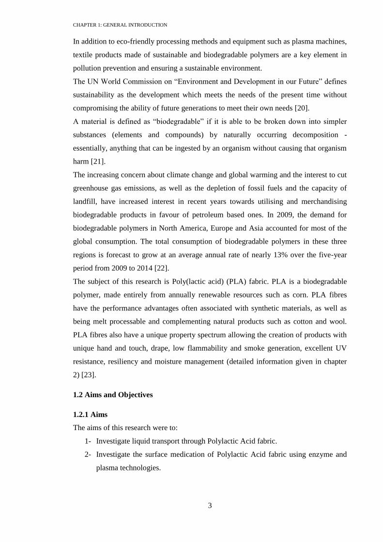
The aims of this research were to:
1- Investigate liquid transport through Polylactic Acid fabric.
2- Investigate the surface medication of Polylactic Acid fabric using enzyme and
plasma technologies.

CHAPTER 1: GENERAL INTRODUCTION
4
1.2.2 Objectives
1- Evaluating the spreading behaviour of textile materials.
2- Establish a numerical model for predicting the vertical wicking rate, spreading
rate and roundness of the drop area for liquid movement through PLA knitted
fabric.
3- Investigate of the influences of plasma and enzyme preparation process on PLA
water transport behaviour, and examine the physical and chemical modification
using Scanning Electron Microscopy (SEM) and X-ray Photoelectron
Microscopy (XPS) respectively.
4- Identify the relationship between determinant parameters of plasma preparation
and the rate of liquid movement through PLA fabric.
5- Identify the relationship between determinant parameters of enzyme preparation
and the rates of liquid movement through PLA fabric.
6- Implement image analysis techniques for textile testing for more accurate and
faster measurements of spreading and wicking rates, as well using the statistical
methods to analyse the data and develop models to predict the textile behaviour.
1.3 Thesis Outline
Chapter 2
This chapter gives a review of PLA fabric, including the manufacture of PLA physical
and chemical properties and potential uses of PLA.
Chapter 3
This chapter provides a literature review of plasma and enzyme technologies and their
concepts and systems, as well the possible applications for textile industry.
Chapter 4
This chapter is divided into two sections:
Section 1: a general literature review of the wetting and wicking properties of
textile materials.
Section 2: an in-depth review of the mathematical background of the wicking
and spreading processes.
Chapter 5
This gives a detailed account of the equipment and methodology used in this research.
Presenting the experimental technique of wicking and spreading, incorporating
image analysis.
The plasma units which were used in this research

CHAPTER 1: GENERAL INTRODUCTION
5
An introduction to experimental design
Chapter 6
Characterisation of PLA knitted fabric, the main substrate used in this research, is
presented in this chapter.
Chapter 7
This chapter deals with the oxygen plasma preparation process of PLA and Polyester
(PET) fabrics, using the Europlasma machine CD400 and the further tests and analyses.
It includes the following:
Spreading tests on PLA and PET
SEM examination of substrates
XPS analysis of the chemical composition of the fabric surfaces
Chapter 8
This chapter involves the study of oxygen plasma preparation of PLA fabric using the
Nanotech PE250 plasma machine. The following techniques were used to assess the
effect of the preparation process on the fabric:
Wicking and spreading tests on PLA
XPS spectra
SEM micrographs
Data analysis using statistical methods
Chapter 9
Enzymatic preparation of PLA fabric using lipase is explained. The following tests and
analyses are included:
Wicking test of PLA fabric
SEM images
XPS spectra
Dyeing
Analysis of the results by statistical methods
Chapter 10
This chapter concludes the thesis by giving:
A comparison between three previously mentioned preparation process in terms
of their effects on PLA fabric
Conclusions
Recommendations for further work
Appendix

CHAPTER 2: LITERATURE REVIEW OF POLYLACTIC ACID FABRIC
6
Chapter 2
LITERATURE REVIEW OF POLYLACTIC ACID FABRIC
Chapter Overview
This chapter explores PLA polymer production, processing and key performance
features as well as the potential textile applications. It outlines the various research
concerned with PLA development.
2.1 Introduction
Poly(lactic acid) is a biodegradable, aliphatic polyester made from lactic acid, which is
usually derived from fermentation of 100% renewable resources such as corn and sugar
beets [24]. The historical development of PLA dates back to 1845 when it was
synthesised by Theophile-Jules Pelouze through the condensation of lactic acid [25].
Poly(lactic acid) was first reported by Carothers in 1932 [26]. This invention was
patented by DuPont in 1954. Since then it was limited mainly to biomedical applications
because of its high manufacturing cost. Since 1990, there have been advances in the
fermentation of glucose, which turns the glucose into lactic acid. This had a dramatic
effect on lowering the cost of producing lactic acid and significantly increased interest
in wide commercial applications of the polymer [27]. In the late 1990 two companies,
Cargill Inc and Dow Chemical, collaborated to produce PLA resin on commercial scale
under the trade name NatureWorksTM
. Currently NatureWorksTM
is wholly owned by
Cargill Inc.
Poly(lactic acid) has the potential to be processed into the types of products where
thermoplastic materials can be employed. Biodegradability makes it a promising
material for many disposable products, such as baby nappies, plastic bags, and films.
PLA is melt-spinnable and has very good fibre- and film-forming properties. Also it can
be used for medical applications, for example in bone fracture fixation, in drug delivery
systems, surgical sutures because it degrades inside human body [28].
Commercially PLA fabric is known as Ingeo “ingredient of the earth”. This was
introduced by NatureWorks TM
. It is being used as alternative name for PLA fabric in
many publications and research works.

CHAPTER 2: LITERATURE REVIEW OF POLYLACTIC ACID FABRIC
7
2.2 Chemistry and production of Poly(lactic acid)
Polylactic acid is derived from lactic acid, which has the chemical formula
HOCH3CHCOOH. Lactic acid is a chiral molecule (chiral molecules exists as ‘mirror
images’ or stereoisomers) [29]. It exists in the two configurations shown in Figure 2.1,
L-lactic acid, and D-lactic acid. The key difference between L-lactic acid and D-lactic
acid is orientation of the methyl group CH3 in relation to and carbonyl group C=O.
Figure 2.1. The two forms of lactic acid [29]
Lactic acid can be synthesised from both non-renewable fossil and renewable feed stock
resources [30, 31]. Production from a renewable resource starts by the photosynthesis
process which produces the carbohydrate sources as illustrated in Figure 2.2, such as
glucose and starch [32]. Generally the lactic acid manufacturing process consists of two
stages: fermentation and purification of the lactic acid. In the fermentation stage, the
starch is converted into dextrose via enzymatic hydrolysis, and then the lactic purified
as shown in Figure 2.2.

CHAPTER 2: LITERATURE REVIEW OF POLYLACTIC ACID FABRIC
8
Figure 2.2. Lactic acid synthesis from renewable resource [32]
The formation of Poly(lactic acid) involves the processing and polymerisation of lactic
acid monomer. Polymerisation of lactic acid can be achieved by condensation
polymerisation and ring opening polymerisation through lactide intermediate.
The condensation polymerisation involves the removal of water by condensation and
the use of solvent under high vacuum and temperature. The disadvantage of this method
is that only low to intermediate molecular weight polymers can be produced, mainly
because of the presence of water and impurities.
The ring opening polymerisation method is used by Cargill Dow (the polymer provider
for this research). The process is illustrated in Figure 2.3. In the first step the water is
removed to produce a low molecular weight pre-polymer. This pre-polymer is then
depolymerised to form a cyclic intermediate dimer known as lactide which is then
purified to polymer grade using distillation. Finally the purified lactide is polymerised
into polylactide pellets [33].

CHAPTER 2: LITERATURE REVIEW OF POLYLACTIC ACID FABRIC
9
Figure 2.3. PLA manufacturing process [32]
Production of the cyclic lactide dimer results in three potential forms, pure D-lactide
and L-lactide which is usually known as meso lactide, and mixture of D and L-lactide
which is known as racemic dimer. PLLA poly(L-lactic acid) is more crystalline, and
degrades more slowly than PDLA poly(D-lactic acid) [34].
The ratio of L- to D-lactic acid units, which can be controlled during polymerisation,
strongly influences the physical properties of polymer, resulting in a broad spectrum of
properties. For example, a L:D-lactide monomer ratio lower than 78:22 will result in an
amorphous polymer, whereas a higher ratio gives a semi-crystalline material [35, 36].
Fully amorphous materials can be made by including a relatively high D content
(greater than 20%), while highly crystalline materials are obtained when D content is
low (less than 2%) [37].
2.3 Sustainability, Degradability and Recycling of PLA
The current use of fossil-based polymers is unsustainable. Polymer materials such as
polyethylene, polystyrene and polypropylene, are derived from non-renewable fossil
resources, such as crude oil and natural gas. The majority of the polymers are landfilled
at the end of their useful life. This creates large amounts of non-biodegradable solid
waste, and causes a loss of valuable non-renewable resource. In addition polymer
additives such as plasticisers, thermal stabilisers and flame retardants, colorants can
cause environmental hazard due to possible leaching into the soil and underground
water [38].

CHAPTER 2: LITERATURE REVIEW OF POLYLACTIC ACID FABRIC
10
Recycling and reuse of traditional polymer materials are limited. Although there is a
considerable effort to increase the polymer recycling rates, the potential for recycling is
limited by a number of economic, environmental and social factors. These include the
difficulties in collecting and separating the waste plastics from the end-user, the costs of
building and operating the recycling facilities and potential environmental impacts from
the recycling.
PLA is biodegradable, renewable and environmentally sustainable in its production and
use. It can itself be constantly renewed without degradation in quality or performance
and has a minimum environmental impact. It provides alternative environmentally
friendly, equivalent functions, and is cost competitive with traditional polymers. The
following is brief introduction into PLA sustainability, degradability and recycling.
2.3.1 PLA Sustainability
All materials and resources which can be replenished at a rate that is equal to, or
sometimes greater than their rate of consumption can be termed as sustainable materials.
This can be done either through a natural process, or at times through human-engineered
ways. Sustainable resources can also be considered as materials whose use will not
deplete the main supply, such as in the case of solar and wind energy.
Environmental sustainability is about making products that serve useful market and
social functions, with lower detrimental environmental impact than the currently
available alternatives [39]. During polymer processing three measures are used to assess
the impact on the environment: fossil energy use; greenhouse gas emissions; and water
use [31].
According to data published in 2003 [40], the first generation of PLA production
systems were estimated to use 25 to 55% less fossil energy than the petroleum-based
polymers. Process development towards using wind-based renewable energy helped to
reduce further the use of fossil energy. In a report published in June 2007 [41],
Natureworks LLC revealed the new eco-profile of PLA corn-to-pellet polymer process.
It showed approximately 50 percent less fossil fuel use in comparison to the previous
data in 2003.
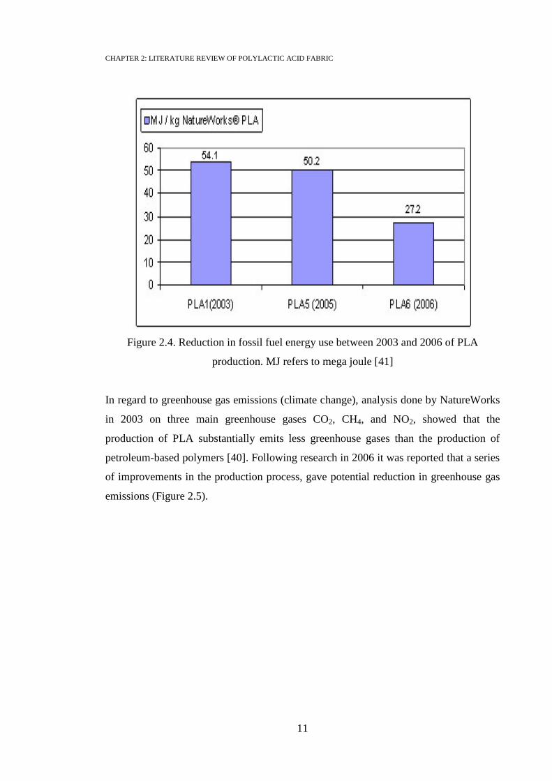
CHAPTER 2: LITERATURE REVIEW OF POLYLACTIC ACID FABRIC
11
Figure 2.4. Reduction in fossil fuel energy use between 2003 and 2006 of PLA
production. MJ refers to mega joule [41]
In regard to greenhouse gas emissions (climate change), analysis done by NatureWorks
in 2003 on three main greenhouse gases CO2, CH4, and NO2, showed that the
production of PLA substantially emits less greenhouse gases than the production of
petroleum-based polymers [40]. Following research in 2006 it was reported that a series
of improvements in the production process, gave potential reduction in greenhouse gas
emissions (Figure 2.5).

CHAPTER 2: LITERATURE REVIEW OF POLYLACTIC ACID FABRIC
12
Figure 2.5. Greenhouse gas emissions from cradle to factory gate for PLA production.
All emissions values were converted to CO2 equivalents [41]
The third parameter for measuring the effect of polymer production on the environment
is the water use. Figure 2.6 compares the gross water use of traditional polymers and
PLA. The gross water use is the sum of public supply, river, canal, sea and well water
used as cooling water, process water and irrigation water. Despite the use of irrigation
water during corn growing and the two water-based processes (dextrose and lactic acid
production) the total amount of water required is competitive with the best performing
petrochemical polymers.

CHAPTER 2: LITERATURE REVIEW OF POLYLACTIC ACID FABRIC
13
■ Process water Cooling water □ Irrigation water
Figure 2.6. Water consumption during polymer production
PLA (B/WP) refer to PLA produced using biomass and wind power [40]
2.3.2 PLA Biodegradability
PLA degrades under various modes, such as hydrolytic degradation, thermal
degradation, photo degradation, and biodegradation [42]. Generally speaking,
biodegradation is caused by naturally occurring microorganisms such as bacteria and
fungi, while the other degradation modes are predetermined by standard test conditions.
The term "biodegradability" was initially defined as the ability of materials to be easily
degraded with microbes at 20-25°C to release carbon dioxide and water in the natural
environment. PLA is stable under typical end-use and storage conditions at ambient
temperature. It degrades when it is exposed to high temperature (>60°C) and high-
humidity (>80% RH) conditions, such as in a composting environment.
PLA was reported to take years to degrade in ambient [43, 44]. It degrades quickly
when composted under certain temperature and humidity and availability of bacteria
(Figure 2.7). So in terms of compostability in compliance with ISO standards, PLA is
now considered a biodegradable plastic [42].
Kg w
ater
/ K
g p
oly
mer
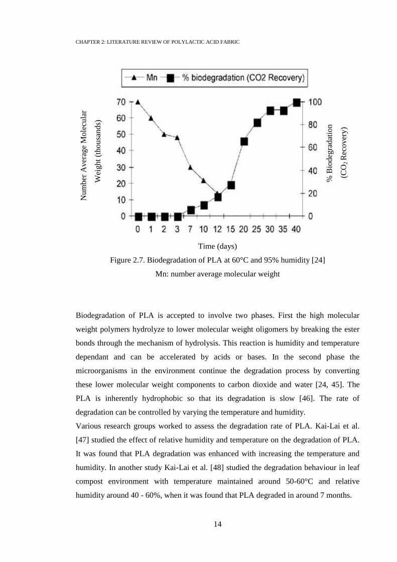
CHAPTER 2: LITERATURE REVIEW OF POLYLACTIC ACID FABRIC
14
Time (days)
Figure 2.7. Biodegradation of PLA at 60°C and 95% humidity [24]
Mn: number average molecular weight
Biodegradation of PLA is accepted to involve two phases. First the high molecular
weight polymers hydrolyze to lower molecular weight oligomers by breaking the ester
bonds through the mechanism of hydrolysis. This reaction is humidity and temperature
dependant and can be accelerated by acids or bases. In the second phase the
microorganisms in the environment continue the degradation process by converting
these lower molecular weight components to carbon dioxide and water [24, 45]. The
PLA is inherently hydrophobic so that its degradation is slow [46]. The rate of
degradation can be controlled by varying the temperature and humidity.
Various research groups worked to assess the degradation rate of PLA. Kai-Lai et al.
[47] studied the effect of relative humidity and temperature on the degradation of PLA.
It was found that PLA degradation was enhanced with increasing the temperature and
humidity. In another study Kai-Lai et al. [48] studied the degradation behaviour in leaf
compost environment with temperature maintained around 50-60°C and relative
humidity around 40 - 60%, when it was found that PLA degraded in around 7 months.
Num
ber
Aver
age
Mole
cula
r
W
eight
(thousa
nds)
% B
iodeg
radat
ion
(C
O2
Rec
over
y)

CHAPTER 2: LITERATURE REVIEW OF POLYLACTIC ACID FABRIC
15
A study by Lunt [49] found that PLA takes 123 months to start to biodegrade in a
solution of water at 4°C, and 3.5 days at 70°C. Whereas at 60°C under composting
conditions PLA takes 45 days to fully decompose.
Another study [50] showed the percentage decrease in the tensile strength and relative
viscosity of the PLA fibres following soil burial as a function of time. The results are
illustrated in Figure 2.8 indicating that degradation proceeds slowly, but steadily. After
2 years, the fibres have lost about 50% of their initial strength.
Time (years)
Figure 2.8. Changes in the tenacity and the relative viscosity of PLA multifilament
(50d/24f) in soil burial test [50].
An investigation of the degradation behaviour of PLA fibre [50], found that PLA fibres
subjected to 18 months of soil burial showed that a number of fine cracks appeared
perpendicular to the fibre axis. It was supposed that the hydrolytic degradation occurs
preferably in the amorphous regions, which are sandwiched between two crystalline
zones of the so-called "shish-kebab" structure.
The slow degradation process and degradation mechanism of PLA is considered unique
and differs from many other biodegradable polymers that degrade by a single-step
Rel
ativ
e vis
cosi
ty
Ten
sile
str
ength
ret
ain
ed (
%)

CHAPTER 2: LITERATURE REVIEW OF POLYLACTIC ACID FABRIC
16
surface erosion process. This is a beneficial feature in applications such as apparel and
geotextile as it takes relatively long time to degrade.
2.3.3 PLA Recycling
The PLA polymer is formed from reversible polycondensation reactions and can be
depolymerised by hydrolysis. This equilibrium results in the recycling ability for PLA
[51]. Manufacturing waste or post-consumer PLA materials can be recycled by
chemical means to produce lactic acid monomers or oligomers. These materials can be
fed to the front end of a manufacturing process for making PLA lactide. The recycling
can be carried out with water at a wide range of temperatures (100-250°C). The reactor
times for PLA hydrolysis are in the order of hours, and depend on reactor temperature
and catalyst level.
2.4 Polylactic Acid Fibre Properties
PLA is expected to play a big role as a viable, biodegradable replacement because of its
physical polymeric properties that lie somewhere between those of polypropylene (PP)
and polyethylene terephthalate (PET). It was reported that the rigidity and clarity of
PLA is similar to Polystyrene (PS) or Poly(ethylene terephthalate) (PET) [42].
Because PLA is polyester, it might be expected to behave similarly to polyester (PET).
Indeed, both polymers need to be dried before melting to avoid hydrolysis, both
polymers form fibres via melt extrusion, and fibres from both polymers can be drawn to
develop useful tensile strength. However there are differences, arising from PLA’s
renewable source as opposed to PET’s mineral source, and the polymer structures. With
regard to polymer structure, PET is aromatic polyester, incorporating a benzene ring in
each repeat unit while PLA is an aliphatic polyester with pendant methyl groups, as
shown in Figure 2.9. In addition to this PET is nominally linear, while the PLA
molecule tends to assume a helical structure. The following paragraphs present the PLA
properties and point out the main difference from other polymers.

CHAPTER 2: LITERATURE REVIEW OF POLYLACTIC ACID FABRIC
17
Figure 2.9. The chemical structures of PET and PLA
2.4.1 Thermal Properties
The thermal characteristics of the PLA are important criteria in many applications. PLA
is a stiff polymer at room temperature. Table 2.1 shows a comparison of Tg and Tm of
PLA and synthetic polymers [52]. The low melting point of PLA in comparison to PET
is considered the main obstacle for PLA to replace PET in the market and hinders its
development for a wider range of applications. However, the properties of PLA can be
modified by adjusting the ratio and the distribution of the D- and L- isomers in the
polymer chain, and melting points as low as 130ºC and as high as 220ºC have been
obtained [53].
Table 2.1. Comparison of Tg, Tm of PLA and other synthetic polymers [52]
Fibre Glass transition temperature Melting temperature
PLA 60-65 172-178
PET 70-80 265
Nylon 6.6 (dry) 60-70 265
PP -5 160-165
2.4.2 Mechanical Properties
Mechanical properties are affected by molecular weight, orientation of molecular
chains and crystallinity that develops during drawing. The tenacity at break (32–36 cN

CHAPTER 2: LITERATURE REVIEW OF POLYLACTIC ACID FABRIC
18
tex–1
) is higher than for natural fibres although, of course, it can be varied according to
the degree of drawing during fibre processing.
The tensile properties of PLA fibre as used in staple form for textile processing are
shown in Figure 2.10. Clearly they are very different from those of high tenacity
polyester and more akin to wool with a high fibre extension when stressed and
relatively low final tenacity. The initial modulus (at 2% extension) is very similar to
many other textile fibres, but the yield point is very marked, the fibres (and spun yarns)
stretching very easily once past this point.
Extension (%)
Figure 2.10. Tenacity- Extension curve for PLA and other common textile fibres
(20ºC, 65%) [53]
2.4.3 Hydrophilicity of PLA
Studies on the moisture management of PLA such as wear comfort, sorption, wetting,
wicking, contact angle, have not been reported widely in the literature, especially
regarding the PLA fabric.
Water is a polar molecule because of a slightly negative charge on the oxygen atom and
slightly positive charges in the two hydrogen atoms. Water molecules bond easily with
molecules with an opposite charge that come nearby, such as polymer with carboxyl,
Ten
acit
y (
cN t
ex-1
)

CHAPTER 2: LITERATURE REVIEW OF POLYLACTIC ACID FABRIC
19
hydroxyl, or amine functionalities. Water penetrates the fibres through their pores and
capillaries, and is bound by polar groups on the polymeric chain. Cellulosic fibre
structures such as cotton have negatively charged groups due to ionised hydroxyl groups
which attract water molecules and make them highly water absorbent and relatively
poor in wicking. On the other hand, synthetic fibres such as PET and PLA have
hydrophobic chemical groups, therefore tend to wick the water but not absorb it. PET
polymer is considered hydrophobic (Table 2.3) in comparison with natural protein and
cellulosic fibres. This mainly due to the existence of the benzene rings in terephthalic
acid and the -CH2-CH2- groups in ethylene glycol. However, the ester groups confer
some degree of polarity on the molecules, so that the fibres are not as hydrophobic as
hydrocarbon fibres such as polyethylene and polypropylene.
Generally polymers containing a large number of C-H bonds such as PLA are known to
be hydrophobic [54]. Dugan [55] reported that in PLA water molecules have access to
the polar oxygen linkages in the PLA, therefore it has higher hydrophilic nature than
other thermoplastic materials such as PET, nylon, and polypropylene. Dugan also
suggested the possibility of using PLA for making the 4DG fiber, which is considered
the most effective moisture transport fibre cross-sectional shape because of its grooves
(Figure 2.11) and hydrophilic finish.
Figure 2.11. 4DG fibre [55]
In another review of PLA, Blackburn [53] said “PLA shows excellent wicking ability.
This property and the additional properties of fast water spreading and rapid drying
capability give the fibre a very positive inherent moisture management characteristic”.

CHAPTER 2: LITERATURE REVIEW OF POLYLACTIC ACID FABRIC
20
In regard to wicking and contact angle the only quantitative information has been
reported by Patrick [56], shown in Table 2.2, but no clear explanation was given about
the testing conditions. Also a comparison of moisture regain of PLA with other fibres
shown in Table 2.3.
Table 2.2. Wicking rate and contact angle of PLA and PET [57]
L-W refers to Lucas-Washburn equation, PET: Poly(ethylene terephthalate)
property PET PLA
Wicking (L-W slope;
higher slope, more wicking 0.7-0.8 (no finish)
6.3-7.5 (no finish)
19-26 (with finish)
Contact angle 82 76
Table 2.3. Moisture regain % of fibres at standard conditions
(21°C, 65% r.h) [57]
Fibre types Moisture Regain
PLA 0.4-0.6
PET 0.2-0.4
Nylon 6 4.1
Viscose rayon 11
Cotton 7.5
Silk 10
Wool 14-18
2.4.4 Flam ability properties
PLA fibre shows improved self-extinguishing characteristics when compared with PET
or nylon fibres. It burns for only two minutes with low smoke generation (63m2/kg)
after the flame is extinguished, while PET burns for 6 minutes with higher smoke
generation (394m2/kg). Table 2.4 shows a comparison of PLA and PET flame
properties. The larger LOI (Limiting Oxygen Index) compared to most other fibres,
indicates that PLA has better flame retardant characteristics. PLA releases significantly
less visible smoke than PET, so visibility hazards in a fire are reduced. PLA’s burning
properties make it attractive for use in upholstery, carpets, and fabrics for cars.

CHAPTER 2: LITERATURE REVIEW OF POLYLACTIC ACID FABRIC
21
Table 2.4. Flame properties of PLA and PET [53]
2.5 Scouring, Bleaching and Dyeing of PLA Fabric
PLA is a linear aliphatic polymer; its resistance to hydrolysis is relatively poor. The
degree of hydrolysis is influenced by pH and temperature of surrounding media as well
as the treatment time. Attention should be made to sensitivity of PLA to the surrounding
parameters because it could cause reduction in the molecular weight of the polymer and
the strength of a yarn or fabric.
Hydrolytic degradation of PLA-based materials involves the cleavage of ester groups.
Therefore the reaction could be catalyzed by the presence of hydronium and hydroxide
ions. The high concentration of hydroxide ions in alkaline media strongly accelerates
the hydrolytic degradation of PLA-based materials. Similar to alkaline media, acidic
media accelerate the hydrolytic degradation of PLA-based materials [58].
Various preparation and dyeing processes of PLA and their influences on the fabric
properties were studied by Jantip [59]. The following section provides description of the
wet processing procedures of PLA and their effects on its properties.
2.5.1 Scouring and Bleaching
The purpose of scouring is to remove spin finish and wax. Scouring generally involves
the use of hot alkaline solution, which is normally caustic soda solution with detergent.
Most of the impurities are removed by being converted into soluble substances that can
be washed away with water.
Jantip [59] used solution of 2 g/l soda ash and 0.5 g/l Kieralon Jet B conc. (non-ionic
surfactant, BASF) at 60°C for 20 minutes. After scouring, the fabric was rinsed with
cold water and subsequently dried at room temperature. It was found this scouring
procedure did not have deleterious effect on the properties of PLA.
Fibre PLA PET
Flammability
Continues to burn for
two minutes after flame
removed
Continues to burn for six
minutes after flame is
removed
Smoke generation 63 m2.kg
-1 394 m
2.kg
-1
LOI 26% 22%

CHAPTER 2: LITERATURE REVIEW OF POLYLACTIC ACID FABRIC
22
In the same study a bleaching process in strong alkaline solution was reported. The
solution was made of 6 ml of 50% (w/w) caustic soda, 5 ml/l of 35% (w/w) hydrogen
peroxide and 0.5 g/l Baystabil DB (stabiliser, BASF) at 95°C for 30 minutes. The fabric
was then rinsed in hot water (60°C) and cold running water respectively. The effect of
this process was a 20% weight loss, and the Ingeo fibre becoming thinner. The tenacity
and the initial modulus of yarn were lowered substantially. This could be related to the
surface erosion by the alkaline solution [60, 61]. However the reduction in molecular
weight was insignificant.
2.5.2 Dyeing
The dyeing process is important because the various methods and subsequent finishing
treatments may have significant chemical and physical effects. PLA can be dyed using
disperse dyes. According to DyStar recommendations, the optimum dyeing conditions
for PLA are 110°C for 30 minutes at pH5. Practical experience has shown that the use
of higher temperatures or longer times of dyeing can cause degradation of the polymer.
The refractive index of PLA is lower than that of PET or nylon, so it can achieve higher
colour yield [55, 62]. The colour yields can be increased by altering the proportions of
the D- and L-isomers in the fibre, and thereby changing the amorphous/crystalline
ratios. Higher D-levels have more amorphous and less crystalline regions [63]. Fibres
with higher D-isomers display greater colour strength with respect to low D-fabrics in
all dyes and all concentrations, as a result of the greater number of amorphous regions
in high D-fibres with respect to low D-fibres.
In the application of a dye mixture to produce a black shade, high D-fibres are able to be
dyed to an excellent black shade, whereas low D-fibres appear very brown, due to less
exhaustion of the blue component of the mix.
In terms of wash fastness, there is very little difference between high D-fibres and low
D-fibres; this is because the glass transition temperature for both fibres is very similar.
The colour fastness of PLA tends to be slightly worse than for PET. One reason for
lower wet fastness is believed to be due to more movement of dye to the surface by
thermo-migration, during post-heat treatments. It may also be that a lower thermosetting
temperature is used for PLA (130°C) compared to PET (190°C).

CHAPTER 2: LITERATURE REVIEW OF POLYLACTIC ACID FABRIC
23
The dyeing of PLA/wool blends does not present a problem as both fibres have the
same characteristic with regard to alkali sensitivity, and with similar stress-strain
profiles, there would seem to be some benefits compared to PET/wool.
2.6 Applications of Polylactic Acid
Polylactic acid offers unique features of biodegradability, thermoplastic processibility
and ecofriendliness that offer potential for wide range of applications such as apparel,
furnishings, binder fibres, wipes, hygiene, packaging, agricultural. The following
sections discuss the possible potential applications of PLA.
2.6.1 Apparel
Currently PLA fabrics are being used for various kinds of garment such as t-shirts,
underwear, casual wear, sportswear, jeans/denim and jackets. The key performance
features of PLA in apparel sector are the following:
PLA can be produced as both filament and spun yarns. Fabric produced from
spun yarn has natural hand and are considered to feel similar to cotton in this
respect. Fabrics from filament yarns have a cool and soft hand and exhibit a high
fluidity or drape with a degree of elasticity [53].
The comfort of textile materials is a very important issue for personal well-being
and the quality of life; it is mostly related to the transfer of heat and water
vapour through textile structure. Moisture management of good wicking, faster
spreading and drying provide garments with comfort characteristic. The superior
moisture regaining and wicking properties over those of PET, as explained in
Section (2.1.5.3), give considerable interest in using PLA either as an inner
wicking layer or as blend with other natural fibres. The comfort test applied by
the Hohenstein Institute [64] concluded that the wearers of the Ingeo
fibres/cotton or fabric consisting of 100% Ingeo fibres will perceive
significantly improved physiological comfort versus fabric made of PET/cotton
or the 100% DP (durable press) resin treated cotton fabrics, as shown in Figure
2.12.

CHAPTER 2: LITERATURE REVIEW OF POLYLACTIC ACID FABRIC
24
Figure 2.12. Total comfort test, DP: durable press [64]
PLA fibres have an inherent ability to hold a crease or fold. This excellent crease
retention property facilitates pleats or wrinkles processing of PLA fabrics [65].
High resiliency and lower specific gravity than natural fibres can give PLA
fabrics a light and lofty feel. These properties have been used to provide an
effective wadded layer, e.g. ski jacket.
However with these positive features of PLA there are restrictive technical issues
because of relatively low melting temperature and hydrolysis under high temperature
and alkaline conditions. The required dyeing technology at lower temperature (105-
110°C) with good colour fastness and the need to limit ironing to around l20°C have
hampered the use of PLA in some apparel applications, for instance when it is mixed
with other fibres.
2.6.2 Industrial Fabrics
Woven and nonwoven fabrics made from PLA fibres are being considered for
automobile manufacturing, in applications such as floor mats, seat fabric, seat cushions,
ceiling fabric, and partition boards. Toyota has already employed a new type of spare-
tyre box cover using Kenaf/PLA board, which is manufactured by heat compression
moulding of a Kenaf/PLA (weight-based blend ratio: 7/3) fibre web [65].
Other uses of PLA fabrics have been reported including woven fabrics; mesh fabrics,
knitted fabrics, spunbond fabrics, and nonwoven fabric for industrial uses such as signs,

CHAPTER 2: LITERATURE REVIEW OF POLYLACTIC ACID FABRIC
25
awnings, ground covers, headrest covers, vehicle seat textiles, and tarpaulins. Headrest
covers made from PLA spunbond fabric were introduced in JR trains in Japan.
2.6.3 Filters
PLA polymer is being used for filter products for industry such as automotive and
chemical industries, and food applications. PLA has been proved by FCN (Food
Contact Notification) to be safe for food contact. PLA filters have been used as filters
for coffee, tea and juice. Presumably PLA has been used for air conditioning filters as
an antibacterial/ antifungal material which provides benefit for management of sanitary
wastes [65].
2.6.4 Towels and Wipes
The comfort, fast drying and low shrinkage properties of PLA outperformed cotton, and
it has been successfully used for making towels either as 100% PLA or in blends with
cotton. Towels made of PLA do not generate bad smells even after long time use. This
can be related to the antibacterial/antifungal property of PLA.
Another potential application for PLA is for nonwoven wipes such baby nappies,
feminine hygiene and facial tissues. Again the superiority of PLA’s wicking property in
comparison with other synthetic polymers which comprise around 50% of wipes
industry, has led to considerable interest for use of PLA in wipe sector.
2.7 Polylactic Acid Drawbacks
The following issues are considered to be disadvantages of PLA:
Slow degradation rate: PLA degradation rate depends on the crystallinity,
molecular weight, molecular weight distribution, morphology, water diffusion
rate into the polymer, and the stereo isomeric content [66]. The slow degradation
rate in vivo cannot meet the different requirements of various medical
applications such as tissue engineering scaffolds, sutures, and drug delivery
systems. Also, for PLA products such as cloth or bottles at the end life cycle,
degradation normally takes long time, this creates problem in landfill.
Hydrophobicity: PLA is relatively hydrophobic, though it is more hydrophilic
than PET. For instance this results in low adhesion onto the surface and poor cell
affinity in medical applications.

CHAPTER 2: LITERATURE REVIEW OF POLYLACTIC ACID FABRIC
26
Lack of reactive side-chain groups: PLA is chemically inert with no reactive
side-chain groups, making its surface and bulk modifications a challenging task.
Poor toughness: One of the major shortcomings of PLA is its brittleness, with
less than 10% elongation at break [67]. The poor toughness gives poor impact
resistance and limits its use in applications that need plastic deformation at
higher stress levels (e.g., screws and fracture fixation plates) [22]).
Recycling and composting: because of the different origin of PLA from other
plastics, the householder must separate the PLA from other plastic materials and
put them in special composting bins different from the normal recycling ones. In
addition to this, a compost infrastructure and facilities are required.
Another issue of PLA polymer production is it is made from food resources such
as corn, with the world already facing troubles in food prices and starvation.
Another downside of PLA is that it is being made typically from genetically
modified corn, at least in the United States. It was reported the feedstock used
by Cargill-Dow for PLA manufacture is genetically modified (GM) corn (has a
higher than normal starch content) [68]. This genetic modification could have
serious effects on environment and human health in the future.

CHAPTER 3: INTRODUCTION TO LOW TEMPERATURE PLASMA AND ENZYME TECHNOLOGIES- THEORY AND
APPLICATION
27
Chapter 3
INTRODUCTION TO LOW TEMPERATURE PLASMA AND ENZYME
TECHNOLOGIES - THEORY AND APPLICATION
Chapter Overview
This chapter provides a general review of plasma and enzyme technologies and their
applications in surface modifications of textile materials. The chapter is divided into
two sections. First section concerns plasma concepts and the possible applications for
textile industry and reviews the up-to-date research about plasma treatment of
Poly(lactic acid) fibres. The second section introduces enzyme technology and its usage
for textile processing, in particular with regard to Poly(lactic acid) fibres.
3.1 Plasma Technology
3.1.1 Introduction
The textile industry is always in search of new technologies that lower costs, increase
productivity, and decrease waste. Plasma treatment of textile materials is considered a
possibility for replacing or enhancing many current wet chemical processes.
The concept of plasma dates back to Langmuir (1928) [69]. Plasma is an ionised gas -
also considered the fourth state of matter - containing electrons, ions, and neutral
particles (atoms, molecules) [70]. The positively and negatively charged species present
in approximately the same amount; therefore the plasma is known as quasi-neutral.
Plasma is classified into hot-temperature and low-temperature plasma [71]. Hot-
temperature plasma includes solar coronas and nuclear fusion generated by
thermonuclear reaction, their temperature is about 100 million degrees.
Low-temperature plasmas (cold plasma) are commonly used in material processing,
described as non-equilibrium and non-thermal. It is considered non-equilibrium because
the charged species have a much higher kinetic energy than neutral species. The non-
thermal property of low-temperature plasma arises from the fact that although the
electron temperature is several tens of thousands of Kelvins [72], because of the low
density and low heat capacity of the electrons, the very high temperature of electrons
does not make the plasma hot and the gas temperature remains at 100 K.

CHAPTER 3: INTRODUCTION TO LOW TEMPERATURE PLASMA AND ENZYME TECHNOLOGIES- THEORY AND
APPLICATION
28
Low-temperature plasma can be subdivided according to the gas pressure, to low-
pressure plasma and atmospheric pressure plasma. The following review mainly
concerns low pressure plasma as this plasma was used for the experiments of this
research, and it will be termed thereafter as low-pressure cold plasma.
3.1.2 Design and Generation of Low-Pressure Cold Plasma System
To reach the plasma state, energy for the ionisation must be input into the gas atoms
from an external source [73]. Electrons and ions are produced in the gas phase when
electrons or photons with sufficient energy collide with the neutral atoms and molecules
in the feed gas. Low-pressure cold plasma technology is also referred to as vacuum
plasma. Three essential items must be provided to generate low pressure cold plasma:
(1) an energy source for the ionisation, (2) a vacuum system for maintaining a plasma
state, and (3) a reaction chamber [74, 75]. Schematic representation of low-pressure
cold plasma system with RF generator is shown in Figure 3.1. The reaction chamber
contains a pair of electrodes and a substrate stage.
Generally, the electric energy for ionisation is used as the energy source because of
convenience of handling. Alternating current (AC) can be used, with various frequency
such as low frequency (10-20 KHz), radio frequency (13.56 MHz), and microwave
frequency (2.45 GHz). The electric power is basically supplied to gas atoms in the
reaction chamber in a capacitive coupling manner with the electric generators [76].
The plasma generation consists of three steps. First the vacuum chamber is pumped
down to a pressure, known as base pressure, in the range of 10-2
to 10-3
mbar with the
use of high vacuum pumps; this step ensures stable and pure gas plasma treatment.
Secondly, the gas is introduced in the vessel, until reaching the required working
pressure, usually around 0.1 to 10 mbar, then the generator is switched on and the
process gas is ionised.
The configuration of a plasma system can differ widely depending on the purpose of
usage as shown in Figure 3.2; the size of plasma chamber can be adjusted according to
the size of products to be treated.

CHAPTER 3: INTRODUCTION TO LOW TEMPERATURE PLASMA AND ENZYME TECHNOLOGIES- THEORY AND
APPLICATION
29
Figure 3.1. Schematic representation of low-pressure cold plasma system [75]
Figure 3.2. Illustration of plasma systems for different usages [75]

CHAPTER 3: INTRODUCTION TO LOW TEMPERATURE PLASMA AND ENZYME TECHNOLOGIES- THEORY AND
APPLICATION
30
3.1.3 Interaction between Plasma and Polymeric Materials
Plasma is used to supply the input energy required to initiate chemical and physical
reactions at the polymer surface. As the plasma is a mixture of charged ions, molecules,
atoms, various reactions occur simultaneously in the plasma system. The interaction of
plasma with a substrate can be divided into plasma treatment (non-polymer forming
plasma) and a plasma polymerisation (polymer-forming plasma) [77]. The reactions
initiated by plasma depend mainly on the nature of plasma gases, as well as the energy
level of the plasma and nature of polymeric materials [78]. If the plasma gas has high
proportions of hydrogen and carbon atoms in its composition, such as methane, ethylene
and ethanol, the plasma will result in plasma polymerisation which leads to deposition
of polymer materials.
The plasma treatment occurs when using gases such as argon, helium, nitrogen and
oxygen, and leads to changes in surface properties of a substrate. The following gives
the main mechanisms of the plasma treatment:
Etching reaction
When polymers are exposed to plasma, weight loss occurs and the topmost layer is
stripped off. Etching of materials by plasma can occur by means of physical sputtering
and chemical etching. Physical sputtering process is a knock-on process by ions with
high kinetic energy.
In sputtering, ions accelerated across the sheath potential bombard a surface with high
energy. The sudden energy impulse can immediately eject surface atoms outward.
Sputtering requires plasma conditions with high-ion energies. These conditions exist in
low pressure, and where mean-free paths are long as well. As a mechanical process,
sputtering lacks selectivity. It is sensitive to the magnitude of bonding forces and
structure of a surface rather than its chemical nature, and quite different materials can
also sputter at similar rates.
In chemical etching, plasma species merely react with a surface according to elementary
chemistry, forming volatile reaction products which are carried away by gas flow.
Implantation reaction
Implantation is a recombination reaction between the radical generated at the polymer
surface and the radical activated from gas molecules. Gas molecules such as oxygen and
nitrogen are activated by plasma; the activated oxygen and nitrogen species interact

CHAPTER 3: INTRODUCTION TO LOW TEMPERATURE PLASMA AND ENZYME TECHNOLOGIES- THEORY AND
APPLICATION
31
with the polymer surfaces, and then, special functional groups such as hydroxyl,
carbonyl, carboxyl, and amino groups are formed at the surface. As a result,
implantation reactions lead to large changes in the surface properties of the polymer, for
example, polyethylene film treated by oxygen plasma showed enhancement in the
hydrophilicity and surface energy increased from 32.9 mN/m into 62.4 mN/m.
3.1.4 Plasma Treatment Conditions
The main conditions that govern the plasma treatment are the nature of the gas used,
flow rate, discharge power, and the duration of the treatment.
3.1.4.1 Nature of Treatment Gas
The result of plasma treatment depends strongly on the nature of the gas. For example
oxygen plasma treatment is oxidising in nature. Oxygen plasma is most commonly
employed to modify polymer surfaces. It is well known that the oxygen plasma can
react with a wide range of polymers to produce a variety of oxygen functional groups,
including C-O, C=O, and O-C-O. In oxygen plasma, two processes occur
simultaneously including (i) etching of the polymer surface through the reaction of
atomic oxygen with the surface carbon atoms, giving volatile reaction products, and (ii)
formation of oxygen functional groups at the polymer surface through the reactions
between the active species obtained from the plasma and surface atoms. The balance of
these two processes depends on the operation parameters [78].
3.1.4.2 Flow Rate and System Pressure
The gas flow rate and system pressure are relatively connected, as the gas flow rate
increases the pressure inside the chamber increases. Basically above a certain level of
discharge power, the gas flow rate determines the number of active species and the
pressure affects the energy per active species because the higher the pressure, the higher
the probability of collision between plasma species which leads to loss of energy of the
species before interacting with the material [79]. For example Figure 3.3 illustrates the
weight loss of Nylon 6 treated by air plasma for 5 minutes with different values of
power. The weight loss increases with the flow rate at every power value in the low-
flow-rate region. As the flow rate was further increased, the weight loss deviated from
linearity and started to decease [80].

CHAPTER 3: INTRODUCTION TO LOW TEMPERATURE PLASMA AND ENZYME TECHNOLOGIES- THEORY AND
APPLICATION
32
Flow rate (cm3/min)
Figure 3.3. Effect of gas flow rate on weight loss of Nylon 6 treated by air plasma
for 5 minutes (○) plasma discharge at 100 W, (●) 70 W, (∆) 50 W, (▲) 30 W [80]
3.1.4.3 Discharge Power
Discharge power is electric energy which is usually released from capacitor to ionise the
gas. The intensity of plasma is a combined factor of pressure and discharge power. The
breakdown energy necessary to produce plasma varies from one gas to another.
Normally, the higher the discharge power applied, the more kinetic energy the plasma
species will carry, resulting in strong intensity of plasma action. In general, there will be
a change in the total amount of the excited particles inside the plasma and their energy
level accordingly when the input power increases under a constant pressure.
3.1.4.4 Duration of the Treatment
The duration of treatment plays an important role in the plasma treatment. Generally
speaking, the longer the duration of treatment, the more severe the modification of the
material surface, as it gives more time for the plasma species to attack the substrate, and
damage the surface, therefore the optimum time that serves the purpose of the treatment
has to be found.
Wei
ght
loss
(%
)
CHAPTER 3: INTRODUCTION TO LOW TEMPERATURE PLASMA AND ENZYME TECHNOLOGIES- THEORY AND
APPLICATION
33
3.1.5 Advantages and Disadvantages of Plasma Technology
The advantages of plasma treatment could be summarised as following:
Modification can be confined to the surface layer without modifying the bulk
properties of the polymer; typically, the depth of modification is less than 1000
Angstrom.
Excited species in plasma can modify the surfaces of all polymers, irrespective
of their structures and chemical reactivity.
By the selection of the feed gas to plasma reactor, it is possible to achieve the
desired type of chemical modification for the polymer surface.
The use of plasma can avoid the problems encountered in wet chemical
treatments such as residual chemical in the effluent and swelling of the substrate.
Modification is fairly uniform over the whole surface.
The disadvantage of plasma treatment can be summarised as following:
The plasma is normally carried out in a vacuum although an atmospheric type is
being developed, thereby increasing the cost of the operation.
The processing parameters are highly system dependant that is the optimal
parameters have to be developed and optimised for one system, and usually
needs to be modified for application to another system.
The scale-up of an experimental set-up to large production reactor is not a
simple process.
The plasma process is so complex that it is difficult to achieve a good
understanding of the interaction between the plasma and the surface necessary
for a good control of the plasma parameters, such as power level, gas flow rate,
gas composition, gas pressure and sample temperature.
It is very difficult to control precisely the amount of a specific functional group
formed on the sample surface.
3.1.6 Plasma Applications for Textiles
Plasma can be used for various textile applications such as desizing, dyeing,
hydrophilicity enhancement; the following is summary of some of the plasma treatment
applications:

CHAPTER 3: INTRODUCTION TO LOW TEMPERATURE PLASMA AND ENZYME TECHNOLOGIES- THEORY AND
APPLICATION
34
3.1.6.1 Plasma De-sizing
During weaving, warp yarns are exposed to considerable mechanical strains. To
enhance the weaving efficiency, warps are coated with a sizing agent to increase the
strength and reduce the hairiness. The sizing agent is most often based on starch or
synthetic sizing agents such as poly(vinyl alcohol) (PVA). After weaving the fabric, the
sizing agent needs to be removed since it hinders textile-finishing processes such as
dyeing. The desizing process is usually done chemically using acid or oxidative
chemicals in a hot water bath, resulting in fibre damage and a large amount of waste and
pollutants, including enormous volumes of water, size materials, fibre finish and
surfactants [81]. Add to this, in the conventional desizing operation, complete removal
of size is impossible due to re-deposited sizes on yarns, which may cause poor
bleaching, dyeing and printing. Plasma processing can be used for size removal by
applying gas plasma on the sized fabric and then wash it in solution. Plasma desizing is
preferable because it saves using large quantities of water and chemical. Applying
oxygen plasma treatment for sized yarns, up to 70% PVA size was converted into gas,
and only 4% of fibre loss was obtained even under severe plasma conditions without
significant tensile strength loss [82].
Kuo [83] found that plasma desizing of PET and PET/cotton blended fabrics, treatment
for 20 minutes removed about 70% of size while 90% of size was removed by pre-
washing and subsequent 5 minutes of plasma treatment. Cai et al. [84] reported that
atmospheric pressure plasma resulted in desizing of PVA without alteration of tensile
strength of cotton fabrics. With cold water washing, up to 97% of size could be
removed from cotton fabric pre-treated by helium atmospheric pressure plasma.
3.1.6.2 Wetting and Wicking Enhancement
This property is the main subject of this research. The effects of plasma treatment on
vertical wicking and spreading of micro drop is detailed in Chapter 7 and 8. The
wettability enhancement of textile materials can be obtained by plasma treatment. The
wettability enhancement is not a long-lasting effect because of ageing due to re-
orientation of the polar groups on the surface [85].
Few researchers have investigated the effect of plasma treatment on Polyl(actic acid)
polymer. Melt-extruded sheets of poly (L-lactic Acid) were treated by O2, He and N2.
CHAPTER 3: INTRODUCTION TO LOW TEMPERATURE PLASMA AND ENZYME TECHNOLOGIES- THEORY AND
APPLICATION
35
Etching appeared on the surface and new polar groups (-COOH) and (-OH) were
detected resulting in a wettable surface [86], but the effect decayed after about a week
due to re-organisation of polar components. In another study PLA film was treated by
Argon plasma [87], similar to the previous study, and after the treatment new CO
groups were detected. The contact angle decreased indicating an enhancement in
wettability, but this effect did not last after first rinsing with acetone, which led to the
conclusion that Argon plasma treatment was not able to modify the PLA hydrophilic
properties, it was rather a degradation process.
3.1.6.3 Dyeing and Printing Enhancement
Dyeing in the textile industry requires the development of environmentally friendly
processing methods. Plasma technique is possible alternative for textile wet processing
that can enhance the dyeing and printing and at the same time reduce the consumption
of water and chemicals during dyeing and printing processes.
Wakida [88] investigated the effect of plasma treatment on the dyeing properties of
nylon 6 fibres. Compared to acid dyes, oxygen plasma treatment enhanced dye uptake
for nylon fibres dyed with basic dyes. Oxygen plasma treatment incorporated –OH and
–COOH functional groups on the nylon fibre surface, leading to electronegativity on the
fibre surface. Hence, the adsorption of basic dye can be higher than that of acid dye for
oxygen plasma treated by nylon fibres. For wool fabric dyeing, plasma treatment
enhanced the dyeability of wool fabrics with acid dye. Plasma treated wool fabrics
showed a higher degree of dye fixation than untreated with faster dye-uptake and higher
dyeing evenness.
Kubota et al [89] found that dyeability of reactive and direct dyes on cotton decreased
after argon plasma treatment. The reduction of dyeability resulted from the increase of
crystalline regions by etching away the dyeable amorphous regions, although water
absorption of cotton fibre increased after plasma treatment because of capillary effect
and hydrophilic group formation on the fibre surface.

CHAPTER 3: INTRODUCTION TO LOW TEMPERATURE PLASMA AND ENZYME TECHNOLOGIES- THEORY AND
APPLICATION
36
3.2 Enzyme Technology
3.2.1 Introduction
The word enzyme is derived from the Greek words ‘in yeast’ and was coined in 1876 by
the German biochemist Willey Kuhbe [90]. Enzymes are naturally-occurring proteins
originating from animal or vegetable sources, consisting from amino acids polymers.
Amino acids contain two types of functional groups- the carboxyl and the amino groups
(Figure 3.4). Amino acids link through the amino group of one amino acid and the
carboxyl group of another. Each linkage is called a peptide bond. Peptide bonds are
usually broken by enzymes known as proteases. Twenty different amino acids exist in
nature with a wide range of side chains ranging from non-polar to acidic, basic and
neutral polar, aliphatic and aromatic compounds.
Figure 3.4. Amino acid general chemical structure [91]
Enzymes have a protein-like structure with primary, secondary, tertiary and quaternary
structures. Depending on the amino acid composition and the three-dimensional
structure of the protein, different reactions can be catalysed. Each enzyme is capable of
catalysing specific chemical reactions and being catalysts, facilitates the reaction
without being consumed. However they are susceptible to denaturing by surrounding
media.
Enzymes are generally named by adding ‘ase’ to the root indicating the substrate on
which the enzyme acts, thus lipase catalyses the conversion of lipid. Enzymes have been
divided into 6 groups [92]
1- Oxidoreductases
2- Transferases
3- Hydrolases
4- Lyases
5- Isomerases

CHAPTER 3: INTRODUCTION TO LOW TEMPERATURE PLASMA AND ENZYME TECHNOLOGIES- THEORY AND
APPLICATION
37
6- Ligases
Most of the enzymes used in the textile industry belong to class 3. There are many types
of products that belong to the hydrolases family, such as amylases, proteases, cellulases,
pectinases, esterases and lipases etc.
The enzymes used in this research were the lipase and protease types. Lipases
(triacylglycerolesterases EC 3.1.1.1) are a special category of the esterases family,
which catalyse the cleavage of ester bonds [93]. The lipases are found in plants such as
beans and legumes, as well as bacteria, milk, and animal tissues. In the human body
lipases function to digest lipids. Lipases differ in the number of amino acids in their
primary sequences, however the common feature of all lipases is that their active site is
built up of the three amino acids serine, aspartate or glutamate and histidine [94].
Proteases are proteolytic enzymes; these catalyse the hydrolysis of peptide bonds in
other proteins. Proteases are usually used in detergent formulations for removing
protein stains (egg, blood etc.) from textiles. In another application, protease is used to
remove residual proteins after lipase treatment for PET fibres [95].
3.2.3 Enzyme Advantages and Disadvantages
The use of enzymes in the textile industry is an example of white/industrial
biotechnology, which allows the development of environmentally friendly technologies
in fibre processing and strategies to improve the final product quality [96]. Enzyme
treatments are eco-friendly and can be applied under mild conditions, in contrast to
chemical treatments which may cause losses of weight and strength. Besides chemical
treatment is not an environmentally appealing process because it requires large amounts
of energy and chemicals.
Enzymes have greater reaction specificity than chemically-catalysed reactions and they
rarely form byproducts. The high specificity of enzymes is due to the individual
architecture of the active site where only certain molecules can fit in. This specificity of
an enzyme is considered to be an advantage when treating materials such as fabrics
made of blend fibres, and a certain treatment is needed on one of them without affecting
the other.

CHAPTER 3: INTRODUCTION TO LOW TEMPERATURE PLASMA AND ENZYME TECHNOLOGIES- THEORY AND
APPLICATION
38
Enzymes are usually active at mild temperatures because the enzyme proteins need to
maintain their structural shape in order to operate. Enzyme-catalysed reactions often
proceed at mild pH-values. Conversely, high temperatures and extremes of pH are often
necessary in chemical catalysis [97]. A study on enzymatic treatment of PET fabrics
using lipase and cutinase enzymes [98] concluded that the enzyme application did not
affect the tensile strength as shown in Figure 3.5, because the hydrolysis occurred on
the surface of the fabric.
There are some disadvantages of using enzymes for textiles. For example enzyme
specificity could be a hindrance in some applications when the fabric is made of
blended yarns. Also enzymes could primarily be used for surface treatment but when
bulk modification is needed they may not help. Other disadvantages are high production
cost and unstability in addition some biological powders could cause problems for
sensitive skin [99].

CHAPTER 3: INTRODUCTION TO LOW TEMPERATURE PLASMA AND ENZYME TECHNOLOGIES- THEORY AND
APPLICATION
39
Treatment
Figure 3.5. Tensile strength of PET fabrics subjects to different treatment conditions
pH of 4.2 for lipase, pH of 9.0 for cutinase, temperature of 50°C, lipase concentration of
100% (owf), cutinase concentration of 100 % (owf), lipase treatment time of 90 min,
and cutinase treatment time of 60 min; C-1 cutinase optimum condition, C-2 cutinase
+0.5% Triton X-100, and L-1 lipase optimum condition [98].
3.2.3 Factors Affecting the Effectiveness of Enzymes
Generally the influence of chemical and physical parameters on enzyme behaviour can
be explained by their influence on protein structure. The following is brief explanation
of the main factors which should be controlled and adjusted when using enzymes for
any applications:
3.2.3.1 Temperature
Since the speed of chemical reactions generally increases with temperature, the
optimum temperature of an enzyme will be the highest temperature at which the enzyme
protein can be maintained in folded native state. At low temperatures enzymes are
inactive. As the temperature of the system rises, the kinetic energy of molecules
increases; this may cause more molecules to reach the activation energy and will result
Ten
sile
str
ength
(kgf)

CHAPTER 3: INTRODUCTION TO LOW TEMPERATURE PLASMA AND ENZYME TECHNOLOGIES- THEORY AND
APPLICATION
40
in an increase of the reaction rate. In addition raising the temperature will increase
number of collisions between enzyme and substrate. There is an optimal temperature at
which the enzyme shows greatest activity. By increasing the temperature beyond the
optimum, the enzyme activity starts to decrease because of the three-dimensional shape
of enzyme is disrupted due to breaking weak hydrogen bonds, which in the end leads to
thermal denaturation of the enzyme. Figure 3.6 and Figure 3.7 illustrate an example of
the dependence of enzyme behaviour on the temperature of the treatment bath [100].
Two kinds of Lipases, Lipex 100L and L3126 exhibited different optimum temperatures
to hydrolyse PLA fibres 40°C and 45°C, which indicates that Lipex 100L has stronger
action towards PLA fibre.
Treatment temperature of L3126 (°C)
Figure 3.6. Effects of treatment temperature of L3126 on the weight loss percentage of
PLA fibres
Treatment condition: 0 g/l (□) and 0.5 g/l (■) L3126, pH 8.5 and 8 h [100]
Wei
ght
loss
(%
)

CHAPTER 3: INTRODUCTION TO LOW TEMPERATURE PLASMA AND ENZYME TECHNOLOGIES- THEORY AND
APPLICATION
41
Treatment temperature of Lipex 100L (°C)
Figure 3.7. Effects of treatment temperature of Lipex 100L bath on the weight loss
percentage of PLA fibre
Treatment condition: 0 ml/l (◊) and 10 ml/l (♦) Lipex 100L, pH 7.5 and 10 h [100]
3.2.3.2 pH Value of Treatment Medium
pH indicates the concentration of hydrogen ions in a solution. Ionic bonds are important
for the structural stability of an enzyme. Acidic amino acids have carboxyl functional
groups in their side chains. Basic amino acids have amino functional groups in their side
chains. If the state of ionisation of the amino acids in a protein is altered then the ionic
bonds that help to determine the 3-D shape of the protein can be altered [101]. This can
alter protein recognition or an enzyme might become inactive. For example PET fabric
was treated with lipase from procine pancreas at different pH values [102]. The
hydrolytic activity of lipase on PET was measured by titration. Figure 3.8 shows the
hydrolytic activity of lipase at different level of pH and temperatures. The highest
activity was achieved at pH 7.5 and temperature 40 °C, and the activity decreased below
and above these values due to the sensitivity of enzyme to pH and temperature.
Wei
ght
loss
(%
)

CHAPTER 3: INTRODUCTION TO LOW TEMPERATURE PLASMA AND ENZYME TECHNOLOGIES- THEORY AND
APPLICATION
42
pH values
Figure 3.8. Effects of pH and temperature on the hydrolytic activity of lipase on PET
fabric
treatment conditions: 6.25 g/l lipase, treatment time 60 min; (▲) 30°C, (∆) 35°C, (●)
40°C, (○) 45°C, (■) 50°C, (□) 55°C, (×) 60°C [102]
However the behaviour of an enzyme under working conditions depends on its origin. A
study investigated the effect of lipase on PLA fibres using two different kinds of lipases
(L3126 and lipex 100L) [100]. The effects of pH values on hydrolysis activity were
assessed by measuring the weight loss as shown in Figure 3.9 and Figure 3.10.
The two lipases caused different weight losses at the same level of pH because they
were originated from different sources. Lipase L3126 was highly active at pH 8.5
whereas Lipex 100L worked better at pH 7.5. Therefore the working parameters of
enzymes cannot be generalised and tests should be conducted to find out the optimum
conditions.
Hydro
lyti
c ac
tivit
y (
ml/
g)

CHAPTER 3: INTRODUCTION TO LOW TEMPERATURE PLASMA AND ENZYME TECHNOLOGIES- THEORY AND
APPLICATION
43
pH values of lipase L3126 treatment baths
Figure 3.9. Effects of pH values of L3126 treatment baths on the weight loss of PLA
fibre
Treatment condition: 0 g/l (□), and 0.5 g/l (■), 8 h and 45°C [100]
pH values of lipase (Lipex 100L) treatment baths
Figure 3.10. Effect of pH values of Lipex 100L baths on the weight loss of PLA fibre
Treatment condition: 0 ml/l (◊) and (♦) 10 ml/l Lipex 100L, 10h and 40 °C [100]
Wei
ght
loss
(%
) W
eight
loss
(%
)

CHAPTER 3: INTRODUCTION TO LOW TEMPERATURE PLASMA AND ENZYME TECHNOLOGIES- THEORY AND
APPLICATION
44
3.2.3.3 Enzyme and Substrate Available Surface Area
The rate of a chemical reaction is affected by the total number of enzyme molecules as
well as the substrate concentration. If the amount of substrate is limitless, the higher the
concentration of enzymes, the more would be the rate of reaction as more active sites
are available for the substrate to occupy. The rate of reaction increases up to a point
“saturation level of the enzyme active sites” which is determined by the substrate
surface area, at this level enzyme molecules are working at their maximum capacity.
In the presence of enzyme, the rate of chemical reaction is assumed to increase linearly
with increasing the concentration of enzyme. Figure 3.11 and Figure 3.12 demonstrate
an example of the effect of enzyme concentration on the weight loss of PLA fibre after
treatment by lipases. The graphs show linear increase in the amount of weight loss with
increasing enzyme concentration.
Concentration of L3126 (g/l)
Figure 3.11. Effect of concentration of L3126 on the weight loss percentage of PLA
fibre
Reaction condition: incubating at 45°C and pH 8.5 for 8 hours [100].
Wei
ght
loss
(%
)

CHAPTER 3: INTRODUCTION TO LOW TEMPERATURE PLASMA AND ENZYME TECHNOLOGIES- THEORY AND
APPLICATION
45
Concentration of L3126 (g/l)
Figure 3.12. Effect of concentration of Lipex 100L on the weight loss percentage of
PLA fibre
Reaction conditions: incubating at 40°C and pH 7.5 for 10 hours [100].
3.2.3.4 Time of Treatment and Mechanical Agitation
Time of treatment and mechanical agitation “rotation” also affect the result of treatment.
Mechanical agitation helps to bring new active sites into contact with substrate. As well
longer treatment, it gives a greater possibility for enzyme-substrate reaction. Figure 3.13
shows an example of the effect of treatment time on the PLA fibres [100].
Wei
ght
loss
(%
)

CHAPTER 3: INTRODUCTION TO LOW TEMPERATURE PLASMA AND ENZYME TECHNOLOGIES- THEORY AND
APPLICATION
46
Figure 3.13. Effect of treatment time on the weight loss percentage of PLA fibre
Reaction conditions: incubating the PLA fibres in enzyme solution containing (■), 0.5
g/l L3126 at 45°C and pH 8.5; (♦), 10 ml/l Lipex 100L at 40°C and pH 7.5 [100]
3.2.4 Enzymatic Applications for the Textile Industry
In textile processing, the knowledge of specific action of enzymes-amylases for starch
splitting began around 1857, when malt extract was used to remove size from fabrics
before printing [103]. Currently the use of enzymes in the textile industry is one of the
most rapidly growing fields in industrial biocatalysis [104].
Desizing of fabric using acid, alkali or oxidising agents is not totally effective in
removing the sizing agent which leads to imperfections in dyeing and results in a
degradation of the cotton fibre destroying the natural, soft feel of the cotton. Nowadays
amylases are commercialised and preferred for desizing of starch due to their high
efficiency and specificity, completely removing the size without any harmful effects on
the fabric [105]. The starch is randomly cleaved into water soluble dextrins that can be
then removed by washing. This also reduced the discharge of waste chemicals to the
environment and improved working conditions.
Enzyme treatment can be used for surface modification of synthetic fibres such as PET
and PLA in order to improve the hydrophilicity [106]. Polyester fabric (PET) used to be
Treatment time (hour)
Wei
ght
loss
(%
)
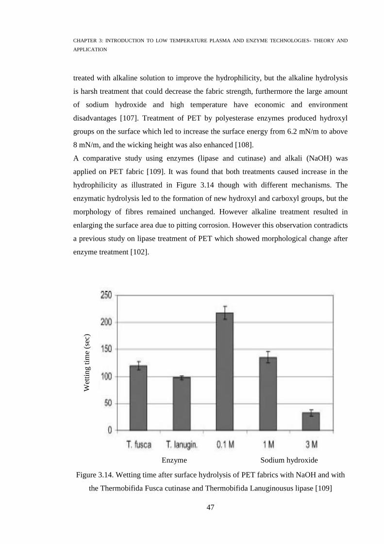
CHAPTER 3: INTRODUCTION TO LOW TEMPERATURE PLASMA AND ENZYME TECHNOLOGIES- THEORY AND
APPLICATION
47
treated with alkaline solution to improve the hydrophilicity, but the alkaline hydrolysis
is harsh treatment that could decrease the fabric strength, furthermore the large amount
of sodium hydroxide and high temperature have economic and environment
disadvantages [107]. Treatment of PET by polyesterase enzymes produced hydroxyl
groups on the surface which led to increase the surface energy from 6.2 mN/m to above
8 mN/m, and the wicking height was also enhanced [108].
A comparative study using enzymes (lipase and cutinase) and alkali (NaOH) was
applied on PET fabric [109]. It was found that both treatments caused increase in the
hydrophilicity as illustrated in Figure 3.14 though with different mechanisms. The
enzymatic hydrolysis led to the formation of new hydroxyl and carboxyl groups, but the
morphology of fibres remained unchanged. However alkaline treatment resulted in
enlarging the surface area due to pitting corrosion. However this observation contradicts
a previous study on lipase treatment of PET which showed morphological change after
enzyme treatment [102].
Figure 3.14. Wetting time after surface hydrolysis of PET fabrics with NaOH and with
the Thermobifida Fusca cutinase and Thermobifida Lanuginousus lipase [109]
Enzyme
s
Sodium hydroxide
Wet
ting t
ime
(sec
)

CHAPTER 3: INTRODUCTION TO LOW TEMPERATURE PLASMA AND ENZYME TECHNOLOGIES- THEORY AND
APPLICATION
48
A different result was reported on lipase treatment on PET film [95, 110]. No evidence
of PET hydrolysis was detected by HPLC, although the moisture regain was increased
after treatment. This was attributed to difference in morphology between PET films and
fabric, whereas the moisture regain increase was explained by possible change of pore
size and swelling which was not necessarily caused by enzyme action.
Modification of PLA fabric by lipase enzymes was reported to hydrolyse PLA fibres
which resulted in etching and improvement of the hydrophilicity [100]. Another
research on the enzymatic treatment of PLA fibre led to contradictive result with the
previous research. The study used various lipases and proteases from different origins
[111]. The effect of the treatment was assessed by weight loss, fibre strength and
morphology changes. All lipases used in this study had little or no ability to hydrolyze
PLA fabrics. On the other hand some of the proteases had remarkable activity for PLA
fabrics as demonstrated in Figure 3.15. The mechanism of action was not clearly
explained but it was attributed to the hydrolysis of ester bonds.
Figure 3.15. Weight loss of polylactic acid fabrics in enzyme solutions
Treatment time: one week, Concentration: 2 g/l [111]
Wei
ght
loss
(%
)
Enzyme

CHAPTER 3: INTRODUCTION TO LOW TEMPERATURE PLASMA AND ENZYME TECHNOLOGIES- THEORY AND
APPLICATION
49
Generally the above-mentioned review about enzyme treatment of polymers such as
PLA and PET indicated some contradiction in the results. It could be because the
biotechnology is still new for textile industry, and no standardised procedures and
conditions have been adapted so far. Another reason could be the sources where
enzymes originated and more research on the effects of enzymes origins should be
conducted.

CHAPTER 4: REVIEW OF VERTICAL WICKING AND SPREADING PROCESS AND THEORETICAL CONSIDERATIONS
50
Chapter 4
REVIEW OF VERTICAL WICKING AND SPREADING PROCESS AND
THEORETICAL CONSIDERATIONS
Chapter Overview
This chapter was assigned for reviewing the concepts of capillarity and kinetics of
wicking and wetting. It is divided into two parts:
Introduction to the basic principles and relationships governing capillary action
and the mechanisms of wicking.
Detailed explanation about vertical wicking and the spreading of micro drops.
4.1 Introduction
Wetting and wicking involve the interactions of a liquid with a solid, including the
formation of a contact angle at the solid/liquid interface, the spreading of a liquid over a
surface, and the penetration of a liquid into a porous solid medium. Wetting phenomena
is defined as the displacement a fibre-air interface with a fibre-liquid interface. Wicking
is the spontaneous flow of liquid through porous substrate driven by capillary forces
[112].
Wetting and wicking are ubiquitous in the natural and technological worlds. Examples
include droplet forming and rolling off plant leaves during insecticide spraying or the
self-cleaning of plant surfaces through rain or dew due to the interdependence between
water molecules and micro surface roughness which minimises the adhesion. They are
also of considerable interest in many technological processes such as sizing, de-sizing
[113, 114], printing [115], dyeing [116], textile finishing [117], and wear comfort [118].
Fluid flow through porous media is a complex subject found in many scientific fields
such as soil, physics, petroleum engineering, liquid filtration, paper chromatography,
textile testing. Over the years various theories and approaches have been developed to
study this area. The wicking behaviour of textile fabrics has been extensively studied
due to the paramount importance of wicking phenomenon and its connections with
textile processing and applications. In addition to this wicking can be used as a tool to

CHAPTER 4: REVIEW OF VERTICAL WICKING AND SPREADING PROCESS AND THEORETICAL CONSIDERATIONS
51
characterise fabric properties and test the reactions of fabrics to different textile
preparation processes.
Wicking can only occur when fibres assembled with capillary spaces between them are
wetted by a liquid. The resulting capillary forces drive the liquid into the capillary
spaces. An understanding of capillarity is therefore important in all textile wet
processes.
4.2 The Concept of Capillarity
Capillarity occupies a place in the general framework of thermodynamics in the context
of the macroscopic and statistical behaviour of interfaces rather than the details of their
molecular structure [119].The most common examples are liquid rise in capillary tube,
thin films, and drops formed by liquids in air or in another liquid. The following
sections present the fundamental factors that influence the capillarity.
4.2.1 Cohesive and Adhesive Forces
Cohesion is the mutual attractive force between like molecules of a particular liquid
which causes a tendency in the liquid to resist separation. Cohesive forces are
intermolecular forces such as hydrogen bonding and Van der Waals forces. An example
of a liquid which exhibits cohesive forces is water. Water is a polar molecule consisting
of partial positive charges on the hydrogen atoms and partial negative charges on the
oxygen atoms. These positive and negative charges are attracted to each other creating
cohesive forces which hold the water molecules together. Inside the bulk water, each
molecule is pulled evenly in every direction, whereas the molecules on the surface
lacking pulling forces in the outward direction, and experience an inward pull.
Therefore when water is spilled on a solid surface, it tends to form droplets, rather than
spreading out.
In contrast adhesion represents the attractive forces between unlike materials, such as
between a liquid and a solid container. When a liquid is put in contact with a solid
surface, the cohesive and adhesive forces govern the mechanism of the interaction
between the two substances, therefore the surface chemical compositions and
morphology play major role in polymer hydrophilicity and all other related properties.

CHAPTER 4: REVIEW OF VERTICAL WICKING AND SPREADING PROCESS AND THEORETICAL CONSIDERATIONS
52
4.2.2 Surface Tension
Cohesive forces between liquid molecules are responsible for the surface tension
phenomena as illustrated in Figure 4.1. The molecules at the surface do not have other
like molecules on all sides; consequently they cohere more strongly to those directly
associated with them on the surface. This forms a surface “film” which makes it more
difficult to move an object through the surface than to move it when it is completely
submersed. Phenomena such as the formation water drops, bubbles, and insect striders
walking on water surface (Figure 4.2) are all related to surface tension.
Figure 4.1. Graphical demonstration of the liquid molecules and surface tension [120]
Figure 4.2. Strider walking on the surface of water
Surface tension is referred to as the free energy per unit area, and it may equally well be
considered as the force per unit length. For example, consider a soap film stretched over
a wire frame for distance dx. If the value of the force per unit length is denoted by γ,
then the work done in extending the movable member a distance dx is

CHAPTER 4: REVIEW OF VERTICAL WICKING AND SPREADING PROCESS AND THEORETICAL CONSIDERATIONS
53
Work = γ.l.dx = γ.dA
l is the length of the frame (meter)
i.e. where dA is the change in area. The units of surface tension may therefore either be
ergs per square centimetre (ergs/cm2) or dynes per centimetre (dyn/cm). These are
identical dimensionally. The corresponding SI units are joules per square meter (J/m2)
or Newtons per meter (N/m). Surface tension values reported as dyn/cm and mN/m
have the same numerical value. Surface tension decreases with temperature as cohesive
forces decrease due to increase in molecular thermal activity. For example, the surface
tension of water at 22°C is 72.5 mN.m-1
, but it decreases to 62.6 mN.m-1
at 80°C [121]
[122]. Therefore hot water is a better cleaning agent because the lower surface tension
makes it a better “wetting agent” for access into pores. Also soaps and detergents
greatly lower its surface tension.
4.2.2 Contact Angle and Capillary Action
The contact angle, θ, is defined geometrically as the angle formed by the meniscus at
the three phase boundary where a liquid, air and solid intersect as shown Figure 4.3. It is
a quantitative measure of the wetting of a solid by a liquid. Low values of contact angle
(θ) indicate that the liquid spreads, or wets well, while a high contact angle indicates
poor wetting. If the angle θ is less than 90 degrees the liquid is said to wet the solid. If it
is greater than 90 degrees it is said to be non-wetting. A zero contact angle represents
complete wetting.
Capillary action is a spontaneous natural process, and is the tendency of fluids to rise in
narrow tubes or to be drawn into small openings such as those between grains of a rock.
This phenomenon is also sometimes described as capillarity. It is responsible for a large
number of natural behaviours, for instance how plants pull up the water from soil, or the
spontaneous sucking of liquid into a towel.
The relative strengths of cohesive and adhesive forces determine the direction of the
meniscus formed at the liquid-air interface and consequently the capillary rise. If
adhesive forces between the liquid and the solid surface are stronger than the cohesive

CHAPTER 4: REVIEW OF VERTICAL WICKING AND SPREADING PROCESS AND THEORETICAL CONSIDERATIONS
54
forces, the liquid is more attracted to the solid therefore the meniscus will concave up,
whereas if the cohesive forces of the liquid are stronger than the adhesive forces, the
liquid concaves down, in order to reduce contact with surface of the solid surface Figure
4.3.
Figure 4.3. Demonstrates the concave and convex meniscus [123]
4.2.3 Surface Tension and Contact Angle Relationship
The surface tension of a liquid tends to keep its surface to a minimum and restricts the
advancement of the liquid over the solid surface. For a liquid to wet a solid completely,
the solid surfaces must have sufficient surface energy to overcome the surface energy of
liquid. The forces involved in the equilibrium that exists when a liquid is in contact with
a solid and a vapour are demonstrated graphically in Figure 4.4. The relation between
these forces and contact angle is given by Equation 4.1 which is called the Young-
Dupre equation.
Equation 4.1
where γsl and γsv are the solid/liquid and solid/vapour interfacial tensions respectively
Concave up meniscus with contact angle
of less than 90°
Concave down meniscus with contact
angle of greater than 90°

CHAPTER 4: REVIEW OF VERTICAL WICKING AND SPREADING PROCESS AND THEORETICAL CONSIDERATIONS
55
Figure 4.4. Equilibrium state of a liquid drop on a solid surface [124]
The term γlv is sometimes referred to only by γ, and represents the surface tension of the
liquid-vapor interface. θ is the equilibrium contact angle. The Young-Dupre equation is
valid only for a drop resting at equilibrium on a smooth, homogenous, impermeable,
and non-deformable surface.
It has been found that solid surfaces with high surface tensions are more wettable than
those with low surface tension [125].
4.2.4 Effect of Roughness on the Capillarity
The effect of roughness on the capillarity was often correlated with study of the contact
angle. The Young-Dupre equation assumes that the surface in contact with the liquid is
smooth, isotropic and homogenous, and the contact angle given by this equation
referred to as the equilibrium contact angle. Solid surfaces such as textile fabrics are
rough and not homogenous. Wenzel [126, 127] discussed the influence of roughness on
the contact angle. It was argued that within a measured unit area of a rough surface
there is more surface than in the same measured unit area on a smooth surface, therefore
the interfacial tensions solid/vapour and solid/liquid should not be referred to the
geometric area, but to the actual surface area. The roughness factor (rw) was introduced.
rw is known as Wenzel’s roughness factor, defined as the ratio of the true area of a
surface (actually present on the microstructure of a surface) to the geometrically
projected area and given by Equation 4.2.

CHAPTER 4: REVIEW OF VERTICAL WICKING AND SPREADING PROCESS AND THEORETICAL CONSIDERATIONS
56
Equation 4.2
The relationship between the actual surface area and surface tensions was given by
Wenzel equation (Equation 4.4) as following
Equation 4.3
So this gives
Equation 4.4
Where:
is the equilibrium contact angle on the smooth surface
is Wenzel angle or the equilibrium contact angle on the rough surface
The roughness factor is always greater than unity, therefore Equation 4.4 predicts that
the Wenzel contact angle increases with roughness if the contact angle on a smooth
surface is greater than 90° and decreases if it is less than 90°. However this conclusion
seemingly conflicts with experimental observations; one finds that with increasing
roughness, the advancing contact angle always increases and the receding contact angle
decreases [128].
The Wenzel equation does not describe the contact angle hysteresis and hence the
relationship between the roughness and hysteresis. The surface roughness can produce
contact angle hysteresis. Figure 4.5 shows schematically the expected behaviour of the
advancing and receding contact angles as a function of roughness for surfaces whose
equilibrium contact angle on the corresponding smooth surface is lower and greater than
90º. In both cases the advancing angle increases and the receding angle decreases as
roughness increases. But in surfaces whose angle is lower than 90º, above a certain
degree of roughness, depending on the roughness dimensions and geometry, wettability
becomes a capillary phenomenon, and wicking promoted by capillarity occurs, resulting

CHAPTER 4: REVIEW OF VERTICAL WICKING AND SPREADING PROCESS AND THEORETICAL CONSIDERATIONS
57
in a decrease in contact angle. On the other hand, on hydrophobic surfaces characterised
by > 90º, the liquid can no longer penetrate the surface, and the drop of liquid is in
contact with a surface composed in part by the solid and in part by air [129].
Figure 4.5. Theoretical behaviour of advancing and receding angles as a function of
roughness a) <90, b) >90 [129]
4.3 Wicking in Textile Materials
Textile wicking is the transport of moisture or liquid within a fabric under the influence
of capillary action. Wicking can occur in one dimension such as vertical wicking, or in
two dimensions like the spreading of a drop of liquid. Wicking plays important role in
textile processes such as dyeing and printing and applications such as wear comfort. In
active sportswear wicking mechanism disperses perspiration throughout the fabric
which results in rapid evaporation of perspiration and body vapour so the wearer stays
dry and comfortable [130 – 133]. [130] [131] [132] [133].
Textile preparations, dyeing and finishing processes involving usage of surfactants and
chemical agents are also correlated with wicking ability. Wicking tests are also being

CHAPTER 4: REVIEW OF VERTICAL WICKING AND SPREADING PROCESS AND THEORETICAL CONSIDERATIONS
58
used to study liquid-substrate interactions, and to evaluate the effects of textile
preparation processes such plasma, enzyme and alkaline treatments on the modifications
of properties and the behaviour of textile materials.
Due to the importance of wicking behaviour, many researches have been conducted to
investigate and analyse the wicking of different textile materials [134, 135]. Recently
textile products with enhanced wicking properties have entered the market, such as
WICKING WINDOWS by Cotton Incorporation [136], TOREX® FIELDSENSOR®
by Toray Company [137], and COOLMAX by INVISTA [138].
Wet textile processes are time dependant; therefore it is necessary to know how the rate
of wicking changes over time, which is usually known as the wicking rate [112].
Wicking behaviour depends on the surface tension and viscosity of the liquid; it also
depends on the capillary dimensions of the substrate [139]. The shape of the fibres in an
assembly such as a yarn or a fabric affects the size and geometry of the capillary spaces
between fibres, and consequently the rate of wicking.
The term wicking has been used sometimes in the literature to study two different
processes: the spontaneous flow of a liquid within the capillary spaces, and the
spontaneous flow of the liquid within capillary spaces accompanied by a simultaneous
diffusion of the liquid into the interior of fibres [140]. If liquid does not penetrate into
the fibre the wicking process is termed capillary penetration. When the liquid diffuses
into the fibre, it causes swelling [141], reduces the capillary spaces between fibres, and
complicates the kinetics [142]. However for clarification wicking processes can be
divided into four categories depending on the interaction mechanism between liquid and
fibre [112].
1- Wicking of a liquid- no significant diffusion into the fibre. In this case, capillary
penetration is the only process operating e.g. hydrocarbon oil wicking in a
polyester fabric at ambient temperature.
2- Wicking accompanied by diffusion of liquid into fibres or into a finish on the
fibre. Two simultaneous processes occurs together capillary penetration and
diffusion of liquid into the fibres e.g. water wicking in a cotton fabric and
diffusing into fibres.
3- Wicking accompanied by adsorption on fibres (there is no diffusion of liquid
into fibre) e,g an aqueous surfactant solution wicking in polyester fabric.
CHAPTER 4: REVIEW OF VERTICAL WICKING AND SPREADING PROCESS AND THEORETICAL CONSIDERATIONS
59
4- Wicking involving adsorption and diffusion into fibres, e.g., an aqueous
surfactant solution wicking in a cotton fabric. Several processes are operating
simultaneously, capillary penetration, diffusion of the liquid into the fibres, and
adsorption of the surfactant on fibres.
4.3.1 Wicking Kinetics
In order to study the wicking behaviour in textiles, fibrous assemblies are considered as
number of parallel capillaries [143]. Kissa [112] assumed that fibrous materials
constitute non-homogenous, irregular and discontinuous capillary systems; therefore the
liquid transport through fibrous materials occurs in small jumps. The advancing wetting
line stretches the meniscus of liquid until the elasticity of the meniscus and the inertia of
flow are exceeded. Then the meniscus contracts, pulling more liquid into the capillary to
restore the equilibrium state of the meniscus. The flow in a capillary may stop when the
capillary allows the meniscus to reach an edge and flatten [144].
Based on the type of reservoir which supplies the substrate, the wicking process can be
categorised as wicking from an unlimited or limited reservoir.
4.3.1.1 Wicking from an Unlimited Reservoir
Wicking from an unlimited reservoir includes the following wicking categories:
Immersion
Trounson et al. [145] reported that wicking during immersion occurs when the fabric (or
fibrous assembly in general) is completely immersed in a liquid and the liquid enters the
fabric from all directions. A liquid wicking into an immersed yarn or fabric displaces
most of the air in fibrous assembly and causes it to sink.
Longitudinal or In-plane Wicking
It is common practice to use in-plane wicking measurements to evaluate the absorbing
power or liquid transport capabilities of fibrous sheet materials.
The usual test method for longitudinal wicking is the vertical wicking test. Details about
this test are provided in paragraph (4.5).
Transverse Wicking
Transverse wicking is the transport of a liquid through the thickness of a fabric, in a
direction perpendicular to the plane of the fabric, such as the mechanism of water
uptake by towel, also known as “transplanar liquid uptake” [146]. The importance of

CHAPTER 4: REVIEW OF VERTICAL WICKING AND SPREADING PROCESS AND THEORETICAL CONSIDERATIONS
60
transverse wicking is that it simulates the mechanism of liquid perspiration movement
through fabric thickness. Transverse wicking is more difficult to measure than
longitudinal wicking as the distances involved are very small and hence the time taken
by a liquid to transverse the thickness of fabric is short.
4.3.1.2 Wicking From a Limited Reservoir
The wicking from a limited reservoir is usually simulated by a drop test. The test can be
applied to a single fibre, yarn, filament or fabric using different drop volumes. Either
the drop spreading rate [147, 148], or drop absorbency time [149, 150] was measured.
The capillary penetration of a drop indicates several important properties of a textile
fabric, including repellency, absorbency, and stain resistance [151, 152]. Also the
wicking of minute drops of liquid in a fabric has become very important for inkjet
printing technology [153]. This test is explained in detail in paragraph (4.6) and
involves measuring the spreading rate.
4.4 Vertical Wicking
4.4.1 Theoretical Background
Textile materials such as knitted and woven fabrics, paper towels, fluff pads, have
complex structures. The capillaries are neither cylindrical nor arranged in parallel.
Capillary flow through textile materials can be studied by a capillary tube model which
considers the textile substrate as an assembly of very small capillaries as shown in
Figure 4.6.

CHAPTER 4: REVIEW OF VERTICAL WICKING AND SPREADING PROCESS AND THEORETICAL CONSIDERATIONS
61
Figure 4.6. Capillary representation of a textile fabric
In a capillary, liquid rises due to the pressure drop (ΔP) across the liquid-air interface.
The pressure drop can be expressed by Equation 4.5.
ΔP=P- ρgh Equation 4.5
Where:
ρ is liquid density (g/cm3)
g is gravitational acceleration constant (980.7 cm/sec2)
h is the height of liquid rising (cm)
In an idealised tube, the capillary pressure P is described by Equation 4.6, also called
Laplace pressure [119], where Fwt is the internal wetting force which represents the
vertical component of liquid surface tension γ around the perimeter of the tube. The
internal wetting force is given by
Equation 4.6
where:
is the liquid surface tension of liquid-air interface (mN/m)
Rs is the radius inside the capillary, also called the radius of dry capillary

CHAPTER 4: REVIEW OF VERTICAL WICKING AND SPREADING PROCESS AND THEORETICAL CONSIDERATIONS
62
θ is the contact angle
This equation indicates that yarn with smaller contact angle, creates a larger capillary
pressure and the capillary pressure is inversely related to the capillary radius, so the
smaller the radius the higher the pressure.
When the capillary pressure is greater than the hydrostatic pressure, which represents
the weight of liquid (ρgh), a positive force drives the liquid upward. Equation 4.5 can
then be written
Equation 4.7
The velocity of laminar flow, through an ideal tube with constant cross section, can be
stated according to Hagen-Poiseuille law [154, 155] as shown in Equation 4.8.
Equation 4.8
where:
q is the velocity of flux (m/sec)
Rw is the mean hydrodynamic radius of pores or also called radius of wet capillary
η is the viscosity of liquid (cP)
ΔP the pressure drop across the distance (h)
The Hagen-Poiseuille law indicates that the velocity is proportional to the square power
of the radius, and inversely proportional to the length of the tube. Substituting Equation
4.7 in Equation 4.8 results in Equation 4.9

CHAPTER 4: REVIEW OF VERTICAL WICKING AND SPREADING PROCESS AND THEORETICAL CONSIDERATIONS
63
Equation 4.9
The effect of a change in surface tension on the capillary transport rate is difficult to
predict since a decrease in surface tension is expected to increase (except when θ
= 0) according to Equation 4.1. However, Nutter [156] reported that the addition of
surfactant, with the consequent reduction in surface tension, leads to an increase in
transport rate.
At an early stage of liquid rising, the hydrostatic pressure can be neglected, so Equation
4.9 can be written
Equation 4.10
The ratio
called the effective capillary radius Re
Integrating Equation 4.10 yields Equation 4.11
Equation 4.11
This equation is applicable at early stages of liquid rise, where h is smaller than the
equilibrium height, otherwise it will give wrong assumption that the flow is indefinite.
Equation 4.11 is known as the modified Washburn equation, because Washburn
assumed that Rw and Rs are the same, but a later study suggested the radius of Equation
4.8 is a wet capillary radius whereas in the Laplace equation it is a dry capillary [157]. It
predicts that liquid penetration is proportional to the square root of time, and the rate of
penetration increases with increasing size of effective capillary, decreasing viscosity
and increasing surface tension. Various methods can be used to modify the wicking rate,
such as adding surfactant, plasma and enzyme treatments. Equation 4.11 can be written
as Equation 4.12.

CHAPTER 4: REVIEW OF VERTICAL WICKING AND SPREADING PROCESS AND THEORETICAL CONSIDERATIONS
64
Equation 4.12
Where
Wc is referred to as the wicking coefficient [158]. It is related to the liquid properties η,
γ, the interaction between liquid and fabric θ. Wc is commonly used to evaluate the
wicking rate of different materials.
When equilibrium is reached, the upward capillary driving force P equals the weight of
the column of liquid; the net force on the liquid is zero and the rising of the liquid stops.
The equilibrium capillary rise can be expressed as:
Equation 4.13
In the case where hydrostatic pressure cannot be neglected, at equilibrium Equation 4.9
can be written as Equation 4.14
Equation 4.14
Integration of this equation leads to Equation 4.15.
Equation 4.15
4.4.2 Anomalies of Wicking Behaviour in Textiles
Textile materials are porous media with much more complex structures than ordinary
capillary tubes. The pores in such structures are often interconnected void spaces,
having different sizes, and distributed unevenly throughout the structure. Therefore the
fluid has to follow tortuous paths. Also, due to the different sizes of pores, the fluid

CHAPTER 4: REVIEW OF VERTICAL WICKING AND SPREADING PROCESS AND THEORETICAL CONSIDERATIONS
65
located at partially saturated regions will experience a multitude of different “pulls”
from different pores.
Various research groups used the Washburn approach to calculate the wicking rate and
contact angle [159, 160]. There are two issues which need to be clarified in relation to
textiles. First, if liquid influences the capillary dimension, the time and advancing
distance relationship is not as predicted by Equation 4.11 and Equation 4.12. This
situation may rise if the structure is composed of a highly swellable type of fibre. As
wicking proceeds in the structure, water continuously diffuses into the fibre structure
resulting in a continuous change of the dimension of the wet capillaries as a function of
time. To some extent, all natural fibres swell in water and the swelling is always time
dependant; therefore Re is never a constant factor. However, as a first approximation, Re
may be considered a constant if the degree of swelling is not high. To test
experimentally how closely the modified Washburn equation is applicable to the
mechanism of wicking of a certain fabric, a plot (log h vs log t) should be linear with a
slope of approximately 0.5, as long as the height h is smaller than the equilibrium level.
The second issue, the Washburn, Hagen-Poiseuille, and Laplace equations, were derived
assuming specific conditions of laminar flow and idealised circular conduit (tube or
pipe). In practical applications such as knitted fabric, the flow is turbulent and should be
described by a more rigorous model which considers the inertia, frictional properties
and material specifications [161 - 163].[161] [162] [163].
The Washburn equation was accepted for use in the study of vertical wicking in this
research as a mathematical model for comparison between the treated and untreated
fabrics, because the purpose of this investigation was to examine the effect of various
preparation processes on the wicking behaviour rather than studying the detailed factors
affecting the wicking.
4.6 Spreading Dynamics of Micro Drops through Textile Materials
4.6.1 Introduction
The spreading process is simply defined as a wicking mechanism; it is different from
vertical wicking because the liquid moves in two dimensions and is supplied from a
limited reservoir.

CHAPTER 4: REVIEW OF VERTICAL WICKING AND SPREADING PROCESS AND THEORETICAL CONSIDERATIONS
66
In most wet processing of fibrous materials, uniform spreading and penetration of
liquids into pores are essential for the best performance of the products. The spreading
dynamics of a liquid in a fibrous material and other solid surfaces plays a key role in
many practical processes. The quality of an inkjet print image can be predicted by
analysing the spreading of the drops over the fabric surface [164, 165], as well the
mechanism of detergent solution spreading over fibre [166, 167] and using the softening
agent [168].
The capillary spreading measurements are an effective tool in comparing the
hydrophilicity of fabrics and characterising fabric surface properties. Though there
have been studies on the spreading of micro drops on solid surfaces, the physics
underlying the spreading of a liquid on a solid surface has remained poorly understood
until recently and some issues remain controversial [169]. In fact, concerning textile
fabrics little research has been carried out on the spreading.
The problem of a drop spreading in textile materials is correlated to the spreading
behaviour of liquids in other non-textile materials such as papers, sand and soil,
therefore the results of this research may be of use in studies of other subjects.
4.6.2 Kinetics of Drop Spreading
The main force which drives a liquid during spreading is related to the capillary force
which is generated between fibres. The values of these forces depend on the "capillary
diameter", which in a fabric is related to distance between the fibres. The drop weight or
the gravity helps the liquid to penetrate into the textile structure. Forces which act
against liquid spreading belong to viscous forces, which can play significant role in very
small spaces between fibres. Therefore from a theoretical point of view the final fluid
distribution depends on:
1. Capillary force parameters:
a) contact angle
b) surface tension
c) distance between fibres, yarn torsion, yarn packing and fabric structure.
d) fibre diameter, yarn diameter.
2. Viscous forces
3. Over a large spreading time there is an effect related to drying, which decreases the
wicking length.

CHAPTER 4: REVIEW OF VERTICAL WICKING AND SPREADING PROCESS AND THEORETICAL CONSIDERATIONS
67
4.6.2 Theoretical Background
Studies of the spreading process date back to 1956 when Gillespie [147] first
established a method to observe liquid drops through filter paper. Gillespie attempted to
find a mathematical relation between drop volumes and areas. The apparatus used in the
study is shown in Figure 4.7. The apparatus consisted of microscope, and a syringe
mounted 1cm above the filter paper to place the drop.
Figure 4.7. Schematic diagram showing the apparatus made by Gillespie to observe the
liquid movement [147]
The dynamic diameter of the spot was measured at various time intervals. Also the
distribution of the liquid was measured optically. Gillespie tested the spreading of
different liquids on the same substrate to assess the influences of liquid properties on
the spreading process. Figure 4.8 expressed the variation of stain radius (R) with time
for various liquids spreading on Whatman filter paper no.1. Also, the spreading of the
same liquid (dibutyl phthalate) on different filter papers and print cards was investigated
to evaluate the effect of substrate properties, as shown in Figure 4.9.

CHAPTER 4: REVIEW OF VERTICAL WICKING AND SPREADING PROCESS AND THEORETICAL CONSIDERATIONS
68
Figure 4.8. Relationship (R, Time) of spreading of different liquids as reported by
Gillespie. D.B.P dibutyl phthalate [147]
Figure 4.9. Spreading of dibutyl phthalate in various grades of filter papers and printflex
cards [147]

CHAPTER 4: REVIEW OF VERTICAL WICKING AND SPREADING PROCESS AND THEORETICAL CONSIDERATIONS
69
Gillespie concluded that the spreading process could be split into two phases,
demonstrated in Figure 4.10 . In the first there is some of the liquid remaining on the
surface of the substrate in form of a flattened drop; in the second all the liquid is
contained within the paper.
Figure 4.10. Spreading phases as suggested by Gillespie [147]
The changes in the mechanism of spreading between the first and the second phases can
be explained kinetically by the energy change which drives the liquid movement. In the
first phase it is assumed that there is a gravity effect plus capillary action, while in the
second phase there is only capillary action.
Gillespie suggested that as the first stage is usually completed in a relatively short time,
it could be ignored or considered of secondary importance in drop spreading. The
observations and analysis of the second phase led to the finding that the relation
between drop volume and area during the second phase can be expressed by empirical
Equation 4.16.
Equation 4.16
Where:
R denotes the radius of the stain (mm)
R0 is the radius of the stain at time zero (mm)
V is the volume of the liquid (mm3)
h is the thickness of the substrate.

CHAPTER 4: REVIEW OF VERTICAL WICKING AND SPREADING PROCESS AND THEORETICAL CONSIDERATIONS
70
The coefficient β was given by Equation 4.17
.
cos...3
s
s
C
qb Equation 4.17
Where:
b is constant descriptive of the substrate, though it was not clearly identified
qs is the permeability of the substrate
γ is the surface tension
η is the viscosity of the liquid
θ is the advancing contact angle
Cs is the saturation concentration of the liquid in the substrate
Gillespie noticed that in some papers the liquid tended to spread more easily in one
direction than in others. In these cases the stain diameters were assessed in two
directions, one parallel and one normal to the preferred direction, when the difference
was >10%.
Later in 1981 Kissa [148] studied the spreading of drops through textile materials.
Unlike papers, textile fabrics are not isotropic, the area of a stain formed by a liquid
drop on a textile fabric is not a perfect circle, therefore rather than measuring the
diameter, Kissa measured the total area covered by the spreading liquid. After placing a
drop on fabric it disappears and moves very quickly, so Kissa devised a photographic
machine for the instantaneous measurement of drop movement. A syringe was used to
place the drop onto the substrate. A schematic representation of the device is shown in
Figure 4.11.

CHAPTER 4: REVIEW OF VERTICAL WICKING AND SPREADING PROCESS AND THEORETICAL CONSIDERATIONS
71
Figure 4.11. Device developed by Kissa for measuring of drop spreading [148]
Kissa measured the spreading of a drop as a function of time. The area of the spreading
liquid at given times were photographed simultaneously with an instant-picture camera.
The area depicting the spread liquid was cut out from the dried photograph and
weighed, then converted to unit area.
To determine the weight of unit area (1cm2), a known size area was photographed and
weighted. The precision of the method was determined by photographing the known
area eight times. The standard deviation of 49 cm2 of area photographed eight times was
found to be 0.4 cm2. Kissa applied the experiments on cotton, polyester, and a cotton-
polyester blend. Also he tried a variety of liquids with drop volumes ranging between
0.05-0.5 ml.
It was assumed that the fibres were impermeable to the spreading liquid. Equation 4.16
derived by Gillespie for the second phase of spreading, can be written in the following
form
Equation 4.18

CHAPTER 4: REVIEW OF VERTICAL WICKING AND SPREADING PROCESS AND THEORETICAL CONSIDERATIONS
72
where:
A is the area covered by the spreading liquid
A0 is the area at time zero.
K is the capillary sorption coefficient given by Equation 4.19
Equation 4.19
According to Equation 4.18 the difference is proportional to t/A when K, γ and
h are constants.
Equation 4.20
For an example, Kissa plotted the relation (A2, t/A) of the spreading of dodecane in
polyester/cotton fabric as shown in Figure 4.12. The graph indicates that the spreading
process consists of three parts, two phases of spreading and the equilibrium level where
the liquid spreading has stopped. The main part of the curve, representing spreading of a
liquid completely within the fabric, which is the situation of second phase, is linear in
accordance with Equation 4.20.

CHAPTER 4: REVIEW OF VERTICAL WICKING AND SPREADING PROCESS AND THEORETICAL CONSIDERATIONS
73
Figure 4.12. Spreading of 0.10 ml of n-dodecane on dyed polyester/cotton fabric [148]
The straight line intercepts with the A2
axis at Ai2, so the straight line can be expressed
Equation 4.21.
A
tVKAA i
222
Equation 4.21
This equation can be written:
tVK
AAA i
223 .
Kissa concluded that the Gillespie equation can be applied for textile fabrics during the
second phase of spreading, but he suggested that A0 can be neglected because it is very
small relative to the area A. Also to simplify the equation, Ai could be neglected, but the
slope of the curve has to be adjusted to fit the experimental data. The area A is
expressed by Equation 4.22.
33.067.033.0)/( tVKA Equation 4.22
Equation 4.22 can be written in the general form expressed as Equation 4.23

CHAPTER 4: REVIEW OF VERTICAL WICKING AND SPREADING PROCESS AND THEORETICAL CONSIDERATIONS
74
nmu tVKA )/( Equation 4.23
The exponents in Equation 4.23 are expected to deviate from those shown in Equation
4.22 due to neglecting the value of Ai , but the deviation is not large.
The value of the exponent n can obtained from the slope of the curves from the
logarithmic plots of the area covered by liquid A as a function of time t. The value of m
can be obtained from the logarithmic plot of the area at 1 minute (A1) as a function of
the volume of the liquid drop V. Finally, the value of the exponent u can be obtained
using the known values of V and m.
Another example proposed by Kissa to prove his theory is the spreading of n-decane on
polyester and polyester-cotton fabrics shown in Figure 4.13.
Figure 4.13. Logarithmic plot of the areas covered by n-decane on polyester and
polyester-cotton blend fabrics as a function of time (V = 0.10 ml) [148]
In the previous discussion, the fibres were assumed to be impermeable to the liquid. If
the fibres can absorb the liquid, the volume of free liquid in the fibrous capillaries
reduces and the fibres swell, resulting in decreased capillary spaces. On the other
hand, liquids absorbed by the fibres can be expected to wet the fibre surface. The
advancing contact angle should therefore be small, leading to favourable conditions

CHAPTER 4: REVIEW OF VERTICAL WICKING AND SPREADING PROCESS AND THEORETICAL CONSIDERATIONS
75
for capillary spreading.
Kissa’s study on the kinetics of liquid spreading through permeable fibres concluded
that this process depends on the liquid and fibre properties as well as the drop volume.
For example, for the spreading of water on cotton fabric, the exponent n increased
from 0.08 to 0.20 when the drop volume was increased from 0.10 to 0.40 ml. Also it
was noticed that water covers a smaller area on cotton fabric than an equal volume of
dodecane at equal spreading times.
Drop spreading on textile materials has been followed by Kawase [151]. He examined
the spreading of liquids through impermeable and permeable fibres, and investigated
the applicability of Equation 4.23. Figure 4.14 illustrates the apparatus used in the
experiments. It consists of a desicator with a 200 mm diameter, video camera and
micropipette. The fabric was mounted on wooden ring. A measured amount (0.05 to
0.20 ml) of liquid was introduced onto the fabric. The area of the spread liquid and the
stopwatch were recording simultaneously on a videotape. The temperature of the
apparatus was maintained at 25°C throughout the experiment. The spreading area was
copied on the film, cut out, and weighed. A calibration curve was determined by
recording the areas of several known sizes and weighing the copied film in every
experiment in order to determine the actual spreading area.
Figure 4.14. Apparatus made by Kawase to study liquid spreading [151]
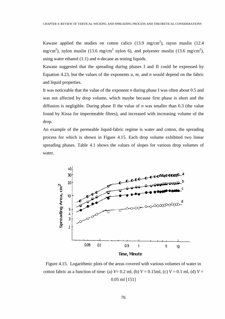
CHAPTER 4: REVIEW OF VERTICAL WICKING AND SPREADING PROCESS AND THEORETICAL CONSIDERATIONS
76
Kawase applied the studies on cotton calico (13.9 mg/cm2), rayon muslin (12.4
mg/cm2), nylon muslin (13.6 mg/cm
2 nylon 6), and polyester muslin (13.6 mg/cm
2),
using water ethanol (1:1) and n-decane as testing liquids.
Kawase suggested that the spreading during phases I and II could be expressed by
Equation 4.23, but the values of the exponents u, m, and n would depend on the fabric
and liquid properties.
It was noticeable that the value of the exponent n during phase I was often about 0.5 and
was not affected by drop volume, which maybe because first phase is short and the
diffusion is negligible. During phase II the value of n was smaller than 0.3 (the value
found by Kissa for impermeable fibres), and increased with increasing volume of the
drop.
An example of the permeable liquid-fabric regime is water and cotton, the spreading
process for which is shown in Figure 4.15. Each drop volume exhibited two linear
spreading phases. Table 4.1 shows the values of slopes for various drop volumes of
water.
Figure 4.15. Logarithmic plots of the areas covered with various volumes of water in
cotton fabric as a function of time: (a) V= 0.2 ml, (b) V = 0.15ml, (c) V = 0.1 ml, (d) V =
0.05 ml [151]

CHAPTER 4: REVIEW OF VERTICAL WICKING AND SPREADING PROCESS AND THEORETICAL CONSIDERATIONS
77
Table 4.1. Values of exponent n during phase I and II for spreading of water in cotton
fabric [151]
Volume of drop V ml Value of n
Phase I Phase II
0.05 0.504 0.102
0.100 0.494 0.118
0.150 0.501 0.137
0.200 0.497 0.145
Studies on an impermeable fibre-liquid system such as polyester and n-decane,
exhibited approximately constant values for slopes n with various drop volumes, during
the first and second phases as demonstrated in Table 4.2. This proved that the drop
volume has no effect on the rate of spreading when using an impermeable fabric.
Table 4.2. Values of exponent n during phase I and II for spreading of n-decane in
polyester fabric [151]
Volume of drop V ml Value of n
Phase I Phase II
0.05 0.495 0.293
0.100 0.496 0.301
0.150 0.502 0.300
0.200 0.508 0.299
Kawase investigated the effects of fabric preparation by softening agents on the wetting
of textiles by measuring the capillary spreading of liquid as a function of time. The
values of the exponent n of permeable fibres during phase II of the capillary spreading
over softened fabrics increased in comparison with those of un-softened fabrics, owing
to the adsorption of the softening agent, which made the fibre surface more
hydrophobic, resulting in larger volume of liquid to spread.
Research into the spreading of drops on textile fabrics was also conducted by Nutter
[156]. He studied the spreading of various solutions of dye on plain woven cotton. The
device he used is shown in Figure 4.16. The camera was mounted below the fabric to

CHAPTER 4: REVIEW OF VERTICAL WICKING AND SPREADING PROCESS AND THEORETICAL CONSIDERATIONS
78
snap the images of the spreading process at different time intervals up until the liquid
movement had stopped. The images were taken off the negative film and projected on
paper to be enlarged for accurate measurement. The drop was formed gradually until
reaching critical weight, when it fell on the fabric. At this moment the first photograph
was taken.
Figure 4.16. The spreading device used by Nutter [156]
Nutter measured the radius of the drops, and assessed the effect of drop mass on final
stain radius. The relation between spreading area and time was represented by an
asymptotic curve shown in Figure 4.17. It exhibited very high rate of initial spread,
gradually approaching a rate of zero. It was found that the relationship between drop
mass and final area of spreading could be expressed by the following empirical linear
Equation 4.24
Equation 4.24
Where:
A is final spreading area
M is the drop mass
C and k are constants, 0.3 and 148 respectively.

CHAPTER 4: REVIEW OF VERTICAL WICKING AND SPREADING PROCESS AND THEORETICAL CONSIDERATIONS
79
Time (second)
Figure 4.17. Dye solution spreading over cotton fabric
(Drop mass=44.2 mg dye solution) [155]
A more recent study of liquid transport through textile materials has been done to relate
the quality of ink jet printing with liquid drop spread [165]. Experiments on drop-
spreading kinetics were performed using the set up shown in Figure 4.18. The drop
spreading process was found to simulate the inject drop, and could be used as predictor
for the printing quality.
Figure 4.18. Instrument used to observe the drop spreading [165]
Spre
adin
g a
rea
(cm
2)

CHAPTER 4: REVIEW OF VERTICAL WICKING AND SPREADING PROCESS AND THEORETICAL CONSIDERATIONS
80
4.6.3 General Observation of the Previous Studies
The mathematical model derived by Kissa is an empirical relationship. It can perform
well, but probably only in some restricted domains of fluid and textile parameters. For
example it does not explain the effects of textile geometry (twill, yarn count and others)
which have large influences on the final fluid distribution.
In the study carried out by Nutter [156], measuring the radius of the drop is not accurate
for textile materials, because seldom does the stain area form a perfect circle. Also
Equation 4.24 is not clear. As it was reported, this equation does not hold in the case of
small drops as the relation becomes nonlinear, and there was no clear explanation about
the drop size he used.
Mhetre [165] used Kissa equation to measure the spreading rate, but as mentioned
above there are some reservations about using this equation. Mhetre found the spreading
process can be used to predict printing image quality.
CHAPTER 5: EQUIPMENT AND PROCEDURES
81
Chapter 5
EQUIPMENT AND PROCEDURES
Chapter Overview
This chapter documents the equipment and procedures which were used to carry out the
research. As well it defines the terms and methodologies which are used to analyse the
results.
5.1 Europlasma CD400
This plasma is categorised as low pressure plasma, provided with radio frequency
generator CESARTM
Model 1310, frequency 13.56 MHz, power operation range 80 -
600 Watts, and vacuum pump to evacuate the chamber prior to the treatment. The inlet
gas is controlled by mass flow controller, via which the pressure is controlled inside the
chamber therefore the flux values is given.
The machine has the capability of treating flat samples as well as rolls of fabric and or
yarn. It can be operated either fully automatically with a programme created using the
machines integrated software or manually. Two gases can be connected to the unit
simultaneously as shown in Figure 5.1. In this research the machine was operated using
the automatic mode and programmes were set up according to the condition given in
Table 7.2. Each treatment cycle starts with reducing the pressure to the vacuum level
known as base pressure (100 mbar) to evacuate all the gases out of the chamber, and
then the treatment gas is released into the chamber, resulting in increase the pressure to
“work pressure”, and the power starts to activate the plasma.

CHAPTER 5: EQUIPMENT AND PROCEDURES
82
Figure 5.1 Schematic diagram of Europlasma CD400 operation system
5.2 Nanotech Plasma PE250
This plasma machine is also low pressure plasma, equipped with radio frequency
generator model OEM-6, serial 729, with power range 25-60 Watts. This machine is
semi-automated. Before the treatment the vacuum pump turns on to evacuate the
chamber, and the system is flushed with argon gas to purge out any other gases. Then
the flow meter is set up; the pressure is adjusted by manual gauge. Lastly the RF power
turns on and adjusted to required level.
5.3 Conditioning the Specimens
The properties of fibres vary with the moisture condition; dry fibre has a lower linear
density and a smaller diameter than a wet one [170]. Testing should be done under
controlled conditions. For this purpose, a standard temperature atmosphere is defined as
one of 65% r.h. and 20 °C [171]. The permitted tolerances for testing are ± 2% r.h
(relative humidity) and ± 2 °C.

CHAPTER 5: EQUIPMENT AND PROCEDURES
83
5.4 Vertical Wicking Test
The purpose of this test is to characterise the fabric ability in terms of capillary flow,
and to assess the consequences of surface modification via plasma treatments.
The standard methods for wicking tests are BS 3424 Method (1971) and DIN 53924
(1997). The former method specifies a very long time period (24 hours) and is intended
for coated fabrics with very slow wicking performance. In contrast, DIN 53924 is
appropriate for relatively rapid wicking fabrics. It specifies a shorter time for the test,
about 5 minutes, and requires the liquid height to be recorded every 15 seconds [172].
These standards specify the basic principles for testing. They can be modified to adapt
new technologies such as the use of a high definition camera and implementation of
image analysis, provided that the conditions of test are documented and given along
with the results.
Various techniques have been developed and used to study vertical wicking in textile
fabrics, such as measuring the height of liquid rise, or the liquid mass absorbed by a
fabric, or using electrical sensors to detect the liquid motion [173, 174].
In this research the coloured liquid height was observed as it fulfils the study
requirement of comparing the effects of various kinds of textile preparations on liquid
transport. A solution of distilled water coloured with C.I. Acid Blue 25 (0.2 g/l) to make
it easier to observe the liquid movement by the camera. An acid dye was chosen
because it was assumed to have no affinity for the fibre.
The surface tension (γ) of the liquid was measured using a Kruss Tensiometer K6 device
under standard conditions. It was found to be around 62 mN/m, in comparison to the
value for pure distilled water of 71 mN/m. This could be correlated with adding dye to
the water as it has been shown to reduce the surface tension [175]. The viscosity of the
liquid was η = 1.23 cP, measured by Brookfield DV-II + Pro viscometer.
Figure 5.2 shows the vertical wicking device. Test sample is fabric strip 2 × 17 cm.
To carry out the test a Petri dish was filled with the testing liquid. The lower end of the
strip was immersed 1 cm in the liquor.
The movement of solution through the fibrous material was recorded using a digital
camera. Imagegrab software was utilised to grab the frames.

CHAPTER 5: EQUIPMENT AND PROCEDURES
84
Figure 5.2. demonstration of wicking process through PLA fabric strip
5.6 Spreading Test
This research worked to develop the technique of measuring accurately the spreading of
drops through textile fabric. Section 4.6 presented a review of all previous work made
in this area. The further developments achieved in this study were:
1- Testing of a smaller drop size of 12.5 micro litres, and the ability to observe the
liquid movement within a fraction of a second.
2- Utilisation of image analysis which helped obtaining accurate and faster
measurements.
3- Measuring the dynamic change of the shape of stain area. As the percentage of
100 % circular area.
Figure 5.3 shows the device for measuring the spreading rate. The system consisted of
high speed video camera (Altra 20, 1.5 megapixel), mounted on stereomicroscope
equipped with a C-mount and LED light, and connected to a personal computer.
The camera stage is moveable, and fixtures are used to adjust the distance between the
camera and the sample. The substrate was glued without any applied tension to flat
frame holder made of paperboard (thickness 1mm) shown in Figure 5.4. This holder

CHAPTER 5: EQUIPMENT AND PROCEDURES
85
offers stretch-free and uniform setting. The height between the tip of the needle and the
stage of the microscope is 1 cm.
Micro driver syringe pump (KDS 100), Hamiltone syringe (100 µl), and needle with flat
tip were used to form the drop. The needle was tilted to let the drop fall vertically, this
position gives smallest drop volume possible with this equipment. The speed of the
driver is 1000 µl/h; the drop of the solution takes approximately 45 seconds to form and
fall, which makes the drop volume of 12.5 µl.
Image analysis software “ANALYSIS 5” was used to measure the spot area and the
roundness of the spot. The area of the spot was measured by using the Free Hand tool of
the software, each spot was measured three times, and average value was taken. The
microscope and the camera was calibrated using graticule. In order to obtain
reproducible results the conditions of the experiment were kept constant, including
lighting, temperature, humidity. The liquid used in this test is the same described in the
vertical wicking test. In theory the camera was built to process range of 1-10 frames per
second. But this depends on the ability of the computer processor to interpret the data,
as well as on the resolution of the image. Most of the experiments four frame per
seconds were taken.

CHAPTER 5: EQUIPMENT AND PROCEDURES
86
Figure 5.3. Device for measuring the drop spreading
1- Camera, 2- Microscope, 3- Sample stage, 4- syringe pump
Figure 5.4. Sample holder
1
2
3
4

CHAPTER 5: EQUIPMENT AND PROCEDURES
87
5.7 Exhaust Dye Machine
Roaches-T infra-red heated machine (PYROTEC ‘S’) was used to dye the fabric and
also it was used for enzyme treatment (Chapter 9). The machine is incorporated with
fully independent programme control. Rate of temperature rise is up to 5°C/min and
cooling rate 3°C/min. The rotation speed of tubes is variable between 5 rpm and 45 rpm.
For the experiments of this project the speed was 6 rpm.
5.8 Scanning Electron Microscopy (SEM)
Hitachi S-4300 SEM was used for micro photo surface analysis of the fibre surface. The
fibres were fixed into the sample holder using double face tape. The scanning process
was operated without coating the fibres as it gave clearer images in this case.
Figure 5.5 Hitachi S-4300 SEM
5.9 X-ray Photoelectron Specroscopy (XPS)
VG Escalab 250 was used to analyse the surface chemical composition. Escalab
machine has a high intensity monochromated Al Kα source which can be focussed to a
port 120-600 μm in diameter on the sample. The samples were irradiated with
monochromatic Al Kα X-rays (1486.6 eV) using a X-ray spot size with a diameter of
100 μm and a power of 25 watt. The standard take-off angle used for analysis was 45°,
producing a maximum analysis depth in the range of 3 – 5 nm.

CHAPTER 5: EQUIPMENT AND PROCEDURES
88
5.10 Statistical Analysis Terms and Methodology
The following gives brief definitions of all statistical terms have been used in the
experimental design and data analysis [177 – 182]. [176] [177] [178] [179] [180][181].
Descriptive Statistics
Descriptive statistic is a tool for interpreting and analysing data. The descriptive statistic
presents graphical illustrations (histogram, box plot) which provide a visual
demonstration of the data. As well descriptive statistic includes numerical summaries
that measures the central tendency (mean, median, and mode) of the data and describes
the spread of the data (standard deviation, interquartile range).
Variable: a property that varies in a measurable way between subjects in a
sample.
Response variable (dependant variable, Y) measures the outcome of the
experiments.
Explanatory variable (independent variable, treatment, factor, effect, X) is
manipulated by the experimenter, as opposed to dependent variables. The
independent variables are hypothesised in a statistical model to have predictive
power over the dependant variable.
Mean (average) is calculated by taking the sum of all the values and dividing by
the total number of values.
Note: The difference between sample mean and the population mean (unknown)
is usually known as the sampling error of the mean.
Median: is the "middle number" when the numbers are sorted in value order.
The median is not influenced by outliers as was the mean, but by the number of
data values. When a data set has outliers, reporting the median as the central
tendency of the data often gives a better 'typical' data value than the mean.
Variance: is a normally distributed population, calculated as the sum of squares
divided by N-1. The variance is rarely reported but it is necessary to compute the
standard deviation, which is a more meaningful measure of dispersion.
Standard Deviation: it is the square root of the variance. It describes the
dispersion of distributed variants. It can be viewed as the average distance that
individual data points are from the mean. The greater the value of the standard
deviation, the more spread out or dispersed a data set is likely to be.

CHAPTER 5: EQUIPMENT AND PROCEDURES
89
The standard deviation has the same unit of the quantity being measured.
The mode: is the most occurring value in the data. This corresponds to the
highest bar in the frequency histogram. To find the mode, count how often each
different value occurs in the data is counted and the most common picked.
Hypotheses
Any testing involves two hypotheses: the null hypothesis H0, and the alternative
hypothesis H1.
The null hypothesis is simply something to test against; it will only be rejected if there
is strong evidence against it, in favour of H1.
Confidence Interval (Margin of Error)
Confident interval gives an estimated range of values which is likely to include an
unknown population parameter, the estimated range being calculated from a given set of
sample data. It is usually reported as minus-or-plus figure.
The mean of a sample explains something about the sample in practice, but it does not
give an idea about the population mean. The population mean is different from sample
mean since sample is only part of the population. Sometimes studying two different
samples probably gives two different means. The population mean cannot be identified
without measuring every member of the population and that is often impossible.
The way to give an idea about the population mean based on a sample mean is that there
is a high chance that it falls somewhere in a given range. This range is the confidence
interval of the population mean. It is the range within which the value of parameter in
question would be expected to lie.
Significance Level (α)
In statistic “significant” means “probably true not due to chance”. The significance level
of a statistical test is a fixed probability for wrongly rejecting the null hypothesis H0, it
is in fact true. The significance level is usually denoted by (α).
Confidence Level
The confidence level is the probability value (1- α) associated with a confidence
interval. It is expressed as a percentage and represents how often the true percentage of
the population who would pick as answer lies within the confidence interval. .

CHAPTER 5: EQUIPMENT AND PROCEDURES
90
The Probability P-value
The P-value measures the significance level at which the observed value of the test
statistic first becomes significant. In other word it answers the question "How unlikely
is this result if H0 is true?”.
If P ≤ α there is enough evidence to reject the null hypothesis
If P > α there is enough evidence to accept the null hypothesis.
Normal Distribution
It is a bell-shaped frequency distribution of a continuous variable. The formula for the
normal distribution contains two parameters: the mean, giving its location, and the
standard deviation, giving the shape of the symmetrical 'bell'.
The technique of Analysis of Variance (ANOVA) is constructed on the assumption that
the component of random variation takes a normal distribution. This is because the
sums of squares that are used to describe variance in an ANOVA accurately reflect the
true variation between and within samples only if the residuals are normally distributed
about sample means. If the data are normally distributed, they all should be close to the
mean.
The null hypothesis for normality will be
H0 : The data are normally distributed.
The alternate hypothesis will be
H : The data are not normally distributed.
If the P-value for the test is less than the pre chosen value (0.05), then H0 must be
rejected and the conclusion is made that the tested data do not follow normal
distribution.
Note: the Anderson-Darling normality test was used in the statistical analysis of this
research.
Levene-test
Levene's test is used to determine if there is a difference between two group variances.
The test can be used with two or more samples. Levene works by testing the null
hypothesis that no differences in population variances, so the alternative hypothesis,
there is a difference. If P-value from this test is less than the critical selected value for
instance (0.05), then variances are significantly different.

CHAPTER 5: EQUIPMENT AND PROCEDURES
91
t-test
the t-test is usually used for comparing the means of two samples, even if they have
different numbers of replicates. In simple terms, the t-test compares the actual
difference between two means in relation to the variation in the data (expressed as the
standard deviation of the difference between the means) [182]. The null hypothesis for
t-test that there is no difference between means could be rejected in favour of the
alternative hypothesis if the probability P-value found is smaller than the pre-chosen
significance level α (for this research α = 0.05).
F-ratio
It comprises the ratio of two mean-square: MS[X] / MS[f]. The mean-square, MS, is the
average sum of squares, in other words the sum of squared deviations from the mean X
or f (as defined above) divided by the appropriate degrees of the freedom. This is why
the F-ratio is always presented with two degrees of freedom, one used to create the
numerator MS [X] and one the denominator MS [f]. The F-ratio tells how much more of
the variation in Y is explained by X (MS[X]) than is due to random, unexplained,
variation (MS[f]).
Degree of Freedom (df)
The numbers of pieces of information about the ‘noise’ from which an investigator
wishes to extract the ‘signal’. The F-ratio in an analysis of variance is always presented
with two sets of degrees of freedom. The first corresponding to one less than the (a)
samples or levels of the explanatory variable (a-1), and the second to the remaining
error degrees of freedom (N-a). A continuous factor has one degree of freedom, so the
linear regression ANOVA has 1 and N-2 degrees of freedom.
Linear Regression Model
Linear Regression analysis is a general approach to fitting empirical results. It is used to
produce an equation that will predict a dependent variable (Y) using one or more
independent variables (X). This equation has the form
Y = b1X1 + b2X2 + ... + A

CHAPTER 5: EQUIPMENT AND PROCEDURES
92
b1, b2....are the coefficients that describe the size of the effect that the independent
variables are having on the dependent variable (response) Y, and A is the value Y is
predicted to have when all the independent variables are equal to zero. The “=” does not
signify a literal equality, but a statistical dependency. The statistical analysis tests the
hypothesis that variation in the response variable explained by the independent
variables. The fitted line is generated by the idea of minimising the sum of the squared
residuals that is known as least squares method.
Regression results indicate the direction, size, and statistical significance of the
relationship between a predictor and a response. The sign of each coefficient indicates
the direction of the relationship. Coefficients represent the mean change in the response
for one unit of change in the predictor while holding other predictors in the model
constant.
The regression model includes two hypotheses. The first hypothesis is about the detailed
analysis of the model (Table 5.1), here the P-value tests the null hypothesis that the
independent variables have no effect on the dependant, in other words, how likely the
coefficient for that independent variable emerged by chance and does not describe a real
relationship. Therefore, low P-values suggest that the predictor is a meaningful addition
to the model.
The second null hypothesis is concerned with the analysis of variance as shown in Table
5.2. The P-value here tests whether the linear predictors are sufficient to explain the
response.
Table 5.1. Representation of the detailed analysis of the regression model
Predictor Coefficient SE Coef P
Ai ? ? ?
X1 ? ? ?
X2 ? ? ?
S = ?, R-Sq = ?, R-Sq(adj) = ?

CHAPTER 5: EQUIPMENT AND PROCEDURES
93
Table 5.2. Representation of analysis of variance results for linear regression model
Source of variation DF SS MS F P
explained a-1 SSexpl SSexpl/d.fexpl MSexp/MSres ?
Residual N-a SSres SSres/d.fres
Total N-1 SStot
Some other statistical data normally quoted with regression analysis are:
Standard error (S)
It is the standard deviation of the variation of observation around the regression
line. For a given study, the better the equation predicts the response, the lower
the value of S.
Standard error of the coefficient (SE Coef)
The standard error is an estimate of the standard deviation of the coefficients,
because the sample is part of larger population, so it is expected that the
coefficients have sampling distribution.
R-sq (pronounced R-squared)
It is known as the coefficient of determination. It measures the strength of
association between dependent and independent variables. R-sq tells the percent
of the variation in the dependant variable that is explained by variation in the
independent variable. The larger the value of R-sq the greater is the relationship.
For example R-sq=99.6% in an analysis means 99.6 of the variability of
dependent variable is explained by the change in independent variable, but there
is 0.4% of the variation in the dependent that is not explained by the variation in
the independent. So perhaps there are some additional variables that account for
the remaining portion of the variation.
R-squared adjusted
It is the modification of R-squared that has been adjusted for the number of
predictors in the model. It is usually used to compare models with more than
one variable since R-sq overstates goodness of fit in model with more than one
independent variable.
Sum of square (SS)

CHAPTER 5: EQUIPMENT AND PROCEDURES
94
SS is the squared distance between each data point (Yi) and the sample mean
summed for all data points. The squared deviations measure variation in a form
which can be partitioned into different components that sum to give the total
variation (e.g. the component of variation between samples and the component
of variation within samples).
Residual
It is measure of the accuracy of the prediction. It indicates the fit of line to the
data, the difference between the predicted Y and the actual Y. This difference
between the predicted Y and the actual Y is usually called the error or the
residual.
Interquartile Range
It is measure of data dispersion. The concept of a quartile can be thought of as one of
the classes created from the division of an ordered data set into four equally-sized
groups (Figure 5.6). The 50th quartile (second quartile) is the median value that divides
the data into two equal halves. The 25th quartile (first quartile) has 25% of the data
falling below it, and the 75th quartile (third quartile) has 75% of the data falling below
it. The interquartile range describes the middle one-half (or 50%) of an ordered data set,
so represents the range between the data value of the 25th quartile and the data value of
the 75th quartile.
Figure 5.6. Graphical illustration of the interquartile range

CHAPTER 5: EQUIPMENT AND PROCEDURES
95
Histogram
Histograms are similar to bar charts apart from the consideration of areas. In a bar chart,
all the bars are the same width and the only thing that matters is the height of the bar. In
a histogram, the area is the important thing. A histogram of given data is a bar chart of
statistical information to show the frequency each value occurs as shown in the simple
paragraph below.
Skewness and Kurtosis
Skewness refers to whether the distribution is symmetrical with respect to its dispersion
from the mean. Values of one side of the distribution tend to be further from the
‘middle’ than values on the other side. Skewed data to the right is termed positive, and
to the left is negative.
Kurtosis is a measure of flatness of the distribution. Heavier tailed distributions have
larger kurtosis measures (Distribution with Too Much Peak Kurtosis > 0, Too Flat
Distribution Kurtosis < 0)
CHAPTER 5: EQUIPMENT AND PROCEDURES
96
Chapter 6
CHARACTERISATION OF POLYLACTIC ACID FABRIC
Overview
The properties of the substrate used in this research are identified in order to establish a
comprehensive foundation for the following studies of enzyme and plasma preparations
which would be expected to yield modifications of some properties of the PLA fabric.
This chapter includes characterisation of the fabric structure and determination of the
chemical, thermal and mechanical properties. Also moisture management behaviour is
introduced, by studying the vertical wicking and dynamic spreading of micro drops
through the PLA fabric.
6.1 Fabric Structure
PLA fabric was supplied by the Future Product Company Inc., Benson, Minnesota, M N
56215, USA, made of PLA polymer from Cargill Dow. The fabric was a 6.5 ounces per
square yard (220.39 g/m2), single jersey knit with 16 course/cm, 12 wale/cm, fibre
denier 1.3. Prior to test the fabric was scoured in a bath containing 1 g/l sodium
carbonate (Na2CO3) and 1 g/l Synperonic BD100 non-ionic detergent at 60 ºC for 15
minutes then rinsed with cold water and finally rinsed with distilled water before drying
at room temperature.
Knitted fabric structure is complicated; it is produced from one set of yarns by looping
and interlocking processes to form a planar structure. The pores in knitted fabrics are
usually not uniform in size and shape and depend largely on yarn dimensions and
structure as well as the numerous variables of the knitting process. Knitted fabrics are
normally quite deformable, and their properties are strongly dependent on the test
direction. Also due to the poor dimensional stability of knitted fabrics under mechanical
forces, care must be taken during processing.
6.2 Thermal Properties and Crystallinity
The thermal properties and crystallinity of PLA fabrics were measured using a
PerkinElmer Jade differential scanning calorimeter (DSC). The instrument’s base line
was calibrated using Indium as a standard before each set of DSC experiments. The

CHAPTER 5: EQUIPMENT AND PROCEDURES
97
DSC scans of PLA fibres, demonstrated in Figure 6.1, shows that they have a melting
temperature of around 170˚C.
Figure 6.1. DSC scan (heat flow w/g, temperature ºC) of PLA illustrates the glass
transition and melting temperature
PLA is categorised as a type of polyester, so it was considered useful to compare the
DSC scan with that of ordinary polyester (i.e. PET). The scan, shown in Figure 6.2,
indicates a melting point around 253ºC.

CHAPTER 5: EQUIPMENT AND PROCEDURES
98
Figure 6.2. DSC scan (heat flow w/g, temperature ºC) of PET
The heat of fusion (melting enthalpy) was measured for the PLA and PET samples. The
degree of crystallinity is related to the heat of fusion by the following formula:
X=100. (ΔH/ΔHo)
Where:
ΔH is the heat of fusion of the tested polymer
ΔHo is the heat of fusion of a 100% crystalline polymer
X is degree of crystallinity
The values of ΔHo for 100% crystalline PET [183] and PLA [184] are 135 J/g and 93.7
J/g respectively. The crystanillity of PLA and PET was calculated three times, as shown
in Table 6.1, and then the average value was obtained. It was concluded that degree of
crystallinity of the PLA was 58.51%, compared to 45.49 for the PET.

CHAPTER 5: EQUIPMENT AND PROCEDURES
99
Table 6.1. Crystallinity of PLA and PET
Sample Onset T ºC Melting T ºC ΔH (J/g) ΔHo(J/g) Crystallinity%
PLA 162.98 169.21 54.92 93.7 58.61
163.02 169.22 56.18 93.7 59.96
162.16 168.90 53.37 93.7 56.96
average 162.72 169.11
58.51
PET 248.86 253.84 56.33 135 41.73
247.67 253.82 60.22 135 44.61
247.68 253.80 67.68 135 50.13
average 248.07 253.82
45.49
6.3 X-ray photo electron microscopy (XPS) analysis of PLA
The fabric used in this research was made from polymer provided by Cargill Dow. This
polymer was produced by ring opening polymerisation of lactic acid. It is a mixture of
PLLA and PDLA. Figure 6.3 highlights the chemical structures of PLLA, PDLA, and
mixture of PLLA and PDLA which is usually called PLA.
An XPS survey scan of PLA is shown in Figure 6.4. Two main peaks appeared on the
survey spectrum, at 286.4 eV and 532.5 eV. Each energy value matches a specific atom
type. For example the peak at 286.4 eV matches carbon, and the peak at 532.5 eV
matches oxygen.
The peak is proportional to the number of atoms present in the studied sample. The
specimen chemical composition is usually obtained by calculating the respective
contribution of each area.
The molecular formula of PLA (C3H6O2) indicates that the atomic ratio should be
(excluding H, since XPS cannot detect H) C:O 55:45. The XPS analysis revealed the
relative chemical composition and atomic ratio given in Table 6.2, which were slightly
different from the expected values, but this is quiet common in the XPS analysis due to
adventitious carbon contamination.
The deconvolution analysis of C1s (Figure 6.5) highlighted the chemical groups on the
PLA surface. The chemical groups are assigned to C-C or C-H at 284.6 eV, C-O at

CHAPTER 5: EQUIPMENT AND PROCEDURES
100
286.7 eV, and C=O at 288.95 eV [185]. The concentrations of these groups as obtained
by XPS are presented in Table 6.3.
This result was implemented as reference data to compare the original PLA samples
with the samples subjected to the plasma and enzyme preparations given in Chapters 7,
8, and 9.
Figure 6.3. PLA chemical structures [42]
Table 6.2. Relative chemical composition and atomic ratio of PLA as determined by
XPS analysis
Relative element ratios
Data Set C 1s % N 1s % O 1s % O/C%
C (untreated) 64.70 0.21 35.09 54.23
Table 6.3. Deconvolution of C1s Spectrum for untreated PLA
Relative ratios of C 1s peaks
Data Set C-C or C-H C-O O-C=O
C (untreated) 42.56 24.24 33.20

CHAPTER 5: EQUIPMENT AND PROCEDURES
101
Figure 6.4. Survey scan of PLA fibre
Figure 6.5. C1s deconvolution analysis of PLA
BE: binding energy
0
20000
40000
60000
80000
100000
120000
0 200 400 600 800 1000 1200 1400
Inte
rnsi
ty (
cou
nt
per
sec
on
d)
BE (eV)
0
500
1000
1500
2000
2500
3000
3500
275 280 285 290 295 300
inte
nsi
ty (
count
per
sec
ond)
BE (eV)
C-H or C-C
C-O
C=O
C1
s
O1
s

CHAPTER 5: EQUIPMENT AND PROCEDURES
102
6.4 Liquid Transport through Polylactic Acid Fabric
6.4.1 Vertical Wicking
The technique and the procedure for studying the wicking of liquid vertically through
the PLA fabric were reported in Chapter 5.
Note: all the following analyses and graphs were carried out using Minitab 15.1.
6.4.1.1 Experiments and Results
The test was repeated ten times under the same standard conditions (20°C, 65% relative
humidity). Preliminary experiments showed that the liquid kept moving up the fabric,
and the equilibrium level was not reached within one hour observation. Due to the limit
of the camera range, the wicking process was recorded for 900 seconds.
The study attempted to determine the wicking coefficient or wicking rate (W) to be used
as a comparable value in further studies. However a wide variety of interfering elements
can affect the wicking behaviour, such as the crinkle and crease, knobs, left over
material from washing processes in the fabric, uniformity of the production process,
cutting the sample, non-homogeneity of material, conditioning time, and experimental
error. Therefore the wicking behaviour was presented and analysed by investigating the
wicking from different angles and analysing the results in terms of wicking rate,
regression models, and descriptive statistics.
The relationship between the wicking height (h) and time (t) of ten PLA samples given
in Figure 6.6, and Figure 6.7 shows the corresponding (h2,t) graphs for ten samples of
untreated PLA.

CHAPTER 5: EQUIPMENT AND PROCEDURES
103
Figure 6.6. The relation between wicking height and time of the vertical wicking
process of liquid through untreated PLA fabric
Figure 6.7. The relationship of (h2,t) during the vertical wicking
9008007006005004003002001000
120
100
80
60
40
20
0
time (second)
heig
ht
(mm
)
10
1
2
3
4
5
6
7
8
9
9008007006005004003002001000
14000
12000
10000
8000
6000
4000
2000
0
time (second)
h^
2 (
mm
^2
)
10
1
2
3
4
5
6
7
8
9

CHAPTER 5: EQUIPMENT AND PROCEDURES
104
The outcome of the preceding ten experiments was taken as the average wicking
behaviour. The wicking coefficient was determined in accordance with the modified
Washburn equation (Equation 6.1), which was explained in Section 4.5. Equation 6.1
can be expressed in the form of Equation 6.2.
Equation 6.1
Equation 6.2
The slope of the line (Wc) in the (h2,t) graph represents the wicking rate. The graphs in
Figure 6.8 and Figure 6.9 show the average values of wicking behaviour (h,t) and (h2,t)
through PLA fabric respectively.
Figure 6.8. Average wicking behaviour of PLA fabric
9008007006005004003002001000
100
80
60
40
20
0
time (second)
h (
mm
)

CHAPTER 5: EQUIPMENT AND PROCEDURES
105
Figure 6.9. The graph of (h2,t) of the average wicking process through untreated PLA
fabric
Two issues were observed. Firstly, the longer the time range considered for calculating
the wicking rate, the lower the wicking rate value obtained, as presented in 6.4.
This could be related to disagreement between liquid transport in a non-homogenous
system, such as fabric, with the assumption that the relationship (h2,t) is linear, in
addition to neglecting the build-up of hydrostatic pressure, viscosity and inertia forces.
Secondly, it was observed that the water front moved faster than the colouring dye. The
difference was small during early stages of wicking and increased gradually with time.
This could be due to the difference in the surface tensions between water and dye.
Other methods are available to enable the detection of the pure water front without any
sort of coloration by analysing the images of liquid rising [186], though nowadays a
high definition camera can trace pure water movement.
In regard to this research, the impact of the preceding issues can be overcome by the
following considerations:
(a) The main concern was to compare the wicking behaviour as tool for comparing
the treated and untreated fabrics; therefore it was not crucial to study the pure
water movement in particular.
9008007006005004003002001000
12000
10000
8000
6000
4000
2000
0
time (second)
h^
2 (
mm
^2
)

CHAPTER 5: EQUIPMENT AND PROCEDURES
106
(b) The wicking rate should be reported in early stages, where rapid liquid transport
occurs. This is relatively more convenient for understanding the fabric behaviour
in most textile applications; also in the early stages the hydrostatic pressure can
be ignored.
In view of previous discussion the wicking rate was studied during the 360 seconds.
However it is still necessary to refer to the time range over which the measurements are
made, when rates are quoted.
6.4. Wicking rates at various times
time range (second) wicking rate (mm2/sec)
0-60 19.34
0-120 17.79
0-180 16.57
0-240 15.83
0-300 15.28
0-360 14.79
0-420 14.64
0-480 14.36
0-540 14.04
0-600 13.70
0-660 13.37
0-720 13.07
0-780 12.80
0-840 12.54
0-900 12.31
6.4.1.2 Statistical Analysis of the Wicking Behaviour of Untreated PLA
According to the previous discussion the wicking movement was determined over the
time range 0 - 360 seconds. Table 6.5 shows the average values of (h2, t) results
obtained from ten repeat experiments. Also Table 6.6 gives the wicking rates for each
individual experiment and the average value. The scatter plot of the average wicking
behaviour, shown in Figure 6.10, schematically proved that the (h2,t) relationship could

CHAPTER 5: EQUIPMENT AND PROCEDURES
107
be considered statistically linear. It can be argued that during the first 25 seconds of
wicking there was a slightly different trend from the main testing period, this could be
explained by the rapid movement of liquid in initial stage of wicking. Also in the last 50
seconds (over 320 seconds) the graphs tend to slightly change from the overall trend,
this again can be explained by the increase in the hydrostatic pressure which was agreed
in theoretical review (Section 4.4) to be ignored.
Figure 6.11 illustrates the standard deviations of wicking height measurements of ten
samples with time. The higher standard deviation observed after longer times of
wicking is due to the increase in the hydrostatic pressure with the height, which slows
the liquid movements, in addition to the viscosity and inertia forces.
Table 6.5. Average results of h2 calculated from ten samples
Time (second) Average h2 (mm
2)
0 0.00
5 33.93
10 130.60
15 242.66
20 351.31
25 437.08
30 556.81
35 643.55
40 728.30
45 855.74
50 943.00
55 1031.01
60 1094.16
70 1275.41
80 1454.64
90 1623.24
100 1747.25
110 1932.06
120 2076.25
130 2196.52
140 2340.40

CHAPTER 5: EQUIPMENT AND PROCEDURES
108
150 2508.84
160 2662.31
170 2808.16
180 2953.05
190 3082.49
200 3227.31
210 3370.55
220 3419.84
230 3658.22
240 3834.71
250 3914.27
260 4030.77
270 4224.00
280 4336.98
290 4365.13
300 4610.06
310 4720.76
320 4794.80
330 4959.37
340 5075.38
350 5160.25
360 5336.44
Table 6.6. Wicking rate values of ten untreated samples of PLA
sample Wicking rate (mm2/sec)
1 16.90
2 16.53
3 14.20
4 13.89
5 12.77
6 13.25
7 12.74
8 14.72
9 17.06
10 16.19
average 14.82

CHAPTER 5: EQUIPMENT AND PROCEDURES
109
Figure 6.10. Scatter plot of (h2,t) relationship during the first 360 seconds of wicking
experiment
Figure 6.11. Standard deviation (mm2) of square height, measured from ten samples,
with the wicking time (second)
4003002001000
6000
5000
4000
3000
2000
1000
0
time (second)
h^
2 (
mm
^2
)
4003002001000
1800
1600
1400
1200
1000
800
600
400
200
0
time (second)
sta
nd
ard
ran
ge (
mm
^2
/sec)
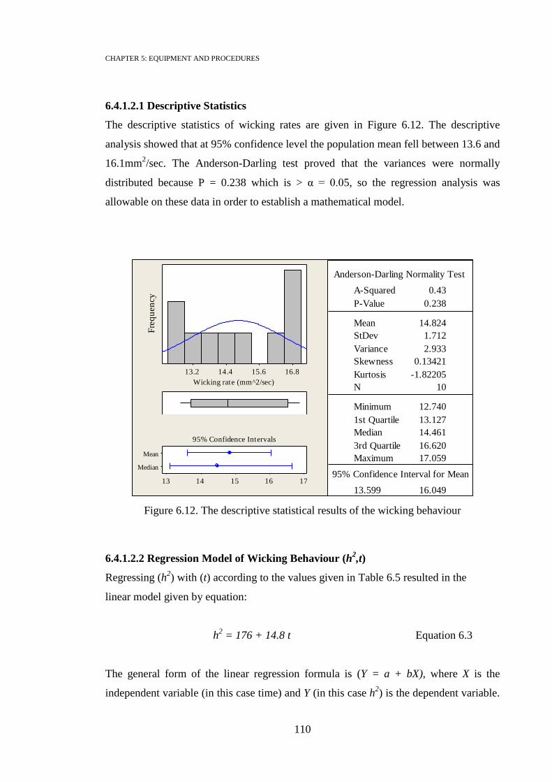
CHAPTER 5: EQUIPMENT AND PROCEDURES
110
6.4.1.2.1 Descriptive Statistics
The descriptive statistics of wicking rates are given in Figure 6.12. The descriptive
analysis showed that at 95% confidence level the population mean fell between 13.6 and
16.1mm2/sec. The Anderson-Darling test proved that the variances were normally
distributed because P = 0.238 which is > α = 0.05, so the regression analysis was
allowable on these data in order to establish a mathematical model.
Figure 6.12. The descriptive statistical results of the wicking behaviour
6.4.1.2.2 Regression Model of Wicking Behaviour (h2,t)
Regressing (h2) with (t) according to the values given in Table 6.5 resulted in the
linear model given by equation:
h2 = 176 + 14.8 t Equation 6.3
The general form of the linear regression formula is (Y = a + bX), where X is the
independent variable (in this case time) and Y (in this case h2) is the dependent variable.
16.815.614.413.2
Wicking rate (mm^2/sec)
Fre
qu
en
cy
Median
Mean
1716151413
1st Quartile 13.127
Median 14.461
3rd Quartile 16.620
Maximum 17.059
13.599 16.049
A-Squared 0.43
P-Value 0.238
Mean 14.824
StDev 1.712
Variance 2.933
Skewness 0.13421
Kurtosis -1.82205
N 10
Minimum 12.740
Anderson-Darling Normality Test
95% Confidence Interval for Mean
95% Confidence Interval for Median
95% Confidence Intervals

CHAPTER 5: EQUIPMENT AND PROCEDURES
111
The slope of the line is b = 14.8, and a = 176 is the intercept (i.e. the value of y when x
= 0).
This equation predicts at t = 0, h2
= 176, which is incorrect. Clearly the model is not
applicable when t = 0, because when t = 0 there is no wicking, but this value arose from
the regression model as the difference between the practical experiments and best fitting
line assumed by the regression analysis.
This model can be applied in case of capillary rise in an idealised tube, but in non-
homogenous materials such as textile fabrics, this modelling is not entirely correct. It
involves some error, because the relationship is not just between time and height; there
are other factors which play less important roles. For example, the viscosity of the
liquid, inertia and hydrostatic pressure are forces which affect the capillary rise.
Detailed Analysis
The detailed analysis of regression model (Table 6.7), proved that the intercept value
(176) and the wicking time (t) in the regression model were real effective values (did
not occur by chance) because the P-value was smaller than the pre-selected significance
level of this research (α = 0.05).
R-sq demonstrated that 99.6% of the variation in wicking rate was explained by the
regression model.
Table 6.7. Detailed analysis of the regression model
Predictor Coef SE Coef P
Constant 175.86 28.71 0.000
t 14.7932 0.1475 0.000
S = 108.39 R-Sq = 99.6% R-Sq(adj) = 99.6%
Analysis of Variance
The analysis of variance of the regression model (Table 6.8) indicated that the null
hypothesis (the independent variables do not affect the dependent) can be rejected
because P ≈ 0.000. Thereafter, the independent variable (t) had an effect on the
dependant variable (h2), giving confidence that the relationship was linear. Observation
(2) shown in Table 6.9 was identified as an unusual observation because its standardised
residual was less than -2. This could indicate that this observation is an outlier.
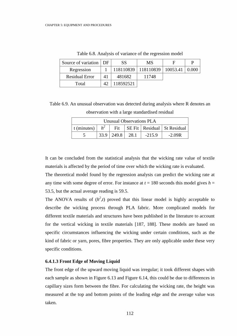
CHAPTER 5: EQUIPMENT AND PROCEDURES
112
Table 6.8. Analysis of variance of the regression model
Source of variation DF SS MS F P
Regression 1 118110839 118110839 10053.41 0.000
Residual Error 41 481682 11748
Total 42 118592521
Table 6.9. An unusual observation was detected during analysis where R denotes an
observation with a large standardised residual
Unusual Observations PLA
t (minutes) h2 Fit SE Fit Residual St Residual
5 33.9 249.8 28.1 -215.9 -2.09R
It can be concluded from the statistical analysis that the wicking rate value of textile
materials is affected by the period of time over which the wicking rate is evaluated.
The theoretical model found by the regression analysis can predict the wicking rate at
any time with some degree of error. For instance at t = 180 seconds this model gives h =
53.5, but the actual average reading is 59.5.
The ANOVA results of (h2,t) proved that this linear model is highly acceptable to
describe the wicking process through PLA fabric. More complicated models for
different textile materials and structures have been published in the literature to account
for the vertical wicking in textile materials [187, 188]. These models are based on
specific circumstances influencing the wicking under certain conditions, such as the
kind of fabric or yarn, pores, fibre properties. They are only applicable under these very
specific conditions.
6.4.1.3 Front Edge of Moving Liquid
The front edge of the upward moving liquid was irregular; it took different shapes with
each sample as shown in Figure 6.13 and Figure 6.14, this could be due to differences in
capillary sizes form between the fibre. For calculating the wicking rate, the height was
measured at the top and bottom points of the leading edge and the average value was
taken.

CHAPTER 5: EQUIPMENT AND PROCEDURES
113
Figure 6.13. Advancing liquid front sample 1 of PLA
Figure 6.14. Advancing liquid front sample 2 of PLA

CHAPTER 5: EQUIPMENT AND PROCEDURES
114
6.4.2 Dynamic Spreading of the Micro-Drop
This test aimed to characterise the PLA fabric properties in terms of micro drop
spreading. Dynamic spreading is another aspect of liquid transport in addition to vertical
wicking. It differs from vertical wicking because the liquid is transported in two
dimensions rather than in one dimension and moves horizontally. Therefore no
hydrostatic pressure is involved. Additionally, the first phase of spreading (before the
liquid penetrates into the fabric capillaries) occurs over the surface of fabric, therefore it
is strongly correlated with the surface characteristics of fabric which could be of benefit
in determining surface features, whereas in the case of vertical wicking the liquid moves
through the interior capillaries.
The spreading of a drop through a textile material is a complex process. The viscosity,
force of inertia and capillary forces effect the liquid movement during this transport. To
simplify the study, the force of inertia and viscosity was considered to have negligible
effect.
Note: details about the test background, methodology and procedure were provided in
Chapter 4 and Chapter 5.
6.4.2.1 Experiments and Results
Untreated PLA fabric was subjected to the drop spreading test. Ten trials were made
under the standard conditions of temperature 22°C and relative humidity 65%. In order
to understand the behaviour of drops spreading over the PLA fabric, the drop movement
was recorded from the moment of touch until the liquid transport become very slow
after around 900 seconds, as demonstrated in Figure 6.15.

CHAPTER 5: EQUIPMENT AND PROCEDURES
115
Figure 6.15. Demonstration of the spreading of micro drop
through PLA fabric
With reference to Equation 6.4 introduced by Kissa, explained in Section 4.6.2, the
relationship (A,t) was studied to examine the dynamic spreading behaviour.
Equation 6.4
The volume of the drop was 12.50 micro litres, and the coefficient (K), surface tension
(γ), and viscosity (η) were kept constant since the same liquid was used in all areas. The
area of the spreading droplet (A) was measured with time (t), starting from the smallest
possible area that was able to be detected. Ten trails were run, and then the average
values were obtained, which are presented in Table 6.10 along with the corresponding
logarithmic values used in analysis.
The scatter plot of the spreading process is shown in Figure 6.16. The images and
graphical analysis proved the spreading process consisted of two phases, in agreement
with the spreading review presented in Section 4.6. Phase I lasted about 1 second, whilst
phase II was a slow spreading process, extending until equilibrium was reached.

CHAPTER 5: EQUIPMENT AND PROCEDURES
116
Figure 6.17 shows the standard deviation of these ten trails associated with every
measured point. Generally the variation in spreading could be related to the deformable
nature of the knitted fabric, and the non-homogeneity of the fabric surface caused by
production processes and handling, or by further preparation processes such as sizing or
washing. The larger deviation found at the start of spreading process could be explained
by instantaneous impact when the drop touches the fabric and the inability of the camera
to constantly record the exact first touch moment with every new drop.
Table 6.10. Average values of spreading area measurements along with logarithmic
values
Time t (second) Area A (mm2) log t log A
0.00 0.00 - -
0.20 36.43 -0.70 1.56
0.40 50.97 -0.40 1.71
0.60 56.21 -0.22 1.75
0.80 60.10 -0.10 1.78
1.00 62.61 0.00 1.80
1.20 63.66 0.08 1.80
1.40 66.30 0.15 1.82
1.60 67.10 0.20 1.83
1.80 68.08 0.26 1.83
2.00 68.66 0.30 1.84
3.00 70.27 0.48 1.85
5.00 72.76 0.70 1.86
10.00 73.82 1.00 1.87
20.00 75.37 1.30 1.88
30.00 76.90 1.48 1.89
60.00 79.00 1.78 1.90
180.00 80.05 2.26 1.90
300.00 81.49 2.48 1.91
420.00 82.30 2.62 1.92
540.00 83.63 2.73 1.92
660.00 83.87 2.82 1.92
780.00 84.74 2.89 1.93
900.00 84.95 2.95 1.93
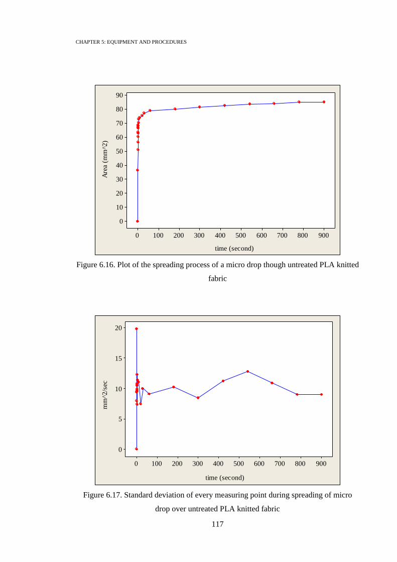
CHAPTER 5: EQUIPMENT AND PROCEDURES
117
Figure 6.16. Plot of the spreading process of a micro drop though untreated PLA knitted
fabric
Figure 6.17. Standard deviation of every measuring point during spreading of micro
drop over untreated PLA knitted fabric
9008007006005004003002001000
90
80
70
60
50
40
30
20
10
0
time (second)
Are
a (m
m^2
)
9008007006005004003002001000
20
15
10
5
0
time (second)
mm
^2/s
ec

CHAPTER 5: EQUIPMENT AND PROCEDURES
118
Figure 6.18 and Figure 6.19 display the logarithmic representation of the relationship
(log A, log t) and standard deviation respectively.
In correspondence with Equation 6.4, when all the other parameters are kept constant,
the relationship (log A, log t) is linear with slope (n). In practice the slope (n) expresses
the change in area of a drop with time; in other words it indicates the rate at which the
area increases with time, the higher the value of (n) the higher the rate. The following
analysis discusses the value of (n) as a quantitative measure for spreading process.
The analyses were done twice, for phase I and phase II. Table 6.11 gives the values of
the slopes (n) during both phases.
Figure 6.18. Logarithmic representation of the relation between area and time during
spreading
3210-1
1.95
1.90
1.85
1.80
1.75
1.70
1.65
1.60
1.55
log t
log
A
0
1.7919
phase I
phase II

CHAPTER 5: EQUIPMENT AND PROCEDURES
119
Figure 6.19. Standard deviation of logarithmic values of spreading area
Table 6.11. Values of slope (n) during first and second phase
A comparison of these results for PLA can be made with the results obtained by Kissa
and Kawase on permeable (cotton) and impermeable (polyester) fabrics, which were
reviewed and discussed in detail in Chapter 4. For the spreading of a 12.50 micro litre
3210-1
0.225
0.200
0.175
0.150
0.125
0.100
0.075
0.050
logt
log
A
0
phase I
phase II
replica Phase 1 replica Phase 2
n1 0.26 n2 0.03
n1 0.40 n2 0.03
n1 0.43 n2 0.02
n1 0.39 n2 0.03
n1 0.20 n2 0.03
n1 0.32 n2 0.03
n1 0.42 n2 0.03
n1 0.35 n2 0.03
n1 0.27 n2 0.03
n1 0.32 n2 0.04
average n1 0.34 average n2 0.037

CHAPTER 5: EQUIPMENT AND PROCEDURES
120
drop, the spreading rates n1 and n2 during phases I and II were 0.34 and 0.037
respectively, whereas Kawase that found for a drop volume range of 50 to 200 micro
litres n1 values of around 0.50 for impermeable and permeable fabrics during the phase
I, in contrast during phase II for impermeable fabrics, n2 = 0.30, but for permeable
fabrics n2 was subjective to the fabric properties, with some fabrics having values less
than 0.30 and others larger than 0.30. Another noticeable difference is that the first
phase (in the Kawase study) lasted about 5-6 seconds, while in this study the first phase
lasted only about 1 second.
In regard to the PLA study in this work, the considerably higher spreading rates of
phase I over phase II can be explained by the kinetic energy due to the drop impact
when it hits the fabric surface, in addition to the gravity and capillary forces available
for a larger amount of liquid to move. During phase II only the capillary force exists and
there is a smaller amount of free liquid still available to move.
6.4.2.2 Statistical Analysis of Spreading Rate of Untreated PLA
This is an attempt to find a mathematical model to clarify the spreading of micro
droplets through the PLA knitted fabric. The model depends on the assumption that the
spreading can be divided into two phases. In phase I the kinetic powers which push the
liquid are the gravity (liquid weight over the fabric surface) and capillary forces, while
in phase II only the capillary force acts.
The variables concerning phase I are referred to as t1 and A1, while for phase II they are
t2 and A2.
6.4.2.2.1 Descriptive Statistics of Untreated PLA Spreading Rate
Note: The definitions and explanation of the statistical terms were given in Chapter 5.
Phase I
The descriptive statistics displayed in Figure 6.20 describe the central tendency of data
by identifying the average (mean) and median of the n1 data. The population mean was
determined as between 0.29 and 0.38 at the 95% confidence level. Also the Anderson-
Darling normality test proved the data distribution was normal (P = 0.847 < α = 0.05),
therefore the data were permissible for regression analysis.

CHAPTER 5: EQUIPMENT AND PROCEDURES
121
Figure 6.20. Descriptive analysis of phase I
Phase II
Figure 6.21 displays the descriptive analysis of phase II. The mean n2 ≈ 0.03 was
smaller than the n1 ≈ 0.33 because there was a smaller amount of liquid during the
second phase as most of the liquid was used in first phase to fill the capillary spaces.
The population mean of the phase II (n2) was between 0.027 and 0.033. The Anderson-
Darling normality test proved the data were distributed normally (P = 0.776 < α = 0.05)
so it was permissible to apply regression analysis.
0.450.400.350.300.250.20
spreading rate (n1)
Fre
quency
Median
Mean
0.400.350.30
1st Quartile 0.27321
Median 0.33558
3rd Quartile 0.39596
Maximum 0.42993
0.28764 0.38352
A-Squared 0.20
P-Value 0.847
Mean 0.33558
StDev 0.07135
Variance 0.00509
Skewness -0.521036
Kurtosis -0.365150
N 11
Minimum 0.19941
Anderson-Darling Normality Test
95% Confidence Interval for Mean
95% Confidence Interval for Median
95% Confidence Intervals

CHAPTER 5: EQUIPMENT AND PROCEDURES
122
Figure 6.21. Descriptive statistics of phase II
6.4.2.2.2 Linear Regression Analysis of the (log A, log t) Relationship
Phase I
The graphical illustration of the (logA1, logt1) relationship shown in Figure 6.18
indicated this relation could be considered linear. The regression analysis suggested the
following model:
ln A1 = 1.81 + 0.34 ln t1 Equation 6.5
Detailed Analysis
The detailed analysis of the regression model shown in Table 6.12 proved that the
constant (1.81) and log t1 are real values, and did not rise by chance because P ≈ 0.00 <
α = 0.05. R-sq indicated that 95.9% of the variation can be explained by this model.
0.0360.0320.0280.024
spreading rate (n2)
Fre
quency
Median
Mean
0.03300.03150.03000.02850.0270
1st Quartile 0.027755
Median 0.029860
3rd Quartile 0.032268
Maximum 0.036255
0.027064 0.032656
A-Squared 0.22
P-Value 0.776
Mean 0.029860
StDev 0.004162
Variance 0.000017
Skewness -0.581430
Kurtosis 0.490240
N 11
Minimum 0.021421
Anderson-Darling Normality Test
95% Confidence Interval for Mean
95% Confidence Interval for Median
95% Confidence Intervals

CHAPTER 5: EQUIPMENT AND PROCEDURES
123
Table 6.12. Detailed analysis results
Predictor Coef SE Coef P
Constant 1.81351 0.01500 0.000
log t1 0.33441 0.03993 0.004
R-Sq = 95.9% R-Sq(adj) = 94.5%
Analysis of Variance
The analysis of variance results are presented in Table 6.13. The significant P ≈ 0.00 <
α = 0.05, therefore at 95% confidence the independent variable has an effect on the
dependant variable.
Table 6.13. Analysis of variance
Source DF SS MS F P
Regression 1 0.034074 0.034074 70.14 0.004
Residual Error 3 0.001457 0.000486
Total 4 0.035531
Equation 6.5 can be written as
Equation 6.6
This equation predicts that the area covered by the spreading liquid should increase with
time raised to power n1 = 0.34.
Phase II
Following the same steps applied to the phase I results, the relationship was found

CHAPTER 5: EQUIPMENT AND PROCEDURES
124
log A2 = 1.82 + 0.037 log t2 Equation 6.7
Detailed Analysis
Table 6.14 presents the detailed analysis of the regression model. The probability value
P for both the constant (1.82) and log t2 is less than 0.05; this proved that these values
did not occur by chance. R-sq stated that 96.3% of the variation can be explained by
Equation 6.7.
Table 6.14. Detailed analysis of phase II
Predictor Coef SE Coef P
Constant 1.82317 0.00330 0.000
log t2 0.036845 0.001814 0.000
R-Sq = 96.3% R-Sq(adj) = 96.0%
Analysis of Variance
The analysis of variance for the regression model presented in Table 6.15 demonstrated
that P ≈ 0.00 < 0.05, so there was 95% confidence of a strong linear relationship and
proved that the independent variable has an effect on the dependant variable. Table 6.16
shows one unusual point detected by the analysis of variance. It was associated with the
first reading in the second phase at t = 1.2 seconds.
Table 6.15. Analysis of variance
Source DF SS MS F P
Regression 1 0.028043 0.028043 412.47 0.000
Residual Error 16 0.001088 0.000068
Total 17 0.029131
Table 6.16. Unusual observation
Observation logt2 logA2 Fit SE Fit Residual St Residual
1 0.08 1.80385 0.00319 0.00319 -0.02224 -2.92R
R denotes on an observation with a large standardised residual

CHAPTER 5: EQUIPMENT AND PROCEDURES
125
Rearrangement of Equation 6.7 gave the following equation:
Equation 6.8
This equation predicts that the area covered by spreading liquid should increase with
time raised to power n2 = 0.037 during phase II.
6.4.2.3 The Dynamic Shape of Spreading Area
The dynamic change of the drop shape during spreading was studied because of its
importance in other textile process such as determining the quality of colour printing
[189]. In addition this feature was used to inspect the influence of the plasma and
enzyme preparations in distorting the liquid transport.
The roundness of the spreading area was estimated as a percentage of the ideal circular
area. The percentage factor (R) was calculated according to Equation 6.9, which was
given by the OLYMPUS Company, the provider of image analysis software
ANALYSIS 5. This equation expresses the roundness of the spreading area as a
percentage of the ideal circular area, as exemplified Figure 6.22.
Equation 6.9
Where M is the central moment
Figure 6.22. Schematic representation of expression of roundness

CHAPTER 5: EQUIPMENT AND PROCEDURES
126
Figure 6.23 and Figure 6.24 illustrate how the roundness according to Equation 6.9
changes with time during phases I and II respectively. The drop exhibited a roundness
of about 70% to 80% in the phase I. During phase II the drop tended to become more
circular in shape, with a roundness level of about 80% to 90%, possibly due to less
perturbation of liquid transport than the first phase where the impact of drop falling on
non-homogeneous knitted fabric surface is believed to affect the liquid movement.
Figure 6.23. Roundness change with time during phase I
1.00.80.60.40.20.0
1.0
0.8
0.6
0.4
0.2
0.0
time (second)
Ro
un
dn
ess
%
Phase I

CHAPTER 5: EQUIPMENT AND PROCEDURES
127
Figure 6.24. Roundness percentage during phase II
6.5 Dyeing of PLA
6.5.1 Disperse Dye
Disperse dyes were developed to dye acetate fibres first marketed in the 1920s, because
hydrophobic fibres have little affinity for water-soluble dyes. After polyester was
invented, new disperse dyes with better solubility in polyester were developed. These
dyes have much better solubility in polyester fibre than in water [190]. Disperse dyes
exist in the dye bath as a suspension or dispersion of microscopic particles, with only a
amount in true solution at any time. At the boil, or under pressure at even higher
temperatures, the small amount of dye soluble in water transfers by intermolecular force
to the fibre while more of the dispersed dye dissolved in the water. This process
continues until the dye is as fully transferred as possible from the dispersed state in
water to the dissolved state in the fibre. When cooled, the fibre structure tightens,
trapping the dye molecules, and resulting in excellent wet fastness properties.
Disperse dyes are usually applied to polyester at high temperature (> 130ºC) so dyeing
takes place above its glass transition temperature. Disperse dye molecules possess a
number of polar groups, like the nitro (-NO2), cyano (-CN), hydroxyl (-OH), substituted
amino (-NR1R2), ester (-COO-) amide (-NHCO-) and sulfone (-SO2-) groups. These
9008007006005004003002001000
1.0
0.8
0.6
0.4
0.2
0.0
time (second)
Ro
un
dn
ess
%
Phase II

CHAPTER 5: EQUIPMENT AND PROCEDURES
128
polar groups can make a number of contributions to the application properties of
disperse dyes. One of their roles is to provide an adequate degree of water solubility at
the high temperatures at which the dyes are applied. A second function of the polar
groups is to enhance affinity, as a result of dipolar intermolecular forces, with the ester
groups of the polyester molecule.
6.5.2 Exhaust Dyeing
The dyeing process of PLA was carried out by the exhaust dyeing method, using
Roaches-T infra-red machine. Exhaust dyeing is an important dyeing process. In this
process the dye molecules, dissolved or dispersed in a dye bath of moderately large
liquor to goods ratio, gradually leave the bath and attach to the fibres over a relatively
long period of time at elevated temperatures in machines. The dye is said to exhaust
from the dye-bath to the substrate. The ideal dye would exhaust totally, all the dye in
the dye bath would end up on the fibre. Exhaustion is sometimes specified as a
percentage. For example, 60% exhaustion would mean that 60% of the total amount of
dye has absorbed by the fibre, and 40% is still in the dye liquor.
6.5.3 Dyeing Procedure
Scouring
Prior to dyeing the fabric was scoured in a bath containing 1 g/l sodium carbonate
(Na2CO3) and 1 g/l Synperonic BD100 non-ionic detergent at 60 ºC for 15 minutes then
rinsed with cold water and finally rinsed with distilled water before drying at room
temperature.
Dyeing conditions
According to DyStar [191] the typical conditions for dyeing PLA with disperse dyes is
110ºC, for 30 - 45 minutes, at pH 4.5 - 5. The dyeing procedure utilised in this work is
displayed in Figure 6.25. The following parameters were selected to set a baseline for
comparing the colour yield with those obtained from the enzyme and plasma prepared
fabrics:
Dye shade 3%
Liquor to goods ratio 15:1
Disperse dye red B-2B C.I 60 200%

CHAPTER 5: EQUIPMENT AND PROCEDURES
129
110ºC for 45 min
1ºC/min 3ºC/min
Start at room temperature End at room temperature
Figure 6.25. Schematic representation of the dyeing process
6.5.4 Reduction Clearing
Reduction clearing is the removal of disperse dye on the surface of fabric by use of
reducing agent. Fine particles of disperse dye often remain on the surface of dyed fabric.
These particles can cause rubbing fastness problems, so they have to be removed by
reduction clearing to obtain the best fastness properties possible. After dyeing the fabric
was rinsed with warm water, then given alkaline reduction clearing in a bath containing
2 g/l sodium hydrosulphite (Na2O4S2) and 2 g/l sodium carbonate (Na2CO3) according
to the procedure given in Figure 6.26, then the sample was removed from the tube, and
rinsed at 40ºC in a solution of 1g/l Synperonic detergent and deionised water for 10
minutes, and then rinsed with water. The reductive clear was carried out using the same
machine as that for dyeing.
70ºC for 20 minutes
Heating as quickly as possible
Cooling to room temperature
Starts from room temperature
Figure 6.26. Schematic representation of reduction clearing process
6.5.5 Wash Fastness Test
Wash fastness for domestic laundering was determined according to the ISO 105:C06
test as presented in Table 6.17. The Gryowash machine was used for the test. A sample
of size 4 × 10 cm was attached to standard fabric. The wash liquor was prepared by

CHAPTER 5: EQUIPMENT AND PROCEDURES
130
dissolving ECE phosphate reference detergent and sodium preborate tetrahydrate and
heated to 50ºC. Then the wash liquor was added to the container together with the
sample and left for 30 min in the washing machine. After that the fabric was rinsed in
warm water. The fabric was assessed by comparing the K/S spectra, before and after the
wash fastness test.
Table 6.17. Wash fastness test parameters
Adjust pH
to
Steel
balls
Time
(min)
Sodium
Perborate
(g/l)
Available
chlorine
Liquor
volume
Temperature
(ºC)
Test
no.
Not
adjusted non 30 1 none 150 50 C06/B2S
6.5.6 Measurement of Visual Colour Yield (K/S)
The visual colour yield, expressed as K/S values, of the dyed substrate is defined by the
Kubelka-Munk equation (Equation 6.10)
K/S = (1-R) 2/2R Equation 6.10
Where K is the absorption constant at a given wavelength, S is the light scattering
constant, and R is the reflectance (as a fraction between 0 and 1.0)
The higher the K/S value, the greater is the colour intensity and hence, the better is the
dye uptake for given fabric and dye.
The spectral reflectance values (400-700 nm) were measured using a Spectra Flash
SF600 spectrophotometer (Datacolor International) using a 9.00 mm aperture.
The K/S curves of the dyed PLA fabric before and after wash fastness testing nearly
coincided, as shown in Figure 6.27. This indicated excellent wash fastness results as
very little change appeared on colour after the washing.

CHAPTER 5: EQUIPMENT AND PROCEDURES
131
Figure 6.27. K/S spectra of knitted PLA fabric
0
1
2
3
4
5
6
7
8
400 450 500 550 600 650 700 750
K/S
Wave length (nm)
PLA untreated disperse 3% before wash fastness test
PLA untreated disperse 3% after wash fastness test
CHAPTER 7: PREPARATION OF POLYLACTIC ACID AND POLYESTER FABRIC USING A EUROPLASMA CD400
MACHINE
132
Chapter 7
PREPARATION OF POLYLACTIC ACID AND POLYESTER FABRIC USING
A EUROPLASMA CD400 MACHINE
7.1 Introduction
Textile preparation processes using environmentally friendly plasma techniques can
modify the surface energy and topography of a polymer. Plasma treatment has a
complex effect, depending on the power, pressure and time; in other words the effect of
plasma treatment is a combination of the energy and flux of the excited species in the
plasma. Increasing the power will increase the intensity of the treatment, while
increasing the pressure will reduce the energy per active species, but will increase the
flux of these species on the surface of polymer. Decreasing the pressure will give more
energy to each molecule/atomic gas species, so may increase the etching effect,
although it will reduce the density of the bombarding species. The plasma species can
only sputter to a depth of about 1000 angstrom at the fibre surface [192].
This chapter is concerned with the study of preparation treatments of poly(lactic acid)
(PLA) and Polyester (PET) fabrics using the Europlasma CD400 machine introduced in
Chapter 5. Following the plasma treatment, the fabrics were subjected to a spreading
test to evaluate the effect of plasma treatment on the ability of the fabrics to transport
liquid. The techniques of X-ray Photoelectron Spectroscopy (XPS) and Scanning
Electron Microscopy (SEM) were utilised to examine the nature of the surface
modifications after the plasma treatment.
Note: details of all the equipment, machines and testing devices used in this study are
presented in Chapter 5.
7.2 Experimental Conditions
A low-temperature plasma machine Europlasma CD-400 was used, applying oxygen as
treatment gas. A wide range of experiments were conducted with the aim of modifying
the liquid transport properties of PLA and finding the optimum treatment conditions of
power, flux, and time. The polyester (PET) was used in this study as a reference fabric
to estimate the effectiveness of plasma treatment conditions and compare the results
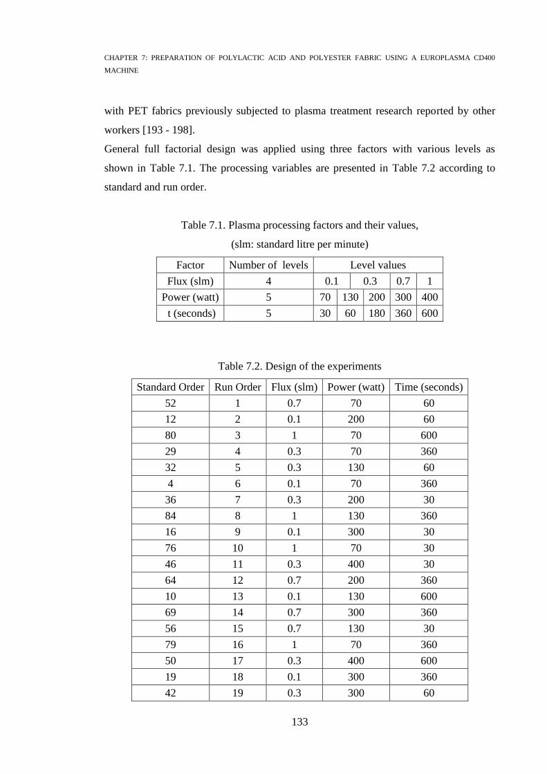
CHAPTER 7: PREPARATION OF POLYLACTIC ACID AND POLYESTER FABRIC USING A EUROPLASMA CD400
MACHINE
133
with PET fabrics previously subjected to plasma treatment research reported by other
workers [193 - 198].[193] [194] [195] [196] [197] [198].
General full factorial design was applied using three factors with various levels as
shown in Table 7.1. The processing variables are presented in Table 7.2 according to
standard and run order.
Table 7.1. Plasma processing factors and their values,
(slm: standard litre per minute)
Factor Number of levels Level values
Flux (slm) 4 0.1 0.3 0.7 1
Power (watt) 5 70 130 200 300 400
t (seconds) 5 30 60 180 360 600
Table 7.2. Design of the experiments
Standard Order Run Order Flux (slm) Power (watt) Time (seconds)
52 1 0.7 70 60
12 2 0.1 200 60
80 3 1 70 600
29 4 0.3 70 360
32 5 0.3 130 60
4 6 0.1 70 360
36 7 0.3 200 30
84 8 1 130 360
16 9 0.1 300 30
76 10 1 70 30
46 11 0.3 400 30
64 12 0.7 200 360
10 13 0.1 130 600
69 14 0.7 300 360
56 15 0.7 130 30
79 16 1 70 360
50 17 0.3 400 600
19 18 0.1 300 360
42 19 0.3 300 60

CHAPTER 7: PREPARATION OF POLYLACTIC ACID AND POLYESTER FABRIC USING A EUROPLASMA CD400
MACHINE
134
3 20 0.1 70 180
77 21 1 70 60
20 22 0.1 300 600
39 23 0.3 200 360
27 24 0.3 70 60
82 25 1 130 60
11 26 0.1 200 30
87 27 1 200 60
63 28 0.7 200 180
96 29 1 400 30
49 30 0.3 400 360
60 31 0.7 130 600
21 32 0.1 400 30
92 33 1 300 60
62 34 0.7 200 60
99 35 1 400 360
8 36 0.1 130 180
57 37 0.7 130 60
100 38 1 400 600
23 39 0.1 400 180
83 40 1 130 180
17 41 0.1 300 60
95 42 1 300 600
54 43 0.7 70 360
93 44 1 300 180
41 45 0.3 300 30
53 46 0.7 70 180
91 47 1 300 30
37 48 0.3 200 60
22 49 0.1 400 60
78 50 1 70 180
85 51 1 130 600
98 52 1 400 180
88 53 1 200 180
65 54 0.7 200 600
68 55 0.7 300 180
25 56 0.1 400 600

CHAPTER 7: PREPARATION OF POLYLACTIC ACID AND POLYESTER FABRIC USING A EUROPLASMA CD400
MACHINE
135
58 57 0.7 130 180
73 58 0.7 400 180
55 59 0.7 70 600
48 60 0.3 400 180
14 61 0.1 200 360
2 62 0.1 70 60
70 63 0.7 300 600
43 64 0.3 300 180
30 65 0.3 70 600
40 66 0.3 200 600
34 67 0.3 130 360
81 68 1 130 30
45 69 0.3 300 600
74 70 0.7 400 360
71 71 0.7 400 30
6 72 0.1 130 30
66 73 0.7 300 30
35 74 0.3 130 600
24 75 0.1 400 360
33 76 0.3 130 180
31 77 0.3 130 30
1 78 0.1 70 30
13 79 0.1 200 180
61 80 0.7 200 30
7 81 0.1 130 60
51 82 0.7 70 30
59 83 0.7 130 360
47 84 0.3 400 60
90 85 1 200 600
75 86 0.7 400 600
94 87 1 300 360
38 88 0.3 200 180
26 89 0.3 70 30
67 90 0.7 300 60
15 91 0.1 200 600
89 92 1 200 360
9 93 0.1 130 360
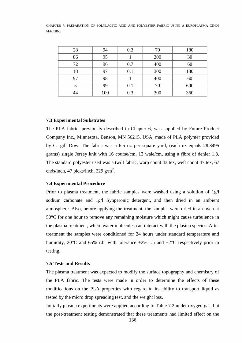
CHAPTER 7: PREPARATION OF POLYLACTIC ACID AND POLYESTER FABRIC USING A EUROPLASMA CD400
MACHINE
136
28 94 0.3 70 180
86 95 1 200 30
72 96 0.7 400 60
18 97 0.1 300 180
97 98 1 400 60
5 99 0.1 70 600
44 100 0.3 300 360
7.3 Experimental Substrates
The PLA fabric, previously described in Chapter 6, was supplied by Future Product
Company Inc., Minnesota, Benson, MN 56215, USA, made of PLA polymer provided
by Cargill Dow. The fabric was a 6.5 oz per square yard, (each oz equals 28.3495
grams) single Jersey knit with 16 course/cm, 12 wale/cm, using a fibre of denier 1.3.
The standard polyester used was a twill fabric, warp count 43 tex, weft count 47 tex, 67
ends/inch, 47 picks/inch, 229 g/m2.
7.4 Experimental Procedure
Prior to plasma treatment, the fabric samples were washed using a solution of 1g/l
sodium carbonate and 1g/l Synperonic detergent, and then dried in an ambient
atmosphere. Also, before applying the treatment, the samples were dried in an oven at
50°C for one hour to remove any remaining moisture which might cause turbulence in
the plasma treatment, where water molecules can interact with the plasma species. After
treatment the samples were conditioned for 24 hours under standard temperature and
humidity, 20°C and 65% r.h. with tolerance ±2% r.h and ±2°C respectively prior to
testing.
7.5 Tests and Results
The plasma treatment was expected to modify the surface topography and chemistry of
the PLA fabric. The tests were made in order to determine the effects of these
modifications on the PLA properties with regard to its ability to transport liquid as
tested by the micro drop spreading test, and the weight loss.
Initially plasma experiments were applied according to Table 7.2 under oxygen gas, but
the post-treatment testing demonstrated that these treatments had limited effect on the

CHAPTER 7: PREPARATION OF POLYLACTIC ACID AND POLYESTER FABRIC USING A EUROPLASMA CD400
MACHINE
137
PLA fabric. Generally the treated substrates were characterised by similar features in
terms of the spreading rates and surface chemical features. These features proved to be
slightly different from the untreated fabric, as explained in the following sections.
Therefore it was decided to present only the results which exhibited most pronounced
effects on PLA fabric.
7.5.1 Weight Loss Assessment
It is normal for a fabric to lose some weight during plasma treatment, which is usually
attributed to physical etching. PLA polymer consists of crystalline and amorphous
regions, therefore the etching would be selective and more severe at the amorphous
regions because they are softer and easily attacked [199].
The fabric weight loss was calculated by weighing the fabric sample before treatment
W1, and after treatment W2, the fractional weight loss W is estimated as percentage %.
Equation 7.1
Five fabric samples of the same original weight (4 g) were treated, and the average
weight loss was taken. The loss in weight appeared to be minor, for example samples of
4.00 g became 3.92 g after treatment at maximum etching.
Figure 7.1 shows the weight loss after different treatment times of oxygen plasma. It
appeared that with increasing the time more etching occurred. A longer treatment time
may provide an opportunity for the plasma species to penetrate into the interior region
of the material, but the prolonged treatment damaged the fabric, as the sample turned
yellowish and gave a burning smell. Figure 7.2 illustrates the influence of power in the
machine, using oxygen plasma, on weight loss. With increasing power, the energy per
active species increases, therefore the weight loss becomes more pronounced.
On the other hand, increase in the gas flux caused less effect on weight loss than
increasing the time or power, as shown in Figure 7.3, because increasing the flux
reduces the energy per active species.

CHAPTER 7: PREPARATION OF POLYLACTIC ACID AND POLYESTER FABRIC USING A EUROPLASMA CD400
MACHINE
138
Figure 7.1. Weight loss under various durations
Treatment conditions: power = 200 watt, flux = 0.7 slm
Figure 7.2. Weight loss under various power levels
Treatment conditions: time = 5 minutes, flux = 0.7 slm
0
0.5
1
1.5
2
2.5
0 100 200 300 400 500 600 700
W %
Time (seconds)
0
0.2
0.4
0.6
0.8
1
1.2
1.4
0 100 200 300 400 500
W%
Power (watt)

CHAPTER 7: PREPARATION OF POLYLACTIC ACID AND POLYESTER FABRIC USING A EUROPLASMA CD400
MACHINE
139
Figure 7.3. Weight loss under different flux
Treatment conditions: time = 5 minutes, power = 200 watts
7.5.2 Surface Topography Analysis by Scanning Electron Microscopy (SEM)
Although a wide range of plasma processing conditions were applied on PLA fabric
according to Table 7.2, the topographical modification was limited. The overall effect
can be described by some micro-pitting or scars appearing on the treated area. The scars
appeared in some places on the surface and were unevenly distributed.
Hitachi S-4300 SEM was used for surface analysis of the fibre surface. The SEM image
given in Figure 7.4 illustrates the surface appearance of an untreated sample. As can be
seen, it is smooth with some blisters made by the production processes. On the other
hand, for example of the effect of oxygen plasma treatment under the condition “200
watt, 0.7 slm, 5 minutes” shown in Figure 7.5, some etching can be observed on the
surface.
In regard to the reference fabric (polyester), under the same previously mentioned
conditions, the SEM scan revealed random etching occurring after plasma treatment.
The SEM micrographs shown in Figure 7.6 and Figure 7.7 provide visual comparison of
PET before and after plasma treatment.
0.00
0.20
0.40
0.60
0.80
1.00
1.20
0 0.2 0.4 0.6 0.8 1 1.2
W %
Flux (slm)

CHAPTER 7: PREPARATION OF POLYLACTIC ACID AND POLYESTER FABRIC USING A EUROPLASMA CD400
MACHINE
140
Figure 7.4. SEM micrographs of untreated PLA fabric
Figure 7.5. SEM images of PLA fibre after plasma treatment
Treatment conditions: 200 watt, 0.7 slm, 5 minutes

CHAPTER 7: PREPARATION OF POLYLACTIC ACID AND POLYESTER FABRIC USING A EUROPLASMA CD400
MACHINE
141
Figure 7.6. SEM images of untreated polyester fabric
Figure 7.7. SEM images of PET fibres after plasma treatment

CHAPTER 7: PREPARATION OF POLYLACTIC ACID AND POLYESTER FABRIC USING A EUROPLASMA CD400
MACHINE
142
7.5.3 Chemical Composition Analysis by X-ray Photoelectron Microscopy (XPS)
Samples treated in oxygen plasma at 200 watt, 0.7 slm, for 5 minutes were studied and
analysed by XPS. The scan was performed five days after the oxygen plasma treatment.
Three batches were treated and analysed by XPS, then average measurement were
taken.
The survey scans of untreated and treated samples are illustrated in Figure 7.8 and
Figure 7.9. Both graphs exhibited two main peaks, C1s at 286.4 eV and O1s at 532.5
eV. Though there is a difference in counts per second between the untreated and treated
samples, this difference is due to variations in sample alignment and beam intensity.
The samples cannot be compared based upon the absolute counts per second.
The detailed C1s spectra of both untreated and treated PLA are shown in Figure 7.10
and Figure 7.11 respectively. There were no major differences detected on the surfaces
between the treated and untreated samples and the relative chemical composition was
very similar to the untreated percentage given in Chapter 6 (Table 6.2). This suggests
that preparation process of PLA fabric utilising the Europlasma CD400 machine did not
produce new chemical groups on the polymer surface.
In contrast to the PLA response to treatment conditions, new functional groups were
introduced on the surface of the PET fibres. The survey scans of PET before and after
treatment are shown in Figure 7.12 and Figure 7.13 respectively. Two main peaks
appeared in the survey scan related to C1s at 285 eV and O1s at 533 eV.
The C1s spectrum of untreated PET consists mainly of three distinct peaks. They
correspond to the carbon atoms in the phenyl ring (C-C or C-H) at (284.66 eV), the
alkyl chain (C-O) carbon singly bonded to oxygen at (286.18 eV) and the ester carbon
atoms (O-C=O) at (288.72 eV) [200]. Post plasma treatment, the C1s spectrum of PET
showed the presence of new carbonyl (C=O) groups at 287.87 eV. This confirms the
formation of a new polar group after oxygen plasma treatment and explains the increase
in spreading rate. The new C=O group formed on the PET surface after plasma
treatment was made at the expense of C-C, C-H, C-O bonds as shown in Table 7.3 and
Table 7.4.

CHAPTER 7: PREPARATION OF POLYLACTIC ACID AND POLYESTER FABRIC USING A EUROPLASMA CD400
MACHINE
143
Figure 7.8. Survey scan of untreated PLA sample
Figure 7.9. Survey scan of treated PLA sample
0
10000
20000
30000
40000
50000
60000
70000
80000
90000
0 200 400 600 800 1000 1200 1400
count
per
sec
ond
BE (eV)
survey scan for untreated PLA sample
C1s
O1s
0
10000
20000
30000
40000
50000
60000
0 200 400 600 800 1000 1200 1400
count
per
sec
ond
BE (eV)
survey scan after treatment
C1s
O1s

CHAPTER 7: PREPARATION OF POLYLACTIC ACID AND POLYESTER FABRIC USING A EUROPLASMA CD400
MACHINE
144
Figure 7.10. XPS C1s spectrum of untreated PLA sample
Figure 7.11. XPS C1s spectrum of treated PLA sample
0
1000
2000
3000
4000
5000
6000
7000
275 280 285 290 295 300 305
count
per
sec
ond
BE (eV)
C1s Spectra of untreated PLA
C 1s:CPS
C 1s:C 1s
C 1s:C 1s
C 1s:C 1s
0
1000
2000
3000
4000
5000
6000
275 280 285 290 295 300 305
coun
t per
sec
on
d
BE (eV)
C1s Spectrum of PLA after treatment
C 1s:CPS
C 1s:C 1s
C 1s:C 1s
C 1s:C 1s

CHAPTER 7: PREPARATION OF POLYLACTIC ACID AND POLYESTER FABRIC USING A EUROPLASMA CD400
MACHINE
145
Figure 7.12. XPS survey scan of untreated PET
Figure 7.13. XPS survey scan of plasma treated PET
0
10000
20000
30000
40000
50000
60000
0 200 400 600 800 1000 1200 1400
count
per
sec
ond
BE (eV)
survey scan of untreated PET
O1s
C1s
0
10000
20000
30000
40000
50000
60000
70000
0 200 400 600 800 1000 1200 1400
cou
nt
per
sec
ond
BE (eV)
survey scan of treated PET
O1s
C1s

CHAPTER 7: PREPARATION OF POLYLACTIC ACID AND POLYESTER FABRIC USING A EUROPLASMA CD400
MACHINE
146
Figure 7.14. C1s spectra of untreated PET
Figure 7.15. C1s spectra of treated PET
0
2000
4000
6000
8000
10000
12000
275 280 285 290 295 300 305
Count
per
sec
ond
BE (eV)
C 1s:CPS
C 1s:C 1s
C 1s:C 1s
C 1s:C 1s
0
1000
2000
3000
4000
5000
6000
7000
8000
9000
275 280 285 290 295 300 305
count
per
sec
ond
BE (eV)
C1s spectra of treated PET
C 1s:CPS
C 1s:C 1s
C 1s:C 1s
C 1s:C 1s
C 1s:C 1s
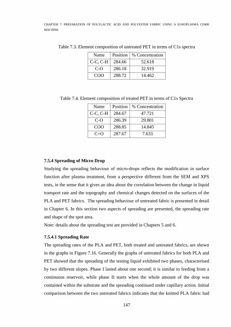
CHAPTER 7: PREPARATION OF POLYLACTIC ACID AND POLYESTER FABRIC USING A EUROPLASMA CD400
MACHINE
147
Table 7.3. Element composition of untreated PET in terms of C1s spectra
Name Position % Concentration
C-C, C-H 284.66 52.618
C-O 286.18 32.919
COO 288.72 14.462
Table 7.4. Element composition of treated PET in terms of C1s Spectra
Name Position % Concentration
C-C, C-H 284.67 47.721
C-O 286.39 29.801
COO 288.85 14.845
C=O 287.67 7.633
7.5.4 Spreading of Micro Drop
Studying the spreading behaviour of micro-drops reflects the modification in surface
function after plasma treatment, from a perspective different from the SEM and XPS
tests, in the sense that it gives an idea about the correlation between the change in liquid
transport rate and the topography and chemical changes detected on the surfaces of the
PLA and PET fabrics. The spreading behaviour of untreated fabric is presented in detail
in Chapter 6. In this section two aspects of spreading are presented, the spreading rate
and shape of the spot area.
Note: details about the spreading test are provided in Chapters 5 and 6.
7.5.4.1 Spreading Rate
The spreading rates of the PLA and PET, both treated and untreated fabrics, are shown
in the graphs in Figure 7.16. Generally the graphs of untreated fabrics for both PLA and
PET showed that the spreading of the testing liquid exhibited two phases, characterised
by two different slopes. Phase I lasted about one second; it is similar to feeding from a
continuous reservoir, while phase II starts when the whole amount of the drop was
contained within the substrate and the spreading continued under capillary action. Initial
comparison between the two untreated fabrics indicates that the knitted PLA fabric had

CHAPTER 7: PREPARATION OF POLYLACTIC ACID AND POLYESTER FABRIC USING A EUROPLASMA CD400
MACHINE
148
higher spreading rate than woven PET fabric. Apart from the effect of fabric structure
on the spreading process, this spreading behaviour agreed with already reported
properties about PLA and PET; that PLA has lower contact angle and higher wicking
rate, which was previously mentioned in Section 2.5.3.
Figure 7.16. Spreading behaviour of micro drop through PLA and PET before and after
oxygen plasma treatment
Treatment conditions: 5 min, 0.7 slm, 200 watt
Post plasma treatment, the PLA and PET samples exhibited quite different responses to
spreading. With regard to PLA, the first phase of the treated fabric lasted longer (about
2 seconds) than for the untreated fabric (about one second). The spot area of the second
phase of the treated fabric increased gradually and slowly until it equalled that of the
untreated fabric at around 900 seconds. The status of the first phase is probably
correlated with influence of roughness on contact angle, as the roughness could increase
the contact angle as explained in Section 4.2.4, consequently this could be expected to
delay the droplet being contained by the fabric. During the second phase, the spreading
0
20
40
60
80
100
120
140
160
180
0 200 400 600 800 1000
Are
a (m
m^2)
Time (second)
PLA untreated
PLA treated
PET untreated
PET treated

CHAPTER 7: PREPARATION OF POLYLACTIC ACID AND POLYESTER FABRIC USING A EUROPLASMA CD400
MACHINE
149
process continues through pores between fibres, which should not have been effected by
plasma etching, as plasma etching usually occurs on the outermost surface layers.
Also it was observed that the spreading behaviour of treated PLA exhibited greater
variation than untreated PLA, in particular during the first phase, as demonstrated in
Figure 7.17. This could be explained by a heterogeneous surface roughness, created by
the uneven etching which appeared in the SEM micrographs.
Figure 7.17. Initial spreading of droplet on PLA during first 60 seconds
The images in Figure 7.18 and Figure 7.19 show the spreading of micro-drops on
untreated and treated PLA fabrics respectively. The images of the treated PLA fabric
demonstrated the delay in drop penetration into the fabric; this could be a consequence
of the increase in roughness of the fibres due to the etching action which was verified by
the SEM images.
0
10
20
30
40
50
60
70
80
90
0 10 20 30 40 50 60 70
Are
a (m
m^2)
Time (seconds)
PLA untreated
PLA treated
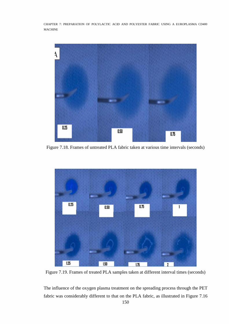
CHAPTER 7: PREPARATION OF POLYLACTIC ACID AND POLYESTER FABRIC USING A EUROPLASMA CD400
MACHINE
150
Figure 7.18. Frames of untreated PLA fabric taken at various time intervals (seconds)
Figure 7.19. Frames of treated PLA samples taken at different interval times (seconds)
The influence of the oxygen plasma treatment on the spreading process through the PET
fabric was considerably different to that on the PLA fabric, as illustrated in Figure 7.16

CHAPTER 7: PREPARATION OF POLYLACTIC ACID AND POLYESTER FABRIC USING A EUROPLASMA CD400
MACHINE
151
and Figure 7.20. Mainly the difference appeared in larger spreading and less variation
than for the PLA.
Two phases existed; the first phase lasted about 1 second, characterised by an instant
large increase in the spot area from the moment of touch until all the liquid was
contained within the fabric, while the second phase lasted until the equilibrium was
reached. The large spreading area of PET achieved after plasma treatment could be
related to the introduction of the new polar group (C=O), as explained previously in the
XPS data analysis.
Figure 7.20. Spreading rates on PET woven fabric during first 60 seconds
The images in Figure 7.21 and Figure 7.22 demonstrate the spreading process on
untreated and treated PET fabric respectively. Generally in both situations, the spot area
took a longitudinal shape in the direction of the warp, in contrast to the more circular
shape on the knitted PLA. Also fingering patterns (spreading of liquid in irregular
manner along individual yarns) were noticeable on the spot area of the woven PET
fabric.
0
20
40
60
80
100
120
140
0 20 40 60 80
Are
a (m
m^2)
Time (seconds)
PET untreated
PET treated

CHAPTER 7: PREPARATION OF POLYLACTIC ACID AND POLYESTER FABRIC USING A EUROPLASMA CD400
MACHINE
152
Figure 7.21. Frames of untreated PET samples, showing the spreading at different time
intervals (seconds)
Figure 7.22. Frames of treated PET samples, showing the spreading at different time
intervals (seconds)
A

CHAPTER 7: PREPARATION OF POLYLACTIC ACID AND POLYESTER FABRIC USING A EUROPLASMA CD400
MACHINE
153
7.5.4.2 Numerical Analysis of Spreading Results
According to the theoretical review presented in Chapter 4, the logarithmic relation (log
A, log t) is expected to be linear with slope n, which refers to the rate of area growing or
the rate of change over time. The higher the value of n, the faster the rate changes. It
may be that the n value is lower or higher than that for another sample, but the whole
graph could be at completely different level. This depends on the first spot area depicted
and recorded on the camera. Therefore along with comparing the n value, the first spot
area depicted on the camera should be taken in the consideration.
The logarithmic plots shown in Figure 7.23, either for PLA or PET, describe
approximately linear relations between log A and log t. The values of the slopes n before
and after treatment are presented in Table 7.5 for both PLA and PET.
In regard to PLA the values of slopes n1 and n2 after treatment are higher than those n1
and n2 before treatment, but the wetted area of the untreated fabric is larger than that of
the treated fabric after the same time. The steeper incline of the lines of treated samples
can be related to increase in roughness, which helped to hold the liquid for a longer time
over the fabric. In addition to this, the etching could remove the amorphous regions
from the fabric surface, which are responsible for absorbing part of the free liquid. So
the overall result is for more free liquid to be available to move, leading to a steeper
incline and higher n value.
In regard to PET, after treatment the slopes n1 and n2 are smaller than before treatment.
This could be explained by the increase in hydrophilicity due to the presence of the new
polar group (C=O) on the fabric after the plasma treatment. These new hydrophilic
groups caused immediate spreading, so the liquid instantly spread over a larger area
when it touched the fabric. The first spot area detected by camera was quite large in
comparison to untreated one, thereafter the amount of free liquid became small and led
to a less steep incline in the line than for the untreated fabric.

CHAPTER 7: PREPARATION OF POLYLACTIC ACID AND POLYESTER FABRIC USING A EUROPLASMA CD400
MACHINE
154
Figure 7.23. Logarithmic representation of spreading rates of PET and PLA
Table 7.5. Values of the slope n before and after plasma treatment
slope PLA PET
untreated treated untreated treated
Phase I 0.34 0.65 0.9 0.3
Phase II 0.03 0.06 0.08 0.10
7.5.4.3 The Dynamic Change of Stain Shape
In addition to examining the rate of spreading, the stain shape is considered another
important factor in the spreading of micro drops. The treatment, which may improve the
spreading rate, could cause shape distortion. In processes such as inkjet printing, drop
distortion is an important element in determining the image quality.
The shape of the drop was studied by estimating roundness factor, R, of the spreading
area, according to Equation 6.9.
The dynamic change of stain shape during spreading was assessed for both PET and
PLA before and after the plasma treatment. The changes in roundness of the spreading
liquid areas with time are demonstrated in Figure 7.24. The knitted untreated PLA
exhibited a higher level of roundness consistency during spreading than the untreated
0
0.5
1
1.5
2
2.5
-1 0 1 2 3 4
log A
log t
PLA untreated
PLA treated
PET untreated
PET treated

CHAPTER 7: PREPARATION OF POLYLACTIC ACID AND POLYESTER FABRIC USING A EUROPLASMA CD400
MACHINE
155
woven PET. However the shapes on the treated samples were less round in each case,
which could be related to irregularity of the plasma etching, as the plasma can etch the
amorphous regions more than the crystalline regions.
Woven PET exhibited a sharp decrease in roundness during spreading, the liquid
moving in a longitudinal shape, in the direction of the warp, and showing fingering
patterns. The final spot shape of treated and untreated PET fabric exhibited the same
level of roundness.
Figure 7.24. Roundness of the spreading areas of liquids
0.00
0.20
0.40
0.60
0.80
1.00
1.20
0 500 1000 1500 2000
Roundnes
s %
Time (second)
PLA untreated
PLA treated
PET untreated
PET treated

CHAPTER 8: PREPARATION OF POLYLACTIC ACID FABRIC USING THE NANOTECH PE250 PLASMA MACHINE
156
Chapter 8
PREPARATION OF POLYLACTIC ACID FABRIC USING THE NANOTECH
PE250 PLASMA MACHINE
Chapter Overview
The preparation of PLA using the Nanotech PE250 machine was conducted following
the study presented in Chapter 7 using the Europlasma machine, in an attempt to view
the previous results in proper perspective by comparing the abilities of two machines of
the same type (low pressure plasma) but with different designs.
This chapter presents the effect of twelve different preparation conditions on the
wicking and spreading behaviours of PLA fabric. The results were analysed statistically,
and the interpretation of outcome was made through the SEM micrographs and XPS
data.
Notes:
Information about the Nanotech PE250 plasma machine was provided in
Chapter 5.
The time was used in two different contexts. The time taken for the liquid to
wick though the fabric was coded (t) whereas the time of the treatment inside the
plasma chamber was coded (T).
Details of the statistical terms used in this chapter are given in Chapter 5.
The design of the experiment and the analyses were run using Minitab 15.1
8.1 Design of the Experiments
A general full factorial design was created, based on the three factors at the different
levels shown in Table 8.1.
The experiments and results are presented in this chapter according to the standard order
given in Table 8.2. However the experiments were applied randomly according to the
randomised order displayed in Table 8.3. In order to lessen the effects of factors that
were not included in the study, such as the variation due to instability of temperature
and humidity during conditioning, or the variation because of the possible deformation
of the knitted fabric. Prior to the plasma treatment, samples were washed using a

CHAPTER 8: PREPARATION OF POLYLACTIC ACID FABRIC USING THE NANOTECH PE250 PLASMA MACHINE
157
solution of deionised water with sodium carbonate (1g/l) and synperonic detergent
(1g/l) to remove any contamination from previous processes and then dried in an
ambient atmosphere. After subjecting the substrates to plasma treatment, they were
conditioned for 24 hours under standard conditions of humidity and temperature 65% ±
2% r.h, and 20 ± 2°C respectively, then the plasma treated samples were evaluated in
terms of modifications in vertical wicking and spreading of micro-drops, as described in
Chapter 5.
Table 8.1. Process parameters, “mbar = 100Pa”
Factor Number of levels Level values
Pressure (mbar) 2 0.5 1.5
Power (watts) 2 25 50
T (minute) 3 1 3 5
Table 8.2. Standard order of the treatment sets
Experiment code Pressure (mbar) Power (watts) Time (min)
1 0.5 25 1
2 0.5 25 3
3 0.5 25 5
4 0.5 50 1
5 0.5 50 3
6 0.5 50 5
7 1.5 25 1
8 1.5 25 3
9 1.5 25 5
10 1.5 50 1
11 1.5 50 3
12 1.5 50 5

CHAPTER 8: PREPARATION OF POLYLACTIC ACID FABRIC USING THE NANOTECH PE250 PLASMA MACHINE
158
Table 8.3. Randomisation Order of the experiments
Run Order Pressure (mbar) Power (watts) t (minute)
1 0.5 25 1
2 1.5 50 1
3 1.5 25 1
4 0.5 50 3
5 1.5 25 3
6 0.5 50 5
7 0.5 50 1
8 0.5 25 3
9 1.5 25 5
10 0.5 25 5
11 1.5 50 5
12 1.5 50 3
8.2 Vertical Wicking Test
The test was carried out according to the previously introduced procedure in Chapter 5
and Chapter 6. The wicking rate was calculated during the first 360 seconds of wicking
in accordance with the discussion stated in Section 6.6.
8.2.1 Experimental Results
Table 8.4 illustrates the wicking rates of fabric treated under various conditions. Each
experimental set was repeated five times. Figure 8.1 demonstrates the relationship
between time (t) and the wicking height (h) during first 360 seconds. This relationship
between wicking height and time is presented as (h2,t) in Figure 8.2, in reference to
Washburn equation explained in Chapter 4 and the methodology given in Chapter 5.
Most of the plots exhibited a high degree of linearity.

CHAPTER 8: PREPARATION OF POLYLACTIC ACID FABRIC USING THE NANOTECH PE250 PLASMA MACHINE
159
Table 8.4. Wicking rate after plasma treatment where R refers to repeat
Experiment Wicking rate replicates (mm
2/sec)
Average mm2/sec
R1 R2 R3 R4 R5
1 19.83 17.84 18.72 18.77 17.35 18.50
2 18.10 14.70 15.65 14.69 17.23 16.07
3 16.46 17.07 16.72 16.94 17.47 16.93
4 18.48 30.26 27.92 26.58 28.02 26.25
5 32.33 32.41 32.27 30.70 31.16 31.77
6 33.38 32.20 31.77 17.10 31.50 29.19
7 18.69 16.82 15.08 18.04 18.05 17.34
8 28.57 26.92 29.48 29.11 28.33 24.48
9 25.50 27.38 23.81 26.89 25.54 21.82
10 32.06 32.17 31.88 29.34 23.30 29.75
11 30.33 30.51 27.10 30.07 31.84 29.97
12 24.49 25.63 28.41 31.18 25.96 27.13
Figure 8.1. Graphical representation of (h,t) relationship after plasma treatment, where
C refers to control (untreated samples)
4003002001000
120
100
80
60
40
20
0
time (second)
hei
gh
t (m
m)
10
11
12
C
1
2
3
4
5
6
7
8
9
Untreated PLA

CHAPTER 8: PREPARATION OF POLYLACTIC ACID FABRIC USING THE NANOTECH PE250 PLASMA MACHINE
160
Figure 8.2. Experimental results of wicking rate (h2,t) graph,
C refers to untreated PLA
8.2.2 Statistical Analysis
The results were analysed and compared with the untreated sample that was studied in
Chapter 6.
The following studies investigated how different treatment conditions influenced the
wicking rate. The analyses utilised various statistical approaches, including Levene
tests, regression models, standard deviation, and box blots, to generate an overall view
about the treatment.
Although some treatment sets could achieve higher wicking rates, they exhibited higher
levels of variation. The statistical analyses clarified the working conditions for
generating optimum wicking rates.
8.2.2.1 Descriptive Analysis of Wicking Rates
Graphical and numerical summaries of the descriptive statistics for twelve treated
samples are displayed in the Figures below. The descriptive statistics provided
comprehensive information on the central tendency of the data values such as mean and
4003002001000
12000
10000
8000
6000
4000
2000
0
time (second)
h^2
(m
m)
10
11
12
C
1
2
3
4
5
6
7
8
9
Untreated PLA

CHAPTER 8: PREPARATION OF POLYLACTIC ACID FABRIC USING THE NANOTECH PE250 PLASMA MACHINE
161
median, and the spread of data by giving the standard deviation and interquartile range.
The histograms show the relative frequency each value occurred.
In comparison to the untreated sample which had a wicking rate of 14.82 mm2/sec,
treatment condition number (5) achieved the highest wicking rate while treatment
condition number (2) achieved the least improvement. The Anderson-Darling normality
tests demonstrated that the results of all twelve treatment conditions were normally
distributed since P = 0.238 > α = 0.0.5, therefore they were subjected to regression
modelling.
Figure 8.3. Descriptive statistics for the wicking rate for sample (1)
treated under (0.5 mbar, 25 watts, 1 min)
20.019.519.018.518.017.5
1.00
0.75
0.50
0.25
0.00
wicking rate (mm^2/sec)
Rela
tiv
e f
req
uen
cy
Median
Mean
20.019.519.018.518.017.517.0
1st Quartile 17.595
Median 18.720
3rd Quartile 19.302
Maximum 19.832
17.316 19.690
17.350 19.832
0.573 2.747
A-Squared 0.22
P-Value 0.667
Mean 18.503
StDev 0.956
Variance 0.914
Skewness 0.266859
Kurtosis -0.379139
N 5
Minimum 17.350
Anderson-Darling Normality Test
95% Confidence Interval for Mean
95% Confidence Interval for Median
95% Confidence Interval for StDev
95% Confidence Intervals
Summary for 1

CHAPTER 8: PREPARATION OF POLYLACTIC ACID FABRIC USING THE NANOTECH PE250 PLASMA MACHINE
162
Figure 8.4 Descriptive statistics for the wicking rate for sample (2)
treated under (0.5 mbar, 25 watts , 3 min)
Figure 8.5 Descriptive statistics for the wicking rate for sample (3)
treated under (0.5 mbar, 25 watts, 5 min)
18171615
2.0
1.5
1.0
0.5
0.0
wicking rate (mm^2/sec)
Rela
tiv
e f
req
uen
cy
Median
Mean
1817161514
1st Quartile 14.693
Median 15.652
3rd Quartile 17.668
Maximum 18.103
14.166 17.984
14.690 18.103
0.921 4.418
A-Squared 0.34
P-Value 0.323
Mean 16.075
StDev 1.537
Variance 2.364
Skewness 0.52126
Kurtosis -2.17050
N 5
Minimum 14.690
Anderson-Darling Normality Test
95% Confidence Interval for Mean
95% Confidence Interval for Median
95% Confidence Interval for StDev
95% Confidence Intervals
Summary for 2
Median
Mean
17.5017.2517.0016.7516.50
1st Quartile 16.586
Median 16.935
3rd Quartile 17.268
Maximum 17.467
16.457 17.401
16.455 17.467
0.228 1.093
A-Squared 0.15
P-Value 0.904
Mean 16.929
StDev 0.380
Variance 0.145
Skewness 0.325472
Kurtosis 0.162121
N 5
Minimum 16.455
Anderson-Darling Normality Test
95% Confidence Interval for Mean
95% Confidence Interval for Median
95% Confidence Interval for StDev
17.5017.2517.0016.7516.50
2.0
1.5
1.0
0.5
0.0
wicking rate (mm^2/sec)
Rela
tiv
e f
req
uen
cy
95% Confidence Intervals
Summary for 3

CHAPTER 8: PREPARATION OF POLYLACTIC ACID FABRIC USING THE NANOTECH PE250 PLASMA MACHINE
163
Figure 8.6 Descriptive statistics for the wicking rate for sample (4)
treated under (0.5 mbar, 50 watts, 1 min)
Figure 8.7 Descriptive statistics for the wicking rate for sample (5)
treated under (0.5 mbar, 50 watts, 3 min)
Median
Mean
32.530.027.525.022.520.0
1st Quartile 22.530
Median 27.921
3rd Quartile 29.140
Maximum 30.258
20.615 31.889
18.482 30.258
2.720 13.046
A-Squared 0.56
P-Value 0.071
Mean 26.252
StDev 4.540
Variance 20.611
Skewness -1.75726
Kurtosis 3.53556
N 5
Minimum 18.482
Anderson-Darling Normality Test
95% Confidence Interval for Mean
95% Confidence Interval for Median
95% Confidence Interval for StDev
30282624222018
2.0
1.5
1.0
0.5
0.0
wicking rate (mm^2/sec)
Rel
ativ
e fr
equ
ency
95% Confidence Intervals
Summary for 4
Median
Mean
33.032.532.031.531.0
1st Quartile 30.933
Median 32.266
3rd Quartile 32.368
Maximum 32.407
30.798 32.750
30.702 32.407
0.471 2.259
A-Squared 0.52
P-Value 0.091
Mean 31.774
StDev 0.786
Variance 0.618
Skewness -0.78278
Kurtosis -2.20070
N 5
Minimum 30.702
Anderson-Darling Normality Test
95% Confidence Interval for Mean
95% Confidence Interval for Median
95% Confidence Interval for StDev
32.532.031.531.030.5
3
2
1
0
wicking rate (mm^2/sec)
Rela
tiv
e f
req
uen
cy
95% Confidence Intervals
Summary for 5

CHAPTER 8: PREPARATION OF POLYLACTIC ACID FABRIC USING THE NANOTECH PE250 PLASMA MACHINE
164
Figure 8.8. Descriptive statistics for the wicking rate for sample (6)
treated under (0.5 mbar, 50 watts, 5 min)
Figure 8.9. Descriptive statistics for the wicking rate for sample (7)
treated under (1.5 mbar, 25 watts, 1 min)
Median
Mean
33.533.032.532.031.5
1st Quartile 31.634
Median 32.199
3rd Quartile 32.895
Maximum 33.380
31.351 33.152
31.495 33.380
0.434 2.083
A-Squared 0.24
P-Value 0.576
Mean 32.251
StDev 0.725
Variance 0.526
Skewness 0.98332
Kurtosis 1.05894
N 5
Minimum 31.495
Anderson-Darling Normality Test
95% Confidence Interval for Mean
95% Confidence Interval for Median
95% Confidence Interval for StDev
33.533.032.532.031.5
2.0
1.5
1.0
0.5
0.0
wicking rate (mm^2/sec)
Rela
tive f
requency
95% Confidence Intervals
Summary for 6
1918171615
wicking rate (mm^2/sec)
Fre
qu
en
cy
Median
Mean
1918171615
1st Quartile 15.949
Median 18.042
3rd Quartile 18.373
Maximum 18.693
15.557 19.117
15.077 18.693
0.859 4.120
A-Squared 0.37
P-Value 0.265
Mean 17.337
StDev 1.434
Variance 2.055
Skewness -1.19783
Kurtosis 0.88916
N 5
Minimum 15.077
Anderson-Darling Normality Test
95% Confidence Interval for Mean
95% Confidence Interval for Median
95% Confidence Interval for StDev
95% Confidence Intervals
Summary for 7

CHAPTER 8: PREPARATION OF POLYLACTIC ACID FABRIC USING THE NANOTECH PE250 PLASMA MACHINE
165
Figure 8.10. Descriptive statistics for the wicking rate for sample (8)
treated under (1.5 mbar, 25 watts, 3 min)
Figure 8.11. Descriptive statistics for the wicking rate for sample (9)
treated under (1.5 mbar, 25 watts, 5 min)
Median
Mean
26.025.525.024.524.023.523.0
1st Quartile 23.624
Median 24.617
3rd Quartile 25.436
Maximum 25.718
23.153 25.942
22.730 25.718
0.673 3.228
A-Squared 0.34
P-Value 0.329
Mean 24.547
StDev 1.123
Variance 1.262
Skewness -1.22749
Kurtosis 2.14704
N 5
Minimum 22.730
Anderson-Darling Normality Test
95% Confidence Interval for Mean
95% Confidence Interval for Median
95% Confidence Interval for StDev
25.525.024.524.023.523.022.5
2.0
1.5
1.0
0.5
0.0
wicking rate (mm^2/sec)
Rela
tive f
requency
95% Confidence Intervals
Summary for 8
23.022.522.021.521.020.520.0
2.0
1.5
1.0
0.5
0.0
wicking rate (mm^2/sec)
Rela
tiv
e f
req
uen
cy
Median
Mean
23222120
1st Quartile 20.854
Median 21.819
3rd Quartile 22.936
Maximum 23.054
20.370 23.389
19.974 23.054
0.729 3.494
A-Squared 0.33
P-Value 0.355
Mean 21.880
StDev 1.216
Variance 1.479
Skewness -1.03696
Kurtosis 1.06470
N 5
Minimum 19.974
Anderson-Darling Normality Test
95% Confidence Interval for Mean
95% Confidence Interval for Median
95% Confidence Interval for StDev
95% Confidence Intervals
Summary for 9
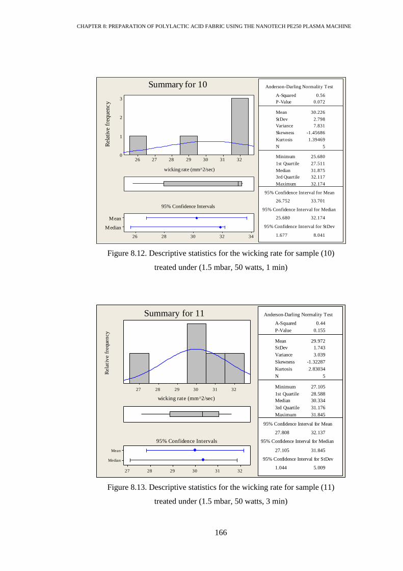
CHAPTER 8: PREPARATION OF POLYLACTIC ACID FABRIC USING THE NANOTECH PE250 PLASMA MACHINE
166
Figure 8.12. Descriptive statistics for the wicking rate for sample (10)
treated under (1.5 mbar, 50 watts, 1 min)
Figure 8.13. Descriptive statistics for the wicking rate for sample (11)
treated under (1.5 mbar, 50 watts, 3 min)
Median
Mean
3432302826
1st Quartile 27.511
Median 31.875
3rd Quartile 32.117
Maximum 32.174
26.752 33.701
25.680 32.174
1.677 8.041
A-Squared 0.56
P-Value 0.072
Mean 30.226
StDev 2.798
Variance 7.831
Skewness -1.45686
Kurtosis 1.39469
N 5
Minimum 25.680
Anderson-Darling Normality Test
95% Confidence Interval for Mean
95% Confidence Interval for Median
95% Confidence Interval for StDev
32313029282726
3
2
1
0
wicking rate (mm^2/sec)
Rel
ativ
e fr
equ
enc
y
95% Confidence Intervals
Summary for 10
323130292827
wicking rate (mm^2/sec)
Rel
ati
ve f
reque
ncy
Median
Mean
323130292827
1st Quartile 28.588
Median 30.334
3rd Quartile 31.176
Maximum 31.845
27.808 32.137
27.105 31.845
1.044 5.009
A-Squared 0.44
P-Value 0.155
Mean 29.972
StDev 1.743
Variance 3.039
Skewness -1.32287
Kurtosis 2.83034
N 5
Minimum 27.105
Anderson-Darling Normality Test
95% Confidence Interval for Mean
95% Confidence Interval for Median
95% Confidence Interval for StDev
95% Confidence Intervals
Summary for 11

CHAPTER 8: PREPARATION OF POLYLACTIC ACID FABRIC USING THE NANOTECH PE250 PLASMA MACHINE
167
Figure 8.14. Descriptive statistics for the wicking rate for sample (12)
treated under (1.5 mbar, 50 watts, 5 min)
8.2.2.2 Box Plot Representation of the Results
A visual comparison of the statistical concepts of the wicking rates of treated and
untreated PLA fabric is illustrated in the Box Plot in Figure 8.15. This chart gives a
graphical representation of the wicking rate distribution around the median and extreme
values.
The plot shows various levels of the deviations of wicking rates after plasma treatment.
Generally speaking these deviations were due to non-stable modification produced by
the plasma treatment. As the surface bombardment by plasma species could result in
topographical and chemical modifications, the level of modifications depends on the
plasma parameters as well as on the substrate, some areas of the substrates were etched
more than others. Some new polar groups appeared on some places on the surface as
suggested in the later sections by XPS and SEM scans, because the plasma can readily
remove the less crystalline area, leading to the formation of a less homogeneous surface.
The experimental condition number (4) exhibited high standard deviation 4.54 mm2/sec
as shown in the descriptive analysis (Figure 8.6), but this result was skewed (Skewness
30282624
wicking rate (mm^2/sec)
Fre
qu
ency
Median
Mean
3230282624
1st Quartile 25.060
Median 25.957
3rd Quartile 29.794
Maximum 31.180
23.811 30.455
24.487 31.180
1.603 7.689
A-Squared 0.30
P-Value 0.412
Mean 27.133
StDev 2.676
Variance 7.160
Skewness 0.974738
Kurtosis -0.029115
N 5
Minimum 24.487
Anderson-Darling Normality Test
95% Confidence Interval for Mean
95% Confidence Interval for Median
95% Confidence Interval for StDev
95% Confidence Intervals
Summary for 12

CHAPTER 8: PREPARATION OF POLYLACTIC ACID FABRIC USING THE NANOTECH PE250 PLASMA MACHINE
168
≈ -1.76), as one replicate (R1) achieved wicking rate very different from the others,
which could be just experimental error.
Figure 8.15. Box plot of wicking rate of untreated (C) and plasma treated fabrics
8.2.2.3 Statistical Comparison of Untreated and Treated Samples
The modifications of wicking behaviour obtained by the plasma treatment were
compared with the control sample in terms of equality of variance and means. Levene’s
test was used to compare the variances of treated samples with the control (untreated).
The results of Levene’s test are presented in Table 8.5. According to Levene’s test most
of the treatment conditions exhibited equal variances with the control, except two cases
(3) and (6) as the probability values (P) were smaller than the significance α = 0.05.
The differences of means between the treated samples and the control according to the t-
test are stated in Table 8.5. The results proved that the mean value of wicking rate
obtained after treatment condition (2) was not statistically different from the control. It
did not achieve improvement in the wicking rate, because the P-value for the t-test was
larger than the pre-selected significance level α = 0.05. All the other test results
demonstrated statistical differences from the mean i.e increased the wicking rate.
121110987654321C
35
30
25
20
15
10
Experiment
wic
kin
g r
ate
(mm
^2/s
ec)
14.82untreated mean

CHAPTER 8: PREPARATION OF POLYLACTIC ACID FABRIC USING THE NANOTECH PE250 PLASMA MACHINE
169
Table 8.5. Levene test and t-test results
Experiment Levene P-value t-test P-value
1 0.098 0.000
2 0.588 0.191
3 0.01 0.004
4 0.360 0.006
5 0.148 0.000
6 0.039 0.000
7 0.348 0.015
8 0.133 0.000
9 0.196 0.000
10 0.671 0.000
11 0.474 0.000
12 0.567 0.000
8.2.2.4 Interaction Plots of Wicking Rate and Processing Parameters
Two independent variables interact if the effect of one of the variables differs,
depending on the level of the other variable. The plots displayed in Figure 8.16
demonstrate the effect of the level of one processing parameter (X axis) on the other
parameter levels in regard to the wicking rate (Y axis).
The plots indicate that a treatment time of (3 min) gave a higher wicking rate when it
was combined with higher power (50 watts) and higher pressure (1.5 mbar). Increasing
the time up to 5 minutes had a detrimental effect on the wicking rate, as can be
concluded from the plots; the wicking rate decreased at 5 minutes whatever the values
of the other variables. Also the graphs illustrated that the pressure and power generally
caused increase in wicking rate when used at their higher levels.

CHAPTER 8: PREPARATION OF POLYLACTIC ACID FABRIC USING THE NANOTECH PE250 PLASMA MACHINE
170
Figure 8.16. Interaction plot of the effect of plasma processing parameters
power, time and pressure on the wicking rate
8.2.2.5 Linear Regression Modelling of the Relationship between Wicking Rate and
Plasma Processing Parameters
A multiple regression model was studied to determine the correlation between the
plasma processing parameters (power, pressure, time) and the productivity (wicking
rate). The regression model obtained is shown in Equation 8.1. This equation could help
in predicting the value of the wicking rate under various plasma processing parameters.
The equation indicated that the wicking rate is function of the intercept (constant) plus
all three plasma processing parameters.
WC = 6.16 + 1.53 Pressure + 0.416 Power + 0.363 Time Equation 8.1
The detailed analysis of the regression model is displayed in Table 8.6. R-sq = 82.4
means that this equation explains 82.4% of the variation in the response (i.e wicking
rate). The results of ANOVA illustrated in Table 8.7 proved that the equation is
statistically significant at the 95% confidence level because P = 0.002 < α = 0.05.
5025 531
30
25
20
30
25
20
Pressure (mbar)
Power (watt)
Time (minutes)
0.5
1.5
pressure
pressure
25
50
power
Interaction Plot for Wc (mm^2/sec)
Data Means

CHAPTER 8: PREPARATION OF POLYLACTIC ACID FABRIC USING THE NANOTECH PE250 PLASMA MACHINE
171
The detailed analysis demonstrated that the pressure, time and the constant value had
each P-value > α = 0.05. This indicated that there were not strong evidences that the
factors had an effect. The pressure and time could be considered effective at a
confidence level greater than 59.8% and 48.7% respectively, while the constant was
effective at a confidence level higher than 87%. The lower confidence found in the
pressure and time could be attributed to the practical application, as the Nanotech
machine is semi-automated, the pressure was adjusted to required level by gauge, and so
the time was watched manually.
Table 8.6. Detailed analysis of the regression model
Predictor Coef SE Coef P
Constant 6.157 3.609 0.126
Pressure 1.533 1.732 0.402
Power 0.41640 0.06926 0.000
Time 0.3631 0.5302 0.513
S = 2.99911 R-Sq = 82.4% R-Sq(adj) = 75.8%
Table 8.7. Analysis of variance
Source DF SS MS F P
Regression 3 336.38 112.13 12.47 0.002
Residual Error 8 71.96 8.99
Total 11 408.33
8.3 Spreading Test
In addition to testing the plasma treated samples for liquid transport in the vertical
direction, the treated samples were also subjected to the micro-drop (volume = 12.50 μl)
spreading test which was explained in Section 4.6. The procedure and modelling of the
drop spreading over the untreated fabric was presented in Section 6.7. The spreading
test was selected because it is a different mechanism of liquid transport from vertical
wicking, as explained in Section 6.7.

CHAPTER 8: PREPARATION OF POLYLACTIC ACID FABRIC USING THE NANOTECH PE250 PLASMA MACHINE
172
In this study, the dynamic of drop spreading after plasma treatment was investigated
using the same steps applied on untreated sample given in Section 6.7. The spreading
rate was assigned to the slope (n) of the (logA, logt) graph which was derived from the
Kissa equation (Equation 6.4).
8.3.1 Experimental Procedure
The design of the experiment was the same as given in Table 8.2. After plasma
treatment, the samples were left in a conditioning room for 24 hours under standard
temperature and relative humidity 22°C (± 2) and 65% (± 2) respectively.
Every treatment condition was repeated and tested five times, and then the average
value was considered.
8.3.2 Experimental Results
Graphs showing the relationship between spreading area (A) and time (t) over PLA
fabrics after plasma preparation are demonstrated in Figure 8.17 given as average value
of five replicas. The logarithmic representation (log A ,log t) of this relationship is
displayed in Figure 8.18. The logarithmic graphs indicated the spreading process
exhibited two phases, in a similar behaviour to that of the untreated sample, but with
different slopes n1 and n2. The average values of the slopes n are given in Table 8.8 and
Table 8.9. The spreading rates of untreated sample were found to be n1= 0.34 and n2=
0.03, as reported in Section 6.7.2.
The first phase (I) was very short, lasting about 1 second, while the second phase (II)
lasted until equilibrium was reached. The following analysis presents a discussion on
the statistical significances of the treated samples and comparison with the untreated
one. The value related to phase I is indicated by (1), and to phase II indicated by (2).

CHAPTER 8: PREPARATION OF POLYLACTIC ACID FABRIC USING THE NANOTECH PE250 PLASMA MACHINE
173
Figure 8.17. Graphical representation of spreading area and time
the number (1-12) refers to the treatment condition as assigned by the design of the
experiment and C is the control sample (untreated).
Figure 8.18 Experimental results of wicking rate (log A, log t) graph
9008007006005004003002001000
250
200
150
100
50
0
Time (second)
Are
a (m
m^
2)
10
11
12
C
1
2
3
4
5
6
7
8
9
3210-1
2.4
2.2
2.0
1.8
1.6
1.4
1.2
logt
logA
0
10
11
12
C
1
2
3
4
5
6
7
8
9
phase I
phase II
Untreated PLA
Untreated PLA

CHAPTER 8: PREPARATION OF POLYLACTIC ACID FABRIC USING THE NANOTECH PE250 PLASMA MACHINE
174
Table 8.8. Values of spreading rate after plasma treatment (phase I)
Experiment Phase I (five repeats) Average n1
1 0.45 0.51 0.47 0.41 0.40 0.45
2 0.39 0.38 0.38 0.37 0.31 0.37
3 0.40 0.50 0.38 0.33 0.32 0.39
4 0.43 0.80 0.79 0.98 0.87 0.77
5 0.15 0.44 0.32 0.29 0.33 0.31
6 0.26 0.44 0.91 0.84 0.55 0.60
7 0.35 0.51 0.22 0.27 0.36 0.34
8 0.32 0.52 0.31 0.42 0.38 0.39
9 0.36 0.27 0.74 0.24 0.43 0.41
10 0.91 0.83 0.97 0.87 0.82 0.88
11 0.35 0.64 0.71 0.88 0.65 0.65
12 0.50 0.42 0.91 0.33 0.47 0.53
n1 for untreated sample = 0.34
Table 8.9. Values of spreading rate after plasma treatment (phase II)
Experiment Phase II (five replicates) Average n2
1 0.05 0.06 0.06 0.06 0.05 0.05
2 0.03 0.03 0.04 0.05 0.05 0.04
3 0.03 0.03 0.03 0.03 0.03 0.03
4 0.12 0.10 0.07 0.11 0.08 0.10
5 0.03 0.06 0.05 0.04 0.05 0.05
6 0.05 0.05 0.06 0.03 0.05 0.05
7 0.05 0.05 0.04 0.05 0.06 0.05
8 0.02 0.03 0.04 0.04 0.04 0.03
9 0.07 0.05 0.09 0.05 0.09 0.07
10 0.07 0.10 0.10 0.08 0.10 0.09
11 0.08 0.12 0.10 0.10 0.11 0.10
12 0.13 0.10 0.11 0.10 0.08 0.11
n2 for untreated sample = 0.03

CHAPTER 8: PREPARATION OF POLYLACTIC ACID FABRIC USING THE NANOTECH PE250 PLASMA MACHINE
175
8.3.3 Statistical Analysis
8.3.3.1 Descriptive Analysis
The graphical summaries of the descriptive analyses of twelve plasma treatment
experiments are presented in the Figures 8.19 to 8.30 (phase I) and Figures 8.31 to 8.42
(phase II). The descriptive analyses provided statistical information on each experiment
including the mean (average), standard deviation, and the spread of data. The
histograms referred to the frequency that each value may occur.
According to the statistical data of phase I, the highest spreading rate achieved was n1 =
0.88 given by treatment recipe number (10). The highest spreading rate noticed in phase
II was n2 = 0.11 given by treatment number (11). However from a statistical prospective
these values cannot be reported as better productivity or achievement. Drawing an
overall idea about the outcome has to take into consideration the mean, standard
deviation, and spread of data, Pareto analysis, and regression modelling. The Anderson-
Darling test for normality distribution proved that all the 24 sets of data were normally
distributed, so they were permissible to be subjected for regression modelling.
Phase I
Figure 8.19. Descriptive statistics of spreading rate for sample (1), phase I
Median
Mean
0.520.500.480.460.440.420.40
1st Quartile 0.40261
Median 0.44979
3rd Quartile 0.49022
Maximum 0.51097
0.38962 0.50456
0.39911 0.51097
0.02773 0.13301
A-Squared 0.23
P-Value 0.624
Mean 0.44709
StDev 0.04629
Variance 0.00214
Skewness 0.38917
Kurtosis -1.18675
N 5
Minimum 0.39911
Anderson-Darling Normality Test
95% Confidence Interval for Mean
95% Confidence Interval for Median
95% Confidence Interval for StDev
0.520.500.480.460.440.420.40
2.0
1.5
1.0
0.5
0.0
Spreading rate (n1)
Fre
qu
enc
y
95% Confidence Intervals
Spreading rate after treatment condition (1)

CHAPTER 8: PREPARATION OF POLYLACTIC ACID FABRIC USING THE NANOTECH PE250 PLASMA MACHINE
176
Figure 8.20. Descriptive statistics of spreading rate for sample (2), phase I
Figure 8.21. Descriptive statistics of spreading rate for sample (3), phase I
Median
Mean
0.420.400.380.360.340.320.30
1st Quartile 0.34164
Median 0.37776
3rd Quartile 0.38744
Maximum 0.39488
0.32813 0.40624
0.31327 0.39488
0.01885 0.09039
A-Squared 0.55
P-Value 0.073
Mean 0.36718
StDev 0.03145
Variance 0.00099
Skewness -1.76875
Kurtosis 3.58762
N 5
Minimum 0.31327
Anderson-Darling Normality Test
95% Confidence Interval for Mean
95% Confidence Interval for Median
95% Confidence Interval for StDev
0.400.380.360.340.32
3
2
1
0
Spreading rate (n2)
Fre
qu
enc
y
95% Confidence Intervals
Spreading rate after treatment condition (2)
0.500.450.400.350.30
Spreading rate (n1)
Fre
qu
en
cy
Median
Mean
0.500.450.400.350.30
1st Quartile 0.32476
Median 0.37626
3rd Quartile 0.45022
Maximum 0.50206
0.29475 0.47573
0.32091 0.50206
0.04366 0.20942
A-Squared 0.34
P-Value 0.327
Mean 0.38524
StDev 0.07288
Variance 0.00531
Skewness 1.23548
Kurtosis 1.46781
N 5
Minimum 0.32091
Anderson-Darling Normality Test
95% Confidence Interval for Mean
95% Confidence Interval for Median
95% Confidence Interval for StDev
95% Confidence Intervals
Spreading rate after treatment condition (3)
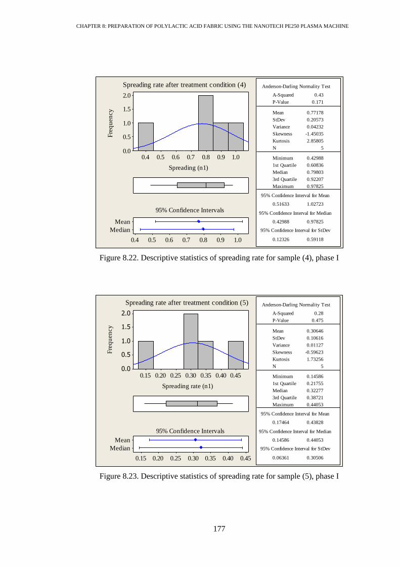
CHAPTER 8: PREPARATION OF POLYLACTIC ACID FABRIC USING THE NANOTECH PE250 PLASMA MACHINE
177
Figure 8.22. Descriptive statistics of spreading rate for sample (4), phase I
Figure 8.23. Descriptive statistics of spreading rate for sample (5), phase I
Median
Mean
1.00.90.80.70.60.50.4
1st Quartile 0.60836
Median 0.79803
3rd Quartile 0.92207
Maximum 0.97825
0.51633 1.02723
0.42988 0.97825
0.12326 0.59118
A-Squared 0.43
P-Value 0.171
Mean 0.77178
StDev 0.20573
Variance 0.04232
Skewness -1.45035
Kurtosis 2.85805
N 5
Minimum 0.42988
Anderson-Darling Normality Test
95% Confidence Interval for Mean
95% Confidence Interval for Median
95% Confidence Interval for StDev
1.00.90.80.70.60.50.4
2.0
1.5
1.0
0.5
0.0
Spreading (n1)
Fre
qu
en
cy
95% Confidence Intervals
Spreading rate after treatment condition (4)
0.450.400.350.300.250.200.15
2.0
1.5
1.0
0.5
0.0
Spreading rate (n1)
Fre
qu
en
cy
Median
Mean
0.450.400.350.300.250.200.15
1st Quartile 0.21755
Median 0.32277
3rd Quartile 0.38721
Maximum 0.44053
0.17464 0.43828
0.14586 0.44053
0.06361 0.30506
A-Squared 0.28
P-Value 0.475
Mean 0.30646
StDev 0.10616
Variance 0.01127
Skewness -0.59623
Kurtosis 1.73256
N 5
Minimum 0.14586
Anderson-Darling Normality Test
95% Confidence Interval for Mean
95% Confidence Interval for Median
95% Confidence Interval for StDev
95% Confidence Intervals
Spreading rate after treatment condition (5)

CHAPTER 8: PREPARATION OF POLYLACTIC ACID FABRIC USING THE NANOTECH PE250 PLASMA MACHINE
178
Figure 8.24. Descriptive statistics of spreading rate for sample (6), phase I
Figure 8.25. Descriptive statistics of spreading rate for sample (7), phase I
Median
Mean
1.00.80.60.40.2
1st Quartile 0.35161
Median 0.54514
3rd Quartile 0.87533
Maximum 0.91322
0.26148 0.93813
0.26192 0.91322
0.16325 0.78298
A-Squared 0.23
P-Value 0.621
Mean 0.59980
StDev 0.27248
Variance 0.07424
Skewness 0.03061
Kurtosis -1.98797
N 5
Minimum 0.26192
Anderson-Darling Normality Test
95% Confidence Interval for Mean
95% Confidence Interval for Median
95% Confidence Interval for StDev
0.90.80.70.60.50.40.3
1.00
0.75
0.50
0.25
0.00
Spreading rate (n1)
Fre
qu
en
cy
95% Confidence Intervals
Spreading rate after treatment condition (6)
0.500.450.400.350.300.250.20
2.0
1.5
1.0
0.5
0.0
Spreading rate (n1)
Fre
qu
en
cy
Median
Mean
0.500.450.400.350.300.250.20
1st Quartile 0.24421
Median 0.34932
3rd Quartile 0.43723
Maximum 0.51447
0.20234 0.48253
0.21528 0.51447
0.06760 0.32422
A-Squared 0.25
P-Value 0.571
Mean 0.34244
StDev 0.11283
Variance 0.01273
Skewness 0.785465
Kurtosis 0.949894
N 5
Minimum 0.21528
Anderson-Darling Normality Test
95% Confidence Interval for Mean
95% Confidence Interval for Median
95% Confidence Interval for StDev
95% Confidence Intervals
Spreading rate after treatment condition (7)

CHAPTER 8: PREPARATION OF POLYLACTIC ACID FABRIC USING THE NANOTECH PE250 PLASMA MACHINE
179
Figure 8.26. Descriptive statistics of spreading rate for sample (8), phase I
Figure 8.27. Descriptive statistics of spreading rate for sample (9), phase I
0.500.450.400.350.30
2.0
1.5
1.0
0.5
0.0
Spreading rate (n1)
Fre
qu
enc
y
Median
Mean
0.550.500.450.400.350.30
1st Quartile 0.31156
Median 0.38196
3rd Quartile 0.47242
Maximum 0.52238
0.28068 0.49929
0.30669 0.52238
0.05274 0.25296
A-Squared 0.26
P-Value 0.525
Mean 0.38998
StDev 0.08803
Variance 0.00775
Skewness 0.842191
Kurtosis 0.031022
N 5
Minimum 0.30669
Anderson-Darling Normality Test
95% Confidence Interval for Mean
95% Confidence Interval for Median
95% Confidence Interval for StDev
95% Confidence Intervals
Spreading rate after treatment condition (8)
0.70.60.50.40.30.2
Spreading rate (n1)
Fre
qu
en
cy
Median
Mean
0.80.70.60.50.40.30.2
1st Quartile 0.25638
Median 0.36162
3rd Quartile 0.58258
Maximum 0.73762
0.16140 0.65443
0.24047 0.73762
0.11895 0.57051
A-Squared 0.40
P-Value 0.207
Mean 0.40791
StDev 0.19854
Variance 0.03942
Skewness 1.52079
Kurtosis 2.41645
N 5
Minimum 0.24047
Anderson-Darling Normality Test
95% Confidence Interval for Mean
95% Confidence Interval for Median
95% Confidence Interval for StDev
95% Confidence Intervals
Spreading rate after treatment condition (9)

CHAPTER 8: PREPARATION OF POLYLACTIC ACID FABRIC USING THE NANOTECH PE250 PLASMA MACHINE
180
Figure 8.28. Descriptive statistics of spreading rate for sample (10), phase I
Figure 8.29. Descriptive statistics of spreading rate for sample (11), phase I
0.9750.9500.9250.9000.8750.8500.825
2.0
1.5
1.0
0.5
0.0
Spreading rate (n1)
Fre
qu
en
cy
Median
Mean
0.960.920.880.840.80
1st Quartile 0.82364
Median 0.87079
3rd Quartile 0.93836
Maximum 0.97052
0.80198 0.95594
0.81807 0.97052
0.03715 0.17816
A-Squared 0.23
P-Value 0.611
Mean 0.87896
StDev 0.06200
Variance 0.00384
Skewness 0.766459
Kurtosis -0.325812
N 5
Minimum 0.81807
Anderson-Darling Normality Test
95% Confidence Interval for Mean
95% Confidence Interval for Median
95% Confidence Interval for StDev
95% Confidence Intervals
Spreading rate after treatment condition (10)
0.90.80.70.60.50.4
2.0
1.5
1.0
0.5
0.0
Spreading rate (n1)
Fre
qu
en
cy
Median
Mean
0.90.80.70.60.50.40.3
1st Quartile 0.49639
Median 0.65164
3rd Quartile 0.79566
Maximum 0.87778
0.41135 0.88295
0.35290 0.87778
0.11378 0.54571
A-Squared 0.31
P-Value 0.384
Mean 0.64715
StDev 0.18991
Variance 0.03606
Skewness -0.78590
Kurtosis 1.94299
N 5
Minimum 0.35290
Anderson-Darling Normality Test
95% Confidence Interval for Mean
95% Confidence Interval for Median
95% Confidence Interval for StDev
95% Confidence Intervals
Spreading rate after treatment condition (11)

CHAPTER 8: PREPARATION OF POLYLACTIC ACID FABRIC USING THE NANOTECH PE250 PLASMA MACHINE
181
Figure 8.30. Descriptive statistics of spreading rate for sample (12), phase I
Phase 2
Figure 8.31. Descriptive statistics of spreading rate for sample (1), phase II
Median
Mean
1.00.80.60.40.2
1st Quartile 0.37710
Median 0.46968
3rd Quartile 0.70348
Maximum 0.91010
0.24824 0.80409
0.32963 0.91010
0.13411 0.64320
A-Squared 0.55
P-Value 0.074
Mean 0.52617
StDev 0.22383
Variance 0.05010
Skewness 1.77408
Kurtosis 3.62181
N 5
Minimum 0.32963
Anderson-Darling Normality Test
95% Confidence Interval for Mean
95% Confidence Interval for Median
95% Confidence Interval for StDev
0.90.80.70.60.50.40.3
2.0
1.5
1.0
0.5
0.0
Spreading rate (n1)
Fre
qu
en
cy
95% Confidence Intervals
Spreading rate after treatment condition (12)
Median
Mean
0.0650.0600.0550.0500.045
1st Quartile 0.046740
Median 0.055367
3rd Quartile 0.061827
Maximum 0.063708
0.044851 0.064150
0.045016 0.063708
0.004656 0.022332
A-Squared 0.20
P-Value 0.767
Mean 0.054500
StDev 0.007771
Variance 0.000060
Skewness -0.11562
Kurtosis -2.00670
N 5
Minimum 0.045016
Anderson-Darling Normality Test
95% Confidence Interval for Mean
95% Confidence Interval for Median
95% Confidence Interval for StDev
0.0650.0600.0550.0500.045
1.2
0.9
0.6
0.3
0.0
Spreading rate (n2)
Fre
qu
en
cy
95% Confidence Intervals
Spreading rate after treatment condition (1)

CHAPTER 8: PREPARATION OF POLYLACTIC ACID FABRIC USING THE NANOTECH PE250 PLASMA MACHINE
182
Figure 8.32. Descriptive statistics of spreading rate for sample (2), phase II
Figure 8.33. Descriptive statistics of spreading rate for sample (3), phase II
Median
Mean
0.0550.0500.0450.0400.0350.030
1st Quartile 0.032241
Median 0.038420
3rd Quartile 0.049213
Maximum 0.052112
0.029261 0.051271
0.030643 0.052112
0.005310 0.025468
A-Squared 0.21
P-Value 0.713
Mean 0.040266
StDev 0.008863
Variance 0.000079
Skewness 0.43159
Kurtosis -1.65432
N 5
Minimum 0.030643
Anderson-Darling Normality Test
95% Confidence Interval for Mean
95% Confidence Interval for Median
95% Confidence Interval for StDev
0.0500.0450.0400.0350.030
1.00
0.75
0.50
0.25
0.00
Spreading rate (n2)
Fre
qu
en
cy
95% Confidence Intervals
Spreading rate after treatment condition (2)
0.0350.0340.0330.0320.0310.0300.029
1.00
0.75
0.50
0.25
0.00
Spreading rate (n2)
Fre
qu
en
cy
Median
Mean
0.03600.03450.03300.03150.0300
1st Quartile 0.029759
Median 0.032395
3rd Quartile 0.034374
Maximum 0.034949
0.029152 0.035112
0.029053 0.034949
0.001438 0.006897
A-Squared 0.17
P-Value 0.845
Mean 0.032132
StDev 0.002400
Variance 0.000006
Skewness -0.20554
Kurtosis -1.66045
N 5
Minimum 0.029053
Anderson-Darling Normality Test
95% Confidence Interval for Mean
95% Confidence Interval for Median
95% Confidence Interval for StDev
95% Confidence Intervals
Spreading rate after treatment condition (3)

CHAPTER 8: PREPARATION OF POLYLACTIC ACID FABRIC USING THE NANOTECH PE250 PLASMA MACHINE
183
Figure 8.34. Descriptive statistics of spreading rate for sample (4), phase II
Figure 8.35. Descriptive statistics of spreading rate for sample (5), phase II
0.120.110.100.090.080.07
1.00
0.75
0.50
0.25
0.00
Spreading rate (n2)
Fre
qu
en
cy
Median
Mean
0.120.110.100.090.080.07
1st Quartile 0.076171
Median 0.102859
3rd Quartile 0.111122
Maximum 0.115671
0.072465 0.118514
0.071452 0.115671
0.011110 0.053285
A-Squared 0.29
P-Value 0.462
Mean 0.095489
StDev 0.018543
Variance 0.000344
Skewness -0.45855
Kurtosis -2.04559
N 5
Minimum 0.071452
Anderson-Darling Normality Test
95% Confidence Interval for Mean
95% Confidence Interval for Median
95% Confidence Interval for StDev
95% Confidence Intervals
Spreading rate after treatment condition (4)
0.0550.0500.0450.0400.0350.030
2.0
1.5
1.0
0.5
0.0
Spreading rate (n2)
Fre
qu
en
cy
Median
Mean
0.0600.0550.0500.0450.0400.0350.030
1st Quartile 0.036016
Median 0.051637
3rd Quartile 0.055830
Maximum 0.056737
0.033743 0.060388
0.031538 0.056737
0.006428 0.030831
A-Squared 0.34
P-Value 0.328
Mean 0.047066
StDev 0.010729
Variance 0.000115
Skewness -0.85769
Kurtosis -1.11468
N 5
Minimum 0.031538
Anderson-Darling Normality Test
95% Confidence Interval for Mean
95% Confidence Interval for Median
95% Confidence Interval for StDev
95% Confidence Intervals
Spreading rate after treatment condition (5)

CHAPTER 8: PREPARATION OF POLYLACTIC ACID FABRIC USING THE NANOTECH PE250 PLASMA MACHINE
184
Figure 8.36. Descriptive statistics of spreading rate for sample (6), phase II
Figure 8.37. Descriptive statistics of spreading rate for sample (7), phase II
Median
Mean
0.0600.0550.0500.0450.0400.035
1st Quartile 0.039473
Median 0.046844
3rd Quartile 0.052500
Maximum 0.057537
0.035722 0.056593
0.033927 0.057537
0.005035 0.024151
A-Squared 0.32
P-Value 0.378
Mean 0.046158
StDev 0.008405
Variance 0.000071
Skewness -0.24934
Kurtosis 1.80782
N 5
Minimum 0.033927
Anderson-Darling Normality Test
95% Confidence Interval for Mean
95% Confidence Interval for Median
95% Confidence Interval for StDev
0.0600.0550.0500.0450.0400.035
3
2
1
0
Spreading rate (n2)
Fre
qu
en
cy
95% Confidence Intervals
Spreading rate after treatment condition (6)
Median
Mean
0.05750.05500.05250.05000.04750.0450
1st Quartile 0.046177
Median 0.053950
3rd Quartile 0.054963
Maximum 0.055966
0.044917 0.057575
0.043387 0.055966
0.003054 0.014647
A-Squared 0.38
P-Value 0.244
Mean 0.051246
StDev 0.005097
Variance 0.000026
Skewness -1.10869
Kurtosis 0.23432
N 5
Minimum 0.043387
Anderson-Darling Normality Test
95% Confidence Interval for Mean
95% Confidence Interval for Median
95% Confidence Interval for StDev
0.0560.0540.0520.0500.0480.0460.044
2.0
1.5
1.0
0.5
0.0
Spreading rate (n2)
Fre
qu
en
cy
95% Confidence Intervals
Spreading rate after treatment condition (7)

CHAPTER 8: PREPARATION OF POLYLACTIC ACID FABRIC USING THE NANOTECH PE250 PLASMA MACHINE
185
Figure 8.38. Descriptive statistics of spreading rate for sample (8), phase II
Figure 8.39. Descriptive statistics of spreading rate for sample (9), phase II
Median
Mean
0.0400.0350.0300.0250.020
1st Quartile 0.023578
Median 0.035840
3rd Quartile 0.037893
Maximum 0.039786
0.022129 0.041383
0.021636 0.039786
0.004645 0.022280
A-Squared 0.37
P-Value 0.259
Mean 0.031756
StDev 0.007753
Variance 0.000060
Skewness -0.55132
Kurtosis -2.20263
N 5
Minimum 0.021636
Anderson-Darling Normality Test
95% Confidence Interval for Mean
95% Confidence Interval for Median
95% Confidence Interval for StDev
0.0400.0350.0300.0250.020
2.0
1.5
1.0
0.5
0.0
Spreading rate (n2)
Fre
qu
en
cy
95% Confidence Intervals
Spreading rate after treatment condition (8)
0.090.080.070.060.05
2.0
1.5
1.0
0.5
0.0
Spreading rate (n2)
Fre
qu
en
cy
Median
Mean
0.100.090.080.070.060.050.04
1st Quartile 0.051317
Median 0.067765
3rd Quartile 0.089776
Maximum 0.090887
0.045967 0.094014
0.049131 0.090887
0.011592 0.055597
A-Squared 0.34
P-Value 0.332
Mean 0.069990
StDev 0.019348
Variance 0.000374
Skewness 0.11905
Kurtosis -2.86567
N 5
Minimum 0.049131
Anderson-Darling Normality Test
95% Confidence Interval for Mean
95% Confidence Interval for Median
95% Confidence Interval for StDev
95% Confidence Intervals
Spreading rate after treatment condition (9)

CHAPTER 8: PREPARATION OF POLYLACTIC ACID FABRIC USING THE NANOTECH PE250 PLASMA MACHINE
186
Figure 8.40. Descriptive statistics of spreading rate for sample (10), phase II
Figure 8.41. Descriptive statistics of spreading rate for sample (11), phase II
Median
Mean
0.110.100.090.080.07
1st Quartile 0.074688
Median 0.098150
3rd Quartile 0.101170
Maximum 0.103024
0.071894 0.108052
0.069385 0.103024
0.008723 0.041839
A-Squared 0.41
P-Value 0.194
Mean 0.089973
StDev 0.014560
Variance 0.000212
Skewness -0.82829
Kurtosis -1.58373
N 5
Minimum 0.069385
Anderson-Darling Normality Test
95% Confidence Interval for Mean
95% Confidence Interval for Median
95% Confidence Interval for StDev
0.100.090.080.07
2.0
1.5
1.0
0.5
0.0
Spreading rate (n2)
Fre
qu
enc
y
95% Confidence Intervals
Spreading rate after treatment condition (10)
0.120.110.100.090.08
2.0
1.5
1.0
0.5
0.0
Spreading rate (n2)
Fre
qu
en
cy
Median
Mean
0.120.110.100.090.08
1st Quartile 0.09176
Median 0.10373
3rd Quartile 0.11602
Maximum 0.12299
0.08543 0.12228
0.08188 0.12299
0.00889 0.04264
A-Squared 0.24
P-Value 0.575
Mean 0.10385
StDev 0.01484
Variance 0.00022
Skewness -0.44329
Kurtosis 1.48426
N 5
Minimum 0.08188
Anderson-Darling Normality Test
95% Confidence Interval for Mean
95% Confidence Interval for Median
95% Confidence Interval for StDev
95% Confidence Intervals
Spreading rate after treatment condition (11)

CHAPTER 8: PREPARATION OF POLYLACTIC ACID FABRIC USING THE NANOTECH PE250 PLASMA MACHINE
187
Figure 8.42. Descriptive statistics of spreading rate for sample (12), phase II
8.3.3.2 Statistical Comparison of Treated and Untreated Samples
The results of spreading rates achieved after plasma treatment were compared with the
control sample in terms of equality of variance and means. As previously reported in
Section (8.2.3.3) the Levene test can be used for comparing the variances, and the t-test
for comparing the means. The results of Levene and t-test are shown in
and Table 8.11 for phases I and II respectively.
In phase I, experiment (6) exhibited different variances from the control sample because
P-value = 0.01 < α = 0.05, so the t-test for this experiment was done on the assumption
of unequal variance. The results of the t-test proved that treatment conditions (1) (4)
(10) (11) gave statistically different means from the untreated one in phase I. The other
treatment conditions showed no statistical differences from the mean on average level,
though there were some experiments exhibited higher spreading rates, this could be
attributed to place at the fabric where the droplet fell down, which indicated that the
surface was not homogeneously modified.
With regard to phase II, the Levene test indicated that the treatment conditions (4) and
(9) resulted in unequal variances to the control sample. The t-test demonstrated the
treatment conditions (1 ,4 ,5 ,6 ,7 ,9 ,10 ,11 ,12) achieved statistically different means,
0.130.120.110.100.090.08
2.0
1.5
1.0
0.5
0.0
Spreading rate (n2)
Fre
qu
en
cy
Median
Mean
0.140.130.120.110.100.090.08
1st Quartile 0.08958
Median 0.10316
3rd Quartile 0.12339
Maximum 0.13393
0.08061 0.13102
0.07787 0.13393
0.01216 0.05833
A-Squared 0.22
P-Value 0.670
Mean 0.10582
StDev 0.02030
Variance 0.00041
Skewness 0.03160
Kurtosis 1.10988
N 5
Minimum 0.07787
Anderson-Darling Normality Test
95% Confidence Interval for Mean
95% Confidence Interval for Median
95% Confidence Interval for StDev
95% Confidence Intervals
Spreading rate after treatment condition (12)

CHAPTER 8: PREPARATION OF POLYLACTIC ACID FABRIC USING THE NANOTECH PE250 PLASMA MACHINE
188
while for the conditions (2, 3, 8) the means of the treated samples were not statistically
different from that of the untreated fabric.
There were differences in reaction to plasma between phases I and II, which could be
related to differences in the mechanism of spreading explained in Section (4.6).
Table 8.10. Results of Levene and t-test for phase I
Table 8.11. Results of Levene and t-test for phase II
Experiment number Levene test P-value t- test P-value
1 0.206 0.004
2 0.050 0.275
3 0.648 0.253
4 0.218 0.010
5 0.817 0.603
6 0.010 0.100
7 0.578 0.907
8 0.888 0.275
9 0.166 0.475
10 0.487 0.000
11 0.211 0.024
12 0.250 0.138
Experiment number Levene test P-value t-test P-value
1 0.145 0.001
2 0.104 0.056
3 0.200 0.220
4 0.023 0.001
5 0.118 0.026
6 0.437 0.010
7 0.978 0.000
8 0.33 0.633
9 0.002 0.010
10 0.095 0.001
11 0.080 0.000
12 0.038 0.001

CHAPTER 8: PREPARATION OF POLYLACTIC ACID FABRIC USING THE NANOTECH PE250 PLASMA MACHINE
189
8.3.3.3 Box Plot Representation of the Results
Graphical illustrations of the comparisons between the spreading rates of treated and
untreated samples during phases I and II are given by the box plots in Figure 8.43 and
Figure 8.44 respectively. The Figures visually exhibit the dispersion of treated-sample
data around the untreated one. It was concluded that the treatment condition number (6)
resulted in the highest variation in the spreading during phase I, while the highest
variation in phase II was attributed to treatment condition number (9). The box plot and
the results of the Levene’s and t-test, given in Table 8.11 clarified differences between
phases I and II in the reaction of the substrate to plasma treatment condition. For
example, the conditions (5) (6) (7) (9) (12) produced means statistically equal to the
untreated sample in phase I because the probability value P > α = 0.05. In contrast, these
conditions produced different means from the untreated sample in phase II as the
probability values were P < α = 0.05.
Other noticeable results were that the conditions (2) and (3) produced means equal to
the untreated sample mean in phases I and II.
Another difference detected in the level of variation between phases I and II was that
experiment (6) produced an improvement in spreading rate (n1) but with very high
variation in phase I, while the variation was smaller in phase II as can be seen on the
box plot. This could be attributed to the various levels of physical and chemical effects
of each plasma processing combination (pressure, power, time), and the complicated
nature of micro drop spreading which involves differences in mechanisms of spreading
between phases I and II as reported in Section (4.6).
In conclusion there was no correlation in responses to plasma treatment between phases
I and II. This could be related to the different mechanism involved in the spreading
between phases I and II as explained in Section 4.6. In addition, phase I was measured
during the short time of 1 second on an irregular textile surface, therefore it may involve
relatively high error and it did not exhibit clear trend in response to plasma parameters.

CHAPTER 8: PREPARATION OF POLYLACTIC ACID FABRIC USING THE NANOTECH PE250 PLASMA MACHINE
190
Figure 8.43. Spreading rates of samples treated by plasma in phase I.
C is the untreated sample
Figure 8.44. Spreading rates of samples treated by plasma in phase II.
C is the untreated sample
121110987654321C
1.0
0.9
0.8
0.7
0.6
0.5
0.4
0.3
0.2
0.1
Experiment
Sp
read
ing r
ate
(n1
)
0.3356
121110987654321C
0.14
0.12
0.10
0.08
0.06
0.04
0.02
Experiment
Sp
read
ing
rate
(n2
)
0.0299
Untreated mean
Untreated mean

CHAPTER 8: PREPARATION OF POLYLACTIC ACID FABRIC USING THE NANOTECH PE250 PLASMA MACHINE
191
8.3.3.4 Regression Model of Spreading Rate (n) versus Plasma Parameters
Pressure, Power, and Time
The regression model of spreading behaviour was investigated to try to correlate the
modifications in the spreading rates with the plasma processing parameters, so they
could be used in future work to predict the spreading rate under various plasma
treatment recipes.
The spreading process was found to be split into two phases controlled by different
mechanisms as explained in section 4.6. Therefore the spreading process during phase I
and II is expected to react differently to the physical and chemical modifications
produced by plasma treatment as presented in later sections (8.5) and (8.6), hence the
relationships between plasma parameters and spreading rates were studied by two
different models for phases I and II.
The regression models were established depending on the values of n1 and n2 presented
in Table 8.8 and Table 8.9, and the experimental design of the plasma parameters given
in Table 8.3.
Phase I
Regression analysis was run of n1 versus pressure, power, and time. The regression
model found was
n1 = 0.205 + 0.052 pressure + 0.00925 power - 0.0328 time Equation 8.2
where the units of pressure, power and time are mbar, watts, and minutes respectively
The detailed analysis and the analysis of variance of the regression model is shown in
Table 8.12 and Table 8.13 respectively. R-sq = 55.5% expresses the percentage of the
variation in the dependant variable that is explained by variation in the independent
variable. The probability value of the analysis of variance P = 0.077 indicated the model
could not perform at the pre-determined confidence level of this research 95%, however
it is still accepted at 92% confidence level, therefore it can be concluded at 92%
confidence the null hypothesis (the independent variable does not affect the dependant)
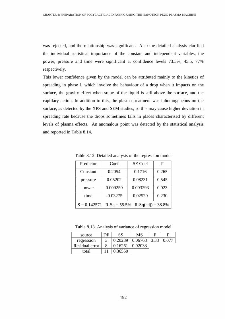
CHAPTER 8: PREPARATION OF POLYLACTIC ACID FABRIC USING THE NANOTECH PE250 PLASMA MACHINE
192
was rejected, and the relationship was significant. Also the detailed analysis clarified
the individual statistical importance of the constant and independent variables; the
power, pressure and time were significant at confidence levels 73.5%, 45.5, 77%
respectively.
This lower confidence given by the model can be attributed mainly to the kinetics of
spreading in phase I, which involve the behaviour of a drop when it impacts on the
surface, the gravity effect when some of the liquid is still above the surface, and the
capillary action. In addition to this, the plasma treatment was inhomogeneous on the
surface, as detected by the XPS and SEM studies, so this may cause higher deviation in
spreading rate because the drops sometimes falls in places characterised by different
levels of plasma effects. An anomalous point was detected by the statistical analysis
and reported in Table 8.14.
Table 8.12. Detailed analysis of the regression model
Predictor Coef SE Coef P
Constant 0.2054 0.1716 0.265
pressure 0.05202 0.08231 0.545
power 0.009250 0.003293 0.023
time -0.03275 0.02520 0.230
S = 0.142571 R-Sq = 55.5% R-Sq(adj) = 38.8%
Table 8.13. Analysis of variance of regression model
source DF SS MS F P
regression 3 0.20289 0.06763 3.33 0.077
Residual error 8 0.16261 0.02033
total 11 0.36550

CHAPTER 8: PREPARATION OF POLYLACTIC ACID FABRIC USING THE NANOTECH PE250 PLASMA MACHINE
193
Table 8.14. Unusual observation, R denotes an observation with a large standardised
residual
Unusual observation (anomalous point)
Observation pressure n1 Fit Se Fit Residual St Resit
Experiment 5 0.50 0.3100 0.5842 0.0732 -0.2742 -2.16R
Phase 2
The regression analysis of n2 versus pressure, power, and time, resulted in the following
model
n2 = - 0.0054 + 0.0215 pressure + 0.00144 power - 0.00184 time Equation 8.3
where the units of pressure, power and time are mbar, watts, and minutes respectively
The detailed analysis and the analysis of variance of the regression model are presented
in Table 8.15 and Table 8.16. The analysis of variance indicated that the model was
significant at confidence level 95%, because the probability value P = 0.031 < α = 0.05
(the pre-selected confidence level given in Chapter 5). The detailed analysis stated that
the power was significant at confidence level 95%, while the constant, pressure and
time were significant at 18.1%, 91.4 and 40%. This lower significance level could be
attributed to the same reasons as those presented in the previous paragraph.
Table 8.15. Detailed analysis of the regression model
predictor Coef SE Coef P
constant -0.00543 0.02290 0.819
pressure 0.02155 0.01099 0.086
power 0.0014413 0.0004396 0.011
time -0.001836 0.003365 0.600
S = 0.0190331 R-Sq = 65.1% R-Sq(adj) = 52.0%
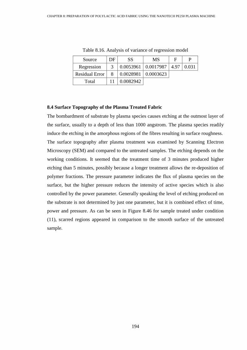
CHAPTER 8: PREPARATION OF POLYLACTIC ACID FABRIC USING THE NANOTECH PE250 PLASMA MACHINE
194
Table 8.16. Analysis of variance of regression model
Source DF SS MS F P
Regression 3 0.0053961 0.0017987 4.97 0.031
Residual Error 8 0.0028981 0.0003623
Total 11 0.0082942
8.4 Surface Topography of the Plasma Treated Fabric
The bombardment of substrate by plasma species causes etching at the outmost layer of
the surface, usually to a depth of less than 1000 angstrom. The plasma species readily
induce the etching in the amorphous regions of the fibres resulting in surface roughness.
The surface topography after plasma treatment was examined by Scanning Electron
Microscopy (SEM) and compared to the untreated samples. The etching depends on the
working conditions. It seemed that the treatment time of 3 minutes produced higher
etching than 5 minutes, possibly because a longer treatment allows the re-deposition of
polymer fractions. The pressure parameter indicates the flux of plasma species on the
surface, but the higher pressure reduces the intensity of active species which is also
controlled by the power parameter. Generally speaking the level of etching produced on
the substrate is not determined by just one parameter, but it is combined effect of time,
power and pressure. As can be seen in Figure 8.46 for sample treated under condition
(11), scarred regions appeared in comparison to the smooth surface of the untreated
sample.
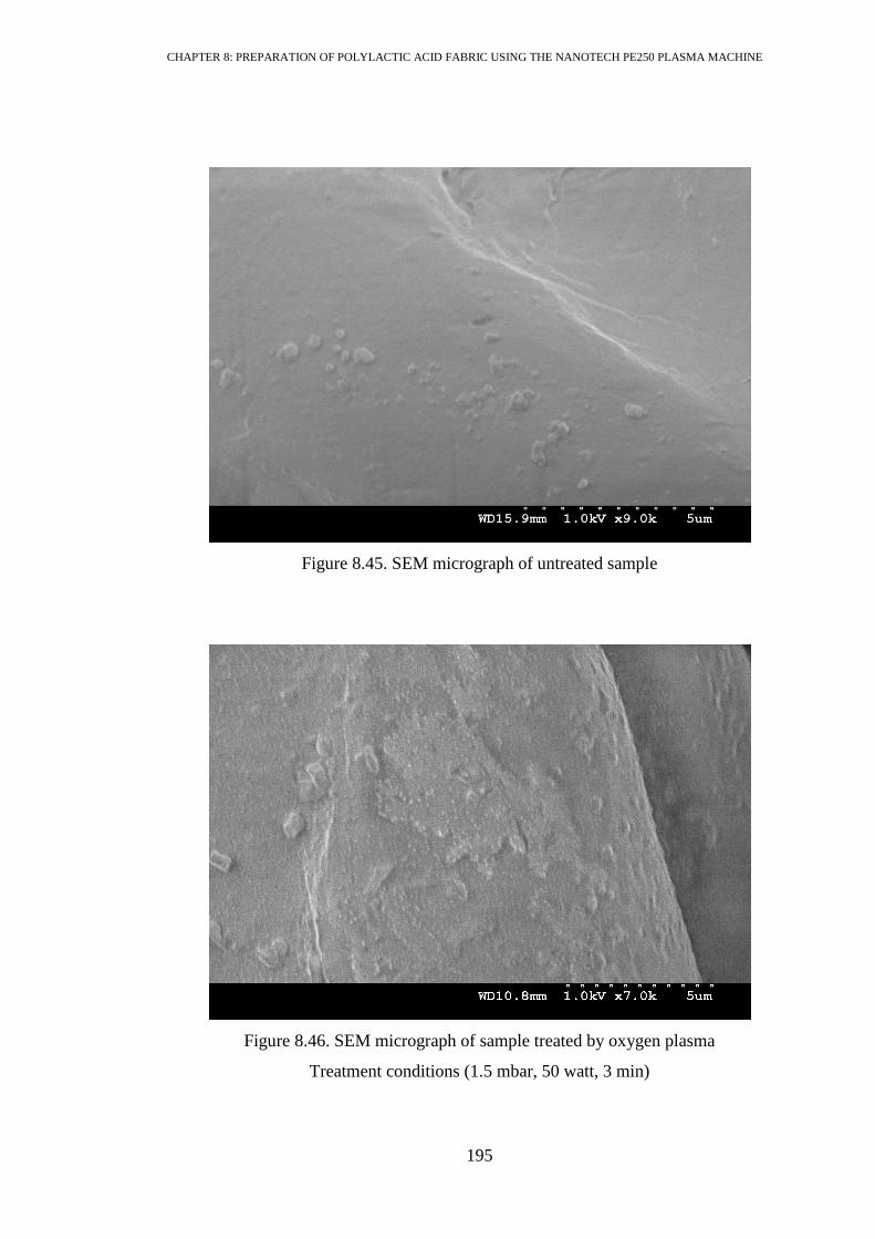
CHAPTER 8: PREPARATION OF POLYLACTIC ACID FABRIC USING THE NANOTECH PE250 PLASMA MACHINE
195
Figure 8.45. SEM micrograph of untreated sample
Figure 8.46. SEM micrograph of sample treated by oxygen plasma
Treatment conditions (1.5 mbar, 50 watt, 3 min)

CHAPTER 8: PREPARATION OF POLYLACTIC ACID FABRIC USING THE NANOTECH PE250 PLASMA MACHINE
196
8.5 Chemical Composition of Plasma Treated PLA Fabric
The etching revealed in the previous section by the SEM scan, could result in chain
scission of PLA molecules on the surface, causing a decrease in the carbon content on
the surface and possible reaction with O2 leading to the formation of new functional
groups.
The general possible interaction positions in PLA molecule are the relatively weaker
chemical bonds in the chain. The chemical bonds in PLA are C=O, C-C, C-O, C-H. The
bond energies of these groups are given in Table 8.17. The C=O bond has the greatest
bonding energy, therefore C-C, C-O, and the C-H bonds have higher probability of
chain scission than C=O bond.
Table 8.17. Bond energy of common chemical bonds in polymer [201]
Chemical bond Bond energy (eV)
C-H 4.3
C-C 3.6
C-O 3.7
C=C 6.3
In order to reveal what modifications were initiated on the PLA surface, the samples
were examined by X-ray photoelectron spectroscopy (XPS). The XPS results of the
treated samples were compared with that of untreated PLA which was presented in
Chapter 6.
The samples that were statistically proved to have achieved modifications in wicking
and spreading rates were subjected to XPS examination. Taking into consideration the
results of the t-test for wicking and spreading rates given in Table 8.5, and Table 8.11, it
was concluded that statistically different means from the untreated sample were
obtained under treatment conditions (1), (4), (10), (11). In addition to this, sample
number (5) was examined by XPS because it gave the highest wicking rate.
The Figures 47-56 illustrate the survey scans and C1s spectra of the five plasma treated
samples (1), (4), (5), (10), and (11), as well the relative chemical compositions. The
proportions of the chemical groups are given in Table 8.18 and Table 8.19.

CHAPTER 8: PREPARATION OF POLYLACTIC ACID FABRIC USING THE NANOTECH PE250 PLASMA MACHINE
197
Sample (1) appeared similar to the untreated one, with no new chemical groups detected
on the surface. The slight change in wicking and spreading rate in this case, could be
attributed to physical modifications of the surface due to ion bombardment, such as
changing the fibre arrangement or etching, as highlighted in the SEM images (see
Section 8.5).
The deconvolution analysis C1s of the samples (4), (5), (10) and (11) showed new COO
groups at 299.7 eV. The atomic ratios of these samples exhibited an increase in O/C
percentage after plasma treatment.
It can be assumed that during exposure to oxygen plasma treatment in the Nanotech
machine, polymer surfaces interact with oxygen ions and electrons which are the
activated species in the oxygen plasma, causing scission of C-H and C-C bonds. As a
result of the C-H bond scission, hydrogen atoms are eliminated from the polymer chain
and carbon radicals are formed in the middle of the polymer chain. On the other hand,
in the C-C bond scission process, two carbon radicals are formed at the end position of
the polymer chain. These carbon radicals at the middle and end positions of the polymer
chains are successively oxidised into carboxyl functional groups when the substrate is
taken out from the plasma reactor after finishing the plasma processing.
Therefore it seemed that the plasma treatment caused the incorporation of oxygen
moieties into the PLA surface, which resulted in an increase in the wicking rate and
spreading.
Table 8.18. Relative element ratios
Relative element ratios
Data Set C 1s % N 1s % O 1s % O/C%
C (untreated) 64.70 0.21 35.09 54.23
1 65.44 0.23 34.33 52.47
4 61.21 0.05 38.74 63.28
5 60.35 0.36 39.29 65.1
10 58.66 0.15 41.19 70.21
11 62.11 0.20 37.69 60.69

CHAPTER 8: PREPARATION OF POLYLACTIC ACID FABRIC USING THE NANOTECH PE250 PLASMA MACHINE
198
Table 8.19. Deconvolution of C1s Spectra for PLA samples treated by
oxygen plasma
Relative ratios of C 1s peaks
Data Set C-C or C-H C-O C=O COO
C (untreated) 42.56 24.24 33.20 0.00
1 38.94 26.50 34.55 0.01
4 28.39 29.24 36.83 5.54
5 24.97 26.67 32.61 15.75
10 20.13 26.57 39.99 13.31
11 16.64 29.75 35.52 18.09
Figure 8.47. Survey scan of sample (1)
0
10000
20000
30000
40000
50000
60000
70000
80000
90000
0 500 1000 1500
count
per
sec
ond
Be (eV)
survey scan sample 1
O1s
C1s

CHAPTER 8: PREPARATION OF POLYLACTIC ACID FABRIC USING THE NANOTECH PE250 PLASMA MACHINE
199
Figure 8.48. C1s deconvolution analysis of sample (1)
Figure 8.49. Survey scan of sample (4)
0
500
1000
1500
2000
2500
275.00 280.00 285.00 290.00 295.00 300.00
count
per
sec
ond
Be (eV)
C1s spectra sample 1
C-H or C-C
C-O
C=O
0
5000
10000
15000
20000
25000
30000
35000
40000
45000
50000
0.00 200.00 400.00 600.00 800.00 1000.00 1200.00 1400.00
cou
nt
per
sec
ond
BE (eV)
survey scan sample (4)
O1s
C1s

CHAPTER 8: PREPARATION OF POLYLACTIC ACID FABRIC USING THE NANOTECH PE250 PLASMA MACHINE
200
Figure 8.50. C1s deconvolution analysis of sample (4)
Figure 8.51. Survey scan of sample (5)
0
100
200
300
400
500
600
700
800
900
275 280 285 290 295 300
count
per
sec
oco
nd
Be(eV)
C1s spectra of sample (4)
C-H or C-C
C=O
C-O
COO
0
10000
20000
30000
40000
50000
60000
70000
0.00 200.00 400.00 600.00 800.00 1000.00 1200.00 1400.00
count
per
sec
ond
Be (eV)
survey scan sample (5)
C1s
O1s

CHAPTER 8: PREPARATION OF POLYLACTIC ACID FABRIC USING THE NANOTECH PE250 PLASMA MACHINE
201
Figure 8.52. C1s deconvolution analysis of sample (5)
Figure 8.53. Survey scan of sample (10)
0
200
400
600
800
1000
1200
1400
275.00 280.00 285.00 290.00 295.00 300.00
count
per
sco
nd
BE (eV)
C1s spectra of sample (5)
C-H or C-C
C-O
C=O
COO
0
5000
10000
15000
20000
25000
30000
35000
40000
45000
0 200 400 600 800 1000 1200 1400
count
per
sec
ond
Be (eV)
survey scan sample (10)
C1s
C1s

CHAPTER 8: PREPARATION OF POLYLACTIC ACID FABRIC USING THE NANOTECH PE250 PLASMA MACHINE
202
Figure 8.54. C1s deconvolution analysis of sample (10)
Figure 8.55. Survey scan of sample (11)
0
100
200
300
400
500
600
700
800
900
275.00 280.00 285.00 290.00 295.00 300.00
C1s spectra of sample (10)
C-H or C-C
C-O C=O
COO
0
10000
20000
30000
40000
50000
60000
70000
80000
0 200 400 600 800 1000 1200 1400
count
per
sec
ond
Be (eV)
Survey scan of sample (11)
C1s
O1s

CHAPTER 8: PREPARATION OF POLYLACTIC ACID FABRIC USING THE NANOTECH PE250 PLASMA MACHINE
203
Figure 8.56. C1s deconvolution analysis of sample (11)
0
200
400
600
800
1000
1200
1400
1600
275 280 285 290 295 300
Count
per
sec
ond
Be (eV)
C1s spectra of sample 11
C-C or C-H
C-O C=O
COO

CHAPTER 8: PREPARATION OF POLYLACTIC ACID FABRIC USING THE NANOTECH PE250 PLASMA MACHINE
204
Chapter 9
PREPARATION PROCESS FOR POLYLACTIC ACID FABRIC BY ENZYME
TREATMENT
Chapter Overview
This chapter deals with the preparation process of poly(lactic acid) fabric with lipase
enzyme. The influences of lipase on the fabric wicking, dyeing, and surface properties,
as identified by XPS and SEM, were evaluated with the aim of developing an eco-
friendly biological preparation process.
Lipase has the ability to hydrolyse ester bonds in lipid substrates. Considering PLA has
ester bonds, it was expected that lipase treatment could cause some hydrolysis of PLA
with the formation of new hydrophilic hydroxyl groups and surface etching.
9.1 Details of the Experiments
9.1.1 Description of Lipase
The lipase used, NS29076 supplied by NOVOZYMES Company, had an activity of 100
KLU/g. According to NOVOZYMES, this lipase is known to have activity towards
ester molecules, and for this reason it was utilised for the PLA fabric preparation.
The activity unit (AU) is usually defined as the amount of enzyme which catalyses the
transformation of 1 micromole of the substrate per minute under optimal conditions.
The activity unit (KLU/g), given above for lipase NS29076, is a method developed
internally by NOVOZYMES for quality control of their production. KLU refers to kilo
lipase per unit. No more explanation was given about this unit or its correlation with
universal units.
9.1.2 Experiment Parameters
As explained in Chapter 3, there are various parameters that can affect enzymatic
treatment, such as pH, concentration, time, temperature and agitation. According to the
Novozymes recommendation, lipase NS29076 probably works optimally at a pH
between 5 - 8, temperature 40 - 70 °C, and enzyme concentration 0.50 - 1% on weight
per fabric.

CHAPTER 8: PREPARATION OF POLYLACTIC ACID FABRIC USING THE NANOTECH PE250 PLASMA MACHINE
205
The investigation was conducted with respect to the three-factor study of pH,
concentration and time, while all the other factors were kept constant as follows:
temperature 60ºC, the rotation of the preparation machine 6 rpm, and liquid to goods
ratio 15:1.
Raising the temperature leads to an increase of the energy of the reacting molecules and
increases the number of collisions between enzyme and polymer molecules. The
selected temperature was near the glass transition temperature of the PLA which is
around 70ºC, and probably helps in increasing the polymer porosity so that it becomes
more accessible to the enzyme.
The parameters pH, time and concentration used are illustrated in Table 9.1. They were
selected on the basis of Novozymes Company advice and preliminary experiments done
to determine suitable experimental ranges.
Table 9.1. Experimental parameters
Factor Number of level Level values
pH 3 5 7 8
Concentration (ml) 2 0.5 1
Time (hours) 2 1 3
Note:
The variable of time was used in this chapter in two different concepts. The time
of the enzyme preparation was coded T and measured in hours. Also there was
the time of the wicking test which was coded t and measured in seconds.
Lipase NS29076 was referred to as Lipase 76 in the following study.
The analyses and graphs were performed using Minitab 15.1.
Control PLA fabric was referred to as control.
9.1.3 Buffer Solution
A Buffer solution is an aqueous solution which resists changes in pH on dilution or
when small quantities of an acid or base are added to it. Therefore the buffer provides
suitable medium for enzyme to work at optimum pH.

CHAPTER 8: PREPARATION OF POLYLACTIC ACID FABRIC USING THE NANOTECH PE250 PLASMA MACHINE
206
The buffer was made of 100 ml 0.1 M potassium biphosphate (KH2PO4), adjusted to
require pH by adding measured amount of 0.1 M sodium hydroxide (NaOH).
9.1.4 Preparation Machine
It was necessary to carry out the enzyme preparation under constant temperature and
rotation, for a specific period of time. An infra-red dyeing machine, which was
described in Chapter 5, provided constant heat and rotation, so it was used to apply this
treatment.
9.1.5 Preparation Procedure
Prior to the enzymatic preparation, the sample was scoured to remove any impurities
left over from the previous production processes, using a solution of sodium carbonate
(1 g/l) and Synperonic detergent (1 g/l) at 60°C for 15 minutes, then dried at room
temperature.
The preparation process of PLA fabric was performed according to the steps
demonstrated in the schematic diagram (Figure 9.1). Fabric substrate (4 g) was folded
and dipped in the liquor. After treatment, the substrate was rinsed with normal running
water for 10 minutes then washed at 60 ºC for 15 min using 2 g/l sodium carbonate and
1 g/l synperonic detergent, then rinsed with de-ionised water, and finally the substrate
was rinsed with distilled water and left to dry at room temperature.`
Figure 9.1. Schematic representation of the enzyme preparation process
1 or 3 hours at 65°C, and 20 min at 85°C

CHAPTER 8: PREPARATION OF POLYLACTIC ACID FABRIC USING THE NANOTECH PE250 PLASMA MACHINE
207
9.1.6 Experimental Design
Factorial design was implemented to form the experimental sets. The factor structure in
this “3 x 2 x 2 factorial experiment” is shown in Table 9.2. Practically, the experiments
were run according to the random order presented in Figure 9.2 in order to lessen the
effects of the variations and factors that were not included in the study, such as
conditioning time, and fabric batches. However throughout the investigation the results
and analyses were presented in the standard order shown in Table 9.3.
Table 9.2. Experimental conditions for the enzymatic preparation treatments
Run Order Time (hour) Concentration (ml) pH
1 1 1 5
2 3 1 7
3 1 0.5 8
4 3 0.5 8
5 3 1 8
6 1 0.5 7
7 3 0.5 5
8 3 1 5
9 1 0.5 5
10 3 0.5 7
11 1 1 7
12 1 1 8
Table 9.3. Standard order according to the results presented
Standard order time concentration pH
1 1 0.5 5
2 1 0.5 7
3 1 0.5 8
4 1 1 5
5 1 1 7
6 1 1 8
7 3 0.5 5
8 3 0.5 7
9 3 0.5 8
10 3 1 5
11 3 1 7
12 3 1 8

CHAPTER 8: PREPARATION OF POLYLACTIC ACID FABRIC USING THE NANOTECH PE250 PLASMA MACHINE
208
9.2 Tests and Analyses
The tests included the following:
Vertical wicking of the sample treated with lipase.
Vertical wicking of samples treated with buffer only.
Vertical wicking of samples treated with lipase then washed with protease.
Analysis by XPS and SEM.
Dyeing to test the effect on the application.
Before testing the samples were put in a conditioning room for 24 hours under standard
conditions (21°C, 65% relative humidity).
9.2.1 Vertical Wicking Test
The vertical wicking test was explained in Chapter 4 and Chapter 5. The wicking
process was recorded by video camera, and the wicking rate calculated within first 360
seconds, in agreement with the same considerations applied on the control fabric
(Chapter 6).
The wicking behaviours of Lipase 76 treated PLA fabrics were studied and compared to
the control sample in order to evaluate the consequent modifications which may have
occurred. The enzyme preparations and wicking tests were repeated ten times. Table 9.4
demonstrates the measurements of wicking tests for samples treated by Lipase 76
according to the standard run conditions shown in
Table 9.3. Each experiment was repeated ten times, where R refers to the replica.
Graphically the average wicking behaviours are illustrated in Figure 9.2 as the
relationship between wicking height (h), and time (t). In addition the (h2,t) graphs are
shown in Figure 9.3. The average wicking rate of control samples (C) was found to be
(14.82) mm2/sec, as studied in detail in Chapter 6.

CHAPTER 8: PREPARATION OF POLYLACTIC ACID FABRIC USING THE NANOTECH PE250 PLASMA MACHINE
209
Table 9.4. Wicking rate measurements, where R is the repeat
run Wicking rate replica mm
2/sec Average
mm2/sec R1 R2 R3 R4 R5 R6 R7 R8 R9 R10
1 20.18 21.29 20.85 20.11 20.42 20.52 20.50 20.08 18.99 18.68 20.16
2 6.99 5.74 6.36 13.82 14.63 13.63 14.40 9.63 12.08 10.42 10.77
3 8.20 9.56 10.21 18.08 12.60 8.72 9.24 12.21 12.10 4.70 10.56
4 19.70 15.75 16.32 17.91 15.83 17.40 19.94 21.32 18.74 16.62 17.95
5 19.70 18.65 16.57 18.13 17.20 18.14 18.50 19.00 16.46 16.96 17.93
6 13.59 11.48 7.99 6.33 6.53 5.73 5.03 7.47 8.72 9.86 8.27
7 18.56 19.35 19.09 17.37 19.58 19.54 20.35 19.76 16.05 18.72 18.84
8 12.86 13.17 13.54 16.01 13.20 18.50 15.79 15.62 17.66 19.11 15.55
9 13.00 12.97 14.40 14.10 13.56 13.78 13.67 13.88 14.14 12.66 13.62
10 19.12 15.48 15.63 15.29 19.27 20.88 17.32 15.94 17.72 16.38 17.30
11 12.42 9.25 6.43 9.27 10.98 8.19 11.42 11.52 14.37 15.45 10.93
12 7.47 6.45 8.00 7.82 9.72 7.46 7.62 10.00 7.79 8.23 8.06
Figure 9.2. Relationship between h and t after enzyme preparation (lines 1-12 are the
standard order given in (Table 9.3)
4003002001000
90
80
70
60
50
40
30
20
10
0
time (seconds)
wic
kin
g H
eig
ht
(mm
)
10
11
12
C
1
2
3
4
5
6
7
8
9

CHAPTER 8: PREPARATION OF POLYLACTIC ACID FABRIC USING THE NANOTECH PE250 PLASMA MACHINE
210
Figure 9.3. Relationship between square height (h2) and time (t) (lines 1-12 are the
standard order given in Table 9.2)
9.2.1.2 Statistical Analysis
The central tendency of the results was reported by giving descriptive analyses (mean,
standard deviation), and the correlation between the wicking rate and enzyme treatment
parameters was studied through the interaction plot and regression modelling.
9.2.1.2.1 Descriptive Analysis
Graphical summaries of the descriptive analyses are demonstrated in the Figures below.
The Anderson-Darling normality test proved that all the experiments exhibited normal
distribution, as the probability values P were larger than the pre-selected significance
level (α = 0.05) of this project. This means the data obtained by these experiments are
allowable for t-test and regression modelling.
Decrease and increase in wicking rates around the average control level were observed
after enzyme treatment, depending on the treatment conditions. The highest wicking
rate recorded after treatment condition (1) was W1 = 20.162 mm2/sec, whereas the
lowest wicking rate found at treatment condition (12) was W12 = 8.1 mm2/sec.
4003002001000
8000
7000
6000
5000
4000
3000
2000
1000
0
time (seconds)
h^2
(m
m^2
)
10
11
12
C
1
2
3
4
5
6
7
8
9

CHAPTER 8: PREPARATION OF POLYLACTIC ACID FABRIC USING THE NANOTECH PE250 PLASMA MACHINE
211
Figure 9.4. Descriptive analysis of control PLA
Figure 9.5. Descriptive analysis of sample treated according to condition (1)
16.815.614.413.2
3
2
1
0
wicking rate (mm^2/sec)
Fre
qu
en
cy
Median
Mean
1716151413
1st Quartile 13.127
Median 14.461
3rd Quartile 16.620
Maximum 17.059
13.599 16.049
13.083 16.654
1.178 3.126
A-Squared 0.43
P-Value 0.238
Mean 14.824
StDev 1.712
Variance 2.933
Skewness 0.13421
Kurtosis -1.82205
N 10
Minimum 12.740
Anderson-Darling Normality Test
95% Confidence Interval for Mean
95% Confidence Interval for Median
95% Confidence Interval for StDev
95% Confidence Intervals
Summary for untreated
Median
Mean
20.7520.5020.2520.0019.7519.50
1st Quartile 19.806
Median 20.302
3rd Quartile 20.603
Maximum 21.290
19.596 20.728
19.705 20.633
0.544 1.445
A-Squared 0.50
P-Value 0.153
Mean 20.162
StDev 0.791
Variance 0.626
Skewness -0.842540
Kurtosis 0.436569
N 10
Minimum 18.681
Anderson-Darling Normality Test
95% Confidence Interval for Mean
95% Confidence Interval for Median
95% Confidence Interval for StDev
21.521.020.520.019.519.018.5
3
2
1
0
wicking rate (mm^2/sec)
Fre
qu
en
cy
95% Confidence Intervals
Summary for 1

CHAPTER 8: PREPARATION OF POLYLACTIC ACID FABRIC USING THE NANOTECH PE250 PLASMA MACHINE
212
Figure 9.6. Descriptive analysis of sample treated according to condition (2)
Figure 9.7. Descriptive analysis of sample treated according to condition (3)
*refers to outlier point
Median
Mean
14121086
1st Quartile 6.835
Median 11.253
3rd Quartile 13.966
Maximum 14.627
8.295 13.244
6.777 14.019
2.380 6.316
A-Squared 0.45
P-Value 0.213
Mean 10.770
StDev 3.459
Variance 11.967
Skewness -0.36720
Kurtosis -1.63335
N 10
Minimum 5.736
Anderson-Darling Normality Test
95% Confidence Interval for Mean
95% Confidence Interval for Median
95% Confidence Interval for StDev
15.013.512.010.59.07.56.0
2.0
1.5
1.0
0.5
0.0
wicking rate (mm^2/sec)
Fre
qu
en
cy
95% Confidence Intervals
Summary for 2
17.515.012.510.07.55.0
3
2
1
0
wicking rate (mm^2/sec)
Fre
qu
en
cy
Median
Mean
1312111098
1st Quartile 8.591
Median 9.884
3rd Quartile 12.306
Maximum 18.085
8.037 13.086
8.543 12.342
2.427 6.442
A-Squared 0.37
P-Value 0.359
Mean 10.562
StDev 3.529
Variance 12.451
Skewness 0.68894
Kurtosis 1.94355
N 10
Minimum 4.697
Anderson-Darling Normality Test
95% Confidence Interval for Mean
95% Confidence Interval for Median
95% Confidence Interval for StDev
95% Confidence Intervals
Summary for 3

CHAPTER 8: PREPARATION OF POLYLACTIC ACID FABRIC USING THE NANOTECH PE250 PLASMA MACHINE
213
Figure 9.8. Descriptive analysis of sample treated according to condition (4)
Figure 9.9. Descriptive analysis of sample treated according to condition (5)
212019181716
3
2
1
0
wicking rate (mm^2)/sec
Fre
qu
en
cy
Median
Mean
2019181716
1st Quartile 16.202
Median 17.655
3rd Quartile 19.763
Maximum 21.319
16.584 19.325
16.157 19.785
1.318 3.498
A-Squared 0.28
P-Value 0.563
Mean 17.954
StDev 1.916
Variance 3.672
Skewness 0.486776
Kurtosis -0.978548
N 10
Minimum 15.749
Anderson-Darling Normality Test
95% Confidence Interval for Mean
95% Confidence Interval for Median
95% Confidence Interval for StDev
95% Confidence Intervals
Summary for 4
19.519.018.518.017.517.016.5
wicking rate (mm^2)/sec
Fre
qu
en
cy
Median
Mean
19.018.518.017.517.0
1st Quartile 16.865
Median 18.135
3rd Quartile 18.735
Maximum 19.701
17.152 18.710
16.829 18.767
0.749 1.988
A-Squared 0.27
P-Value 0.600
Mean 17.931
StDev 1.089
Variance 1.186
Skewness 0.03668
Kurtosis -1.12527
N 10
Minimum 16.462
Anderson-Darling Normality Test
95% Confidence Interval for Mean
95% Confidence Interval for Median
95% Confidence Interval for StDev
95% Confidence Intervals
Summary for 5

CHAPTER 8: PREPARATION OF POLYLACTIC ACID FABRIC USING THE NANOTECH PE250 PLASMA MACHINE
214
Figure 9.10. Descriptive analysis of sample treated according to condition (6)
Figure 9.11. Descriptive analysis of sample treated according to condition (7)
* outlier point refers to outlier point
Median
Mean
11109876
1st Quartile 6.1838
Median 7.7326
3rd Quartile 10.2674
Maximum 13.5896
6.3412 10.2074
6.1285 10.4161
1.8587 4.9334
A-Squared 0.29
P-Value 0.540
Mean 8.2743
StDev 2.7023
Variance 7.3025
Skewness 0.868580
Kurtosis 0.104643
N 10
Minimum 5.0300
Anderson-Darling Normality Test
95% Confidence Interval for Mean
95% Confidence Interval for Median
95% Confidence Interval for StDev
14121086
wicking rate (mm^2)/sec
Fre
qu
en
cy
95% Confidence Intervals
Summary for 6
2019181716
4
3
2
1
0
wicking rate (mm^2)/sec
Fre
qu
ency
Median
Mean
20.019.519.018.518.0
1st Quartile 18.259
Median 19.217
3rd Quartile 19.621
Maximum 20.355
17.927 19.745
18.150 19.638
0.874 2.319
A-Squared 0.54
P-Value 0.123
Mean 18.836
StDev 1.270
Variance 1.614
Skewness -1.32770
Kurtosis 1.65486
N 10
Minimum 16.050
Anderson-Darling Normality Test
95% Confidence Interval for Mean
95% Confidence Interval for Median
95% Confidence Interval for StDev
95% Confidence Intervals
Summary for 7
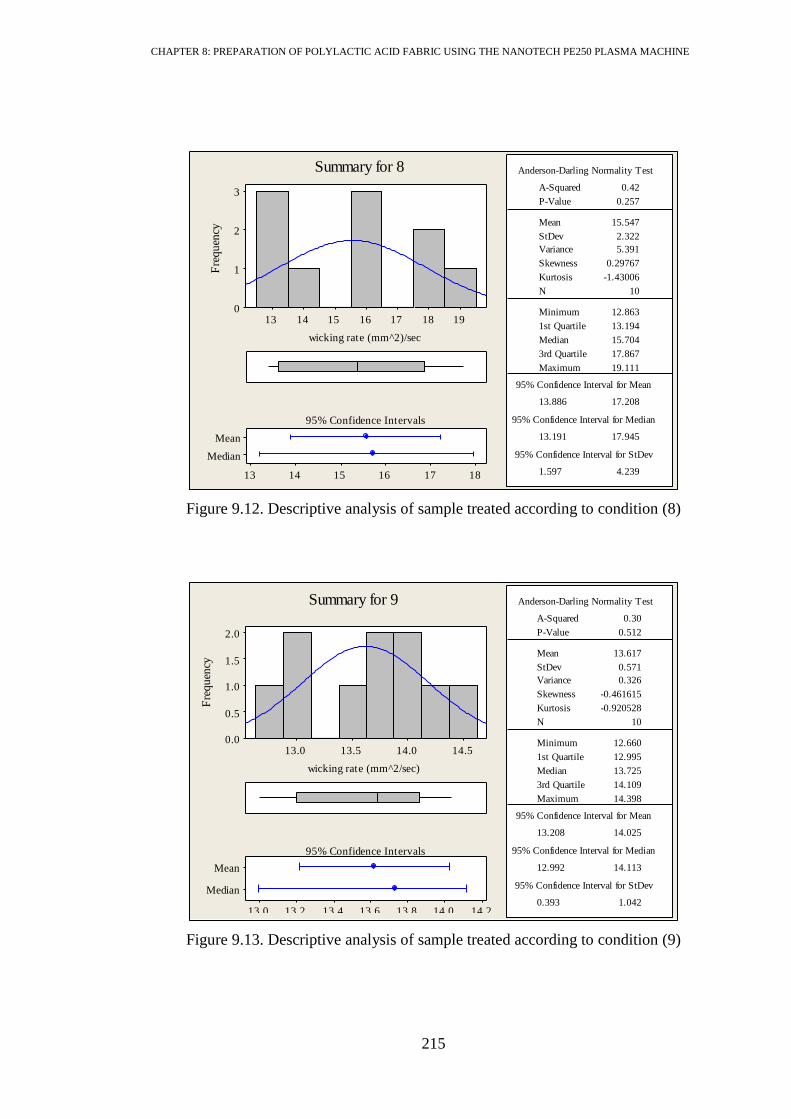
CHAPTER 8: PREPARATION OF POLYLACTIC ACID FABRIC USING THE NANOTECH PE250 PLASMA MACHINE
215
Figure 9.12. Descriptive analysis of sample treated according to condition (8)
Figure 9.13. Descriptive analysis of sample treated according to condition (9)
Median
Mean
181716151413
1st Quartile 13.194
Median 15.704
3rd Quartile 17.867
Maximum 19.111
13.886 17.208
13.191 17.945
1.597 4.239
A-Squared 0.42
P-Value 0.257
Mean 15.547
StDev 2.322
Variance 5.391
Skewness 0.29767
Kurtosis -1.43006
N 10
Minimum 12.863
Anderson-Darling Normality Test
95% Confidence Interval for Mean
95% Confidence Interval for Median
95% Confidence Interval for StDev
19181716151413
3
2
1
0
wicking rate (mm^2)/sec
Fre
qu
ency
95% Confidence Intervals
Summary for 8
Median
Mean
14.214.013.813.613.413.213.0
1st Quartile 12.995
Median 13.725
3rd Quartile 14.109
Maximum 14.398
13.208 14.025
12.992 14.113
0.393 1.042
A-Squared 0.30
P-Value 0.512
Mean 13.617
StDev 0.571
Variance 0.326
Skewness -0.461615
Kurtosis -0.920528
N 10
Minimum 12.660
Anderson-Darling Normality Test
95% Confidence Interval for Mean
95% Confidence Interval for Median
95% Confidence Interval for StDev
14.514.013.513.0
2.0
1.5
1.0
0.5
0.0
wicking rate (mm^2/sec)
Fre
qu
ency
95% Confidence Intervals
Summary for 9

CHAPTER 8: PREPARATION OF POLYLACTIC ACID FABRIC USING THE NANOTECH PE250 PLASMA MACHINE
216
Figure 9.14. Descriptive analysis of sample treated according to condition (10)
Figure 9.15. Descriptive analysis of sample treated according to condition (11)
21201918171615
3
2
1
0
wicking rate (mm^2/sec)
Fre
qu
ency
Median
Mean
19181716
1st Quartile 15.588
Median 16.851
3rd Quartile 19.158
Maximum 20.879
15.932 18.673
15.574 19.171
1.318 3.497
A-Squared 0.41
P-Value 0.270
Mean 17.303
StDev 1.916
Variance 3.670
Skewness 0.734474
Kurtosis -0.626759
N 10
Minimum 15.290
Anderson-Darling Normality Test
95% Confidence Interval for Mean
95% Confidence Interval for Median
95% Confidence Interval for StDev
95% Confidence Intervals
Summary for 10
Median
Mean
131211109
1st Quartile 8.988
Median 11.199
3rd Quartile 12.908
Maximum 15.447
8.958 12.901
8.890 13.088
1.896 5.032
A-Squared 0.17
P-Value 0.909
Mean 10.930
StDev 2.756
Variance 7.597
Skewness 0.101087
Kurtosis -0.390281
N 10
Minimum 6.425
Anderson-Darling Normality Test
95% Confidence Interval for Mean
95% Confidence Interval for Median
95% Confidence Interval for StDev
1614121086
wicking rate (mm^2/sec)
Fre
qu
en
cy
95% Confidence Intervals
Summary for 11

CHAPTER 8: PREPARATION OF POLYLACTIC ACID FABRIC USING THE NANOTECH PE250 PLASMA MACHINE
217
Figure 9.16. Descriptive analysis of sample treated according to condition (12)
9.2.1.2.2 Box Plot Representation of the Results
A box plot provides a convenient visual tool to compare the treated and control
substrates as demonstrated in Figure 9.17. Experimental conditions 1, 4, 5, 7, 10
resulted in wicking rates higher than the control one, whereas the conditions 2, 3, 6, 9,
11, 12 resulted in wicking rates less than the control one. Throughout the following
sections, the reasons for these results are suggested and discussed.
Two outliers (asterisked) appeared to deviate markedly from the observed values related
to experiments (4) and (7), which could be incorrect trials.
10987
wicking rate (mm^2/sec)
Fre
qu
en
cy
Median
Mean
9.08.58.07.5
1st Quartile 7.4692
Median 7.8046
3rd Quartile 8.6013
Maximum 9.9968
7.2959 8.8151
7.4682 8.7387
0.7304 1.9385
A-Squared 0.66
P-Value 0.058
Mean 8.0555
StDev 1.0618
Variance 1.1275
Skewness 0.840937
Kurtosis 0.595710
N 10
Minimum 6.4504
Anderson-Darling Normality Test
95% Confidence Interval for Mean
95% Confidence Interval for Median
95% Confidence Interval for StDev
95% Confidence Intervals
Summary for 12

CHAPTER 8: PREPARATION OF POLYLACTIC ACID FABRIC USING THE NANOTECH PE250 PLASMA MACHINE
218
Figure 9.17. Box plot of lipase treated PLA fabrics
9.2.1.2.3 Statistical Comparison of Control and Treated Samples
This statistical comparison, using Levene and t-tests, which were introduced in Chapter
5, was used to reveal if the means of the wicking rates after enzyme treatment were
statistically different from the control mean. The results of Levene and t-tests are
presented in Table 9.5.
The Levene test showed that treatment conditions 3, 4, 5, 6, 7, 8, 10, 11, 12 had equal
variances as the control fabric, because the probability values P were larger than the
pre-chosen significance level α = 0.05. On the other hand, the t-test proved that all
treatment conditions (except 8 and 9) achieved statistically different wicking rates from
the control one because the probability values P were smaller than the pre-chosen
significance level 0.05.
121110987654321C
22.5
20.0
17.5
15.0
12.5
10.0
7.5
5.0
Experiment
wic
kin
g r
ate
(m
m^2
/sec)
14.82
control PLA

CHAPTER 8: PREPARATION OF POLYLACTIC ACID FABRIC USING THE NANOTECH PE250 PLASMA MACHINE
219
Table 9.5. Levene and t-test results of the wicking rates data
experiment Time (hour) Concentration (ml) pH Levene test t-test
1 1 0.5 5 0.012 0.000
2 1 0.5 7 0.019 0.006
3 1 0.5 8 0.232 0.004
4 1 1 5 0.788 0.001
5 1 1 7 0.096 0.000
6 1 1 8 0.336 0.000
7 3 0.5 5 0.173 0.000
8 3 0.5 7 0.398 0.440
9 3 0.5 8 0.003 0.061
10 3 1 5 0.814 0.007
11 3 1 7 0.285 0.002
12 3 1 8 0.057 0.000
9.2.1.2.4 Interaction Plot
An interaction plot creates a single interaction plot for two factors, or a matrix of
interaction plots for three to nine factors. An interaction plot is a plot of means for each
level of a factor, with the level of a second factor held constant. Interaction plots are
useful for judging the presence of interaction.
Interaction is present when the response at a factor level depends upon the level(s) of
other factors. Parallel lines in an interaction plot indicate no interaction. The greater the
departure of the lines from the parallel state, the higher the degree of interaction. Each
point on the graph represents the mean score of a combination of conditions.
Figure 9.18 demonstrates the interactions between the enzymatic preparation
parameters. The plots revealed that the (time – pH) and (time – concentration)
interactions were very small. On the other hand, the (concentration – pH) interaction
was more pronounced, in particular at pH 7, where two opposite behaviours were
detected. At pH 7 the wicking rate increased with increasing concentration, whereas at
pH 8 the wicking rate decreased with increasing concentration.

CHAPTER 8: PREPARATION OF POLYLACTIC ACID FABRIC USING THE NANOTECH PE250 PLASMA MACHINE
220
Figure 9.18. Full matrix of interaction plots (the transpose of each plot in the upper right
displays in the lower left portion of the matrix)
9.2.1.2.5 Regression Model of Wicking Rate with Time, Concentration, pH
General linear multiple regression was run to produce an equation that could predict the
value of a dependant variable (W) using the independent variables pH, time, and
concentration.
Initial Regression
The regression equation is:
W = 35.0 - 0.114 time - 3.01 concentration - 2.75 pH Equation 9.1
where the units of the time and concentration is seconds and millimetre respectively
The analysis of variance of the regression model is shown in Table 9.6. The probability
value P is smaller than the pre-selected significance level α = 0.05 proving there is
strong linear relationship between the independent and dependant variables at the 95%
confidence level.
20
15
10
875
1.00.5
20
15
10
31
20
15
10
time
concentration
pH
1
3
time
0.5
1.0
concentration
5
7
8
pH
Interaction Plot for WData Means

CHAPTER 8: PREPARATION OF POLYLACTIC ACID FABRIC USING THE NANOTECH PE250 PLASMA MACHINE
221
The detailed analysis of the regression model is shown in Table 9.7. R-sq = 72.2%
indicated that 72.2% of the variation in the independent variable (W) is explained by the
regression model (Equation 9.1).
The probability P-values of the pH and the constant were found to be (0.002) and
(0.000) respectively. They are smaller than the pre-chosen significance level (α = 0.05)
for this research (Chapter 5). So the pH and constant are real effective values in this
model at 95% confidence.
The probability P-values of the concentration and time were (0.357) and (0.886)
respectively, higher than the significance level. Physically these parameters cannot be
ignored, statistically it could be considered less significant, at confident level 64.3 %
and 11.4 % for concentration and time respectively. In other words, it can be concluded
that there was no need for prolonged treatment or higher concentration because the
enzyme can etch the amorphous in small time and little amount of enzyme will be
enough to occupy all possible function sites on the substrate surface.
Table 9.6. Analysis of variance
Source DF SS MS F P
Regression 3 148.264 49.421 6.92 0.013
Residual Error 8 57.124 7.140
Total 11 205.388
Table 9.7. Detailed analysis of regression model
Predictor Coef Se Coef P
Constant 4.992 5.033 0.000
time -0.1138 0.7714 0.886
concentration -3.015 3.086 0.357
pH -2.7512 0.6185 0.002
S = 2.67216 R-Sq = 72.2% R-Sq(adj) = 61.8%

CHAPTER 8: PREPARATION OF POLYLACTIC ACID FABRIC USING THE NANOTECH PE250 PLASMA MACHINE
222
9.2.2 Buffer Treatment
Various workers have investigated the effect of processing media on the properties of
PLA fabric. This was correlated with pH level and degradation mechanism. It was
claimed that PLA undergoes bulk degradation (over the cross-section of substrate)
under acidic and neutral pH conditions [202, 203], whereas surface erosion occurred
under alkaline conditions [204].
Jantip [205] observed the effects of pH values of dyeing liquors on the properties of
PLA. It was found that dyeing PLA fabric under neutral conditions resulted in a more
dramatic loss in molecular weight than when the dyeing was carried out for the same
length of time under acidic conditions (pH 5). It was observed also that the pH value of
the dyeing liquor dropped when the PLA fabric was dyed at 120°C under neutral
conditions, especially for longer times of processing (120 min). This might be due to the
formation of carboxylic acid residues (lactic acid and lactic acid oligomers) as a
degradation product during processing.
It was found that hydrolytic degradation caused the cleavage of ester groups, resulting
in an increased number of hydrophilic terminal groups (hydroxyl and carboxyl groups).
Therefore the surface hydrophilicity of PLA-based materials increased as shown in
Figure 9.19, due to change in the advancing contact angle during alkaline hydrolytic
degradation or enzymatic degradation [206].

CHAPTER 8: PREPARATION OF POLYLACTIC ACID FABRIC USING THE NANOTECH PE250 PLASMA MACHINE
223
Figure 9.19. Contact angle change during alkaline hydrolytic degradation and enzymatic
degradation [206]
The following section investigated the effect of processing media on PLA fabric. The
samples were treated in buffer solution “without enzyme” under the same conditions
used for the enzyme preparation process. This investigation would help in
understanding the real effect of the enzyme on the modifications detected on the PLA
fabric.
9.2.2.1 Experiment and Procedure
The buffer treatment experiments included two parameters, time at the two levels of 1
and 3 hours, and pH at the three levels 5.5, 7 and 8. The design of the experiment is
presented in Table 9.8. Practically the experiments were run in random order to lessen
the effects of variation caused by any external factors that were not included in the
study. The results were presented in the standard order shown in Table 9.8.
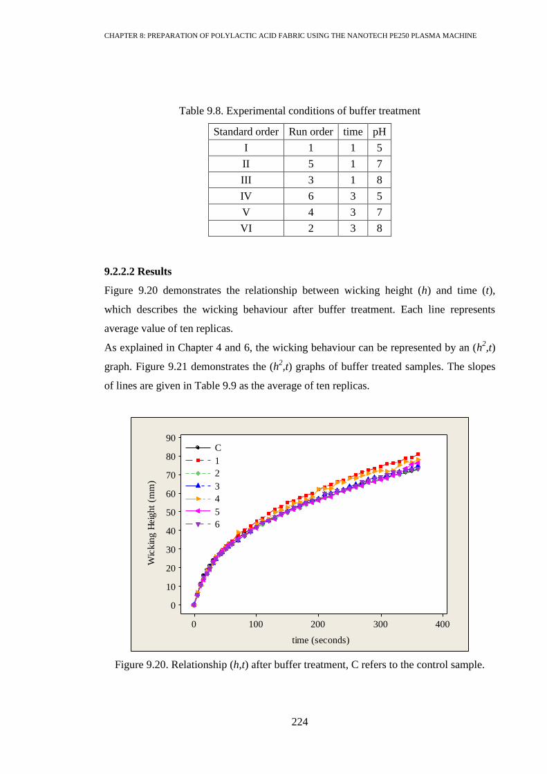
CHAPTER 8: PREPARATION OF POLYLACTIC ACID FABRIC USING THE NANOTECH PE250 PLASMA MACHINE
224
Table 9.8. Experimental conditions of buffer treatment
Standard order Run order time pH
I 1 1 5
II 5 1 7
III 3 1 8
IV 6 3 5
V 4 3 7
VI 2 3 8
9.2.2.2 Results
Figure 9.20 demonstrates the relationship between wicking height (h) and time (t),
which describes the wicking behaviour after buffer treatment. Each line represents
average value of ten replicas.
As explained in Chapter 4 and 6, the wicking behaviour can be represented by an (h2,t)
graph. Figure 9.21 demonstrates the (h2,t) graphs of buffer treated samples. The slopes
of lines are given in Table 9.9 as the average of ten replicas.
Figure 9.20. Relationship (h,t) after buffer treatment, C refers to the control sample.
4003002001000
90
80
70
60
50
40
30
20
10
0
time (seconds)
Wic
kin
g H
eig
ht
(mm
)
C
1
2
3
4
5
6

CHAPTER 8: PREPARATION OF POLYLACTIC ACID FABRIC USING THE NANOTECH PE250 PLASMA MACHINE
225
Figure 9.21. (h2,t) graphs of buffer treated samples
Table 9.9. Wicking rates (mm2/sec) of buffer treated samples
run 1 2 3 4 5 6 7 8 9 10 Average
I 17.13 17.26 18.94 20.11 17.68 17.60 19.10 19.12 19.13 18.00 18.41
II 15.92 12.33 13.58 12.28 11.66 19.07 18.82 17.68 15.00 14.20 15.05
III 16.48 14.36 15.24 15.18 16.86 14.00 14.20 16.10 15.30 16.40 15.41
IV 16.14 14.61 16.00 17.13 17.26 18.94 20.11 17.68 17.60 19.10 17.46
V 15.92 12.33 13.58 12.28 11.66 19.07 18.82 17.68 13.00 17.50 15.18
VI 16.48 14.36 15.24 15.18 16.86 17.00 15.30 14.00 13.70 14.30 15.24
9.2.2.3 Statistical Analysis
The following analysis provides descriptive statistics of the buffer treatment
experiments and comparisons between enzyme and buffer treatments of PLA fabric
using the Levene and t-tests.
9.2.2.3.1 Descriptive Analysis
The descriptive analysis gives detailed information about each experiment including
mean, standard deviation and normal distribution. Each treatment condition was
repeated ten times, and tested for wicking behaviour.
4003002001000
7000
6000
5000
4000
3000
2000
1000
0
time (seconds)
H^2
(m
m^2
)C
1
2
3
4
5
6

CHAPTER 8: PREPARATION OF POLYLACTIC ACID FABRIC USING THE NANOTECH PE250 PLASMA MACHINE
226
The following graphical illustrations are the descriptive analyses of experimental
conditions I, II, III, IV, V, VI.
The results proved that the data of each experiment were normally distributed as the P-
values for the Anderson-Darling Normality test were higher than the pre-selected
significance level (α = 0.05) of this project.
The experiments II, III, V, VI gave average values of wicking rates in the vicinity of the
control wicking rate, whereas the mean values of I and IV was higher than that of the
control.
Figure 9.22. Descriptive analysis of experiment I
Median
Mean
19.0018.7518.5018.2518.0017.7517.50
1st Quartile 17.513
Median 18.470
3rd Quartile 19.126
Maximum 20.112
17.692 19.123
0.688 1.825
A-Squared 0.45
P-Value 0.221
Mean 18.408
StDev 1.000
Variance 1.000
Skewness 0.22202
Kurtosis -1.18993
N 10
Minimum 17.130
Anderson-Darling Normality Test
95% Confidence Interval for Mean
95% Confidence Interval for StDev
20.019.519.018.518.017.517.0
4
3
2
1
0
wicking rate (mm^2/sec)
Fre
qu
en
cy
95% Confidence Intervals
Summary for I

CHAPTER 8: PREPARATION OF POLYLACTIC ACID FABRIC USING THE NANOTECH PE250 PLASMA MACHINE
227
Figure 9.23. Descriptive analysis of experiment II
Figure 9.24. Descriptive analysis of experiment III
18161412
3
2
1
0
wicking rate (mm^2/sec)
Fre
qu
en
cy
Median
Mean
18171615141312
1st Quartile 12.317
Median 14.600
3rd Quartile 17.963
Maximum 19.073
13.095 17.013
1.884 4.999
A-Squared 0.32
P-Value 0.470
Mean 15.054
StDev 2.739
Variance 7.500
Skewness 0.35497
Kurtosis -1.38520
N 10
Minimum 11.663
Anderson-Darling Normality Test
95% Confidence Interval for Mean
95% Confidence Interval for StDev
95% Confidence Intervals
Summary for II
Median
Mean
16.516.015.515.014.514.0
1st Quartile 14.323
Median 15.270
3rd Quartile 16.420
Maximum 16.864
14.683 16.142
0.701 1.861
A-Squared 0.33
P-Value 0.455
Mean 15.413
StDev 1.020
Variance 1.040
Skewness -0.02880
Kurtosis -1.45787
N 10
Minimum 14.000
Anderson-Darling Normality Test
95% Confidence Interval for Mean
95% Confidence Interval for StDev
17.016.516.015.515.014.514.0
wicking rate (mm^2/sec)
Fre
qu
ency
95% Confidence Intervals
Summary for III

CHAPTER 8: PREPARATION OF POLYLACTIC ACID FABRIC USING THE NANOTECH PE250 PLASMA MACHINE
228
Figure 9.25. Descriptive analysis of experiment IV
Figure 9.26. Descriptive analysis of experiment V
201918171615
2.4
1.8
1.2
0.6
0.0
wicking rate (mm^2/sec)
Fre
qu
en
cy
Median
Mean
19.018.518.017.517.016.516.0
1st Quartile 16.105
Median 17.428
3rd Quartile 18.979
Maximum 20.112
16.285 18.628
1.126 2.990
A-Squared 0.18
P-Value 0.879
Mean 17.457
StDev 1.638
Variance 2.682
Skewness -0.067748
Kurtosis -0.234846
N 10
Minimum 14.607
Anderson-Darling Normality Test
95% Confidence Interval for Mean
95% Confidence Interval for StDev
95% Confidence Intervals
Summary for IV
18161412
3
2
1
0
wicking rate (mm^2/sec)
Fre
qu
en
cy
Median
Mean
18171615141312
1st Quartile 12.317
Median 14.749
3rd Quartile 17.963
Maximum 19.073
13.094 17.273
12.312 18.068
2.009 5.333
A-Squared 0.53
P-Value 0.128
Mean 15.184
StDev 2.921
Variance 8.533
Skewness 0.16224
Kurtosis -1.96709
N 10
Minimum 11.663
Anderson-Darling Normality Test
95% Confidence Interval for Mean
95% Confidence Interval for Median
95% Confidence Interval for StDev
95% Confidence Intervals
Summary for V

CHAPTER 8: PREPARATION OF POLYLACTIC ACID FABRIC USING THE NANOTECH PE250 PLASMA MACHINE
229
Figure 9.27. Descriptive analysis of experiment VI
9.2.2.3.2 Statistical Comparison between Buffer Treated and Enzyme Treated
Samples
Each buffer treated experiment was compared with its opposite number of the enzyme
treated experiments, which was subjected to the same conditions of pH and time. The
results of wicking rates obtained after buffer treatment are given in
Table 9.9 and were compared with the wicking rate results obtained after enzyme
treatment and given in Table 9.4. The Levene test compared the variances of the buffer
treated samples with the enzyme treated samples. The results are shown in Table 9.10.
Two cases (II - 5) and (III - 6) were found to reject the null hypothesis of equal
variances because the P-values were smaller than the significance level of α = 0.05. This
means that the groups (II - 5) and (III - 6) had unequal variances and should be
considered as unpaired samples when applying the t-test.
17161514
2.0
1.5
1.0
0.5
0.0
wicking rate (mm^2/sec)
Fre
qu
en
cy
Median
Mean
16.516.015.515.014.514.0
1st Quartile 14.225
Median 15.210
3rd Quartile 16.576
Maximum 17.000
14.388 16.097
0.822 2.181
A-Squared 0.39
P-Value 0.317
Mean 15.243
StDev 1.194
Variance 1.427
Skewness 0.36438
Kurtosis -1.31324
N 10
Minimum 13.700
Anderson-Darling Normality Test
95% Confidence Interval for Mean
95% Confidence Interval for StDev
95% Confidence Intervals
Summary for VI
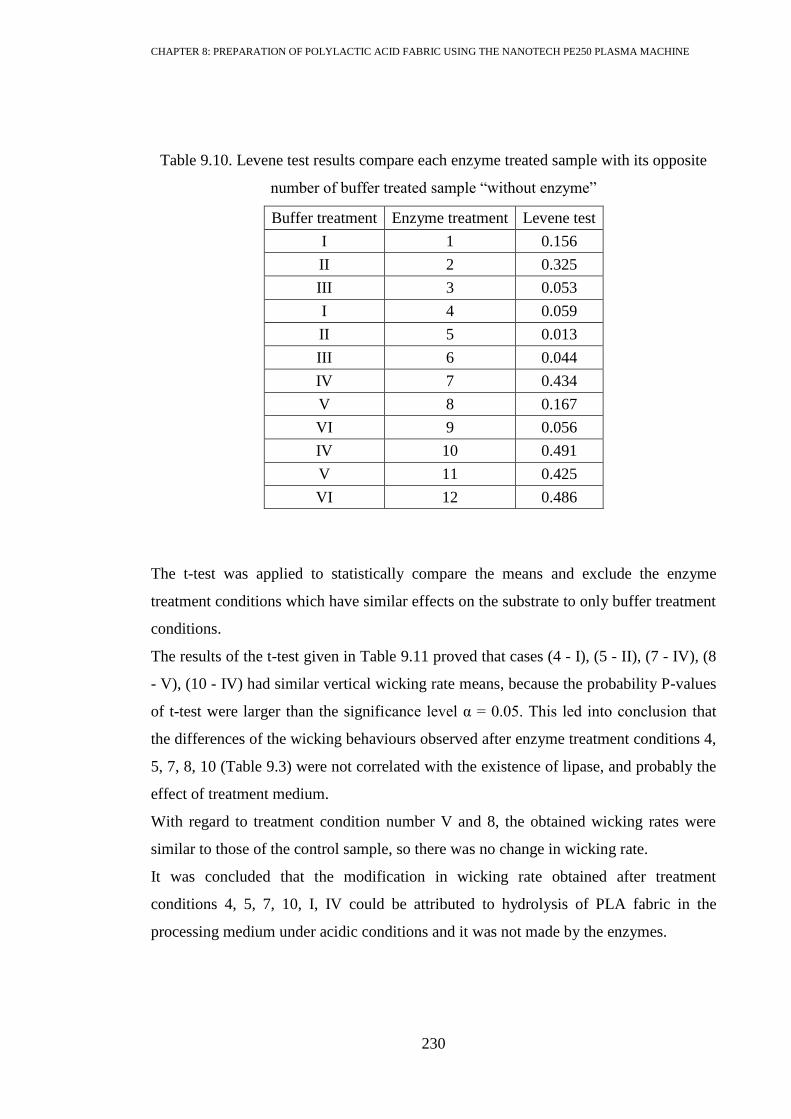
CHAPTER 8: PREPARATION OF POLYLACTIC ACID FABRIC USING THE NANOTECH PE250 PLASMA MACHINE
230
Table 9.10. Levene test results compare each enzyme treated sample with its opposite
number of buffer treated sample “without enzyme”
Buffer treatment Enzyme treatment Levene test
I 1 0.156
II 2 0.325
III 3 0.053
I 4 0.059
II 5 0.013
III 6 0.044
IV 7 0.434
V 8 0.167
VI 9 0.056
IV 10 0.491
V 11 0.425
VI 12 0.486
The t-test was applied to statistically compare the means and exclude the enzyme
treatment conditions which have similar effects on the substrate to only buffer treatment
conditions.
The results of the t-test given in Table 9.11 proved that cases (4 - I), (5 - II), (7 - IV), (8
- V), (10 - IV) had similar vertical wicking rate means, because the probability P-values
of t-test were larger than the significance level α = 0.05. This led into conclusion that
the differences of the wicking behaviours observed after enzyme treatment conditions 4,
5, 7, 8, 10 (Table 9.3) were not correlated with the existence of lipase, and probably the
effect of treatment medium.
With regard to treatment condition number V and 8, the obtained wicking rates were
similar to those of the control sample, so there was no change in wicking rate.
It was concluded that the modification in wicking rate obtained after treatment
conditions 4, 5, 7, 10, I, IV could be attributed to hydrolysis of PLA fabric in the
processing medium under acidic conditions and it was not made by the enzymes.

CHAPTER 8: PREPARATION OF POLYLACTIC ACID FABRIC USING THE NANOTECH PE250 PLASMA MACHINE
231
Table 9.11. t-test results compare each enzyme treated sample with its opposite number
of buffer treated sample “without enzyme”
Buffer treatment Enzyme treatment t-test
I 1 0.000
II 2 0.007
III 3 0.002
I 4 0.519
II 5 0.060
III 6 0.000
IV 7 0.051
V 8 0.762
VI 9 0.002
IV 10 0.849
V 11 0.004
VI 12 0.000
9.2.3 XPS Analysis of Surface Chemical Composition
The previous discussion of the wicking rate data proved that the experimental
conditions numbers 4, 5, 7, 8 and 10 were statistically the same as the buffer treated
samples. Also it proved that the experimental condition 9 appeared to give no difference
in the wicking rate from that of the control sample.
The interest of this analysis was to study the enzyme effects on the surface chemistry of
the substrate. Seven groups of the enzyme experimental conditions (1, 2, 3, 6, 11, 12)
exhibited an effect on the substrates. Out of these seven samples, two groups (1) and
(12) with the most effect on the average wicking rate and least standard deviation were
selected to be investigated by the XPS technique. The XPS scan of control PLA was
introduced in Chapter 6.
The highest average wicking rate was detected after lipase treatment condition number
(1) as presented in Table 9.4. The XPS survey scan of this sample is shown in Figure
9.28, and the relative chemical composition is given in Table 9.12.
Since enzyme treated sample (1) showed no change in the chemical composition of the
substrate, it was thought that the increase in the wicking rate after this treatment could

CHAPTER 8: PREPARATION OF POLYLACTIC ACID FABRIC USING THE NANOTECH PE250 PLASMA MACHINE
232
be attributed to roughing of the fibre surface, due to enzyme hydrolysis, which was
demonstrated later by the SEM images in Section (9.3.6).
Figure 9.28. Survey scan of enzyme treated sample (1)
In contrast, the lowest wicking rate was found after enzyme preparation number (12).
The survey scan of this sample is illustrated in Figure 9.29, where a nitrogen peak was
detected at 400 (eV), as well as the increase in the relative nitrogen percentage
presented in Table 9.12. The nitrogen was formed on the surface from the residual
lipase. This could explain the decline in wicking rate of PLA fabric after enzyme
treatment, as the testing liquid may be absorbed by the nitrogenous material.
In order to help explaining the role of enzyme in producing this nitrogen on the surface,
buffer treated sample IV (Table 9.8) was examined by XPS.
Figure 9.30 presents the survey scan of the buffer treated samples, and the relative
chemical composition is given in Table 9.12. The XPS analysis appeared similar to that
of the control PLA, which indicated that the increase in wicking rate found in this case
could be attribute to the surface etching by acidic hydrolysis, as appeared in the SEM
scan.
0
20,000
40,000
60,000
80,000
100,000
120,000
200 400 600 800 1,000 1,200 1,400
count
per
sec
ond
Binding Energy (eV)
C1s
O1s

CHAPTER 8: PREPARATION OF POLYLACTIC ACID FABRIC USING THE NANOTECH PE250 PLASMA MACHINE
233
Figure 9.29. Survey scan of enzyme treated sample (12)
Figure 9.30. Survey scan of buffer treated sample (IV)
0
20,000
40,000
60,000
80,000
100,000
120,000
200 400 600 800 1,000 1,200 1,400
count
per
sec
ond
Binding Energy (eV)
O1s
C1s
N1s
0
20,000
40,000
60,000
80,000
100,000
120,000
200 400 600 800 1,000 1,200 1,400
count
per
sec
ond
Binding Energy (eV)
C1s
O1s

CHAPTER 8: PREPARATION OF POLYLACTIC ACID FABRIC USING THE NANOTECH PE250 PLASMA MACHINE
234
Table 9.12. Relative element composition
Sample Identifier C 1s % N 1s % O 1s % N/C% O/C%
PLA control 64.70 0.22 35.10 0.34 54.22
Experiment condition (1) 66.98 1.16 31.86 1.73 47.56
Experiment condition (12) 67.37 4.54 28.09 6.74 41.69
Experiment condition (IV) 65.97 0.92 33.11 1.39 50.20
9.2.4 Scanning Electron Microscopy (SEM)
9.2.4.1 SEM Images of Control PLA Fibre
The SEM micrographs shown in Figure 9.31, Figure 9.32, Figure 9.33 illustrate the
surface of the control PLA fibre. It appeared to be generally smooth with some random
blisters and ripples running parallel and perpendicular to the fibre length; these were
made by the production process.
Figure 9.31. SEM micrograph of control PLA fibre

CHAPTER 8: PREPARATION OF POLYLACTIC ACID FABRIC USING THE NANOTECH PE250 PLASMA MACHINE
235
Figure 9.32. SEM micrograph of control PLA fibre
Figure 9.33. SEM micrograph of control PLA fibre

CHAPTER 8: PREPARATION OF POLYLACTIC ACID FABRIC USING THE NANOTECH PE250 PLASMA MACHINE
236
9.2.4.2 SEM Images of Lipase Treated Samples
Damage and change in surface topography was detected by SEM analysis after the
lipase preparation. The effects were random and not localised to any particular area of
the fibre. Blisters in form of clusters accumulated on the surface randomly, as illustrated
in Figure 9.34 and Figure 9.35, which are believed to be residual lipase adhering to the
fabric surface resulting from the preparation process under conditions (11) and (12).
Voids and cracks can also be seen in the SEM micrographs as shown in Figures 9.38 -
40, which could be produced by lipase and buffer hydrolysis, in addition to the
mechanical action by the physical agitation inside the treatment bath. These features
were noticed when the samples were treated under enzyme conditions (1), and
sometimes under the buffer treated samples given in Table 9.3 and Table 9.8
respectively.
The samples treated under treatment condition (1) exhibited higher roughness and more
etching places which indicated that the lipase worked in this condition and caused
surface hydrolysis that led to wicking rate increase.
Figure 9.34. SEM micrograph of sample treated under condition (11)
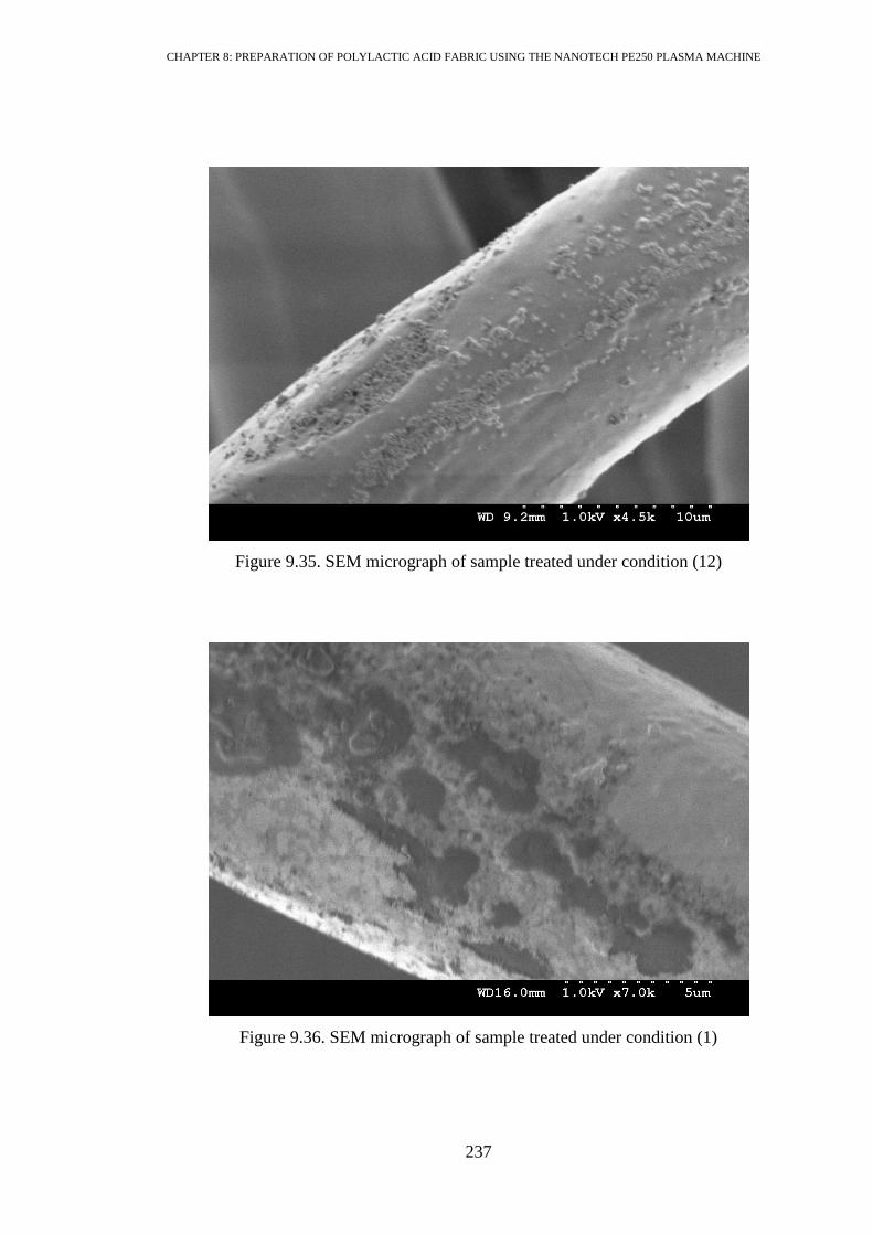
CHAPTER 8: PREPARATION OF POLYLACTIC ACID FABRIC USING THE NANOTECH PE250 PLASMA MACHINE
237
Figure 9.35. SEM micrograph of sample treated under condition (12)
Figure 9.36. SEM micrograph of sample treated under condition (1)
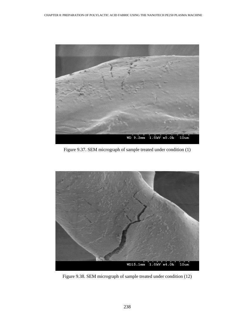
CHAPTER 8: PREPARATION OF POLYLACTIC ACID FABRIC USING THE NANOTECH PE250 PLASMA MACHINE
238
Figure 9.37. SEM micrograph of sample treated under condition (1)
Figure 9.38. SEM micrograph of sample treated under condition (12)

CHAPTER 8: PREPARATION OF POLYLACTIC ACID FABRIC USING THE NANOTECH PE250 PLASMA MACHINE
239
Figure 9.39. SEM micrograph of sample treated under condition (I)
9.3 Protease Wash
The effective removal of residual protein from the fabric is important for further
processing. Various methods have been applied to achieve complete removal of the
enzyme protein adhering to the surface. In a study by Brueckner [207], the enzymatic
treated samples were washed with Triton X-100 (5 g/l) and subsequently with Na2CO3
(2 g/l) for 30 min at 50°C, further with deionised water for 30 min and additionally
soxhlet extracted overnight with ethanol and rinsed in pure water to remove the
adsorbed protein. Other researchers used protease enzyme to hydrolyze the protein [208,
209].
In view of the XPS results, the enzyme treatment condition (12), which resulted in high
level of nitrogen over the substrate, was subjected to a protease wash, then rinsed with
normal running water for 10 minutes, then washed at 60ºC for 15min using (2g/l)
sodium carbonate and (1g/l) Synperonic detergent. Further it was rinsed with distilled
water and left to dry at room temperature.
Proteases from bacillus licheniformis with activity unit 2.4 AU/g, was used for the
washing process. The protease washing procedure is shown in Figure 9.40. The liquor
to goods ratio was 15:1.

CHAPTER 8: PREPARATION OF POLYLACTIC ACID FABRIC USING THE NANOTECH PE250 PLASMA MACHINE
240
This test was repeated ten times. Figure 9.41 illustrates the descriptive analysis for ten
replicas. The Levene and t-test results are shown in Table 9.13, it was found that
statistically there was no difference between the control and protease washed samples in
regard to the variances and means, because the probability values P were higher than the
significance value α = 0.05.
It was concluded that the decrease in wicking rate found after enzyme preparation
(Table 9.4) was due to absorption of the wicking liquid by the residual protein adhering
to the surface of the substrate.
80°C, 10min
60°C, 30min, pH8
Cooling as quickly as possible
Heating as quickly as possible
Figure 9.40. Protease washing procedure

CHAPTER 8: PREPARATION OF POLYLACTIC ACID FABRIC USING THE NANOTECH PE250 PLASMA MACHINE
241
Figure 9.41. Descriptive statistics of ten samples treated by enzyme then washed by
protease, *refers to outlier point
Table 9.13. Statistical comparison between sample treated by lipase then washed by
protease and control sample
Experiment Levene test t-test
Protease wash 0.302 0.571
9.4 Further Attempts to Improve Wicking Rate
Further attempts were investigated using different enzymes to try to improve the
wicking rate by enzyme treatments. The volume of the processing tube in which the
fabric was dipped to be treated by enzyme was reduced in order to keep the enzymes in
contact with the substrate, but there was no difference from the previously reported
results. Also the speed of rotation was increased with the purpose of increasing the
agitation which could provide more interaction between the enzyme and the fabric, but
it was not successful in achieving any noticeable difference. The processing temperature
of the enzyme preparation also was altered to different values (70°C and 45°C), but the
18171615141312
wicking rate (mm^2/sec)
Fre
quency
Median
Mean
15.515.014.514.013.513.0
1st Quartile 13.299
Median 14.397
3rd Quartile 14.625
Maximum 18.409
13.225 15.559
1.122 2.979
A-Squared 0.91
P-Value 0.012
Mean 14.392
StDev 1.632
Variance 2.663
Skewness 1.62284
Kurtosis 4.51730
N 10
Minimum 12.209
Anderson-Darling Normality Test
95% Confidence Interval for Mean
95% Confidence Interval for StDev
95% Confidence Intervals

CHAPTER 8: PREPARATION OF POLYLACTIC ACID FABRIC USING THE NANOTECH PE250 PLASMA MACHINE
242
obtained wicking rates were in the vicinity of what was found at 60°C. Enzyme
concentration was changed, but it did not achieve noticeable difference in comparison
with the findings reported before.
It seemed that this enzyme had limited effect on the PLA, and any effect it had was
mainly concentrated at the surface. It could be because the enzyme molecule is large
and not able to access the pores of the fabric.
9.5 Dye Application
Dyeing processes were applied to examine how the previous preparation processes may
affect the applications of PLA fabric. Dyeing experiments were applied to the treated
samples which exhibited the highest modifications in wicking rate values, which were
experiment conditions (1) and (12).
Disperse dye red C.I 60 B-2B 200 % and acid dye C.I Acid Blue 25 were applied. The
disperse dye is usually the common application class for dyeing PLA. The attempt of
using an acid dye was made to evaluate whether the nitrogen content found on the
substrate after the enzyme treatment would be effective in producing positively charged
polar groups that could attract the anionic dyes (negative charge).
9.5.1 Disperse Dye The dyeing process was as that used for the control PLA fabric, given in Section 6.5.
Colour Measurement
The visual colour yields, expressed by the K/S values, were measured twice, before and
after the wash fastness test. The higher the K/S value, the greater is the colour intensity
and, hence, the better is the dye uptake for a given fabric and dye.
The spectral reflectance values (400-700 nm) were measured using a Spectra Flash
SF600 spectrophotometer (Datacolor International) using 9.00 mm aperture.
Figure 9.42 shows the colour yields of treated fabric under condition (1) and compared
with control sample. As can be seen the graphs nearly coincide, which indicates that this
enzyme preparation condition did not modify the dyeing behaviour, though
modification in wicking rate was detected.
Also, the sample treated under condition (12) did not exhibit major differences from the
control one, as can be seen in the Figure 9.43.

CHAPTER 8: PREPARATION OF POLYLACTIC ACID FABRIC USING THE NANOTECH PE250 PLASMA MACHINE
243
It can be concluded that the application of the disperse dye to the fabric treated with
Lipase 76 did not produce any considerable improvement in colour yield; it could be
because the enzyme effect was slightly surface etching.
Figure 9.42. Colour measurement of PLA treated under condition (1)
0
1
2
3
4
5
6
7
8
400 450 500 550 600 650 700 750
K/S
Wavelength (nm)
PLA untreated disperse 3% before
wash fastness test
PLA untreated disperse 3% after wash
fastness test
PLA treated 76 pH5 disperse 3% before
wash fastness test
PLA treated 76 pH5 disperse 3% after
wash fastness test
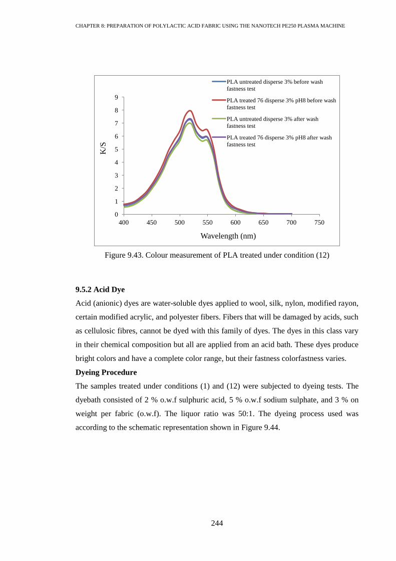
CHAPTER 8: PREPARATION OF POLYLACTIC ACID FABRIC USING THE NANOTECH PE250 PLASMA MACHINE
244
Figure 9.43. Colour measurement of PLA treated under condition (12)
9.5.2 Acid Dye
Acid (anionic) dyes are water-soluble dyes applied to wool, silk, nylon, modified rayon,
certain modified acrylic, and polyester fibers. Fibers that will be damaged by acids, such
as cellulosic fibres, cannot be dyed with this family of dyes. The dyes in this class vary
in their chemical composition but all are applied from an acid bath. These dyes produce
bright colors and have a complete color range, but their fastness colorfastness varies.
Dyeing Procedure
The samples treated under conditions (1) and (12) were subjected to dyeing tests. The
dyebath consisted of 2 % o.w.f sulphuric acid, 5 % o.w.f sodium sulphate, and 3 % on
weight per fabric (o.w.f). The liquor ratio was 50:1. The dyeing process used was
according to the schematic representation shown in Figure 9.44.
0
1
2
3
4
5
6
7
8
9
400 450 500 550 600 650 700 750
K/S
Wavelength (nm)
PLA untreated disperse 3% before wash
fastness test
PLA treated 76 disperse 3% pH8 before wash
fastness test
PLA untreated disperse 3% after wash
fastness test
PLA treated 76 disperse 3% pH8 after wash
fastness test

CHAPTER 8: PREPARATION OF POLYLACTIC ACID FABRIC USING THE NANOTECH PE250 PLASMA MACHINE
245
100C for 30min
Heating 2C/min up to 100ºC
Cooling as quickly as possible to 40ºC
40ºC for ten minutes
Heating as quickly as possible up to 40ºC
Figure 9.44. Schematic representation of dyeing process by acid dye
Colour Measurement
With regard to the sample treated under condition (1), clearly it could not be dyed by
acid dye as the control PLA fabric, as can been from the K/S graph shown in Figure
9.45. This result was expected because this preparation condition did not produce any
polar groups on the surface.
The sample treated under condition (12) exhibited different dyeing behaviour from
control sample. Figure 9.46 illustrates the K/S graph of control and treated samples
before and after wash fastness test. The treated sample seemed to absorb some dye as
indicated by the higher colour yield from the control, exhibited on the K/S graph.
However the colour yield decreased after wash fastness test.
This dyeing behaviour indicated that the nitrogen detected on the surface could help in
absorbing the dye, but it was not chemically effective to help bonding the dye to the
fabric. Its effect was not permanent.
It can be concluded that lipase 76 has very little effect on the surface of PLA fabric
mostly appeared after treatment condition number (1), whereas other treatment
condition led to some adsorption of residual enzymes on the surface.

CHAPTER 8: PREPARATION OF POLYLACTIC ACID FABRIC USING THE NANOTECH PE250 PLASMA MACHINE
246
Figure 9.45. Colour measurement of PLA fabric treated under condition (1)
Figure 9.46. Colour measurement of PLA fabric treated under condition number (12)
0
0.02
0.04
0.06
0.08
0.1
0.12
0.14
0.16
0.18
400 450 500 550 600 650 700 750
K/S
Wavelength (nm)
PLA untreated
PLA treated with condition (1)
0
0.2
0.4
0.6
0.8
1
1.2
400 450 500 550 600 650 700 750
K/S
Wavelength (nm)
treated before wash test
treated after wash test
nontreated before wash test
nontreated after wash test

CHAPTER 10: CONCLUSION, RECOMMENDATION AND FUTURE WORK
247
Chapter 10
CONCLUSIONS AND RECOMMENDATIONS FOR FUTURE WORK
10.1 Conclusions
10.1.1 Aim 1 - Investigate the Liquid Transport through poly(lactic acid) Fabric
The study of liquid transport behaviour was chosen first because of the need to establish
the fundamental facts of the ability of PLA fabric to transport liquid, secondly due to
the common existence of liquid-fibre interactions in textile processing.
The results were used to set out a comparable evaluation between substrates before and
after enzyme and plasma preparations to determine their effects on fabric properties.
The statistical analysis proved that the vertical wicking through PLA knitted fabric is
linear and can be described by linear numerical model at accuracy of 99.6% of
representing the change of wicking height with time. Also the study showed that the
period of observing the vertical wicking to calculate the wicking rate when studying
textile materials should be reported along with wicking rate value because of building
the hydrostatic pressure.
With regard to spreading of micro-drops, a device was developed for evaluating the
spreading behaviour, with effective implementation for image analysis.
The experimental work showed that the spreading of liquid through PLA fabric consists
of two phases. Statistical analysis proved that each phase can be represented by linear
models.
A comparison between PLA knitted fabric and woven PET fabric given in Chapter 7
showed that the liquid penetrates more easily through PLA fabric, therefore a larger
stain area was formed over PLA fabric. The spreading rate value (n) during phase I and
II for PLA was smaller than that of PET, because of the higher hydrophilicity of PLA
and larger pores of the knitted fabric, whereas woven PET held the drop over the
surface for a longer time which provide more free liquid available to move.
The spreading models for phases I and II presented in Equation 6.6 and Equation 6.8
respectively are valid under the testing conditions given in Chapters 5 and 6, related to
the fabric specifications and liquid properties, but the methodology presented in this
work for studying the spreading is valid and applicable for any fabric-liquid regime.
Applying the same steps given in this research may lead to another model (A,t) to be

CHAPTER 10: CONCLUSION, RECOMMENDATION AND FUTURE WORK
248
utilised for a different purposes, such as studying the textile comfort or finding
correlation between the printing quality and the spreading area.
10.1.2 Aim 2 - Modification of poly(lactic acid) Fabric
This aim was divided into three sections as follows:
10.1.2.1 Preparation Process Using Europlasma CD400
The investigation was carried out according to the experimental conditions given in
Table 7.2. The treated samples were subjected to SEM and XPS examination and the
weight loss and spreading rate of micro-drops were measured. Also PET woven fabric
was used as reference fabric.
On the case of PLA, relatively little weight losses were detected, and surface roughness
was observed by the SEM images. There was no evidence that any new functional
groups were introduced on the fibre surfaces. It was concluded that the influence of this
treatment process on PLA fabric was one of topographical modification.
The PET fibres exhibited a different response to the plasma treatment. A new polar
group was introduced into the surface, accompanied by random surface etching.
In terms of the effect of the treatment on liquid transport of PLA fabric, results of the
spreading rates showed the roughness increase caused hindrance for the drop to
penetrate into the fabric that clearly appeared during first phase of spreading when a
longer time was taken for the drop to be contained within the fabric. During the second
phase of spreading the stain area grew gradually and slower than for the untreated
sample showing the fabric wetted out less easily after treatment.
In contrast, the resulting increased polarity on the treated PET fabric caused a very
significant improvement in the rate of spreading.
There seems to be little scope for modifying the liquid transport properties of PLA
fibres by plasma treatment with oxygen using the Europlasma CD400 machine. In order
to assess the effect of plasma machine design on the treatment results, another plasma
unit Nanotech PE250 was subsequently used.
10.1.2.2 Preparation Using Nanotech PE250 Plasma Equipment
In this study oxygen plasma treated PLA fabric was investigated. The effect of the
treatment was evaluated by the spreading and vertical wicking tests. The analysis by
XPS and SEM, revealed that the fabric properties were physically and chemically
modified. The treatment led to roughness increase and surface activation, which resulted
in the increase in wicking and spreading rates.
CHAPTER 10: CONCLUSION, RECOMMENDATION AND FUTURE WORK
249
This finding was in agreement as previously explained in Section (4.3.4), the roughness
increase of a surface that originally had a contact angle less than 90°, could cause a
decrease in the contact angle and promote the capillary transport. Also the new polar
group produced on the surface (COO) led to an increase in the surface energy (lower the
contact angle between the solid surface and liquid) which helps in increasing the liquid
transport through the capillaries as in Section 4.2.
The etching and distribution of the polar groups on the surface was not uniform. This
could be because of greater degree of etching in the amorphous regions than the
crystalline regions.
The regression model of the relationship between plasma treatment parameters and
wicking rate exhibited low confidence level at around 82.4%. This was attributed to the
manual control of Nanotech PE250 plasma machine, in addition to the influence of non-
uniform etching and polar groups. Therefore it was suggested more than five repeated
should be considered to find more accurate relationship.
With regard to spreading test, the Kissa equation (Equation 4.23) proved to be
applicable after treatment, as the relationship (logA, logt) seemed to be linear after
treatment. The spreading process was divided into two phases. Evidence from the
statistical analysis showed that the reaction to plasma was different from phase I to
phase II. Some plasma treatment conditions made statistically different spreading rates
in one phase whereas in the other phase no effect was found, as explained in Section
8.3.3.2.
In terms of plasma processing parameters, generally speaking the result produced on the
substrate is a combined effect of pressure, time and power. However the results of
spreading and wicking tests indicate that the power at 50 Watt, pressure 1.5 mbar and
treatment time 3 minutes may achieve higher modification of PLA fabric. Prolonged
treatment is not recommended because it may cause deleterious effects on the substrates
In comparison to the results obtained using Europlasma machine reported in Chapter 7,
which only made some micro pitting on PLA substrate surface, the Nanotech machine
was able to create physical (etching) and chemical (polar groups) over the substrate
surface.
In the case of the Europlasma machine, it could be that the plasma species did not have
enough energy to cause polymer scission. These differences between both the machines
could be attributed to the scaling factor of RF power from one system to another which
can be calculated as power per volume of plasma. The difference in the outcome of the
CHAPTER 10: CONCLUSION, RECOMMENDATION AND FUTURE WORK
250
treatments between the Europlasma and Nanotech machines has also been reported in
other research involving both machines [210].
In fact, the results of this work present ideas for future research on the optimisation of
plasma treatment of PLA, correlated with final application such as image quality or
dyeing. Due to using two plasma machines and the requirement of time management, it
was not possible to apply this study in this work.
10.1.2.3 Preparation Using Enzyme Treatment
Preparation processes using Lipase 76 were carried out on PLA fabric under the
conditions shown in Table 9.3, following constructive steps to reach the final
conclusion about the real enzyme effects.
The lipase treated samples were subjected to vertical wicking and examination by XPS
and SEM. The enzymatic preparation led to modifications in surface morphology and
wicking behaviours. In order to determine whether the source of the effect was due to
the lipase activity or the treatment media, the samples were treated using only buffer
solution.
In of view of the wicking rate results, and XPS, SEM and the statistical analyses, the
after treatment outcome can be divided into three groups:
Group I showed no change in wicking rate, or some change that statistically
proved to be due to the treatment media. This group includes treatment
conditions 4, 5, 7, 8, 9, 10 (Table 9.3).
Group II exhibited lower wicking rates than the control sample. The XPS
analysis indicated increase in the nitrogen content after treatment; therefore the
samples were further subjected for protease wash and then wicking rate was
tested. It was found that the effect on wicking rate was lost, and wicking rate
values appeared to be similar to the control sample. Therefore it was concluded
the change in wicking rate after this group can be attributed to the absorption of
wicking liquid by the residual enzymes which can be washed off by protease
enzyme. This group includes treatment condition 2, 3, 6, 11, 12 (Table 9.3).
Group III resulted in higher wicking rate than the control sample. The XPS
analysis was similar to the control sample, and the SEM micrographs showed
voids and cracks which could explain the higher wicking rate due to roughness
increase. This group include only treatment condition number (1).
CHAPTER 10: CONCLUSION, RECOMMENDATION AND FUTURE WORK
251
In conclusion this lipase denatures under alkaline conditions as the pH value can affect
the state of ionisation of amino acids in a protein which controls the 3-D shape of the
protein and it can work well under acidic conditions.
The relationship between enzyme treatment parameters (time, pH, concentration) and
vertical wicking rate (W) was demonstrated by the linear regression modelling. The
resulting model exhibited low accuracy at 72.2% confidence level to represent the
variation in wicking rates with changing the values of the parameters. This could be
attributed to variety of reasons. Firstly treatment of knitted fabric inside a water based
medium could deform the structure which in consequence would affect the wicking.
Secondly, instability of the enzyme results as shown in the box plot could be due to a
different amount of residual protein left on the surface. The non-uniform roughness
detected on the surface after treatment is a third probability.
Dyeing trials were conducted after treatment to test if the change in wicking rate would
be accompanied by change in dyeing behaviour and measure the influence of residual
protein on dyeing behaviour. Evidence from the colour measurements showed that the
disperse dye application on lipase treated fabric was similar to that of the control PLA
fabric. It may be the roughness produced on the surface by of enzyme hydrolysis was
not enough to change the dye absorption. On the other hand the acid dye applied under
the same conditions was absorbed by the substrate, but it was removed by the wash
fastness test. This provided another proof that the reduction in wicking rate was due to
protein absorption of the testing liquid.
CHAPTER 10: CONCLUSION, RECOMMENDATION AND FUTURE WORK
252
10.2 Recommendations for Future Work
The outcome of this work has accentuated several ideas and suggestions that are
believed to be important platforms for future researches:
1- More measurements should be made of spreading tests with a wider variety of
fabrics, and different liquids and drop volumes to accurately understand and
predict the behaviour of drop spreading through non-homogeneous materials
such as textiles.
2- When using plasma or enzyme treatments, there is no one recipe that can be
recommended. It always necessary to do preliminary tests.
3- The research experience showed that there is still wide gap between enzyme and
plasma technologies and textile expertise. Therefore more efforts are still
required to extensively apply in textile processing.
4- Plasma-Enzyme combination:
The combination treatment between plasma and enzyme is a fundamental idea
for future research work:
Treating the fabric with plasma prior to enzyme treatment may help in
better interaction between the enzyme molecules and fabric. The plasma
creates pores on the surface of fabric, and increases the roughness; this
could help in the penetration of enzyme into under-surface area of the
fabric because the enzyme has high molecular size.
As well the plasma treatment could be applied after enzyme for removal
of absorbing protein residual on the substrate surface.
5- Further development of spreading test device to establish standard test method to
be used for describing the fabric wetting properties and investigate possible
correlation between spreading area and other aspects such contact angle, printed
images resolution or sizing ability.
6- Investigate the influence of plasma design on the treatment outcome.
7- Further investigation into the effect of different enzyme origins
8- Studying the relationship between dynamic spreading area and dynamic contact
angle, this may establish alternative test for measuring the contact angle.

CHAPTER 10: CONCLUSION, RECOMMENDATION AND FUTURE WORK
253
References
[1] S. R. Cockett and K. A. Hilton, Basic chemistry of textile preparation, National
Trade Press, London (1955).
[2] A. K. R. Choudhury, Textile Preparation and Dyeing, published by Science
Publisher, USA (2006).
[3] R. R. Mather and R. H. Wardman, the Chemistry of Textile Fibres, Royal Society of
Chemistry (2010).
[4] C. Duckworth, Engineering in textile coloration, Dyers Company Publications Trust.
Bradford (1983).
[5] S.R. Karmakar, Chemical Technology in the Pre-Treatment Processes of Textiles,
Elsevier Science B.V, Amsterdam, Netherlands (1999).
[6] http://ec.europa.eu/environment/chemicals/reach/reach_intro.htm 07/10/2011.
[7] R. Shishoo, Plasma Technologies for Textiles, Woodhead Publishing, Cambridge,
England (2007).
[8] G. M. Guebtiz, A. Cavaco-Paulo and R. Kozlowski, Biotechnology in textile
processing, Food Products Press (2006).
[9] A. Cavaco-Paulo and G. M. Gubtiz, Textile processing with enzymes, Woodhead
Publishing, Cambridge, England (2003).
[10] K. E. L. Eriksson and A. Cavaco-Paulo, Enzyme applications in fibre processing,
ACS Symposium Enzyme application in fibre processing (1997).
[11] C. Riccardi et al., Surface modification of poly(ethylene terephthalate) fibres
induced by radio frequency air plasma treatment, Applied Surface Science Vol. 211, pp.
386-397 (2003).
[12] C.W. Kan, Surface properties of low-temperature plasma treated wool fabrics,
Journal of Materials Processing Technology, Vol. 83, pp. 180-184 (1998).
[13] S. Li and D. Jinjin, Improvement of hydrophobic properties of silk and cotton by
hexafluoropropene plasma treatment, Applied Surface Science, Vol. 253, pp. 5051-5055
(2007).
[14] J. Cegrra, The state of the art in textile biotechnology, Journal of the Society of
Dyers and Colourists, Vol. 112, No. 11, pp. 326-329 (1996).
[15] S. Dhiman, J. Sharma and B. Battan, Pretreatment processing of fabrics by
alkalothermophilic xylanase from Bacillus stearothermophilus SDX, J. Enzyme and
Microbial Technology, Vol. 43, pp. 262-269 (2008).

CHAPTER 10: CONCLUSION, RECOMMENDATION AND FUTURE WORK
254
[16] T. Tzanov, M. Calafell, G. Guebitz and A. Cavaco-Paulo, Bio-preparation of cotton
fabrics, Enzyme and Microbial Technology, Vol. 29, pp. 357-362 (2001).
[17] M. Rau et al. Application of cellulases from Acrophialophora nainiana and
Penicillium echinulatum in textile processing of cellulosic fibres, Biocatalysis and
Biotransformation, Vol. 26, No. 5, pp. 383-390 (2008).
[18] A. Riva, J. M. Alsina, and R. Prieto, Enzymes as auxiliary agents in wool dyeing,
Coloration Technology, Vol. 115, No. 4, pp. 125-129 (1999).
[19] M. Yoon et al, Enzymatic Modification of Polyester, AATCC review, Vol. 2, No.
6, pp. 33-36 (2002).
[20] L. Averous, Biodegradable Multiphase Systems Based on Plasticized Starch: A
Review, Journal of Macromolecular Science Part C, Polymer Reviews, Vol. 44, No. 3,
pp. 231–274 (2004).
[21] R. S. Blackburn, Biodegradable and sustainable fibres, Page XVI, Woodhead
Publishing limited, Cambridge, England (2005).
[22] http://www.sriconsulting.com/CEH/Public/Reports/580.0280/ 14/03/2011.
[23] Natureworks Company, Technical Bulletin 260904.
[24] R. E. Drumright , P. R. Gruber, and D. E. Henton, Polylactic Acid technology,
Advanced Materials, Vol. 12, No. 23, pp. 1841-1846 (2000).
[25] H. Benninga, A History of Lactic Acid Making, Springer, New York (1990).
[26] W. H. Carothers, G. L Dorough, F. J. Van Natta, Studies on polymerisation and
ring formation. XIII. Polyamides and mixed polyester-polyamides. J Am. Chem. Soc.,
Vol. 54, 761-772 (1932).
[27] http://edis.ifas.ufl.edu 11/00/2011.
[28] Y. Ikada and H. Tsuji, Biodegradable polyesters for medical and ecological
applications, Macromolecular Rapid Communications, Vol. 21, pp. 117–132 (2000).
[29] B. Gupta, N. Revagade and J .Hilborn, Poly(lactic acid) fibre: An overview,
Progress in Polymer Science, Vol 32, No. 4, pp. 445-482 (2007).
[30] J. Lunt, and A. L. Shafer. Polylactic Acid Polymers from Corn. Aplicationsin the
Textiles Industry, Cargill Dow Polymers LLC, 15305 Minnetonka Boulevard.
[31] E. Vink et al, Applications of life cycle assessment to NatureWorksTM
Polylactide
(PLA) production, Polymer Degradation and Stability, Vol. 80, pp. 403–419 (2003).

CHAPTER 10: CONCLUSION, RECOMMENDATION AND FUTURE WORK
255
[32] J. H. Clark and J. Hardy, Towards Sustainable Chemical Manufacturing: Polylactic
Acid – A Sustainable Polymer, Chapter 7 in “Sustainable Development in Practice, by
A. Azapagic et al, John Wiley and Sons (2004).
[33] P. R. Gruber et al, US Patent: 5338822 (1994).
[34] C. J. Hsieh, Studies on surface modifications of materials for tissue engineering
applications, University of Pittsburgh (2006).
[35] S. M. Li and H. Garreau and M. Vert, Structure-property relationships in the case
of the degradation of massive poly(α-hydroxy acids) in aqueous media, Journal of
Materials Science: Materials in Medicine Vol. 1, no.3, pp. 131-139 (1990).
[36] S. M. Li, M. Vert, Morphological changes resulting from the hydrolytic
degradation of stereocopolymers derived from L- and DL-Lactides, Macromolecules,
Vol. 27, No.11, pp. 3107–3110 (1994).
[37] J. A. Cicero and J. R. Dorgan, Physical Properties and Fibre Morphology of
Poly(lactic acid) Obtained from Continuous Two-Step Melt Spinning, Journal of
Polymer and the Environment, Vol. 9, No.1, pp. 1-10 (2001).
[38] J. Aguado, J. and D. Ferrane, Feedstock Recycling of Plastic Wastes, by Royal
Society of Chemistry, Cambridge, UK (1999).
[39] R. S. Blackburn, Biodegradable and sustainable fibres, Woodhead Publishing,
Cambridge, England, page 211 (2005)
[40] E.T.H. Vinka, Application of life cycle assessment to NatureWorksTM
polylactide
(PLA) production, Journal of polymer production and degradation, Vol. 80, pp. 403-419
(2003).
[41] http://www.natureworksllc.com 25/02/2011.
[42] R. Auras et al, Poly (lactic acid) synthesis, structure, properties, processing, and
applications, John Wiley and Sons Inc, New Jersey (2010).
[43] H. Pistner, Poly(L-lactide): a long-term degradation study in vivo. Part II: Physico-
mechanical behaviour of implants, Biomaterials, May Vol. 15, No. 6, pp. 439-450
(1994).
[44] Y. Matsusue, In vitro and in vivo studies on bioabsorbable ultra-high-strength
Poly(L-lactide) rods, Journal of Biomedical Materials Research, Vol. 26, No. 12, pp.
1553-1567 (1992).
[45] M. Vert, J. Mauduit and S. Li, Biodegradation of PLA/GA polymers: increasing
complexity, Biomaterial, Vol. 15, No. 15, pp. 1209-1213 (1994).
CHAPTER 10: CONCLUSION, RECOMMENDATION AND FUTURE WORK
256
[46] H. T. Oyama, Y. Tanaka and A. Kadosaka, Rapid controlled hydrolytic
degradation of Poly(L-lactic acid) by blending with Poly(aspartic acid-co-L-lactide),
Polymer Degradation and Stability, Vol. 94, pp. 1419–1426 (2009).
[47] G. Kai-Lai, A. Pometto, and P. N. Hinz, Effects of temperature and relative
humidity on Polylactic Acid plastic degradation, Journal of Environmental Polymer
Degradation, Vol. 7, No. 2, pp. 81-92 (1999).
[48] G. Kai-Lai et al, Degradation of Polylactic Acid (PLA) Plastic in Costa Rican soil
and Iowa State University Compost Rows”. Journal of Environmental Polymer
Degradation, Vol. 7, No. 4, pp. 173-177 (1999).
[49] J. Lunt et al, Large scale production, properties and commercial applications of
Polylactic Acid and polymers, Polymer Degradation and Stability, Vol. 59, No. 1-3, pp.
145-152 (1998).
[50] M. Mochizuki, Properties and application of a1iphatic polyester, ChemInform, Vol.
34, No. 7 (2003)
[51] E. T. H. Vink et al, The Sustainability of NatureWorks™ Polylactide Polymers and
Ingeo™ Polylactide Fibers: an Update of the Future, Macromolecular Bioscience, Vol.
4, No. 6, pp. 551–564 (2004).
[52] J. E. Mclntyre, Synthetic fibres: nylon, polyester, acrylic, Polyolefin, Woodhead
publishing, Cambridge, England, page 262 and page 124 (2005).
[53] R. S. Blackburn, Biodegradable and sustainable fibres, Woodhead Publishing,
Cambridge, England, page 198-202 (2005).
[54] http://mansfield.osu.edu/~sabedon/black02.htm 11/09/2011.
[55] J. S. Dugan, Novel properties of PLA fibers, Research Fiber Innovation
Technology Inc, http://www.fitfibers.com/publications.htm 11/09/2011.
[56] P. R. Gruber, “Commodity Polymers from Renewable Resources: Polylactic Acid”,
Carbon Management: implications for R&D in the Chemical Sciences and Technology,
National Academy Press Washington, D.C, page 169 (2001).
[57] Natureworks information, http://www.natureworksllc.com/ 12/08/2011.
[58] R. Auras et al, Poly (lactic acid) synthesis, structure, properties, processing, and
applications, John Wiley and Sons Inc, page 363 (2010).
[59] J. Suesat, Investigation of the Influence of Fibre Morphology on the Dyeing and
Fastness Properties of Poly(Lactic Acid). PhD thesis UMIST University (2004).

CHAPTER 10: CONCLUSION, RECOMMENDATION AND FUTURE WORK
257
[60] S. J de Jong et al., New insights into the hydrolytic degradation of poly(lactic acid):
participation of the alcohol terminus, Polymer, Vol. 42, No. 7, pp. 2795-2802 (2001).
[61] X. Yuana et al, Surface degradation of poly(l-lactic acid) fibres in a concentrated
alkaline solution, Polymer Degradation and Stability, Volume 79, Issue 1, pp. 45-52
(2003).
[62] Y.Q. Yang and S. Huda, AATCC Rev., Vol. 3 No. 8, Pages 56 (2003)
[63] R. S. Blackburn, X. Zhao, D. W. Farrington and L. Johnson, Effect of D-isomer
concentration on the colouration properties of poly(lactic acid), Dyes & Pigments, Vol.
70, pp. 251-258 (2006).
[64] Natureworks publication, Technical Bulletin 260904.
[65] R. Auras et al, Poly (lactic acid) synthesis, structure, properties, processing, and
applications, John Wiley and Sons Inc, page 475 (2010).
[66] A.V. Janorkar, A. T. Metters and D. E. Hirt, Modification of Poly(lactic acid)
films: enhanced wettability from surface-confined Photografting and increased
degradation rate due to an Artifact of the Photografting process. Macromolecules, Vol.
37, No. 24, pp. 9151–9159 (2004).
[67] M. Hiljanen-Vainio, P. Varpomaa, J. Seppälä, P. Törmälä, Modification of Poly(l-
lactides) by blending: mechanical and hydrolytic behaviour, Macromolecular Chemistry
and Physics, Vol. 197, No. 4, pp.1503–1523 (1996).
[68] J. H. Clark and J. Hardy, Towards Sustainable Chemical Manufacturing: Polylactic
Acid – A Sustainable Polymer, Chapter 7 in “Sustainable Development in Practice, by
A. Azapagic et al, John Wily and Sons, England, Page 280 (2004).
[69] I. Langmuir, Oscillations in Ionised Gases, Proceedings of the National Academy
of Science of the United States of America, Vol. 14 (8): 627-637 (1928).
[70] F. F. Chen, Introduction to plasma physics and controlled fusion, Volume 1,
Plenum Press, New York (1974).
[71] R. Hippler et al, Low temperature plasma, fundamentals, technologies, and
techniques (2nd Edn), WILEY-VCH Verlag GmbH & Co, Weinhcim (2008).
[72] S. Luo and W. J. van Ooij, Surface modification of textile fibres for improvement
of adhesion to polymeric matrices: A review, J. Adhes. Sci. Technol. Vol.16, No.13, pp.
1715–1735 (2002).
[73] A. Grill, Cold Plasma in Material Fabrication, From Fundamental to Applications,
New York: IEEE Press (1994).

CHAPTER 10: CONCLUSION, RECOMMENDATION AND FUTURE WORK
258
[74] P. Lippens, Low-pressure cold plasma processing technology, Europlasma N.V.,
Belgium, “ Plasma Techonology for Textiles” page 64 (2007).
[75] Plasma technology, Published by Deiner electronic GmbH + Co. KG, Germany,
http;// www.plasma.de (2007).
[76] H. Conrads and M. Schmidt, Plasma generation and plasma sources, Plasma
sources Sci. Technol., Vol. 9, pp 441-454 (2000).
[77] N. Inagaki, Plasma surface modification and plasma polymerisation, Technomic
Publishing Company, Pennsylvania, U.S.A (1996).
[78] C. Kan and C. M. Yuen, Plasma technology in wool, Textile Progress, Vol. 39,
No.3, pp 121-187 (2007).
[79] D.M. Manos and D.L. Flamm, Plasma Etching: An Introduction, Academic Press,
London, page 102 (1989).
[80] T. Yasuda, M. Gazicki, and H. Yasuda, Effect of glow discharge on fibres and
fabrics, J. Appl. Polym. Sci., Appl. Poly. Symp., Vol. 38, pp 201–214 (1984).
[81] Brent Smith, Environmental aspects of warp sizing and desizing operations, Textile
Chemistry, Vol. 6 (1991).
[82] Y. J. Hwang, Characterization of atmospheric pressure plasma interactions with
textile/polymer substrates, PhD thesis, North Carolina State University (2003).
[83] C. Kuo. The study of plasma desizing, Journal of China Textile Institute, Vol. 9, pp
148-152 (1999).
[84] C. Tomasino, J. Cuomo, C. Smith and G. Oehrlein, Plasma Treatments of Textiles,
Journal of Coated Fabrics, Vol. 25, pp 115-126 (1995).
[85] M. Naebe et. al., Ageing effect of plasma-treated wool, J. Textile Institute, Vol.
102, No. 12 (2011).
[86] T. Hirotsu et al., Plasma surface treatments of Melt-extruded sheets of Poly(L-
lactic Acid), Polymer Engineering and Science, Vol. 42, No. 2 (2002).
[87] N. Inagaki et al, Surface modification and degradation of poly(lactic acid) films by
Ar-plasma, J. Adhesion Sci. Technl., Vol. 16, No. 8, pp 1041-1054 (2002).
[88] T. Wakida et al, Microscopic observation of cross-section of dyed wool and nylon
6 fibres after treatment with low-temperature plasma, Sen’ Gakkaishi, Vol. 50, pp 421-
423 (1994).
[89] S. Kubota and K. Emori, Abrasive finishing of cotton fibre by low temperature
plasma, Sen’i Gakkaishi, Vol. 50, pp 57-62 (1994).

CHAPTER 10: CONCLUSION, RECOMMENDATION AND FUTURE WORK
259
[90] H. M. Leicester, Development of Biochemical Concepts from Ancient to Modem
Times, Harvard University Press, Cambridge, Mass, page 166 (1974).
[91]http://www.thefoodadvicecentre.co.uk/reference/protein/
[92] BASF, in “Manual– cellulosic fibres: sizing, pretreatment, dyeing”, Leeds and
London: Tapp & Toothill Ltd., pp 33-56 (1977).
[93] R. Verger, Interfacial activation of lipases: facts and artifacts, Trends in
Biotechnology, Vol. 15, No. 1, pp. 32-38 (1997).
[94] D. L. Ollies et. al., The alpha/beta-hydrolase fold. Protein Engineer, Vol. 5, pp.197-
211 (1992).
[95] M. A. M. E. Vertommen, Enzymatic surface modification of poly(ethylene
terephthalate), J. Biotechnol, Vol. 120, pp 376–386 (2005).
[96] R. Araujo, Application of enzymes for textile fibres processing, Journal of
Biocatalysis and Biotransformation, Vol. 26, No. 5, pp. 332-349 (2008).
[97] A. Cavaco-Paulo and G. M. Gubitz, Textile processing with enzymes, Woodhead
publishing limited, Cambridge, England, page 89 (2003).
[98] S. L. Lee and W. S. Song, Surface modification of polyester fabrics by enzyme
treatment, Journal of Fibres and Polymers, Vol. 11, No. 1, pp. 54-59 (2010).
[99] http://www.lsbu.ac.uk/biology/enztech/whyenz.html
[100] Q. Wang et. al., Effects of lipase on Poly(lactic acid) fibres, Journal of Fibres and
Polymers, Vol. 10, No. 10, pp. 333-337 (2009).
[101] http://academic.brooklyn.cuny.edu/biology/bio4fv/page/ph_and_.htm
[102] H. R. Kim and W. S. Song, Optimization of enzymatic treatment of polyester
fabrics by lipase from Porcine Pancreas, Journal of fibres and polymers, Vol.9, No. 4,
pp. 423-430 (2008).
[103] K. E. L. Eriksson, A. Cavaco-Paulo, Enzyme applications in fibre processing,
Oxford University Press, Oxford, England (1998).
[104] M. C. Thiry, Enzymes in the toolbox: AATCC Rev, No. 1, Vol. 8, pp.14-19
(2001).
[105] J. N. Etters & P. A. Annis, Textile enzyme use: A developing technology, Am
Dyestuff Reporter, Vol. 87, pp.18-23 (1998).
[106] G. M. Gubitz and A. C. Paulo, New substrates for reliable enzymes: enzymatic
modification of polymers, Current Opinion in Biotechnology, Vol. 14, pp. 577-582
(2003).

CHAPTER 10: CONCLUSION, RECOMMENDATION AND FUTURE WORK
260
[107] S. H. Zeronian, Surface modification of polyester by alkaline treatments, Textile
Progress, Vol. 20, No. 2 (1989).
[108] E. Almansa et. al., Enzymatic surface hydrolysis of PET enhances bonding in
PVC coating, Journal of Biocatalysis and Biotransformation, Vol. 26, No. 5, pp. 365-
370 (2008).
[109] T. Brueckner et. al., Enzymatic and chemical hydrolysis of Poly(ethylene
terephthalate) fabrics, Journal of Polymer Science: Part A: Polymer Chemistry, Vol. 46,
pp. 6435-6443 (2008).
[110] N. A. M. E. Vertommen, Enzymatic surface modification of poly(ethylene
terphthalate), Journal of biotechnology, Vol. 120, pp. 376-386 (2005).
[111] K. Sawada, Modification of polylactic acid fibre with enzymatic treatment, Tex.
Res. J., Vol. 77, No.11, pp. 901-905 (2008).
[112] E. Kissa, Wetting and Wicking, Textile Research J., Vol. 66, No.10, pp. 660-668
(1996).
[113] B. C. Goswami et. al., Textile Sizing, Marcel Dekker, Inc., New York (2004).
[114] N. Sejri, Influence of wetting phenomenon on the characteristics of a sized yarn,
Textile Research j.,Vol 81 No.3, pp. 280-289 (2011).
[115] H. Ujiie, Digital printing of textiles, Woodhead Publishing, Cambridge, England
(2006).
[116] P. J. Hauser, Textile dyeing, Published by InTech, Croatia (2011).
[117] Hans-Karl Rouette, Encyclopaedia of textile finishing, Springer, Aachen (2000).
[118] A. Das and R. Alagirusamy, Science in clothing comfort, Woodhead Publishing
(2010).
[119] A. W. Adamson and A. P. Gast, Physical Chemistry of Surfaces, Sixth edition,
Wiley-Interscience Publication, New York (1997).
[120] http://www.ramehart.com/surface_tension.htm 16/07/2011
[121] W. Brockmann et.al, Adhesive bonding, Wiley-VCH Verlag GMbH & Co. KGA,
Weinheim (2009).
[122] D. R. Lide, CRC Handbook of chemistry and physics, Internet Version,
http://www.hbcpnetbase.com, CRC Press, Boca Raton (2005).
[123] http://www.newworldencyclopedia.org/entry/Surface_tension 10/11/2011
[124] A. Patnaik, Wetting and Wicking in Fibrous Materials, Texitle Progress, Vol. 31,
No. 1 (2006).

CHAPTER 10: CONCLUSION, RECOMMENDATION AND FUTURE WORK
261
[125] N. Pan, W. Zhong, Fluid transport phenomena in fibrous material, Textile
Progress, Vol. 38, No. 2, pp. 1- 93 (2006).
[126] R. N. Wenzel, Resistance of solid surfaces to wetting by water, Ind. Eng. Chem.,
1936, Vol. 28, No. 8, pp. 988-994 (1936).
[127] K. Holmberg, Handbook of applied surface and colloid chemistry, John Wiley &
Sons Ltd, Vol. 1-2, page 155 (2002).
[128] K. Holmberg, Handbook of Applied Surface and Colloid Chemistry, John Wiley
& Sons Ltd, page 130 (2001).
[129] F. Garbassi, M. Morra and E. Occhiello, Polymer surfaces from physics to
technology, John Wiley & Sons Ltd, West Sussex, England, page 183 (1998).
[130] N. Wang, A. Zha and J. Wang, Study on the wicking property of polyester
filament Yarns, Fibers and Polymers, Vol. 9, No.1, pp. 97-100 (2008).
[131] L. Milenković1, P. Škundrić2, R. Sokolović1 and T. Nikolić, Comfort properties
of defence protective clothing, Working and Living Environmental Protection Vol. 1,
No 4, pp. 101–106 (1999).
[132] B. Das, A. Das, V. K. Kothari, R. Fanguiero and M. de Araújo, Moisture
transmission through textiles, Part I: Processes involved in moisture transmission and
the factors at play, AUTEX Research Journal, Vol. 7, No. 2, pp. 100-110 (2007).
[133] C. M. Reed, N. Wilson, The fundamentals of absorbency of fibres, textile
structures and polymers. I: the rate of rise of a liquid in glass capillaries. J. Phys. D:
Appl. Phys., 26, pp. 1378-1381 (1993).
[134] P. R. Harnetatn, P. N. Mehta, A Survey and Comparison of Laboratory Test
Methods for Measuring Wicking, Textile Research J., Vol. 54, No. 7, pp. 471- 478
(1984).
[135] R. T. Cary and G. B. Sproles, Absorbency of Terry Towels: A comparative
evaluation of test methods, Textile Research J., Vol. 49, No. 12, pp. 691-698 (1979).
[136] http://www.cottoninc.com/Wicking-Windows-Cotton/ , 18/10/2011
[137]http://www.toray.com/business/products/fibers/textiles/tex_006.html , 18/10/2011.
[138] http://coolmax.invista.com/ 20/10/2011.
[139] S. Chwastiak, A wicking method for measuring wetting properties of carbon
yarns, Journal of Colloid and Interface Science, Vol. 42, No. 2, pp. 298-309 (1973).
[140] J. J. De Boer, The wettability of scoured and dried cotton fabrics, Textile
Research J., Vol. 50, No. 10, pp. 624 - 631 (1980).

CHAPTER 10: CONCLUSION, RECOMMENDATION AND FUTURE WORK
262
[141] D. J. Stanonis and S. P. Rowland, Textile Research J., 49, 72 (1976)
[142] G. Cutler and E. Kissa, Detergency Theory and Technology, Vol. 20, Marcel
Dekker NY, page 149 (1987).
[143] P. R. Lord, A comparison of the performance of open-end and ring spun yarns in
terry towelling, Textile Research J., Vol. 44, No. 7, pp. 516-522 (1974).
[144] M. E. Schrader, G. L. Loeb, Modern approach to wettability, theory and
application, Plenum Press, NY, page 333 (1992).
[145] J. R. McLaughlin, M. E. Trounson, R. G. Stewart, and A.J. Mckinnon,, Textile
Research J., Vol. 58, pp.501, (1988).
[146] B. Miller, I. Tyomkin, Spontaneous Transplanar Uptake of Liquids by Fabrics,
Textile Research J., Vol. 54, No. 11, pp. 706–712 (1984).
[147] T. Gillespie, The spreading of low vapour pressure liquids in paper, Journal of
Colloid Science., Vol.13, No.1, pp. 32-50 (1958).
[148] E. Kissa, Capillary sorption in fibrous assemblies, Journal of Colloid and
Interface Science, Vol. 83, No. 1, pp. 265-272 (1981).
[149] N. R. Bertoniere and S. P.Rowland, Spreading and imbibition of durable press
reagent solutions in cotton-containing fabrics, Text. Res. J., Vol. 55, No. 1, pp. 57-64
(1985).
[150] X. Cben et al, The wicking kinetics of liquid droplets into yarns, Textile Research
J., Vol. 71, No. 10, pp. 862-869 (2001).
[151] T. Kawase, Spreading of liquids in textile assemblies Part I: capillary spreading of
liquids, Textile Research J., Vol. 56, No. 7, pp. 409–414 (1986).
[152] M. Lewin and S. B. Sello, Handbook of fibre Science and Technology, chemical
processing of fibres and fabrics, functional finishes, Part B, M. Dekker NY, page 144
(1984).
[153] J. F. Oliver, L. Agbezuge and K. Woodcock, A Diffusion Approach for Modelling
Penetration of Aqueous Liquids into Paper, Colloids and Surfaces, Vol. 89, No. 2–3, pp.
213–226 (1994).
[154] R. B. Bird, W. E. Stewart and E. N. Lightfoot, Transport phenomena, second
edition, John Wily and Sons Inc, New York, page 51 (2002).
[155] I. Tosun, Modelling in transport phenomena: A conceptual approach, First
edition, Elsevier Science, Page 4 (2002).

CHAPTER 10: CONCLUSION, RECOMMENDATION AND FUTURE WORK
263
[156] M. Nutter, The spread of aqueous drops on cotton fabric, J.Soc. Dye. Col, Vol.
112, 1996-200 (1996)
[157] P. K. Chatterjee, Absobency, textile science and technology series, Elsevier, Vol.
7, pp. 36-40 (1985).
[158] Y.K. Kamath, S. B. Hornby, H. D. Weigmann, M.F Wilde, Wicking of Spin
Finishes and Related Liquids into Continuous Filament Yarns, J. Textile Institute, Vol.
64, No. 1, pp. 33-40 (1994).
[159] M. M. Hossain, D. Hegemann, A. S. Herrmann, and P. Chabrecek, Contact angle
determination on Plasma-Treated Poly(ethylene terephthalate) Fabrics and Foils, J. of
Applied Polymer Science, Vol. 102, No. 2, pp.1452-1458 (2006).
[160] F. Ferrero, Wettability measurements on plasma treated synthetic fabrics by
capillary rise method, Polymer Testing, Vol. 22, pp. 571-578 (2003).
[161] A. Marmur and R. D. Cohen, Characterization of porous media by the kinetics of
liquid penetration: the vertical capillaries model, J. of Colloid and Interface Science,
Vol. 189, pp. 299-304 (1997).
[162] A. Hamraoui and T. Nylander, Analytical approach for the Lucas-Washburn
equation, Journal of Colloid and Interface Science, Vol. 250, pp. 415-421 (2002).
[163] J. Szekely, A.W. Neumann, and Y.K. Chuang, The rate of capillary penetration
and the applicability of the Washburn equation, Journal of Colloid and Interface
Science, Vol. 35, No. 2, pp 273-278 (1971).
[164] M. Grinberg, Dot gain and shape distortion in halftone printing, journal of image
science. Vol. 35, No. 3, pp. 158-163 (1991).
[165] S. K. Mhetre, PhD thesis, Georgia Institute of Technology, May, 2009.
[166] S.R Cockett and K. A. Hilton, Basic chemistry in of textile preparation, The
National Trade Press Ltd, London, Page 116 (1955).
[167] E. Kissa, Wetting and detergency, Pure & Appl. Chem., Vol. 53, pp. 2255-2268
(1981).
[168] T. Kawase et al, Spreading of liquids in textile assemblies, Part II: Effects of
softening on capillary spreading, Text. Res J., Vol. 56, No. 10, pp. 617-621 (1986).
[169] F. Rieutord, Spreading dynamics of water droplets, physical review E journal,
Vol. 62, No.5, pp. 6861–6864 (2000).
[170] W. E. Morton and J. W. S. Hearle, Physical properties of textile fibres, fourth
edition book page 107, Woodhead Publishing Limited, Cambridge, England (2008).

CHAPTER 10: CONCLUSION, RECOMMENDATION AND FUTURE WORK
264
[171] T. Schloesing. Compt. Rend., 1893, 116, 808, in Physical properties of textile
fibres, W. E. Morton and J. W. S. Hearle, fourth edition page 179, Woodhead
Publishing Limited, Cambridge, England (2008).
[172] Q. Zhuang, S. C. Harlock and D. B. Brook, Longitudinal Wicking of Weft Knitted
Fabrics Part I: The Development of an Automatic Wicking Test Method Using Image
Analysis, J. Text. Inst., Vol. 93, No.1, pp. 88-96 (2002).
[173] Y. Lo Hsieh, B. Yu, and M. Hartzell, Liquid wetting, transport, and retention
properties of fibrous assemblies, part II: water wetting and retention of 100% and
blended woven fabrics, Text. Res. J., Vol. 62, No. 12, pp. 697-704 (1992).
[174] A. Perwuelz, P. Mondon, C. Caze, Experimental study of capillary flow in yarns,
Text. Res. J., Vol. 70, No. 4, pp. 333-339 (2000).
[175] C. H. Giles and A. H. Soutar, Surface tension of ionised dye solutions, J. Soc.
Dye. Col., Vol 87, No. 9, pp. 301-305 (1971).
[176] http://www.stats.gla.ac.uk/steps/glossary/hypothesis_testing.html#sl 10/02/2011
[177] R. H. Lochner, Designing for Quality: an introduction to the best of taguchi and
western methods of statistical experimental design, Chapman and Hall, London (1990).
[178] Douglas C. Montgomery, Design and Analysis of Experiments, Seventh edition,
John Wiley & Sons, Inc United States (2009).
[179] http://www.staff.city.ac.uk/~sc397/courses/1ps/
[180] http://www.geodata.soton.ac.uk/biology/lexstats.html 02/11/2011
[181] http://www.statpac.com/surveys/statistical-significance.htm 09/11/2011
[182] http://www.biology.ed.ac.uk/research/groups/jdeacon/statistics/tress4a.html
17/11/2011.
[183] L. Blaine, Determination of Polymer crystallinity by DSC, TA instruments, 109
Lukens Drive, New Castle DE 19720, USA.
[184] G. S. Bhat, P. Gulgunje and K. Desai, Development of structure and properties
during thermal calendering of Polylactic Acid (PLA) fiber webs, eXPRESS Polymer
Letters, Vol.2, No.1, pp.49–56 (2008).
[185] http://www.lasurface.com/database/liaisonxps.php?bib=174 28/11/2011.
[186] Q. Zhuang, S. C. Harlock, and D. B. Brook, Longitudinal wicking of weft knitted
fabrics: Part I: the development of an atumatic wicking method using image analysis, J.
Text. Inst, Vol. 93, No.1, pp. 88-96 (2002).

CHAPTER 10: CONCLUSION, RECOMMENDATION AND FUTURE WORK
265
[187] B. Das, A. Das, V. K. Kothari and R. Fangueiro, Development of mathematical
model to predict vertical wicking behaviour. Part I: flow through yarn, J. Text. Inst,
Vol. 102, No. 11, pp. 957-970 (2011).
[188] B. Das, A. Das, V. K. Kothari and R. Fangueiro, Mathematical model to predict
vertical wicking behaviour. Part II: flow through woven fabric. J. Text. Inst, Vol. 102,
No. 11, pp. 971-981 (2011).
[189] M. Grinberg and V. V. Krongauz, Dot Gain and Shape distortion in Halftone
Printing, Journal of Imaging Science, Vol. 35, No. 3, pp. 158-163 (1991).
[190] R. G. Kuehni, Color Vision & Technology, AATCC (2008).
[191] Natureworks LLC, Technical Bulletin 271104.
[192] H. J. Yan, W.Y. Guo, Fourth Annual. Int. Conf. Plasma Chemistry and
Technology, p. 182 (1989).
[193] M. M. Hossain, D. Hegemann, A. S. Herrmann and P. Chabrecek, Contact angle
determination on plasma-treated poly(ethylene terephthalate) fabrics and foils, Applied
Polymer Science, Vol. 102, No. 2, pp. 1452-1458 (2006).
[194] M. Hossain, S. Herrmann and D. Hegemann, Plasma hydrophilization effect on
different textile structures, Plasma Processes and Polymers, Vol. 3, No. 3, pp. 299-307
(2006).
[195] F. Ferrero, Wettability measurements on plasma treated synthetic fabrics by
capillary rise method, Polymer Testing, Vol. 22, pp. 571-578 (2003).
[196] D. Beake et al, Scanning force microscopy investigation of poly(ethylene
terephthalate) modified by argon plasma treatment, J. Mat. Chem., Vol. 8, No. 8, pp.
1735–1742 (1998).
[197] A. R. Addamo et al. Cold plasma-induced modification of the dyeing properties of
poly(ethylene terephthalate) fibres, Applied Surface Science, Vol. 252, No.6, pp. 2265–
2275 (2006).
[198] H. Y. Joong, Characterization of atmospheric pressure plasma interactions with
textile/polymer substrates, PhD thesis, North Carolina State university, (2003).
[199] M. B. Olde Riekerink, Selective etching of semicrytalline polymers: CF4 gas
plasma treatment of poly(ethylene), Langmuir, Vol. 15, No. 14, pp. 4847-4856 (1999).
[200] M. Gheorghiu et al., Surface cross linking and functionalization of poly(ethylene
terephthalate) in a helium discharge, Plasma Source Science and Technology, Vol. 6,
No. 1, pp. 8-19 (1997).

CHAPTER 10: CONCLUSION, RECOMMENDATION AND FUTURE WORK
266
[201] K. L. Mittal and K. Lee, Polymer surfaces and interfaces: characterization,
modification and application, VSP BV, Page 39 (1997).
[202] X. Yuan, A Mak and K. Yao, Comparative observation of accelerated degradation
of poly(L-lactic acid) fibres in phosphate buffered saline and a dilute alkaline solution,
Polymer Degradation and Stability, Vol. 75, pp. 45-53 (2002)
[203] F. Burkersroda, L Schedi, A Gopferich, Why degradable polymers undergo
surface erosion or bulk erosion, Vol 23, No 21, 2002, Page 4221-4231 (2002).
[204] X. Yuan, A Mak and K. Yao, Surface degradation of poly(L-lactic acid) fibres in
a concentrated alkaline solution, Polymer Degradation and Stability, Vol. 79, No. 1, pp.
45-52 (2003).
[205] J. Suesat, Investigation of the influence of fibre morphology on the dyeing and
fastness properties of Polyl(actic acid), PhD thesis, Manchester University (2004).
[206] H. Tsuji and T. Ishida, Poly(L-lactide). X. Enhanced surface hydrophilicity and
chain-scission mechanisms of poly(L-lactide) film in enzymatic, alkaline, and
phosphate-buffered solutions, J. Applied Polymer Science, Vol. 87, No. 10, pp.1628-
1633 (2003).
[207] T. Brueckner, A. Eberl, S. Heumann, M. Rabe, and G. M. Guebitz, Enzymatic and
Chemical Hydrolysis of Poly(ethylene terephthalate) fabrics, J. Poly. Sci.: Part A:
Polymer Chemistry, Vol. 46, No. 19, pp. 6435–6443 (2008).
[208] I. Donelli, P. Taddei, P. F. Smet, D. Poelman, V. A. Nierstrasz and G Freddi.
Enzymatic surface modification and functionalization of PET: A water contact angle,
FlIR, and Fluorescence Spectroscopy Study, Biotechnology and Bioengineering, Vol.
103, No.5, pp. 845-856 (2009).
[209] Y. Liu, G. Wu, and L. Gu, Enzymatic Treatment of PET Fabrics for improved
Hydrophilicity, Novozymes China, AATCC review, Vol. 8, No. 2, pp. 44-48 (2008).
[210] M. Nairn, Evaluation of selected contemporary biomaterials and surface
treatments for soft tissue repair prosthesis, PhD thesis, Heriot Watt University (2010).

APPENDIX
267
Appendix
A. Wicking and spreading tests for untreated fabric
Table A.1.1 wicking test results of untreated fabric (time, wicking height)
time h1 h2 h3 h4 h5 h6 h7 h8 h9 h10
0 0.00 0.00 0.00 0.00 0.00 0.00 0.00 0.00 0.00 0.00
5 8.11 4.74 4.32 7.57 8.11 8.11 2.70 3.24 3.24 8.11
10 14.59 11.58 10.27 11.35 12.97 12.43 6.49 8.65 11.89 14.05
15 17.84 16.32 12.43 15.14 17.84 18.38 10.27 13.51 16.76 17.30
20 21.08 20.95 16.76 18.38 18.92 20.54 12.43 16.76 20.54 21.08
25 23.24 22.58 18.38 19.46 22.16 23.24 15.68 18.38 22.70 23.24
30 26.49 25.16 20.54 23.78 23.78 26.49 17.30 21.08 24.86 26.49
35 28.11 27.74 23.78 24.86 25.95 28.65 19.46 22.70 25.41 27.03
40 28.11 28.79 25.41 25.95 27.03 30.27 20.54 24.32 29.19 30.27
45 31.89 30.37 27.57 28.65 29.19 31.35 23.78 25.95 31.35 32.43
50 32.97 31.95 29.19 30.81 29.73 32.97 24.86 28.11 33.51 32.97
55 34.59 33.53 30.81 31.35 32.43 34.05 26.49 29.19 32.97 35.68
60 36.22 35.11 30.27 32.97 31.89 34.59 26.49 31.35 35.14 36.76
70 39.46 38.21 32.97 34.59 35.14 37.30 29.19 32.97 37.84 39.46
80 41.62 40.32 34.59 37.84 37.30 40.00 32.43 35.68 40.00 41.62
90 44.32 42.89 38.38 38.92 38.38 42.70 33.51 37.84 43.24 42.70
100 44.86 43.95 38.92 41.62 40.00 43.24 35.68 39.46 45.41 44.86
110 48.11 46.58 40.54 43.24 41.62 44.32 37.84 41.62 47.03 48.65
120 49.73 48.63 42.16 43.78 43.78 47.57 38.92 43.24 48.65 49.19
130 50.27 49.21 44.32 45.41 45.95 48.11 39.46 44.32 50.81 50.81
140 51.89 50.26 47.57 45.95 45.95 49.19 42.16 45.95 51.89 52.97
150 54.59 53.32 47.03 48.11 47.57 50.81 43.78 48.65 52.97 54.05
160 55.14 54.89 49.73 49.19 49.19 52.97 44.86 49.19 55.14 55.68
170 57.84 56.95 51.89 50.27 50.81 52.43 45.41 50.81 56.76 56.76
180 58.38 57.47 52.97 52.43 52.43 53.51 47.57 51.89 57.84 58.92
190 60.54 59.53 53.51 54.05 52.43 55.14 48.11 54.05 58.38 59.46
200 61.62 60.53 55.68 53.51 54.05 55.68 50.27 55.14 60.54 61.08
210 62.16 61.11 56.76 54.59 55.14 57.30 52.43 56.76 62.70 61.62
220 63.78 62.63 56.22 55.68 55.68 57.30 51.35 56.76 63.24 62.16
230 65.95 63.21 59.46 58.38 57.30 57.84 54.05 59.46 65.41 63.78
240 67.03 65.74 60.54 60.00 58.38 60.00 55.68 61.08 65.41 65.41
250 67.57 67.26 59.46 60.54 59.46 59.46 56.22 62.16 66.49 67.03
260 68.65 67.32 61.62 60.54 59.46 61.62 57.30 61.62 69.19 67.57
270 69.73 68.84 63.78 62.70 62.16 63.24 56.76 63.78 69.73 69.19
280 70.27 69.37 63.78 64.32 61.62 64.32 59.46 64.86 70.27 70.27
290 70.27 70.42 63.78 63.24 62.70 65.41 59.46 65.41 69.73 70.27

APPENDIX
268
300 73.51 71.95 65.95 65.95 63.24 66.49 61.08 67.03 72.97 70.81
310 74.05 73.56 65.41 66.49 63.78 67.03 62.16 67.57 74.59 72.43
320 73.51 73.53 65.41 68.65 63.78 67.03 63.78 68.11 75.14 73.51
330 74.59 73.96 69.19 68.65 65.95 67.03 65.41 69.73 75.14 74.59
340 76.76 74.58 70.27 69.73 66.49 68.11 65.41 70.27 76.76 74.05
350 76.76 75.11 70.27 70.81 67.57 68.11 65.95 71.35 76.76 75.68
360 78.38 77.16 71.35 70.27 69.11 70.81 68.03 71.89 77.84 75.68
Table A.1.2 spreading rate results of untreated PLA fabric (time, area)
time A1 A2 A3 A4 A5 A6 A7 A8 A9 A10
0 0.00 0.00 0.00 0.00 0.00 0.00 0.00 0.00 0.00 0.00
0.2 38.57 32.56 30.92 31.60 50.68 36.46 31.06 35.11 40.11 37.22
0.4 47.47 51.45 52.78 49.52 56.89 50.55 48.50 49.86 52.01 50.66
0.6 54.91 54.69 57.52 54.67 61.85 55.65 53.98 55.66 56.11 57.10
0.8 60.11 60.41 59.99 55.98 66.56 59.55 58.50 60.12 59.22 60.56
1 61.93 62.23 63.00 60.26 69.69 61.51 60.95 61.91 63.13 61.51
1.2 63.06 63.88 64.14 64.39 70.00 63.24 63.89 63.22 64.20 62.90
1.4 67.38 64.71 68.22 62.60 72.48 66.11 64.60 65.98 65.51 65.44
1.6 67.39 65.71 68.76 63.28 73.72 66.91 64.98 66.59 66.91 66.77
1.8 68.41 65.12 70.66 64.25 73.89 68.65 67.01 67.52 68.22 67.05
2 70.92 67.00 71.23 62.72 74.50 68.93 68.95 68.91 70.15 69.11
3 71.68 68.14 72.01 65.73 76.52 69.15 69.86 69.12 70.99 71.22
5 73.93 71.45 73.64 67.35 78.71 72.31 72.90 71.55 72.32 73.44
10 74.30 72.78 75.55 69.07 80.14 72.34 74.50 72.02 73.80 73.73
20 76.73 76.28 72.26 72.77 79.65 75.03 75.26 75.10 75.90 74.68
30 79.29 74.41 74.99 74.58 84.40 75.01 75.66 76.12 77.44 77.11
60 82.75 78.22 76.83 75.11 84.17 77.02 77.19 78.02 80.66 80.04
180 83.37 76.73 75.49 80.31 85.67 77.65 78.90 78.10 81.56 82.67
300 85.69 80.79 78.48 78.62 86.88 79.30 79.46 79.87 82.78 82.99
420 84.58 80.84 81.03 78.23 89.46 82.05 80.55 80.21 83.10 82.93
540 87.08 85.07 77.04 79.51 89.82 83.06 80.92 83.55 84.30 85.90
660 85.46 81.50 79.11 81.18 90.01 83.60 82.16 84.46 84.68 86.50
780 87.17 82.13 81.50 83.75 90.44 83.52 83.51 84.94 84.33 86.12
900 86.31 83.03 83.56 82.21 91.21 84.10 83.95 84.15 84.12 86.89

APPENDIX
269
B. Wicking test results for fabric treated by Nanotech PE250 plasma machine
Table B.2.1 wicking rates results of sample treated under condition 1
time h1 h2 h3 h4 h5 h6
0 0.00 0.00 0.00 0.00 0.00 0.00
5 9.73 6.49 9.73 5.14 6.35 7.49
10 14.59 13.51 15.14 11.10 12.89 13.45
15 17.84 17.30 17.84 15.30 17.11 17.08
20 22.16 20.54 21.08 19.34 19.90 20.61
25 25.41 23.24 23.78 23.88 22.56 23.77
30 27.03 25.41 27.03 25.54 26.22 26.24
35 29.19 25.95 29.73 26.44 27.82 27.82
40 30.81 27.57 30.27 28.11 27.78 28.91
45 33.51 30.81 32.97 29.71 31.66 31.73
50 34.05 32.43 33.51 31.77 33.18 32.99
55 35.68 32.97 36.22 32.20 33.88 34.19
60 37.30 36.76 36.76 33.16 35.98 35.99
70 40.00 37.30 41.08 37.91 38.45 38.95
80 42.70 40.54 42.16 40.95 40.56 41.38
90 45.95 42.16 44.86 42.83 43.98 43.96
100 49.19 44.32 48.11 43.61 44.38 45.92
110 50.81 47.03 49.19 47.03 48.28 48.47
120 51.89 48.65 52.43 49.65 50.89 50.70
130 54.05 51.35 54.05 52.34 52.33 52.83
140 57.30 52.97 54.59 53.99 54.23 54.62
150 58.38 54.05 56.76 54.34 55.21 55.75
160 58.92 54.59 58.38 55.66 56.77 56.86
170 61.08 56.22 58.38 57.21 58.38 58.25
180 62.16 58.92 60.00 58.13 59.11 59.66
190 64.86 58.92 62.70 59.84 61.12 61.49
200 65.41 60.54 63.24 59.78 61.78 62.15
210 66.49 62.16 64.32 62.38 62.28 63.53
220 68.11 62.70 65.95 63.24 63.88 64.77
230 69.73 65.41 68.11 65.45 64.34 66.61
240 71.35 67.03 68.11 67.21 65.24 67.79
250 71.89 67.57 70.27 68.18 66.54 68.89
260 73.51 68.11 70.27 69.72 68.00 69.92
270 74.59 71.35 71.35 72.17 70.88 72.07
280 75.68 71.35 71.89 73.23 71.35 72.70
290 76.76 72.97 73.51 73.88 72.65 73.96
300 77.84 74.59 74.59 75.33 72.45 74.96

APPENDIX
270
310 80.54 75.14 77.30 77.35 73.32 76.73
320 78.92 77.30 78.38 78.63 74.73 77.59
330 82.16 78.92 80.00 79.33 76.77 79.43
340 81.62 78.38 82.70 80.23 77.18 80.02
350 83.24 77.84 83.24 80.79 78.13 80.65
360 85.41 78.92 82.70 82.22 80.65 81.98
Table B.2.2 wicking rate results of sample treated under condition 2
time 1 2 3 4 5 6
0 0.00 0.00 0.00 0.00 0.00 0.00
5 10.81 9.73 9.73 9.19 9.73 9.84
10 18.38 15.14 15.14 14.05 16.22 15.78
15 20.54 18.92 18.92 17.30 19.46 19.03
20 23.78 22.16 22.16 20.54 22.70 22.27
25 25.95 24.86 23.78 22.70 29.73 25.41
30 28.65 27.03 26.49 25.41 31.35 27.78
35 29.73 28.11 27.57 28.11 32.97 29.30
40 31.89 30.27 29.19 29.19 31.35 30.38
45 34.05 31.89 31.89 30.27 34.05 32.43
50 35.68 33.51 33.51 31.89 34.05 33.73
55 37.84 35.14 32.97 32.97 36.76 35.14
60 37.84 35.68 35.68 34.59 37.84 36.32
70 41.08 38.38 37.84 37.30 40.54 39.03
80 43.78 40.54 40.00 39.46 42.70 41.30
90 44.86 42.16 42.70 41.08 45.41 43.24
100 48.11 42.70 44.32 42.70 47.03 44.97
110 49.73 45.95 45.41 44.32 48.65 46.81
120 50.27 48.65 47.03 45.41 50.27 48.32
130 52.97 49.73 49.19 48.11 51.89 50.38
140 54.59 51.89 49.73 49.19 53.51 51.78
150 56.22 52.43 52.43 49.73 56.22 53.41
160 58.38 54.05 53.51 51.89 56.22 54.81
170 59.46 55.14 55.68 51.89 57.84 56.00
180 61.08 55.14 57.30 55.14 58.92 57.51
190 62.70 57.30 58.38 56.22 61.62 59.24
200 62.70 58.38 59.46 57.30 66.49 60.86
210 64.86 60.00 58.92 58.92 70.81 62.70
220 65.95 59.46 60.00 59.46 67.03 62.38
230 68.65 61.62 61.62 61.08 67.03 64.00
240 70.27 62.16 63.24 62.70 67.57 65.19

APPENDIX
271
250 70.81 62.70 63.24 63.24 68.11 65.62
260 70.27 63.24 65.41 64.86 69.19 66.59
270 71.89 65.41 66.49 65.41 69.19 67.68
280 73.51 65.95 67.03 65.41 74.05 69.19
290 75.14 68.65 68.65 66.49 73.51 70.49
300 75.68 68.11 69.73 68.11 73.51 71.03
310 76.22 68.65 71.35 69.19 74.59 72.00
320 76.76 70.27 72.43 70.27 75.68 73.08
330 80.00 70.81 72.97 70.27 75.68 73.95
340 79.46 72.97 74.59 70.81 77.84 75.14
350 78.92 74.05 76.22 72.43 77.30 75.78
360 81.62 73.51 76.22 72.97 80.00 76.86
Table B.2.3 wicking rate results of sample treated under condition 3
time h1 h2 h3 h4 h5 h6
0 0.00 0.00 0.00 0.00 0.00 0.00
5 10.27 9.19 9.73 10.56 9.19 9.79
10 16.22 16.76 16.76 15.46 16.54 16.35
15 19.46 20.00 20.54 20.11 19.32 19.89
20 22.16 24.32 24.32 23.55 23.57 23.59
25 25.41 25.95 27.57 26.89 26.81 26.52
30 28.11 29.19 28.65 28.57 28.35 28.57
35 29.73 29.73 30.27 30.05 30.76 30.11
40 31.35 32.97 31.89 31.51 32.76 32.10
45 32.43 33.51 34.59 33.99 33.38 33.58
50 34.59 35.14 35.68 35.11 36.62 35.43
55 35.68 36.76 36.76 35.86 37.08 36.43
60 36.22 38.92 38.92 37.55 37.78 37.88
70 39.46 40.54 41.08 40.25 40.41 40.35
80 42.16 42.70 43.24 42.56 43.11 42.76
90 43.78 45.95 45.41 44.56 45.43 45.03
100 45.95 47.57 47.57 46.24 46.89 46.84
110 47.57 48.11 48.11 47.90 48.68 48.07
120 49.19 50.27 51.35 50.89 50.76 50.49
130 51.35 52.97 53.51 52.46 52.22 52.50
140 51.89 54.05 54.05 53.45 53.38 53.37
150 53.51 57.30 56.22 55.24 55.16 55.49
160 54.59 55.68 55.68 55.90 56.78 55.73
170 55.68 57.84 59.46 59.88 58.49 58.27
180 58.38 60.54 60.54 61.10 61.41 60.39
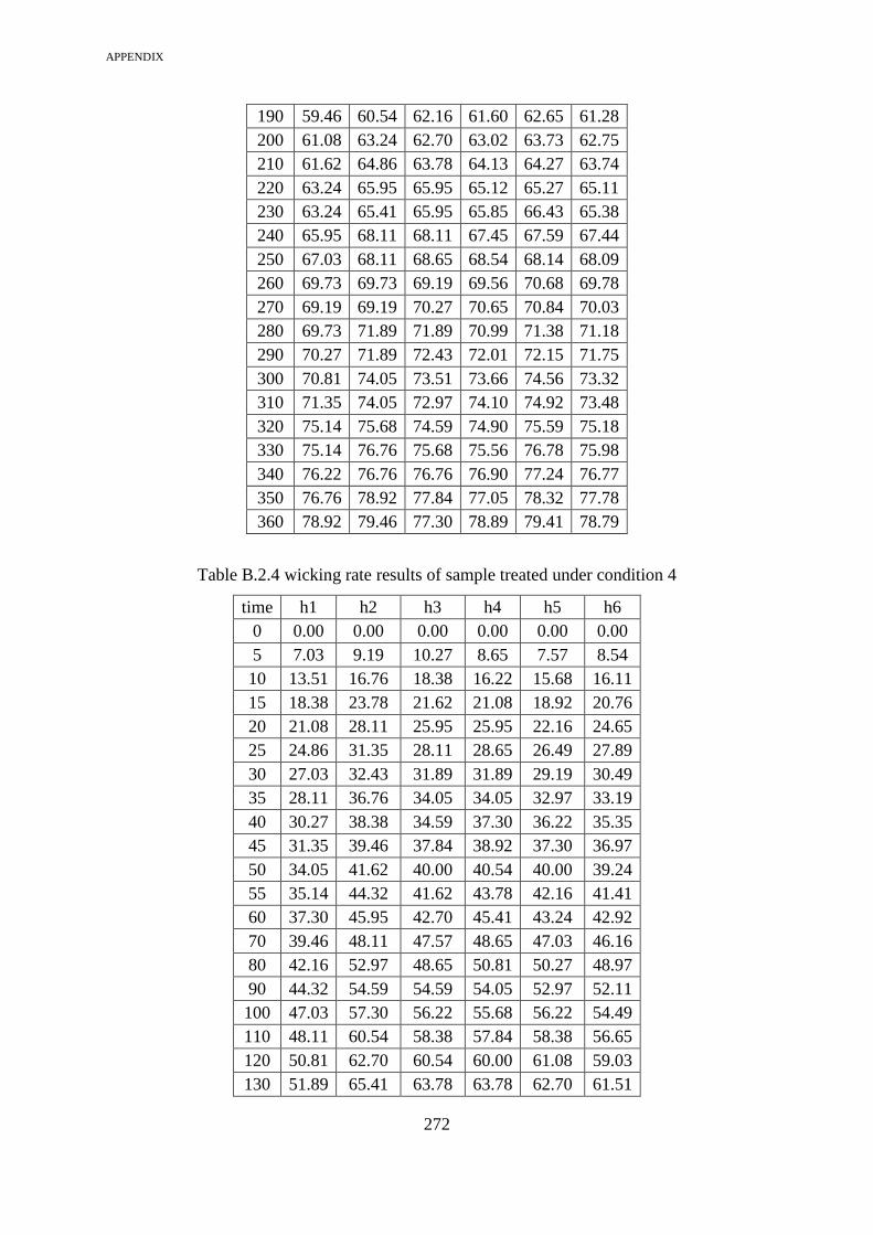
APPENDIX
272
190 59.46 60.54 62.16 61.60 62.65 61.28
200 61.08 63.24 62.70 63.02 63.73 62.75
210 61.62 64.86 63.78 64.13 64.27 63.74
220 63.24 65.95 65.95 65.12 65.27 65.11
230 63.24 65.41 65.95 65.85 66.43 65.38
240 65.95 68.11 68.11 67.45 67.59 67.44
250 67.03 68.11 68.65 68.54 68.14 68.09
260 69.73 69.73 69.19 69.56 70.68 69.78
270 69.19 69.19 70.27 70.65 70.84 70.03
280 69.73 71.89 71.89 70.99 71.38 71.18
290 70.27 71.89 72.43 72.01 72.15 71.75
300 70.81 74.05 73.51 73.66 74.56 73.32
310 71.35 74.05 72.97 74.10 74.92 73.48
320 75.14 75.68 74.59 74.90 75.59 75.18
330 75.14 76.76 75.68 75.56 76.78 75.98
340 76.22 76.76 76.76 76.90 77.24 76.77
350 76.76 78.92 77.84 77.05 78.32 77.78
360 78.92 79.46 77.30 78.89 79.41 78.79
Table B.2.4 wicking rate results of sample treated under condition 4
time h1 h2 h3 h4 h5 h6
0 0.00 0.00 0.00 0.00 0.00 0.00
5 7.03 9.19 10.27 8.65 7.57 8.54
10 13.51 16.76 18.38 16.22 15.68 16.11
15 18.38 23.78 21.62 21.08 18.92 20.76
20 21.08 28.11 25.95 25.95 22.16 24.65
25 24.86 31.35 28.11 28.65 26.49 27.89
30 27.03 32.43 31.89 31.89 29.19 30.49
35 28.11 36.76 34.05 34.05 32.97 33.19
40 30.27 38.38 34.59 37.30 36.22 35.35
45 31.35 39.46 37.84 38.92 37.30 36.97
50 34.05 41.62 40.00 40.54 40.00 39.24
55 35.14 44.32 41.62 43.78 42.16 41.41
60 37.30 45.95 42.70 45.41 43.24 42.92
70 39.46 48.11 47.57 48.65 47.03 46.16
80 42.16 52.97 48.65 50.81 50.27 48.97
90 44.32 54.59 54.59 54.05 52.97 52.11
100 47.03 57.30 56.22 55.68 56.22 54.49
110 48.11 60.54 58.38 57.84 58.38 56.65
120 50.81 62.70 60.54 60.00 61.08 59.03
130 51.89 65.41 63.78 63.78 62.70 61.51

APPENDIX
273
140 53.51 65.41 66.49 63.78 65.41 62.92
150 55.68 70.27 65.41 65.41 68.11 64.97
160 57.84 72.43 68.65 69.19 69.73 67.57
170 58.38 75.14 72.43 71.89 72.43 70.05
180 60.00 75.68 72.43 72.43 72.43 70.59
190 61.62 80.00 72.97 75.68 72.43 72.54
200 62.70 79.46 75.68 76.76 77.30 74.38
210 63.78 82.70 77.84 78.92 77.84 76.22
220 64.32 84.32 79.46 80.00 81.08 77.84
230 67.03 86.49 82.16 81.08 81.62 79.68
240 66.49 86.49 84.32 82.16 83.24 80.54
250 67.57 89.19 85.41 82.70 85.95 82.16
260 69.73 89.73 87.03 84.86 86.49 83.57
270 72.97 91.89 88.11 87.57 87.57 85.62
280 73.51 91.89 88.65 89.19 89.73 86.59
290 75.14 93.51 91.89 89.73 90.27 88.11
300 75.14 95.68 91.35 92.43 92.43 89.41
310 76.76 96.76 95.14 91.89 94.05 90.92
320 77.84 99.46 95.14 91.89 94.59 91.78
330 78.38 99.46 96.22 93.51 95.68 92.65
340 78.92 103.24 98.38 96.22 97.30 94.81
350 80.54 103.78 98.38 97.30 99.46 95.89
360 84.54 104.86 100.00 96.22 100.54 97.23
Table B.2.5 wicking rate results of sample treated under condition 5
time h1 h2 h3 h4 h5 h6
0 0.00 0.00 0.00 0.00 0.00 0.00
5 7.03 11.35 7.57 12.43 6.49 8.97
10 16.76 20.00 16.76 19.46 17.30 18.05
15 23.24 24.86 23.78 28.11 22.70 24.54
20 27.57 29.19 27.57 30.81 25.95 28.22
25 29.73 33.51 30.81 33.51 29.73 31.46
30 35.14 36.22 34.59 37.84 32.43 35.24
35 36.76 38.38 36.76 39.46 36.76 37.62
40 40.00 41.08 40.54 42.16 39.46 40.65
45 43.24 44.32 43.24 44.32 41.08 43.24
50 44.86 45.95 44.32 46.49 42.70 44.86
55 45.41 49.19 47.57 47.57 45.95 47.14
60 46.49 50.27 49.73 49.73 47.03 48.65
70 51.89 54.05 51.89 52.97 50.27 52.22

APPENDIX
274
80 54.59 57.30 55.14 56.76 54.59 55.68
90 60.00 60.00 57.30 59.46 57.84 58.92
100 63.24 62.16 61.08 62.70 61.62 62.16
110 64.86 65.41 64.32 65.41 62.70 64.54
120 67.03 69.19 66.49 67.57 66.49 67.35
130 68.65 72.43 68.11 70.27 67.57 69.41
140 71.35 73.51 71.35 72.43 70.27 71.78
150 72.97 75.14 72.97 73.51 72.97 73.51
160 74.59 77.30 75.68 75.68 73.51 75.35
170 77.30 80.00 77.84 78.38 75.68 77.84
180 80.00 80.54 79.46 78.38 77.84 79.24
190 80.54 83.78 81.62 79.46 80.54 81.19
200 82.70 84.32 83.24 83.24 80.00 82.70
210 86.49 86.49 85.41 85.41 82.70 85.30
220 87.03 88.65 87.03 85.41 84.86 86.59
230 89.19 89.73 89.19 88.11 87.03 88.65
240 90.27 92.97 89.73 89.73 89.19 90.38
250 92.43 93.51 92.43 89.73 90.81 91.78
260 93.51 95.14 93.51 92.43 91.35 93.19
270 95.14 97.30 95.14 92.97 94.05 94.92
280 97.84 96.76 97.30 94.59 94.59 96.22
290 97.30 98.38 97.84 97.30 96.22 97.41
300 99.46 99.46 99.46 98.38 97.84 98.92
310 101.62 101.62 100.54 98.92 98.92 100.32
320 103.24 101.62 102.16 101.08 100.54 101.73
330 102.70 104.86 104.86 101.08 102.16 103.14
340 105.41 105.95 104.32 104.86 103.78 104.86
350 107.57 107.57 106.49 105.95 104.86 106.49
360 107.03 109.19 108.65 107.03 105.95 107.57
Table B.2.6 wicking rate results of sample treated under condition 6
time h1 h2 h3 h4 h5 h6
0 0.00 0.00 0.00 0.00 0.00 0.00
5 10.27 10.81 10.81 9.65 9.73 10.25
10 19.46 21.08 19.46 18.22 16.22 18.89
15 23.24 25.41 24.86 22.54 21.08 23.43
20 27.57 31.89 29.19 24.16 24.78 27.52
25 32.43 35.14 31.89 28.41 27.57 31.09
30 34.59 37.30 36.76 33.65 31.19 34.70
35 35.00 41.62 37.30 34.81 35.43 37.29
40 39.46 44.32 40.00 38.59 38.14 40.10
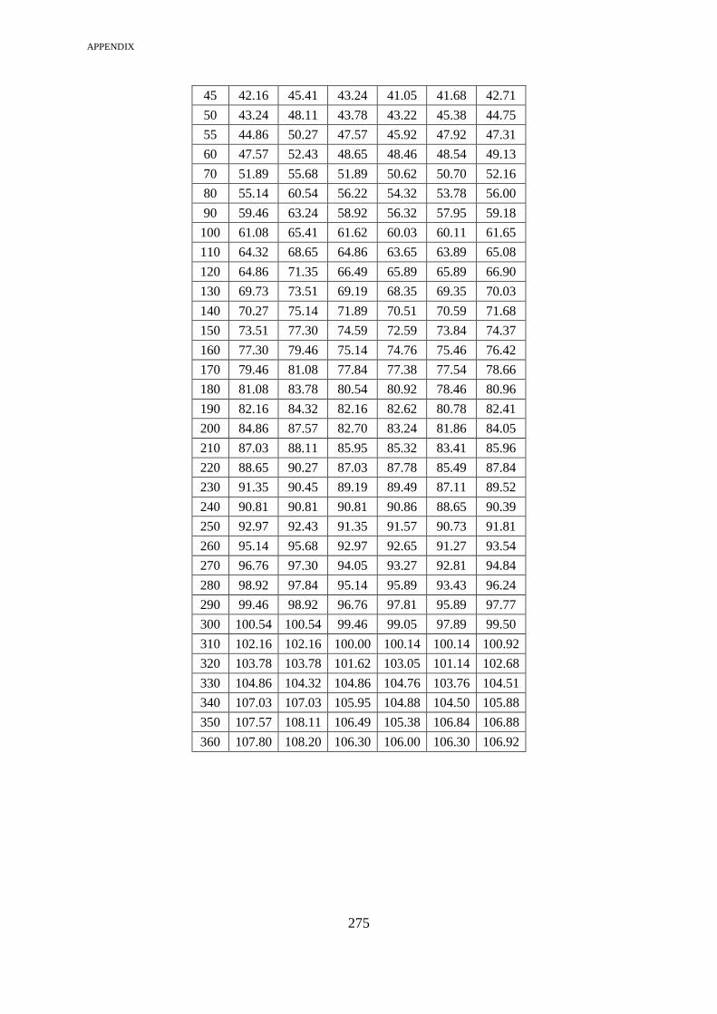
APPENDIX
275
45 42.16 45.41 43.24 41.05 41.68 42.71
50 43.24 48.11 43.78 43.22 45.38 44.75
55 44.86 50.27 47.57 45.92 47.92 47.31
60 47.57 52.43 48.65 48.46 48.54 49.13
70 51.89 55.68 51.89 50.62 50.70 52.16
80 55.14 60.54 56.22 54.32 53.78 56.00
90 59.46 63.24 58.92 56.32 57.95 59.18
100 61.08 65.41 61.62 60.03 60.11 61.65
110 64.32 68.65 64.86 63.65 63.89 65.08
120 64.86 71.35 66.49 65.89 65.89 66.90
130 69.73 73.51 69.19 68.35 69.35 70.03
140 70.27 75.14 71.89 70.51 70.59 71.68
150 73.51 77.30 74.59 72.59 73.84 74.37
160 77.30 79.46 75.14 74.76 75.46 76.42
170 79.46 81.08 77.84 77.38 77.54 78.66
180 81.08 83.78 80.54 80.92 78.46 80.96
190 82.16 84.32 82.16 82.62 80.78 82.41
200 84.86 87.57 82.70 83.24 81.86 84.05
210 87.03 88.11 85.95 85.32 83.41 85.96
220 88.65 90.27 87.03 87.78 85.49 87.84
230 91.35 90.45 89.19 89.49 87.11 89.52
240 90.81 90.81 90.81 90.86 88.65 90.39
250 92.97 92.43 91.35 91.57 90.73 91.81
260 95.14 95.68 92.97 92.65 91.27 93.54
270 96.76 97.30 94.05 93.27 92.81 94.84
280 98.92 97.84 95.14 95.89 93.43 96.24
290 99.46 98.92 96.76 97.81 95.89 97.77
300 100.54 100.54 99.46 99.05 97.89 99.50
310 102.16 102.16 100.00 100.14 100.14 100.92
320 103.78 103.78 101.62 103.05 101.14 102.68
330 104.86 104.32 104.86 104.76 103.76 104.51
340 107.03 107.03 105.95 104.88 104.50 105.88
350 107.57 108.11 106.49 105.38 106.84 106.88
360 107.80 108.20 106.30 106.00 106.30 106.92

APPENDIX
276
Table B.2.7 wicking rate results of sample treated under condition 7
time h1 h2 h3 h4 h5 h6
0 0.00 0.00 0.00 0.00 0.00 0.00
5 5.95 10.81 10.27 5.95 9.38 8.47
10 12.43 16.22 14.05 14.89 15.32 14.58
15 15.14 18.92 18.38 20.00 16.03 17.69
20 18.38 20.54 20.54 21.70 21.46 20.52
25 21.62 23.24 22.16 24.95 23.43 23.08
30 24.32 24.86 24.86 25.57 25.59 25.04
35 25.95 27.03 27.03 28.65 27.49 27.23
40 27.03 29.73 28.65 29.27 28.36 28.61
45 27.57 31.35 28.65 31.51 30.46 29.91
50 30.27 32.43 30.81 33.05 31.56 31.62
55 31.35 34.05 32.43 34.68 33.17 33.14
60 33.51 34.59 34.59 35.68 33.86 34.45
70 36.22 38.92 36.22 38.92 38.05 37.66
80 37.84 39.46 38.38 40.08 38.85 38.92
90 39.46 43.24 40.00 42.86 40.23 41.16
100 40.00 44.32 40.54 43.41 43.16 42.29
110 43.24 45.41 43.24 45.11 45.37 44.47
120 46.49 47.57 45.41 47.65 46.90 46.80
130 48.65 48.65 48.11 49.89 47.62 48.58
140 47.57 50.81 49.73 50.89 48.89 49.58
150 50.27 52.97 50.27 52.68 51.57 51.55
160 50.81 52.97 52.43 53.76 52.16 52.43
170 56.22 56.76 54.05 55.84 55.46 55.67
180 57.30 56.22 55.14 58.55 57.11 56.86
190 58.38 57.84 55.14 59.70 58.56 57.92
200 59.46 58.92 58.38 60.32 59.06 59.23
210 62.16 60.54 60.00 62.09 63.11 61.58
220 63.78 62.70 61.62 62.49 63.59 62.84
230 64.32 64.32 61.08 63.57 65.45 63.75
240 67.03 64.86 62.70 66.65 66.57 65.56
250 66.49 65.95 63.24 67.19 66.56 65.88
260 69.73 68.11 64.32 69.35 68.89 68.08
270 70.81 69.19 66.49 70.97 70.11 69.51
280 70.81 69.73 65.95 71.59 70.90 69.80
290 72.43 72.43 67.03 72.68 73.03 71.52
300 74.05 70.81 69.73 72.84 73.90 72.27
310 75.68 74.05 69.73 74.84 74.56 73.77
320 76.22 74.59 69.19 75.90 76.25 74.43
330 80.00 75.68 70.81 80.00 78.56 77.01

APPENDIX
277
340 81.08 76.76 71.89 80.08 80.12 77.99
350 80.54 76.76 72.43 81.16 78.65 77.91
360 82.16 77.84 74.05 81.78 81.55 79.48
Table B.2.8 wicking rate results of sample treated under condition 8
time h1 h2 h3 h4 h5 h6
0 0.00 0.00 0.00 0.00 0.00 0.00
5 10.27 9.73 10.81 10.05 8.56 9.89
10 17.84 15.30 17.30 16.56 15.86 16.57
15 25.41 20.54 23.78 22.46 21.56 22.75
20 27.57 24.86 27.57 25.67 25.56 26.25
25 30.27 25.95 32.97 29.57 28.56 29.46
30 32.97 29.19 34.05 31.56 31.56 31.87
35 35.14 30.81 36.76 33.56 33.56 33.96
40 37.30 33.51 37.30 35.57 35.63 35.86
45 39.46 36.76 40.00 39.85 38.57 38.93
50 42.70 36.22 42.70 41.57 40.56 40.75
55 43.78 37.84 43.24 42.86 42.56 42.06
60 44.86 38.92 45.41 44.13 44.56 43.58
70 47.03 43.24 49.19 46.22 46.56 46.45
80 53.51 46.49 51.35 49.62 50.56 50.31
90 56.22 50.81 56.76 52.82 51.57 53.63
100 54.59 52.81 59.46 54.22 55.45 55.31
110 60.54 54.05 60.54 58.90 58.56 58.52
120 61.08 57.38 63.24 61.11 60.56 60.68
130 65.41 60.00 65.95 62.46 63.56 63.47
140 64.86 62.70 68.11 63.56 64.89 64.83
150 69.19 64.86 70.27 65.56 68.45 67.67
160 73.51 65.95 72.43 68.50 71.55 70.39
170 74.59 66.65 74.05 70.46 72.57 71.66
180 75.46 68.11 76.76 71.85 75.35 73.50
190 76.84 70.81 76.76 73.78 76.95 75.03
200 77.54 72.43 78.00 74.89 78.46 76.26
210 78.08 73.68 79.16 75.56 79.56 77.21
220 79.16 75.00 80.32 78.07 81.51 78.81
230 80.24 76.92 81.95 79.11 82.56 80.16
240 80.49 77.00 82.03 80.89 82.86 80.65
250 81.49 78.32 83.57 83.57 83.18 82.02
260 82.01 78.41 84.27 84.45 83.58 82.54
270 82.19 79.05 85.81 85.45 83.61 83.22
280 84.27 79.49 86.43 87.23 84.13 84.31

APPENDIX
278
290 86.14 81.57 86.14 87.58 84.56 85.19
300 87.97 82.81 87.22 89.57 85.58 86.63
310 88.05 83.43 89.38 90.77 86.12 87.55
320 90.14 85.97 91.01 91.87 88.11 89.42
330 91.57 87.05 93.58 92.57 90.51 91.05
340 93.46 88.22 94.00 93.46 91.76 92.18
350 94.16 89.59 95.06 95.52 92.87 93.44
360 95.16 91.84 96.16 96.71 94.99 94.97
Table B.2.9 wicking rate results of sample treated under condition 9
time h1 h2 h3 h4 h5 h6
0 0.00 0.00 0.00 0.00 0.00 0.00
5 13.51 15.68 12.43 11.89 14.58 13.62
10 18.92 20.54 19.46 17.84 19.52 19.26
15 21.08 26.49 23.78 22.16 24.21 23.54
20 26.49 29.73 27.57 26.49 28.23 27.70
25 29.19 32.97 29.19 30.27 30.56 30.44
30 31.89 35.14 32.43 32.43 33.66 33.11
35 35.68 38.92 33.51 32.43 36.15 35.34
40 37.30 39.46 36.76 37.84 38.64 38.00
45 38.92 41.62 36.76 38.38 40.57 39.25
50 38.92 42.16 40.00 42.16 41.56 40.96
55 43.24 45.41 41.08 43.78 43.72 43.45
60 46.24 45.41 44.32 45.41 44.68 45.21
70 48.11 51.35 46.49 49.19 48.65 48.76
80 49.73 53.51 48.65 51.89 51.22 51.00
90 52.43 56.76 50.27 55.14 53.45 53.61
100 56.76 56.76 55.14 54.59 55.65 55.78
110 56.76 59.46 56.22 58.38 57.58 57.68
120 60.54 63.24 59.46 60.00 60.55 60.76
130 62.70 64.32 61.08 62.70 62.33 62.63
140 64.86 68.65 62.70 68.11 65.69 66.00
150 65.95 67.57 64.86 69.19 67.11 66.94
160 69.73 72.43 67.57 70.35 70.15 70.05
170 71.89 73.51 67.57 72.97 71.56 71.50
180 72.97 75.14 68.89 72.43 72.46 72.38
190 74.59 77.30 69.43 77.84 74.58 74.75
200 74.59 77.92 69.51 77.84 74.66 74.91
210 75.84 78.08 71.05 78.22 75.66 75.77
220 76.46 78.70 72.59 78.76 76.21 76.55
230 79.97 79.16 73.68 78.77 76.89 77.69

APPENDIX
279
240 77.70 79.49 74.84 79.54 77.57 77.83
250 77.78 81.03 75.00 79.83 78.07 78.34
260 78.86 82.53 76.62 81.24 78.56 79.56
270 78.95 84.11 76.70 81.70 79.12 80.12
280 79.49 85.89 77.24 82.65 81.52 81.36
290 80.49 86.81 78.09 83.65 82.62 82.33
300 81.65 86.89 79.95 84.27 83.11 83.17
310 83.43 87.97 80.57 84.89 84.22 84.22
320 86.81 87.59 80.73 85.51 86.56 85.44
330 87.43 88.22 82.65 87.76 87.66 86.74
340 86.97 89.92 83.81 89.84 88.22 87.75
350 88.05 90.00 86.51 90.46 89.12 88.83
360 89.22 91.92 87.97 91.00 89.41 89.90
Table B.2.10 wicking rate results of sample treated under condition 10
time h1 h2 h3 h4 h5 h6
0 0.00 0.00 0.00 0.00 0.00 0.00
5 10.81 10.81 8.11 7.57 9.19 9.30
10 20.00 19.46 19.46 18.51 17.30 18.95
15 24.86 24.86 23.24 21.84 21.08 23.18
20 29.19 30.27 28.11 24.54 24.32 27.29
25 31.35 32.97 32.43 27.16 28.11 30.41
30 34.59 34.59 35.68 29.41 30.81 33.02
35 38.92 38.92 37.84 31.49 31.35 35.70
40 41.62 41.08 40.00 33.65 32.97 37.86
45 42.70 43.24 43.24 35.27 34.59 39.81
50 44.86 45.41 44.32 37.81 37.30 41.94
55 47.03 46.49 47.57 38.89 36.76 43.35
60 48.65 49.73 49.73 40.51 40.00 45.72
70 52.43 50.81 51.89 45.22 43.24 48.72
80 56.22 56.22 56.22 47.92 44.86 52.29
90 58.92 60.54 58.38 48.00 45.95 54.36
100 61.08 62.16 61.62 50.00 49.73 56.92
110 64.86 64.86 62.70 55.24 53.51 60.24
120 66.49 66.49 67.03 56.78 54.59 62.28
130 69.19 69.19 68.11 58.86 57.30 64.53
140 72.43 72.43 70.81 61.99 58.92 67.32
150 74.59 74.59 72.97 62.95 61.08 69.24
160 76.22 75.68 75.68 63.35 60.54 70.29
170 78.38 77.30 76.76 65.89 63.24 72.31

APPENDIX
280
180 81.08 82.16 80.54 67.89 66.49 75.63
190 82.16 81.08 81.62 69.05 67.57 76.30
200 84.86 83.78 83.78 70.59 69.73 78.55
210 85.41 85.41 85.95 72.68 71.35 80.16
220 85.41 88.65 87.03 75.76 71.89 81.75
230 87.57 87.57 88.11 78.92 75.14 83.46
240 91.35 91.35 90.27 80.84 77.59 86.28
250 92.43 91.35 92.97 81.00 79.76 87.50
260 94.59 93.51 92.97 83.46 81.38 89.18
270 95.14 94.05 95.68 85.08 84.30 90.85
280 98.92 97.30 96.22 87.70 86.62 93.35
290 99.46 98.92 97.84 90.24 87.86 94.86
300 98.92 100.00 97.84 93.78 89.32 95.97
310 100.54 101.08 101.62 95.86 90.11 97.84
320 101.62 102.70 102.70 98.03 91.19 99.25
330 102.70 103.24 103.24 99.03 92.65 100.17
340 105.41 105.95 103.78 102.03 93.81 102.19
350 105.41 106.49 106.49 104.27 94.19 103.37
360 108.65 109.19 107.03 106.88 96.27 105.60
Table B.2.11 wicking rate results of sample treated under condition 11
time h1 h2 h3 h4 h5 h6
0 0.00 0.00 0.00 0.00 0.00 0.00
5 10.81 9.73 10.81 10.27 10.27 10.38
10 20.00 19.46 18.38 19.46 20.54 19.57
15 25.95 24.86 24.32 24.86 25.41 25.08
20 29.73 28.11 28.11 28.11 30.81 28.97
25 33.51 30.81 30.81 31.35 32.43 31.78
30 34.59 34.05 33.51 34.59 36.76 34.70
35 37.30 34.59 37.84 36.76 41.08 37.51
40 40.54 37.84 38.38 40.54 43.24 40.11
45 42.70 39.46 42.16 42.16 46.49 42.59
50 45.95 44.32 44.86 44.32 49.19 45.73
55 47.03 45.95 45.41 47.03 51.35 47.35
60 48.65 47.03 45.41 49.19 52.97 48.65
70 52.97 50.27 48.65 52.43 57.30 52.32
80 55.14 54.05 51.89 55.68 60.54 55.46
90 58.38 56.22 55.14 54.59 63.78 57.62
100 61.62 60.54 57.30 61.62 65.41 61.30

APPENDIX
281
110 63.78 62.70 60.54 63.24 69.19 63.89
120 66.49 62.16 62.70 64.32 71.89 65.51
130 69.19 64.86 64.32 66.49 75.14 68.00
140 71.35 69.19 66.49 70.81 77.30 71.03
150 72.43 72.43 69.19 72.43 79.46 73.19
160 73.51 72.97 70.27 72.97 79.46 73.84
170 76.76 76.76 72.43 75.68 80.54 76.43
180 77.84 78.38 74.05 79.46 82.70 78.49
190 81.08 80.54 75.68 81.62 86.49 81.08
200 81.62 80.00 78.38 82.16 88.65 82.16
210 83.24 84.86 77.30 81.62 90.81 83.57
220 84.86 84.86 82.16 85.41 91.89 85.84
230 88.11 88.11 81.62 87.03 90.81 87.14
240 89.19 89.19 83.24 87.57 90.81 88.00
250 90.27 89.73 85.41 88.65 95.14 89.84
260 90.81 91.35 86.49 91.89 98.38 91.78
270 94.05 91.89 88.11 94.05 96.76 92.97
280 94.59 94.05 88.11 94.05 98.92 93.95
290 96.22 96.22 90.81 92.97 98.38 94.92
300 95.14 97.84 91.35 97.30 100.00 96.32
310 98.92 98.38 93.51 98.92 99.46 97.84
320 99.46 98.92 94.05 97.30 101.08 98.16
330 102.16 100.54 96.22 101.62 105.95 101.30
340 103.24 101.62 96.76 101.62 105.95 101.84
350 104.32 102.70 99.46 102.70 105.95 103.03
360 104.86 104.86 100.54 105.41 107.03 104.54
Table B.2.12 wicking rate results of sample treated under condition 12
time h1 h2 h3 h4 h5 h6
0 0.00 0.00 0.00 0.00 0.00 0.00
5 4.86 7.03 5.95 10.81 12.43 8.22
10 14.59 16.22 16.22 18.38 21.08 17.30
15 19.46 21.62 21.08 23.24 28.65 22.81
20 23.78 24.86 26.49 27.03 32.97 27.03
25 26.49 28.11 27.57 29.73 36.22 29.62
30 29.73 31.89 30.27 32.43 40.00 32.86
35 31.35 32.97 33.51 36.22 41.08 35.03
40 34.05 34.59 37.30 37.30 45.95 37.84
45 35.14 38.38 38.92 40.00 46.49 39.78
50 37.84 40.54 42.70 42.16 49.73 42.59
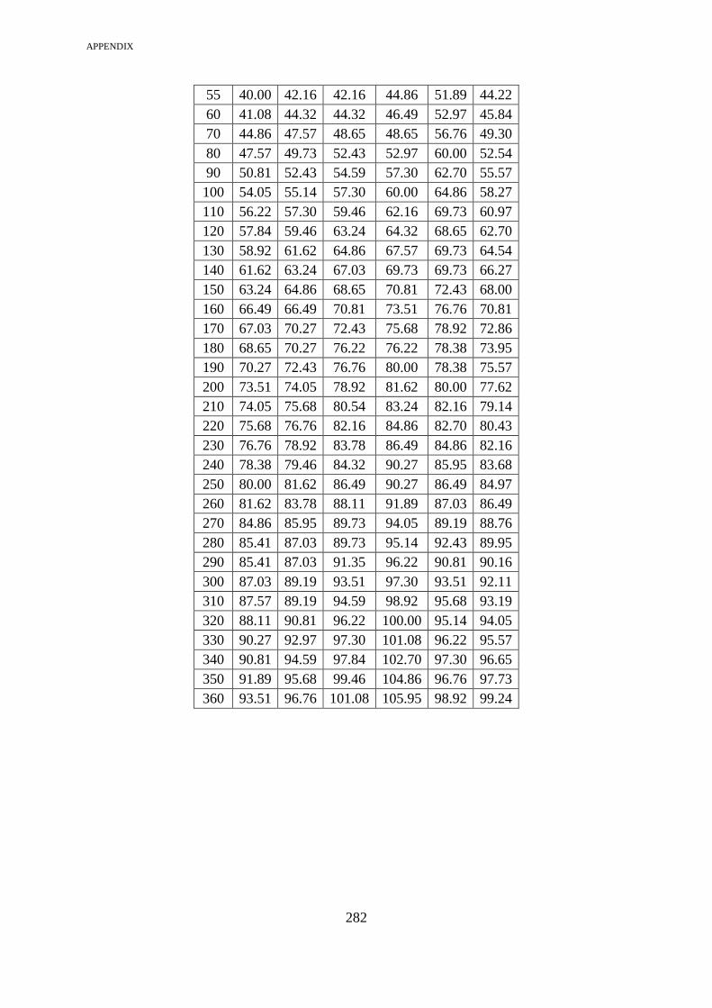
APPENDIX
282
55 40.00 42.16 42.16 44.86 51.89 44.22
60 41.08 44.32 44.32 46.49 52.97 45.84
70 44.86 47.57 48.65 48.65 56.76 49.30
80 47.57 49.73 52.43 52.97 60.00 52.54
90 50.81 52.43 54.59 57.30 62.70 55.57
100 54.05 55.14 57.30 60.00 64.86 58.27
110 56.22 57.30 59.46 62.16 69.73 60.97
120 57.84 59.46 63.24 64.32 68.65 62.70
130 58.92 61.62 64.86 67.57 69.73 64.54
140 61.62 63.24 67.03 69.73 69.73 66.27
150 63.24 64.86 68.65 70.81 72.43 68.00
160 66.49 66.49 70.81 73.51 76.76 70.81
170 67.03 70.27 72.43 75.68 78.92 72.86
180 68.65 70.27 76.22 76.22 78.38 73.95
190 70.27 72.43 76.76 80.00 78.38 75.57
200 73.51 74.05 78.92 81.62 80.00 77.62
210 74.05 75.68 80.54 83.24 82.16 79.14
220 75.68 76.76 82.16 84.86 82.70 80.43
230 76.76 78.92 83.78 86.49 84.86 82.16
240 78.38 79.46 84.32 90.27 85.95 83.68
250 80.00 81.62 86.49 90.27 86.49 84.97
260 81.62 83.78 88.11 91.89 87.03 86.49
270 84.86 85.95 89.73 94.05 89.19 88.76
280 85.41 87.03 89.73 95.14 92.43 89.95
290 85.41 87.03 91.35 96.22 90.81 90.16
300 87.03 89.19 93.51 97.30 93.51 92.11
310 87.57 89.19 94.59 98.92 95.68 93.19
320 88.11 90.81 96.22 100.00 95.14 94.05
330 90.27 92.97 97.30 101.08 96.22 95.57
340 90.81 94.59 97.84 102.70 97.30 96.65
350 91.89 95.68 99.46 104.86 96.76 97.73
360 93.51 96.76 101.08 105.95 98.92 99.24