The (In)efficiency of Share-Tenancy Revisited: Evidence

from Pakistan

Hanan G. Jacoby∗ Ghazala Mansuri∗

January 2004(very preliminary; please do not cite)

Abstract

Sharecropping has long fascinated economists, and perhaps no question has

drawn more attention than that of the efficiency of this contractual arrangement.With a couple of notable exceptions, past studies find small or insignificant productiv-

ity differentials between sharecropped and owner-cultivated land. This paper provides

more conclusive evidence using a large, nationwide, micro-data set from rural Pak-

istan. Our estimates show that the average yield differential between share-tenanted

and owner-cultivated plots is highly unlikely to exceed 8 percent. An analysis of

tenant labor allocation corroborates this conclusion.To understand why sharecropping does not lead to substantial productivity losses

on average, we use unique data on monitoring frequency collected directly from ten-

ants. We find that "unsupervised" tenants are significantly less productive than

their "supervised" counterparts. We show that the coexistence of these two types of

tenants is consistent with an agency model in which landlords have different costs of

supervision. To assess the model, we investigate whether a landlord’s decision about

the form of incentive contract and degree of supervision is driven, in part, by variationin supervision costs.

∗Development Research Group, The World Bank. Contact Information: Jacoby: e-mail: hja-coby@worldbank.org; Mansuri: e-mail: gmansuri@worldbank.org.

1 Introduction

Sharecropping has long fascinated economists, and perhaps no question has drawn

more attention than that of the efficiency of this contractual arrangement. Writers in

the "Chicago" tradition (e.g., Johnson, 1950; Cheung, 1968; Reid, 1977) argued that the

incentive problem inherent in share-tenancy is largely obviated by the landlord’s supervi-

sion. With the advent of agency theory, in which sharecropping was a leading example

(Stiglitz, 1974), the notion that the tenant’s effort could be effectively monitored, and

hence contracted upon, began to be regarded with skepticism.1 In a landmark study,

Shaban (1987) vindicated the moral hazard paradigm by finding lower labor intensity and

yields on sharecropped land as compared with owner-cultivated land. Sharecropping,

at least in the six South Indian villages investigated by Shaban, did lead to substantial

productivity losses. Broader evidence from a tenancy reform in West Bengal (Banerjee,

et al., 2002) only reinforces this view, showing that even a modest reallocation of property

rights in favor of share-tenants can have dramatic productivity effects.

Notwithstanding these two prominent studies from India, the idea that share-tenancy

entails serious inefficiency, in general, remains controversial. Much, if not most, other

evidence points to small or insignificant productivity differentials, though clearly some of

these findings can be attributed to small sample sizes or to other methodological short-

comings (Otsuka, et al., 1992; Binswanger, et al., 1995).2 This paper aims to provide

more conclusive evidence using a large, nationwide, micro-data set from rural Pakistan,

a country with an agriculture similar to that of India, but where tenancy is even more

common.

The empirical work in this paper is divided into two parts. In the first part, presented

in Section 3, we estimate the average yield differential between share-tenanted and owner-

cultivated plots. Based on these estimates, we are able to state with a high degree of

confidence that this differential does not exceed 8 percent and is most likely smaller. Thus,

we can easily rule out yield differentials of, respectively, 16 percent (Shaban) and more

than 50 percent (Banerjee, et al.) in the Pakistani context.3 Our analysis of tenant labor

1Indeed, Stiglitz provides a vivid and detailed discussion of the "quality" of the tenant’s labor inagricultural production and how it is inherently difficult to contractually specify and enforce.

2The well-known study of Laffont and Mattousi (1995), for example, is based on fewer than 200 plotsfrom a single Tunisian village. Possibly as a consequence, none of the differences in productivity betweenshare-tenants and owner/renters that they estimate appear to be statistically significant. Moreover,their point estimates indicate that, at the sample mean of tenancy contract duration, productivity onsharecropped land is actually higher than on owner-cultivated land!

3The impressive productivity gains on sharecropped land found by Banerjee et al. are all the more

1

allocation, similar to that of Shaban (except, in our case, broken down by agricultural

task), corroborates this conclusion.

The second part of the empirical work asks why sharecropping does not lead to sub-

stantial productivity losses in Pakistan, at least on average. In Section 4, we reconsider

the question of landlord supervision. Using unique information on monitoring frequency

collected directly from tenants, we find that "unsupervised" tenants are significantly less

productive than their "supervised" counterparts. We show that the coexistence of these

two types of tenants is consistent with an agency model in which landlords have different

costs of supervision. To assess the model, we go on to investigate whether a landlord’s

decision about the form of incentive contract and degree of supervision is driven, in part,

by variation in supervision costs.

Before turning to these results, however, we set out the context for our study in the

next section along with the framework for the empirical analysis. Section 5 concludes the

paper.

2 Analytical Framework

2.1 Data

Our empirical analysis draws mainly upon a new nationally representative rural house-

hold survey. The Pakistan Rural Household Survey (PRHS), which was completed in late

2001, collected data from about 2,800 households sampled across 17 districts and 150

villages. Roughly 60 percent of the households surveyed were farm households and a con-

siderable fraction of these operated multiple plots. The survey was designed to provide

detailed information at the plot level on land characteristics (soil type, irrigation, and so

forth), land tenancy contracts, and production activities. These data were collected for

the two major agricultural seasons, kharif (May-November) and rabi (November-May).

The principal cash crops, cotton, rice, and sugarcane, are grown in kharif, while the main

food crop, wheat, is grown in rabi.

The 2001 PRHS was modeled upon and surveyed some of the same households as

round 14 of the IFPRI panel survey. This smaller survey, fielded in 1993, was carried

remarkable considering that the tenancy reform in West Bengal fell far short of providing share-tenantsthe same incentives as owner-cultivators. Were moral hazard in current production effort the only source ofinefficiency, their estimates could thus be viewed as a lower bound on the effect of converting sharecroppedland into owner-cultivated land. However, as they point out, the tenancy reform may also have raisedland productivity by improving investment incentives for share-tenants.

2

out in only four districts and 5? villages. Because much of the plot-level agricultural

production and tenancy data are comparable across the two surveys, part of our empirical

work pools the 2001 and 1993 surveys to improve the precision of our estimates.

2.2 Context

Pakistan has a very unequal distribution of landownership. Consequently, the fraction of

tenanted land is high (about a third), and about two-thirds of it is under sharecropping.

Description of sharecropping....regional variation in contract terms, etc.

2.3 Moral hazard and yields

To clarify the empirical issues, we consider a simple tenancy model with a constant

returns to scale technology. This avoids having to model the choice of plot size, which we

set to unity. Gross output, or yield, is given by the production function y = f(e, x) + ε,

which depends on unmonitorable tenant effort e and a purchased input (e.g., fertilizer) x,

as well as a random shock ε. Net productivity is given by π = y − px, where p is theprice of the purchased input normalized by the price of output. The tenant’s disutility of

total effort is given by the convex function v(e). The share-contract specifies an output

share β and possibly also a fixed component α, which may be negative. The cost of the

purchased input is shared between landlord and tenant at the same rate as output.

A risk neutral tenant chooses e and x such that βfe = v and fx = p,4 from which we

may write y = g(β, p)+ε. Given that any tenancy contract must be incentive-compatible,

moral hazard delivers the unambiguous prediction de∗dβ > 0, where stars denote the tenant’s

optimal choice. The marginal effect of share-tenancy on yields, however, is given by

dy

dβ= fe

de∗

dβ+ fx

dx∗

dβ

which, in general, is ambiguous.5 If e and x are perfect substitutes, for example, pro-

viding the tenant better incentives does not actually increase yields at all (of course, in

this case, the landlord could dispense with the tenant altogether and use only fertilizer).

More generally, a test of the null of zero moral hazard using yield data only has power

against alternatives in which moral hazard is present and tenant effort is an input without

4Actually, precisely the same first-order conditions would hold for a risk-averse tenant in this formula-tion. Later, however, we model share-tenancy as arising from financial constraints, so we do not need torely on tenant risk aversion.

5The sufficient condition for a positive yield effect is that fxe > fefxx/fx

3

very close purchased substitutes.6 Also, the extent to which a purchased input, such as

fertilizer, is substitutable with tenant effort (i.e., dx∗

dβ = dxdede∗dβ ) is indicated by just how

much more of this input is used on tenanted plots than on owner cultivated plots.7

2.4 Empirical model and the selection problem

Our regression model for yields realized by cultivator c on plot i is

yci = γsci + θ xci + νc + ηci (1)

where sci is an indicator of whether the plot is sharecropped, β ∈ (0, 1), and xci is avector of exogenous plot characteristics. Thus, γ estimates the yield differential between

sharecropped plots on the one hand and owner-cultivated and rented plots on the other.

One component of the error, νc, captures all unobserved factors common to a given culti-

vator that determine productivity; e.g., access to credit, farming knowledge, average land

quality, and ownership of non-marketed assets more generally. Included in this term

would also be the effect of input prices, p, to the extent that these are not observed. The

error component ηci contains plot-specific unobservables, such as soil fertility, that are not

captured by xci.

In general, the decision to enter into a sharecropping contract will depend upon the

cultivator’s unobserved characteristics (i.e., E [νc | sci = 1] = 0), which leads to a selec-

tion (or endogeneity) bias in 1. All of the major theories of share-tenancy that have thus

far been proposed in the literature, however, imply that sharecroppers have lower un-

observed productivity than owner-cultivators or fixed renters, which imparts a particular

direction to the selection bias. For example, models with either ex-post or ex-ante finan-

cial constraints (Shetty, 1998; Basu, 1992; Mookherjee, 1997; Laffont and Mattoussi, 1995)

imply that wealthier cultivators would be less likely to take land on share, but wealthier

cultivators, if anything, will tend to have higher productivity on a given piece of land.

An analogous argument would apply if share-tenancy is motivated by risk aversion (e.g.,

6For this reason, it might seem more attractive to compare net rather than gross productivity. Inparticular, dπ∗

dβ = fede∗dβ is unambiguously positive. The problem, in practice, is that there are usually

several purchased inputs, each measured with considerable noise, so that net productivity tends to be lessprecisely measured than gross productivity. Moreover, estimates based on yield data are more comparableto those from previous studies.

7Note that we do not need to assume that x is contractible. Although fertilizer, for example, canbe readily purchased, it may be difficult to enforce a contract in which a tenant uses a quantity that isincompatible with his first-order conditions. The key feature that distinguishes e and x is that the costof effort is not observable to the landlord and hence cannot be shared with his tenant.

4

Stiglitz, 1974); i.e., share tenants are more risk averse, but greater risk aversion reduces

productivity by, for instance, encouraging the use of safer but less effective production

techniques. In the double-sided moral hazard model of Eswaran and Kotwal (1985), both

tenant and landlord supply a noncontractible input, which in the landlord’s case may

be farming know-how. Here, again, sharecroppers tend to come from the lower tail of

the productivity distribution. The same holds when farming ability is private informa-

tion to the tenant, as in Halligan’s (1978) screening model — less able cultivators become

sharecroppers rather than fixed renters.

If sharecroppers are indeed, on average, less productive farmers, then we expect that

estimates of γ that fail to account for this selectivity will overstate the disincentive effects

of share-tenancy. In other words, the OLS estimate of γ will tend to be negative even

if the true γ is zero. A corollary to this observation is that if the OLS estimate of γ is

in fact zero, then the selection problem is not likely to be empirically important. This

is because, under either the null of no moral hazard or under the alternative of moral

hazard, the true γ cannot plausibly be positive.

Our strategy for correcting the selectivity bias is essentially the same as that of Shaban

(1987) and Bell (1977). We use household fixed effects to purge νc, a procedure that

requires a sufficient number of owner-cum-sharecropper, households that cultivate at least

one sharecropped plot and one plot of their own (or one plot on fixed rent). Even after

taking out household fixed effects, there is no guarantee that E [ηci | sci = 1] = 0. Highlyfertile plots may be more (or less) likely to be sharecropped out than those cultivated by

their owners or given on fixed rent. Unfortunately, finding good instruments for within

household variation in sci is difficult, so we will have to rely on indirect methods to assess

this potential endogeneity problem.

3 Results: Is Sharecropped Land Less Productive?

3.1 Yields

To obtain precise estimates of productivity differentials, we focus on yield from the

five major crops: wheat, rice, cotton, sugarcane, and maize. We thus exclude the value

of outputs from fodder and a number of minor crops, which are difficult to measure

accurately. In the 1993 IFPRI sample, major crops account for 66% of cultivated area

(71% for sharecropped land), whereas in the nationally representative 2001 PRHS, 80% of

5

cultivated area is devoted to major crops (83% for sharecropped land). Yield is defined

as the value of output from these five crops (evaluated at median prices for that year)

divided by the area of the plot planted to major crops over kharif and rabi seasons. Plots

growing none of the major crops are dropped from the sample, as are cases of yield above

the 99th percentile (the presence of which inflates the standard errors). Table 1 breaks

down the number of plots available, by year. For the household fixed effects analysis of

yields, the sample consists of the 1,718 plots belonging to households with multiple plots.8

Of these, 403 belong to owner-cum-sharecropper households; these plots directly identify

the share-tenancy effect.9 The remaining 1,315 plots, belonging to pure sharecroppers or

pure owner-cultivator households, contribute to greater precision when we control for plot

characteristics.

Table 2 presents household fixed effects results for yields. The dependent variable

is scaled so that the coefficients can be interpreted as percentage deviations relative to

owner-cultivators/fixed renters. Unconditional on plot attributes, we see that yields are

about 3% lower on share-tenanted plots, a difference which is not remotely significant.

Controlling for plot characteristics (value, area, irrigation, soil, etc.; see Appendix) hardly

changes this result.10 Evidently, these important observed characteristics are not highly

correlated with the tenancy status of the plot. In light of this, it would be surprising

if the presence of unobserved plot characteristics (e.g., soil fertility) would seriously bias

our results. Adding crop composition variables (i.e., the fraction of area cultivated with

major crops devoted to a given crop) also has little effect, except to slightly improve the

precision of the sharecropping coefficient estimate. While, in theory, crop choice may

be specified in the tenancy contract, and hence endogenous, in Pakistan, share-tenants

generally have autonomy over crop choice and grow basically the same mix of crops as

owner-cultivators.11

Failure to reject the null hypothesis of equal gross productivity across tenure types is

informative only to the extent that moderate productivity differences would be detectable

8Although most households from the 1993 round are resurveyed in 2001, we do not make use of thepanel element in the estimation. Grouping together the plots of the same household in different surveyrounds results in less precise estimates as compared to treating them as separate households in each round.

9Owner-cum-sharecropper households are over-represented in the IFPRI survey by geographical acci-dent; these households tend to be concentrated in central Punjab.10Shaban (1987), by contrast, finds that the yield differential falls by more than one third, from 25% to

16%, once he controls for irrigation and other plot characteristics.11For all five of the major crops in our yield measure, there is no significant difference in the proportion

of area cultivated between share tenanted and other plots, once we control for tehsil (there are 23 tehsilsin our sample).

6

in our data. Andrews (1989) has devised a statistic, the inverse power function, that

allows one to quantify the set of alternatives against which a given test has power. Table

2 reports, next to each estimate, two points along the inverse power function. The first

point is the percentage yield differential against which our test has low power. Based on

the household fixed effects estimates, we would be equally likely as not to reject the null if

the true yield differential were around 7%; this figure demarcates the region of low power.

On the other hand, if the true yield differential were 13%, we would be 95% certain of

rejecting the null. Thus, our test has high power against yield differentials exceeding

13%.

Although 13% is a respectable number, we can do even better by imposing restrictions

in the estimation. To this end, we report analogous estimates using village, rather than

household, fixed effects. These estimates are not robust to the selection problem outlined

above, but they do control for input price variation across villages and may be more effi-

cient than household fixed effects estimates.12 As it happens, all of the village fixed effects

estimates are within a single standard error of their household fixed effects counterparts.

This finding suggests that selection into share-contracts on cultivator-specific unobserv-

ables is not particularly strong.13 Moreover, the standard error on the sharecropping

dummy coefficient falls by almost 40% as we move to the village fixed effects estimator.

As a consequence, the inverse power interval (which is proportional to this standard error)

shifts to the left. We can now be 95% certain that the yield differential is no greater than

8%, whereas our test has low power against only fairly trivial yield differentials, below 4%.

3.2 Nitrogen

As discussed above, to test for moral hazard using yield data one needs to maintain

the assumption that tenant effort has no close purchased substitutes. However, if such

substitutes exist, then they must respond to marginal incentives in the opposite direction

as tenant effort. In other words, these inputs must be used more intensively on share-

cropped plots than on owner-cultivated plots. A relatively clean test-case is provided by

chemical fertilizer, a major purchased input in Pakistan. We focus on nitrogen, which

12Note that this estimator uses all 2,807 plots in the sample, including those belonging to single-plothouseholds. In the estimation, we also allow for household random effects to deal with the correlationacross plots within multi-plot households.13Again using the inverse power function calculation, we can be 95% certain that the household fixed

effect estimate of the yield differential is within about 11 percentage points of the village fixed effect(household random effect) estimate. In other words, we would be very likely to detect moderate selectionbias if it existed in our data.

7

is more widely used than phosphate. Nitrogen has the advantage of being a very ho-

mogeneous input compared to, say, seed and even tractor services. Moreover, the costs

of fertilizer are generally, but not universally (see below), shared between landlord and

tenant at the same rate as output. Since share-tenancy, consequently, does not distort

the fertilizer margin, differences in fertilizer intensity across tenure types are driven solely

by complementarity or substitutability between fertilizer and tenant effort.

The bottom panel of Table 2 presents estimates of equation 1 with yields replaced by

the quantity of nitrogen in kg per acre. We expand the sample to include all cultivated

plots, not just those growing major crops (see Table 1). In about one quarter of the share-

tenancies, fertilizer costs are either the sole responsibility of the tenant or the tenant bears

a larger share of the cost than he receives in output. In these cases, the share-contract

may indeed distort the fertilizer margin. But when we include an indicator variable to this

effect in the fertilizer regressions, it never attains statistical significance. To maximize

precision, we omit this variable from the results reported below.

The point estimate of the sharecropping dummy coefficient for nitrogen use in Table

2 is indistinguishable from zero in every specification. Inverse power function thresholds

are, in this case, positive numbers because we are only interested in alternatives wherein

sharecroppers use nitrogen more intensively than owner-cultivators. Based on the house-

hold fixed effects standard errors, we can be confident that the nitrogen differential is no

greater than 16%. Using the village fixed effects estimates instead, this threshold drops

to just 10%. In short, there is little chance that the lack of a yield effect is due to the

substitutability of nitrogen for tenant effort. Of course, this evidence is not decisive in

itself, as there may be other purchased inputs that substitute for effort.

3.3 Labor

A more direct test for moral hazard involves comparing the cultivator’s family la-

bor input on sharecropped versus owned plots. Indeed, perhaps the most compelling

piece of evidence from Shaban’s (1987) study is that owner-cum-sharecroppers allocate

substantially less family labor to their tenanted plots than they do to their owned plots.

Naturally, the question arises as to how well reported labor hours on a plot correspond to

cultivator ’effort’ when the quality of labor is variable, but the fact remains that Shaban’s

finding has been widely viewed as indicating moral hazard in effort.

The 1993 IFPRI survey (but not the 2001 PRHS) provides information on plot-level

labor inputs, both hired and family. These data are disaggregated by type of worker

8

(adult male and female, and male and female child), but since the vast majority of farm

labor is supplied by adult men in this sample, we combine the hours of all worker types.

Unlike the ICRISAT data used by Shaban, the IFPRI survey collects farm labor data by

major task (plowing/irrigation, sowing, weeding, harvesting, and threshing). To analyze

labor use, we modify our previous procedure in one respect by taking logs of labor hours

instead of using levels, as the former gives us considerably lower standard errors.14

Table 3 shows results with alternative definitions of labor hours per acre, and with each

regression including the full set of controls (plot characteristics and crop composition).

Based on the household fixed effects estimates, we find that family labor, aggregated

across all tasks, is about 6% lower on sharecropped plots than on owner-cultivated plots.

Once again, this difference is not significant, but the standard errors are noticeably larger

than in Table 2. The village fixed effects estimate is a bit more precise, but in this

case a Hausman test rejects equality between the (household) fixed and random effects

coefficients (p-value = 0.006). Conservatively, then, our test has high power against

family labor use differentials of around 21%. Shaban (1987) estimates a family labor use

differential of exactly 21% for males (47% for females). Based on our findings, we can all

but rule out such high differentials in the case of Pakistan.

The second specification in Table 3 combines family and hired labor. Shaban’s analysis

found that hired labor use was modestly lower on sharecropped plots than on owned plots

cultivated by the same household. It is also conceivable, as discussed earlier, that hired

labor substitutes for tenant effort and is thus used more intensively on share-tenanted

land. If anything, our evidence suggests the latter scenario, as the percentage differential

in total (family + hired) labor use is closer to zero than that of family labor alone, although

the relatively high standard errors preclude firm conclusions.

Certain tasks are inherently easier to monitor than others. For example, in contrast to

other activities, much of hired harvest labor in Pakistan is paid on a piece-rate (see Jacoby

and Mansuri, 2003), which suggests that monitoring and enforcement are feasible for this

task. Probably for this very reason, the cash costs incurred for harvesting/threshing

(principally hired labor) are more frequently shared between landlord and tenant than in

the case of land preparation (plowing, sowing, and weeding). Combining time spent on

land preparation and on harvesting may obscure any moral hazard effects present in the

former but not in the latter.

To investigate this issue, we re-run the labor-use regressions excluding hours spent14Standard errors of percentage changes are calculated using the approximation formula given by van

Garderen and Shah (2002).

9

harvesting and threshing. These two activities account for almost half of all family labor

hours devoted to the average plot. Surprisingly, the family labor-use differential between

sharecropped and owner-cultivated plots does not increase when we focus solely on land

preparation tasks. To the contrary, the differential based on the household fixed effects

estimates is actually closer to zero, although the corresponding results for total labor are

practically identical.

Overall, then, the findings do not favor the implications of moral hazard in tenant

effort. What paltry evidence there is of lower family labor intensity on sharecropped land

is belied by the failure of this effect to strengthen when we concentrate on tasks that are

likely to be particularly susceptible to moral hazard.

4 Does Landlord Supervision Matter?

The results of the previous section rule out a sizeable yield shortfall on share-tenanted

land vis a vis owner-cultivated/rented land. Faced with similar, albeit less conclusive,

evidence, Otsuka, et al. (1992) surmise that supervision (and enforcement) of share-tenant

effort is generally effective. Sharecropping, they argue, is adopted only when monitoring

costs are low enough to make it worthwhile relative to fixed rental. They go on to suggest

that "significant inefficiency of share-tenancy is expected to arise only when the scope of

contract choice is institutionally restricted" (p. 2007). Where fixed rent tenancy is legally

discouraged, landlords without a comparative advantage in supervision are forced to enter

into sharecropping contracts. Thus, rather than evidence of the general inefficiency of

sharecropping, these authors view Shaban’s (1987) findings as a peculiarity arising from

India’s legal environment. Land-to-the-tiller legislation effectively penalized landlords

who entered into longer-term tenancy, which tended to be under fixed rent. Many land-

lords thus shifted into short-term share-tenancy contracts, ill-equipped with the requisite

supervision technology.

As attractive as this argument may sound, the proposition that sharecropper ineffi-

ciency declines with the degree of supervision has yet to be subjected to formal empirical

testing. In this section, we provide such a test, but, before doing so, we need to under-

stand why, in equilibrium, two otherwise identical tenants might receive different levels of

supervision. We begin, then, by setting out a model of landlord supervision that forms

the basis for our empirical work in the remainder of this section. The model has impli-

10

cations for the relationship between yields and the level of supervision as well as for how

supervision costs determine the form of the tenancy contract.

4.1 A tenancy model with supervision

Returning to the set-up of subsection 2.3, suppose that the tenant faces an ex-ante

financial constraint; he cannot be made to pay more in up-front costs, βpx+ α, than he

has in net (pre-contract) wealth w. This delivers the tenancy model proposed by Laffont

and Matoussi (1995), in which the landlord chooses α and β to

Max (1− β)π + α s.t. (2)

βπ − v − α+w > u0

βpx+ α < w

βfe = v and fx = p

where u0 is the tenant’s reservation utility. For our purposes, the only result to note

at this stage is that there exists a threshold level of wealth w above which the tenant is

offered the first-best fixed rent (FR) contract with β = 1. Tenants with wealth below w

may be offered a "standard" share contract (S) without supervision.

Next we introduce supervision into the model by supposing that the landlord has a

monitoring technology such that he can enforce a minimum effort level em at a constant

cost of c per unit of effort.15 To the extent that the constraint e em is binding,

the landlord is essentially setting effort, but at a cost. Denoting all the terms of this

"monitored" share-contract (MS) with an m-subscript, the landlord’s problem becomes

one of choosing αm, βm, and em so as to

Max (1− βm)π + αm − cem s.t. (3)

βmπ − v − αm +w > u0

βmpx+ αm < w

e = em and fx = p

15We could use a more general convex cost of supervision function, but without gaining any additionalinsights.

11

Note that the tenant’s first-order condition for effort is no longer a binding constraint. In

this contract, yields can be written as y = gm(em, p) + ε. It is then straightforward to

show

Proposition 1 If tenant effort is an input without very close purchased substitutes (seefootnote 5), then yield will be higher in a share-contract with monitoring than in one

without monitoring.16

The landlord’s choice between a contract with supervision and one — either share or

fixed rent — without supervision depends upon his marginal cost of supervision c. To

focus on the essential aspects of this choice, suppose that, as has often been noted, the

tenant’s share is relatively inflexible; in particular, assume that β = βm.17

Recall that for the solution to 2 to entail sharecropping, the tenant’s wealth must be

below w so that the financial constraint is binding. Now suppose that this same tenant

is offered contract MS. It is easy to see that, as long as α = αm, the tenant is worse off

under the second contract, because, given that em > e∗, his marginal cost of effort exceedshis marginal benefit. To maintain utility equivalence of the two contracts, therefore, it

must be that α > αm. It then follows that the financial constraint cannot be binding in

the second contract (see appendix). The resulting solution to 3 implies that fe = v + c.

The landlord, in this case, enforces the tenant’s effort to the point that the social marginal

benefit is equated to the social marginal cost, which includes the landlord’s supervision

cost.

The landlord chooses contract j iff ϕj = max {ϕFR,ϕMS ,ϕS}, where ϕj is the expectedpayoff from the contract j = FR,MS,S. Consequently, his choice is fully characterized

by the payoff differences across all pairs of contracts. The model implies

Proposition 2 (a) ϕMS − ϕS is decreasing in supervision costs, c, but is independent of

tenant wealth, w; (b) ϕFR − ϕS is increasing in w but is independent of c.

Part (a) is proved in the appendix, while part (b) follows directly from the financial

constraint.16We also prove (see appendix) that yield is still higher in a fixed rent contract than in a share-contract

with monitoring.17Based on the indicator of supervision developed later in this section, there is indeed no significant

relationship between tenant output share and monitoring intensity of the landlord, once we condition onprovince dummies. Thus, within each of the four provinces of Pakistan, the assumption that β = βm isvalid in our sample.

12

4.2 Quantifying landlord supervision

In the 2001 PRHS, each share-tenant was asked "during [kharif/rabi season] how

many times did the landlord meet with you to discuss or supervise your activities on this

plot." In case the landlord employed labor overseers, or kamdars, the same question was

asked about meetings between the tenant and these individuals as well. Exactly analogous

questions were also asked of landlords about each of their share-tenants. None of these

supervision questions were posed in the 1993 IFPRI survey, hence this round of data is

excluded from the analysis of this section.

Very few share-tenants in our data (less than 4%) report never having had supervisory

meetings with their landlord or with a kamdar during the year. On half of all sharecropped

plots, the tenant reports having had more than 30 meetings per year with his landlord,

and, on half of these plots, tenants claim to have had at least 90 meetings. To be sure,

many of these conversations may have occurred during non-crucial periods or were not

otherwise intended to elicit or enforce effort on the part of the tenant. Nevertheless, these

numbers belie the notion that landlords are aloof, let alone absent, from their tenants’

cultivation activities in Pakistan (Nabi, 1986, provides similar evidence in a smaller scale

survey).

We certainly do not want to treat supervision intensity as linear in the number of

meetings, since there must be diminishing returns beyond a point, and possibly increasing

returns at very low numbers of meetings as well. The simplest empirical approach, and

the one we adopt here, is to assume a threshold number of annual meetings above which

a tenant can be considered "supervised". But, what should this threshold be? This is a

question on which we prefer to let the data speak.

To this end, we estimate a version of Hansen’s (1999) threshold regression model for

panel data. Let mci be the number of meetings that cultivator c on plot i had with his

landlord (defined only for share-tenanted plots). Our modified yield regression is then

yci = γsci + δsciI(mci > k) + θ xci + νc + ηci (4)

where I(·) is the indicator function and k is the threshold, which is treated as a para-meter to be estimated. For ease of interpretation, we demean the supervision indicator

using E [I(mci > k)|sci = 1], so that γ continues to estimate the mean difference in yieldsbetween sharecropped and owner-cultivated/rented plots.

Like the choice of share-tenancy itself, supervision may be endogenous to the extent

13

that cultivators differ in farming ability or in other unobserved productive attributes that

landlords use as the basis for their supervision decisions. If, for example, low productivity

cultivators are monitored more intensively, then we would find a spurious negative rela-

tionship between yields and supervision. Estimation of equation 4 with household fixed

effects can correct for this problem provided that the unobservable component of produc-

tivity is constant across tenanted and owned plots. However, it is possible that particular

attributes a cultivator exhibits on his sharecropped plot(s), but not on his owned plot(s),

induce a supervision response by his landlord. In other words, there may be an additional

error component of the form sciµc. One can think of this as a "bad tenant" effect versus

the above "bad cultivator" effect. Fortunately, our data allow us to obtain an estimate

of the supervision parameter, δ, that is robust even to this problem. Using a subsample

of tenant households with multiple sharecropped plots (sci = 1 ∀i), we can estimate byhousehold fixed effects a regression of the form

yci = δI(mci > k) + θ xci + µc + νc + ηci, (5)

which purges both µc and νc (γ is absorbed in the constant term).

4.3 Results: Supervision and yields

Our analysis of supervision and yields is based on a sample of 1256 plots cultivated by

multi-plot households in the 2001 PRHS (see Table 1). Replicating the third specification

in Table 2 on this smaller sample, we obtain a yield differential of -4.2% (4.8), which is very

similar to, but less precise than, our earlier result. To estimate the monitoring threshold

k, we search over values ofmci within a reasonable range and find the k that minimizes the

sum of squared residuals (ηci) from equation 4 (see Hansen, 1999, for details).18 Although

conventional standard errors on the coefficients in equation 4, which treat k as the true

value of k, are asymptotically valid, the test of the null hypothesis δ = 0 is non-standard.19

We thus implement the bootstrap F -test proposed by Hansen (1999) for this purpose.

Household fixed effects regressions, including plot characteristics and crop composi-

tion, are reported in Table 4. For baseline specification (1), the estimation algorithm

produces an optimal threshold value of 10 meetings. In other words, the definition of

18We restrict the search for k between the 10th and 50th percentiles of mci among the 351 sharecroppedplots in this sample. The 50th percentile is 21 annual meetings, which is already fairly intensive supervision.19The problem with the standard t-test is that the threshold parameter k is not identified under the null

hypothesis.

14

supervision that best fits the data is one in which the tenant meets his landlord at least

11 times per year, or about once each month. Notice that the average yield differential

between sharecropped plots and owner-cultivated/rented plots remains about -4% after

including this supervision variable. Supervised tenants, however, achieve 28% higher

yields than unsupervised ones, and this difference is significant (albeit only just so, when

we use the more conservative bootstrap F -test; p-value=0.051). According to our data-

derived definition, about two-thirds of the 351 share-tenanted plots in this sample receive

supervision from their landlords and/or the landlord’s kamdar.20 Viewed in comparison

to owner-cultivated or fixed rent plots, plots cultivated by supervised tenants realize 3.0%

(5.6) higher yields, a trivial difference. By contrast, land cultivated by unsupervised

tenants is 17.8% (7.2) less productive than owner/renter cultivated land.21 This latter

figure is very close to the -16% yield differential relative to owner-cultivated land found

by Shaban (1987) for all share-tenanted plots in his Indian sample.

To test the robustness of this remarkable finding, we fix the value of k at 10 and add

alternative sets of extra controls in Table 4. In specification (2), we are concerned with

the possibility that our supervision variable is picking up characteristics of the tenancy

that may have independent effects on yields. For example, one could argue that newer

tenants, whose abilities are less familiar to the landlord, are more heavily supervised and

are also less productive. However, a dummy variable indicating that the share-tenancy

has lasted no more than 3 years does not attract a significant coefficient. The number of

landlord-tenant meetings could also reflect the social relationship between the two, which

may have independent productivity effects as well. Again, this does not appear to the

case, as a dummy for whether the landlord and tenant are related (including membership

in the same caste/clan) is insignificant. The inclusion of these two variables also has no

appreciable effect on our estimate of δ.

In specification (3), we ask whether landlords who do not supervise, in order to main-

tain effort levels, provide a different package of incentives to their tenants. If so, then

the yield difference between supervised and unsupervised tenants should attenuate once

we condition on these other contract terms. We focus on three of the most important

elements of a share-contract: (1) the output share of the tenant (averaged across kharif

and rabi seasons); (2) the tenant’s input cost share averaged across seasons and across the20Note that this subsample of tenants is somewhat unrepresentative as it excludes sharecroppers of single

plots, who are more likely to be from Sind province and have large landlords. Supervision is considerablyhigher (75%) in the full sample of share-tenants.21To obtain these estimates, we rescale the dependent variable by the average yield of owner-

cultivated/rented plots and redefine the contract dummy variables.

15

four major inputs—land preparation (mainly tractor hire), seed, fertilizer, and harvesting

costs (mainly labor hire); and (3) whether the landlord provides credit to the tenant. A

large literature on interlinked contracts (e.g., Braverman and Stiglitz, 1982; Bell, 1988),

argues that landlords use credit as an instrument to extract effort from the tenant. At

any rate, the results indicate that none of these contract variables has a significant impact

on yields, nor do they change the estimate of δ much at all.22

Supervision may also reflect landlord characteristics. It is conceivable, for example,

that wealthier landlords supervise more and are also able to provide more or better quality

inputs to their tenants. In specification (4), we control for the land, tractor, and tubewell

ownership of the landlord, which again has a negligible effect on the supervision coefficient.

Finally, specification (5) includes all three sets of extra control variables together, also with

no discernible impact on δ.

In Table 5, we replicate this sequence of regressions using the sub-sample of 113 house-

holds that cultivate at least two plots on share contracts (264 plots in all). Thus, we are no

longer comparing yields on sharecropped plots, supervised or not, with yields on owned

or rented plots cultivated by the same households. Rather, we are comparing yields

on supervised sharecropped plots to those on unsupervised ones cultivated by the same

households. This allows us to control for unobservables that are common to a household

on its sharecropped land, but do not necessarily affect productivity on its owned land

(e.g., a "bad tenant" effect). A potential downside of this approach is that it requires

variation in supervision levels across plots within the same household and, often, tenants

who sharecrop multiple plots do so from the same landlord. Whether we have enough

variation in our sample to identify a supervision effect is, of course, an empirical question.

Using the threshold estimation algorithm on this new sample, we obtain specification

(1) of Table 5 with k = 9, practically the same value as in previous case. But the

supervision effect is now extremely large — landlord supervision raises yields by about 73%

(versus our earlier 28%)— and very significant, with the bootstrap F -test p-value coming

in at 0.006. As before, none of the extra control variables in specifications (2)-(5) put

much of a dent in the estimate of δ.

Figure 1 plots the bivariate regression between yields and the supervision variable, in

deviations from the respective household means. The supervision parameter δ is identified

off of the 28 plots (11% of the sample) for which I(mci > k) deviates from its household

mean. Despite this small number of observations, the regression line (slope = 0.74) does22We also ran this regression with input shares disaggregated by the four major input types, with

virtually identical results.

16

not appear to be driven by extreme outliers. While one may question the size of the

estimated yield difference between supervised and unsupervised plots on this sample, it

is hard to argue that no statistical relationship exists between sharecropper yields and

landlord supervision.

4.4 Results: Supervision costs and contract choice

In our model of subsection 4.1, differences in landlord supervision, and, ultimately,

in yields, are driven by heterogeneity in the costs of monitoring tenant effort. We now

test the model more directly by examining determinants of the landlord’s choice among

alternative tenancy contracts using proposition 2.

Recall that the 2001 PRHS not only asks landlords about each of their tenants and

the terms of their contract, but also about the number of supervisory meetings that they

or their kamdars had with their tenant. Thus, we can use the estimated threshold from

the previous subsection, 10 annual meetings, to construct a supervision variable on the

landlord side identical to the one that we constructed from the tenants’ responses. Based

on this supervision indicator, out of 611 leased plots in our landlord sample, 29% are given

on fixed rent, 25% on standard share-contracts, and 46% on monitored share-contracts.

Adapting our notation from section 4.1, we may write the payoff of landlord l on plot

i from contract j = FR,MS,S as ϕjli = λjzli + ωjli, where the residual ωjli is assumed

to have a multivariate extreme value distribution. Payoff maximization on the part of

the landlord delivers a standard multinomial logit model in which the choice probabilities

are functions of the payoff differences, ϕFRli − ϕSli and ϕMSli − ϕSli, with the remaining

payoff difference, ϕFRli − ϕMSli normalized to zero.

To test proposition 2, we need a variable that shifts the marginal cost of supervision.

One possibility is to use the size of the landlord’s holdings. As the landlord gives greater

amounts of land out on share-contracts, direct supervision of tenants becomes increasingly

costly for him at the margin. On the other hand, economies of scale may also set in after a

point. As we have seen, very large landowners in Pakistan often hire kamdars, specialized

labor overseers, to manage their many share-tenants, thereby lowering the marginal cost

of supervision relative to that of a small landowner. Because of the potential complexity

of the relationship between landlord holdings and supervision costs, we do not take this

route. Instead, we focus on a cleaner proxy for supervision costs, the accessibility of the

plot to the landlord. In particular, we use data on the location of the plot relative to the

landlord’s village; 14% of plots in our landlord sample are "outside" the landlord’s village

17

of residence (although we do not know the actual physical distance of the landlord’s house

to the plot).

Our model also has implications for the way in which tenant wealth influences contract

choice. The PRHS asks landlords about each of their tenants’ principal assets. We use

a dummy variable for whether the tenant is landless as our measure of tenant wealth,

because in our sample more than half of all tenants own no land.23

Table 6 reports the multinomial logit estimates. Included in the z vector are all the

plot characteristics used in our previous analyses, plus dummies for whether the contract

applies to the kharif or rabi seasons only, and for the four provinces. The results, in

specification (1), show that landless tenants are less likely to be offered fixed rent contracts

as opposed to standard share contracts, and this effect is highly significant. By contrast,

tenant wealth — as proxied by landownership — has no significant impact on whether the

share-tenant is supervised. Both of these findings are consistent with proposition 2.

Turning next to supervision costs, we see that landlords are significantly less likely to

monitor share-tenants when their plots are outside their village. Accessibility of the plot

to the landlord has no effect, however, on his preference for fixed rent over a standard

share-contract. Again, these findings support the implications of our model developed

in proposition 2, while, not to mention, confirming the importance of heterogeneity in

supervision costs.

An issue that arises in estimation of contractual choice models is endogenous matching

between landlords and tenants. Ackerberg and Botticini (2002) argue that, if matching is

important, then standard estimates of the effect of principal (landlord) and agent (tenant)

characteristics on the choice of contracts are biased. In our context, the story might

be that landlords select wealthier tenants, who they can provide with higher powered

incentives, to cultivate their more remote plots. To the extent that the landless dummy

does not perfectly capture tenant wealth, matching can bias our test of proposition 2.

The first question is whether matching is important in our data. Based on the linear

matching equation suggested by Ackerberg and Botticini (2002), we regress the indicator

for whether the plot is outside the landlord’s village on the landless tenant dummy and

obtain a t-statistic of 0.57. Running this regression including the other plot character-

istics and the province dummies yields a similar outcome (t = 0.92). Thus, there is no

evidence of landlord-tenant matching along this dimension, either unconditionally or con-

23Little extra is gained by including the quantity of land owned by landowning tenants. Note also that,for 37 cases in which landlord-reported information on the tenant is missing, we impute landlessness usingmodal values for the village.

18

ditional on the other covariates in the contract choice model. Given that our proxy for

agent characteristics (wealth) is uncorrelated with principal characteristics (outside plot),

a contract choice equation conditioning on these characteristics will not produce biased

estimates.

A final, related, issue is that only a select group of landlord’s may own plots outside

their village. These landlords, in turn, may offer certain contracts for reasons unrelated

to supervision costs on the plot. For example, large and wealthy landlords may be more

likely to own distant plots and to supervise their share-tenants. To address this problem,

specification (2) of the contract choice model controls for landlord characteristics; namely,

ownership of land, tractors and tubewells. These asset variables appear to have little

influence on the landlord’s choice of contract on a particular plot; their inclusion also has

virtually no effect on the results of interest.

5 Conclusions

Recent empirical evidence implies that tenancy (or land) reform may be a rare exam-

ple of a "win-win" policy. Redistributing property rights over land from wealthy landlords

to poor tenants clearly has attractive equity implications, at least in principle. But Baner-

jee, et al.’s (2002) study of the tenancy reform in West Bengal makes a much stronger

case; it seems to show that such redistributions can have positive efficiency implications

as well. The results of this paper, using data from a country where land tenancy is still

very pervasive, suggest a less sanguine conclusion. Our evidence establishes that gross

productivity of land cultivated by sharecroppers is not much different than that of land

cultivated by owners and fixed renters. At most, this yield differential can be 8%, and

our point estimates are less than half this magnitude. In Pakistan, at least, giving greater

ownership rights, or other forms of incentives, to share-tenants would not have dramatic

efficiency implications.24

We have argued, however, that lack of a productivity differential on the average is

not inconsistent with the presence of the classic Marshallian inefficiency. In particular,

this paper has shown — we believe for the first time — that share-tenants whose effort is

monitored by their landlord are significantly more productive than unmonitored share-

tenants. Yields on land cultivated by this latter type of sharecropper averages about

24 In a related paper (Jacoby and Mansuri, 1993), we reach similar conclusions regarding land-specificinvestment. Although such investment is significantly lower on tenanted land, the productivity effects arevery small, on the order of 1-2% of yields.

19

18% lower than land cultivated by owners and fixed renters. Because, in Pakistan, the

majority of share-tenants are monitored, the overall yield differential is indistinguishable

from zero. Our evidence also indicates that at least one reason why some share-tenants

are more heavily supervised than others is variation in the costs of landlord supervision.

20

References

[1] Ackerberg, D. and M. Botticini (2002): "Endogenous Matching and the Empirical

Determinants of Contract Form," Journal of Political Economy, 110(3):564-90.

[2] Andrews, D. (1989): ”Power in Econometric Applications,” Econometrica,

57(5):1059-90.

[3] Banerjee, A., P. Gertler, and M. Ghatak (2002): ”Empowerment and Efficiency:

Tenancy Reform in West Bengal,” Journal of Political Economy, 110(2):239-280.

[4] Basu, K. (1992): ”Limited Liability and the Existence of Share Tenancy,” Journal

of Development Economics, 38(1):203-220.

[5] Bell, C. (1977): "Alternative Theories of Sharecropping: Some Tests Using Evidence

from Northeast India," Journal of Development Studies, 13(July):317-46.

[6] Bell, C. (1988): "Credit Markets and Interlinked Transactions," chapt. 16 in Hand-

book of Development Economics, Vol. 1. Eds: H. Chenery and T. N. Srinivasan.

Amsterdam: North Holland.

[7] Binswanger, Hans P.; Deininger, Klaus; Feder, Gershon (1995): "Power, Distortions,

Revolt and Reform in Agricultural Land Relations," in Handbook of development

economics. Volume 3B, 2659-2772.

[8] Braverman, A. and J. Stiglitz (1982):"Sharecropping and the Interlinking of Agrarian

Markets," American Economic Review v72, n4: 695-715

[9] Cheung, S. (1968): "Private Property Rights and Sharecropping," Journal of Political

Economy, 76.

[10] Johnson, D. G. (1950): "Resource Allocation Under Share Tenancy," Journal of

Political Economy, Vol 58, Issue 2: 111-123.

[11] Eswaran M., and Kotwal, A. (1985): "A Theory of Contractual Structure in Agricul-

ture," American Economic Review, v75, n3: 352-67

[12] Halligan (1978)

[13] Hansen, Bruce (1999) "Threshold Effects in Non-Dynamic Panels: Estimation, Test-

ing and Inference," Journal of Econometrics, 93, 345-368.

21

[14] Jacoby, H. and G. Mansuri (2003): "Incomplete Contracts and Investment: A Study

of Land Tenancy in Pakistan," manuscript, World Bank.

[15] Laffont, J.-J. and M. Matoussi (1995): ”Moral Hazard, Financial Constraints and

Sharecropping in El Oulja,” Review of Economic Studies, 62(July): 381-99.

[16] Mookherjee, D. (1997): ”Informational Rents and Property Rights in Land,” in

Property Rights, Incentives, and Welfare, edited by J. Roemer. London: Macmillan

Press.

[17] Nabi, I. (1986): "Contracts, Resource Use and Productivity in Sharecropping,"

Journal of Development Studies, 22(2):429-42.

[18] Otsuka, Chuma and Yujiro Hayami (1992) "Land and Labor Contracts in Agrarian

Economies: Theories and Facts," Journal of Economic Literature, Vol. 30, No. 4,

1965-2018.

[19] Reid, Josph D., (1977): "The Theory of Share Tenancy Revisited-Again," Journal of

Political Economy v85, n2: 403-07.

[20] Shaban, R. (1987): ”Testing between Competing Models of Sharecropping,” Journal

of Political Economy, 95(5):893-920.

[21] Shetty, S. (1988): ”Limited Liability, Wealth Differences and Tenancy Contracts in

Agrarian Economies,” Journal of Development Economics, 29:1-22.

[22] Stiglitz (1974) "Incentives and Risk Sharing in Sharecropping’" Review of Economic

Studies, vol (41), No. 2, 219-255.

[23] Kees Van Garderen and Shah (2002) "Exact Interpretation of Dummy Variables in

Semilogarithmic Equations," Econometrics Journal, volume 5, 149-159.

22

Table 1: Number of Plots in Estimation Samples

IFPRI-1993 PRHS-2001 TotalPlot growing any cropa

O-C-S householdsb 234 273 507(119) (132) (251)

All multi-plot households 660 1461 2121(hh fixed effect sample) (228) (402) (630)

All households 885 2305 3190(village fixed effect sample) (323) (728) (1051)

Plots growing five main cropsc

O-C-S households 163 240 403(81) (113) (194)

All multi-plot households 462 1256 1718(hh fixed effect sample) (174) (351) (525)

All households 719 2088 2807(village fixed effect sample) (279) (670) (949)Note: Number of sharecropped plots in parentheses.aSample for fertilizer analysis.bOwner-cum-sharecroppers (39 plots cultivated by renter-cum-sharecroppers).cSample for yield analysis.

23

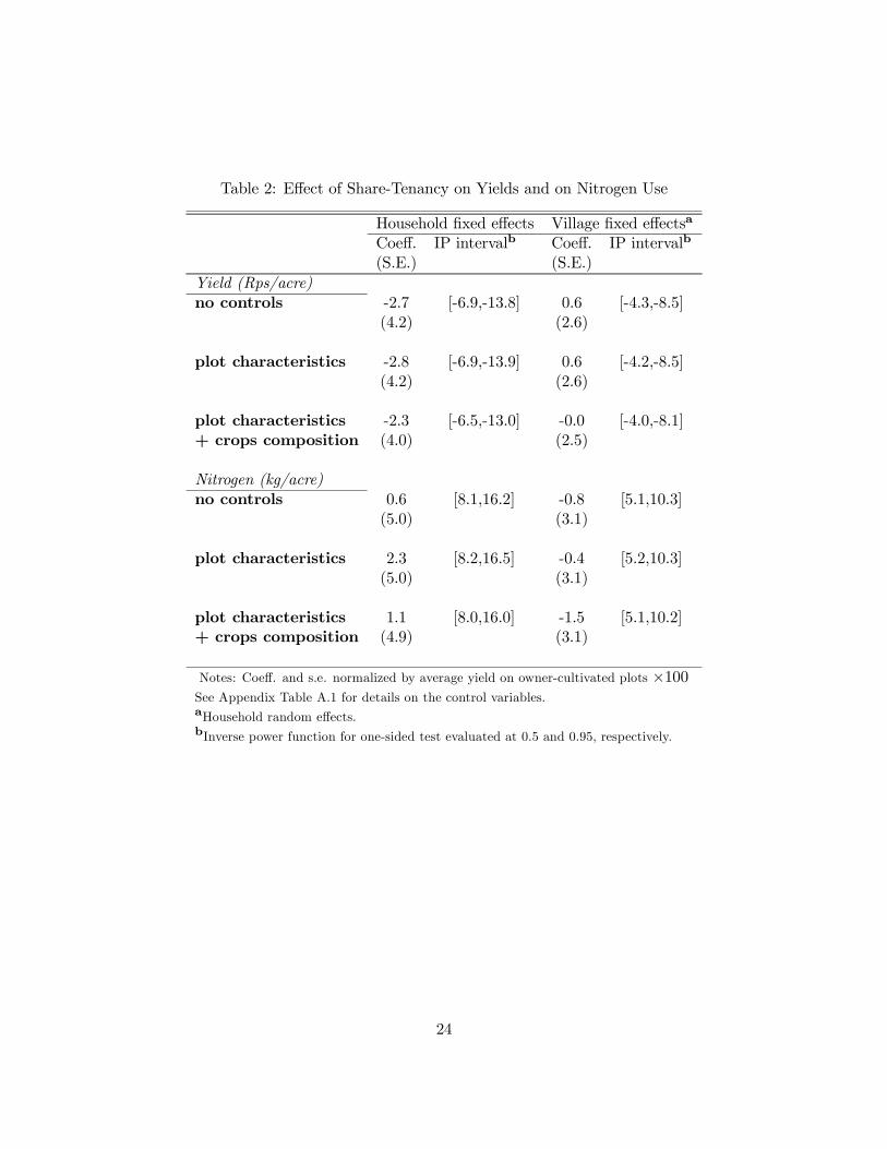
Table 2: Effect of Share-Tenancy on Yields and on Nitrogen Use

Household fixed effects Village fixed effectsa

Coeff. IP intervalb Coeff. IP intervalb

(S.E.) (S.E.)Yield (Rps/acre)no controls -2.7 [-6.9,-13.8] 0.6 [-4.3,-8.5]

(4.2) (2.6)

plot characteristics -2.8 [-6.9,-13.9] 0.6 [-4.2,-8.5](4.2) (2.6)

plot characteristics -2.3 [-6.5,-13.0] -0.0 [-4.0,-8.1]+ crops composition (4.0) (2.5)

Nitrogen (kg/acre)no controls 0.6 [8.1,16.2] -0.8 [5.1,10.3]

(5.0) (3.1)

plot characteristics 2.3 [8.2,16.5] -0.4 [5.2,10.3](5.0) (3.1)

plot characteristics 1.1 [8.0,16.0] -1.5 [5.1,10.2]+ crops composition (4.9) (3.1)

Notes: Coeff. and s.e. normalized by average yield on owner-cultivated plots ×100See Appendix Table A.1 for details on the control variables.aHousehold random effects.bInverse power function for one-sided test evaluated at 0.5 and 0.95, respectively.

24

Table 3: Effect of Share-Tenancy on Labor Use

Household fixed effects Village fixed effectsa

Coeff. IP intervalb Coeff. IP intervalb

Type of Labor (hrs/acre) (S.E.) (S.E.)

All agricultural tasksFamily -6.4 [-10.4,-20.7] 5.3 [-9.0,-18.1]

(7.0) (5.4)

Family + hired 0.8 [-12.2,-24.4] 8.0 [-9.4,-18.8](7.7) (5.5)

Excluding harvesting/threshingFamily -1.9 [-12.8,-25.6] 6.1 [-10.4,-20.9]

(8.3) (6.2)

Family + hired 0.2 [-13.3,-26.6] 6.4 [-10.6,-21.3](8.5) (6.3)

Notes: Coefficients and standard errors from logarithmic specifications are converted to percentage

changes. All specifications include plot characteristics and crop composition.aHousehold random effects.bInverse power function for one-sided test evaluated at 0.5 and 0.95, respectively.

25

Table 4: Landlord Supervision and Yields

Mean (s.d.) (1) (2) (3) (4) (5)Sharecropped plota 0.28 -4.4 -5.0 -4.8 -2.5 -4.8

(4.8) (4.9) (5.1) (4.9) (5.2)

Supervised (mci > k) 0.65 28.1 27.4 29.4 25.8 26.4(10.9) (11.0) (11.2) (11.0) (11.3)

Tenant characteristicsRecent (≤ 3 yrs.) 0.29 -5.7 -1.4

(10.2) (11.1)

Relative of landlord 0.34 10.0 20.0(10.3) (11.4)

Contract termsOutput share 0.48 -0.7 -1.0

(0.11) (0.8) (0.8)

Input share (average) 0.72 0.3 0.5(0.26) (0.4) (0.4)

Landlord gives credit 0.22 -4.7 -9.1(16.0) (16.5)

Landlord characteristicsLog of landholdings 5.78 0.050 0.073

(1.64) (0.040) (0.043)

Owns a tractor 0.32 12.7 11.0(12.4) (12.6)

Owns a tubewell 0.21 13.6 14.8(14.8) (14.9)

Notes: All regressions include plot characteristics, crop composition variables, and household

fixed effects. Coeff. (s.e.) normalized by average yield on unsupervised sharecropped plots ×100unless otherwise noted. Sample size is 1256 plots.aCoefficient renormalized by average yield on owner-cultivated plots. Mean of this variable is taken

over all plots in the sample; means of other variables are taken over 351 sharecropped plots.

26

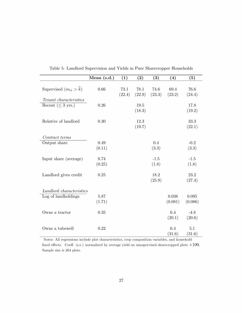
Table 5: Landlord Supervision and Yields in Pure Sharecropper Households

Mean (s.d.) (1) (2) (3) (4) (5)

Supervised (mci > k) 0.66 73.1 78.1 74.6 69.4 76.6(22.4) (22.9) (23.3) (23.2) (24.4)

Tenant characteristicsRecent (≤ 3 yrs.) 0.26 19.5 17.8

(18.3) (19.2)

Relative of landlord 0.30 12.3 33.3(19.7) (22.1)

Contract termsOutput share 0.49 0.4 -0.2

(0.11) (3.3) (3.3)

Input share (average) 0.74 -1.5 -1.5(0.25) (1.8) (1.8)

Landlord gives credit 0.25 18.2 23.2(25.9) (27.4)

Landlord characteristicsLog of landholdings 5.87 0.038 0.095

(1.71) (0.081) (0.086)

Owns a tractor 0.35 6.4 -4.8(20.1) (20.6)

Owns a tubewell 0.22 6.4 5.1(31.6) (31.6)

Notes: All regressions include plot characteristics, crop composition variables, and household

fixed effects. Coeff. (s.e.) normalized by average yield on unsupervised sharecropped plots ×100.Sample size is 264 plots.

27

Table 6: Multinomial Logit Model of Contract Choice

(1) (2)Mean (s.d.) FR MS FR MS

Landless tenant 0.54 -1.33* 0.33 -1.30* 0.27(0.45) (0.40) (0.45) (0.40)

Plot outside landlord’s village 0.14 0.16 -1.29* 0.23 -1.26*(0.49) (0.44) (0.47) (0.45)

Landlord characteristicsLog of landholdings 3.96 -0.09 0.43

(1.43) (0.24) (0.25)

Owns a tractor 0.11 -0.13 -1.03(0.72) (0.65)

Owns a tubewell 0.10 1.08 0.96(0.72) (0.61)

Note: Robust standard errors adjusted for village-level clustering in parentheses. Asterisk

denotes significance at above the 0.01 level. Each equation also includes the other plot

characteristics (see appendix), dummies for seasonal leases, and province dummies. The

Omitted category is the standard (unmonitored) share-contract.

28