Loughborough UniversityInstitutional Repository

The importance of unsteadyaerodynamics to road vehicle

dynamics

This item was submitted to Loughborough University's Institutional Repositoryby the/an author.

Citation: FULLER, J. ... et al, 2013. The importance of unsteady aerody-namics to road vehicle dynamics. Journal of Wind Engineering and IndustrialAerodynamics, 117, pp.1-10.

Additional Information:

• This is the author's version of a work that was accepted for publicationin Journal of Wind Engineering and Industrial Aerodynamics. Changesresulting from the publishing process, such as peer review, editing, correc-tions, structural formatting, and other quality control mechanisms maynot be reflected in this document. Changes may have been made to thiswork since it was submitted for publication. A definitive version wassubsequently published in Journal of Wind Engineering and IndustrialAerodynamics, 117, 2013, DOI: 10.1016/j.jweia.2013.03.006

Metadata Record: https://dspace.lboro.ac.uk/2134/15959

Version: Accepted for publication

Publisher: c© Elsevier

Rights: This work is made available according to the conditions of the Cre-ative Commons Attribution-NonCommercial-NoDerivatives 4.0 International(CC BY-NC-ND 4.0) licence. Full details of this licence are available at:https://creativecommons.org/licenses/by-nc-nd/4.0/

Please cite the published version.

The importance of unsteady aerodynamics to road vehicle dynamics Joshua Fuller Matt Best Nikhil Garret Martin Passmore (corresponding author) Department of Aeronautical and Automotive Engineering, Loughborough University, Leicestershire, UK, LE11 3TU Tel: +44 (0)1509 227 264 Fax: +44 (0)1509 227 275 Email: ttmap@lboro.ac.uk Abstract This paper investigates the influence that different unsteady aerodynamic components have on a vehicle’s handling. A simulated driver and vehicle are subject to two time-dependent crosswinds, one representative of a windy day and the second an extreme crosswind gust. Initially a quasi-static response is considered and then 5 additional sources of aerodynamic unsteadiness, based on experimental results, are added to the model. From the simulated vehicle and driver, the responses are used to produce results based on lateral deviation, driver steering inputs and also to create a ‘subjective’ handling rating. These results show that the largest effects are due to the relatively low frequency, time-dependent wind inputs. The additional sources of simulated unsteadiness have much smaller effect on the overall system and would be experienced as increased wind noise and reduced refinement rather than a worsening of the vehicle’s handling. Keywords Unsteady Aerodynamics, Vehicle Dynamics, Driver Model, Crosswinds, Vehicle Handling Notation A – Frontal Area (m2) β – Yaw Angle (rad) CYFβ – Front side force coefficient gradient CCYβ – Rear side force coefficient gradient FYf – Front aerodynamic side force (N) FYr – Rear aerodynamic side force (N) ρ – air density (kg/m3) m – Vehicle mass (kg) IG – Vehicle inertia matrix (kgm2) Jsw – Steering column moment of inertia (kgm2) Bsw – Steering column damping (Nm/rad)

1. Introduction The aerodynamic development of production vehicles is typically done in isolation from the chassis, disregarding the effects of the unsteady aerodynamics on the handling of the vehicle. Equally, aerodynamic testing generally uses steady-state conditions, despite the on-road environment being highly unsteady and the vehicle stability is assessed based on the steady state yaw moment gradient which is compared to competitor vehicles and company defined design targets. The yaw moment arises because when in a yawed flow there are low pressure regions on the front leeside and at the rear windward edge Howell (1996). These create a positive yaw moment gradient that turns the cars further away from the wind source, creating an unstable situation. The effects of the interaction between the vehicle aerodynamics and handling can only be tested with prototype vehicles and by this stage of development, the main body design is finalised and any possible geometry or shape modifications are very limited in scope. If aerodynamic induced handling problems are found, it is possible to partially mask them with changes to the suspension or by adding small flow control features such as spoilers or strakes; two examples of cars where these measures have been needed are the Mk1 Audi TT and Ford Sierra. It would be desirable to have a better understanding of the unsteady aerodynamics that cause handling issues; this could lead to preventative body shape features being included within the initial designs and allow aerodynamic and handling tests during the vehicle development process to be more targeted at the problematic conditions preventing the need for a reactive approach when problems arise. The onset wind conditions experienced during normal driving, are highly unsteady and contain a range of different inputs and frequencies: changing vehicle speed, pitch and yaw angles, changes in weather including windspeed, direction and gusts as well as the influence of local topography, buildings, trees, etc, and other road users. The unsteady aerodynamics of bluff and quasi-streamlined road vehicles is an area of interest with a large and expanding body of research. Instantaneous flow fields around statically mounted vehicles can be significantly different from the time averaged flow field, first shown by Bearman (1984) and subsequently by Sims-Williams et al (2001), Duell and George (1993) and Gilhome et al (2001) among others, on fastbacks, square backs and notchbacks respectively. To investigate the effect of unsteady onset flow yaw angles a range of methods have been employed, including oscillating onset winds, crosswind gust generators and models that oscillate or move across a windtunnel (Chadwick et al, 2001, Garry and Cooper, 1986, Mansor and Passmore, 2008, Ryan and Dominy, 1998, Theissen et al 2011, Wojciak et al 2011). These methods have produced conflicting results, in some case showing aerodynamic coefficients measured under transient conditions to be larger than those measured on a static model and in others the same or smaller. There is also evidence of flow field hysteresis, Guilmineau and Chometon (2008); periodic features within the flow field suppressing frequencies within the unsteady onset wind, Schröck et al (2009) and different response times from different flow structures, Ryan and Dominy (1998), but there is no comprehensive description of the flow field differences. Research into the interaction between vehicle aerodynamics and handling has only seen sporadic interest over the past 30 years (Aschwanden et al, 2008, Baker, 1993, Juhlin and Eriksson, 2004, Klein and Hogue, 1980, Macadam et al, 1990, Schrock et al, 2011, Wullimeit et al, 1988) but none considers which components of the unsteady onset flow or resultant flow fields are important to the handling of the vehicle. Goetz (1995) states that inputs in the frequency range 0.5-2Hz affect the vehicle due to interactions with the suspension resonances, Wagner and Wiedemann (2002) also showed that this frequency range produced the worst response from a driver, and that higher frequencies are a NVH (noise, vibration and harshness) problem. Amongst the published work, there is a general consensus that good subjective assessments of a vehicle’s handlings in crosswinds correlate with low vehicle yaw rates and yaw rate RMS. Lateral deviation due to crosswinds is only of secondary importance in driver subjective assessments although important for lane discipline, directional control and refinement. This paper will use experimental aerodynamic results in a simulated driver and vehicle model to assess the importance of the different sources of crosswind aerodynamic unsteadiness on vehicle handling. The vehicle

model was subjected to two onset wind conditions creating unsteady side force and yaw moments, one representing naturally occurring crosswinds typically found on a motorway and the second an extreme and sudden crosswind gust with an onset flow yaw angle of 30º. To these onset conditions, different sources of unsteadiness were applied:

• Difference between a steady-state and transient yaw angle • Time delay between the front and rear of the vehicle • Yaw moment hysteresis • Instantaneous unsteadiness in side force • Frequency dependent yaw moment magnification

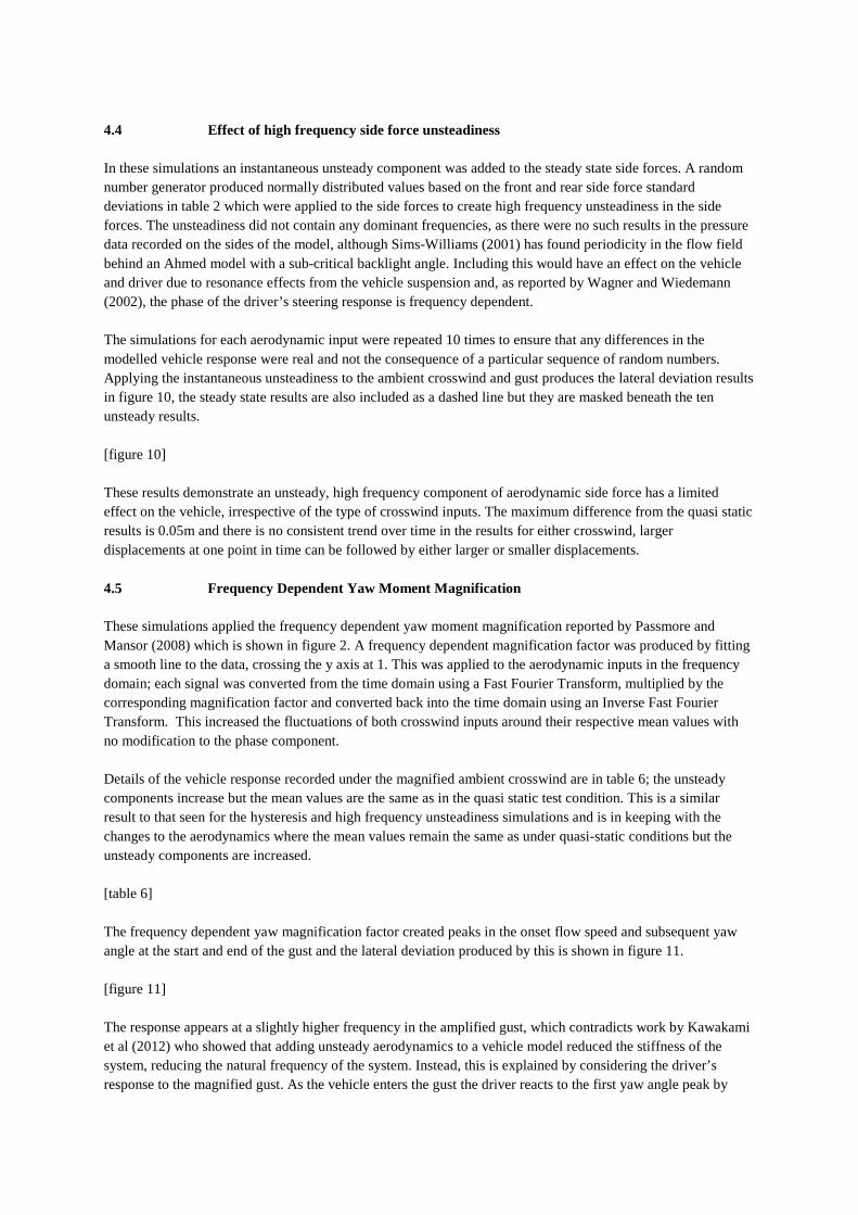
2 Vehicle Aerodynamics The aerodynamic loads used in the simulated vehicle model were based on experimental results collected in the Loughborough University ¼ scale windtunnel using a Davis model, Davis (1982), which is shown in figure 1; all the edges having a 20mm radius. [figure 1] The windtunnel is an open circuit design with a closed working section which has a fixed floor, boundary layer thickness of 60mm and a freestream turbulence intensity of 0.2%; further details are in Johl et al (2004). The model was mounted 40mm above the ground plane of the windtunnel to the underfloor balance via a Ø20mm shaft from the centre of the model. The balance is accurate to ±0.12N in drag, ±0.52N in side force and ±0.045Nm in yaw moment. This gives accuracy in the lateral coefficients of ±3% or side force and ±2% in yaw moment; as will be seen in the results, this level of error is insignificant compared to the variations that occur in these parameters due to other factors. Data was sampled for 20s to record a repeatable mean within ±1 count. Steady-state data was collected using the underfloor balance at static yaw angles in steps of 2º between β= ±30º at a tunnel speed of 40m/s, giving a Reynolds number, based on model length, of 1.7 x106. This value is above the typical lower threshold of Reynolds number independence for scale model tests of 1x106, and for this model a simple Reynolds sweep shows that the aerodynamic coefficients become reasonably Reynolds number independent above 1.3x106. However it is acknowledged that when applying this data in a full scale vehicle simulation there is likely to be some Reynolds number dependency particularly in the coefficients in extreme conditions. The loads were corrected for model blockage using the MIRA blockage correction, Carr (1982), and converted to coefficients using the standard equations and SAE coordinate system. The steady-state front and rear side force and yaw moment coefficients produce linear results, r2>0.97, with gradients in table 1. [table 1] The flow fields around the model are naturally unsteady, causing instantaneous variations from the mean values of the aerodynamic loads acting on the model. The standard deviation of the side forces was found from high frequency, surface pressure measurements on the two sides of the model. The model was mounted in the windtunnel in the same way as for the steady-state force measurements, with 63 pressure tappings on each side of the model connected to two 64 channel miniature pressure scanners via lengths of flexible plastic tubing. Data was collected at 260Hz for 32 seconds, giving 8192 data points at each pressure tapping. The pressure transducer is accurate to 0.9mm H2O, meaning that the uncertainty in the readings is of the order 1 – 2%, and was post processed to remove distortions caused by the tubing; these were dominated by a resonance at 95Hz and an increasing phase lag at higher frequencies. Area weighted side forces were calculated at each instantaneous time step and at each yaw angle. The mean area weight side force gradient was 66% of the value found using the balance. It was lower due to the finite number of tappings available and the steep surface

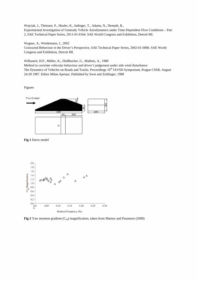
pressure gradients that are found on the curved edges of the model. The resolution is sufficient to capture the information required to interpret the flow field but insufficient to calculate the true side force gradient. The instantaneous side forces had a normal distribution with a standard deviation that increased as the mean value also increased. The standard deviations are given in table 2 as a percentage of the mean front side force values and show that the standard deviation of the rear side force is much larger than the front side force. [table 2] Mansor and Passmore (2008) mounted the same Davis model on a sprung oscillating model rig, and used the model response to derive the yaw moment gradient. When compared to the steady-state results the oscillating model results were larger and frequency dependent, as shown in figure 2. This potentially questions the validity and usefulness of steady state results as a basis for vehicle stability assessments and these results will be used in the simulations to determine if a frequency dependent, yaw moment magnification has a significant effect on the vehicle model’s response. [figure 2] 3. Vehicle and Driver Models The vehicle is modelled as a six degree of freedom, rigid body with tyre and aerodynamic force inputs on a flat road, as in Figure 3. [figure 3] The principal equations of motion for the vehicle of mass m and inertia IG are:

( )1iG G

iv F mv

mω

= − × ∑

Eq. 1

( ) ( )1i iG G

iI r F Iω ω ω−

= × − × ∑

Eq.2

governing triaxial translational velocities vG and rotational velocities ω, in response to the set of tyre,

suspension and aerodynamic forces F acting at positions r from the CG for each of the tyre contact patches (i).

Tyre forces are found from a combined slip Pacejka formula (see for example Milliken and Milliken (1995)) based on lateral and longitudinal slips computed from the velocity vectors at the contact patches, C. These forces vary appropriately with vertical load, found assuming a linear spring-damper suspension, Fs, compensated by suspension link forces assumed to act at static roll centres. Four wheel spin degrees of freedom are modelled, driven by input drive torque τ shared equally at the front wheels, and reacted by longitudinal forces Fxi, and a nominal road drag. A full description of the tyre model is available in Gordon and Best (2006). The vehicle parameters are nominal, consistent with a medium sized passenger vehicle, sourced from Dixon (1996). The aerodynamic inputs were limited to the front and rear side forces and yaw moment but the effects of lift, drag, roll and pitch have not been considered. Whilst, including these would increase the accuracy of the simulation, by including effects such as roll steer and changes in tyre load caused by lift, notably Howell and Le Good (1999) identified a link between higher rear lift and reduced vehicle straight line stability, the simulations in this paper are focused on primary crosswind effects. The instantaneous front and rear side force coefficients were calculated by multiplying the side force coefficient gradients, CYFβ and CYRβ, by the yaw angle, β, which was found from the vector sum of the crosswind and

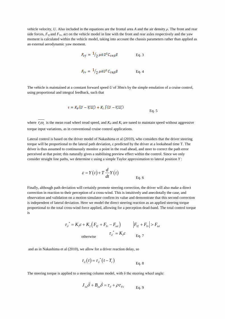
vehicle velocity, U. Also included in the equations are the frontal area A and the air density ρ. The front and rear side forces, FYf and FYr, act on the vehicle model in line with the front and rear axles respectively and the yaw moment is calculated within the vehicle model, taking into account the chassis parameters rather than applied as an external aerodynamic yaw moment.

Eq. 3

Eq. 4 The vehicle is maintained at a constant forward speed U of 30m/s by the simple emulation of a cruise control, using proportional and integral feedback, such that

Eq. 5

where r irω is the mean road wheel tread speed, and KP and KI are tuned to maintain speed without aggressive

torque input variations, as in conventional cruise control applications. Lateral control is based on the driver model of Nakashima et al (2010), who considers that the driver steering torque will be proportional to the lateral path deviation, ε predicted by the driver at a lookahead time T. The driver is thus assumed to continuously monitor a point in the road ahead, and steer to correct the path error perceived at that point; this naturally gives a stabilising preview effect within the control. Since we only consider straight line paths, we determine ε using a simple Taylor approximation to lateral position Y :

( ) ( )dY t T Y tdt

ε = + Eq. 6

Finally, although path deviation will certainly promote steering correction, the driver will also make a direct correction in reaction to their perception of a cross-wind. This is intuitively and anecdotally the case, and observation and validation on a motion simulator confirm its value and demonstrate that this second correction is independent of lateral deviation. Here we model the direct steering reaction as an applied steering torque proportional to the total cross-wind force applied, allowing for a perception dead-band. The total control torque is

( )*1 2 Yf Yr tolK K F F Fδτ ε= + + −

Yf Yr tolF F F+ >

otherwise *

1Kδτ ε= Eq. 7

and as in Nakashima et al (2010), we allow for a driver reaction delay, so

( ) ( )*rt t Tδ δτ τ= −

Eq. 8

The steering torque is applied to a steering column model, with δ the steering wheel angle:

sw sw FxJ B δδ δ τ ρτ+ = + Eq. 9

τFx is the reaction torque, calculated from the tyre lateral forces, taking into account pneumatic and mechanical

trails, caster and kingpin inclinations, and ρ is the steered wheel to steering wheel magnification factor. 3.1 Onset Wind Conditions Two crosswind conditions were simulated, representing naturally occurring, windy conditions and an extreme gust. The crosswinds were modelled as a wind at 90º to the initial direction of travel of the modelled vehicle. The natural ambient onset conditions (figure 4a) were generated using an implementation of the Dryden filter, which uses an input of band-limited white noise and the output then closely matches power spectral density relationships found for ambient wind, Maclean (1976). Appropriate length scales and turbulence ratios were found in Cooper (1984). The resulting power spectral density (figure 4b) illustrates that the bulk of the energy is below 1Hz. The simulated crosswind profile, in figure 4a, had a mean velocity of -4.3m/s, based on Ingram 1978. This was the mean wind speed measured by the Met Office over 9 years, from 1966 to 1975, at 10m. [figure 4] The gust is a single, extreme crosswind that creates a 30º yaw angle and lasts 2 seconds with the onset and decay ramps each lasting 0.1s, shown in figure 5. This gust input is not a realistic situation, yaw angles larger than ±10º are very rare, Carlino et al 2007, but is similar to the crosswind tests where a car is driven in front of an array of fans used by some car manufactures and reported by Klein and Hogue (1980) and Macadam et al (1990). [figure 5] 3.2 Driver Model Validation The intention was to perform the entire study in simulation only but initial results showed the vehicle response was very sensitive to the driver parameters hence it was imperative to find reasonable values for these. These were determined using real driver data collected using a motion simulator; three drivers were subject to a crosswind, their responses were recorded and the modelled driver parameters were fitted to these. The simulator uses a commercially available six-DOF electric motion platform with a bandwidth of 20Hz and maximum excursion of the order ±0.4m and ±25° in the translational and rotational degrees of freedom – complete specifications available on the Moog website. A DC motor provides feedback through the steering column with a maximum torque of 30Nm and a bandwidth of 20Hz; the visual system comprises three 24” LCD screens providing a wide-angle forward view. The vehicle model described earlier in this section was implemented in MATLAB/Simulink with an integrator step size of 1ms.The participants were asked to drive along a straight motorway-style track and maintain their position within a lane while travelling at a fixed speed of 110 km/h (30 m/s). The extreme crosswind gust was repeatedly applied to the vehicle at random intervals and the vehicle states and driver steering input were recorded for each run. Each participant produced a different response to the crosswind gust so only the results from the most consistent driver were used to tune the driver model parameters. Noise was removed from the data with a low pass filter and the driver model was optimised using the genetic algorithm optimisation procedure in Matlab considering the front wheel steering angle. A comparison of the recorded data and the optimised driver model is in figure 6, also demonstrated is the influence of the direct driver component, K2.

[figure 6] This modelled response gives good agreement with the data collected from the motion simulator and shows the value of the direct feedback term to the driver model. The optimised driver parameters used in the simulations are in table 3. [table 3] Using this method to collect data for the driver model optimisation meant each participant was repeatedly exposed to the crosswind gust, thereby, in theory, learning what to expect. This was unavoidable but there is no trend within the data to indicate an improving response over time. Furthermore, real world tests driving a vehicle across a crosswind generator suffer from the same problem but with the greater problem of the approaching fans being a visual trigger to the upcoming disturbance. Klein and Hogue (1980) recommend testing under naturally occurring crosswinds however using this type of testing in this instance would not have been suitable for creating a repeated test condition for use in the driver parameter tuning. 4. Results From the data generated by simulating the driver and vehicle in the crosswinds with each source of unsteadiness, the analysis will consider the lateral deviation of the vehicle and a synthesised subjective handling rating. Lateral deviation is driver dependent and is considered from a safety and refinement point of view as there is no point having an easily controlled car if the lateral deviation is large. Although different drivers have different responses to crosswinds, Macadam et al (1990) found different driver’s subjective ratings were consistent hence this is used to remove the driver dependency from the results. The tests are summarised in table 4 with details of how the unsteadiness is implemented given prior to the results. The standard test case uses a quasi-static aerodynamic input and the subsequent modifications to the unsteadiness are compared to these results. The lateral deviation caused by each test case will be discussed in each section and the subjective ratings are in section 4.6. [table 4] 4.1 Effect of unsteady onset conditions This compares the model’s response to unsteady crosswind inputs with a constant crosswind equal to the mean value. The differences in the lateral deviation of the vehicle under naturally occurring crosswinds is in figure 7. With a steady state input the driver settles the vehicle at a consistent lateral deviation of 0.08m from the initial starting position. The driver does not return to 0 displacement because the proportional control system used in the driver model produces a steady state error. Under the unsteady crosswind the vehicle does not settle to a constant lateral deviation, however the mean lateral deviation closely matches that from the steady state crosswind. [figure 7] The mean lateral displacement in the ambient crosswind is 0.067m, which closely matches the steady state lateral displacement of 0.08m, but the maximum difference between the two sets of results is 0.22m, which is approaching a displacement that could lead to problems staying in lane and may be interpreted as poor vehicle refinement. The same comparison was carried out with the crosswind gust; although this is a rather arbitrary case with the mean crosswind dependent on the total length of time before and after the gust. The results are in figure 8, the

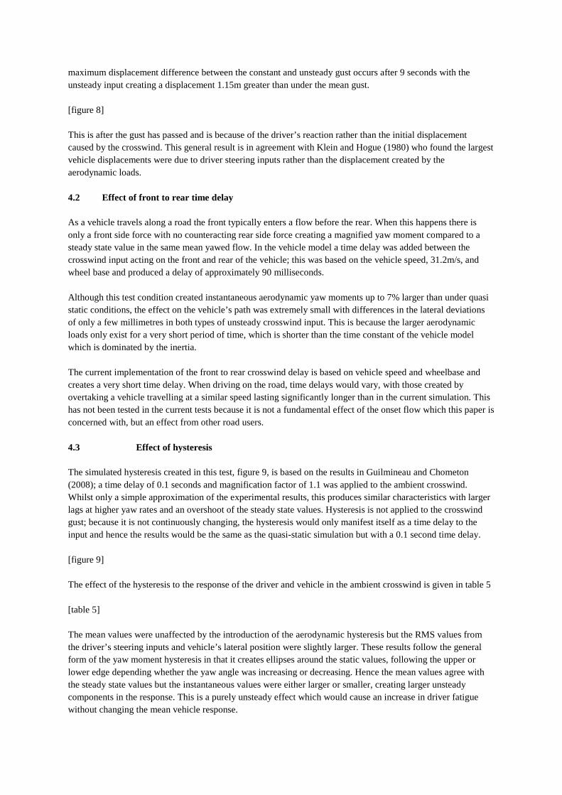
maximum displacement difference between the constant and unsteady gust occurs after 9 seconds with the unsteady input creating a displacement 1.15m greater than under the mean gust. [figure 8] This is after the gust has passed and is because of the driver’s reaction rather than the initial displacement caused by the crosswind. This general result is in agreement with Klein and Hogue (1980) who found the largest vehicle displacements were due to driver steering inputs rather than the displacement created by the aerodynamic loads. 4.2 Effect of front to rear time delay As a vehicle travels along a road the front typically enters a flow before the rear. When this happens there is only a front side force with no counteracting rear side force creating a magnified yaw moment compared to a steady state value in the same mean yawed flow. In the vehicle model a time delay was added between the crosswind input acting on the front and rear of the vehicle; this was based on the vehicle speed, 31.2m/s, and wheel base and produced a delay of approximately 90 milliseconds. Although this test condition created instantaneous aerodynamic yaw moments up to 7% larger than under quasi static conditions, the effect on the vehicle’s path was extremely small with differences in the lateral deviations of only a few millimetres in both types of unsteady crosswind input. This is because the larger aerodynamic loads only exist for a very short period of time, which is shorter than the time constant of the vehicle model which is dominated by the inertia. The current implementation of the front to rear crosswind delay is based on vehicle speed and wheelbase and creates a very short time delay. When driving on the road, time delays would vary, with those created by overtaking a vehicle travelling at a similar speed lasting significantly longer than in the current simulation. This has not been tested in the current tests because it is not a fundamental effect of the onset flow which this paper is concerned with, but an effect from other road users. 4.3 Effect of hysteresis The simulated hysteresis created in this test, figure 9, is based on the results in Guilmineau and Chometon (2008); a time delay of 0.1 seconds and magnification factor of 1.1 was applied to the ambient crosswind. Whilst only a simple approximation of the experimental results, this produces similar characteristics with larger lags at higher yaw rates and an overshoot of the steady state values. Hysteresis is not applied to the crosswind gust; because it is not continuously changing, the hysteresis would only manifest itself as a time delay to the input and hence the results would be the same as the quasi-static simulation but with a 0.1 second time delay. [figure 9]

The effect of the hysteresis to the response of the driver and vehicle in the ambient crosswind is given in table 5 [table 5] The mean values were unaffected by the introduction of the aerodynamic hysteresis but the RMS values from the driver’s steering inputs and vehicle’s lateral position were slightly larger. These results follow the general form of the yaw moment hysteresis in that it creates ellipses around the static values, following the upper or lower edge depending whether the yaw angle was increasing or decreasing. Hence the mean values agree with the steady state values but the instantaneous values were either larger or smaller, creating larger unsteady components in the response. This is a purely unsteady effect which would cause an increase in driver fatigue without changing the mean vehicle response.

4.4 Effect of high frequency side force unsteadiness In these simulations an instantaneous unsteady component was added to the steady state side forces. A random number generator produced normally distributed values based on the front and rear side force standard deviations in table 2 which were applied to the side forces to create high frequency unsteadiness in the side forces. The unsteadiness did not contain any dominant frequencies, as there were no such results in the pressure data recorded on the sides of the model, although Sims-Williams (2001) has found periodicity in the flow field behind an Ahmed model with a sub-critical backlight angle. Including this would have an effect on the vehicle and driver due to resonance effects from the vehicle suspension and, as reported by Wagner and Wiedemann (2002), the phase of the driver’s steering response is frequency dependent. The simulations for each aerodynamic input were repeated 10 times to ensure that any differences in the modelled vehicle response were real and not the consequence of a particular sequence of random numbers. Applying the instantaneous unsteadiness to the ambient crosswind and gust produces the lateral deviation results in figure 10, the steady state results are also included as a dashed line but they are masked beneath the ten unsteady results. [figure 10] These results demonstrate an unsteady, high frequency component of aerodynamic side force has a limited effect on the vehicle, irrespective of the type of crosswind inputs. The maximum difference from the quasi static results is 0.05m and there is no consistent trend over time in the results for either crosswind, larger displacements at one point in time can be followed by either larger or smaller displacements. 4.5 Frequency Dependent Yaw Moment Magnification These simulations applied the frequency dependent yaw moment magnification reported by Passmore and Mansor (2008) which is shown in figure 2. A frequency dependent magnification factor was produced by fitting a smooth line to the data, crossing the y axis at 1. This was applied to the aerodynamic inputs in the frequency domain; each signal was converted from the time domain using a Fast Fourier Transform, multiplied by the corresponding magnification factor and converted back into the time domain using an Inverse Fast Fourier Transform. This increased the fluctuations of both crosswind inputs around their respective mean values with no modification to the phase component. Details of the vehicle response recorded under the magnified ambient crosswind are in table 6; the unsteady components increase but the mean values are the same as in the quasi static test condition. This is a similar result to that seen for the hysteresis and high frequency unsteadiness simulations and is in keeping with the changes to the aerodynamics where the mean values remain the same as under quasi-static conditions but the unsteady components are increased. [table 6] The frequency dependent yaw magnification factor created peaks in the onset flow speed and subsequent yaw angle at the start and end of the gust and the lateral deviation produced by this is shown in figure 11. [figure 11] The response appears at a slightly higher frequency in the amplified gust, which contradicts work by Kawakami et al (2012) who showed that adding unsteady aerodynamics to a vehicle model reduced the stiffness of the system, reducing the natural frequency of the system. Instead, this is explained by considering the driver’s response to the magnified gust. As the vehicle enters the gust the driver reacts to the first yaw angle peak by

adding more steering angle than under steady state conditions, which is maintained to react the crosswind gust. Once the gust passes, the vehicle steers more quickly and the driver is aware that the course of the vehicle is wrong sooner than under the steady state response. This creates the faster reaction but the driver cannot change the steering angle fast enough and the lateral deviation is larger. 4.6 Subjective Ratings Synthesised subjective ratings are calculated for each type of aerodynamic input to explore which would create the biggest difference in the feel of the vehicle independently of the driver model parameters. These are calculated using equation 7, taken from Macadam et al (1990), which is an empirical equation that links the subjective handling rating of a vehicle to normalised vehicle yaw rate RMS with small values indicating a better handling vehicle.

Subjective Rating = 2.488 + 2.464x Eq. 11

Where ‘x is the normalised yaw rate RMS, equation 12. It is important to note that the absolute RMS yaw rates for the ambient crosswind and gust conditions were different.

Eq. 12

[table 7] For both types of crosswind input most of the subjective ratings are very similar, the only significant change is caused by replacing the unsteady crosswind with an equivalent mean value which for both types of wind creates a much better subjective response. Also common to both types of crosswind input, the frequency dependent yaw moment magnification created the worst subjective rating, however this was only slightly worse than the other sources of aerodynamic unsteadiness which only cause very small changes to the subjective rating that are likely to be insignificant. This similar trends in the results from the two different crosswind inputs agrees with the findings of Klein and Hogue (1980) who found the subjective ratings of cars were independent of onset flow yaw rate. 4.7 Discussion Both the lateral deviation and subjective results show the most influential source of unsteadiness in the lateral aerodynamics on vehicle handling is the relatively large scale changes created by testing in time varying, onset wind conditions rather than under steady state conditions. The hysteresis, instantaneous unsteadiness, frequency dependent yaw moment magnification and time delay only add small scale effects on top of the mean vehicle response which is dominated by the unsteady onset wind. The effects of these sources of unsteadinesses are typically only seen in the unsteady components of the results and are, at most, an order of magnitude smaller than the effects from the unsteady onset crosswinds. This demonstrates the importance of unsteady wind inputs, indicating that vehicle development should give greater consideration to the effects of relatively large scale onset flow unsteadiness but that with current vehicles further sources of unsteadiness may be unimportant to vehicle handling. This agrees with Goetz (1995) who showed that relatively low frequency unsteady inputs between 0.5-2Hz had the largest effect on the unsteady response of the vehicle. The further sources of unsteadiness added to the basic large scale unsteadiness are higher frequency and are important for vehicle NVH and refinement, which directly influence a customer’s perception of quality. Increased aerodynamic unsteadiness will also lead to greater driver fatigue caused by the larger steering inputs and greater wind noise, as in Peric et al (1997), which would lead to a worsening of the driver response. In reality, unlike in this paper, any of the further sources of unsteadiness are fundamentally linked to the larger scale onset flow and any vehicle testing in unsteady conditions will inherently include these effects whether

intentionally or not. Better understanding of these effects will continue to be beneficial as by understanding how they manifest themselves, design features that mitigate or take advantage of them will be developed, leading to improved refinement and possibly new avenues in vehicle design. 5. Conclusions This paper shows the development of a vehicle model and the effect of various unsteady aerodynamic inputs on the vehicle’s handling. The results lead to the conclusion that the most important of an unsteady crosswind for vehicle handling are the large scale changes in the onset wind. The extra sources of unsteadiness do modify the side forces but these affect the refinement of the vehicle rather than the handling. These extra sources of unsteadiness are a fundamental part of the unsteady onset flow so any development work carried out in these conditions will inherently consider these also. By gaining a better understanding of these, vehicle refinement could be improved as designers learn how to prevent or lessen these effects. 6. Acknowledgements The authors would like to thank Rob Hunter for his help with the windtunnel testing and Dan Wood for developing the tubing correction used to find the instantaneous pressure coefficients and for being one of the test drivers on the motion simulator. 7. References Aschwanden P, Müller, J., Travaglio, G.C., Schöning, T. 2008 The Influence of Motion Aerodynamics on the Simulation of Vehicle Dynamics. SAE Technical Paper Series, 2008-01-0657. SAE World Congress and Exhibition, Detroit MI. Baker, C.,J. 1993 The Behaviour of Crosswinds in Unsteady Crosswinds, Journal of Wind Engineering and Industrail Aerodynamics, Vol 49, Pages 439-448 Bearman, P.W., 1984 Some Observations on Road Vehicle Wakes. SAE Technical Paper Series, 840301. SAE World Congress and Exhibition, Detroit MI. Carr GW. 1982 Correlation of Aerodynamic Force Measurements in MIRA and Other Automotive Wind Tunnels. SAE Technical Paper Series, 820374. SAE World Congress and Exhibition, Detroit MI. Chadwick, A., Garry, K., Howell, J., 2001 Transient Aerodynamic Characteristics of Simple Vehicle Shapes by the Measurement of Surface Pressures., SAE Technical Paper Series, 2001-01-0876. SAE World Congress and Exhibition, Detroit MI. Cooper, R., K. 1984 Atmospheric turbulence with respect to moving ground vehicles Journal of Wind Engineering and Industrial Aerodynamics, Vol 17, Pages 215-238 Davis, J Wind Tunnel Investigation of Road Vehicle Wakes PhD thesis, London University, 1982

Dixon, J.C. 1996 Tires, Suspension and Handling (Ed 2, Appendix C) SAE Press. Duell, E. G, George, R.A. 1993 Measurements in the Unsteady Near Wakes of Ground Vehicle Bodies. SAE Technical Paper Series, 930298. SAE World Congress and Exhibition, Detroit MI. Garry, K.P., Cooper, K.R., 1986 Comparison of Quasi-Static and Dynamic Wind Tunnel Measurements on Simplified Tractor-Trailer Models, Journal of Wind Engineering and Industrial Aerodynamics, Vol 22, 185-194 Gilhome, B. R., Saunders, J. W., Sheridan, J., 2001 Time Averaged and Unsteady Near-Wake Analysis of Cars. SAE Technical Paper Series, 2001-01-1040. SAE World Congress and Exhibition, Detroit MI. Goetz, H. 1995 Crosswind facilities and test procedures. Society of Automotive Engineers. Gordon, T.J., and Best, M.C., 2006 On the Synthesis of Driver Inputs for the Simulation of Closed-loop Handling Manoeuvres, International Journal of Vehicle Design 2006 - Vol. 40, No.1/2/3 pp. 52 - 76. Guilmineau, E., Chometon, F., 2008 Numerical and Experimental Analysis of Unsteady Separated Flow behind an Oscillating Car Model. SAE Technical Paper Series, 2008-01-0738. SAE World Congress and Exhibition, Detroit MI. Howell, J.P., 1996 The side load distribution on a Rover 800 saloon car under crosswind conditions. Journal of Wind Engineering and Industrial Aerodynamics. Vol 60. Pages 139-153 Howell, J., Le Good, G., 1999 The Influence of Aerodynamic Lift on High Speed Stability, SAE Technical Paper Series, 1999-01-0651. SAE World Congress and Exhibition, Detroit MI. Ingram K.C. 1978 The wind averaged drag coefficient applied to heavy goods vehicles. DOE, DOT, TRRL Report SR392 1978. Johl, G., Passmore, M., Render, P., 2004 Design methodology and performance of an indraft wind tunnel The Aeronautical Journal, Vol 108, pages 465-473. Juhlin, M., Eriksson, P. 2004 A Vehicle Parameter Study on Crosswind Sensitivity of Buses, SAE Technical Paper Series, 2004-01-2612. SAE World Congress and Exhibition, Detroit MI. Kawakami, M., Norikazu, S., Aschwanden, p., Mueller, J.,Kato, Y., Nakagawa, M., Ono, E. Validation and Modelling of Transient Aerodynamic Loads acting on a Simplified Passenger Car Model in Sinusoidal Motion. SAE Technical Paper Series, 2012-01-0447. SAE World Congress and Exhibition, Detroit MI.

Klein, R. H, Hogue, J.R., 1980 Effects of Crosswinds on Vehicle Response – Full Scale Tests and Analytical Predictions SAE Technical Paper Series 800848. Passenger Car meeting, Dearborn June 1980. Le Good, G., Garry, K. P., 2004 On The Use of Reference Models in Automotive Aerodynamics, SAE Technical Paper Series, 2004-01-1308. SAE World Congress and Exhibition, Detroit MI. Macadam, C. C., Sayers, M.W., Pointer, J.D., Gleason, M. Crosswind Sensitivity of Passenger cars and the Influence of Chassis and Aerodynamic Properties on Driver Preferences. Vehicle System Dynamics, Vol 19, 1990, p201 - 236 Maclean, D. 1976 Gust load alleviation control systems. A feasibility study, Department of Transport Technology, Loughborough University, Report No.7606. Milliken, D.L., Milliken, W.F. 1995 Race Car Vehicle Dynamics, SAE International Nakashima, T., Tsubokura, M., Ikenaga, T. and Doi, Y. (2010) HPC-LES for Unsteady Aerodynamics of a Heavy Duty Truck in Wind Gust – 2nd Report : Coupled Analysis with Vehicle Motion, SAE Technical Paper Series, 2010-01-1021. SAE World Congress and Exhibition, Detroit MI. Mansor, S. and Passmore M.A., 2008 Estimation of bluff body transient aerodynamics using an oscillating model rig. Journal of Wind Engineering and Industrial Aerodynamics. Vol 96, Pages 1218-1231 Peric, C., Watkins, S., Lindqvist, E., 1997 Wind turbulence effects on aerodynamic noise with relevance to road vehicle interior noise. Journal of Wind Engineering and Industrial Aerodynamics, Vol 69 – 71, page 423 - 435 Ryan, A., Dominy, R.G., 1998 The Aerodynamic Forces induced on a Passenger Vehicle in Response to a Transient Cross-Wind Gust at a Relative incidence o 30º. SAE Technical Paper Series, 980392. SAE World Congress and Exhibition, Detroit MI. Schröck D; Widdecke, N; Wiedemann, J, 2009 Aerodynamic Response of a Vehicle Model to Turbulent Wind. 7th FKFS Conference Progress in Vehicle Aerodynamics and Thermal Management, October, 2009, Stuttgart Germany. Schröck, D., Krantz, W., Widdecke, N., Wiedemann, J., 2011 Unsteady Aerodynamic Properties of a Vehicle Model and their Effect on Driver and Vehicle under Side Wind Conditions, SAE Technical Paper Series, 2011-01-0154. SAE World Congress and Exhibition, Detroit MI. Sims-Williams, D.B., Dominy, R.G., Howell, J.P., 2001 An Investigation into Large Scale Unsteady Structures in the Wake of Real and Idealized Hatchback Car Models, SAE Technical Paper Series, 2001-01-1041. SAE World Congress and Exhibition, Detroit MI. Theissen. P., Wojciak, J., Heuler, K., Demuth, R., Indinger, T., Adams, N., Experimental Investigation of Unsteady Vehicle Aerodynamics under Time-Dependent Flow Conditions – Part 1. SAE Technical Paper Series, 2011-01-0177. SAE World Congress and Exhibition, Detroit MI.

Wojciak, J., Theissen. P., Heuler, K., Indinger, T., Adams, N., Demuth, R., Experimental Investigation of Unsteady Vehicle Aerodynamics under Time-Dependent Flow Conditions – Part 2, SAE Technical Paper Series, 2011-01-0164. SAE World Congress and Exhibition, Detroit MI. Wagner, A., Wiedemann, J., 2002 Crosswind Behaviour in the Driver’s Perspective, SAE Technical Paper Series, 2002-01-0086. SAE World Congress and Exhibition, Detroit MI. Willumeit, H.P., Müller, K., Dödlbacher, G., Matheis, A., 1988 Method to correlate vehicular behaviour and driver’s judgement under side wind disturbance The Dynamics of Vehicles on Roads and Tracks. Proceedings 10th IAVSD Symposium, Prague CSSR, August 24-28 1987. Editor Milan Apetaur. Published by Swet and Zeitlinger, 1988 Figures

Fig 1 Davis model

Fig 2 Yaw moment gradient (Cnβ) magnification, taken from Mansor and Passmore (2008)

Fig 3 Vehicle body free-body diagram

Fig 4 Simulated ambient crosswinds

Fig 5 Extreme crosswind gust

Fig 6 Validation of driver model

Fig 7 Lateral deviation caused by mean and unsteady ambient crosswinds

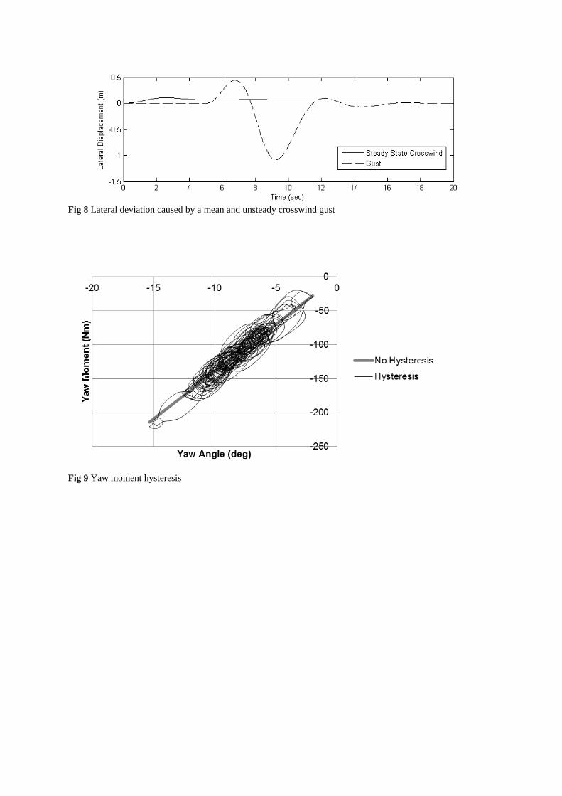
Fig 8 Lateral deviation caused by a mean and unsteady crosswind gust

Fig 9 Yaw moment hysteresis

Fig 10 a: ambient wind with unsteadiness, b: gust with unsteadiness. In both plots the steady state results are shown as a dashed line but it is hidden under the 10 unsteady results

Fig 11 Lateral deviation caused by magnified crosswind gust Tables Front Side Force Coefficient Gradient /º (CYFβ) 0.0194 Rear Side Force Coefficient Gradient /º (CYRβ) 0.0088 Yaw Moment coefficient Gradient /º 0.0055 Table 1, steady state lateral aerodynamic coefficients

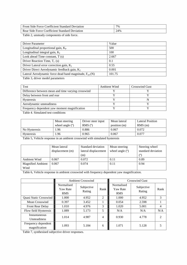
Table 2, unsteady components of side force. Driver Parameter Value Longitudinal proportional gain, KP 500 Longitudinal integral gain, KI 100 Look ahead Time constant, T (s) 2.667 Driver Reaction Time, Tr (s) 0.1 Driver Lateral error correction gain, K1 0.55 Driver Direct Aerodynamic feedback gain, K2 0.001 Lateral Aerodynamic force dead band magnitude, Ftol (N) 101.75 Table 3, driver model parameters Test Ambient Wind Crosswind Gust Difference between mean and time varying crosswind Y Y Delay between front and rear Y Y Hysteresis Y N Aerodynamic unsteadiness Y Y Frequency dependent yaw moment magnification Y Y Table 4. Simulated test conditions Mean steering

wheel angle (º) Driver steer input RMS (º)

Mean lateral position (m)

Lateral Position RMS (m)

No Hysteresis 1.96 0.886 0.067 0.072 Hysteresis 1.96 0.965 0.067 0.077 Table 5, Vehicle response in an ambient crosswind with simulated hysteresis Mean lateral

displacement (m) Standard deviation lateral displacement (m)

Mean steering wheel angle (º)

Steering wheel standard deviation (º)

Ambient Wind 0.067 0.072 0.11 0.89 Magnified Ambient Wind

0.067 0.074 0.11 0.94

Table 6, Vehicle response in ambient crosswind with frequency dependent yaw magnification.

Ambient Crosswind Crosswind Gust

Normalised Yaw Rate

RMS

Subjective Rating

Rank Normalised Yaw Rate

RMS

Subjective Rating

Rank

Quasi Static Crosswind 1.000 4.952 2 1.000 4.952 3 Mean Crosswind 0.397 3.452 1 0.054 2.598 1 Front Rear Delay 1.010 4.976 3 1.020 5.001 4

Flow field Hysteresis 1.089 5.173 5 N/A N/A N/A Instantaneous Unsteadiness

1.014 4.987 4 0.930 4.778 2

Frequency dependent magnification

1.093 5.184 6 1.071 5.128 5

Table 7, synthesised subjective driver responses.

Front Side Force Coefficient Standard Deviation 7% Rear Side Force Coefficient Standard Deviation 24%