1

The importance of the EU regional support programmes for firm

performance1

Konstantīns Beņkovskis Oļegs Tkačevs

Latvijas Banka Latvijas Banka

SSE Riga

Naomitsu Yashiro

OECD

This draft: August 2017

PRELIMINARY, PLEASE DO NOT QUOTE

Abstract

This paper investigates the effects of the EU regional support on firms’ productivity, number

of employees and other firm performance indicators. For this purpose a rich firm-level dataset

for Latvia – the country, where investment activities to a large extent depend on the availability

of the EU funding – is used. The paper finds that participation in activities, co-funded by the

European Regional Development Fund, raises firms’ input and output soon after they embark

on them, while the effect on labour productivity and TFP appears only with a time lag of three

years. However, this positive productivity premium is not homogenous across firms and is more

likely to materialize in the case of initially less productive and medium-sized/large firms.

Furthermore, statistical significance of positive productivity gains is not particularly robust

across different estimation procedures. The study also shows that after controlling for

investment expenditures, EU sponsored projects are as efficient as privately financed ones,

irrespective of where private financing comes from. All in all, the study suggests a room for

improvements in the design of the EU co-financed activities.

Keywords: EU funds, productivity, firm-level data, propensity score matching

JEL code: C14, D22, R11

1. INTRODUCTION

Against the background of substantial gaps in economic developments across different

regions of the European Union, the European Commission spends almost third of the

total EU budget to facilitate convergence among its member states. To achieve this

goal, the European Commission designed the EU Regional (or Cohesion) policy and

adopted three cohesion funds as its main instruments.

Given high priority and political sensitivity of the EU regional support policy, its impact

on growth and regional cohesion has been the issue of many empirical studies. The

results of this body of literature has thus far been rather mixed as the positive effect of

the EU funding on national/regional growth appears to be far from certain. Recently,

the literature has started to be increasingly focused on the relevance of various factors

for the effectiveness of the EU funding in achieving its goals. Among other factors, the

presence of strong institutions and higher degree of decentralization have been shown

1 The views expressed in this paper are those of the authors and do not necessarily reflect the views of

Latvijas Banka or the OECD.

2

to foster the positive impact of the Cohesion policy. However, due to a lack of firm-

level data the analysis of the effects of the EU funding has been mainly carried out at

an aggregated (i.e. regional or national) level, while the assessment of the impact on

firm productivity, employment and other firm performance characteristics has been

limited so far.

To close this gap in the literature, we consider the effectiveness of the EU funding at a

firm level with an emphasis on firm productivity improvements using the detailed firm-

level dataset for Latvia. More specifically, we focus on the projects financed by the

European Regional Development Fund (ERDF) which is particularly fit for our analysis

as it is designed to boost innovation and competitiveness of individual companies in

the EU’s lagging regions. Latvia appears to be a very appropriate country for such an

investigation as it is one of the largest recipients of the EU funds in relative terms. We

contribute to the existing literature by examining the impact of the ERDF funding at a

micro-level as well as by investigating the heterogeneity of the effectiveness of the

ERDF funding across different firm and project characteristics. This would allow us

identifying types of firms and projects that gain most from the implementation of the

ERDF co-funded projects, thus presumably providing policy advice on improvements

of the EU regional support. Furthermore, the paper analyses the impact of two different

sources of investment financing (EU support versus private funding) on firm

performance. Private funding is further split into predominantly own resources and

loans.

We use a non-experimental matching approach that involves four stages. First, we

estimate conditional probability of starting an ERDF co-funded project for each firm in

the dataset using the probit setup. In the second stage, we use the estimated probability

– propensity score – to match participants in the ERDF co-funded projects with non-

participants similar on a variety of observable characteristics, thus controlling for a

selection bias. We employ several matching strategies (drawing different number of

nearest neighbours, without and with a caliper to avoid poor matching) to ensure

robustness of our estimates. Third, we compute the difference-in-difference (DiD)

estimator for several firm performance characteristics. Finally, we consider the

possibility of heterogeneity in the effects of the EU funding, i.e. we examine whether a

magnitude of the DiD estimator is associated with certain firm characteristics or project

features.

Our results show that obtaining the EU support from the ERDF is followed by

increasing company’s capital-to-labour ratio, number of employees, and therefore also

output and sales. This result is far from surprising, as many of the EU co-funded

activities we consider in our study are ERDF sponsored investment projects.

Interestingly the effect on productivity is not significant in the first two years, although

companies manage to raise their productivity starting from the third year. However,

statistical significance of the latter result is not robust to a change in the matching

strategy. Finally, productivity gains in the third year (even if with low significance on

average) are estimated to be larger for initially bigger and less productive firms.

When comparing the EU co-funded projects with privately financed ones we conclude

that in the former case companies tend to employ a larger number of additional

employees. At the same time productivity gains are not statistically different across two

sources. Splitting private financing further into predominantly own resources and loans

from credit institutions does not reveal any additional evidence of superiority of one of

the funding sources. Nevertheless we find that firms receiving ERDF grants have bigger

3

wage increases than firms that carry out projects from own resources, while this

difference is not significant when compared to debt financed projects.

All in all, our findings point out at lags in newly acquired capital utilization presumably

due to several reasons. One of them could be the presence of knowledge gaps, i.e.

employees’ lack of necessary skills to gain most of the newly acquired capital. It may

take time for them to accrue expertise. Another possible explanation we suggest in our

study is inadequate market size and smaller than necessary degree of firms’

internationalisation. Finally, our findings may indicate poor design of operational

programmes in the financial framework studied in this paper. However when

interpreting the results of this study, one should bear in mind that many of the activities

co-funded by ERDF take considerable time to get fully implemented, hence the

economic effects of such projects may not yet materialized.

The remainder of our study is organized as follows. The next section briefly explains

the main tenets of the EU regional support policy, its design, objectives and main

figures of the recently concluded EU financial framework 2007–2013. It explains the

role of the ERDF funding within this framework. Section 3 summarizes previous

research at a national and regional level as well as takes a look at the related literature

that uses micro level data. Section 4 explains the construction of the dataset we use in

the analysis. In Section 5 we describe in more detail the methodology employed in this

study. Among other things we explain the way total factor productivity is estimated for

each firm in the dataset. Section 6 presents our estimation results. Finally, Section 7

concludes and provides policy recommendations.

2. EU REGIONAL SUPPORT POLICY TOOLS

2.1. Multi-year financial framework 2007–2013: design, objectives and main

figures

Given substantial disparities within the European Union, its Regional policy is aimed

at improving quality of life in the least developed regions, thus rendering the Union a

more developed and economically balanced political entity. The legal basis for the EU’s

Regional policy was provided in the Single European Act in 1986 that created a large

internal market and deepened political and economic cooperation of the EU member

states. In 1989, the European Commission introduced multi-annual planning and has

ever since approved several multi-annual budgets that allocated resources to various

objectives, among them regional support and cohesion.2 Regional policy’s objectives

(their number and names), resource allocation rules and instruments have only slightly

changed since 1989, while the volume of funds allocated and their share in total EU

budget expenditure increased substantially reflecting the process of the European Union

enlargement.3

The latest concluded multiannual financial framework 2007–2013, that we analyse in

this study and whose total financing in constant 2004 prices amounted to 308 bill EUR,

was adopted in 2006 and envisaged three priorities of the EU Regional policy:

2 EU Regional Cohesion along with the Common Agricultural Policy are EU’s most important policy

areas and are the biggest spending items of the EU budget (86% of total EU budget expenditure in 2014). 3 Budgetary allocation to structural policies increased from 5.7 bill ECU (16% of total expenditure) in

1986 to 25.5 bill EUR (31%) in 2000 and 64.0 bill EUR (45%) in 2014. For more historical data on EU

budget spending see European Commission (2009) as well as information provided in

http://ec.europa.eu/budget/annual/index_en.cfm?year=2014.

4

Convergence, Regional competitiveness and employment, European territorial

cooperation.4 Three instruments used for these priorities are: the European Regional

Development Fund (ERDF), the European Social Fund (ESF) and the Cohesion Fund

(CF). The former two are largely employed to invest in growth enhancing infrastructure

projects, innovation, communication (ERDF) and social policies (ESF). In turn the

Cohesion fund was introduced only in the mid-90s and has been used for large transport

related network and environmental projects (European Commission, 2014).

By far the most important and generously funded objective is Convergence (80% of

total financing on regional support). Its main purpose is to stimulate growth and

employment in the lagging regions thus reducing gaps in economic and social

developments and fostering Cohesion within the European Union. To be eligible for

the Convergence financing from the ERDF and ESF, a region’s GDP per capita should

be less than 75% of the Community’s average.5 This rule does not apply to the Cohesion

Fund whose resources are designated to member states with GNI per capita not

exceeding 90% of the EU average. For Latvia compliance with these eligibility criteria

effectively means that the whole country is entitled to all three instruments under the

Convergence objective. More prosperous EU regions, that are not eligible for the

Convergence objective, may receive funding under the objective of Regional

competitiveness and employment financed by the ERDF and ESF. The third objective

– Territorial cooperation, whose only instrument is ERDF, is designed to promote

cooperation at the cross-border, transnational and interregional level (European

Commission, 2007). Hence the whole EU is covered by the regional support policy, yet

the bulk of financing is dedicated to the least developed regions, thus constituting a tool

to redistribute welfare across member states.

Every multi-annual financial framework addresses certain strategic priorities in the EU

that are relevant at the moment of its approval. Three priorities of the financial

framework 2007–2013, as laid out in the European Council (2006) guidelines, are: a)

expanding and improving transport infrastructure, while preserving the environment,

b) encouraging entrepreneurship and promoting innovation, c) investment in human

capital: creating more jobs and improving adaptability of employees.

There are several conditionalities related to the absorption of the EU funding. First, EU

funding is supposed to be complemented by national resources (public or private,

depending on which entity implements a project). The rate of national financing

depends on an objective and a project varying, on average, between 15% (for projects

financed by the Cohesion Fund) and 50% (for projects within the framework of

Regional competitiveness and employment). Second, the EU funding should not

replace national spending. Third, the committed funds may be called up until two years

after the end of the programming period, i.e. in the case of the financial framework

2007–2013 funding should be drawn upon by the end of 2015.

As the main concern of this study is the effect of the EU regional support on firm

performance, including productivity and competitiveness, in what follows we consider

only those projects that are financed by the European Regional Development Fund.

This instrument of the EU regional policy was established in 1975 initially to assist

declining industrial regions. From the very beginning it was also the first instrument of

the EU policy to redistribute income within the Community. Ever since the scope of

4 See Council Regulation No 1083/2006 for details of the 2007–2013 financial framework. 5 More specifically a region’s GDP per capita should be less than 75 percent of the average GDP of the

EU-25 during the period 2000–2002.

5

this fund has become much broader and currently it is the only instrument that supports

all three above mentioned priorities of the EU regional policy which effectively makes

all EU countries eligible for ERDF resources. This instrument, among other goals, is

designed to support entrepreneurship and foster competitiveness of private firms in the

least developed EU regions.

2.2. EU funding in Latvia in 2007–2013

Latvia, whose GDP per capita is 64% of the EU-28 average6 is one of the largest

recipients of the EU regional support in relative terms. On average it amounts to around

3.0% of GDP per year.7 Most of the supported projects fall into Convergence objective

and are designed along three operational programmes. One of them is the operational

programme Human resources and employment (0.6 bill EUR), funded by the ESF. It is

looking to raise the quality of human resources in Latvia, by improving access to

employment via active labour market policies, fostering education and social

inclusiveness and reducing poverty. During the financial and economic crisis, activities

carried out within this operational programme provided essential financial support to

most vulnerable groups of Latvian population, that were particularly strongly hurt

during the crisis. Another operational programme, funded solely by ERDF, is

Entrepreneurship and Innovation (0.7 bill EUR). Its numerous activities are focused on

promotion of innovation and spreading of knowledge ultimately aimed at increasing

competitiveness of Latvian economy. By far the largest operational programme, funded

by both ERDF and the Cohesion fund (3.2 bill EUR) is Infrastructure and services, that

has broad priorities and is aimed at advancing infrastructure, developing transport

network and improving business environment.

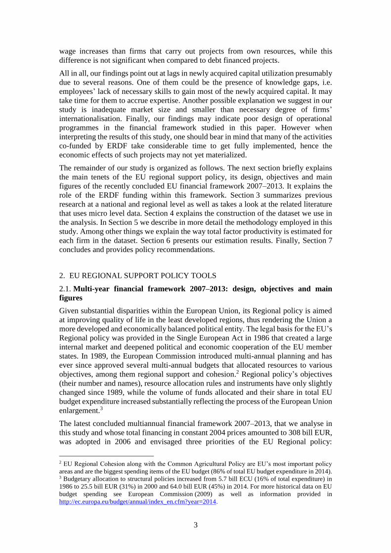
Figure 1. Allocation of the 2007–2013 programming period’s EU funding in Latvia

a. by economic sectors b. by geographical areas

Source: www.esfondi.lv.

6 http://ec.europa.eu/eurostat/tgm/table.do?tab=table&plugin=1&language=en&pcode=tec00114. 7 This figure does not account for funding available from European Agricultural Fund for Rural

Developments (EAFRD) and the European Maritime and Fisheries Fund (EMFF) which are EU Regional

support instruments in Agriculture and Fishing respectively.

Transport

Environment

Entrepreneurship and

innovationEducation

Employment and social

inclusionUrban environment

Science

Health care

Communication

technologiesEnergy

Culture

Other

Riga

All Latvia

Kurzeme

Riga region

Latgale

Zemgale

Vidzeme

6

The composition of the EU funding in Latvia by activity areas and regions is

summarized in Figure 1. Around quarter of all projects are implemented in the field of

Transport, followed by Environment (15%), Entrepreneurship and innovation (12%),

and Education (11%). Looking at the regional dimension of the EU supported projects

around third of them are carried out in Riga or Riga district. Therefore, there is clear

evidence of regional aspect, as each part of Latvia gets its share of the pie (roughly in

accordance to the share in total population).

3. ASSESSING EFFECTIVENESS OF EU REGIONAL POLICY: REVIEW OF

STUDIES

The convergence effect of the EU regional support has been extensively examined in a

number of econometric studies using aggregated national or regional level data (see

Hagen and Mohl, 2011 for a survey). The results of this body of literature has thus far

been rather mixed as the positive effect of the EU funding on national/regional growth

appears to be far from certain. However, while these studies differ with respect to the

choice of the sample, time period, econometric approach and other parameters, some

of them find evidence of a positive effect of the EU support on regional convergence

provided the presence of strong institutions in a recipient region/country that increase

the quality of planning and implementation of projects (e.g. Ederveen et al., 2006;

Gruševaja and Pusch, 2011), high openness of the economy (Ederveen et al., 2003) and

higher degree of decentralisation (Bahr, 2008). The growth effect of the EU funds has

also been shown to be larger when spending is more evenly spread across different

items (Becker et al., 2016), but appears to have been lower during the period of the

Great Recession (Bachtrögler, 2016), i.e. over the programming period 2007–2013 we

consider in our paper.

The impact of the EU funding on firm performance has not been thoroughly

investigated yet, probably due to a lack of detailed firm level data. Yet, those few

studies that evaluate EU policy intervention effects apply a non-experimental setting to

assess the impact of participation on firms’ mean output, employment or/and

productivity. They follow standard microeconometric methods usually employed in

impact evaluation of participation in various national or regional support programmes:

active labour market policies (see e.g. Lechner, 2001), financial support of local

enterprises (Bia and Mattei, 2012), tax credits (Bozio et al., 2014), environmental public

policies (List et al., 2003), and other public interventions. Thus, Pufahl and

Wess (2009) reveal a positive effect of enrolment in EU farm programs on individual

farm sales in Germany. However, the authors do not find any evidence of the positive

effect on farm productivity. The EU support of R&D is shown by Arce and San

Martin (2016) to have a positive effect on Spanish companies’ internal investments in

R&D and employment. As regards the effect of the EU regional policy on regional firm

performance de Zwaan and Merlevede (2014) consider firm level data for

manufacturing firms in all EU member states in 2000–2006. They show that the EU

regional support has no impact on employment or productivity. However, the authors

do not have data on the recipient status of firms and hence employ a two-tiered

matching procedure. They use the propensity score approach to match regions that

receive EU funding with those that do not, and then firms in a former group of regions

are compared with those that are registered in the latter group. The recent paper by

Bachtrögler et al. (2017) is the first one to consider the EU-wide dataset of over two

million individual projects co-financed by the EU regional funds in the programming

7

period 2007–2013. Using this rich dataset and combining it with business data from

ORBIS database they provide an econometric analysis of the determinants of project

values. Largest individual projects are found to be those that a) are co-funded by the

ERDF, b) fall within Convergence objective, c) are transport-related activities, d) are

implemented by very large companies (as classified by ORBIS).

Thus, to the best of our knowledge this study is the first one to assess the effectiveness

of the EU Regional policy, in particular ERDF funding, in fostering productivity and

competitiveness of firms in less developed regions.

4. DATA

4.1. EU funds dataset

For the purpose of the study, we combine several firm-level datasets. The key ingredient

of our empirical analysis is a detailed anonymized dataset of entities8 receiving EU

funding from the ERDF, ESF and the Cohesion Fund, provided by the Ministry of

Finance. This dataset holds information on the amounts received, starting date and end

date, economic sector and location of projects as well as the degree of projects’ risk.

The dataset covers the EU programming period 2007–2013. However, the first year

when entities start making use of the funds available in this period is year 2009 since

the committed funds of the previous programming period 2004–2006 can still be used

up until 2008. Similarly, due to the presence of this N+2 rule, in 2014, the end year of

our dataset, entities continue undertaking activities and receiving funding related to the

2007–2013 period. Overall, we have 2165 entities obtaining regional support from

ERDF, 534 – from ESF and 205 from the Cohesion Fund. As one entity may be

involved in several projects, the total number of projects included in the dataset is

larger, 6493.

As the purposes of these funds differ so does the average project size (in terms of

funding received) and the average length of a project. By far the longest and largest

projects are those financed by the Cohesion fund as these are mainly activities related

to improvements in large transportation networks. Relatively smaller activities are

those co-funded by ERDF as this instrument was designed to aim at raising

competitiveness of small and medium enterprises.

Ultimately, around half of entities had to be dropped from the analysis. First, we had to

exclude the ESF and the Cohesion Fund co-financed activities as most of them are

projects executed by state institutions (Employment Agency, Local Government etc.)

and their inclusion does not comply with the purpose of this study. Many ERDF

beneficiaries are also public sector institutions and hence are also excluded. Second,

there are cases where we lack some of firm performance indicators we analyse, hence

such firms are also excluded. Thus, we end up with ERDF co-financed projects carried

out by 994 companies. In fact, however, the number of firms used in the empirical

analysis is even smaller, as the subsequent performance of those companies that started

receiving ERDF funding in 2013 or later is not yet observed and the sample is restricted

to years until 2013. Furthermore, outlying observations are automatically excluded

from the empirical analysis.

Two thirds of the firms we consider in our analysis fall into the operational programme

Entrepreneurship and Innovation with the activity – Entrepreneurship support –

8 These are enterprises, state agencies, local governments and other legal entities.

8

constituting around 60% of all such companies. Most of the entrepreneurship support

takes the form of the promotion of firms in the foreign markets or aims at facilitating

the developments of micro, small and medium enterprises in lagging regions. 13% of

companies we consider in the study receive financial support for investments with high

value added and innovation related activities. The rest one third of firms under

consideration implement projects classified under the operational programme

Infrastructure and services, largely investments in human capital as well as

environmental projects. Even though this operational programme is the biggest one in

terms of total financing available, the bulk of it is provided from the Cohesion fund and

implemented by public institutions that are out of scope of this study.9

4.2. Latvia’s firm-level database

To perform the analysis of the EU support effectiveness, we need a counterfactual

comprising non-beneficiaries of the EU programmes and a set of impact variables for

both groups of firms. To this end, we make use of few other anonymized firm-level

datasets, provided by the Central Statistical Bureau of Latvia (CSB) and Latvijas

Banka, that contain a myriad of firm specific characteristics for a representative sample

of Latvian commercial enterprises in most areas of activities.10 These datasets are

described in Appendix. Combining all these datasets together, we obtain a large firm-

level database that contains information for the period 2006–2014, with the number of

firms varying between 61’159 in 2006 and 99’466 in 2014.

Table 1 below shows that comparing with population aggregates from Structural

Business Statistics (published by CSB) the firm-level dataset at hand provides a very

high coverage of Latvian enterprises in terms of their number, value added or

employment. The coverage remains high even for small firms.

Table 1. Distribution of firms by size according to Structural Business Statistics and firm-level

dataset in 2014 (B-N, S95, excluding K)

Size

classes

(number of

employees)

Number of firms Value added (th. EUR) Number of employees

Structural

business

statistics

Firm-

level

dataset

Coverage,

%

Structural

business

statistics

Firm-

level

dataset

Coverage,

%

Structural

business

statistics

Firm-

level

dataset

Coverage,

%

0–9 91085 72236 79.3 2056.2 1981.4 96.4 198.0 194.4 98.2

10–19 4739 3360 70.9 833.8 701.3 84.1 63.3 45.1 71.3

20–49 2979 2502 84.0 1432.3 1348.0 94.1 89.1 75.6 84.8

50–249 1486 1551 104.4 2798.2 2947.8 105.3 140.6 150.0 106.6

250–… 202 263 130.2 2966.1 3286.1 110.8 128.7 166.5 129.4

Total 100491 98506 98.0 10086.7 10412.0 103.2 619.7 631.6 101.9 Source: CSB, Latvijas Banka, authors’ calculations.

Notes: The sum of variables for 5 size classes does not correspond to the number in the last row due to missing data on number of

employees for some firms.

We eliminate outlying observations following Lopez-Garzia et al. (2015), who apply a

multi-step exclusion procedure based on the values of various ratios (capital, turnover,

9 Few of these projects are very big infrastructure projects and each of them alone amount to more than

100 mill EUR. 10 We excluded firms from agriculture, forestry and fishing (A), financial and insurance activities (K),

public administration and defence (O), education (P), health (Q), arts, entertainment and recreation (R),

and other services activities (S, except S95, repair of computers and personal and household goods) due

to the lack of data or specific nature of the sector.

9

labour costs, intermediate inputs and value added to labour or capital) and their

numerator and the denominator.11 By that we remove slightly more than 2% of

observations for value added, turnover, capital and wage, while only less than 1% of

observations were removed for the number of employees or intermediate inputs. More

important data losses come from non-reporting of several variables (e.g. number of

employees or size of fixed assets), a problem that is more pronounced for small

enterprises. All in all, after excluding the outliers and accounting for missing values,

we end up with data on 25–30 thousand firms annually.

Finally, several variables were deflated to obtain real values: we deflate value added

and intermediate inputs by industry-specific value added and intermediate inputs

deflators reported by the CSB. Capital stock is deflated by investments deflator.

5. METHODOLOGY

5.1. Propensity score matching approach

For the purpose of this study and in line with other related literature on the effects of

participation in various public intervention programs, we employ a non-experimental

matching technique.

We let the term eui,t∈{0,1} to indicate whether a firm i (treated firm) starts an ERDF

co-financed project in year t; the variable ∆Y1i,t+s to denote the growth rate of a

performance indicator (e.g. change in productivity) of a treated firm at time t+s;12 while

∆Y0i,t+s to define the hypothetical growth rate of a performance indicator of the same

firm, had it not participated in the ERDF co-financed project. Following Heckman et

al. (1997), the average casual effect following the involvement into the ERDF co-

funded project can be represented as:

𝐸[∆𝑌𝑖,𝑡+𝑠1 − ∆𝑌𝑖,𝑡+𝑠

0 |𝑒𝑢𝑖,𝑡 = 1] = 𝐸[∆𝑌𝑖,𝑡+𝑠1 |𝑒𝑢𝑖,𝑡 = 1] − 𝐸[∆𝑌𝑖,𝑡+𝑠

0 |𝑒𝑢𝑖,𝑡 = 1]. (1)

Obviously, the counterfactual outcome ∆Y0i,t+s is unobservable (second term in (1)). To

construct a reliable counterfactual we rely on the performance of those firms (non-

treated or control firms) that do not receive ERDF funding, i.e. 𝐸[∆𝑌𝑖,𝑡+𝑠0 |𝑒𝑢𝑖,𝑡 = 0].

These firms can serve as an appropriate counterfactual if treated firms and firms that do

not participate in ERDF co-funded projects have very similar initial characteristics. In

such a case, we can expect that the selection bias gets insignificant.

In order to approximate the counterfactual 𝐸[∆𝑌𝑖,𝑡+𝑠0 |𝑒𝑢𝑖,𝑡 = 0] accurately, one can

employ matching technique: pairing each treated firm (receiving EU support) with a

similar firm from a valid control group on the basis of some observable characteristics.

Hence the idea is to select such non-treated firms that exhibit the distribution of factors

as similar as possible to those of treated companies. To remove the selection bias, the

set of such factors should include all possible determinants of participation in an ERDF

co-financed project (initial productivity, size, age, experience in EU funds absorption,

exporting status etc.).

11 First, the given ratio is replaced by a missing in case of an abnormal growth – more than two

interquartile ranges above or below the median growth in a respective sector and year. Moreover, the

procedure identifies the source of the extreme growth (numerator or denominator) and replaces it with a

missing. Second, the variable is replaced with a missing if it’s ratio with respect labour or capital falls

into top 1 and 99 percentile of the distribution for the respective ratio. 12 s≥0, so that we analyse the performance after launching an EU supported project.

10

In this study, we employ the propensity score matching approach (PSM, see

Rosenbaum and Rubin, 1983). Matching is performed based on a single index that

measures the probability of a firm to start an ERDF co-funded project conditional upon

initial characteristics of a firm. To identify this probability a probit model of the

following form is estimated:

𝑃𝑟[𝑒𝑢𝑖,𝑡 = 1] = Φ[𝑋𝑖,𝑡−1, 𝑆𝑒𝑐𝑖, 𝑌𝑒𝑎𝑟𝑡], (2)

where Xi,t–1 denotes the set of initial characteristics (in the prior period t–1 to ensure

exogeneity). Some of nonlinear terms and interactions are also included to avoid

inappropriate constraints on the functional form of Φ, alongside a set of dummies to

control for a sector in which a firm operates (Seci, defined at the 2-digit NACE level)

and a year (Yeart).

We denote an estimated probability of starting an ERDF co-financed project for a firm

i at time t in sector k as Pi,k,t. A control firm j with closest propensity score (i.e. closest

predicted probability) is selected as a match for a treated firm. Thus we ensure that

firms have similar characteristics before obtaining ERDF funding and are comparable

We employ the nearest-neighbour matching method both with and without a caliper

that requires a control firm j to be chosen within a certain probability distance:

𝜆 > |𝑃𝑖,𝑘,𝑡 − 𝑃𝑗,𝑘,𝑡| = min𝑗∈{𝑒𝑢𝑗,𝑘,𝑡=0}

(|𝑃𝑖,𝑘,𝑡 − 𝑃𝑗,𝑘,𝑡|). (3)

where λ is a caliper, i.e. a pre-specified scalar that determines maximum allowed

difference in predicted propensity score. If there is no firm found in λ proximity to the

treated firm, then the treated firm is excluded from further analysis. Matching occurs

only within a specified year and NACE sector to ensure comparability of variables

between firms. Alongside one nearest-neighbour matching, we also use two and five

nearest-neighbour matching technique and search for two and five control firms

(accordingly) with the closest propensity score.

Having selected the control group (C) of non-treated matched firms that are similar to

the EU support receiving treated firms (T), we adopt the standard difference-in-

difference (DiD) methodology. It follows the two-step procedure. First, the growth rate

in a firm performance indicator is calculated with respect to the pre-entry year for both

treated and non-treated firms. Then, the means of growth rates are compared and

statistical significance of their differences is estimated:

𝛿𝐷𝑖𝐷,𝑠 =1

𝑁𝑇∑ (∆𝑌𝑖,𝑡+𝑠 − ∑ 𝑤𝑖𝑗∆𝑌𝑗,𝑡+𝑠𝑗,𝑡∈𝐶 )𝑖,𝑡∈𝑇 , 𝑠 ∈ {0,1,2}, (4)

where 𝛿𝐷𝑖𝐷,𝑠 represents the DiD estimator s years following project launch, NT denotes

the number of treated firms, but wij are the weights of controls generated by the

matching algorithm.

The effects of ERDF co-financed project implementation on firm performance may

vary depending on initial characteristics of a firm (productivity and size prior to

participation), or parameters of a project (amount of funds received, degree of project’s

risk, region where a project is undertaken etc.). To gauge the heterogeneous effects on

firm performance we estimate the following equation stating the DiD estimator s years

after the start of a project as a function of pre-treatment characteristics and project

parameters:

(𝑌𝑖,𝑡+𝑠 − ∑ 𝑤𝑖𝑗𝑌𝑗,𝜏+𝑠𝑗,𝜏∈𝐶 ) = 𝛼𝑜 + 𝛼1𝐹𝑖 + 𝛼2𝑍𝑖 + 𝛼3𝑀𝑎𝑐𝑠𝑒𝑐𝑖 + 𝛼4𝑌𝑒𝑎𝑟𝑖 + 𝑒𝑖,𝑡, (6)

11

where Fi denotes firm characteristics, Zi – project parameters.We control for a broad

macroeconomic sector (Macseci)13 in which a firm operates and a year when it launches

a project (Yeari).

As mentioned above, one firm can participate in several ERDF co-funded projects. But

we cannot distinguish between the effect of each individual project, as projects may

overlap. Thus, we are interested in the effect of receiving EU support per se and add

together all projects for each individual firm. Dummy variable eui,t = 1 when a firm

launches it's first ERDF co-funded project during the multiannual financial framework

2007–2013.14 For example, if the first project starts in June 2009, eui,2009 = 1, and we

analyse the performance of the firm in 2009, 2010 and 2011, comparing with the control

firm that was matched based on the performance in 2008.15

5.2. Total factor productivity estimates

Not all of firm performance variables are observable and are part of the dataset. In

particular, we are interested in the effect of participation in ERDF co-funded projects

on total factor productivity (TFP), which should itself be estimated. Here we follow the

approach by Galuscak and Lizal (2011) who use a more elaborated version of

Wooldridge (2009) methodology. Assuming that the production function is of Cobb-

Douglas form, we estimate its coefficients by running the following pooled IV

regression:

𝑙𝑛𝑉𝐴𝑖,𝑡 = 𝛽0 + 𝛽1𝑙𝑛𝐾𝑖,𝑡 + 𝛽2𝑙𝑛𝐿𝑖,𝑡 + ℎ−1(𝑙𝑛𝐾𝑖,𝑡−1, 𝑙𝑛𝑀𝑖,𝑡−1) + 𝛾𝑌𝑒𝑎𝑟𝑡 + 휀𝑖,𝑡 + 𝑢𝑖,𝑡, (7)

where VAi,t, Ki,t, Mi,t are real value added, real capital and real intermediate inputs

respectively for the firm i, Li,t stands for the number of employees, εi,t is an unexpected

shock to the productivity process (that follows random walk with a drift), while ui,t

represents the iid error term. Function h-1 is approximated with a polynomial of order

three. Since number of employees and TFP are simultaneously determined, while

capital takes time to build up, the log of employees is instrumented by its own lagged

values.

We compute firm-level TFP (TFPi,t) as a residual:

𝑙𝑛𝑇𝐹�̂�𝑖,𝑡 = 𝑙𝑛𝑉𝐴𝑖,𝑡 − �̂�0 − �̂�1𝑙𝑛𝐾𝑖,𝑡 − �̂�2𝑙𝑛𝐿𝑖,𝑡 − 𝛾𝑌𝑒𝑎𝑟𝑡. (8)

Similar to Lopez-Garzia et al. (2015), the estimation is performed at a 2-digit industry

level. However, β and γ coefficients are replaced by estimated values obtained at a

corresponding macro-sector if a sector has less than 25 observations per year.

Estimation results can be found in Table A1 in the Appendix.

13 We classify 2-digit NACE industries into the following eleven broad macroeconomic sectors: (1)

mining and quarrying, (2) manufacturing, (3) energy and water supply, (4) construction, (5) wholesale

and retail trade, (6) transportation and storage, (7) accommodation and food service activities, (8)

information and communication, (9) real estate activities, (10) professional, scientific and technical

activities, (11) administrative and support service activities. 14 We cannot observe whether a firm received EU funding during the previous multiannual financial

framework of 2000–2006 due to the lack of necessary data. However, the amount of such firms is smaller

since Latvia joined the EU only in May 2004. 15 Note that the starting date of the project does not correspond to the first transfer of the EU funds to the

firm, which usually comes later.

12

6. EMPIRICAL RESULTS

6.1. Assessing the impact of participation in ERDF supported activities on firm

performance

6.1.1. Conditional probability of participation

First, we calculate firms’ propensity scores, i.e. conditional probabilities to launch an

ERDF co-funded project. As mentioned above, we accomplish this by estimating a

probit regression where we account for the following factors: firm’s productivity

(measured as value added per employee), firm’s age (number of years since it has been

established), number of employees, capital-to-labour ratio, liquidity ratio (represented

by the cash-to-assets ratio), indebtedness indicator (debt-to-assets ratio), ratio of goods

and services exports to turnover, share of employees (managers) with an experience

working for a firm that carried out ERDF co-funded projects in the past. We also include

square terms of some of these variables. Finally, we control for a year and a sector of

the economy in which a firm operates. To avoid problems associated with reverse

causality all the covariates used are taken with one-period lag.

Prior turning to the results of the empirical estimation we perform a simple comparison

of several firm characteristics between ERDF beneficiaries and non-beneficiaries.

Table A2 in the Appendix shows that on average ERDF beneficiaries are older, employ

a larger number of employees and exhibit higher productivity as compared to a sector

average. Furthermore, it is also evident from visual inspection of kernel density of the

log of labour productivity and the log of TFP of beneficiaries and non-beneficiaries of

the ERDF (see Figure A2) as well as from the results of the Kolmogorov-Smirnov test16

that productivity distributions of participants in ERDF co-funded projects tend to

stochastically dominate those of non-participants. Importantly, there is a much smaller

number of observations in the lower tail of the productivity distribution of beneficiaries.

ERDF beneficiaries also tend to be more oriented towards foreign markets as indicated

by a higher share of exports of both goods and services in their turnover.

Some of these regularities are confirmed by the estimation results of the probit

regression (equation (2)) reported in Table 2. In the first specification that includes all

observations in the dataset, labour productivity appears positive and statistically

significant, implying that more productive firms indeed have a-priori higher probability

to participate in an ERDF co-funded activity. In the second specification, the sample is

restricted to years until 2012 as the subsequent performance (in t+1 and t+2) of those

companies that started receiving ERDF funding in 2013 or later is not observed and

these are therefore automatically excluded from further analysis. In this restricted

sample we still confirm a positive labour productivity effect, but it appears now of a

non-linear nature and is more pronounced for more productive firms.

Being a younger firm (rather than an older – as suggested by merely comparing mean

values in Table A2), having a larger firm size and higher capital-to-labour ratio is

associated with higher participation probability, although the latter effect appears

smaller for companies with very high capital-to-labour ratio. Also, the share of exports

of goods in a firm’s turnover is positively associated with participation, probably

meaning that being a player in the global market allows reaping the benefits of

investments more easily and encourages firms to apply for the EU funding, but also

merely reflecting the fact that exports potential is one of the applicants assessment

criteria. As companies by rule are required to cover a certain share of total costs of an

16 Not reported here, but available upon request.

13

EU co-funded project from their own resources, we expect the coefficient on the

liquidity ratio to be positive and statistically significant. However, this coefficient, even

though positive, is not statistically significant in the second sample probably due to a

short length of the restricted sample period. Similarly, while the coefficients before the

share of employees and managers with prior experience in EU co-financed projects

appear positive, these are not statistically significant at any conventional level in the

restricted sample (perhaps the role of experience appears to be important only at the

end of the sample period). Finally, those companies that are part of multinational groups

that originate in one of the OECD countries do not seem to be particularly interested in

applying for the EU regional support as the coefficient is negative and statistically

insignificant in both samples.

Table 2. Factors affecting the probability to launch an ERDF co-funded project (probit estimates,

2008–2014 for full sample and 2008–2012 for PSM sample)

Variables Full sample PSM sample

(1) (2)

Log of labour productivity 0.049** 0.015

Log of labour productivity square 0.007 0.028***

Age -0.047*** -0.070***

Age square 0.002*** 0.003***

Log of employment 0.289*** 0.380***

Log of employment square -0.003 -0.009

Log of capital to labour ratio 0.069*** 0.100***

Log of capital to labour ratio square -0.012*** -0.024***

Liquidity ratio 0.149* 0.135

Indebtedness ratio -0.000 0.000

Exports of goods to turnover 0.487*** 0.490***

Exports of services to turnover 0.075 -0.120

Owner from OECD countries (dummy) -0.212*** -0.307***

Owner from non-OECD countries (dummy) -0.040 -0.178

Share of employees with EU funds experience 0.429** 0.338

Share of managers with EU funds experience 0.638*** 0.517

Year effect Yes Yes

Sector effect Yes Yes

Number of observations 212’242 57’836

Pseudo R2 0.22 0.25 Source: CSB, Latvijas Banka, authors’ calculations.

Note: The full sample is comprised of all observations in the dataset, the PSM sample is restricted to firms that started to receive

EU funds prior to 2013, since we need to observe their performance for the next 2 years. *(**)[***] denotes significance at

0.1(0.05)[0.01] level.

As already indicated above, some of these results corroborate with the assessment

criteria for participation in ERDF co-funded activities. Thus, companies’ submitted

applications for funding in such activities as Promotion in the foreign markets or

Creation of new products and technologies are assessed based on a firm’s (or industry’s

average) exports intensity.17 Labour productivity, measured as value added per

employee, is one of key ingredients in assessing applicants for participation in activity

High value added investments.18 Employees’ wage level is an evaluation criteria for

participation in the activities Creation of new products and technologies and High value

added investments. Few activities (such as e.g. organization of international

17 https://m.likumi.lv/doc.php?id=194223 (Chapter 47.1), https://likumi.lv/doc.php?id=219070

(Annex 3). 18 https://likumi.lv/doc.php?id=238461#p46&pd=1 (Annex 4).

14

conferences on exports promotion) also require firms to have the turnover level above

a certain threshold.19

6.1.2. Matching using nearest neighbour approach

Propensity scores, computed using the coefficients derived from the probit regression

(using column (2) from Table 2), are key elements to perform matching for each treated

firm. The quality of matching is considered successful if it eliminates pre-treatment

differences (evident in the first column of Table 3) between characteristics of firms that

participate and do not participate in the EU regional support. As mentioned above,

matching is implemented using the nearest neighbour approach by additionally

requiring that all combinations of firms come from the same year and sector of the

economy. Letting the opposite occur may have a distortive effect on the evaluation of

treatment effects given substantial fluctuations in Latvian economic developments

across years and sectors. To ensure robustness of our results we perform matching with

1, 2 and 5 nearest control firms as well as without and with a caliper (with the value of

0.05), i.e. the highest allowed propensity score difference between treated companies

and their matched controls, to get rid of potentially bad matches. Finally, we use only

those observations that comply with the common support condition, that excludes

treated firms with a propensity score lower than the smallest one among control firms

and eliminates control firms whose propensity score exceeds the maximum one of the

treated firms.

Table 3. Quality of matching for various methods

Variables

Difference in means of characteristics of treated and control

companies (%) using various methods of matching

Un

mat

ched

1 n

eare

st

nei

ghb

ou

r

2 n

eare

st

nei

ghb

ou

rs

5 n

eare

st

nei

ghb

ou

rs

1 n

eare

st

nei

ghb

ou

r

wit

h c

alip

er

2 n

eare

st

nei

ghb

ou

rs

wit

h c

alip

er

5 n

eare

st

nei

ghb

ou

rs

wit

h c

alip

er

(1) (2) (3) (4) (5) (6) (7)

Log of labour productivity 39.6*** -4.7 -4.2 -2.5 -5.3 -4.2 -3.6

Log of labour productivity square 38.1*** 0.9 -1.9 0.3 0.4 -1.6 -0.9

Age 19.9*** 0.0 2.5 0.9 -1.5 0.4 -1.6

Age square 22.0*** 0.9 3.3 1.2 -0.9 0.7 -1.5

Log of employment 118.5*** 6.4 9.4 14.0** 3.1 4.4 6.8

Log of employment square 106.6*** 10.5 13.2 19.4** 5.6 5.8 9.4

Log of capital to labour ratio 29.7*** 1.7 0.6 1.8 -0.3 -1.4 -1.2

Log of capital to labour ratio square 7.9 4.5 0.4 0.9 2.6 -1.4 -1.5

Liquidity ratio -6.1 8.8 3.8 0.5 8.9 4.0 0.6

Indebtedness ratio -2.9 0.2 0.0 -0.2 0.2 0.4 -0.2

Exports of goods to turnover 75.3*** 2.4 1.7 4.9 0.1 -2.5 -2.5

Exports of services to turnover 8.8* -13.4 -8.5 -6.2 -13.7 -8.8 -7.0

Owner from OECD countries (dummy) 23.6*** 7.8 5.9 7.0 5.4 2.0 3.3

Owner from non-OECD countries (dummy) 14.8*** 0.0 -5.1 0.0 0.0 -7.3 -2.3

Share of employees with EU funds experience 7.4 4.9 -3.0 -0.1 5.3 -3.0 -0.2

Share of managers with EU funds experience 15.6*** 5.1 4.4 0.6 5.4 4.1 -0.2

Number of treated 390 390 390 380 380 380

Number of control 360 684 1570 351 661 1490 Source: CSB, Latvijas Banka, authors’ calculations.

Notes: *(**)[***] denotes significance at 0.1(0.05)[0.01] level. Caliper set to 0.05 in columns (5)–(7).

19 https://m.likumi.lv/doc.php?id=194223 (Chapter 21).

15

Matching quality is satisfactory for most variables using nearest neighbours matching

technique without a caliper, as differences in means of firm characteristics among

treated and control firms prior to starting a project are statistically insignificant. The

only exception refers to a number of employees when five nearest neighbours are used.

However, setting a propensity caliper solves this problem and improves the quality of

matching at a cost of losing few observations.

6.1.3. Difference-in-difference estimators

We estimate difference-in-difference, by comparing changes in mean values of firm

characteristics in three consecutive years with respect to the year prior to involvement

in the ERDF co-funded projects (thus we compare performance in the periods t, t+1 and

t+2 with respect to t–1 to account for differences in initial values). Table 4 reports DiD

estimators for all six different matching methods.

Table 4. Difference-in-difference estimators (DiD) for various methods of matching

Indicator Period

1 nearest

neighbour

2 nearest

neighbours

5 nearest

neighbours

1 nearest

neighbour

with caliper

2 nearest

neighbours

with caliper

5 nearest

neighbours

with caliper

(1) (2) (3) (4) (5) (6)

Log of TFP

t -0.013 -0.018 -0.017 -0.015 -0.027 -0.026

t+1 0.063 0.060 0.057 0.070 0.059 0.056

t+2 0.199** 0.160** 0.148** 0.202** 0.167* 0.162***

Log of labour

productivity

t 0.005 -0.001 -0.004 0.003 -0.011 -0.015

t+1 0.101 0.089 0.078 0.105 0.082 0.071

t+2 0.244*** 0.198** 0.183*** 0.244** 0.193** 0.180***

Log of average

wage

t 0.005 0.010 0.011 0.005 0.011 0.010

t+1 0.055* 0.076** 0.065*** 0.058 0.080*** 0.065***

t+2 0.063* 0.083** 0.077*** 0.066 0.089*** 0.081***

Log of capital to

labour ratio

t 0.155*** 0.147*** 0.133*** 0.156*** 0.145*** 0.131***

t+1 0.272*** 0.272*** 0.259*** 0.275*** 0.268*** 0.252***

t+2 0.380*** 0.401*** 0.361*** 0.379*** 0.394*** 0.349***

Log of

employment

t 0.058* 0.072*** 0.069*** 0.058* 0.075*** 0.070**

t+1 0.099** 0.123*** 0.118*** 0.098** 0.128*** 0.124***

t+2 0.137*** 0.172*** 0.164*** 0.137*** 0.182*** 0.175***

Log of turnover

t 0.073* 0.080** 0.075*** 0.076** 0.085** 0.075**

t+1 0.161*** 0.181*** 0.158*** 0.167*** 0.187*** 0.159***

t+2 0.242*** 0.261*** 0.242*** 0.245*** 0.272*** 0.249***

Exports to turnover

ratio

t 0.006 0.004 0.002 0.006 0.005 0.005

t+1 0.011 0.008 0.013 0.012 0.009 0.012

t+2 0.014 0.007 0.013 0.016 0.011 0.014 Source: CSB, Latvijas Banka, authors’ calculations.

Notes: *(**)[***] denotes significance at 0.1(0.05)[0.01] level. Caliper set to 0.05 in columns (4)–(6). To find the statistical

significance of DiD estimators we use bootstrap procedure with 250 replications.

From Table 4 it is evident that companies that participate in ERDF co-funded activities

raise their employment and capital (the latter at even higher rate, so that there is an

increase in capital-to-labour ratio). These indicators start growing soon after firms

embark on projects and keep on growing until t+2. Firms participating in ERDF co-

funded projects increase their size (number of employees) by approximately 14–18%

in three years comparing with control group's firms, while their capital-to-labour ratio

increases by 35–40%. Increasing input allows ERDF beneficiaries expanding their

16

output and hence turnover in three years by around 25–27% in comparison to non-

beneficiaries.

However, growing capital-to-labour ratio does not translate into higher TFP and labour

productivity immediately. The estimated effect on TFP and labour productivity is close

to zero in the first period and is positive, but insignificant, in the second period.

Productivity gains appear positive and statistically significant only in the third period

after launching a project. Table 4 indicates that labour productivity of participating

companies grows by 18–24% faster compared to non-participating counterparts. Higher

labour productivity also pushes compensation of employees up as treated firms increase

nominal wage by 5–8% in two years after starting an ERDF co-funded project.

The immediate positive effect on capital endowment without a concomitant rise in

firm’s productivity is prima facie surprising. This is possible only if newly installed

capital is not fully utilized in the first two periods. Low capital utilisation after its

instalment may be a sign of the lack of necessary knowledge and experience of using

the acquired capital. Alternatively, it may also signal that firms lack an access to wider

markets to realize their full potential. To this end the estimation results also suggest that

there is no positive effect on exports-to-turnover ratio, implying that firms do not

expand their involvement in the global market to the extent necessary to fully utilize

new capital despite the fact that several ERDF co-funded activities are explicitly aimed

at exports promotion.

6.1.4. Heterogeneity of the treatment effects

It is conceivable that the estimated effects exhibit heterogenous patterns across firms,

regions and projects. Therefore, in this section we examine whether the above reported

DiD estimates vary with different characteristics of firms and projects. To this end we

run cross-sectional regressions for DiD estimators in period t+2 for seven different firm

performance indicators: TFP, labour productivity, wage level, capital-to-labour ratio,

employment, turnover and exports-to-turnover ratio (see Table 5).

Control variables are divided into three categories. First, initial levels of firm

performance indicators are considered. DiD estimators for both TFP and labour

productivity appear larger for initially less productive and larger firms, i.e. these firms

benefit from participation in ERDF co-funded projects to a larger extent than more

productive and smaller firms. The effect on capital-to-labour ratio is found to be larger

for firms with smaller capital-to-labour ratio, while the effect on employment is higher

for initially more productive and smaller firms. Second, regional aspect is addressed by

including dummies for geographical areas where projects are implemented.

Interestingly, neither of the regional dummies included appears statistically significant

which implies that productivity gains or employment increases are similar across the

country. Finally, the last aspect of heterogeneity considered relates to activity. We

would expect larger heterogeneity of DiD estimates across different ERDF co-funded

activities than the one identified in the regressions. The effect on wages is lower for

projects in the activity Science and innovation, presumable reflecting the requirement

that the granted resources in this activity should not be spent to boost personnel salaries.

What is also somewhat puzzling is the absence of any effect on exports-to-turnover

ratio. We have already shown that launching an ERDF co-funded project does not result

in firms becoming more internationally oriented. However we would expect that this is

merely an average estimate and exporting gains might be more visible in the case of

17

activities explicitly aimed at exporting promotion, such as direct marketing activities in

the global market. Unfortunately, this assumption has not been empirically confirmed.

Table 5. Factors affecting difference-in-difference estimators in the period t+2 (DiD, 2 nearest

neighbours with caliper of 0.05)

Variables

Difference-in-difference estimators (DiD) of:

TFP Labour

productivity Wage

Capital to

labour Employment Turnover

Exports to

turnover

Initial productivity (log of TFP) -0.583*** -0.561*** -0.041 0.105 0.097** -0.097* 0.023

Initial size (log of employment) 0.291*** 0.256*** 0.055 -0.083 -0.134* -0.026 -0.023

Age -0.015 -0.014 -0.011* -0.001 -0.006 -0.011 0.000

Initial capital to labour ratio -0.009 -0.032 -0.018 -0.245*** 0.038 0.055 -0.010

Initial exports-to-turnover ratio 0.240 0.154 -0.059 -0.260 0.203 0.187 -0.111

Risk of the project -0.030 -0.022 -0.001 -0.056 -0.034 0.044 -0.038

Size of the project 0.021 0.016 0.015 0.001 -0.002 0.075 -0.009

Riga -0.411 -0.382 -0.085 0.068 0.221 0.367 0.028

Riga region -0.057 0.060 -0.068 0.231 0.013 0.026 0.048

Kurzeme -0.054 -0.026 -0.107 -0.012 -0.077 0.035 0.050

Latgale 0.354 0.504 -0.001 0.400 -0.065 0.167 0.114

Vidzeme 0.002 -0.079 -0.056 0.009 -0.010 0.142 -0.008

Zemgale -0.082 0.046 -0.049 0.529 -0.173 0.091 0.039

Science and innovation -0.170 -0.010 -0.263* -0.014 -0.110 -0.437 -0.028

Entrepreneurship support 0.139 0.287 0.040 0.138 -0.240 -0.202 0.067

Exporting promotion -0.126 -0.531 -0.065 -1.522 0.131 0.298 0.039

Environment protection 0.109 -0.100 -0.108 -1.262* 0.249 -0.099 0.023

Year effect Yes Yes Yes Yes Yes Yes Yes

Macroeconomic sector effect Yes Yes Yes Yes Yes Yes Yes

Number of observations 362 362 362 362 362 362 362

R2 0.343 0.329 0.113 0.254 0.160 0.132 0.088

Source: CSB, Latvijas Banka, authors’ calculations.

Notes: *(**)[***] denotes significance at 0.1(0.05)[0.01] level. Dependent variables are difference-in-difference estimators in t+2

when matching is performed with 2 nearest neighbours with a caliper = 0.05 (column 5 in Table 4).

6.1.5. Robustness section

Finally we perform two robustness checks of the above DiD estimates. First, we

consider timing of a project launch. When a firm embarks on an ERDF co-funded

project closer to the end of a year, it may not be able to start reaping the benefits until

at least the beginning of the next year. In such a case looking at the outcome in the same

year t when a firm launches a project may be misleading. Therefore we perform an

alternative matching of those ERDF beneficiaries that start a project during the last

three months of a year with non-beneficiaries in the next year and gauge their relative

performance considering the next year as year t. The quality of matching appears

satisfactory, and the results of DiD estimation confirm our baseline estimation results

(see Figure 2 for the effect on TFP and Table A3 in the Appendix for a broader range

of results).

Another robustness check is related to the possibility that for a treated and a control

firm may have similar initial level of productivity they still may have been different in

terms of productivity growth. If a treated firm had experienced a more pronounced

productivity growth in the past and occasionally caught up a control firm in period t–1,

it should not come as a surprise that in the future it’s productivity grows faster with

productivity level eventually outpacing that of a control firm. To account for such a

scenario we search for nearest neighbours that are similar in terms of productivity in

both year t–1 and year t–2 so that at least in year t–1 they experienced similar

18

productivity growth. The DiD estimates suggest that productivity gains become smaller

and their significance weaker, suggesting that our previously identified productivity

gains in the third year may be the result of the selection bias not properly addressed by

the chosen matching procedure (see Figure 2 and Table A4 in the Appendix). The

estimation results of cross-sectional regressions for DiD estimators are broadly in line

with the baseline and therefore are not reported for the sake of brevity.

Figure 2. Comparison of DiD estimators for TFP in period t+2 across different matching strategies

and selections of control firms

Source: CSB, Latvijas Banka, authors’ calculations.

Notes: Light columns represent insignificant estimates (not significant at 0.1 level). The first column refers to the baseline DiD

estimator for TFP in t+2 (“baseline”), the second – to the DiD estimator that analyses performance of firms launching a project during the last 3 months of a year starting from the following, rather than the same, year (“3 months lag”), and the third column –

refers to the DiD estimator that is based on matching that considers both initial level of TFP and its initial growth (“level and

growth”).

6.2. Assessing the impact of investment financing source on firm performance

Despite the no-crowding out requirement for receiving the EU funding, it was shown

by Ederveen et al. (2003) that it still to a certain degree replaces the private one.

Therefore, it is useful to analyse the impact of the EU funding on firm performance in

comparison to private funding. In this subsection, we investigate whether the source of

investments matters for company’s further performance. To the best of our knowledge

it is a first such attempt to compare the effect of both funding sources on firm

performance, though there are some studies comparing the effect of different sources

of spending on R&D and innovation (including the EU support).20

To answer the question posed we made some adjustments to our matching procedure.

More specifically, we ensured that a paired control firm has experienced a similar

increase in capital-to-labour ratio (rough proxy for similar investments) as a treated

firm during the three-year period (comparing t+2 with t–1). Thus, again we look at

20 For example, Czarnitzki and Lopes Bento (2014) look at the effects of national subsidies for

innovation in Germany compared to, or in combination with, the effects of European subsidies on

innovation and R&D intensity. The study finds that EU subsidies have smaller impact on firms’ sales.

19

relative performance of similar companies (ERDF beneficiaries and non-beneficiaries)

where this similarity also involves magnitudes of investments made.

Technically, this is done by modifying nearest-neighbour matching described in

equation (3). Now the control firm j is chosen based on the following criteria:

𝜆 > |𝑃𝑖,𝑘,𝑔,𝑡 − 𝑃𝑗,𝑘,𝑔,𝑡| = min𝑗∈{𝑒𝑢𝑗,𝑘,𝑔,𝑡=0}

(|𝑃𝑖,𝑘,𝑔,𝑡 − 𝑃𝑗,𝑘,𝑔,𝑡|). (9)

where Pi,k,g,t denotes the predicted probability of receiving ERDF funding at time t for

a firm i in sector k and in capital-to-labour growth group g. While the capital-to-labour

ratio growth over three years is a continuous variable, we follow Iacus et al. (2012) and

classify firms into several groups. We apply two strategies here: first, firms are

classified into 5 groups according to the quintiles of the capital-to-labour ratio growth

distribution; second, firms are classified into 10 groups according to the deciles of the

same distribution. Afterwards, the nearest-neighbour matching occurs within a

specified year, NACE sector and capital-to-labour growth group.

Table 6. Quality of matching for various methods

Variables

Difference in means of characteristics of treated and control

companies (%) using various methods of matching

Un

mat

ched

2 n

eare

st

nei

ghb

ou

rs,

5 g

roup

s

2 n

eare

st

nei

ghb

ou

rs,

5 g

roup

s,

cali

per

2 n

eare

st

nei

ghb

ou

rs,

10

gro

up

s

2 n

eare

st

nei

ghb

ou

rs,

10

gro

up

s,

cali

per

(1) (2) (3) (4) (5)

Log of labour productivity 39.6*** 8.8 3.0 11.3 5.5

Log of labour productivity square 38.1*** 12.0* 7.6 13.5* 8.6

Age 19.9*** 2.3 -3.5 3.5 -5.8

Age square 22.0*** 2.6 -3.8 4.3 -5.7

Log of employment 118.5*** 25.9*** 11.6 38.1*** 19.1**

Log of employment square 106.6*** 32.7*** 15.2* 43.1*** 21.3**

Log of capital to labour ratio 29.7*** 11.6* 9.4 12.1* 10.1

Log of capital to labour ratio square 7.9 8.6 4.8 8.6 5.0

Liquidity ratio -6.1 -1.7 0.0 -7.3 -3.5

Indebtedness ratio -2.9 -0.6 -0.7 -0.5 -0.2

Exports of goods to turnover 75.3*** 10.0 -8.8 20.3** -2.7

Exports of services to turnover 8.8* -9.3 -11.6 -1.3 -3.7

Owner from OECD countries (dummy) 23.6*** 8.0 6.0 4.1 -3.1

Owner from non-OECD countries (dummy) 14.8*** 7.2 3.5 10.5 -4.9

Share of employees with EU funds experience 7.4 -2.2 -2.3 2.1 -0.4

Share of managers with EU funds experience 15.6*** 0.6 3.6 5.6 1.3

Growth of capital-to-labour ratio (t+2 over t–1) 39.6*** 2.6 3.5 1.8 2.8

Number of treated 382 339 376 326

Number of control 670 596 668 570 Source: CSB, Latvijas Banka, authors’ calculations.

Notes: *(**)[***] denotes significance at 0.1(0.05)[0.01] level. Caliper set to 0.05 in columns (3), (5).

Table 6 reports quality assessment for this modified matching strategy. It can be

observed, that matching over the same year, sector and capital-to-labour growth rate is

rather restrictive, since the number of available controls is scarce. That is why the

quality of matching is lower compared with Table 3, especially with respect to the

initial number of employees, capital-to-labour ratio and exports. However, using caliper

of 0.05, although reducing the number of observations by around 10%, improves the

quality significantly, especially for the case of 5 groups of capital growth. It is important

that an increase in capital-to-labour ratio over the three years period for treated firms is

20

not statistically significantly different from that for non-participating control firms,21

thus all differences in firms performance should be attributed to the difference between

EU funding and private financing, rather than to the magnitude of undertaken

investments.

DiD estimators displayed in Table 7 show that keeping investment constant, we do not

observe large differences in the impact estimates of ERDF funding versus private

financing. If we compare productivity performance, ERDF co-funded projects result in

a larger increase in labour productivity and TFP in the third year, however this

difference is not statistically significant across all matching strategies.

The only striking feature of the EU Regional support program appears in the effect on

employment: participation in ERDF co-funded projects leads to a significantly larger

increase in the number of employees compared to private funding (by around 20% after

three years). This might be related to the assessment process for participation in ERDF

co-funded activities if firms with a potential to increase labour and turnover have a

preference. There is also limited evidence of a higher increase of the wage rate for

ERDF beneficiaries.

Table 7. Difference-in-difference estimators (DiD) for various methods of matching

Indicator Period

2 nearest

neighbours, 5

groups

2 nearest

neighbours, 5

groups, caliper

2 nearest

neighbours, 10

groups

2 nearest

neighbours, 10

groups, caliper

(1) (2) (3) (4)

Log of TFP

t -0.026 -0.031 -0.033 -0.038

t+1 0.056 0.085 0.050 0.047

t+2 0.157** 0.192** 0.114 0.116

Log of labour

productivity

t -0.051 -0.054 -0.048 -0.042

t+1 0.012 0.039 0.011 0.015

t+2 0.100 0.136 0.078 0.087

Log of average wage

t -0.006 -0.005 0.007 0.010

t+1 0.056* 0.064* 0.044 0.057

t+2 0.072** 0.088** 0.049 0.056

Log of capital to

labour ratio

t 0.005 0.013 0.016 0.024

t+1 0.007 0.029 0.001 0.014

t+2 0.031 0.042 0.021 0.033

Log of employment

t 0.105*** 0.103*** 0.096*** 0.091***

t+1 0.157*** 0.154*** 0.158*** 0.151***

t+2 0.218*** 0.219*** 0.196*** 0.195***

Log of turnover

t 0.085** 0.082** 0.077** 0.072**

t+1 0.179*** 0.187*** 0.150*** 0.136***

t+2 0.255*** 0.261*** 0.195*** 0.178***

Exports to turnover

ratio

t 0.006 0.009 0.012 0.012

t+1 0.011 0.014 0.024* 0.026*

t+2 0.021 0.028* 0.028** 0.034** Source: CSB, Latvijas Banka, authors’ calculations

Notes: *(**)[***] denotes significance at 0.1(0.05)[0.01] level. Caliper set to 0.05 in columns (2), (4). To find the statistical

significance of DiD estimators we use bootstrap procedure with 250 replications.

Private financing of capital acquisition usually comes from two alternative sources:

own resources and loans from credit institutions. Therefore we also estimate the effect

of EU funding vis-à-vis these two sources separately. To capture the case of loans

treated ERDF beneficiaries are matched with those ERDF non-beneficiaries, whose

21 Although it is not reported in Table 3 treated and control firms were significantly different in terms of

capital-to-labour growth before, results are available upon request.

21

capital increase is concomitant to an increase in firm’s stock of long-term debt (over

the same period of time) at the amount of at least 50% of acquired capital value.22 To

compare ERDF beneficiaries with those non-beneficiaries that predominantly cover

acquired capital from own resources, treated firms are matched with those firms whose

capital-to labour ratio increase is comparable but whose indebtedness increase is below

the 50% threshold.

Table 8. Difference-in-difference estimators (DiD) for various sources of capital financing

Indicator Period

ERDF financing vs predominantly

loans

ERDF financing vs

predominantly own resources

(1) (2)

Log of TFP

t 0.027 0.003

t+1 0.043 0.063

t+2 0.124 0.156*

Log of labour productivity

t 0.002 -0.008

t+1 -0.014 0.035

t+2 0.064 0.110

Log of average wage

t -0.000 -0.009

t+1 0.051 0.046

t+2 0.074 0.070**

Log of capital to labour ratio

t 0.044 0.052

t+1 0.069 0.034

t+2 0.083* 0.002

Log of employment

t 0.127*** 0.090***

t+1 0.216*** 0.132***

t+2 0.294*** 0.202***

Log of turnover

t 0.142** 0.090**

t+1 0.239*** 0.158***

t+2 0.315*** 0.240***

Exports to turnover ratio

t 0.020 0.028***

t+1 0.021 0.035**

t+2 0.022 0.039**

Number of treated 276 322

Number of control 411 575 Source: CSB, Latvijas Banka, authors’ calculations.

Notes: *(**)[***] denotes significance at 0.1(0.05)[0.01] level. Caliper set to 0.05, 2 nearest neighbours, 5 groups of capital-to-

labour growth. To find the statistical significance of DiD estimators we use bootstrap procedure with 250 replications.

Table 8 shows the DiD estimation results for the case when firms are classified into 5

groups according to the quintiles of the capital-to-labour ratio growth distribution and

a caliper is set at 0.05, as this matching strategy entails better quality.23 No any

remarkable differences between these two cases are uncovered, apart from the fact that

the impact on the increase of exports-to-turnover ratio appears to be statistically

significant when investments are financed by ERDF rather than own resources. There

is also an evidence (although with a weak significance) of productivity and wage

improvements in this case.

7. CONCLUSIONS

This paper examines the casual effect of participating in EU co-funded projects on firm

performance using rich dataset of Latvian firms. The analysis considers ERDF

22 We do not know for sure whether a firm took a loan to finance capital acquisition or for any other

purpose. We make this assumption as the data on the source of investment financing are not available. 23 Results are available upon request.

22

beneficiaries as this EU regional policy instrument is particularly fit to enhance

competitiveness of private companies and therefore is in line with the goal of this paper.

To evaluate the impact of participation in the ERDF co-funded projects we employ

propensity score matching approach, which is widely used in microeconometric

research on the outcome of participation in various publicly sponsored programs. We

find that participation in ERDF co-funded activities raises firm’s capital-to-labour ratio

and employment soon after the start of a project, while a positive effect on labour

productivity takes a longer time to kick in. We also find that there is no statistically

significant productivity premia associated with private versus public (ERDF) financing

of investment projects, though in the latter case firms tend to increase the number of

their employees more rapidly, presumably reflecting selection criteria for participation

in ERDF co-funded projects. Finally, we show that the positive effect on TFP and

labour productivity is more likely to materialize for companies that are bigger and less

productive prior to participation in the EU supported programmes, while the effect on

employment is larger for more productive and relatively smaller firms.

The immediate positive effect on capital endowment without a concomitant rise in

firm’s productivity is surprising. This is possible only if newly installed equipment or

facilities are not fully utilized in the first two periods. Lags in acquired capital

utilization may point at the presence of knowledge gaps, i.e. employees’ lack of

necessary skills to gain most from the installed capital. Alternatively, to attain the EU

funding productivity premium, firms may need to considerably expand their production

by spreading their sales outside the domestic market, which may not happen

immediately.

When interpreting these results one should bear in mind that we consider a participation

moment to occur in the year when a firm starts a project. However, in the case of long

lasting projects taking years, firms may indeed be unable to reap their benefits until

completion. As the end year of our dataset is 2014 we may still be unable to see the full

effect of the financial framework 2007–2013. Moreover, firms that applied for the EU

support in 2013 or 2014 are effectively out of our investigation. In the future,

accumulating longer data series, would allow having more time between launching

ERDF projects and their potential output to draw more precise conclusions regarding

their effectiveness.

On the policy side, we see some room for improvements in the effectiveness of design

and allocation of the EU funds depending on objectives pursued by policymakers. If

the objective is to add more jobs and capital, authorities should presumably target more

productive firms. However, it was shown that such firms might gain relatively less in

terms of subsequent productivity performance. Policy activities that promote

companies internationally would contribute to raising capital utilisation and therefore

allow companies to benefit more from newly installed capital co-funded by the EU. To

this end, the fact that participation in external promotion activities yields similar impact

on subsequent exporting as participation in other ERDF co-funded programmes, where

explicit promotion of exports is not considered as the main objective, is striking and

might indicate that such activities should be better designed.

Since a positive effect on employment appears as a highly robust finding across various

matching strategies, it would be interesting in future researches to analyse the origins

of extra labour attracted. If labour comes from a pool of unemployed or inactive

persons, ERDF projects improve national employment figures. However, if new

23

employees come from other enterprises, ERDF may have an adverse effect on

allocation of labour.

24

References

Arce Ignacio, San Martin Milagros (2016) An Impact Evaluation of the EU Funds on Research

and Development in Spanish Companies in 2007-2011. Instituto de Estudios Fiscales.

Bachtrögler Julia (2016) On the Effectiveness of the EU Structural Funds during the Great

Recession: Estimates from a Heterogeneous Local Average Treatment Effects Framework.

Department of Economics Working Paper Series 230. WU Vienna University of Economics

and Business.

Bachtrögler Julia, Hammer Christoph, Reuter Wolf Heinrich, Schwendinger Florian (2017)

Spotlight on the Beneficiaries of EU Regional Funds: A New Firm-level Dataset. Department

of Economics Working Paper Series 246. WU Vienna University of Economics and Business.

Bahr Cornelius (2008) How Does Sub-National Autonomy Affect the Effectiveness of

Structural Funds? Kyklos, 61(1), pp. 3–18.

Becker Sascha, Egger Peter, von Ehrlich Maximilian (2016) Effects of EU Regional Policy:

1989 – 2013. The University of Warwick, Working Paper Series No. 271.

Bia Michela, Mattei Alessandra (2012) Assessing the Effect of the Amount of Financial Aids

to Piedmont Firms Using the Generalized Propensity Score. Statistical Methods and

Applications 21(4), pp. 485–516.

Bozio Antoine, Irac Delphine, Py loriane (2014) Impact of Research Tax Credit on R&D and

Innovation: Evidence from the 2008 French Reform. Bank of France Working Paper No. 532.

Czarnitzki and Lopes Bento (2014) Innovation Subsidies: Does the Funding Source Matter for

Innovation Intensity and Performance? Empirical Evidence from Germany. Industry and

Innovation, 21(5). pp. 380–409.

De Loecker, J. (2013) Detecting Learning by Exporting. American Economic Journal:

Microeconomics, 5(3), pp. 1–21.

Ederveen Sjed, Gorter Joeri, de Mooji Ruud, Nahuis Richard (2003) Funds and Games: The

Economics of European Cohesion Policy. European Network of Economic Policy Research

Institutes, Occasional paper No. 3.

Ederveen Sjed, de Groot Joeri, Nahuis Richard (2006) Fertile Soil for Structural Funds? A Panel

Data Analysis of the Conditional Effectiveness of European Cohesion Policy. Kyklos, 59,

pp. 17–42.

European Commission (2007) Cohesion policy 2007–2013: Commentaries and Official Texts

http://ec.europa.eu/regional_policy/sources/docoffic/official/regulation/pdf/2007/publications/

guide2007_en.pdf.

European Commission (2009) EU Budget 2008 Financial Report

http://ec.europa.eu/budget/library/biblio/publications/2008/fin_report/fin_report_08_en.pdf.

European Commission (2014) The European Union Explained: Regional Policy, 2014.

European Council (2006) Council Decision of 6 October 2006 on Community Strategic

Guidelines on Cohesion. 2006/702/EC http://eur-

lex.europa.eu/LexUriServ/LexUriServ.do?uri=OJ:L:2006:291:0011:0032:EN:PDF.

Galuscak Kamil, Lizal Lubomir (2011) The Impact of Capital Measurement Error Correction

on Firm-Level Production Function Estimation. Czech National Bank Working Paper No.

9/2011.

Gruševaja Marina, Pusch Toralf (2011) How Does Institutional Setting Affect the Impact of EU

Structural Funds on Economic Cohesion? New Evidence from Central and Eastern Europe.

IWH Discussion paper, No. 17.

25

Hagen Tobias, Mohl Philipp (2011) Econometric Evaluation of EU Cohesion Policy: A Survey.

In: International Handbook on the Economics of Integration, Volume III, chapter 16 Edward

Elgar Publishing.

Heckman Elhanan, Melitz Marc, Yeaple Stephen (2004) Export versus FDI with Heterogenous

Firms. American Economic Review, 94(1), pp. 300–316.

Iacus, S.M., King, G., and Porro, G. (2012) Causal Inference without Balance Checking:

Coarsened Exact Matching. Political Analysis, 20(1), pp. 1–24.

Lechner Michael (2001) Program Heterogeneity and propensity Score Matching: An

Application to the Evaluation of Active Labour Market Policies. The Review of Economics and

Statistics, 84(2), pp. 205–220.

List John, Millimet Daniel, Fredriksson Per, McHone Warren (2003) Effects of Environmental

Regulations on Manufacturing Plant Births: Evidence from a Propensity Score Matching

Estimator. The Review of Economics and Statistics, 85(4), pp. 944–952.

Lopez-Garcia Paloma, di Mauro Filippo and the CompNet Task Force (2015) Assessing

European Competitiveness: The New CompNet Microbased Database. ECB Working Paper

No. 1764.

Pufahl Andrea, Weiss Christoph (2009) Evaluating the Effects of Farm Programmes: Results

from Propensity Score Matching. European Review of Agricultural Economics, 36(1), pp. 79–

101.

Rosenbaum Paul, Rubin Donald (1983) The Central Role of the Propensity Score in

Observational Studies for Casual Effects. Biometrika, 70(1), pp. 41–55.

Wooldridge Jeffrey (2009) On Estimating Firm-Level Production Functions using Proxy

Variables to Control for Unobservables. Economics Letters, 104(3), pp. 112–114.

de Zwaan Matthijs, Merlevede Bruno (2014) Regional Policy and Firm Productivity, European

Trade Study Group Working paper, No. 377.

26

Appendix

Firm-level datasets used in the study

In this study, apart from the dataset containing information on EU co-financed projects,

the following firm-level datasets are used:

Firms’ indicators comprehensive database that contains records from companies’

balance sheets and profit and loss statements as well as provides data on value added,

number of employees, personnel costs, production value and the use of intermediate

inputs. Data are collected on the basis of CSB annual statistical report “1-annual”,

“Complex report on activities” and reports to the State Revenue Service.

Goods external trade database that includes data on merchandise flows (exports and

imports) where merchandise is classified according to the eight-digit Combined

Nomenclature (CN8) classification. This database is based on data coming from two

sources: INTRASTAT surveys for Latvia’s trade with other EU member states and

custom declarations for trade with countries outside the EU.

Services external trade database, collected by Latvijas Banka, provides data on export

and import flows for all types of services apart from travel, construction, insurance and

government services for which detailed firm-level information is not collected and other

sources are used for the balance of payments purpose.

Firms’ foreign assets and liabilities dataset, also collected by Latvijas Banka, provides

information on external assets and liabilities of firms. This dataset allows detecting

companies with direct foreign owners (including the country of origin of an owner).

Employer-employee data, provided by CSB and based on the State Revenue Service

information from companies’ social insurance tax declarations allows to track

employees with an experience working on projects co-funded by the EU regional

support instruments.

Table A1. Coefficients of the Cobb-Douglas production function

Sector Coefficient

before labour

(�̂�1)

Coefficient

before capital

(�̂�2)

Number of

observations

05 Mining of coal and lignite 0.669*** 0.302*** 718†

06 Extraction of crude petroleum 0.669*** 0.302*** 718†

07 Mining of metal ores 0.669*** 0.302*** 718†

08 Other mining and quarrying 0.668*** 0.302*** 711

09 Mining support service activities 0.669*** 0.302*** 718†

10 Manufacture of food products 0.611*** 0.183*** 2814

11 Manufacture of beverages 0.743*** 0.392*** 267

12 Manufacture of tobacco products 0.681*** 0.197*** 24406†

13 Manufacture of textiles 0.658*** 0.172*** 639

14 Manufacture of wearing apparel 0.894*** 0.162*** 1584

15 Manufacture of leather and related products 1.044*** 0.129** 190

16 Manufacture of wood and products of wood and cork 0.502*** 0.257*** 4335

17 Manufacture of paper and paper products 0.638*** 0.162** 389

18 Printing of reproduction of recorded media 0.785*** 0.200*** 1581

19 Manufacture of coke and refined petroleum products 0.681*** 0.197*** 24406†

20 Manufacture of chemicals and chemical products 0.629*** 0.192*** 656

21 Manufacture of basic pharmaceutical products 0.681*** 0.197*** 24406†

22 Manufacture of rubber and plastic products 0.843*** 0.171*** 975

23 Manufacture of other non-metallic mineral products 0.519*** 0.157*** 1242

24 Manufacture of basic metals 0.681*** 0.197*** 24406†

27

25 Manufacture of fabricated metal products 0.729*** 0.207*** 2796

26 Manufacture of computer, electronic and optical products 0.719*** 0.182*** 474

27 Manufacture of electrical equipment 0.824*** 0.177*** 329

28 Manufacture of machinery and equipment n.e.c. 0.629*** 0.238*** 680

29 Manufacture of motor vehicles, trailers and semi-trailers 0.681*** 0.197*** 24406†

30 Manufacture of other transport equipment 0.681*** 0.197*** 24406†

31 Manufacture of furniture 0.633*** 0.205*** 2011

32 Other manufacturing 0.861*** 0.155*** 880

33 Repair and installation of machinery and equipment 0.774*** 0.180*** 2005

35 Electricity, gas, steam and air conditioning supply 0.284*** 0.109** 1503

36 Water collection, treatment and supply 0.416*** 0.181*** 2717†

37 Sewerage 0.728*** 0.020 247

38 Waste collection, treatment and disposal activities 0.695*** 0.210*** 727

39 Remediation activities and other waste management services 0.416*** 0.181*** 2717†

41 Construction of buildings 0.543*** 0.170*** 4873

42 Civil engineering 0.705*** 0.247*** 1855

43 Specialised construction activities 0.766*** 0.204*** 10621

45 Wholesale and retail trade and repair of motor vehicles 0.695*** 0.146*** 10455

46 Wholesale trade, except of motor vehicles and motorcycles 0.518*** 0.163*** 28831

47 Retail trade, except of motor vehicles and motorcycles 0.687*** 0.112*** 30926

49 Land transport and transport via pipelines 0.535*** 0.188*** 11809

50 Water transport 0.680*** 0.166*** 18240†

51 Air transport 0.680*** 0.166*** 18240†

52 Warehousing and support activities for transportation 0.773*** 0.157*** 6004

53 Postal and courier activities 0.680*** 0.166*** 18240†

55 Accommodation 0.550*** 0.194*** 2014

56 Food and beverage service activities 0.693*** 0.134*** 5653

58 Publishing activities 0.928*** 0.126*** 1487

59 Video programme production, sound recording and music publishing 0.914*** 0.181*** 665

60 Programming and broadcasting activities 0.916*** 0.201*** 9448†

61 Telecommunications 0.846*** 0.243*** 1320

62 Computer programming, consultancy and related activities 0.972*** 0.188*** 4170

63 Information service activities 0.991*** 0.221*** 1410

68 Real estate activities 0.500*** 0.093*** 16264

69 Legal and accounting activities 0.919*** 0.126*** 10305

70 Activities of head offices; management consultancy activities 0.846*** 0.144*** 3816

71 Architectural and engineering activities 0.859*** 0.201*** 5143

72 Scientific research and development 0.703*** 0.061 377

73 Advertising and market research 0.847*** 0.182*** 4866

74 Other professional, scientific and technical activities 0.736*** 0.195*** 2445

75 Veterinary activities 0.824*** 0.161*** 27344†

77 Rental and leasing activities 0.525*** 0.226*** 2465

78 Employment activities 0.894*** 0.236*** 712

79 Travel agency, tour operator and related activities 0.954*** 0.124*** 1764

80 Security and investigation activities 0.911*** 0.101*** 1214

81 Services to buildings and landscape activities 0.881*** 0.110*** 1845

82 Office administrative, office support and other activities 0.874*** 0.061 770 Source: CSB, Latvijas Banka, authors’ calculations.

Notes: *(**)[***] denotes significance at 0.1(0.05)[0.01] level. † reflects that estimates were made on a broad macroeconomic

sector level.

Table A2. Comparison of ERDF beneficiaries and non-beneficiaries

Firm characteristics ERDF beneficiaries (N = 994)

ERDF non-beneficiaries

(N = 547’470)

Mean Standard deviation Mean Standard deviation

Age 9.04 6.67 7.18 5.91

Number of employees 59.85 167.05 10.64 76.11

Log of relative labour productivity* 0.61 1.12 0.00 1.30

Log of relative TFP* 0.71 1.12 0.00 1.24

Ln of relative capital-to-labour ratio* 0.80 1.88 0.00 2.05

Exporter of goods and/or services (dummy) 0.43 0.50 0.07 0.26

Exports of goods to turnover 0.17 0.29 0.02 0.10

Exports of services to turnover 0.02 0.13 0.01 0.07 * relative to average in sector and year.

28

Figure A1. Distribution of productivity for firms obtaining ERDF funding, comparing with other

firms

a. log of labour productivity b. log of TFP

Source: CSB, Latvijas Banka, authors’ calculations.

Table A3. Difference-in-difference estimators (DiD) for various methods of matching (addressing

the problem of the end of a year)

Indicator Period

1 nearest

neighbour

2 nearest

neighbours

5 nearest

neighbours

1 nearest

neighbour

with caliper

2 nearest

neighbours

with caliper

5 nearest

neighbours

with caliper

(1) (2) (3) (4) (5) (6)

Log of TFP

t -0.033 -0.018 0.014 -0.037 -0.019 0.013

t+1 -0.002 0.043 0.071 0.005 0.051 0.083

t+2 0.164* 0.182** 0.165*** 0.166* 0.201*** 0.193***

Log of labour

productivity

t -0.007 0.001 0.025 -0.014 -0.005 0.019

t+1 0.020 0.073 0.098* 0.018 0.074 0.099

t+2 0.170* 0.211*** 0.197*** 0.166* 0.220*** 0.210***

Log of average

wage

t 0.035 0.034 0.010 0.031 0.030 0.008

t+1 0.091*** 0.091*** 0.063*** 0.088** 0.090*** 0.062**

t+2 0.079** 0.101*** 0.085*** 0.075* 0.102*** 0.088***

Log of capital to

labour ratio

t 0.150*** 0.133*** 0.126*** 0.132** 0.118** 0.106**

t+1 0.216*** 0.238*** 0.258*** 0.192** 0.225*** 0.234***

t+2 0.260*** 0.297*** 0.334*** 0.234*** 0.282*** 0.311***

Log of

employment

t 0.099*** 0.091*** 0.094*** 0.098*** 0.091*** 0.096***

t+1 0.170*** 0.135*** 0.130*** 0.173*** 0.134*** 0.136***

t+2 0.237*** 0.182*** 0.184*** 0.239*** 0.184*** 0.190***

Log of turnover

t 0.085** 0.092*** 0.090*** 0.084** 0.093*** 0.089***

t+1 0.148*** 0.155*** 0.150*** 0.153*** 0.159*** 0.156***

t+2 0.254*** 0.244*** 0.233*** 0.256*** 0.252*** 0.243***

Exports to turnover

ratio

t 0.008 0.017 0.013 0.009 0.018* 0.015*

t+1 0.006 0.018 0.018 0.008 0.019 0.019

t+2 0.002 0.011 0.013 0.004 0.012 0.014 Source: CSB, Latvijas Banka, authors’ calculations. Notes: *(**)[***] denotes significance at 0.1(0.05)[0.01] level. Caliper set to 0.05 in columns (4)–(6). To find the statistical

significance of DiD estimators we use bootstrap procedure with 250 replications.

29

Table A4. Difference-in-difference estimators (DiD) for various methods of matching (matching

with firms having similar labour productivity in both t–1 and t–2)

Indicator Period

1 nearest

neighbour

2 nearest

neighbours

5 nearest

neighbours

1 nearest

neighbour

with caliper

2 nearest

neighbours

with caliper

5 nearest

neighbours

with caliper

(1) (2) (3) (4) (5) (6)

Log of TFP

t 0.029 -0.023 0.005 0.016 -0.035 -0.003

t+1 0.070 0.057 0.062 0.062 0.042 0.047

t+2 0.146* 0.118 0.085 0.137 0.108 0.082

Log of labour

productivity

t 0.039 -0.015 0.020 0.028 -0.026 0.013

t+1 0.101 0.079 0.091 0.092 0.065 0.078

t+2 0.152* 0.139* 0.115* 0.144 0.124 0.108

Log of average

wage

t 0.002 0.010 0.008 0.002 0.010 0.010

t+1 0.066* 0.064** 0.062** 0.062* 0.061** 0.059**

t+2 0.088** 0.088** 0.083*** 0.086** 0.088*** 0.085***

Log of capital to

labour ratio

t 0.128** 0.115*** 0.133*** 0.132*** 0.115** 0.136***

t+1 0.264*** 0.258*** 0.270*** 0.272*** 0.260*** 0.270***

t+2 0.329*** 0.347*** 0.353*** 0.341*** 0.351*** 0.357***

Log of

employment

t 0.074** 0.065*** 0.058*** 0.074** 0.066** 0.057**

t+1 0.141*** 0.122*** 0.110*** 0.140*** 0.127*** 0.115***

t+2 0.229*** 0.181*** 0.160*** 0.229*** 0.195*** 0.169***

Log of turnover

t 0.081** 0.073** 0.071** 0.078* 0.070** 0.064**

t+1 0.172*** 0.159*** 0.145*** 0.168*** 0.151*** 0.135***

t+2 0.269*** 0.234*** 0.212*** 0.265*** 0.231*** 0.203***

Exports to turnover

ratio

t 0.012 0.009 0.006 0.015 0.011 0.010

t+1 0.034** 0.027* 0.018 0.036** 0.029 0.021*

t+2 0.043*** 0.029** 0.023* 0.045** 0.032* 0.025** Source: CSB, Latvijas Banka, authors’ calculations.

Notes: *(**)[***] denotes significance at 0.1(0.05)[0.01] level. Caliper set to 0.05 in columns (4)–(6). To find the statistical

significance of DiD estimators we use bootstrap procedure with 250 replications.