
THE IMPLICIT FUNCTION THEOREM Statement of the … · Statement of the theorem. Theorem 1 ... Given...
24
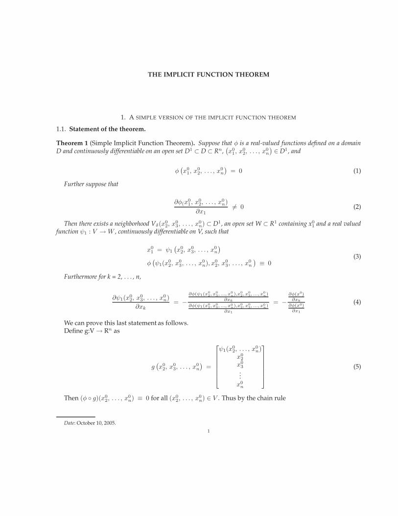
THE IMPLICIT FUNCTION THEOREM 1. A SIMPLE VERSION OF THE IMPLICIT FUNCTION THEOREM 1.1. Statement of the theorem. Theorem 1 (Simple Implicit Function Theorem). Suppose that φ is a real-valued functions defined on a domain D and continuously differentiable on an open set D 1 ⊂ D ⊂ R n , ( x 0 1 ,x 0 2 ,...,x 0 n ) ∈ D 1 , and φ ( x 0 1 ,x 0 2 ,...,x 0 n ) =0 (1) Further suppose that ∂φ ( x 0 1 ,x 0 2 ,...,x 0 n ) ∂x 1 =0 (2) Then there exists a neighborhood V δ (x 0 2 ,x 0 3 ,...,x 0 n ) ⊂ D 1 , an open set W ⊂ R 1 containing x 0 1 and a real valued function ψ 1 : V → W , continuously differentiable on V, such that x 0 1 = ψ 1 ( x 0 2 ,x 0 3 ,...,x 0 n ) φ ( ψ 1 (x 0 2 ,x 0 3 ,...,x 0 n ),x 0 2 ,x 0 3 ,...,x 0 n ) ≡ 0 (3) Furthermore for k = 2, ... , n, ∂ψ 1 (x 0 2 ,x 0 3 ,...,x 0 n ) ∂x k = - ∂φ(ψ1(x 0 2 ,x 0 3 ,...,x 0 n ),x 0 2 ,x 0 3 ,...,x 0 n ) ∂xk ∂φ(ψ1(x 0 2 ,x 0 3 ,...,x 0 n ),x 0 2 ,x 0 3 ,...,x 0 n ) ∂x1 = - ∂φ(x 0 ) ∂xk ∂φ(x 0 ) ∂x1 (4) We can prove this last statement as follows. Define g:V → R n as g ( x 0 2 ,x 0 3 ,...,x 0 n ) = ψ 1 (x 0 2 ,...,x 0 n ) x 0 2 x 0 3 . . . x 0 n (5) Then (φ ◦ g)(x 0 2 ,...,x 0 n ) ≡ 0 for all (x 0 2 ,...,x 0 n ) ∈ V . Thus by the chain rule Date: October 10, 2005. 1
Transcript of THE IMPLICIT FUNCTION THEOREM Statement of the … · Statement of the theorem. Theorem 1 ... Given...
THE IMPLICIT FUNCTION THEOREM
1. A SIMPLE VERSION OF THE IMPLICIT FUNCTION THEOREM
1.1. Statement of the theorem.
Theorem 1 (Simple Implicit Function Theorem). Suppose that φ is a real-valued functions defined on a domainD and continuously differentiable on an open set D1 ⊂ D ⊂ Rn,
(x0
1, x02, . . . , x
0n
)∈ D1, and
φ(x0
1, x02, . . . , x
0n
)= 0 (1)
Further suppose that
∂φ(x01, x
02, . . . , x
0n)
∂x16= 0 (2)
Then there exists a neighborhood Vδ(x02, x
03, . . . , x
0n) ⊂ D1, an open set W ⊂ R1 containing x0
1 and a real valuedfunction ψ1 : V →W , continuously differentiable on V, such that
x01 = ψ1
(x0
2, x03, . . . , x
0n
)
φ(ψ1(x0
2, x03, . . . , x
0n), x
02, x
03, . . . , x
0n
)≡ 0
(3)
Furthermore for k = 2, . . . , n,
∂ψ1(x02, x
03, . . . , x
0n)
∂xk= −
∂φ(ψ1(x02, x
03, ..., x
0n),x0
2, x03, ..., x
0n)
∂xk
∂φ(ψ1(x02, x
03, ..., x
0n),x0
2, x03, ..., x
0n)
∂x1
= −∂φ(x0)∂xk
∂φ(x0)∂x1
(4)
We can prove this last statement as follows.Define g:V → Rn as
g(x0
2, x03, . . . , x
0n
)=
ψ1(x02, . . . , x
0n)
x02
x03...x0n
(5)
Then (φ ◦ g)(x02, . . . , x
0n) ≡ 0 for all (x0
2, . . . , x0n) ∈ V . Thus by the chain rule
Date: October 10, 2005.1
2 THE IMPLICIT FUNCTION THEOREM
D (φ ◦ g)(x02, . . . , x
0n) = Dφ
(g(x0
2, . . . , x0n)
)D g(x0
2, . . . x0n) = 0
= Dφ(x0
1, x02, . . . , x
0n
)D g(x0
2, . . . x0n) = 0
= D φ
x01
x02
x03...x0n
D
ψ1(x02, . . . , x
0n)
x02
x03...x0n
= 0
⇒[∂φ∂x1
, ∂φ∂x2, . . . , ∂φ∂xn
]
∂ψ1∂x2
∂ψ1∂x3
. . . ∂ψ1∂xn
1 0 . . . 00 1 . . . 0...
... . . ....
0 0 . . . 1
=[0 0 . . . 0
]
(6)
For any k = 2, 3, . . . , n, we then have
∂φ(x01, x
02, . . . , x
0n)
∂x1
∂ψ1(x02, . . . , x
0n)
∂xk+
∂φ(x01, x
02, . . . , x
0n)
∂xk= 0
⇒ ∂ψ1(x02, . . . , x
0n)
∂xk= −
∂φ(x01,x
02,...,x
0n)
∂xk
∂φ(x01,x
02,...,x
0n)
∂x1
(7)
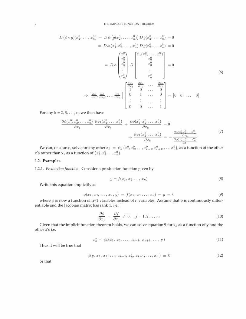
We can, of course, solve for any other xk = ψk(x0
1, x02, . . . , x
0k−1, x
0k+1, . . . , x
0n
), as a function of the other
x’s rather than x1 as a function of(x0
2, x03 . . . , x
0n
).
1.2. Examples.
1.2.1. Production function. Consider a production function given by
y = f(x1, x2 . . . , xn) (8)Write this equation implicitly as
φ(x1, x2, . . . , xn, y) = f(x1, x2 . . . , xn) − y = 0 (9)where φ is now a function of n+1 variables instead of n variables. Assume that φ is continuously differ-
entiable and the Jacobian matrix has rank 1. i.e.,
∂φ
∂xj=
∂f
∂xj6= 0, j = 1, 2, . . . , n (10)
Given that the implicit function theorem holds, we can solve equation 9 for xk as a function of y and theother x’s i.e.
x∗k = ψk(x1, x2, . . . , xk−1, xk+1, . . . , y ) (11)Thus it will be true that
φ(y, x1, x2, . . . , xk−1, x∗k, xk+1, . . . , xn ) ≡ 0 (12)
or that

THE IMPLICIT FUNCTION THEOREM 3
y ≡ f(x1, x2, . . . , xk−1, x∗k, xk+1, . . . , xn ) (13)
Differentiating the identity in equation 13 with respect to xj will give
0 =∂f
∂xj+
∂f
∂xk
∂xk∂xj
(14)
or
∂xk∂xj
=− ∂f
∂xj
∂f∂xk
= RTS = MRS (15)
Or we can obtain this directly as
∂φ(y, x1, x2, . . . , xk−1, ψk, xk+1, . . . , xn)∂xk
∂ψk∂xj
=−∂φ(y, x1, x2, . . . , xk−1, ψk, xk+1, . . . , xn)
∂xj
⇒ ∂φ
∂xk
∂xk∂xj
= − ∂φ
∂xj
⇒ ∂xk∂xj
=− ∂f
∂xj
∂f∂xk
= MRS
(16)
Consider the specific example
y0 = f (x1, x2 ) = x21 − 2x1 x2 + x1 x
32
To find the partial derivative of x2 with respect to x1 we find the two partials of f as follows
∂x2
∂x1= −
∂ f∂x1
∂ f∂x2
= − 2x1 − 2x2 + x32
3x1 x22 − 2x1
=2x2 − 2x1 − x3
2
3x1 x22 − 2x1
1.2.2. Utility function.u0 = u (x1, x2 )
To find the partial derivative of x2 with respect to x1 we find the two partials of U as follows
∂x2
∂x1= −
∂ u∂x1
∂ u∂x2
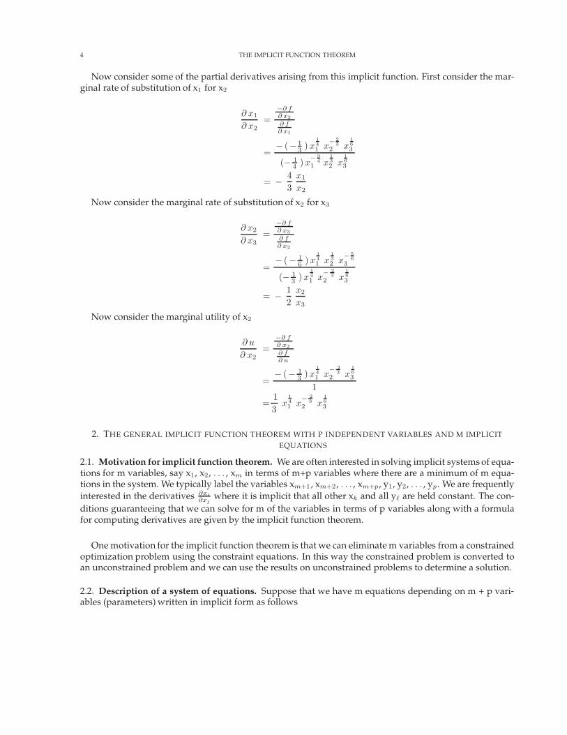
1.2.3. Another utility function. Consider a utility function given by
u = x141 x
132 x
163
This can be written implicitly as
f (u, x1, x2, x3 ) = u − x141 x
132 x
163 = 0
4 THE IMPLICIT FUNCTION THEOREM
Now consider some of the partial derivatives arising from this implicit function. First consider the mar-ginal rate of substitution of x1 for x2
∂ x1
∂ x2=
−∂ f∂ x2
∂ f∂ x1
=− (−1
3)x
141 x
−23
2 x163
(− 14 )x−
34
1 x132 x
163
= − 43x1
x2
Now consider the marginal rate of substitution of x2 for x3
∂ x2
∂ x3=
−∂ f∂ x3
∂ f∂ x2
=− (− 1
6)x
141 x
132 x
− 56
3
(− 13 )x
141 x
− 23
2 x163
= − 12x2
x3
Now consider the marginal utility of x2
∂ u
∂ x2=
−∂ f∂ x2
∂ f∂ u
=− (− 1
3)x
141 x
− 23
2 x163
1
=13x
141 x
− 23
2 x163
2. THE GENERAL IMPLICIT FUNCTION THEOREM WITH P INDEPENDENT VARIABLES AND M IMPLICITEQUATIONS
2.1. Motivation for implicit function theorem. We are often interested in solving implicit systems of equa-tions for m variables, say x1, x2, . . . , xm in terms of m+p variables where there are a minimum of m equa-tions in the system. We typically label the variables xm+1 , xm+2 , . . . , xm+p, y1, y2, . . . , yp. We are frequentlyinterested in the derivatives ∂xi
∂xjwhere it is implicit that all other xk and all y` are held constant. The con-
ditions guaranteeing that we can solve for m of the variables in terms of p variables along with a formulafor computing derivatives are given by the implicit function theorem.
One motivation for the implicit function theorem is that we can eliminate m variables from a constrainedoptimization problem using the constraint equations. In this way the constrained problem is converted toan unconstrained problem and we can use the results on unconstrained problems to determine a solution.
2.2. Description of a system of equations. Suppose that we have m equations depending on m + p vari-ables (parameters) written in implicit form as follows
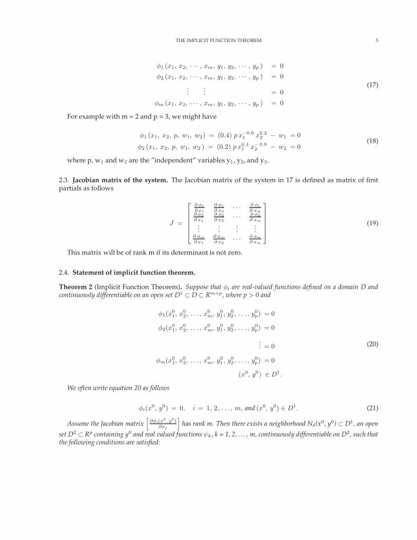
THE IMPLICIT FUNCTION THEOREM 5
φ1 (x1, x2, · · · , xm, y1, y2, · · · , yp ) = 0
φ2 (x1, x2, · · · , xm, y1, y2, · · · , yp ) = 0
...... = 0
φm (x1, x2, · · · , xm, y1, y2, · · · , yp ) = 0
(17)
For example with m = 2 and p = 3, we might have
φ1 (x1, x2, p, w1, w2) = (0.4) p x−0.61 x0.2
2 − w1 = 0
φ2 (x1, x2, p, w1, w2 ) = (0.2) p x0.41 x− 0.8
2 − w2 = 0(18)
where p, w1 and w2 are the ”independent” variables y1, y2, and y3.
2.3. Jacobian matrix of the system. The Jacobian matrix of the system in 17 is defined as matrix of firstpartials as follows
J =
∂ φ1∂ x1
∂ φ1∂ x2
· · · ∂ φ1∂ xm
∂ φ2∂ x1
∂ φ2∂ x2
· · · ∂ φ2∂ xm
......
......
∂ φm
∂ x1
∂ φm
∂ x2· · · ∂ φm
∂ xm
(19)
This matrix will be of rank m if its determinant is not zero.
2.4. Statement of implicit function theorem.
Theorem 2 (Implicit Function Theorem). Suppose that φi are real-valued functions defined on a domain D andcontinuously differentiable on an open set D1 ⊂ D ⊂ Rm+p, where p > 0 and
φ1(x01, x
02, . . . , x
0m, y
01 , y
02 , . . . , y
0p) = 0
φ2(x01, x
02, . . . , x
0m, y
01 , y
02 , . . . , y
0p) = 0
... = 0
φm(x01, x
02, . . . , x
0m, y
01 , y
02 , . . . , y
0p) = 0
(x0, y0) ∈D1.
(20)
We often write equation 20 as follows
φi(x0, y0) = 0, i = 1, 2, . . . , m, and (x0, y0) ∈ D1. (21)
Assume the Jacobian matrix[∂φi(x
0, y0)∂xj
]has rank m. Then there exists a neighborhood Nδ(x0, y0) ⊂ D1, an open
set D2 ⊂ Rp containing y0 and real valued functions ψk , k = 1, 2, . . . , m, continuously differentiable on D2, such thatthe following conditions are satisfied:

6 THE IMPLICIT FUNCTION THEOREM
x01 = ψ1(y0)
x02 = ψ2(y0)
...
x0m = ψm(y0)
(22)
For every y ∈ D2, we have
φi(ψ1(y), ψ2(y), . . . , ψm(y), y1, y2, . . . , yp ) ≡ 0, i = 1, 2, . . . , m.
or
φi(ψ(y), y) ≡ 0, i = 1, 2, . . . , m.
(23)
We also have that for all (x,y) ∈ Nδ(x0, y0), the Jacobian matrix[∂φi(x, y)∂xj
]has rank m. Furthermore for y ∈ D2,
the partial derivatives of ψ(y) are the solutions of the set of linear equations
m∑
k=1
∂φ1(ψ(y), y)∂xk
∂ψk(y)∂yj
=−∂φ1(ψ(y), y)
∂yj
m∑
k=1
∂φ2(ψ(y), y)∂xk
∂ψk(y)∂yj
=−∂φ2(ψ(y), y)
∂yj
...
m∑
k=1
∂φm(ψ(y), y)∂xk
∂ψk(y)∂yj
=−∂φm(ψ(y), y)
∂yj
(24)
We can write equation 24 in the following alternative manner
m∑
k=1
∂φi(ψ(y), y)∂xk
∂ψk(y)∂yj
=−∂φi(ψ(y), y)
∂yji = 1, 2, . . . , m (25)
or perhaps most usefully as the following matrix equation
∂ φ1∂ x1
∂ φ1∂ x2
· · · ∂ φ1∂ xm
∂ φ2∂ x1
∂ φ2∂ x2
· · · ∂ φ2∂ xm
......
......
∂ φm
∂ x1
∂ φm
∂ x2· · · ∂ φm
∂ xm
∂ψ1(y)∂yj
∂ψ2(y)∂yj
...∂ψm(y)∂yj
=
−∂φ1(ψ(y),y)∂yj
−∂φ2(ψ(y),y)∂yj
...−∂φm(ψ(y),y)
∂yj
(26)
This of course implies
∂ψ1(y)∂yj
∂ψ2(y)∂yj
...∂ψm(y)∂yj
= −
∂ φ1∂ x1
∂ φ1∂ x2
· · · ∂ φ1∂ xm
∂ φ2∂ x1
∂ φ2∂ x2
· · · ∂ φ2∂ xm
......
......
∂ φm
∂ x1
∂ φm
∂ x2· · · ∂ φm
∂ xm
−1
∂φ1(ψ(y),y)∂yj
∂φ2(ψ(y),y)∂yj
...∂φm(ψ(y),y)
∂yj
(27)
THE IMPLICIT FUNCTION THEOREM 7
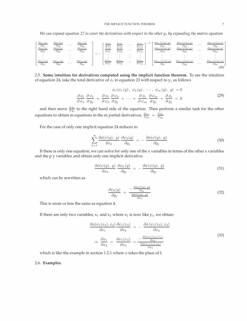
We can expand equation 27 to cover the derivatives with respect to the other y` by expanding the matrix equation
∂ψ1(y)∂y1
∂ψ1(y)∂y2
. . .∂ψ1(y)∂yp
∂ψ2(y)∂y1
∂ψ2(y)∂y2
. . .∂ψ2(y)∂yp
......
......
∂ψm(y)∂y1
∂ψm(y)∂y2
. . .∂ψm(y)∂yp
= −
∂ φ1∂ x1
∂ φ1∂ x2
· · · ∂ φ1∂ xm
∂ φ2∂ x1
∂ φ2∂ x2
· · · ∂ φ2∂ xm
......
......
∂ φm∂ x1
∂ φm∂ x2
· · · ∂ φm∂ xm
−1
∂φ1(ψ(y),y)∂y1
∂φ1(ψ(y),y)∂y2
. . .∂φ1(ψ(y),y)
∂yp∂φ2(ψ(y),y)
∂y1
∂φ2(ψ(y),y)∂y2
. . .∂φ2(ψ(y),y)
∂yp
......
......
∂φm (ψ(y),y)∂y1
∂φm(ψ(y),y)∂y2
. . .∂φm(ψ(y),y)
∂yp
(28)
2.5. Some intuition for derivatives computed using the implicit function theorem. To see the intuitionof equation 24, take the total derivative of φi in equation 23 with respect to yj as follows
φi (ψ1 (y) , ψ2 (y) , · · · , ψm (y) , y) = 0∂ φi∂ ψ1
∂ ψ1
∂ yj+
∂ φi∂ ψ2
∂ ψ2
∂ yj+ · · · +
∂ φi∂ ψm
∂ ψm∂ yj
+∂ φi∂ yj
= 0(29)
and then move ∂ φi
∂ yjto the right hand side of the equation. Then perform a similar task for the other
equations to obtain m equations in the m partial derivatives, ∂ xi
∂ yj= ∂ ψi
∂ yj
For the case of only one implicit equation 24 reduces to
m∑
k=1
∂φ(ψ(y), y)∂xk
∂ψk(y)∂yj
= − ∂φ(ψ(y), y)∂yj
(30)
If there is only one equation, we can solve for only one of the x variables in terms of the other x variablesand the p y variables and obtain only one implicit derivative.
∂φ(ψ(y), y)∂xk
∂ψk (y)∂yj
= − ∂φ (ψ(y), y)∂yj
(31)
which can be rewritten as
∂ψk(y)∂yj
=− ∂φ(ψ(y), y)
∂yj
∂φ(ψ(y), y)∂xk
(32)
This is more or less the same as equation 4.
If there are only two variables, x1 and x2 where x2 is now like y1, we obtain
∂φ(ψ1(x2), x2)∂x1
∂ψ1(x2)∂x2
= − ∂φ (ψ1(x2), x2)∂x2
⇒ ∂x1
∂x2=
∂ψ1(x2)∂x2
=− ∂φ(ψ1(x2),x2)
∂x2
∂φ(ψ1(x2),x2)∂x1
(33)
which is like the example in section 1.2.1 where φ takes the place of f.
2.6. Examples.

8 THE IMPLICIT FUNCTION THEOREM
2.6.1. One implicit equation with three variables.
φ(x01, x
02, y
0) = 0 (34)
The implicit function theorem says that we can solve equation 34 for x01 as a function of x0
2 and y0, i.e.,
x01 = ψ1(x0
2, y0) (35)
and that
φ(ψ1(x2, y), x2, y) = 0 (36)The theorem then says that
∂φ(ψ1(x2, y), x2, y)∂x1
∂ψ1
∂x2=
−∂φ(ψ1(x2, y), x2, y)∂x2
⇒ ∂φ(ψ1(x2, y), x2, y)∂x1
∂x1(x2, y)∂x2
= − ∂φ(ψ1(x2, y), x2, y)∂x2
⇒ ∂x1(x2, y)∂x2
=− ∂φ(ψ1(x2, y), x2, y)
∂x2
∂φ(ψ1(x2, y), x2, y)∂x1
(37)
2.6.2. Production function example.φ(x0
1, x02, y
0) = 0
y0 − f(x01, x
02) = 0
(38)
The theorem says that we can solve the equation for x01.
x01 = ψ1(x0
2, y0) (39)
It is also true that
φ(ψ1(x2, y), x2, y) = 0
y − f(ψ1(x2, y), x2) = 0(40)
Now compute the relevant derivatives
∂φ(ψ1(x2, y), x2, y)∂x1
= − ∂f(ψ1(x2, y), x2)∂x1
∂φ(ψ1(x2, y), x2, y)∂x2
= −∂f(ψ1(x2, y), x2)
∂x2
(41)
The theorem then says that
∂x1(x2, y)∂x2
= −
[∂φ(ψ1(x2, y), x2, y)
∂x2
∂φ(ψ1(x2, y), x2, y)∂x1
]
= −[
− ∂f(ψ1(x2, y),x2)∂x2
− ∂f(ψ1(x2, y),x2)∂x1
]
= −∂f(ψ1(x2, y),x2)
∂x2
∂f(ψ1(x2, y),x2)∂x1
(42)

THE IMPLICIT FUNCTION THEOREM 9
2.7. General example with two equations and three variables. Consider the following system of equa-tions
φ1(x1, x2, y) = 3x1 + 2x2 + 4y = 0
φ2 (x1, x2, y) = 4x1 + x2 + y = 0(43)
The Jacobian is given by
[∂φ1∂x1
∂φ1∂x2
∂φ2∂x1
∂φ2∂x2
]=
[3 24 1
](44)
We can solve system 43 for x1 and x2 as functions of y. Move y to the right hand side in each equation.
3x1 + 2x2 = −4y (45a)
4x1 + x2 = −y (45b)
Now solve equation 45b for x2
x2 = −y − 4x1 (46)
Substitute the solution to equation 46 into equation 45a and simplify
3x1 + 2(−y − 4x1) = −4y
⇒ 3x1 − 2y − 8x1 = −4y
⇒ −5x1 = −2y
⇒ x1 =25y = ψ1(y)
(47)
Substitute the solution to equation 47 into equation 46 and simplify
x2 = −y − 4[
25y
]
⇒ x2 = − 55y − 8
5y
= − 135y = ψ2(y)
(48)
If we substitute these expressions for x1 and x2 into equation 43 we obtain
φ1
(25y , −
135y, y
)) = 3
[25y
]+ 2
[−
135y
]+ 4y
=65y − 26
5y +
205y
= −205y +
205y = 0
(49)
and
10 THE IMPLICIT FUNCTION THEOREM
φ2
(25y , − 13
5y, y
)) = 4
[25y
]+
[− 13
5y
]+ y
=85y − 13
5y +
55y
=135y − 13
5y = 0
(50)
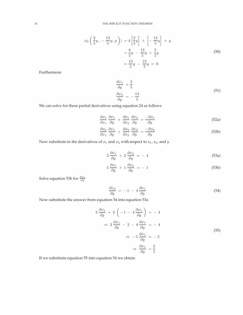
Furthermore
∂ψ1
∂y=
25
∂ψ2
∂y= − 13
5
(51)
We can solve for these partial derivatives using equation 24 as follows
∂φ1
∂x1
∂ψ1
∂y+
∂φ1
∂x2
∂ψ2
∂y=
−∂φ1
∂y(52a)
∂φ2
∂x1
∂ψ1
∂y+
∂φ2
∂x2
∂ψ2
∂y=
−∂φ2
∂y(52b)
Now substitute in the derivatives of φ1 and φ2 with respect to x1, x2, and y.
3∂ψ1
∂y+ 2
∂ψ2
∂y= − 4 (53a)
4∂ψ1
∂y+ 1
∂ψ2
∂y= − 1 (53b)
Solve equation 53b for ∂ψ2∂y
∂ψ2
∂y= − 1 − 4
∂ψ1
∂y(54)
Now substitute the answer from equation 54 into equation 53a
3∂ψ1
∂y+ 2
(− 1 − 4
∂ψ1
∂y
)= − 4
⇒ 3∂ψ1
∂y− 2 − 8
∂ψ1
∂y= − 4
⇒ − 5∂ψ1
∂y= − 2
⇒ ∂ψ1
∂y=
25
(55)
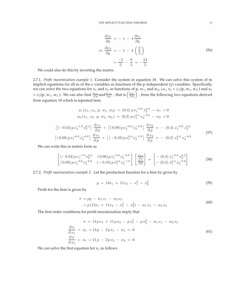
If we substitute equation 55 into equation 54 we obtain
THE IMPLICIT FUNCTION THEOREM 11
∂ψ2
∂y= − 1 − 4
∂ψ1
∂y
⇒ ∂ψ2
∂y= − 1 − 4
(25
)
=−55
− 85
= −135
(56)
We could also do this by inverting the matrix.
2.7.1. Profit maximization example 1. Consider the system in equation 18. We can solve this system of mimplicit equations for all m of the x variables as functions of the p independent (y) variables. Specifically,we can solve the two equations for x1 and x2 as functions of p, w1, and w2, i.e., x1 = ψ1(p, w1, w2 ) and x2
= ψ2(p, w1, w2 ). We can also find ∂ x1∂ p
and∂ x2∂ p
, that is(∂ ψi
∂ p
), from the following two equations derived
from equation 18 which is repeated here.
φ1 (x1, x2, p, w1, w2) = (0.4) p x−0.61 x0.2
2 − w1 = 0
φ2 (x1, x2, p, w1, w2 ) = (0.2) p x0.41 x− 0.8
2 − w2 = 0
[(− 0.24) p x−1.6
1 x0.22
] ∂ x1
∂ p+
[( 0.08) p x−0.6
1 x−0.82
] ∂ x2
∂ p= − (0.4) x−0.6
1 x0.22
[( 0.08) p x−0.6
1 x−0.82
] ∂ x1
∂ p+
[(− 0.16) p x0.4
1 x−1.82
] ∂ x2
∂ p= − (0.2) x0.4
1 x−0.82
(57)
We can write this in matrix form as
[(− 0.24) p x−1.6
1 x0.22 ( 0.08) p x−0.6
1 x− 0.82
( 0.08) p x−0.61 x−0.8
2 (− 0.16) p x0.41 x−1.8
2
] [∂ x1∂ p∂ x2∂ p
]=
[− (0.4) x−0.6
1 x0.22
− (0.2) x0.41 x−0.8
2
](58)
2.7.2. Profit maximization example 2. Let the production function for a firm by given by
y = 14x1 + 11x2 − x21 − x2
2 (59)
Profit for the firm is given by
π = py − w1 x1 − w2 x2
= p (14x1 + 11x2 − x21 − x2
2) − w1 x1 − w2 x2(60)
The first order conditions for profit maximization imply that
π = 14 p x1 + 11 p x2 − p x21 − p x2
2 − w1 x1 − w2 x2
∂ π
∂ x1= φ1 = 14 p − 2 p x1 − w1 = 0
∂ π
∂ x2= φ1 = 11 p − 2 p x2 − w2 = 0
(61)
We can solve the first equation for x1 as follows

12 THE IMPLICIT FUNCTION THEOREM
∂ π
∂ x1= 14 p − 2 p x1 − w1 = 0
⇒ 2 p x1 = 14 p − w1
⇒ x1 =14 p − w1
2 p
= 7 − w1
2 p
(62)
In a similar manner we can find x2 from the second equation
∂ π
∂ x2= 11 p − 2 p x2 − w2 = 0
⇒ 2 p x2 = 11 p − w2
⇒ x2 =11 p − w2
2 p
= 5.5 − w2
2 p
(63)
We can find the derivatives of x1 and x2 with respect to p, w1 and w2 directly as follows:
x1 = 7 − 12w1 p
−1
x2 = 5.5 − 12w2 p
−1
∂ x1
∂ p=
12w1 p
−2
∂ x1
∂ w1= − 1
2p−1
∂ x1
∂ w2= 0
∂ x2
∂ p=
12w2 p
−2
∂ x2
∂ w2= − 1
2p−1
∂ x2
∂ w2= 0
(64)
We can also find these derivatives using the implicit function theorem. The two implicit equations are
φ1(x1, x2, p, w1, w2) = 14 p − 2 p x1 − w1 = 0
φ2(x1, x2 p, w1, w2) = 11 p − 2 p x2 − w2 = 0(65)
First we check the Jacobian of the system. It is obtained by differentiating φ1 and φ2 with respect to x1
and x2 as follows
J =
[∂ φ1∂ x1
∂ φ1∂ x2
∂ φ2∂ x1
∂ φ2∂ x2
]=
[−2 p 0
0 −2p
](66)
The determinant is 4p2 which is positive. Now we have two equations we can solve using the implicitfunction theorem. The theorem says
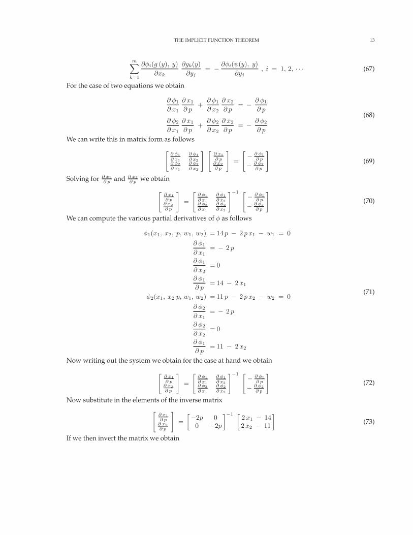
THE IMPLICIT FUNCTION THEOREM 13
m∑
k=1
∂φi(g (y), y)∂xk
∂gk(y)∂yj
= −∂φi(ψ(y), y)
∂yj, i = 1, 2, · · · (67)
For the case of two equations we obtain
∂ φ1
∂ x1
∂ x1
∂ p+
∂ φ1
∂ x2
∂ x2
∂ p= − ∂ φ1
∂ p
∂ φ2
∂ x1
∂ x1
∂ p+
∂ φ2
∂ x2
∂ x2
∂ p= − ∂ φ2
∂ p
(68)
We can write this in matrix form as follows
[∂ φ1∂ x1
∂ φ1∂ x2
∂ φ2∂ x1
∂ φ2∂ x2
] [∂ x1∂ p∂ x2∂ p
]=
[− ∂ φ1
∂ p
− ∂ φ2∂ p
](69)
Solving for ∂ x1∂ p and ∂ x2
∂ p we obtain
[∂ x1∂ p∂ x2∂ p
]=
[∂ φ1∂ x1
∂ φ1∂ x2
∂ φ2∂ x1
∂ φ2∂ x2
]−1 [− ∂ φ1
∂ p
− ∂ φ2∂ p
](70)
We can compute the various partial derivatives of φ as follows
φ1(x1, x2, p, w1, w2) = 14 p − 2 p x1 − w1 = 0∂ φ1
∂ x1= − 2 p
∂ φ1
∂ x2= 0
∂ φ1
∂ p= 14 − 2x1
φ2(x1, x2 p, w1, w2) = 11 p − 2 p x2 − w2 = 0∂ φ2
∂ x1= − 2 p
∂ φ2
∂ x2= 0
∂ φ1
∂ p= 11 − 2x2
(71)
Now writing out the system we obtain for the case at hand we obtain
[∂ x1∂ p∂ x2∂ p
]=
[∂ φ1∂ x1
∂ φ1∂ x2
∂ φ2∂ x1
∂ φ2∂ x2
]−1 [− ∂ φ1
∂ p
− ∂ φ2∂ p
](72)
Now substitute in the elements of the inverse matrix[∂ x1∂ p∂ x2∂ p
]=
[−2p 00 −2p
]−1 [2x1 − 142x2 − 11
](73)
If we then invert the matrix we obtain

14 THE IMPLICIT FUNCTION THEOREM
[∂ x1∂ p∂ x2∂ p
]=
[− 12p 00 − 1
2p
] [2x1 − 142x2 − 11
]
=
[7 − x1p
5.5 − x2p
] (74)
Given thatx1 = 7 − 1
2w1 p
−1
x2 = 5.5 − 12w2 p
−1(75)
we obtain
∂ x1
∂ p=
7 − x1
p
=7 − (7 − 1
2 w1 p−1)
p
=12w1 p
−2
∂ x2
∂ p=
5.5 − x2
p
=5.5 − (5.5 − 1
2w2 p
−1)p
=12w2 p
−2
(76)
which is the same as before.
2.7.3. Profit maximization example 3. Verify the implicit function theorem derivatives ∂ x1∂ w1
, ∂ x1∂ w2
, ∂ x2∂ w1
, ∂ x2∂ w2
for the profit maximization example 2.
2.7.4. Profit maximization example 4. A firm sells its output into a perfectly competitive market and faces afixed price p. It hires labor in a competitive labor market at a wage w, and rents capital in a competitivecapital market at rental rate r. The production is f(L, K). The production function is strictly concave. Thefirm seeks to maximize its profits which are
π = pf(L, K) − wL − rK (77)The first-order conditions for profit maximization are
πL = p fL(L∗, K∗) − w = 0
πK = p fK(L∗, K∗) − r = 0(78)
This gives two implicit equations for K and L. The second order conditions are
∂2 π
∂L2(L∗, K∗) < 0,
∂2 π
∂L2
∂2 π
∂K2−
[∂2 π
∂L∂K
] 2
> 0 at (L∗, K∗) (79)
We can compute these derivatives as
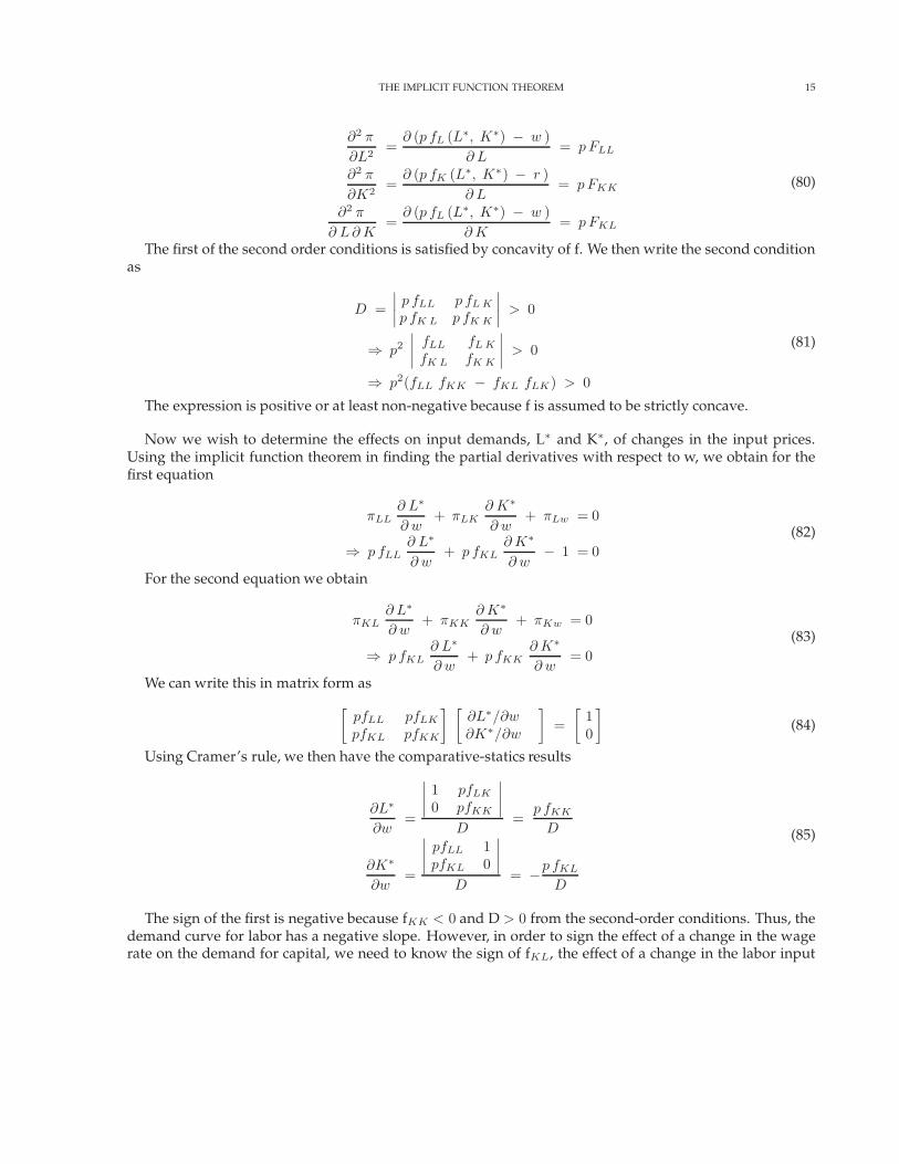
THE IMPLICIT FUNCTION THEOREM 15
∂2 π
∂L2=∂ (p fL (L∗, K∗) − w )
∂ L= pFLL
∂2 π
∂K2=∂ (p fK (L∗, K∗) − r )
∂ L= pFKK
∂2 π
∂ L∂ K=∂ (p fL (L∗, K∗) − w )
∂ K= pFKL
(80)
The first of the second order conditions is satisfied by concavity of f. We then write the second conditionas
D =∣∣∣∣p fLL p fLKp fK L p fKK
∣∣∣∣ > 0
⇒ p2
∣∣∣∣fLL fLKfK L fKK
∣∣∣∣ > 0
⇒ p2(fLL fKK − fKL fLK) > 0
(81)
The expression is positive or at least non-negative because f is assumed to be strictly concave.
Now we wish to determine the effects on input demands, L∗ and K∗, of changes in the input prices.Using the implicit function theorem in finding the partial derivatives with respect to w, we obtain for thefirst equation
πLL∂ L∗
∂ w+ πLK
∂ K∗
∂ w+ πLw = 0
⇒ p fLL∂ L∗
∂ w+ p fKL
∂ K∗
∂ w− 1 = 0
(82)
For the second equation we obtain
πKL∂ L∗
∂ w+ πKK
∂ K∗
∂ w+ πKw = 0
⇒ p fKL∂ L∗
∂ w+ p fKK
∂ K∗
∂ w= 0
(83)
We can write this in matrix form as[pfLL pfLKpfKL pfKK
] [∂L∗/∂w∂K∗/∂w
]=
[10
](84)
Using Cramer’s rule, we then have the comparative-statics results
∂L∗
∂w=
∣∣∣∣1 pfLK0 pfKK
∣∣∣∣D
=p fKKD
∂K∗
∂w=
∣∣∣∣pfLL 1pfKL 0
∣∣∣∣D
= −p fKLD
(85)
The sign of the first is negative because fKK < 0 and D > 0 from the second-order conditions. Thus, thedemand curve for labor has a negative slope. However, in order to sign the effect of a change in the wagerate on the demand for capital, we need to know the sign of fKL, the effect of a change in the labor input

16 THE IMPLICIT FUNCTION THEOREM
on the marginal product of capital. We can derive the effects of a change in the rental rate of capital in asimilar way.
2.7.5. Profit maximization example 5. Let the production function be Cobb-Douglas of the form y = Lα Kβ .Find the comparative-static effects ∂L∗/∂w and ∂K∗/∂w. Profits are given by
π = p f (L, K) − wL − rK
= pLαKβ − wL − rK(86)
The first-order conditions are for profit maximization are
πL = αpLα−1Kβ − w = 0
πK = β pLαKβ− 1 − r = 0(87)
This gives two implicit equations for K and L. The second order conditions are
∂2 π
∂L2(L∗, K∗) < 0,
∂2 π
∂L2
∂2 π
∂K2−
[∂2 π
∂L∂K
] 2
> 0 at (L∗, K∗) (88)
We can compute these derivatives as
∂2 π
∂L2= α (α − 1) p Lα− 2Kβ
∂2 π
∂K2≡ β (β − 1) p LαKβ −2
∂2 π
∂ L∂ K= αβ p Lα−1Kβ−1
(89)
The first of the second order conditions is satisfied as long asα, β < 1. We can write the second conditionas
D =∣∣∣∣α (α − 1) p Lα− 2Kβ αβ p Lα−1Kβ− 1
αβ p Lα− 1Kβ−1 β (β − 1) p LαKβ−2
∣∣∣∣ > 0 (90)
We can simplify D as follows
D =∣∣∣∣α (α − 1) p Lα− 2Kβ αβ p Lα−1Kβ− 1
αβ p Lα−1Kβ− 1 β (β − 1) p LαKβ− 2
∣∣∣∣
= p2
∣∣∣∣α (α − 1) Lα−2Kβ αβ Lα− 1Kβ−1
αβ Lα− 1Kβ− 1 β (β − 1) LαKβ −2
∣∣∣∣= p2
[α β (α − 1) (β − 1) Lα− 2 Kβ LαKβ− 2 − α2 β2 L2α− 2K2β−2
]
= p2[α β Lα− 2 Kβ LαKβ− 2 ( (α − 1) (β − 1) − αβ )
]
= p2[α β Lα− 2 Kβ LαKβ− 2 ( αβ − β − α + 1 − αβ )
]
= p2[α β Lα− 2 Kβ LαKβ− 2 ( 1 − α − β )
]
(91)
The condition is then that
D = p2 αβ L2α−2 K2β−2 (1 − α − β) > 0 (92)
This will be true if α+β < 1.

THE IMPLICIT FUNCTION THEOREM 17
Now we wish to determine the effects on input demands, L∗ and K∗, of changes in the input prices.Using the implicit function theorem in finding the partial derivatives with respect to w, we obtain for thefirst equation
πLL∂ L∗
∂ w+ πLK
∂ K∗
∂ w+ πLw = 0
⇒ α (α − 1) p Lα−2Kβ ∂ L∗
∂ w+ αβ p Lα− 1Kβ− 1 ∂ K
∗
∂ w− 1 = 0
(93)
For the second equation we obtain
πKL∂ L∗
∂ w+ πKK
∂ K∗
∂ w+ πKw = 0
⇒ αβ p Lα−1Kβ− 1 ∂ L∗
∂ w+ β (β − 1) p LαKβ− 2 = 0
(94)
We can write this in matrix form as[α (α − 1) p Lα− 2Kβ αβ p Lα− 1Kβ− 1
αβ p Lα−1Kβ− 1 β (β − 1) p LαKβ− 2
] [∂L∗/∂w∂K∗/∂w
]=
[10
](95)
Using Cramer’s rule, we then have the comparative-statics results
∂L∗
∂w=
∣∣∣∣1 αβ p Lα− 1Kβ−1
0 β (β − 1) p LαKβ− 2
∣∣∣∣D
=β (β − 1) p LαKβ −2
D
∂K∗
∂w=
∣∣∣∣α (α − 1) p Lα−2Kβ 1αβ p Lα−1Kβ− 1 0
∣∣∣∣D
=−αβ p Lα−1Kβ− 1
D
(96)
The sign of the first of is negative because p β (β − 1)LαKβ −2 < 0 (β < 1), and D > 0 by the secondorder conditions. The cross partial derivative ∂K∗
∂w is also less than zero because pαβ Lα− 1Kβ− 1 > 0and D > 0. So, for the case of a two-input Cobb-Douglas production function, an increase in the wageunambiguously reduces the demand for capital.
3. TANGENTS TO φ(x1 , x2 , . . . , ) = c AND PROPERTIES OF THE GRADIENT
3.1. Direction numbers.
A direction in <2 is determined by an ordered pair of two numbers (a,b), not both zero, called directionnumbers. The direction corresponds to all lines parallel to the line through the origin (0,0) and the point(a,b). The direction numbers (a,b) and the direction numbers (ra,rb) determine the same direction, for anynonzero r.
A direction in <n is determined by an ordered n-tuple of numbers(x0
1, x02, . . . , x
0n
), not all zero, called di-
rection numbers. The direction corresponds to all lines parallel to the line through the origin (0,0, . . . ,0) andthe point
(x0
1, x02, . . . , x
0n
). The direction numbers
(x0
1, x02, . . . , x
0n
)and the direction numbers
(rx0
1, rx02, . . . , rx
0n
)
determine the same direction, for any nonzero r. If pick an r in the following way.
|r| =1√
(x01)2 + (x0
2)2 + . . . + (x0n)2
=1
|x0| (97)
then

18 THE IMPLICIT FUNCTION THEOREM
cos γ1 =x0
1√(x0
1)2 + (x02)2 + . . . + (x0
n)2
cos γ2 =x0
2√(x0
1)2 + (x02)2 + . . . + (x0
n)2
...
cos γn =x0n√
(x01)2 + (x0
2)2 + . . . + (x0n)2
(98)
where γj is the angle of the vector running through the origin and the point(x0
1, x02, . . . , x
0n
)with the xj
axis. With this choice of r, the direction numbers (ra,rb) are just the cosines of the angles that the line makeswith the positive x1,x2, . . . and xn axes. These angles γ1, γ2 , . . . are called the direction angles, and theircosines (cos[γ1], cos[γ2], . . . ) are called the direction cosines of that direction. See figure 1. They satisfy
cos2[γ1] + cos2[γ2] + . . . + cos2[γn] = 1
FIGURE 1. Direction numbers as cosines of vector angles with the respective axes
0
1
x1
0
0.5
1x2
0
0.5
1
x3
H 0,0,0 L
x1
x2
x3
x0
0
0.5
x2
From equation 98, we can also write
x0 =(x0
1, x02, . . . , x
0n
)=
(|x0| cos[γ1], |x0| cos[γ2], . . . , |x0| cos[γn
)
= |x0| (cos[γ1], cos[γ2], . . . , cos[γn])(99)
Therefore
THE IMPLICIT FUNCTION THEOREM 19
1|x0|x
0 = (cos[γ1], cos[γ2], . . . , cos[γn]) (100)
which says that the direction cosines of x0 are the components of the unit vector in the direction of x0.
Theorem 3. Ifθ is the angle between the vectors ~a abd~b, then
a · b = |a| |b| cos θ (101)
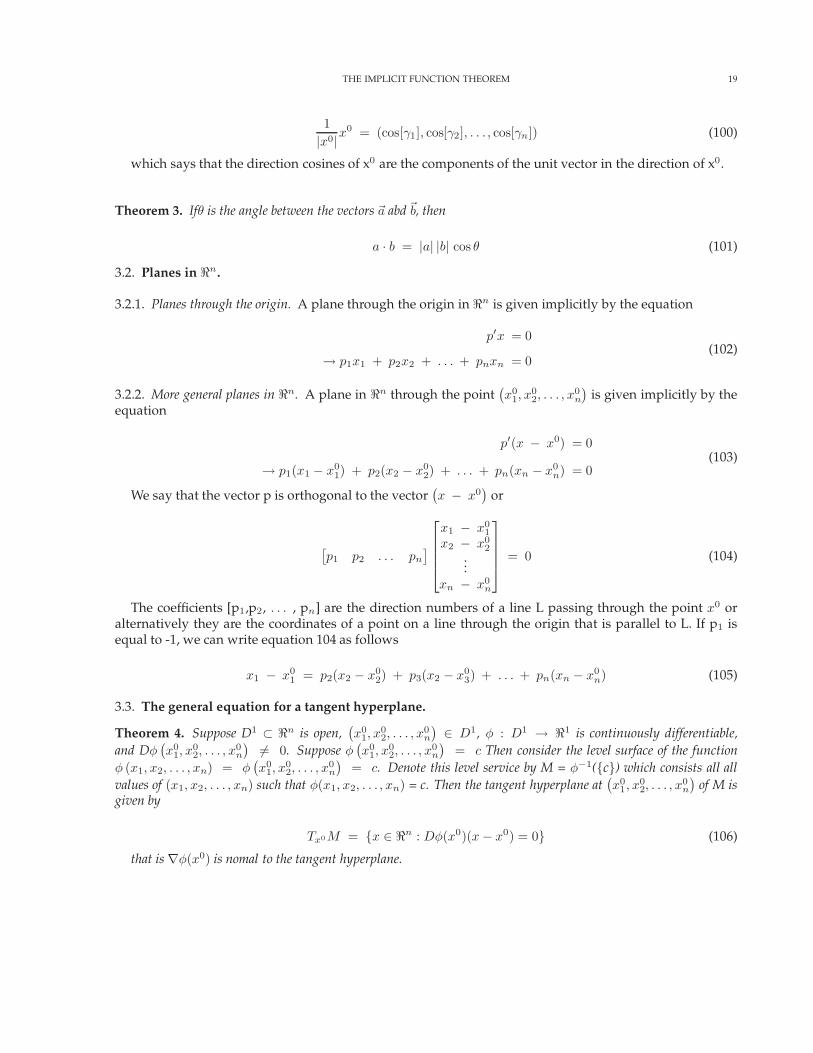
3.2. Planes in <n.
3.2.1. Planes through the origin. A plane through the origin in <n is given implicitly by the equation
p′x = 0
→ p1x1 + p2x2 + . . . + pnxn = 0(102)
3.2.2. More general planes in <n. A plane in <n through the point(x0
1, x02, . . . , x
0n
)is given implicitly by the
equation
p′(x − x0) = 0
→ p1(x1 − x01) + p2(x2 − x0
2) + . . . + pn(xn − x0n) = 0
(103)
We say that the vector p is orthogonal to the vector(x − x0
)or
[p1 p2 . . . pn
]
x1 − x01
x2 − x02
...xn − x0
n
= 0 (104)
The coefficients [p1,p2, . . . , pn] are the direction numbers of a line L passing through the point x0 oralternatively they are the coordinates of a point on a line through the origin that is parallel to L. If p1 isequal to -1, we can write equation 104 as follows
x1 − x01 = p2(x2 − x0
2) + p3(x2 − x03) + . . . + pn(xn − x0
n) (105)
3.3. The general equation for a tangent hyperplane.
Theorem 4. Suppose D1 ⊂ <n is open,(x0
1, x02, . . . , x
0n
)∈ D1, φ : D1 → <1 is continuously differentiable,
and Dφ(x0
1, x02, . . . , x
0n
)6= 0. Suppose φ
(x0
1, x02, . . . , x
0n
)= c Then consider the level surface of the function
φ (x1, x2, . . . , xn) = φ(x0
1, x02, . . . , x
0n
)= c. Denote this level service by M = φ−1({c}) which consists all all
values of (x1, x2, . . . , xn) such that φ(x1, x2, . . . , xn) = c. Then the tangent hyperplane at(x0
1, x02, . . . , x
0n
)of M is
given by
Tx0M = {x ∈ <n : Dφ(x0)(x− x0) = 0} (106)
that is ∇φ(x0) is nomal to the tangent hyperplane.

20 THE IMPLICIT FUNCTION THEOREM
Proof. Because Dφ(x0) 6= 0, we may assume without loss of generality that ∂φ∂x1
(x0) 6= 0. Apply the implicitfunction theorem (Theorem 1) to the function φ− c. We then know that the level set can be expressed as agraph of the function x1 = ψ1(x2, x3, . . . , xn) for some continuous function ψ1. Now the tangent plane to thegraph x1 = ψ1(x2, x3, . . . , xn) at the point x0 = [ψ1(x0
2, x03, . . . , x
0n), x
02, x
03, . . .x
0n] is the graph of the gradient
Dψ1(x02, x0
3, . . . , x0n) translated so that it passes through x0. Using equation 105 where ∂ψ1
∂xk
(x0
2, x03, . . . , x
0n
)
are the direction numbers we obtain
x1 − x01 =
n∑
k=2
∂ψ1
∂xk
(x0
2, x03, . . . , x
0n
)(xk − x0
k) (107)
Now make the substitution from equation 4 in equation 107 to obtain
x1 − x01 =
n∑
k=2
−
∂φ(ψ1(x02, x
03, ..., x
0n),x0
2, x03, ..., x
0n)
∂xk
∂φ(ψ1(x02, x
03, ..., x
0n),x0
2, x03, ..., x
0n)
∂x1
(xk − x0
k)
=n∑
k=2
−
∂φ(x0)∂xk
∂φ(x0)∂x1
(xk − x0
k)
(108)
Rearrange equation 108 to obtain
n∑
k=2
∂φ(x0)∂xk
(xk − x0k) +
∂φ(x0)∂x1
(x1 − x01) = Dφ(x0)(x− x0) = 0 (109)
�
3.4. Example. Consider a function
y = f (x1, x2, · · · , xn) (110)evaluated at the point (x0
1, x02, · · · , x0
n )
y0 = f (x01, x
02, · · · , x0
n) (111)The equation of the hyperplane tangent to the surface at this point is given by
(y − y0) =∂ f
∂x1(x1 − x0
1) +∂ f
∂x2(x2 − x0
2 ) + · · · +∂ f
∂xn(xn − x0
n)
⇒ ∂ f
∂x1(x1 − x0
1) +∂ f
∂x2(x2 − x0
2 ) + · · · +∂ f
∂xn(xn − x0
n) − ( y − y0) = 0
⇒ f(x1, x2, · · · , xn) = f(x01, x
02, · · · , x0
n) +∂ f
∂x1(x1 − x0
1) +∂ f
∂x2(x2 − x0
2) + · · ·+ ∂ f
∂xn(xn − x0
n)
(112)
where the partial derivatives ∂ f∂xi
are evaluated at (x01, x
02, · · · , x0
n ) . We can also write this as
f (x) − f (x0) = ∇ f (x0) (x − x0) (113)Compare this to the tangent equation with one variable
y − f (x0) = f (x0) (x − x0)
⇒ y = f (x0) + f (x0) (x − x0)(114)
and the tangent plane with two variables

THE IMPLICIT FUNCTION THEOREM 21
y − f(x01, x
02) =
∂ f
∂x1(x1 − x0
1) +∂ f
∂x2(x2 − x0
2)
⇒ y = f(x01, x
02) +
∂ f
∂x1(x1 − x0
1) +∂ f
∂x2(x2 − x0
2)(115)
3.5. Vector functions of a real variable. Let x1, x2, ... ,xn be functions of a variable t defined on an intervalI and write
x(t) = (x1(t), x2(t), . . . , xn(t)) (116)
The function t → x(t) is a transformation from R to Rn and is called a vector function of a real variable.As x runs through I, x(t) traces out a set of points in n-space called a curve. In particular, if we put
x1 (t) = x01 + t a1 , x2 (t) = x0
2 + t a2 , · · · , xn (t) = x0n + t an (117)
the resulting curve is a straight line in n-space. It passes through the point x0 = (x01, x
02, · · · , x0
n ) at t= 0, and it is in the direction of the vector a = ( a1, a2, · · · , an ). We can define the derivative of x(t) as
d x
d t= x (t) =
(d x1(t)d t
,d x2(t)d t
, · · · , d xn(t)d t
)(118)
If K is a curve in n-space traced out by x(t), then x (t) can be interpreted as a vector tangent to K at thepoint t.
3.6. Tangent vectors.
Consider the function r(t) = (x1(t), x2(t), · · · , xn(t) ) and its derivative r (t) = (x1(t), x2(t), . . . , xn(t)).This function traces out a curve in Rn. We can call the curve K. For fixed t,
r (t) = limh → 0
r (t + h) − r (t)h
(119)
If r (t) 6= 0, then for t + h close enough to t, the vector r(t+h) - r(t) will not be zero. As h tends to 0, thequantity r(t+h) - r(t) will come closer and closer to serving as a direction vector for the tangent to the curveat the point P. This can be seen in figure 2
It may be tempting to take this difference as approximation of the direction of the tangent and then takethe limit
limh → 0
[ r (t + h) − r (t) ] (120)
and call the limit the direction vector for the tangent. But the limit is zero and the zero vector has nodirection. Instead we use the a vector that for small h has a greater length, that is we use
r (t + h) − r (t)h
(121)
For any real number h, this vector is parallel to r(t+h) - r(t). Therefore its limit
r (t) = limh → 0
r (t + h) − r (t)h
(122)
can be taken as a direction vector for the tangent line.
22 THE IMPLICIT FUNCTION THEOREM
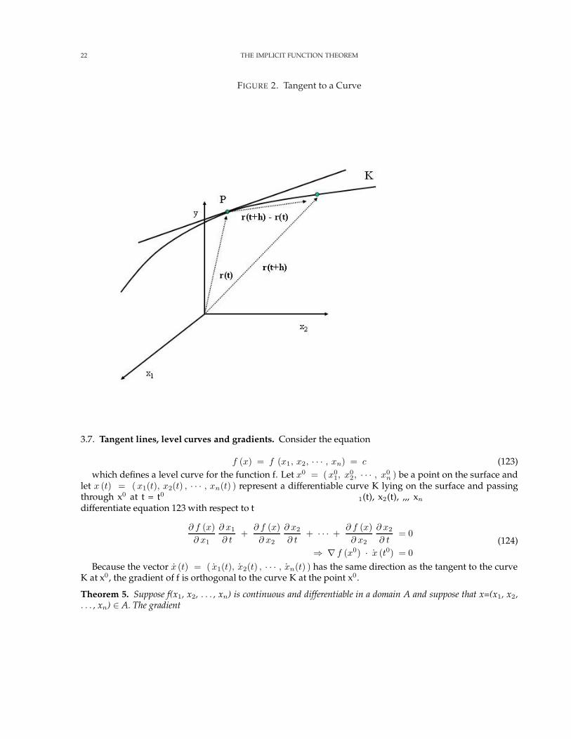
FIGURE 2. Tangent to a Curve
3.7. Tangent lines, level curves and gradients. Consider the equation
f (x) = f (x1, x2, · · · , xn) = c (123)which defines a level curve for the function f. Let x0 = (x0
1, x02, · · · , x0
n ) be a point on the surface andlet x (t) = (x1(t), x2(t) , · · · , xn(t) ) represent a differentiable curve K lying on the surface and passingthrough x0 at t = t0. Because K lies on the surface, f [x(t)] = f [x1(t), x2(t), ,,, xn(t)] = c for all t. Nowdifferentiate equation 123 with respect to t
∂ f (x)∂ x1
∂ x1
∂ t+
∂ f (x)∂ x2
∂ x2
∂ t+ · · · +
∂ f (x)∂ x2
∂ x2
∂ t= 0
⇒ ∇ f (x0) · x (t0) = 0(124)
Because the vector x (t) = ( x1(t), x2(t) , · · · , xn(t) ) has the same direction as the tangent to the curveK at x0, the gradient of f is orthogonal to the curve K at the point x0.
Theorem 5. Suppose f(x1, x2, . . . , xn) is continuous and differentiable in a domain A and suppose that x=(x1, x2,. . . , xn) ∈ A. The gradient

THE IMPLICIT FUNCTION THEOREM 23
∇ f =(∂ f
∂x1,∂ f
∂x2, . . . ,
∂ f
∂xn
)
has the following properties at points x where ∇f(x) 6= 0.(i) ∇f(x) is orthogonal to the level surfaces f(x1, x2, . . . , xn) = c.
(ii) ∇f(x) points in the direction of the steepest increase on f.(iii) ||∇f(x)|| is the value of the directional derivative in the direction of steepest increase.

24 THE IMPLICIT FUNCTION THEOREM
REFERENCES
[1] Hadley, G. Linear Algebra. Reading, MA: Addison-Wesley, 1961.[2] Sydsaeter, Knut. Topics in Mathematical Analysis for Economists. New York: Academic Press, 1981.


![Fixed Point Theorems with Implicit Relations in Fuzzy ... · Singh and S. Jain[15] proved a common fixed point theorem for semicompatible mappings in fuzzy metric space using implicit](https://static.fdocuments.us/doc/165x107/5ede48c0ad6a402d66699b31/fixed-point-theorems-with-implicit-relations-in-fuzzy-singh-and-s-jain15.jpg)

![A Ridiculously Simple and Explicit Implicit Function Theorem · as the Lagrange (or Lagrange–Bu¨rmann) inversion formula [3,7,16,18,34,42,47,48]. What seems to be less well known](https://static.fdocuments.us/doc/165x107/5f0451987e708231d40d632e/a-ridiculously-simple-and-explicit-implicit-function-theorem-as-the-lagrange-or.jpg)
