The impacts of climate change on hydrology in...

Journal of Hydrology (2008) 356, 28–45

ava i lab le at www.sc iencedi rec t . com

journal homepage: www.elsevier .com/ locate / jhydro l

The impacts of climate change on hydrology in Ireland

Susan Steele-Dunne a,b,*, Peter Lynch a, Ray McGrath b, Tido Semmler b,Shiyu Wang b, Jenny Hanafin a,b, Paul Nolan a,b

a Meteorology and Climate Centre, University College Dublin, Belfield, Dublin 4, Irelandb Met Eireann, Glasnevin Hill, Dublin 9, Ireland

Received 31 August 2007; received in revised form 18 March 2008; accepted 21 March 2008

00do

TeReTe

KEYWORDSClimate change;Ireland;Catchment hydrology;Parameter uncertainty;Calibration

22-1694/$ - see front mattei:10.1016/j.jhydrol.2008.03

* Corresponding author. Prchnology, Faculty of Civilsources Section, Postbus 50l.: +31 (0)15 27 81377; fax:E-mail address: s.c.steele-

r ª 200.025

esent aEngineer48, 2600+31 (0)1dunne@t

Summary A study of nine Irish catchments was carried out to quantify the expectedimpact of climate change on hydrology in Ireland. Boundary data from the EuropeanCentre Hamburg Model Version 5 (ECHAM 5) general circulation model were used to forcethe Rossby Centre Atmosphere Model (RCA3) regional climate model, producing dynami-cally downscaled precipitation and temperature data under past and future climatescenarios. This data was used to force the HBV-Light conceptual rainfall-runoff modelto simulate stream flow in the reference period (1961–2000) and in the future(2021–2060) under the Special Report on Emissions Scenarios (SRES) A1B scenario. AMonte-Carlo approach to calibration was used to obtain 100 parameter sets which repro-duced observed stream flow well. Use of an ensemble provided results in terms of a rangerather than a single value. Results suggested an amplification of the seasonal cycle acrossthe country, driven by increased winter precipitation, decreased summer precipitationand increased temperature. The expected changes in mean winter and summer flows aswell as annual maximum daily mean flow varied depending on catchment characteristicsand the timing and magnitude of expected changes in precipitation in each catchment.ª 2008 Elsevier B.V. All rights reserved.

Introduction

From the recent Intergovernmental Panel on ClimateChange (IPCC) Fourth Assessment Report (IPCC, 2007), lit-tle doubt remains that the climate system has warmed in

8 Elsevier B.V. All rights reserved

ddress: Delft University ofing and Geosciences, WaterGA Delft, The Netherlands.5 2785559.udelft.nl (S. Steele-Dunne).

recent decades. Recent observations confirm increases inglobal mean temperatures, rising global average sea leveland diminishing snow and ice cover. This warming, and theconsequent rise in atmospheric water vapor have lead toan increase in mean precipitation over northern Europeas well as an increase in the frequency of heavy precipita-tion events over most land areas. It is expected thatglobal average surface air warming will continue into the21st century, and that hot extremes, heat waves andheavy precipitation events will continue to increase in fre-quency. The objective of this project was to examine how

.

mailto:[email protected]

Figure 1 Locations of study catchments.

Table 1 Stream flow gauge station and location, catch-ment area upstream of the gauge station

Catchment Stream flowgaugestation

Latitude(�N)

Longitude(�E)

Area(km2)

Moy Rahans 54.10 �9.16 1803Boyne Slane Castle 53.71 �6.56 2452Blackwater Ballyduff 52.14 �8.05 2302Suck Bellagill 53.36 �8.24 1219Brosna Ferbane 53.27 �7.83 1210Feale Listowel 52.44 �9.48 648Barrow Royal Oak 52.70 �6.98 2381Suir Clonmel 52.35 �7.70 2138Bandon Curranure 51.77 �8.68 431

The impacts of climate change on hydrology in Ireland 29

the predicted climate change will impact hydrology inIreland.

In recent years, numerous studies have investigated theimpact of climate change on hydrology and water resourcesin many regions (e.g. Arnell and Reynard, 1996; Bergstromet al., 2001; Middelkoop et al., 2001; Gao et al., 2002; Men-zel and Burger, 2002; Pilling and Jones, 2002; Arnell et al.,2003 and Christensen et al., 2004). Charlton et al. (2006)investigate the impact of climate change on water suppliesand flood hazard in Ireland using a grid-based approach,forcing the HYSIM model of Manley (1993) with statisticallydownscaled climate data from the Hadley Centre ClimateModel, HadCM3 (Gordon et al., 2000). Murphy et al.(2006a) employ similarly downscaled data to force HYSIM,modeling individual basins rather than a gridded domain.As they discuss in Murphy et al. (2006b), parameter uncer-tainty is addressed by employing the GLUE methodology ofBeven and Binley (1992) with Latin-Hypercube sampling(McKay et al., 1979) included as an alternative to Monte-Carlo simulations. The key differences between the studypresented here and those of Charlton et al. (2006) and Mur-phy et al. (2006a) are the use of dynamically rather thanstatistically downscaled climate data to force the HBV-Lighthydrology model (Seibert, 2005) and our use of Monte-Carlosimulations to account for parameter uncertainty.

Research carried out under the Community ClimateChange Consortium for Ireland (C4I) project has emphasizeddeveloping dynamically downscaled climate data with whichto investigate climate change and its impacts for Ireland(McGrath et al., 2005; Semmler et al., 2006). A feasibilitystudy was performed by Wang et al. (2006) to explore theexpected change in flood risk for the Suir catchment dueto climate change based on these dynamically downscaleddata. This study builds on the work of Wang et al. (2006)to develop a methodology that will be used with an ensem-ble of dynamically downscaled climate data (Semmleret al., 2006) to investigate the impacts of climate changeon the hydrology of Irish rivers. Wang et al. (2006) usedthe HBV model (Bergstrom, 1992) from the Swedish Meteo-rological and Hydrological Institute (SMHI) which is usuallycalibrated using a manual trial and error approach. Here,it has been replaced by the HBV-Light model of Seibert(2005) because its interface allows Monte-Carlo simulations.Calibration using Monte-Carlo methods yields an ensembleof simulations allowing us to account for parameteruncertainty in our analysis. The second difference is thata significant bias has been identified and reduced in thedynamically downscaled precipitation data. Wood et al.(2004) discuss the occurrence of such biases, and the impactthey can have on this type of study. Thirdly, the scope ofthe study has been expanded to include nine catchments(Fig. 1, Table 1) selected to ensure varying topography,geology, climatology and expected climate change. Finally,the focus has broadened from extreme flooding events to in-clude changes in seasonal flows. Changes in winter and sum-mer flows are of interest in their own right, but also allow usto make more reliable statements about flood risk.

In this study boundary conditions from a general circula-tion model are used to drive a regional climate model toproduce dynamically downscaled precipitation and temper-ature data. These data are used to force a hydrology modelwhich simulates run off during a reference period (1961–

2000) and a future period (2021–2060) for a given futureclimate scenario. In the next section (Study methodology),details of the experiment, including the models and dataused, and a precipitation bias correction scheme are pro-vided. Dynamically downscaled temperature and precipita-tion data are presented to illustrate how climate isexpected to change in Ireland in the future.

The structure of this paper then follows the stages of thestudy methodology, as a successful analysis of the impactsof climate change depends on the successful calibrationand validation of the models. The HBV-Light conceptualhydrology model is forced with observed precipitation and

30 S. Steele-Dunne et al.

temperature data and calibrated using a Monte-Carlo ap-proach. The performance of the hydrology model is thenvalidated by forcing it with dynamically downscaled datafor the reference period (1961–2000) and comparing thesimulated stream flow to observations. When the hydrologymodel has been successfully calibrated and validated, theimpact of climate change on hydrology is simulated by com-paring simulated stream flow in the future (2021–2060) tothat in the reference period. Finally, the conclusions ofthe study are presented and recommended future researchactivities are outlined.

Study methodology

Fig. 2 illustrates the study methodology for each catchmentwhich requires the use of three models. A general circula-tion model (GCM) was first used to simulate global climate.The European Centre Hamburg Model Version 5 (Roeckneret al., 2003) was used here in a coupled atmosphere oceanrun (ECHAM5-OM1). Simulations were carried out by themodel and data group at Max–Planck-Institute for Meteorol-ogy in Hamburg, Germany. The resolution of the GCM is onthe order of hundreds of kilometers. This was too coarse tocapture the fine scale variability in precipitation due toorography and land cover. So, these data were used asboundary condition data to drive a finer resolution RegionalClimate Model (RCM).

The Rossby Centre Regional Atmospheric Climate ModelVersion 3 (RCA3) used here, was developed from the HighResolution Limited Area Model (HIRLAM) but includesimprovements in the radiation scheme, the turbulencescheme and the cloud parameterization (Kjellstrom et al.,2005; Jones et al., 2004). A new land-surface scheme wasdeveloped and implemented in RCA3 (Samuelsson et al.,

Study Meth1) Calibration 2) Valida

Region

HBV-Light conceptua

TME,PME

P

Q

Boundary Condi(1961-2000)

Calibrate HBV-Light model parameters

Validate agai

QME

Observed Flow QOPW Observed

Flow QOPW

Forcing data from Met Éireann>10 year period during 1961-2000

TEC5PAST

Figure 2 Study

2006). In previous work (Semmler et al., 2006; Wanget al., 2006), the RCA3 model was run on a 0.12� (13 km)spherical, rotated latitude/longitude grid encompassing Ire-land, and centered to include the Atlantic Ocean to thenorth, west and south of the country. The use of ECHAM5-OM1 boundary data with RCA3 to derive dynamically down-scaled meteorological data on this grid has been validatedby Wang et al. (2006) and Semmler et al. (2006). In thisstudy, the precipitation and temperature data from thesesimulations were used to examine the impact of climatechange on hydrology in nine catchments in Ireland.

Comparison of dynamically downscaled precipitationdata to gauge data during the reference period revealedbiases of up to 78% in mean monthly and annual precipita-tion. Wood et al. (2004) demonstrate that failure to correctfor bias in downscaled climate forcing data can yieldimplausible results from hydrological models. Experiments(not shown) found that using uncorrected precipitation dataresulted in a bias of up to 50% and 200% in mean winter andsummer streamflow respectively. A simple bias correctionscheme was therefore necessary to provide a more reason-able validation of streamflow during the reference period.Downscaled precipitation data were sorted by month, anda cumulative distribution function (CDF) was calculatedfor each month and compared to observed precipitationdata. The disagreement between the CDFs of simulatedand observed daily precipitation was greatest in the sum-mer, and indicated the occurrence of too many low inten-sity events. A cut-off rate was calculated so that settingall simulated values less than this value to zero correctedthe number of dry days. The magnitude of this cut-off ratevaried from around 0.5 mm day�1 in winter to over2 mm day�1 in summer. The remaining bias was assumedto be evenly distributed over all days with rain andsubtracted. The amount subtracted was typically about

odology3) Climate Change

Studytion

Rossby Centre al Atmospheric Climate Model,

Version 3 (RCA3)

l rainfall run-off model

European Centre Hamburg Model Version 5

(ECHAM5-OM1)

EC5PAST PECFUTURE

EC5PASTQEC5FUTURE

tions Boundary Conditions(2021-2060, A1B Scenario)

nst QOPWExamine impact of climate change on Q

Bias correctionTEC5FUTURE

Methodology.


2.5 mm day�1, though at some stations this was as high as3.5 mm day�1 during the summer months. Higher valueswere typically associated with months and stations withfewer rain days. Implementing this simple scheme reducedthe bias considerably and proved successful in capturingthe seasonal cycle of mean monthly precipitation as wellas its interannual variability. The parameters of the bias re-moval scheme were calculated using the data during thereference period, and were assumed valid for the futureperiod too.

Finally, the dynamically downscaled precipitation andtemperature data provided the required forcing data forthe HBV-Light model (Seibert, 2005) which was used hereto simulate stream flow in nine study catchments (Fig. 1,Table 1). The original HBV model, developed by SMHI(Bergstrom, 1992), is a rainfall-runoff model which includesconceptual numerical descriptions of hydrological processesat the catchment scale. Conceptual models are particularlysuited to this type of study because they have a simplermodel structure than physics-based model, and can thusbe run for lengthy climate simulations. It includes soil andsnow routines, evaporation, linear reservoir equations andchannel routing. Groundwater recharge and actual evapora-tion are functions of actual water storage in a soil box, run-off formation is represented by three linear reservoirequations and channel routing is simulated by a triangularweighting function. Potential evaporation on day t, EPOT(t),is calculated as

EpotðtÞ ¼ ð1þ CETðTðtÞ � TMÞÞEPOT;M ð1Þ

where T(t) is the temperature on day t, TM is the monthlymean temperature and EPOT,M is the monthly mean potentialevaporation. CET is a correction factor obtained throughcalibration. Monthly mean values for potential evaporationand temperature were calculated from observations at thesame synoptic stations used to provide temperature dataduring the calibration period.

The HBV light model (Seibert, 2005) used here has iden-tical structure to the model of Bergstrom (1992), with twosmall changes. The first is inclusion of a spin-up periodrather than requiring prescribed initial states, and secondlythe MAXBAS routing parameter can assume non-integer val-ues. It was used here because its interface permits Monte-Carlo simulations.

Fig. 2 illustrates the three stages in this study. In the firststagetheHBV-Lighthydrologymodelwascalibratedbyforcingit with observed precipitation and comparing the simulatedstreamflow against observations. The second stage was thevalidation stage, in which we demonstrated that the modelsdescribed here can reproduce streamflow during the refer-ence period (1961–2000) when forcedwith simulated precip-itation and temperature data in this period. Finally, thehydrology model was forced with simulated precipitationand temperature data during the future period under a givenclimate scenario and the expected impacts of climate changeon hydrology in the catchments were analyzed.

Expected climate change

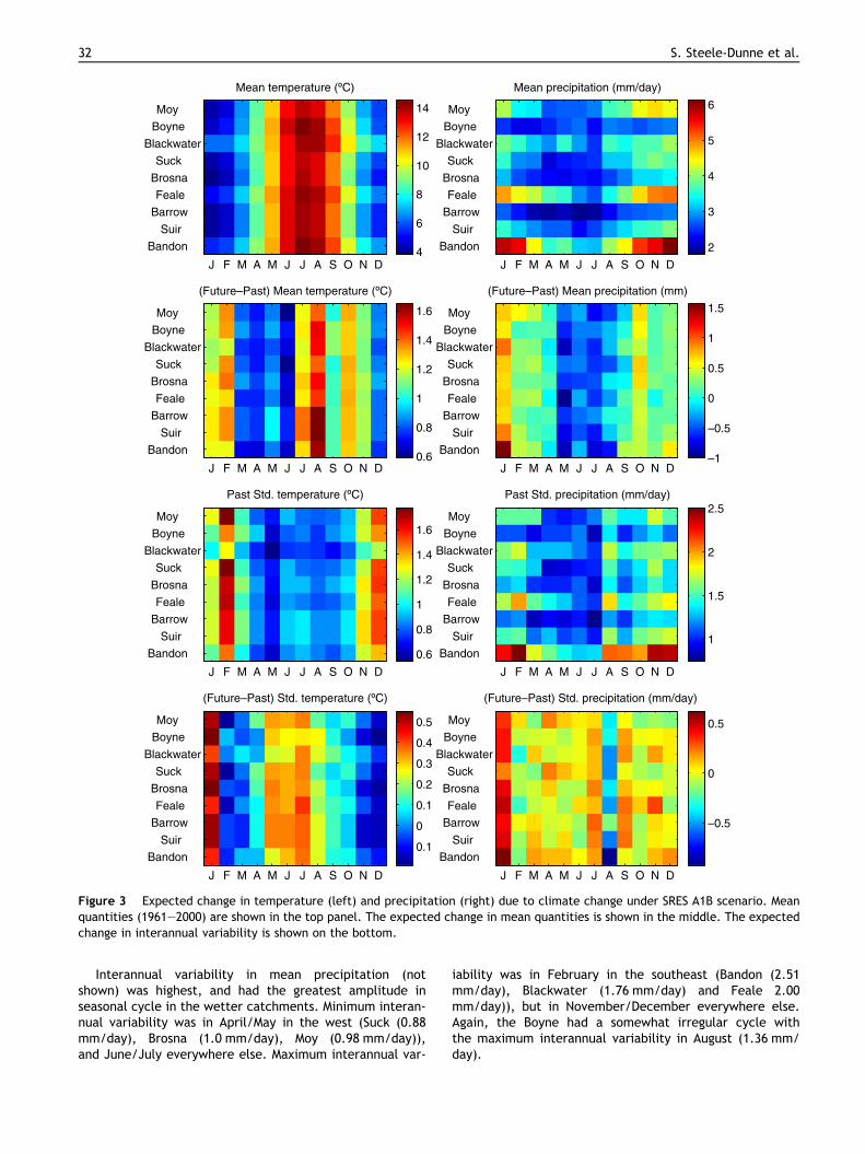
For each of the nine study catchments, Fig. 3 shows themean monthly temperature and precipitation in the refer-

ence period (1961–2000), the expected increase/decreasein these quantities in the period (2021–2060) compared tothe reference period, as well as the expected change ininterannual variability in these quantities between the twoperiods. Future simulations were based on the Special Re-port on Emissions Scenarios (SRES) A1B scenario (Nakicenov-ic et al., 2000), which assumes globalization with strongeconomic growth, and technological emphasis balancedacross all sources (i.e. similar improvement rates apply toall energy supply and end-use technology). Interannual var-iability was calculated as the standard deviation across allyears for each month.

In the reference period 1961–2000, the Blackwater andBandon were the warmest catchments, while the Brosnawas the coolest though the range of mean daily temperatureacross catchments is just 8.91–10.04 �C. There was a strongseasonal cycle in daily mean temperature. In all catch-ments, maximum daily mean temperatures occurred in July(from 13.7 �C in Moy and Suck to 14.5 �C in Boyne) and min-imum daily mean temperatures occurred in January (from3.8 �C in Brosna to 6.2 �C in Blackwater).

Interannual variability in the daily mean temperature foreach month was calculated as the standard deviation inmonthly average daily mean temperature across the 40years of the reference period. Interannual variability inmean daily temperature (not shown) was highest in theBarrow and Suir, and lowest in the Blackwater and exhibiteda strong seasonal cycle. It was highest in February, varyingfrom 1.3 �C Blackwater to 1.8 �C in the Moy and Suck. Inter-annual variability in the summer months was approximatelyhalf that in the winter, and was lowest in May with little var-iation between the catchments.

Under the A1B scenario, temperature is expected toincrease in all months in all catchments. The greatest in-crease is expected in the Barrow and Suir, and the lowestin the Blackwater, though the range across catchments issmall. The greatest increase is expected in August (from1.4 �C in the Moy and Suck to 1.65 �C in the Barrow andSuir). The smallest increase occurs in June and is on the or-der of 0.6–0.7 �C in all catchments.

In general, interannual variability increases betweenApril and October. In winter, there is a decrease in Novem-ber, December and February, while there is an increase ofabout 0.5 �C in January. The greatest decrease is in Decem-ber (�0.07 �C in Blackwater to �0.19 �C in Boyne). In-creased interannual variability in mean daily temperatureaffects potential evapotranspiration, which in turn influ-ences summer low flows and autumn soil moisture.

During the reference period, mean annual precipitationas well as the timing and amplitude of the seasonal cyclewere found to vary with geographical location. The wettestcatchments were the Bandon (1679 mm) and Feale (1469mm) in the southwest. In these catchments the minimumand maximum mean daily precipitation were simulated inJuly (3.13 mm/day, 2.62 mm/day) and December (6.11mm/day, 5.08 mm/day) respectively. The Barrow (849mm) and Boyne (941 mm) were the driest catchments. Inthe southeast the minimum was simulated earlier in June.In the west, the minimum was simulated in April andmaximum in November. The Boyne showed a very irregularseasonal distribution with a minimum (2.2 mm/day) in Feb-ruary and maximum (2.86) in August.

Mean temperature (ºC)

J F M A M J J A S O N D

Moy

Boyne

Blackwater

Suck

Brosna

Feale

Barrow

Suir

Bandon 4

6

8

10

12

14

Mean precipitation (mm/day)


Moy

Boyne

Blackwater

Suck

Brosna

Feale

Barrow

Suir

Bandon 2

3

4

5

6

(Future–Past) Mean temperature (ºC)


Moy

Boyne

Blackwater

Suck

Brosna

Feale

Barrow

Suir

Bandon0.6

0.8

1

1.2

1.4

1.6

(Future–Past) Mean precipitation (mm)


Moy

Boyne

Blackwater

Suck

Brosna

Feale

Barrow

Suir

Bandon–1

–0.5

0

0.5

1

1.5

Past Std. temperature (ºC)


Moy

Boyne

Blackwater

Suck

Brosna

Feale

Barrow

Suir

Bandon 0.6

0.8

1

1.2

1.4

1.6

Past Std. precipitation (mm/day)


Moy

Boyne

Blackwater

Suck

Brosna

Feale

Barrow

Suir

Bandon1

1.5

2

2.5

(Future–Past) Std. temperature (ºC)


Moy

Boyne

Blackwater

Suck

Brosna

Feale

Barrow

Suir

Bandon0.1

0

0.1

0.2

0.3

0.4

0.5

(Future–Past) Std. precipitation (mm/day)


Moy

Boyne

Blackwater

Suck

Brosna

Feale

Barrow

Suir

Bandon

–0.5

0

0.5

Figure 3 Expected change in temperature (left) and precipitation (right) due to climate change under SRES A1B scenario. Meanquantities (1961–2000) are shown in the top panel. The expected change in mean quantities is shown in the middle. The expectedchange in interannual variability is shown on the bottom.


Interannual variability in mean precipitation (notshown) was highest, and had the greatest amplitude inseasonal cycle in the wetter catchments. Minimum interan-nual variability was in April/May in the west (Suck (0.88mm/day), Brosna (1.0 mm/day), Moy (0.98 mm/day)),and June/July everywhere else. Maximum interannual var-

iability was in February in the southeast (Bandon (2.51mm/day), Blackwater (1.76 mm/day) and Feale 2.00mm/day)), but in November/December everywhere else.Again, the Boyne had a somewhat irregular cycle withthe maximum interannual variability in August (1.36 mm/day).


Under the A1B scenario, a general increase in winter pre-cipitation and decrease in summer precipitation is ex-pected. The decrease in precipitation extends from Aprilto August in the southwest, and May to September in thewest, and May to July/August in the east and southeast. Inall catchments the greatest increase is expected in January(from 0.62 mm/day in Boyne to 1.56 mm/day in Bandon).The largest decrease is generally expected in May (from�0.59 mm/day in the Barrow and Brosna to �1.0 mm/dayin the Feale) but occurs later in July for the Moy and Suck.

Little trend was identified in the expected change ininterannual variability in precipitation, which is expectedto increase or decrease by up to 0.2 mm/day. However,all catchments showed an expected decrease in August(from �0.16 mm/day in the Barrow to �0.92 mm/day inBandon) and an increase in January (from 0.2352 mm/dayin Suck to 0.6232 mm/day in Bandon).

HBV-Light model calibration

A defining feature of any conceptual model, such as HBV-Light, is that its parameters are not physically measurable,and must be calibrated (Kavetski et al., 2006). The first stepin this study was to calibrate the HBV-Light model by forcingit with observed precipitation and temperature data fromMet Eireann, the Irish National Meteorological Service. Tem-perature data from the nearest synoptic station to the

Table 2 HBV-Light model parameter definitions, units and reaso

Parameter Definition

FC Maximum value of soil moisture storageLP Fraction of FC above which actual ET equals potenBETA Shape coefficientCET Correction factor for potential evaporationK0 Recession coefficient (upper box)K1 Recession coefficient (upper box)K2 Recession coefficient (lower box)MAXBAS Length of triangular weighting function in routingPERC Maximum rate of recharge between the upper

and lower groundwater boxesUZL Threshold for Q0 flow

Table 3 Calibration period and HBV-Light calibration quality ind

Catchment Calibration Period Me

Moy 01/01/1974–12/31/1983 0.Boyne 01/01/1980–12/31/1991 0.Blackwater 22/06/1965–21/06/1974 0.Suck 01/07/1975–01/06/1984 0.Brosna 01/01/1967–31/12/1976 0.Feale 01/01/1975–31/12/1984 0.Barrow 01/05/1972–30/04/1981 0.Suir 01/01/1975–31/12/1984 0.Bandon 16/02/1975–15/02/1984 0.

Reff refers to the modified Nash-Sutcliffe efficiency parameter. Focalibration.

catchment was used, while precipitation data from 8 to 12rain gauges in the catchment were used to derive a timeseries of mean areal daily precipitation using Theissen poly-gons. Simulated daily mean flow was compared to observedstream flow data from the Office of Public Works (OPW,2007).

The HBV and HBV-Light model parameters are physically-based, but they are effective parameters for the catchmentand may not bear any semblance to measurements from thefield. In the User’s Manual for the original HBV model(Bergstrom, 1992) it is recommended that the model becalibrated manually using a trial and error approach seekingthe unique optimal parameter set that best simulates runoffduring the calibration period. However, conceptual modelsare often over-parameterized, so that very different param-eter sets can give similarly good results during calibration(e.g. Mein and Brown, 1978; Beven and Binley, 1992; Duanet al., 1992; Beven, 1993; Freer et al., 1996; van der Perkand Bierkens, 1997; Seibert et al., 1997). Furthermore,interactions between model parameters may result in thembeing inter-correlated (Jakeman and Hornberger, 1993 andGaume et al., 1998). The run off may be sensitive to changein one uncertain parameter value, but the impact of thechange may be compensated for by other uncertainparameters.

Badly-defined parameters introduce subjectivity in bothmanual and automatic calibration approaches. In a manual

nable ranges for variables which were calibrated in this study

Units Minimum Value Maximum Value

mm 50 500tial ET – 0.3 1.0

– 1.0 6.0C�1 0.0 0.3d�1 0.05 0.5d�1 0.01 0.4d�1 0.001 0.15

routine d 1 7mm d�1 0 3

mm 0 100

icators for each catchment

an (Reff) Max (Reff) 99th percentile

7682 0.9626 0.94717355 0.912 0.88857081 0.8394 0.82467461 0.9235 0.91247338 0.8992 0.87264861 0.7797 0.7276761 0.9229 0.90517341 0.8736 0.8535235 0.7314 0.7133

r each catchment, 10,000 ensemble members were run in the


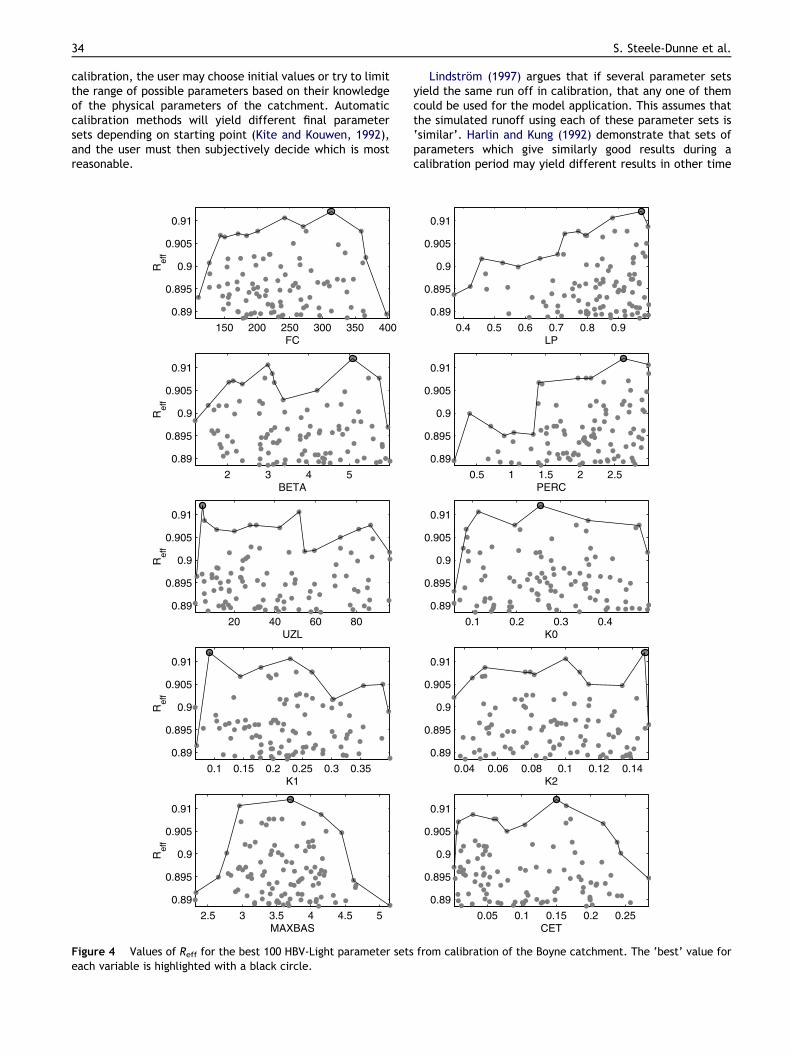
calibration, the user may choose initial values or try to limitthe range of possible parameters based on their knowledgeof the physical parameters of the catchment. Automaticcalibration methods will yield different final parametersets depending on starting point (Kite and Kouwen, 1992),and the user must then subjectively decide which is mostreasonable.

150 200 250 300 350 400

0.89

0.895

0.9

0.905

0.91

FC

Ref

f

2 3 4 5

0.89

0.895

0.9

0.905

0.91

BETA

Ref

f

20 40 60 80

0.89

0.895

0.9

0.905

0.91

UZL

Ref

f

0.1 0.15 0.2 0.25 0.3 0.35

0.89

0.895

0.9

0.905

0.91

K1

Ref

f

2.5 3 3.5 4 4.5 5

0.89

0.895

0.9

0.905

0.91

MAXBAS

Ref

f

Figure 4 Values of Reff for the best 100 HBV-Light parameter setseach variable is highlighted with a black circle.

Lindstrom (1997) argues that if several parameter setsyield the same run off in calibration, that any one of themcould be used for the model application. This assumes thatthe simulated runoff using each of these parameter sets is‘similar’. Harlin and Kung (1992) demonstrate that sets ofparameters which give similarly good results during acalibration period may yield different results in other time

0.4 0.5 0.6 0.7 0.8 0.9

0.89

0.895

0.9

0.905

0.91

LP

0.5 1 1.5 2 2.5

0.89

0.895

0.9

0.905

0.91

PERC

0.1 0.2 0.3 0.4

0.89

0.895

0.9

0.905

0.91

K0

0.04 0.06 0.08 0.1 0.12 0.14

0.89

0.895

0.9

0.905

0.91

K2

0.05 0.1 0.15 0.2 0.25

0.89

0.895

0.9

0.905

0.91

CET

from calibration of the Boyne catchment. The ‘best’ value for


periods. This occurs because model parameters determinethe states of the various submodels, i.e. the soil routine,snow routine, routing routine etc., and so the states ofthe various submodels may differ depending on choice ofparameter set. This is particularly significant in a climateimpact study as the changes in weather conditions will im-pact some subroutines more than others. For example, theimpact of the change in temperature will be determinedby the parameters of the evaporation parameterizationand soil moisture routine. Seibert (1997) argues that usinga Monte-Carlo approach to calibration allows the interactionbetween parameters to be taken into account as wholeparameter sets vary rather than varying individual parame-ters. Furthermore, simulations yield an ensemble of possi-ble results so expected changes can be expressed as arange rather than a single result.

Table 2 contains a list of the parameters calibrated, theirabbreviated name in the model, units and a reasonable

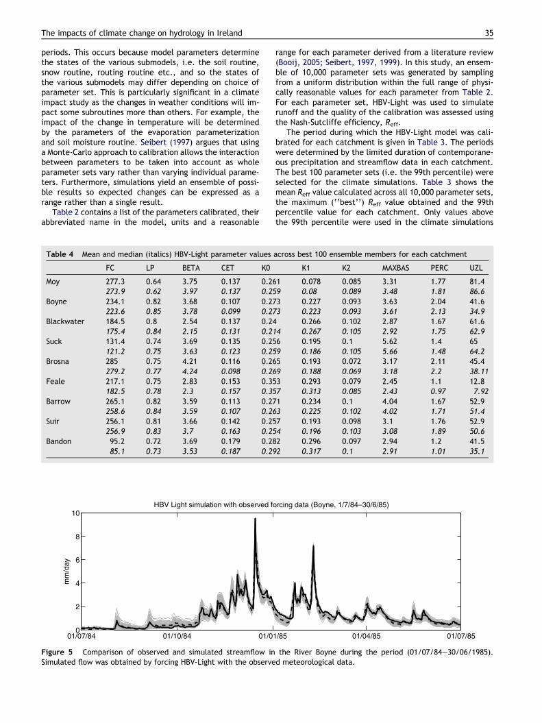
Table 4 Mean and median (italics) HBV-Light parameter values

FC LP BETA CET K0

Moy 277.3 0.64 3.75 0.137 0.26273.9 0.62 3.97 0.137 0.25

Boyne 234.1 0.82 3.68 0.107 0.27223.6 0.85 3.78 0.099 0.27

Blackwater 184.5 0.8 2.54 0.137 0.24175.4 0.84 2.15 0.131 0.21

Suck 131.4 0.74 3.69 0.135 0.25121.2 0.75 3.63 0.123 0.25

Brosna 285 0.75 4.21 0.116 0.26279.2 0.77 4.24 0.098 0.26

Feale 217.1 0.75 2.83 0.153 0.35182.5 0.78 2.3 0.157 0.35

Barrow 265.1 0.82 3.59 0.113 0.27258.6 0.84 3.59 0.107 0.26

Suir 256.1 0.81 3.66 0.142 0.25256.9 0.83 3.7 0.163 0.25

Bandon 95.2 0.72 3.69 0.179 0.2885.1 0.73 3.53 0.187 0.29

01/07/84 01/10/84 01/010

2

4

6

8

10

mm

/day

HBV Light simulation with observed fo

Figure 5 Comparison of observed and simulated streamflow inSimulated flow was obtained by forcing HBV-Light with the observe

range for each parameter derived from a literature review(Booij, 2005; Seibert, 1997, 1999). In this study, an ensem-ble of 10,000 parameter sets was generated by samplingfrom a uniform distribution within the full range of physi-cally reasonable values for each parameter from Table 2.For each parameter set, HBV-Light was used to simulaterunoff and the quality of the calibration was assessed usingthe Nash-Sutcliffe efficiency, Reff.

The period during which the HBV-Light model was cali-brated for each catchment is given in Table 3. The periodswere determined by the limited duration of contemporane-ous precipitation and streamflow data in each catchment.The best 100 parameter sets (i.e. the 99th percentile) wereselected for the climate simulations. Table 3 shows themean Reff value calculated across all 10,000 parameter sets,the maximum (‘‘best’’) Reff value obtained and the 99thpercentile value for each catchment. Only values abovethe 99th percentile were used in the climate simulations

across best 100 ensemble members for each catchment

K1 K2 MAXBAS PERC UZL

1 0.078 0.085 3.31 1.77 81.49 0.08 0.089 3.48 1.81 86.63 0.227 0.093 3.63 2.04 41.63 0.223 0.093 3.61 2.13 34.9

0.266 0.102 2.87 1.67 61.64 0.267 0.105 2.92 1.75 62.96 0.195 0.1 5.62 1.4 659 0.186 0.105 5.66 1.48 64.25 0.193 0.072 3.17 2.11 45.49 0.188 0.069 3.18 2.2 38.113 0.293 0.079 2.45 1.1 12.87 0.313 0.085 2.43 0.97 7.921 0.234 0.1 4.04 1.67 52.93 0.225 0.102 4.02 1.71 51.47 0.193 0.098 3.1 1.76 52.94 0.196 0.103 3.08 1.89 50.62 0.296 0.097 2.94 1.2 41.52 0.317 0.1 2.91 1.01 35.1

/85 01/04/85 01/07/85

rcing data (Boyne, 1/7/84–30/6/85)

the River Boyne during the period (01/07/84–30/06/1985).d meteorological data.

J F M A M J J A S O N D0

0.5

1

1.5

2

2.5

3HBV Light Simulation, Boyne (01/01/1980–12/31/1991)

mm

/day

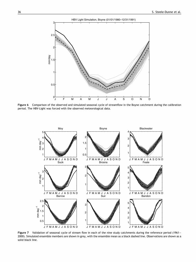
Figure 6 Comparison of the observed and simulated seasonal cycle of streamflow in the Boyne catchment during the calibrationperiod. The HBV-Light was forced with the observed meteorological data.


1

2

3

4

5

mm

day

–1

Moy


0.5

1

1.5

2

Boyne


1

2

3

4Blackwater


1

2

3

mm

day

–1

Suck


1

2

3

Brosna


1

2

3

4

5

Feale


0.5

1

1.5

2

2.5

mm

day

–1

Barrow


1

2

3

Suir


1

2

3

4

5

Bandon

Figure 7 Validation of seasonal cycle of stream flow in each of the nine study catchments during the reference period (1961–2000). Simulated ensemble members are shown in grey, with the ensemble mean as a black dashed line. Observations are shown as asolid black line.



presented in the following sections. The best and worst cal-ibrations were obtained in the Moy and Bandon catchments,where the 99th percentile values were 0.9471 and 0.7133respectively.

Calibration results for the Boyne catchment shown inFig. 4 demonstrate the merits of using a Monte-Carlo ap-proach. Usually, when the HBV model is calibrated using atrial and error approach, one parameter is varied within acertain range, while all other parameters are held constant.A parameter was considered sensitive if it yielded very dif-ferent stream flows at different values. Furthermore, theparameter was considered well-defined if the quality ofthe calibration deteriorated as the parameter value devi-ated from some optimum value. For each of the parameterscalibrated, Fig. 4 shows the values of the best 100 parame-ter sets and the Reff value associated with that calibration.Clearly, excellent simulations (Reff > 0.9) were possible overwide ranges of most model parameters.

From Seibert (1997), it is the upper boundaries of thescatter plots that are of real interest, as for any value ofa given parameter, poor simulations may occur due to thevalues of the other parameters. For a well-defined parame-ter, the upper boundary should have a distinct peak while inill-defined parameters the upper boundary will have a broadplateau. In the Boyne catchment LP, PERC and MAXBAS werethe best defined parameters. It is noteworthy that the list ofwell-defined parameters was found to vary by catchment.

101

3

4

5

6

mm

day

–1

Moy

1

2

3

Boy

101

2

3

4

5

6

mm

day

–1

Suck

2

3

4

Bro

101

2

3

4

Return Period (year)

mm

day

–1

Barrow

2

3

4

5

6

Return Pe

Su

Figure 8 Validation of simulated mean winter flow during the rewinter (DJF) for each year. Ensemble members are shown in grey, thas black asterisks.

For each parameter, the mean and median values calcu-lated across the 100 ensemble members used in the climatesimulations are shown in Table 4. These values do not rep-resent the optimal parameter set, but merely provides away of qualitatively comparing the catchments.

Large values of FC and BETA are associated with moredamped and even hydrographs (e.g. Brosna, Moy, Suir,Boyne, and Barrow). However, steep slopes and the absenceof extensive aquifers can explain large values of BETA in thesmaller river catchments like the Bandon, because BETA canalso be interpreted as a measure of the extension of relativecontributing area (Seibert et al., 2000). Low values of CETare associated with more damped and even hydrographs(e.g. Boyne, Barrow and Brosna). The recession coefficients(K0, K1 and K2) can be expected to decrease with increasingcatchment size because of a more damped and even hydro-graph in a larger catchment. This is at least true for K1which has its highest values in the Bandon and Feale, andmuch lower values in larger catchments such as the Boyneand Suir. Flow from the lower groundwater box is limitedto PERC, so small values (e.g. Feale, Bandon) result in a lar-ger response from the upper groundwater box. MAXBAS canbe expected to increase with increasing catchment size be-cause of the increasing channel length (e.g. Suck, Boyne,and Barrow).

Fig. 5 shows the simulated streamflow in the the riverBoyne for a year during the calibration period for the best

101

ne

101

2

3

4

5

6Blackwater

101

sna

101

4

6

8

Feale

101

riod (year)

ir

101

2

4

6

8


Bandon

ference period (1961–2000). Daily mean flow is averaged overe ensemble mean as a black circle, and observations are shown


100 ensemble members, using the observed meteorologicaldata to force the HBV-Light model. Fig. 5 demonstrates thatthe model is capable of reproducing the observed flow quitewell. Ensemble spread is low relative to the dynamic rangeof values. The observations fall within the ensemble onalmost all days. It can be seen however, that there weresome discrepancies between the simulated and observedflow, particularly during the winter peaks which are oftenunderestimated. Fig. 6 compares the simulated and ob-served seasonal cycle of streamflow calculated from the fullcalibration period. Clearly, even when forced with ‘good’calibration data, the HBV-Light model is not perfect. In bothFigs. 5 and 6, observations are generally closer to the upperlimit of ensemble spread, with large events, and conse-quently winter flows underestimated.

Validation of past climate (1961–2000)

Calibration produced 100 parameter sets which producedsatisfactory agreement between simulated and observedflow during the calibration period. However, this does notguarantee that simulated flow in other time periods, orforced with other data, will agree with observations. Whenthe HBV-Light model parameters for a catchment werefound, the stream flow generated using the past climatedata (1961–2000) was validated against observations.Boundary conditions from the ECHAM5-OM1 model during

101

0.5

1

1.5

2

mm

day

–1

Moy

0.5

1

1.5

Bo

101

0.5

1

1.5

2

mm

day

–1

Suck

0.5

1

1.5

Br

101

0.20.40.60.8

11.21.4


mm

day

–1

Barrow

0.5

1

1.5

2

Return P

S

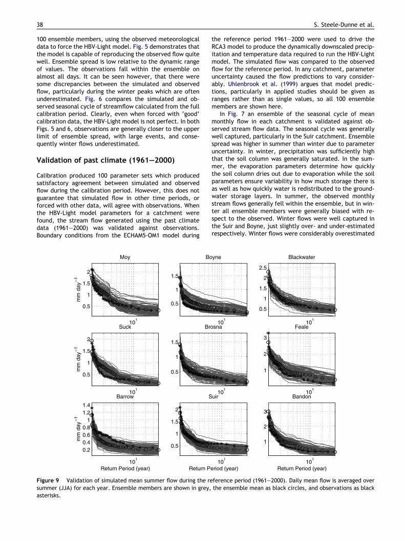
Figure 9 Validation of simulated mean summer flow during the rsummer (JJA) for each year. Ensemble members are shown in grey,asterisks.

the reference period 1961–2000 were used to drive theRCA3 model to produce the dynamically downscaled precip-itation and temperature data required to run the HBV-Lightmodel. The simulated flow was compared to the observedflow for the reference period. In any catchment, parameteruncertainty caused the flow predictions to vary consider-ably. Uhlenbrook et al. (1999) argues that model predic-tions, particularly in applied studies should be given asranges rather than as single values, so all 100 ensemblemembers are shown here.

In Fig. 7 an ensemble of the seasonal cycle of meanmonthly flow in each catchment is validated against ob-served stream flow data. The seasonal cycle was generallywell captured, particularly in the Suir catchment. Ensemblespread was higher in summer than winter due to parameteruncertainty. In winter, precipitation was sufficiently highthat the soil column was generally saturated. In the sum-mer, the evaporation parameters determine how quicklythe soil column dries out due to evaporation while the soilparameters ensure variability in how much storage there isas well as how quickly water is redistributed to the ground-water storage layers. In summer, the observed monthlystream flows generally fell within the ensemble, but in win-ter all ensemble members were generally biased with re-spect to the observed. Winter flows were well captured inthe Suir and Boyne, just slightly over- and under-estimatedrespectively. Winter flows were considerably overestimated

101

yne

101

0.5

1

1.5

2

2.5

Blackwater

101

osna

101

1

2

3

Feale

101

eriod (year)

uir

101

1

2

3


Bandon

eference period (1961–2000). Daily mean flow is averaged overthe ensemble mean as black circles, and observations as black


in the Suck, Barrow, Brosna and Bandon and significantlyunderestimated in the Moy, Blackwater and Feale. Summerflow was generally better modeled than winter flow, withthe only serious discrepancies in the Boyne (overestimated)and the Barrow (underestimated). Differences between sim-ulated and observed streamflow are due to the imperfectHBV-Light model (Figs. 5 and 6), as well as errors in thedownscaled forcing data from the ECHAM5-OM1/RCA3simulations.

In Fig. 8 the modeled mean winter (DJF) stream flow isplotted as a function of return period for each of thecatchments and compared against observations from theOPW. If some winter flow Q20 has a return period of 20years, then mean winter flow is likely to exceed this amounton average once every 20 years. Equivalently, in any yearthere is a 5% chance that mean winter flow will exceed thisamount. This quantity was very reliably estimated, withexcellent agreement in the Suir, Boyne and Bandon catch-ments. Risk was overestimated in the Suck, Barrow and Bro-sna. Recall from Fig. 7 that these were the catchments inwhich mean monthly flows were overestimated in winter.Risk was underestimated in the Moy, Blackwater and Feale,the catchments in which summer monthly flows were under-estimated. Ensemble spread was typically just 10–15% ofthe range of all values indicating that the effects of param-eter uncertainty are pretty insignificant in this quantity.However, in the biased results the observations typically felloutside the ensemble. Errors were as high as 50% (Brosna).

101

5

10

15

20

Moy

Flo

w(m

m d

ay–1

5

10

15

20

Bo

Flo

w(m

m d

ay1

101

5

10

15

20

25Suck

Flo

w(m

m d

ay–1

5

10

15

20

25

Br

Flo

w(m

m d

ay1

101

5

10

15

20

25

Barrow

Return Period (yr)

Flo

w(m

m d

ay–1

10

20

30

S

Return

Flo

w(m

m d

ay1

Figure 10 Validation of simulated annual maximum daily mean floare shown in grey, the ensemble mean as black circles and observe

Fig. 9 shows the modeled mean summer (JJA) streamflow as a function of return period. If some summer flowQ10 has a return period of 10 years, then summer flow willonly be less than this value once in 10 years, or equivalentlythere is a 10% chance that in any given year the mean sum-mer flow will be less than this amount. Ensemble spread wasgenerally much greater than for the mean winter flow case,due again to the greater impact of parameter uncertaintyon summer flows. In all catchments, observations fell withinthe ensemble spread, though the spread in this case wasmuch larger than in the case of the winter flows. Agreementwas generally good, though risk was underestimated in theBoyne, Suck and Feale and overestimated in the Suir andBarrow.

The annual maximum daily mean flow is plotted againstreturn period in Fig. 10. The most striking difference be-tween this and Fig. 8 is that ensemble spread is significantlygreater here. This indicates that while parameter uncer-tainty had little impact on our ability to simulate mean win-ter flow, it had a large influence on simulations of singleevents such as the annual maximum daily mean flow. Thismakes sense as a mean over 90 days will integrate someof the differences in model parameters because it is anaveraged quantity. The maximum value depends on thestates of the model and its various subroutines on a singleday.

Despite the large spread, observations fell outside theensemble in half of the catchments (Suck, Barrow, Brosna,

101

yne

101

5

10

15

20

25

Blackwater

101

osna

101

20

30

40

Feale

101

uir

Period (yr)10

1

20

30

40

Bandon

Return Period (yr)

w during the reference period (1961–2000). Ensemble membersd values as black asterisks.


Feale).The best results were obtained for the Boyne andBandon, which from Fig. 8 were the most reliable simula-tions of mean winter flow return period. Despite excellentagreement with observations in Figs. 7 and 8, simulated an-nual maximum daily mean flow in the Suir was overesti-mated in Fig. 10. In general, with the exception of theFeale, risk was generally overestimated. This occurred de-spite results from Fig. 7 indicating that half of the catch-ments overestimated and half underestimated meanwinter flow.

In Fig. 10, all ensemble members were forced with thesame precipitation data, but the response of the varioussubroutines varied depending on the model parameters.So, assuming that the peak precipitation occurs on the sameday in each ensemble member (which is the case), theensemble spread was due entirely to parameter uncer-tainty. The discrepancy between the observations and theensemble members occurred because the single precipita-tion event which gave rise to the observed maximum wasnot simulated with the same magnitude or at the same timein the climate model. In short, it is unreasonable to expectthe experiment set-up to reproduce single events such asannual maximum daily mean flow as reliably as it can repro-duce averaged quantities such as seasonal flows.

Climate change impacts on hydrology

In this section, the impact of the expected climate changeunder the A1B scenario was examined by comparing stream-


–60

–40

–20

0

%

Moy

J F M A M J

–60

–40

–20

0

20

Bo

J F M A M J J A S O N D–60

–40

–20

0

20

%

Suck

J F M A M J

–60

–40

–20

0

Br


–60

–40

–20

0

20

%

Barrow

J F M A M J

–60

–40

–20

0

S

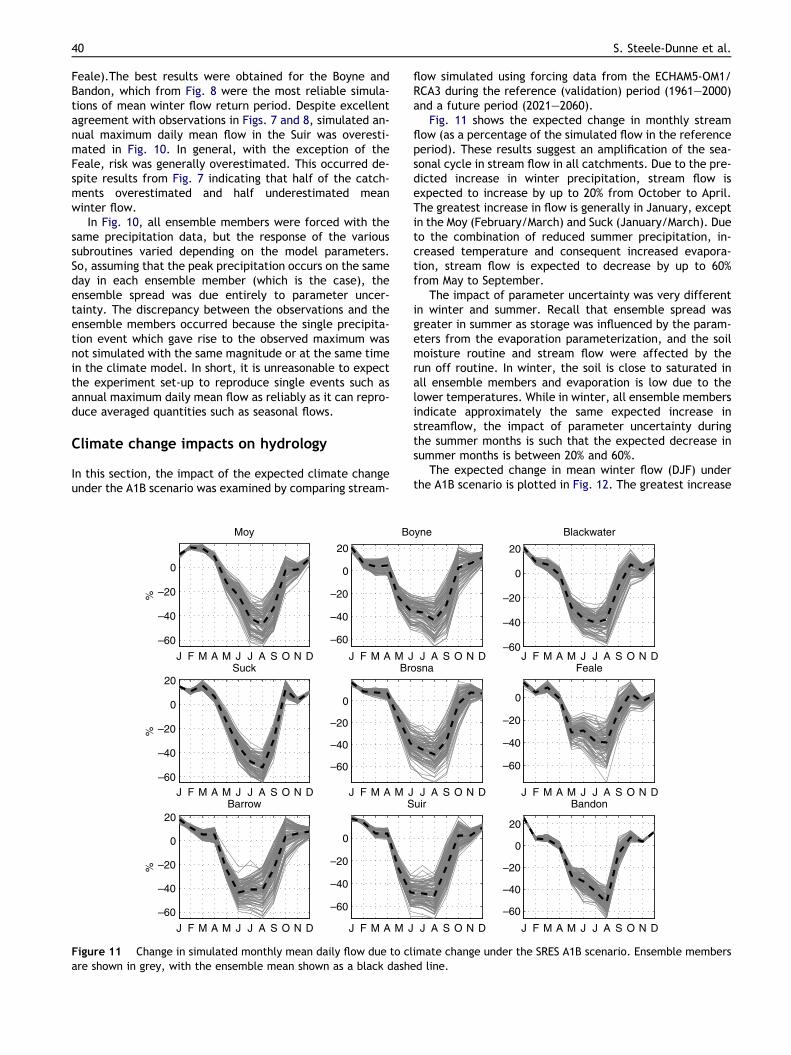
Figure 11 Change in simulated monthly mean daily flow due to clare shown in grey, with the ensemble mean shown as a black dash

flow simulated using forcing data from the ECHAM5-OM1/RCA3 during the reference (validation) period (1961–2000)and a future period (2021–2060).

Fig. 11 shows the expected change in monthly streamflow (as a percentage of the simulated flow in the referenceperiod). These results suggest an amplification of the sea-sonal cycle in stream flow in all catchments. Due to the pre-dicted increase in winter precipitation, stream flow isexpected to increase by up to 20% from October to April.The greatest increase in flow is generally in January, exceptin the Moy (February/March) and Suck (January/March). Dueto the combination of reduced summer precipitation, in-creased temperature and consequent increased evapora-tion, stream flow is expected to decrease by up to 60%from May to September.

The impact of parameter uncertainty was very differentin winter and summer. Recall that ensemble spread wasgreater in summer as storage was influenced by the param-eters from the evaporation parameterization, and the soilmoisture routine and stream flow were affected by therun off routine. In winter, the soil is close to saturated inall ensemble members and evaporation is low due to thelower temperatures. While in winter, all ensemble membersindicate approximately the same expected increase instreamflow, the impact of parameter uncertainty duringthe summer months is such that the expected decrease insummer months is between 20% and 60%.

The expected change in mean winter flow (DJF) underthe A1B scenario is plotted in Fig. 12. The greatest increase

J A S O N D

yne

J F M A M J J A S O N D–60

–40

–20

0

20

Blackwater

J A S O N D

osna


–60

–40

–20

0

Feale

J A S O N D

uir


–60

–40

–20

0

20

Bandon

imate change under the SRES A1B scenario. Ensemble membersed line.

101

3

4

5

6

mm

day

–1

Moy

101

1

2

3

4

Boyne

101

2

3

4

5

6

Blackwater

101

2

3

4

5

6

mm

day

–1

Suck

101

2

3

4

5

Brosna

101

3

4

5

6

7

Feale

101

2

3

4

5


mm

day

–1

Barrow

101

2

4

6


Suir

101

4

6

8

10


Bandon

Figure 12 Change in simulated mean winter flow due to climate change under the SRES A1B scenario. Daily mean flow is averagedover winter (DJF) for each year. Ensemble members in the reference period (1961–2000) are shown in dark grey with the mean asblack circles. Ensemble members in the future period (2021–2060) are shown in light grey, with the ensemble mean shown as blacksquares.


in risk is expected in the Blackwater and Bandon catch-ments, where the flow associated with a 40-year return per-iod in the past is expected to have a return period of 9.8 and8.5 years respectively in the period 2021–2060. Recall thatthese were the wettest catchments in the reference period(1961–2000), and were expected to have the biggest in-crease in mean precipitation and interannual variability inJanuary precipitation.

The risk of extremely high winter flows is expected to al-most double in the Feale and Suir, and will increase in theBoyne also. While precipitation is expected to decrease inNovember in the Feale, the catchment response is domi-nated by the Q0 response, and so the impact of the Decem-ber and January increase will be more pronounced than inother catchments. Mixed results were obtained for theMoy, Suck, Barrow and Brosna, where the flow associatedwith some return periods in the past are expected to havea greater return period in the future. These catchmentsare characterized by damped and even hydrographs so theresponse to a change in precipitation will be on a longertime scale than faster responding catchments.

Fig. 13 shows that a significant increase in the risk of ex-tremely low summer flow is expected in all catchments andat all return periods. The greatest increase in risk is in theSuir and Barrow catchments where the greatest increasein temperature is predicted. It is noteworthy that in the past

simulations, there is little interannual variability in summerflow in these catchments so that the flow with a 40-year re-turn period is only slightly less than that with a return periodof five years etc. In the future, a further reduction in theinterannual variability is expected because possible streamflow values are limited by the lower end of the dynamicrange.

The return period associated with annual maximum dailymean flow in the past and future are compared in Fig. 14. Adefinite increase in annual maximum daily mean flow at allreturn periods is apparent only in the Bandon and Blackwa-ter catchments. For events with past return periods lessthan 20 years, an increase in risk is also expected in theBoyne and Suck. No change is expected in the Barrow,Feale, Suir and Moy, and a marginal decrease in risk is ex-pected in the Brosna.

Conclusions and discussion

Nine Irish catchments have been studied to investigate theimpact that climate change will have on their hydrology.Boundary conditions from the ECHAM5-OM1 general circula-tion model were used to drive the RCA3 regional climatemodel to produce dynamically downscaled precipitationand temperature data, required by the HBV-Light concep-tual rainfall-runoff model.

101

0.5

1

1.5

2

mm

day

–1

Moy

101

0.5

1

1.5

2

Boyne

101

0.5

1

1.5

2

2.5

Blackwater

101

0.5

1

1.5

2

mm

day

–1

Suck

101

0.5

1

1.5

Brosna

101

1

2

3

Feale

101

0.20.40.60.8

11.21.4


mm

day

–1

Barrow

101

0.5

1

1.5

2


Suir

101

1

2

3


Bandon

Figure 13 Change in simulated mean summer flow due to climate change under the SRES A1B scenario. Daily mean flow isaveraged over summer (JJA) for each year. Ensemble members in the reference period (1961–2000) are shown in dark grey with themean as black circles. Ensemble members in the future period (2021–2060) are shown in light grey, with the ensemble mean shownas black squares.


A Monte-Carlo approach to calibration was used, in whichthe 99th percentile of an ensemble of 10,000 parametersets were selected for use in the impact study. Use of thisapproach allows the inclusion of parameter uncertainty inthe study, and provides a range of possible values ratherthan a single value. This allows us to include a statementon our confidence in the outcome.

The HBV-Light model was validated for a reference per-iod (1961–2000) to ensure that stream flow was modeledcorrectly. A persistent positive bias in the downscaled pre-cipitation was accounted for and removed to improve theagreement between modeled and observed stream flow. Itwas shown that the impact of parameter uncertainty onthe validation of seasonal (winter and summer) flow was lesssignificant than in the annual maximum daily mean flow.This is intuitive as the seasonal flows are integrated valuesrather than single events which result from a combinationof antecedent flow, the magnitude of a single storm eventand a response determined by uncertain parameters.

Comparisons of simulated flow from the future (2021–2060) and the reference period suggest an amplification ofthe seasonal cycle with increased winter precipitation lead-ing to a rise in winter (DJF) stream flow, and the combina-tion of increased temperature and decreased precipitationcausing a reduction in summer (JJA) stream flow. Changeto the seasonal cycle will have an impact on water supplymanagement and design. Increased winter flows, coupled

with the predicted increase in extreme precipitation eventslead to an elevated risk of flooding. This is particularly sig-nificant in the southwest of the country, and those catch-ments with fast response times. The decrease in summerstream flow will impact water availability, water quality,fisheries and recreational water use. Given the magnitudeof the predicted decrease in summer flows, further researchon these sectors and their ability to respond to the pre-dicted change is warranted.

During the validation stage of this study, a significantbias was identified in the dynamically downscaled precipita-tion data from the ECHAM5-OM1/RCA3 simulations. A simpleprocedure was implemented to identify and reduce thisbias, allowing us to reliably reproduce past streamflow.However, the simulated change in future precipitation andconsequently streamflow are influenced by choice of biascorrection scheme. In the long-term, the prevalence ofregionally distributed bias in precipitation from large-scalemodels needs to be addressed. Meanwhile, future workshould investigate refining the bias correction scheme to im-prove the reliability of our simulated streamflow estimates.

The use of an ensemble of parameter sets in this studyallowed us to examine the impact of parameter uncertaintyin the calibration stage on the outcome of the validationand impact study. However, further improvements to ourcalibration procedure could be made. Future studies willexamine whether sampling a larger portion of parameter

101

5

10

15

20

Moy

Flo

w(m

m d

ay–1

101

5

10

15

20

Boyne

101

10

20

30

Blackwater

101

5

10

15

20

25Suck

Flo

w(m

m d

ay–1

101

5

10

15

20

25

Brosna

101

10

20

30

Feale

101

5

10

15

20

25

Barrow

Return Period (yr)

Flo

w(m

m d

ay–1

101

10

20

30

Suir

Return Period (yr)10

1

20

30

40

50

Bandon

Return Period (yr)

Figure 14 Change in simulated annual maximum daily mean flow due to climate change under SRES scenario A1B. Ensemblemembers in the reference period (1961–2000) are shown in dark grey with the mean as black circles. Ensemble members in thefuture period (2021–2060) are shown in light grey, with the ensemble mean shown as black squares.


space through a larger initial ensemble size could produceimproved calibrations e.g. in the Feale and Bandon catch-ments. Sensitivity to choice of performance metric will alsobe explored; Nash-Sutcliffe efficiency was the sole criterionby which performance was measured. Sensitivity of experi-ment outcome to calibration using other measures such asRMSE, coefficient of determination, or a combination there-of will be examined.

Parameter uncertainty is by no means the only source ofuncertainty in this study. As discussed by Semmler et al.(2006) and Murphy et al. (2006a) for example, there is a‘cascade’ of uncertainty associated with climate impactstudies. Parallel research activities such as those discussedby Semmler et al. (2006) are focused on generating anensemble of climate simulations based on different GCMsand multiple future climate scenarios. The ultimate goal isto use this ensemble as forcing data for the frameworkdeveloped here to provide Irish engineers, planners andpolicy-makers with a meaningful ensemble of projectedchanges in streamflow with which to plan for the future.

Acknowledgements

This work was carried out under the Community ClimateChange Consortium for Ireland (C4I) Project, funded bythe Environmental Protection Agency, Met Eireann, Sustain-able Energy Ireland and the Higher Education Authority. The

work was also supported by the CosmoGrid project, fundedunder the Programme for Research in Third Level Institu-tions (PRTLI) administered by the Irish Higher EducationAuthority. The HBV-Light model used in this study was kindlyprovided by Prof. Jan Seibert of Stockholm University. Wewould like to thank the model and data group at Max–Planck-Institute for Meteorology in Hamburg, Germany forthe ECHAM5-OM1 data, and the Rossby Centre at the Swed-ish Meteorological and Hydrological Institute in Norrkoping,Sweden, for the RCA3 model.

References

Arnell, N.W., Reynard, N.S., 1996. The effects of climate changedue to global warming on river flows in Great Britain. Journal ofHydrology 183 (3–4), 397–424.

Arnell, N.W., Hudson, D.A., Jones, R.G., 2003. Climate changescenarios from a regional climate model: Estimating change inrunoff in southern Africa. Journal of Geophysical Research 108(D16), 4519. doi:10.1029/2002JD002782.

Bergstrom, S., 1992. The HBV model – its structure and applica-tions, SMHI Hydrology, RH No.4, Norrkoping, 35 pp.

Bergstrom, S., Carlsson, B., Gardelin, M., Lindstrom, G., Petters-son, A., Rummukainen, M., 2001. Climate change impacts onrunoff in Sweden – assessments by global climate models,dynamical downscaling and hydrological modeling. ClimateResearch 16, 101–112.

Beven, K.J., 1993. Prophecy, reality and uncertainty in distributedhydrological modelling. Adv. Wat. Resour. 16, 41–51.

http://dx.doi.org/10.1029/2002JD002782


Beven, K.J., Binley, A., 1992. The future of distributed models:Model calibration and uncertainty prediction. HydrologicalProcesses 6, 279–298.

Booij, M.J., 2005. Impact of climate change on river floodingassessed with different spatial model resolutions. Journal ofHydrology 303, 176–198.

Charlton, R., Fealy, R., Moore, S., Sweeney, J., Murphy, C., 2006.Assessing the impact of climate change on water supply andflood hazard in Ireland using statistical downscaling and hydro-logical modelling techniques. Climatic Change 74, 475–491.

Christensen, N.S., Wood, A.W., Voisin, N., Lettenmaier, D.P.,Palmer, R.N., 2004. The effects of climate change on thehydrology and water resources of the Colorado River basin.Climatic Change 62, 337–363.

Duan, Q., Sorooshian, S., Gupta, V.K., 1992. Effective and efficientglobal optimization for conceptual rainfall-runoff models. WaterResources Research 28 (4), 1015–1031.

Freer, J., Ambroise, B., Beven, K.J., 1996. Bayesian estimation ofuncertainty in runoff prediction and the value of data: anapplication of the GLUE approach. Water Resources Research 32(7), 2161–2173.

Gao, S., Wang, J., Xiong, L., Yin, A., Li, D., 2002. A macro-scale andsemi-distributed monthly water balance model to predictclimate change impacts in China. Journal of Hydrology 268, 1–15.

Gaume, E., Villeneuve, J.-P., Desbordes, M., 1998. Uncertaintyassessment and analysis of the calibrated parameter values of anurban storm water quality model. Journal of Hydrology 210, 38–50.

Gordon, C., Cooper, C., Senior, C.A., Banks, H., Gregory, J.M.,Johns, T.C., Mitchell, J.F.B., Wood, R.A., 2000. The simulationof SST, sea ice extents and ocean heat transport in a version ofthe Hadley Centre coupled model without flux adjustments.Climate Dynamics 16, 147–168.

Harlin, J., Kung, C.-S., 1992. Parameter uncertainty and simulationof design floods in Sweden. Journal of Hydrology 137,209–230.

IPCC, 2007. Summary for policymakers. In: Solomon, S., Qin, D.,Manning, M., Chen, Z., Marquis, M., Averyt, K.B., Tignor, M.,Miller, H.L. (Eds.), Climate Change 2007: The Physical ScienceBasis. Contribution of Working Group I to the Fourth AssessmentReport of the Intergovernmental Panel on Climate Change.Cambridge University Press, Cambridge, United Kingdom andNew York, NY, USA.

Jakeman, A.J., Hornberger, G.M., 1993. How much complexity iswarranted in a rainfall-runoff model. Water Resources Research29 (8), 2637–2649.

Jones, C.G., Willen, U., Ullerstig, A., Hansson, U., 2004. The RossbyCentre regional atmospheric climate model part I: modelclimatology and performance for the present climate overEurope. Ambio 33, 199–210.

Kavetski, D., Kuczera, G., Franks, S.W., 2006. Calibration ofconceptual hydrological models revisited: 1. Overcoming numer-ical artefacts. Journal of Hydrology 320, 173–186.

Kite, G.W., Kouwen, N., 1992. Watershed modelling using landclassifications. Water Resources Research 28 (12), 3193–3200.

Kjellstrom, E., Barring, L., Gollvik, S., Hansson, U., Jones, C.,Samuelsson, P., Rummukainen, M., Ullerstig, A., Willen, U.,Wyser, K., 2005. A 140-year simulation of European climate withthe new version of the Rossby Centre regional atmosphericclimate model (RCA3). In: SMHI Reports Meteorology andClimatology 108, SMHI, SE-60176 Norrkoping, Sweden, 54 pp.

Lindstrom, G., 1997. A simple automatic calibration routine for theHBV model. Nordic Hydrology 28 (3), 153–168.

Manley, R.E., 1993. HYSIM Reference Manual. R.E. Manley Consul-tancy, Cambridge.

McGrath, R., Nishimura, L., Nolan, P., Ratnam, J.V., Semmler, T.,Sweeney, C., Wang, S., 2005. Community Climate Change

Consortium for Ireland (C4I) 2004 Annual Report, Met Eireann,Dublin, Ireland, pp. 1–118.

McKay, M.D., Conover, W.J., Beckman, R.J., 1979. A comparison ofthree methods for selection values of input variables in theanalysis of output from a computer code. Technometrics 2,239–245.

Mein, R.G., Brown, B.M., 1978. Sensitivity of optimizedparameters inwatershed models. Water Resources Research 14 (2), 299–303.

Menzel, L., Burger, G., 2002. Climate change scenarios and runoffresponse in the Mulde catchment (Southern Elbe, Germany).Journal of Hydrology 267 (1–2), 53–64.

Middelkoop, H., Daamen, K., Gellens, D., Grabs, W., Kwadijk,J.C.J., Lang, H., Parmet, B.W.A.H., Schadler, B., Schulla, J.,Wilke, K., 2001. Impact of climate change on hydrologicalregimes and water resources management in the Rhine basin.Climatic Change 49 (1–2), 105–128.

Murphy, C., Charlton, R., Sweeney, J., Fealy, R., 2006a. Cateringfor uncertainty in a conceptual rainfaill runoff model: modelpreparation for climate change impact assessment and theapplication of GLUE using Latin Hypercube Sampling. In:Proceedings of the National Hydrology Seminar, Tullamore,2006.

Murphy, C., Fealy, R., Charlton, R., Sweeney, J., 2006b. Thereliability of an ‘off-the-shelf’ conceptual rainfall runoff modelfor use in climate impact assessment: uncertainty quantificationusing Latin hypercube sampling. Area 38.1, 65–78.

Nakicenovic, N., Alcamo, J., Davis, G., de Vries, B., Fenhann, J.,Gaffin, S., Gregory, K., Grubler, A., Jung, T.Y., Kram, T., LaRovere, E.L., Michaelis, L., Mori, S., Morita, T., Pepper, W.,Pitcher, H., Price, L., Raihi, K., Roehrl, A., Rogner, H.-H.,Sankovski, A., Schlesinger, M., Shukla, P., Smith, S., Swart, R.,van Rooijen, S., Victor, N., Dadi, Z., 2000. Emissions scenarios: aspecial report of working group III of the IntergovernmentalPanel on Climate Change. Cambridge University Press, Cam-bridge, United Kingdom and New York, NY, USA, p. 599.

OPW, 2007. Hydro-Data website (<http://www.opw.ie/hydro/>).Pilling, C.G., Jones, J.A.A., 2002. The impact of future climate

change on seasonal discharge, hydrological processes andextreme flows in the Upper Wye experimental catchment, Mid-Wales. Hydrological Processes 16 (6), 1201–1213.

Roeckner, E., Bauml, G., Bonaventura, L., Brokopf, R., Esch, M.,Giorgetta, M., Hagemannn, S., Kirchner, I., Kornblueh, L.,Manzini, E., Rhodin, A., Schlese, U., Schulzweida, U., Tompkins,A., 2003. The Atmospheric General Circulation Model ECHAM5Part I: Model Description. Max–Planck Institute for Meteorology,Report No. 349: 1–127, Hamburg, Germany, 1–127.

Samuelsson, P., Gollvik, S., Ullerstig, A., 2006. The land-surfacescheme of the Rossby Centre regional atmospheric climatemodel (RCA3). Report in Meteorology 122, SMHI. SE-601 76Norrkoping, Sweden, 43 pp.

Seibert, J., 1997. Estimation of parameter uncertainty in the HBVmodel. Nordic Hydrology 28 (4/5), 247–262.

Seibert, J., 1999. Regionalisation of parameters for a conceptualrainfall-runoff model. Agricultural and Forest Meteorology, 279–293.

Seibert, J., 2005. HBV light version 2, User’s manual, StockholmUniversity. (<http://people.su.se/�jseib/HBV/HBV_manual_2005.pdf>).

Seibert, J., Bishop, K., Nyberg, L., 1997. A test of TOPMODEL’sability to predict spatially distributed groundwater levels.Hydrological Processes 11, 1131–1144.

Seibert, J., Uhlenbrook, S., Leibundgut, Ch.C., Halldin, S., 2000.Multiscale calibration and validation of a conceptual rainfall-runoffmodel.PhysicsandChemistryof theEarth (B)25 (1), 56–64.

Semmler, T., Wang, S., McGrath, R., Nolan, P., 2006. Regionalclimate ensemble simulations for Ireland – impact of climatechange on river flooding. In: Proceedings of the NationalHydrology Seminar, Tullamore, 2006.

http://www.opw.ie/hydro/

http://people.su.se/~jseib/HBV/HBV_manual_2005.pdf




Uhlenbrook, S., Seibert, J., Leibundgut, Ch., Rodhe, A., 1999.Prediction uncertainty of conceptual rainfall-runoff modelscaused by problems to identify model parameters and structure.Hydrological Sciences – Journal des Sciences Hydrologiques 44(5), 779–798.

van der Perk, M., Bierkens, M.F.P., 1997. The identifiability ofparameters in a water quality model of the Biebrza River,Poland. Journal of Hydrology 200, 307–322.

Wang, S., McGrath, R., Semmler, T., Sweeney, C., 2006. The impactof the climate change on discharge of Suir River Catchment(Ireland) under different climate scenarios. Natural Hazards andEarth System Sciences 6, 387–395.

Wood, A.W., Leung, L.R., Sridhar, V., Lettenmaier, D.P., 2004.Hydrologic implications of dynamical and statistical approachesto downscaling climatemodel outputs. Climatic Change 62 (1–3),189–216.

The impacts of climate change on hydrology in...

Documents

Transcript of The impacts of climate change on hydrology in...