THE IMPACT OF UNIVERSAL SERVICE … IMPACT OF UNIVERSAL SERVICE OBLIGATIONS AND OTHER EXTERNAL AND...

THE IMPACT OF UNIVERSAL SERVICE OBLIGATIONS AND OTHER

EXTERNAL AND CROSS SUBSIDIES ON TELEDENSITY IN DEVELOPING

COUNTRIES

by

Boris Ramos

A Dissertation

Submitted to the Faculty

of the

WORCESTER POLYTECHNIC INSTITUTE

in partial fulfillment of the requirements for the

Degree of Doctor of Philosophy

in

Telecom Planning and System Dynamics

May 2006

APPROVED:

Dr. Khalid Saeed, Chairman of the Doctoral Committee

Dr. Kaveh Pahlavan, Co-chair of the Doctoral Committee

Dr. Kevin Clements, Member of the Doctoral Committee

Dr. Arthur Gerstenfeld, Member of the Doctoral Committee

Dr. Oleg Pavlov, Member of the Doctoral Committee

2

To My Wife and My Daughter

3

ABSTRACT

The failure to consider the complexity of the regional telecommunication systems in

planning has increased the telecom gap between other regions and the rural sectors in

the developing countries. Earmarked funds generated by Universal Service Obligations

and various types of other direct and cross-subsidies have not helped this situation.

This research uses system dynamics modeling approach to understand the complexity of

the system and to evaluate how different policies affect telephone densities. It is

demonstrated that some of the prevalent policies may be counterproductive. Policy

experiments with the model demonstrate that market-clearing pricing implemented with

Universal Service Obligations, and a value-added service combination may significantly

improve rural telecommunications.

4

PREFACE

The poor people that live in rural areas of developing countries lack of the opportunities

and benefits that people from cities and metropolis have. This dissertation is intended to

improve the access of the rural population to telephone services, which are considered

essential for economic development. This research was developed to shed light on the

issue of external and cross subsidies in telecommunications in developing countries and

to develop policies that have a synergic and positive impact on telephone dispersion.

ACKNOWLEDGEMENTS

This research could not have been developed without the contributions of many

persons and institutions:

I am deeply grateful to my advisor Professor Khalid Saeed. His teaching about

system dynamics, economics, and research gave me the knowledge and ideas to

structure and define this investigation. His guidance through the whole dissertation

process and words of wisdom and support helped me to finish this dissertation. It was

an honor to work with him.

Thanks are due to Professor Kaveh Pahlavan for recommending me this program

and for his invaluable advice, friendship, and support through the whole program.

I am also very thankful to Professor Arthur Gerstenfeld. His advice, friendship,

words of motivation, and continuous support helped me to finish this program. His

contribution to this program was also invaluable.

5

I am also thankful to Professor Oleg Pavlov for his time and patience in reading

my dissertation, to Prof. James Lyneis for his support and for teaching me System

Dynamics, and to Prof. Kevin Clements for his valuable comments as my Thesis

committee member. Thanks also to Prof. Sharon Johnson for her continuous support

and guidance, and to Prof. Radzicki for his words of support.

I am also thankful to many friends for their help in the last few years. Mohamed

Aboulezz, Ricardo Aguirre, Martin Simon, Bardia Alavi, Carsten Paulsen, Victor

Gonzales, Francisco Alayo, David Rose, and Zahed Sheikholeslami.

Special thanks to Nelson Cevallos from Fundación Capacitar, the Organization

of American States, and ESPOL for their support.

6

CONTENT

CHAPTER 1 INTRODUCTION......................................................................... 15

1.1 OBJECTIVE OF THIS DISSERTATION .................................................... 15

1.2 REGIONAL TELECOMMUNICATIONS IN DEVELOPING COUNTRIES.. 15

1.3 POLICIES FOR IMPROVING TELEPHONE DISPERSION IN DEVELOPING COUNTRIES............................................................................ 16

1.4 TELECOM TECHNOLOGIES AND SERVICES FOR IMPROVING THE TELEPHONE DISPERSION IN DEVELOPING COUNTRIES ......................... 18

1.5 SYSTEM DYNAMICS MODELING OF REGIONAL TELECOMMUNICATIONS IN DEVELOPING COUNTRIES............................ 20

1.6 SUMMARY FINDINGS OF THE RESEARCH............................................ 22

CHAPTER 2 PROBLEM BACKGROUND....................................................... 24

2.1 THE TELEPHONE DISPERSION PROBLEM IN DEVELOPING COUNTRIES .................................................................................................... 24

2.2 REGIONAL TELEPHONE GAP IN DEVELOPING COUNTRIES.............. 29

2.3 UNSUCCESSFUL TELECOMMUNICATIONS POLICIES IN DEVELOPING COUNTRIES .................................................................................................... 32

2.4.1 INTERNATIONAL CROSS-SUBSIDIES. ................................................ 36

2.4.2 UNIVERSAL SERVICE OBLIGATIONS ................................................. 41

2.5 PERFORMANCE OF UNIVERSAL SERVICE OBLIGATIONS AND INTERNATIONAL CROSS-SUBSIDIES IN DEVELOPING COUNTRIES. ...... 47

CHAPTER 3 METHODS OF ANALYSIS FOR TELECOM PLANNING AND POLICIES......................................................................................................... 49

7

3.1 THE FAILURE OF CURRENT METHODS FOR TELECOM PLANNING AND POLICY DESIGN..................................................................................... 49

3.2 SYSTEM DYNAMICS AS A METHODOLOGY FOR POLICY DESIGN AND PLANNING OF RURAL TELECOMMUNICATIONS. ...................................... 53

CHAPTER 4 FORMULATION OF THE REGIONAL TELECOMMUNICATIONS SYSTEM........................................................................................................... 57

4.1 TELEPHONE DEMAND SECTOR............................................................. 60

4.2 EQUATIONS OF THE TELEPHONE DEMAND SECTOR......................... 61

4.3 TELEPHONE DEPLOYMENT SECTOR.................................................... 66

4.4 EQUATIONS OF THE TELEPHONE DEPLOYMENT SECTOR ............... 67

4.5 TELEPHONE TRAFFIC SECTOR ............................................................. 70

4.6 EQUATIONS OF THE TELEPHONE TRAFFIC SECTOR......................... 71

4.7 FINANCIAL RESOURCES SECTOR......................................................... 74

4.8 EQUATIONS OF THE FINANCIAL RESOURCES SECTOR .................... 75

4.9 THE REFERENCE MODE OF THE REGIONAL TELECOM SYSTEM ..... 79

CHAPTER 5. THE IMPACT OF UNIVERSAL SERVICE OBLIGATIONS AND INTERNATIONAL CROSS-SUBSIDIES ON THE DISPERSION OF TELEPHONE SERVICES IN DEVELOPING COUNTRIES ............................. 85

5.1 THE IMPACT OF IMPLEMENTING UNIVERSAL SERVICE OBLIGATIONS......................................................................................................................... 85

5.2 THE IMPACT OF IMPLEMENTING INTERNATIONAL CROSS-SUBSIDIES......................................................................................................................... 88

5.3 POLICIES FOR IMPROVING TELEPHONE PENETRATION. .................. 93

8

5.3.1 MARKET-CLEARING PRICING ............................................................. 93

5.3.2 MARKET-CLEARING PRICING WITH UNIVERSAL SERVICE OBLIGATION................................................................................................... 95

5.3.3 FORMULATION OF MARKET-CLEARING PRICING............................ 99

5.3.4 SENSITIVITY OF POLICIES FOR IMPROVING RURAL TELECOMMUNICATIONS............................................................................. 100

5.3.5 CONCLUSIONS.................................................................................... 102

CHAPTER 6. A VALUE ADDED SERVICE STRATEGY FOR THE IMPROVEMENT OF TELEPHONE DENSITY IN RURAL AREAS OF DEVELOPING COUNTRIES.......................................................................... 105

6. 1 ABSTRACT............................................................................................. 105

6.2 INTRODUCTION...................................................................................... 105

6.3 VALUE ADDED SERVICES IN TELECOMMUNICATIONS .................... 107

6.4 IMPACT OF VALUE ADDED SERVICES ON TELEPHONE EXPANSION....................................................................................................................... 110

6.4.1 PAYPHONE SERVICE.......................................................................... 111

6.4.2 VIRTUAL TELEPHONY SERVICE ....................................................... 113

6.4.3 VIRTUAL TELEPHONY AND PAYPHONE SERVICES ....................... 116

6.4.4 PREPAID PHONE SERVICE................................................................ 118

6.4.5 EQUATIONS OF VALUE ADDED SERVICES ..................................... 122

6.5 A VALUE ADDED SERVICE STRATEGY FOR IMPROVING REGIONAL TELECOMMUNICATIONS............................................................................. 131

9

6.6 BASE CASE VALUES............................................................................. 136

6.7 SENSITIVITY ANALYSIS OF VALUE ADDED SERVICE STRATEGY... 138

6.8 CONCLUSIONS....................................................................................... 141

CHAPTER 7. AN ANALYSIS OF WIRELESS TECHNOLOGIES ON THE REGIONAL DISPERSION OF TELEPHONE SERVICES IN DEVELOPING COUNTRIES. ................................................................................................. 142

7.1 INTRODUCTION...................................................................................... 142

7.2 IMPACT OF ACCESS TECHNOLOGIES ON TELEPHONE EXPANSION....................................................................................................................... 143

7.3 ACCESS TECHNOLOGIES FORMULATION ......................................... 148

7.3.1 EQUATIONS OF WIRED ACCESS NETWORK................................... 148

7.3.2 EQUATIONS OF WIRELESS ACCESS NETWORKS.......................... 151

7.4 TELEPHONE DISPERSION FOR DIFFERENT ACCESS NETWORKS . 155

7.5 BASE CASE VALUES............................................................................. 164

7.6 SENSITIVITY ANALYSIS OF DIFFERENT ACCESS TECHNOLOGIES 166

7.7 CONCLUSIONS....................................................................................... 169

CHAPTER 8. RESEARCH CONTRIBUTION AND CONCLUSION............... 170

8.1 PRACTICAL APPLICATIONS ................................................................. 170

8.2 COUNTERINTUITIVE POLICIES AND COUNTERPRODUCTIVE TELECOM SYSTEMS.................................................................................... 171

8.3 NEW POLICIES FOUND.......................................................................... 172

10

8.4 VALUE ADDED SERVICE STRATEGY PROPOSED ............................. 173

8.5 APPLICATION TO THE DISPERSION OF OTHER SERVICES IN DEVELOPING COUNTRIES.......................................................................... 174

8.6 CONCLUSION ......................................................................................... 175

8.7 FUTURE WORK ...................................................................................... 176

BIBLIOGRAPHY............................................................................................ 178

APENDIX A: BEHAVIORAL RELATIONSHIPS............................................ 188

APPENDIX B: MODEL LISTINGS................................................................. 193

11

LIST OF FIGURES

Figure 1. Telephones per 100 inhabitants……………………………………….27

Figure 2. Waiting List vs. New Lines in selected Developing Countries……... 28

Figure 3. The Rural-Urban Telephone Density Gap…………………………...31

Figure 4. A Simplified Sector Map of the Regional Telecom System………....59

Figure 5. Telephone Demand Sector…………………………………………… 60

Figure 6. Telephone Deployment Sector………………………………………. 66

Figure 7. Telephone Traffic Sector……………………………………………... 70

Figure 8. Financial Resources Sector…………………………………………... 74

Figure 9. National Telephone Density of the Reference Mode……………….. 83

Figure 10. Waiting List vs. New Telephone Lines of the Reference Mode…... 83

Figure 11. Rural-Urban Telephone Density Ratio of the Reference Mode….. 84

Figure 12. Rural Telephone Densities for USO and International

Cross-Subisidy Policies………………………………………………………….. 91

Figure 13. National Telephone Densities for USO and International

Cross-Subisidy Policies………………………………………………………….. 91

Figure 14. Causal Structure of Demand and Supply of the Regional

Telecom System………………………………………………………………….. 92

Figure 15. Market and Fixed Monthly Rental Prices………………………… 97

Figure 16. Feedback Loops affecting Urban Telephone Capacity…………... 99

Figure 17. Payphone Service Impact on Telephone Expansion……………. 113

12

Figure 18. Virtual Telephony Service Impact on Telephone Expansion…… 116

Figure 19. Prepaid Phone Service Impact on Telephone Expansion……….. 120

Figure 20. Normalized National Teledensity for VAS Implementations…... 135

Figure 21. Normalized Rural Urban Teledensity Gap for VAS

Implementations……………………………………………………………….. 135

Figure 22. Schematic of a Wired Telephone Network……………………… 144

Figure 23. Schematic of a Telephone Network with Wireless Access

Plant……………………………………………………………………………. 145

Figure 24. Causal Structure of Wired Technology in the Regional

Telecommunications System…………………………………………………. 147

Figure 25. Causal Structure of Wireless Technologies in the Regional

Telecommunications Systems………………………………………………... 148

Figure 26. Urban Phones for Different Access Networks………………….. 160

Figure 27. Rural Phones for Different Access Networks…………………... 160

Figure 28. Urban Cost for Different Access Networks……………………. 161

Figure 29. Rural Cost for Different Access Networks…………………….... 161

Figure 30. Urban Delay for Different Access Networks………………….... 162

Figure 31. Rural Delay for Different Access Networks…………………..... 162

13

LIST OF TABLES

Table 1. International Cross-Subsidies in selected Developing

Market Economies……………………………………………………………… 41

Table 2. Indicators of Selected Developing Market Economies with

Universal Service Obligations…………………………………………………. 45

Table 3. Universal Service Obligation Policies in selected Developing

Market Economies……………………………………………………………… 46

Table 4. The Dispersion of Telephones in Selected Developing Market

Economies with USO and International Cross-Subsidies…………………… 48

Table 5. Base Case values used to generate the Reference Mode…………… 81

Table 6. Performance of Different Telecom Policies in Developing

Countries………………………………………………………………………… 98

Table 7. Performance of Market-Clearing Pricing Polices for Higher

Income per Capita, Implementation Costs and Deployment Times, and

Lower Network Externality Impact…………………………………………. 102

Table 8. The Dispersion of Prepaid Cellular Phones in Selected Developing

Market Economies…….……………………………………………………… 110

Table 9. The Dispersion of Payphones in Selected Developing Market

Economies……………………………………………………………………… 110

Table 10. Impact of Different Value Added Services on Telephone

Expansion………………………………………………………………………. 121

Table 11. Value Added Service Strategy for Improving Rural Telephony

14

in Developing Countries with a Cellular Access Network………………… 134

Table 12. Base Case values of Value Added Services Analysis…………… 138

Table 13. Value Added Service Strategy for Improving Rural Telephony

in Developing Countries with a Higher VAS Infrastructure Costs and

Payphone Availability Referential, and Lower VAS Easy to Use Factor… 140

Table 14. Performance of Different Access Technologies………………… 163

Table 15. Base Case values of the Access Technologies Analysis………… 166

Table 16. Performance of Different Access Technologies for a Thinly

Populated Country…………………………………………………………... 168

15

Chapter 1 Introduction

1.1 Objective of this Dissertation

This dissertation has studied the impact of Universal Service Obligations and

International Cross-Subsidies on the growth of rural and urban telephone infrastructure

in developing countries. This research has also analyzed the impact of wireless and

value added services on the regional dispersion of telephone services in developing

countries. Computer simulation through System Dynamics modeling is used to evaluate

these impacts, and to design new policies. Therefore, as a result of this investigation,

new policies and strategies that are able to outperform previous or existing ones have

been proposed.

1.2 Regional Telecommunications in Developing Countries

Over the past several decades, telecommunications have often been seen as a

luxury in developing countries while investments in basic needs and infrastructure have

received much attention (Saunders et. al., 1994). For this reason, developing countries

account for forty percent of the total number of telephone lines, although they contain

about eighty percent of the world population. In addition, the ‘low-income’ developing

countries have only five percent of the total number of telephone lines worldwide and

they contain forty percent of the world population. The situation for rural areas of these

low-income countries is even worse. Although more than fifty percent of their

population is rural, only 12% of the total number of telephone lines serves these regions

(World Telecommunications Indicators Database, 2004). There is, however, a growing

recognition that telecommunications is essential for economic development and

16

political and social integration of remote areas. Linking remote villages to the outside

world with telecommunications has been observed to improve the quality of life of the

local populations (Hudson, 1984; The ITU-D Focus Group 7, 2000). The realization

that telecommunication networks are essential for rural development has called for a

search for better policies and investment strategies that should increase telephone

penetration in the rural areas.

The deployment of rural telecommunications involves the advancement of the

universal service policy. Universal service can be defined as the provision of

“universal” availability of connections to public telecommunication networks to

individual households, with non-discriminatory and affordable prices (Hank and

McCarthy, 2000). An alternative to universal service is “universal access”, which is

defined by a situation where every person has a reasonable means of access to a

publicly available telephone. In practice, progress toward universal service has been

measured by the percentage of households with telephone service (Cain and Macdonald,

1991)

1.3 Policies for Improving Telephone Dispersion in Developing Countries

Several policies have been used by governments and autonomous telecom

service organizations in developing countries. These include Universal Service

Obligations (USO), which uses resources generated in urban regions to subsidize the

deployment of telecom infrastructure in rural regions. The increase of these investment

obligations increases the percentage of telecom investment assigned to rural areas.

17

However, USO decreases the proportion of telecom investment in urban areas. Another

common policy is to internally cross-subsidize some services, such as local phone calls,

with other services in order to increase the demand and the penetration of telephone

lines. This policy has not only been applied to rural areas but also to urban areas, which

have been subsidized by the revenue generated from international traffic.

The cross-subsidies in telecommunications have been regarded as a useful

mechanism for expanding networks in rural and poor areas of developing countries

(Laffont and N’Gbo, 2000), even in the presence of competition (Gasmi et al, 2000).

The application of Universal Service Obligations and International Cross-Subsidies is

intended to create positive externalities for expansion of services. They translate into

network, call, and social externalities, which should improve rural development and the

social efficiency and benefit (Crandall and Waverman, 2000; Saunders et al., 1994).

The question addressed in this investigation is whether the intended improvement will

actually happen in the long term given that there are differences in income per capita,

willingness to pay, telephone deployment and operating costs, and telephone

deployment delays between urban and rural areas.

There are other important policies in developing countries such as the

privatization and liberalization of the telecom markets, which have been implemented in

several countries in order to improve telecom services and penetration (Fink et. al.,

2002; Strover, 2003). The Universal Service Fund is applied in more liberalized markets

and uses resources obtained from several network and service operators to finance

capital expenditures on rural network deployment (Siochru, 1996). Finally, the use of

18

grant based funding is increasing, which subsidizes the deployment of telecom

infrastructure using economic resources from the general budget of the country (Kayani

and Dymond, 1997).

The current policies for increasing telecommunications deployment in rural

areas are considered to be insufficient or unsuccessful, and the plans for expansion of

local telephone networks are considered to be imprecise considering the scope of the

investment (Malecki, 2003; Melody 1999; Strover, 2003, Calhoun, 1992). For instance,

telecom privatization has been related to telephone deployment growth but not to

universal service. In addition, previous studies have suggested that privatization of

infrastructure delivery would create several problems, since private sector organizations

are often not designed to deliver public goods (Saeed and Honggang, 2004). In South

Africa, more than 1.5 million new private telephone lines were disconnected, since the

private operator did not have the obligation to provide affordable installation, rental,

and usage nor to keep the overall number of connections at a specific target (Barendse,

2004).

1.4 Telecom Technologies and Services for Improving the Telephone Dispersion in

Developing Countries

The access plant of the traditional telephone network, as opposed to the switches

and backhaul connections, is extremely unproductive and underutilized, and shows

fewer economies of scales since it is largely dedicated. The access plant is considered

the largest asset of the telephone network, since this can account for more than half of

the total assets of the company. The traditional access plant is wired, and is largely a

19

function of the distance from the subscriber to central office or switching equipment.

For this reason, the cost to provide a telephone line to a rural subscriber could be ten

times the cost for an urban subscriber (Calhoun, 1992).

Wireless technologies, such as cellular networks and Wireless Local Loop

(WLL), are seen as a way to increase telephone density in developing countries, due to

its rapid deployment and lower cost (Noerpel, 1997). It has been observed during

previous years a rapid growth of cellular networks especially in cities and other urban

areas. The wireless technologies are less sensitive to distance than traditional wired

technologies, which make them more attractive for deployment in dispersed or scattered

rural environments. However, there are still several questions regarding their viability in

developing countries. For instance, the lack of electricity and of reliable power supply

has been considered the biggest challenge on deploying wireless systems, mainly in the

rural areas (Rycroft, 1998). This situation is clearly a problem for African countries,

where the access to electricity in the urban areas reaches only fifty percent of their

population, and the access in rural areas is just ten percent (Clarke and Wallsten, 2002).

In some cases, the low level of telecom penetration in developing countries has

been attributed to an outdated telecommunications system that prevents the

implementation of value added services, which are supposedly able to generate more

revenue required for telecom investment (Fretes-Cibils et. al., 2003). In some cases, the

resources invested in value added services, or intelligent network platform, have been

considered to be worthwhile after the revenue of the telecom company is increased, and

better service to the subscribers is provided (Hamersma, 1996). However, only few

20

studies have been developed in order to assess the impact that these innovative solutions

have on increasing the connectivity of nations (Barandse, 2004).

1.5 System Dynamics Modeling of Regional Telecommunications in Developing

Countries.

System Dynamics is a holistic methodology that deals with the limitation of

bounded rationality or linear cause-and-effect relationship commonly applied in policy

or strategy design, and considers the main interactions and feedback effects between the

different elements of the system. For this reason, System Dynamics is an appropriate

simulation methodology for designing and evaluating long-term policies and strategies

needed for increasing telephone penetration in rural and urban areas of developing

countries.

The need for a systems framework to analyze the complexity of the regional

telecommunication system and the importance of focusing more in economic and social

aspects rather than the technological ones has been recognized to some degree (Andrew

and Petkov, 2003). Telecom planning using a long-term and non-linear system

dynamics approach as compared to ‘tactical’ approaches, which are reactive, short-term,

and linear, has been advocated (Lyneis, 1994). In addition, new modeling practices, like

System Dynamics, has been suggested for the telecommunications industry, which can

incorporate the trade-offs raised by the emergence of wireless access alternatives,

especially when applied to rural environments (Calhoun, 1992). System Dynamics is

used in this dissertation, specifically for investigating the impact of Universal Service

21

Obligations and International Cross-Subsidies on the growth of rural telecom

infrastructure.

This dissertation considers System Dynamics modeling as the best methodology

that deals with the complexity and dynamics of the regional telecom system. This has

already been successfully applied to design and evaluate long-term policies for

telecommunications. It has been used to model the demand and supply of

telecommunications (Jensen et. al., 2002), and as a vehicle for integrating different

viewpoints of a multidisciplinary team involved in a study of the impact from telecom

development in rural Canada (Beal, 1976).

The model developed in this investigation has considered what earlier studies

have pointed regarding the value of telephone lines perceived by the population. The

value of telephone lines in rural areas is lower than it is in urban areas because of the

low-income level, high percentage of primary industry, low level of education, and the

way of life of the rural population. For example, the International Telecommunications

Union (ITU) has shown that the willingness to pay or demand for telecommunications

services is higher in urban areas than it is in rural areas for the same price (GAS 5,

1984), while Saunders, Warford, and Wellenius suggest that income of the population

and the level of education influences the demand of telephones as well as the level of

telephone traffic. In the same manner, several studies have found that people employed

in non-agrarian occupations have more demand for telephone services than people

working in primary industries (Saunders et. al., 1994).

22

1.6 Summary Findings of the Research

It was found that the International Cross-Subsidies addressed by the model,

create below cost monthly rental fees by making the international tariffs high and above

cost values, are counterproductive as they reduce the overall service penetration due to

financial constraints. The International Cross-Subsidy reduces the monthly rental fee to

a level lower than the willingness to pay for telephone access and below the operating

costs in urban areas, which reduces the financial resources used for telephone supply in

urban and rural areas. The initial increase and later decrease of the monthly rental fee

applied to urban areas using market-clearing pricing, appears to raise the telephone

density in urban and rural regions because it improves the financial resources of the

telecom company and the long-term telephone demand in the urban areas.

A Universal Service Obligations policy has also a counterproductive impact on

the system. The implementation of Universal Service Obligations reduces the urban

and national telephone densities and the rural telecom infrastructure in the long run.

This occurs due to the dynamic behavior generated when the Universal Service

Obligation policy is combined with lower willingness to pay for telephone services, and

higher operating costs and the obstacles experienced when deploying telecom

infrastructure in rural regions. However, if market-clearing pricing is used and the

Universal Service Obligation is applied after the urban telephone density reaches about

thirty percent while the supply of urban telephone lines equals the demand, the USO

policy is able to considerably increase the number of rural subscribers.

23

It was found that a strategic combination of value added services are able to

considerably improve the financial resources of the telecom company and the telephone

densities of the country. On the other hand, the implementation of these services in

isolation only moderately improved the number of telephone lines. It was also seen that

prepaid phone, virtual telephony, and payphone services, which are innovative services

over the telephone network, are able to significantly improve the financial resources of

the telephone company and the dispersion of telephone lines in urban and rural areas of

developing countries, only when implemented together.

Cellular systems are considered the technology currently in the market that is

best able to accelerate the dispersion of telephone services in developing countries. This

technology was found to considerably improve urban and rural telephone densities,

when tested through the simulations. On the other hand, this investigation found that

Wireless Local Loop (WLL) could be a viable alternative to improve telephone

penetration in spite of its relative high cost, especially in low-density countries and rural

areas, where the cost of wired systems considerably increases and the large coverage

and low deployment delay of WLL systems become crucial factors on the dispersion of

telephone services.

24

Chapter 2 Problem Background

2.1 The Telephone Dispersion Problem in Developing Countries

Over the past several decades, telecommunications have often been seen as a

luxury after other investments, but this concept about telecommunications is changing

as more people recognize its contribution to the development of a shared environment

that reaches a country’s more remotes areas and can facilitate political, cultural,

economic and social integration (International Cooperation Planning Department of

ITU Association of Japan, Inc., 2003). More than fifty percent of the world population

lives in rural areas of developing countries. These countries account for forty percent of

the total number of telephone lines, although they are about eighty percent of the world

population. The ‘low-income’ developing countries have only five percent of the total

number of telephone lines worldwide and they are forty percent of the world population

(World Telecommunication Indicators Database, 2004). Their telephone densities are

several times greater in the main cities than in provincial towns and rural areas

(Saunders et. al. 1994).

The low levels of telephone access, the gap between urban and rural telephone

densities, and large waiting lists of telephone subscribers show the existence of a large

volume of unmet telephone demand in developing countries, where the supply of

telephone lines is lower than the demand (Saunders et. al., 1994; Ros and Banerjee,

2000). The monthly rental fee, the usefulness of the telephone service, and the income

per subscriber are considered to influence the demand (Warren, 2002). The usefulness

of the telephone service is mainly related to the number of subscribers or telephone

25

density (Cain and Macdonald, 1991; Madden et al., 2004; Saunders et al., 1994). On the

other hand, the supply of telephone lines is constrained by the financial resources

available, which are a function of the revenues and operation costs of the telecom

company (Kayani and Dymond, 1997).

The problem of telephone dispersion in developing countries is observed in

Figure 1, which shows the growth of telephones per 100 inhabitants from year 1993 to

2002. It can be seen the very low numbers of telephones lines per 100 inhabitants for

several countries in Africa, Asia, and Latin America. These telephone densities are low

when compared with densities of developed countries, which are generally higher than

50 telephone lines per 100 inhabitants (World Telecommunications Indicators Database,

2004). The worst situation is found in Africa where the telephone densities for most

countries are less than one telephone per 100 inhabitants. Figure 1 shows the telephone

densities of 6 African countries: Zambia, Malawi, Chad, Uganda, Togo, and Botswana.

The telephone densities in Asia and Latin America are similar and are a little bit better

than Africa since they are higher than one. However, these are generally lower than ten

telephones per 100 inhabitants. Figure 1 shows the telephone densities of 5 Asian

countries: Nepal, Kyrgyzstan, India, Turkmenistan, and Tajikistan, and 4 American

countries: El Salvador, Bolivia, Ecuador, and Honduras. However, it can also be

observed that in some cases the telephone densities have been reduced, such as the case

of Zambia and Tajikistan.

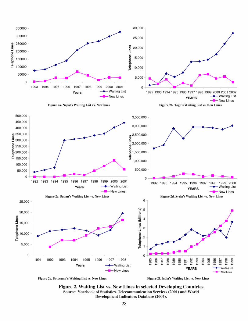
The historical behavior of demand and supply of telecommunications in

developing countries is shown in Figure 2. This behavior represents the supply problem

26

of telephone lines in developing countries, where the waiting list of subscribers are

higher than the new telephone lines available to connect (Pahlavan and Krishnamurthy,

2002). The waiting list of subscribers is part of the unmet or unsatisfied demand, which

is increased as more customers decide to subscribe to the telephone service. This

decision is based on the value the telephone service represents to the potential customer,

who considers the price and the usefulness of the service in order to make a decision.

On the other hand, the size of the waiting lists is decreased as more new telephones are

available. In developing countries, the number of new telephones deployed is a function

of the financial resources available and not of the unmet demand.

The problem of supply and demand of telephone lines in Nepal, Togo, Sudan,

Syria, Botswana, and India is shown in Figure 2, which shows the growth of waiting

lists and new telephones installed through time. It can be seen that the waiting lists are

growing and are higher than the new telephones lines connected per year. The statistics

do not consider the fact that unrecorded demand has beenwas found to be

approximately three times the number of orders in the waiting list (Wellenius, 1969). It

can also be observed that the gap between the waiting list and the new telephone lines is

also growing in several countries, such as the case of Nepal, Togo, Sudan, and Syria.

For instance, the waiting lists in Nepal grew from about 50,000 telephones in 1993 to

350,000 in 2001. However, the new telephones installed remained below 50,000 lines.

In the same manner, the waiting lists in Sudan grew from 50,000 telephones in 1992 to

450,000 telephones in 2001, and the new telephones installed remained below 100,000

lines. Additional data from several developing countries also confirm this behavior,

27

where the unmet applications (waiting lists) are even higher than the total supply of

telephone lines, which includes the total telephone lines installed and the new telephone

lines available to connect (Saunders et. al., 1994).

a) Africa b) Asia

c) Latin America

Figure 1. Telephones per 100 inhabitants Source: World Telecommunications Indicators Database (2004)

0123456789

1993 1994 1995 1996 1997 1998 1999 2000 2001 2002

Years

ZambiaMalaw iChadUgandaTogoBotswana

0123456789

1993 1994 1995 1996 1997 1998 1999 2000 2001 2002Years

NepalKyrgyzstanIndiaTurkmenistanTajikistan

0

2

4

6

8

10

12

1993 1994 1995 1996 1997 1998 1999 2000 2001 2002Years

El SalvadorBoliviaEcuadorHonduras

28

0

5,000

10,000

15,000

20,000

25,000

30,000

1992 1993 1994 1995 1996 1997 1998 1999 2000 2001 2002YEARS

Tele

phon

e Li

nes

Waiting ListNew Lines

0

50,000

100,000

150,000

200,000

250,000

300,000

350,000

400,000

450,000

500,000

1992 1993 1994 1995 1996 1997 1998 1999 2000 2001Years

Tele

phon

e Li

nes


0

500,000

1,000,000

1,500,000

2,000,000

2,500,000

3,000,000

3,500,000

1992 1993 1994 1995 1996 1997 1998 1999 2000YEARS

Tele

phon

e Li

nes


0

5,000

10,000

15,000

20,000

25,000

1991 1992 1993 1994 1995 1996 1997 1998Years

Tele

phon

e Li

nes

Wating ListNew Lines

0

1

2

3

4

5

6

1985

1986

1987

1988

1989

1990

1991

1992

1993

1994

1995

1996

1997

1998

1999

YEARS

Tele

phon

e Li

nes

(Mill

ions

)


Figure 2a. Nepal's Waiting List vs. New lines Figure 2b. Togo’s Waiting List vs. New Lines

Figure 2c. Sudan’s Waiting List vs. New Lines Figure 2d. Syria’s Waiting List vs. New Lines

Figure 2e. Botswana’s Waiting List vs. New Lines Figure 2f. India’s Waiting List vs. New Lines

Figure 2. Waiting List vs. New Lines in selected Developing Countries Source: Yearbook of Statistics. Telecommunication Services (2001) and World

Development Indicators Database (2004).

0

50000

100000

150000

200000

250000

300000

350000

1993 1994 1995 1996 1997 1998 1999 2000 2001Years

Tele

phon

e Li

nes


29

2.2 Regional Telephone Gap in Developing Countries

The growth of telephone lines in developing nations has been historically higher

in the urban areas, with respect to the rural areas (Saunders et. al., 1994). The data from

several developing countries provided by the ITU and other regulatory and statistical

entities of developing countries support this trend between urban and rural telephone

lines (Yearbook of Statistics. Telecommunications Services, 2001; World

Telecommunications Indicators Database, 2004; OSIPTEL of Peru; Superintendencia

de Telecomunicaciones of Bolivia; Department of Telecommunications of India; and

Bangladesh Bureau of Statistics).

Figure 3 shows the telephone density gap between rural and urban areas in

several developing countries of Africa, Asia, and Latin America. This figure shows the

ratio between rural and urban telephone densities. It can be seen that this ratio is less

than 0.3 in all three continents, which indicates that the telephone densities in the urban

areas are higher than three times the telephone densities in the rural areas. In most

cases, this ratio is decreasing, which shows that the telephone densities in the urban

areas are increasing faster than in the rural ones. This situation leads to an increase in

the regional telephone gap in developing countries through time.

The regional telephone density gap of Zambia, Malawi, Chad, Uganda, Togo,

and Botswana, which are developing countries from Africa, are shown in Figure 3. The

ratio between rural and urban telephone densities is less than 0.3 for all these countries,

which means that telephone densities in urban areas are higher than three times the

telephone densities in rural areas. In addition, it can also be seen that this ratio is

30

decreasing for Botswana, Chad, Malawi, and Uganda, which indicates the worsening of

the rural-urban telephone gap through time for these countries. The rural-urban

telephone density ratios for Nepal, Kyrgyzstan, India, Turkmenistan, and Tajikistan,

which are Asian developing countries, are also observed in this figure. It can be seen

that this ratio is less than 0.2 for all these countries, which indicates that telephone

densities in urban areas are higher than five times the telephone densities in rural areas.

In addition, it can also be seen that the rural-urban telephone gap is also getting worse

for India, Turkmenistan, and Tajikistan, since their rural-urban telephone density ratios

are also decreasing through time. The same behavior is also observed in Figure 3 for El

Salvador, Bolivia, Ecuador, and Honduras, which are developing countries from Latin

America. The rural-urban telephone density ratios are also less than 0.3 and are

decreasing for El Salvador, Bolivia, and Ecuador.

The higher dispersion of telephones in urban areas has been attributed to the

higher income per capita of the urban population, and the lower implementation costs

than the rural case, which restricts the telecom operator investment in more profitable

urban areas (World Bank, 2002). Previous research has found that income is the most

important variable that influences both demand of telephone lines and telephone traffic

(Saunders et. al., 1994). The income per capita in urban regions is higher than the

income per capita in rural areas. Therefore, the telephone traffic generated per

subscriber in rural areas is lower than it is in urban areas (Hudson, 1984).

31

a) Africa b) Asia

c) Latin America

Figure 3. The Rural-Urban Telephone Density Gap

Source: Estimated from World Telecommunications Indicators Database (2004) and World Development Indicators (2002)

0

0.05

0.1

0.15

0.2

0.25

0.3

1993 1994 1995 1996 1997 1998 1999 2000 2001 2002Years

ZambiaMalawiChadUgandaTogoBotswana

0

0.05

0.1

0.15

0.2

1993 1994 1995 1996 1997 1998 1999 2000 2001 2002Years

NepalKyrgyzstanIndiaTurkmenistanTajikistan

0

0.05

0.1

0.15

0.2

0.25

0.3

1993 1994 1995 1996 1997 1998 1999 2000 2001 2002Years

El SalvadorBoliviaEcuadorHonduras

32

2.3 Unsuccessful Telecommunications Policies in Developing Countries

The World Trade Organization (WTO) agreement of 1997 established

international commitments in the telecom sector for its country members. This implied

the transformation of the telecom law and regulations in order to align the country

objectives for the telecom sector with the international ones. Among the main policies

suggested by this agreement are the implementation of universal service, the autonomy

of the telecom regulator, free market for telecom services, and reduction of regulation

(The Telecommunications Development Bureau of ITU and CITEL, 2000).

The achievement of universal service indicated in the WTO agreement involves

the development of telecom infrastructure in rural areas of developing countries.

Universal service can be defined by the provision of “universal” availability of

connections to individual households from public telecommunication networks, with

non-discriminatory and affordable prices (Hank and McCarthy, 2000). An alternative to

universal service is “universal access”, which is defined by a situation where every

person has a reasonable means of access to a publicly available telephone. In practice,

progress toward universal service has been measured by the percentage of households

with telephone service (Cain and Macdonald, 1991).

Several policies and strategies have been implemented in the past by many

governments and institutions without success in order to solve the problem of universal

service in telecommunications (Malecki, 2003; Melody, 1999; Strover, 2003). Among

the most important policies are the privatization and liberalization of the telecom

33

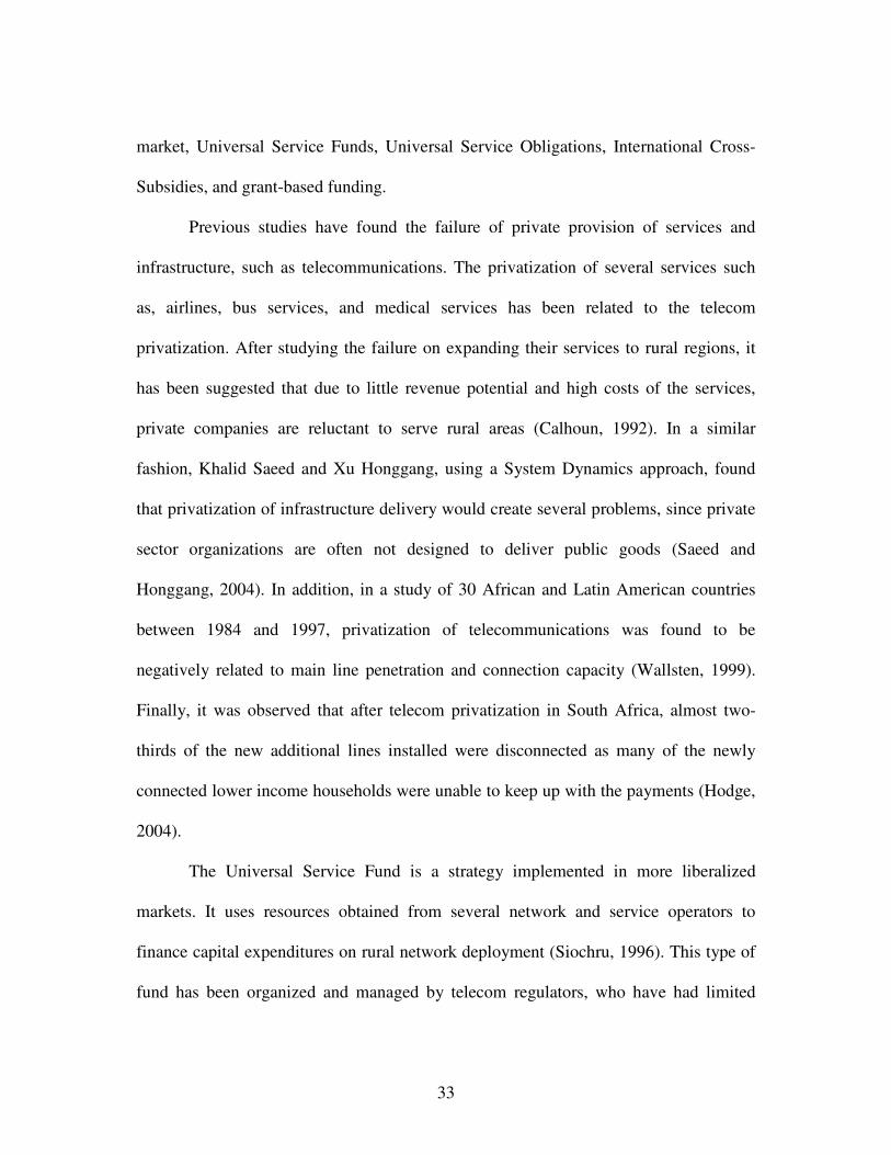
market, Universal Service Funds, Universal Service Obligations, International Cross-

Subsidies, and grant-based funding.

Previous studies have found the failure of private provision of services and

infrastructure, such as telecommunications. The privatization of several services such

as, airlines, bus services, and medical services has been related to the telecom

privatization. After studying the failure on expanding their services to rural regions, it

has been suggested that due to little revenue potential and high costs of the services,

private companies are reluctant to serve rural areas (Calhoun, 1992). In a similar

fashion, Khalid Saeed and Xu Honggang, using a System Dynamics approach, found

that privatization of infrastructure delivery would create several problems, since private

sector organizations are often not designed to deliver public goods (Saeed and

Honggang, 2004). In addition, in a study of 30 African and Latin American countries

between 1984 and 1997, privatization of telecommunications was found to be

negatively related to main line penetration and connection capacity (Wallsten, 1999).

Finally, it was observed that after telecom privatization in South Africa, almost two-

thirds of the new additional lines installed were disconnected as many of the newly

connected lower income households were unable to keep up with the payments (Hodge,

2004).

The Universal Service Fund is a strategy implemented in more liberalized

markets. It uses resources obtained from several network and service operators to

finance capital expenditures on rural network deployment (Siochru, 1996). This type of

fund has been organized and managed by telecom regulators, who have had limited

34

success in adapting the universal service goal to a competitive environment. The

management of the fund has been difficult due to problems in accurately measuring the

costs of universal service provision, and setting up funding mechanisms that are

efficient, equitable and that distort the market as little as possible (Duckworth, 2004).

For instance, in Ecuador, CONATEL, the Ecuadorian telecom regulator, was unable to

raise enough economic resources to finance significant telecom projects for the rural

areas, and reduce the gap in telecom infrastructure between rural and urban regions of

the country (Finance, Private Sector, and Infrastructure Development of World Bank,

2001). In Ghana, the government plans to charge all operators a tax to create a fund for

rural development but the fund still does not exist. In Ivory Coast, the fund exists but

has not yet been used (Laffont and N’Gbo, 2000).

Finally, the grant-based funding uses resources from the general budget to

subsidize the deployment of telecom infrastructure (Kayani and Dymond, 1997). This

strategy was found to improve considerably telecom penetration in developing countries

(Ramos and Gerstenfeld, 2004), although it uses scarce economic resources that are

generally unavailable for telecommunications investment. In addition, there are still

several questions regarding the sustainability of the implementations, since there have

been cases where the expansion of telecom infrastructure did not translate into

sustainable projects. For instance, a rural telecom company from Chile, which has been

subsidized by the government for implementing rural telecom projects, has been losing

money (Wellenius, 2002).

35

2.4 Universal Service Obligations and International Cross-Subsidies

The principles dictated by welfare economics say that the price of each product

or service should be set equal to its marginal cost, and output should be expanded to

meet resulting demand at those prices. In this context, there should not be cross-

subsidization, whereby one service is priced above marginal cost to finance the supply

of a service at a price below marginal cost (Littlechild, 1979).

On the other hand, the cross-subsidies in telecommunications have been

regarded as a useful mechanism for expanding networks in rural and poor areas of

developing countries (Laffont and N’Gbo, 2000), even in the presence of competition

(Gasmi et al., 2000). It has been proposed that cross-subsidizations through the

provision of telecommunications at prices below cost may sometimes be desirable in

order to spread the benefits of telecom access to disadvantaged and rural remote areas,

where the cost of providing access is generally higher than in urban areas, the total

traffic generated is relatively low, and the telecom income from the service provision is

also low (Saunders et. al., 1994; The Telecommunications Development Bureau of ITU,

and CITEL, 2000). These cross-subsidizations are supposed to create positive network,

call, and social externalities, which should improve rural development and social

efficiency and benefit (Crandall and Waverman, 2000; Saunders et al., 1994). The

question addressed in this investigation is whether the intended improvement will

actually happen in the long term given that there exist differences in income per capita

and willingness to pay, telephone deployment and operating costs, and telephone

deployment delays in urban and rural areas.

36

In several developing countries, cross-subsidization has been applied by

overcharging for international long distance and providing local access below cost, and

by applying Universal Service Obligations fees to telecom investment in less profitable

rural areas (Kayani and Dymond, 1997). These cross-subsidization policies have been

implemented in the past with the objective of increasing telephone density and

promoting universal service in telecommunications. Universal service in

telecommunications is part of the World Trade Organization (WTO) agreement of 1997

and involves the development of telecom infrastructure in rural areas (The

Telecommunications Development Bureau of ITU, and CITEL, 2000).

These types of subsidies are typical for telephone services that are regulated and

mandated by the government to provide an affordable and accessible service, such as

the case of the fixed ‘wired’ telephone service in most developing countries. On the

other hand, the cellular telephone service, which is less regulated or more liberalized, is

not significantly affected by these cross-subsidies. However, it was explained before

that private telecom providers do not prefer to extend the service to unprofitable rural

areas and are often not designed to deliver public goods (Calhoun, 1992; Madden et al.,

2004; Saeed and Honggang, 2004).

2.4.1 International Cross-Subsidies.

Traditionally the tariffs for telecom services have been based in political and

social objectives, including advancing universal service, the result is the generation of

cross-subsidies. These cross-subsidies can occur between different services, geographic

37

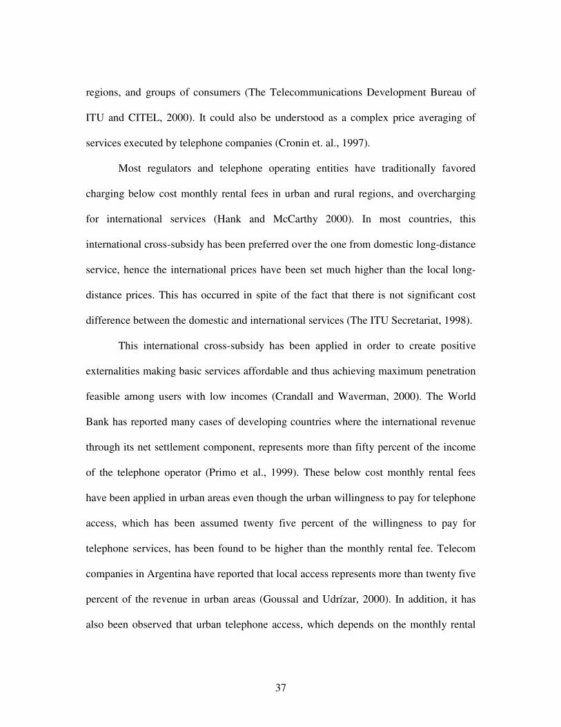
regions, and groups of consumers (The Telecommunications Development Bureau of

ITU and CITEL, 2000). It could also be understood as a complex price averaging of

services executed by telephone companies (Cronin et. al., 1997).

Most regulators and telephone operating entities have traditionally favored

charging below cost monthly rental fees in urban and rural regions, and overcharging

for international services (Hank and McCarthy 2000). In most countries, this

international cross-subsidy has been preferred over the one from domestic long-distance

service, hence the international prices have been set much higher than the local long-

distance prices. This has occurred in spite of the fact that there is not significant cost

difference between the domestic and international services (The ITU Secretariat, 1998).

This international cross-subsidy has been applied in order to create positive

externalities making basic services affordable and thus achieving maximum penetration

feasible among users with low incomes (Crandall and Waverman, 2000). The World

Bank has reported many cases of developing countries where the international revenue

through its net settlement component, represents more than fifty percent of the income

of the telephone operator (Primo et al., 1999). These below cost monthly rental fees

have been applied in urban areas even though the urban willingness to pay for telephone

access, which has been assumed twenty five percent of the willingness to pay for

telephone services, has been found to be higher than the monthly rental fee. Telecom

companies in Argentina have reported that local access represents more than twenty five

percent of the revenue in urban areas (Goussal and Udrízar, 2000). In addition, it has

also been observed that urban telephone access, which depends on the monthly rental

38

fee, is considerably inelastic when compared with rural areas (GAS 5 Economic Studies

at the National Level in the Field of Telecommunications, 1984; Goussal and Udrízar,

2000).

The international cross-subsidy obligates operators to use funds obtained from

international calls, to invest in the expansion of the urban and rural telecom network

while maintaining the local prices and fees at low values in order to increase demand

and telecom penetration. The common rationality of cross-subsidization is that users

cannot afford to pay the full cost-based fee for service due to high costs involved in its

implementation and operation (Kayani and Dymond, 1997). The provision of

telecommunications at prices below cost may sometimes be desirable in order to spread

the benefits of telecom access to smaller towns or rural remote areas, where the cost of

providing access is generally higher than it is in urban areas, the total traffic generated

is relatively low, and the telecom income from the service provision is also low

(Saunders et. al., 1994).

In developing countries, the urban and rural monthly rental fees have been held

down under the common rationality of pricing basic service below cost in order to

generate positive externalities and support the universal service policy. These

externalities include network, call, and social externalities, which are generated by the

action of one individual that benefits others without a corresponding payment, or

revenue flow, to the individual generating them (Crandall and Waverman, 2000).

Table 1 shows a list of countries that have applied cross-subsidization by

holding the monthly rental fee at considerably lower values than the operating costs and

39

at the same time overcharging for its international service. This situation is observed in

the ratio of operating costs per telephone line to monthly rental fee in urban areas and in

the cost of a 3-minute call to the United States from these developing countries. For

instance, the ratio of urban operating costs per line to the urban monthly rental fee in

Zambia is 20.25, which indicates that the operating costs per line are more than twenty

times higher than the monthly rental fee in urban areas. On the other hand, it can also be

observed that the international price of a 3-minute phone call from Zambia to the United

States is 2.57 dollars, which has been used to create the international cross-subsidy. In

the same manner, the operating costs per line in Botswana are thirty eight times higher

than monthly rental fee in urban areas, and the international price of a 3-minute phone

call from Botswana to the United States is 3.6 dollars. The operating costs per line in

Bolivia are twenty five times higher than the monthly rental fee in urban areas, and the

international price of a 3-minute phone call is 3.7 dollars.

It is also observed that monthly rental fee is much lower than the willingness to

pay for telephone access in urban areas, which indicates that local telephone access is

underpriced. This can be observed in the ratio of willingness to pay for telephone access

to monthly rental fee in urban areas. The ratio of urban willingness to pay for telephone

access to urban monthly rental fee in Botswana is 8.39, which indicates that access

willingness to pay is higher than eight times the monthly rental fee in urban areas.

Similarly, the access willingness to pay in Bolivia is higher than three times the

monthly rental fee in urban areas. In the same manner, the access willingness to pay in

Thailand is higher than fourteen times the monthly rental fee in the urban areas.

40

The willingness to pay for the telephone service has been defined as five percent

of the income per household (Hank and McCarthy, 2000; Kayani and Dymond, 1997),

since the International Telecommunications Union (ITU) has determined that household

expenditure in telecommunications could be up to five percent of the income (Milne,

2003). The operating cost has been defined as thirty percent of the capital costs, which

is the world average. The cost per line is defined as a function of the cable distance,

which is a function of the population density (Kayani and Dymond, 1997; Calhoun,

1992; Webb, 2000).

The capital costs per line depend on the average cable distance from the central

office to the subscribers (Kayani and Dymond, 1997). It is defined as a function of the

population density and a referential number of telephone lines per central office, which

is assumed five thousand. As a reference, the cost of a telephone line in urban areas of

Ecuador has been previously estimated below five hundred dollars (Plaza, 2005). The

urban income per capita is defined as a function of the non-agricultural income and the

urban population density depends on the urban area, which it assumes represents ten

percent of the land area (Kayani and Dymond, 1997).

41

Table 1. International Cross-Subsidies in selected Developing Market Economies.

Source: World Telecommunications Development Report (2001). Data estimated from: World

Telecommunications Indicators Database (2004), World Development Indicators (2002)

2.4.2 Universal Service Obligations

Governments and regulatory authorities have created Universal Service

Obligations to generate positive network, call, and social externalities and guarantee

service above a certain threshold to rural areas, which are intended to accelerate rural

development and to improve the social efficiency in developing countries. The

Universal Service Obligations give priority to investment into rural areas, which usually

go beyond the feasible cost/revenue limits and require cross-subsidization from more

profitable urban regions and services (Kayani and Dymond, 1997). These obligations

have been applied by increasing the investment in rural telecom capacity, even though

there is evidence of higher operating costs and lower willingness to pay in rural areas

with respect to urban areas. This process is expected to result in a faster expansion of

Urban Urban Monthly Urban Urban Urban Urban Op. Cost / Cost of CallCountry Income Access Rental Acess Population Cost per Operating Mo. Fee to US $ per

per Capita Willingness Fee W. to Pay / Density Line Costs Ratio 3 minutes(US to Pay (US Mo. Fee (US (US

dollars) (US dollars) dollars) Ratio (pop/km2) dollars) dollars) (year 2000)Zambia 498 2.07 1.14 1.82 58 921 23.02 20.25 2.57Bolivia 1230 5.13 1.62 3.17 47 1003 25.07 15.50 3.7Ecuador 1708 7.12 6.20 1.15 284 515 12.87 2.07 4.9Honduras 1599 6.67 2.43 2.74 252 535 13.39 5.50 4.2Thailand 8155 33.98 2.33 14.60 262 529 13.21 5.68 2.5Botswana 5088 21.20 2.53 8.39 17 1548 38.71 15.31 3.6Colombia 2329 9.70 2.68 3.62 277 519 12.97 4.84 2.2

42

rural telecom infrastructure, but it is achieved at the expense of limiting service to urban

and high-density areas (Goussal and Udrízar, 2000).

Table 2 shows a list of countries that have applied Universal Service

Obligations, even though the ratio of willingness to pay to operating cost per line is

much higher in urban areas with respect to rural areas. The ratio of willingness to pay to

operating costs per line in the urban areas of Botswana is 0.88. This ratio is much higher

than 0.01, which is the ratio of willingness to pay to operating costs per line in the rural

areas. This shows the higher willingness to pay for telephone services and lower

operating costs per line in the urban areas with respect to the rural areas in Botswana.

Similarly, in Honduras, the ratio of willingness to pay for telephone services to

operating costs per line in urban areas is 0.8, which is much higher than 0.07, the ratio

of willingness to pay to operating costs per line in the rural areas. In the same manner,

the ratio of willingness to pay for telephone services to the operating costs per line in

the urban areas of Nepal is 0.55, which is much higher than 0.05, the ratio of

willingness to pay for telephone services to operating costs per line in the rural areas.

As indicated before, this shows the higher willingness to pay for telephone services and

lower operating costs per line in the urban areas with respect to the rural areas in Nepal.

It is also observed that the willingness to pay is higher in urban areas because of

the higher incomes per capita in these regions. The willingness to pay for telephone

services in the urban areas of Bangladesh is eight dollars, which is much higher than

one dollar, the willingness to pay for telephone services in the rural areas. This is

proportional to the income per capita of the urban and rural population in Bangladesh.

43

The income per capita in the urban areas of Bangladesh is 1,143 dollars and the income

per capita in the rural areas is 120 dollars. Similarly, the willingness to pay for

telephone services and the income per capita of the urban population in Honduras is 11

dollars and 1,599 dollars respectively. On the other hand, the willingness to pay for

telephone services and the income per capita of the rural population in Honduras is 2

dollars and 311 dollars respectively.

The operating costs are found to be higher in rural areas because of the lower

population densities, which increase the cost of a telephone line and the capital costs.

For instance, the rural operating costs in Ecuador are much higher than the urban

operating costs. The rural population density of Ecuador is 19 people per square

kilometer and the rural operating cost per line is thirty-seven dollars per month. On the

other hand, the urban operating cost per line in Ecuador is thirteen dollars per month

and its urban population density is 284 people per square kilometer. Similarly, the urban

operating cost per line in Bolivia is twenty-five dollars per month, which is much lower

than eighty-eight dollars per month, the rural operating cost per line. These values are

inversely proportional to the urban and rural population densities. The Bolivian urban

population density is 47 people per square kilometer and its rural population density is 3

people per square kilometer.

Table 3 shows details of the application of Universal Service Obligations in

selected developing countries from Asia, Africa, and South America. Several countries

in Asia have adopted Universal Service Obligations in order to expand rural

telecommunications. The government of India created the “Universal Service

44

Obligation”, which requires the installation of ten percent of their total installed

capacity in rural areas from all telecom operators (Hank and McCarthy, 2000; Peha,

1999). In Nepal, the telecom regulatory authority mandates telecom operators to

provide rural telecommunications in the entire country (Nepal Telecommunications

Authority, 2004). The license of the telecom operator in Bangladesh obliges the

installation of one exchange in each sub-District or Thana. In Pakistan, the telecom

operator was mandated to install 150,000 new telephone lines in rural areas to reach

villages with over 1,000 inhabitants and achieve a rural telephone density of 0.2 lines

per 100 inhabitants by 1998. In Thailand, the government mandated the expansion of

the telephone service to cover all villages with 2 lines in each sub-village (Kayani and

Dymond, 1997).

Africa seems to follow in the footsteps of Asia regarding the implementation of

Universal Service Obligations. The government of Botswana mandated the state-owned

telecom company to serve all identifiable demand in villages with a population higher

than five hundred by the year 2000 (Kayani and Dymond, 1997). The government of

Togo recently mandated the extension of rural telecommunications by providing a

telephone within a distance of less than 5 km by 2010 (The Sun News On-Line, 2004).

In Latin America several countries have implemented Universal Service

Obligations either in their national programs or as part of the carrier’s license

agreement. The privatized telecom company in Bolivia, ENTEL, has spent forty percent

of its expansion budget on rural areas. The government of Honduras has a telecom

Rural Master Plan, which gives rural areas priorities for investment. The telecom

45

operators in Ecuador are mandated to deploy rural telecommunications as part of their

license agreement (Kayani and Dymond, 1997).

Table 2. Indicators of Selected Developing Market Economies with Universal

Service Obligations

Source: Data estimated from World Development Indicators (2002)

CountryUrban Rural Urban Rural Urban Rural Urban Rural Urban Rural

Togo 488 147 8 2 289 65 13 22 0.64 0.11Nepal 1217 111 20 2 188 153 15 16 1.37 0.12India 1199 155 20 3 865 247 9 13 2.15 0.19Bangladesh 1143 120 19 2 2183 768 8 10 2.53 0.21Pakistan 884 182 15 3 641 121 10 17 1.46 0.18Bolivia 1230 644 21 11 47 3 25 88 0.82 0.12Ecuador 1708 310 28 5 284 19 13 37 2.21 0.14Honduras 1599 311 27 5 252 32 13 30 1.99 0.18Thailand 8155 256 136 4 262 103 13 18 10.28 0.23Botswana 5088 212 85 4 17 2 39 107 2.20 0.03

(dollars) (pop/Km2)

Operating

(dollars)

Willingness toIncomeper Capita Pay Density Cost

Willingness to Pay /Population

(dollars)Operating Costs

46

Country UNIVERSAL SERVICE OBLIGATION

Togo The government of Togo recently mandated the extension of rural telecommunications

by providing a telephone within a distance of less than 5 km by 2010.

Nepal The telecom operators are obliged to make a contribution to the rural

telecommunications fund annually for rural telecom projects.

India It demanded the installation of ten percent of their total installed capacity in rural areas.

Bangladesh The license of operation obliged the installation of one exchange in each sub-District

(Thana)

Pakistan The installation of 150,000 new telephone lines in rural areas to reach villages with over

1,000 inhabitants and achieve a rural telephone density of 0.2 lines per 100 inhabitants

by 1998.

Bolivia The privatized telecom company ENTEL spends 40% of its expansion budget on rural.

Ecuador Rural telecommunications is part of the operation license of the telecom operators

Honduras The country has a telecom Rural Master Plan, which gives rural areas priorities of

investment.

Thailand The expansion of telephone service to cover all villages with 2 lines in each sub-village.

Botswana The government mandated the telecom operator to serve all villages with a population

higher than five hundred people.

Table 3. Universal Service Obligation Policies in selected Developing Market

Economies.

Source: Kayani and Dymond (1997), Peha (1999), The Sun News On-Line (2004), Nepal

Telecommunications Authority (1994)

47

2.5 Performance of Universal Service Obligations and International Cross-

Subsidies in Developing Countries.

Table 4 shows that the International Cross-Subsidies applied in developing

countries had little effect on improving the dispersion of telephone services. For

instance, in Zambia the overall as well as urban and rural telephone densities were

reduced, in spite of the application of the Internal Cross-Subsidy indicated in Table 1.

The monthly rental fee in Zambia is about twenty times less than the operating cost, and

two times lower than the willingness to pay for telephone access in urban areas. The

below cost monthly rental fee is implemented by charging high prices for international

traffic. In the same manner, in Bolivia and Colombia the telephone densities

experienced little improvement and the rural telephone densities were reduced. This

increased the telephone gap between urban and rural regions, in spite of implementing

monthly rental fees that are much lower than the urban operating costs and the

willingness to pay for telephone access.

The application of Universal Service Obligations has also done little to improve

the telephone density and especially the penetration of rural telephone lines in other

developing countries, as observed in Table 4. For instance, in Bangladesh the

penetration of telephone lines in rural areas grew from 0.03 lines per 100 inhabitants in

1993 to 0.05 lines per 100 inhabitants in 2002, which did not reduce the service gap

between urban and rural regions. In Bolivia and Ecuador the overall telephone densities

had little improvement and the rural telephone densities were reduced. This increased

48

the urban-rural telephone gap and occurred in spite of the application of the USO

policies described in Table 3.

The model developed in this dissertation investigates if the society is going to

benefit by overcharging for international services and charging monthly rental fees

below cost, and by applying Universal Service Obligations in terms of achieving higher

telephone densities and reducing the rural-urban telephone gap.

Table 4. The Dispersion of Telephones in Selected Developing Market Economies

with USO and International Cross-Subsidies.

Source: World Telecommunications Indicators Database (2004), Kayani and Dymond (1997), Peha

(1999), The Sun News On-Line (2004), Nepal Telecommunications Authority (2004). Data estimated

from World Development Indicators (2002).

Countries1993 2002 1993 2002 1993 2002 1993 2002 1993 2002 USO INT

Zambia 0.92 0.81 1.89 1.70 0.30 0.24 20 18 0.160 0.140 �

Togo 0.45 1.05 1.59 3.12 0.01 0.08 1 5 0.004 0.025 �

Nepal 0.37 1.41 4.07 12.69 0.00 0.02 1 1 0.001 0.001 �

India 0.89 3.98 3.20 10.38 0.12 1.49 10 27 0.037 0.144 �

Bangladesh 0.21 0.46 0.99 1.84 0.03 0.05 10 8 0.026 0.026 �

Pakistan 1.24 2.5 3.68 6.25 0.09 0.39 5 10 0.025 0.063 �

Low Income 0.68 1.70 2.57 6.00 0.09 0.38 8 12 0.042 0.066 5 1Bolivia 3.28 6.37 5.39 10.23 0.60 0.33 8 2 0.111 0.032 � �

Ecuador 5.45 11.02 8.92 16.97 1.21 0.89 10 3 0.136 0.053 � �

Honduras 2.1 4.81 4.45 7.83 0.40 1.67 11 17 0.090 0.213 � �

Thailand 3.93 10.5 13.24 27.00 1.75 6.11 36 46 0.132 0.226 � �

Botswana 3.12 8.28 5.86 13.18 1.22 3.57 23 22 0.208 0.271 � �

Colombia 8.46 17.94 8.95 24.08 7.37 1.33 27 2 0.823 0.055 �

Middle Income 4.39 9.82 7.80 16.55 2.09 2.32 19 15 0.250 0.142 5 6

Rural Telep. DensityTelephone Density Urban Telep. DensityLines per 100 Inhab Lines per 100 Inhab Lines per 100 Inhab Lines

Rural/Urban Telecom % RuralTelep. Density Gap Policies

49

Chapter 3 Methods of Analysis for Telecom Planning and Policies

3.1 The Failure of Current Methods for Telecom Planning and Policy Design.

The current policies and strategies for increasing telecommunications

deployment in rural areas are often insufficient or unsuccessful, and the plans for

expansion of local telephone networks are generally imprecise considering the scope of

the investment (Malecki, 2003; Melody, 1999; Strover, 2003; Calhoun, 1992). The

telecom gap between urban and rural regions and between the rich and poor people has

not improved using current policies and strategies (Saunders et. al., 1994; Kayani and

Dymond, 1997; Malecki, 2003; Cain and Macdonald, 1991). In addition, conventional

management rationality such as the ‘Get Big Fast’ strategy triggered the biggest crises

of the telecom industry: the Internet stock bubble in the late 1990s and the ‘dot.com’

crash of business to consumer (B2C) electronic commerce companies of the year 2000

(Oliva et. al., 2002)

One of the conventional methods used for telecom planning and policy design is

the use of econometric modeling. This uses statistical methods to verify and quantify

economic theory, which relies on statistical verification of model structure and

parameters by tying the models firmly to statistical observations of real world systems.

The econometric analysis uses correlated rather than directly causally related variables

to proceed in spite of the empirical validation requirement (Meadows, 1980).

The econometric modeling requires representing economic systems as linear,

which allows the mathematical estimation of parameters; and includes fudge factors to

50

the output of a model with the purpose of fitting modeler’s intuition (Sterman, 2000).

There is a problem related to the different estimation techniques used in econometric

analyses, it has led to different conclusions about the effects of specific telecom policies

in developing countries (Fink et. al., 2003). For instance, there are different conclusions

about the impact of telecom privatization using econometric modeling. Wallsten found

in a study of 30 African and Latin American countries between 1984 and 1997, that

privatization of telecommunications was negatively related to main line penetration and

connection capacity, and Ros and Banerjee found that telecom privatization is good for

telecom expansion (Wallsten, 1999; Ros and Banerjee, 2000). In addition,

counterproductive telecom policies could be derived as a result of the application of this

methodology. Saeed and Honggang have proved that privation of public telephone

services might not be good for telephone dispersion and achieving universal service in

telecommunications ( Saeed and Honggang, 2004).

The survey analysis for collecting and analyzing data is another common

conventional methodology for telecom planning and policy design. This methodology

requires designing questionnaires and distributing them over a target population, in

order to gather information, such as the experiences, knowledge, opinions, or

perceptions, from the main stakeholders of the system. The problems found in this

methodology are related to the design of the questionnaires, which could be biased or

poorly elaborated, and to the population surveyed, which could not be big enough or

representative of the problem being studied. In addition, it relies on the limited

rationality, and understanding of the problems related to the complex telecom system,

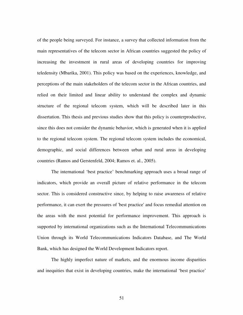
51

of the people being surveyed. For instance, a survey that collected information from the

main representatives of the telecom sector in African countries suggested the policy of

increasing the investment in rural areas of developing countries for improving

teledensity (Mbarika, 2001). This policy was based on the experiences, knowledge, and

perceptions of the main stakeholders of the telecom sector in the African countries, and

relied on their limited and linear ability to understand the complex and dynamic

structure of the regional telecom system, which will be described later in this

dissertation. This thesis and previous studies show that this policy is counterproductive,

since this does not consider the dynamic behavior, which is generated when it is applied

to the regional telecom system. The regional telecom system includes the economical,

demographic, and social differences between urban and rural areas in developing

countries (Ramos and Gerstenfeld, 2004; Ramos et. al., 2005).

The international ‘best practice’ benchmarking approach uses a broad range of

indicators, which provide an overall picture of relative performance in the telecom

sector. This is considered constructive since, by helping to raise awareness of relative

performance, it can exert the pressures of 'best practice' and focus remedial attention on

the areas with the most potential for performance improvement. This approach is

supported by international organizations such as the International Telecommunications

Union through its World Telecommunications Indicators Database, and The World

Bank, which has designed the World Development Indicators report.

The highly imperfect nature of markets, and the enormous income disparities

and inequities that exist in developing countries, make the international ‘best practice’

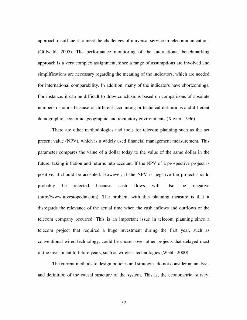
52

approach insufficient to meet the challenges of universal service in telecommunications

(Gillwald, 2005). The performance monitoring of the international benchmarking

approach is a very complex assignment, since a range of assumptions are involved and

simplifications are necessary regarding the meaning of the indicators, which are needed

for international comparability. In addition, many of the indicators have shortcomings.

For instance, it can be difficult to draw conclusions based on comparisons of absolute

numbers or ratios because of different accounting or technical definitions and different

demographic, economic, geographic and regulatory environments (Xavier, 1996).

There are other methodologies and tools for telecom planning such as the net

present value (NPV), which is a widely used financial management measurement. This

parameter compares the value of a dollar today to the value of the same dollar in the

future, taking inflation and returns into account. If the NPV of a prospective project is

positive, it should be accepted. However, if the NPV is negative the project should

probably be rejected because cash flows will also be negative

(http://www.investopedia.com). The problem with this planning measure is that it

disregards the relevance of the actual time when the cash inflows and outflows of the

telecom company occurred. This is an important issue in telecom planning since a

telecom project that required a huge investment during the first year, such as

conventional wired technology, could be chosen over other projects that delayed most

of the investment to future years, such as wireless technologies (Webb, 2000).

The current methods to design policies and strategies do not consider an analysis

and definition of the causal structure of the system. This is, the econometric, survey,

53

international benchmarking, and net present value analysis do not consider the structure

of the regional telecom system for policy and strategy design. In addition, the use of

microeconomic theory and the ‘future scenario’ technique do not involve the study of

the dynamic relationships between the different elements of the telecom system either.

The ‘future scenario’ technique has been used to anticipate customer expectations,

economical constraints, and potential business models for telecom operators, which

considers current trends in science and technology in order to project likely images of

future societies (Unbehaun, 2002; Flament et. al., 1999)

3.2 System Dynamics as a Methodology for Policy Design and Planning of Rural

Telecommunications.

The previous section described some clear problems related to the conventional

methodologies used for telecom planning and evidenced the need of a more effective

and appropriate methodology. The need for a systems framework to analyze the

complexity of the rural telecommunication system and the importance of focusing on

economic and social aspects rather than only the technological ones has been

recognized to some degree (Andrew and Petkov, 2003). In addition, the importance of a

procedure for rural telecom planning that can react to changing circumstances in a

dynamic manner has been previously supported (Walsham, 1979), and a systematic

investigation of the determinants of diffusion of mobile telecommunications, which

could be used for rural telecommunications, has been previously recommended (Gruber,

2001). The adoption of new modeling practices for the telecommunications industry,

54

which can incorporate the trade-offs raised by the emergence of wireless access

alternatives, especially when applied to rural environments, has been suggested

(Calhoun, 1992).

Telecom planning using a long-term and non-linear system dynamics approach

as compared to ‘tactical’ approaches, which are reactive, short-term, and linear, has

been advocated (Lyneis, 1994). The definition of the dynamic hypothesis in the system

dynamics methodology determines the structure of the regional telecom system, which

incorporates the social, economic, and demographic variables of the urban and rural

areas and the interrelationships between them. For instance, this incorporates variables

such as, the willingness to pay for telephone services and the income per capita of the

urban and rural population, and the population densities and operating costs of the

telecom network, and relationships such as, the connecting rate of telephones is a

function of the telephone capacity. Computer simulation performed through system

dynamics allows inferring future long-term behavior, as a result of the dynamic

interaction of the different elements of the regional telecom system. The future behavior

could be exponential or linear growth, oscillation, S-shaped growth, overshoot and

collapse, goal seeking, and growth with overshoot. Once the regional telecom system

has been built, the physical variables and the actual relationships of the system facilitate

the design of new policies for improving the behavior of the regional telecom system,

such as improving the number of telephone lines in rural areas of developing countries.

The chance of implementation of new telecom policies, which have been designed by

55

system dynamics modeling, is relatively high, since the policies consider the actual real

variables of the regional telecom system.

As in every industry, telecommunications is composed of markets,

organizations, regulations, resources, and technologies. The relationships between these

entities is not static, there is a dynamic interaction which demands a dynamic analysis.

The analysis of the interactions between different elements of the telecommunications

industry can be appropriately done by the use of system dynamics. Jay Forrester in his

book ‘Industrial Dynamics’ showed how different elements of an industry are modeled

as a set of relationships and feedback loops. Jay Forrester also modeled the market

growth in a particular industry. System dynamics has already been used for modeling

the growth of the telecom market through establishing relationships between different

sectors of the telecom industry such as, demand and supply (Jensen et. al., 2002; Lyons

et. al., 1997; Bui and Loebbecke, 1996; Ramos and Gerstenfeld, 2004; Dutta and Roy,

2003).

The study of policy issues and regulatory aspects of telecommunications is

suitable to the use of system dynamics. System dynamics deals with the limitation of

bounded rationality or a linear cause-and-effect relationship commonly applied in

policy or strategy design and considers the main interactions between the different

elements of the telecom market. For this reason, SD has been widely used in the design

of policies and strategies in several fields. In fact, several papers and books have been

written where system dynamics has been used as the methodology for modeling policies

and strategies of corporations and nations (Saeed, 1994; Lyneis, 1980). The design of

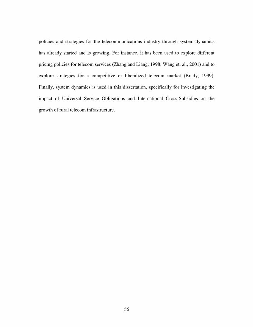
56

policies and strategies for the telecommunications industry through system dynamics

has already started and is growing. For instance, it has been used to explore different

pricing policies for telecom services (Zhang and Liang, 1998; Wang et. al., 2001) and to

explore strategies for a competitive or liberalized telecom market (Brady, 1999).

Finally, system dynamics is used in this dissertation, specifically for investigating the

impact of Universal Service Obligations and International Cross-Subsidies on the

growth of rural telecom infrastructure.

57

Chapter 4 Formulation of the Regional Telecommunications System

This model considers a case of government or privately owned telecom

monopoly, whose tariffs are fixed and regulated by the government. The

telecommunications in developing countries is still a monopoly in many senses, even

when competition is introduced. The international experience has shown that the

incumbent manages to retain its leadership position and market power long after

liberalization (Makhaya and Roberts, 2003). Many countries implement this model in

the public sector, but it is important to note that the implementation of Universal

Service Obligations and International Cross-Subsidies also happens in privatized

markets when mandated by telecom regulatory authorities.

The model is divided into 4 sectors: 1) Telephone Demand, 2) Telephone

Deployment, 3) Telephone Traffic, and 4) Financial Resources. These sectors are

replicated for two regions: urban and rural. At an aggregate level, the interactions

between the sectors can be represented by the causal diagram in Figure 4.

Telephone Demand represents the subscribers with telephone lines and the

unmet demand, which is composed of subscribers in the waiting list and potential

subscribers willing to pay the monthly rental fee but not decided to pay the activation

fee and the telephone device cost yet. The subscribers in the waiting list are connected

at a rate, which depends on the new telephone capacity. Telephone Deployment

represents the process of deployment of new telephone capacity, which is a function of

the amount of economic resources available, the number of subscribers in the waiting

list, the current number of new telephone lines ready to be connected, and the number

58

of telephone lines being deployed. Telephone Traffic represents the level of usage of the

telephone network in urban and rural areas as a function of the price, income per capita

of the population, and the current penetration of telephone lines in the region. Financial

Resources accumulates the economic resources used in the expansion of telecom

infrastructure in urban and rural areas. Financial Resources depends on the number of

subscribers, the telephone traffic, the price of the service, the operating costs, and the

amount of money invested in telecom infrastructure.

Each sector shown in Figure 4 represents the regional telecom system and is

driven by decision rules created by its own working environment while also reacting to

information and inputs received from other sectors. The structure of each sector and

detailed mathematical relationships of the model are discussed below.

59

Urban TelephoneDemand

Rural TelephoneDemand

FinancialResources

Rural Traffic

Urban Traffic

+

+

+

+Rural TelephoneDeployment

Urban TelephoneDeployment

+

+

+

+

+

+

+

-

+

-

Figure 4. A Simplified Sector Map of the Regional Telecom System.

60

4.1 Telephone Demand Sector

Figure 5. Telephone Demand Sector

The Telephone Demand sector shown in Figure 5 is represented as a supply

chain, both in rural and urban regions, where the population is the source of potential

customers; the potential customers become subscribers in the waiting list; and

subscribers in the waiting list become connected customers.

The actual demand of telephone lines includes connected customers, customers

in the waiting list, and potential customers. The population becomes potential

consumers when the utility of the service is higher than its price. The price represents

the monthly rental fee for the postpaid telephone service. The potential customers

become customers in the waiting list after they are willing to pay for the activation

charges and/or telephone devices (Warren, 2002). The customers in the waiting list

become connected subscribers when they get connected, which depends on the

connecting capacity of the telephone company (Jensen et. al., 2002). The connected

Potential Customers Waiting List Connected Subscribers

Rate of NewCustomers

Rate of ConnectingCustomers

New PotentialCustomers Rate

NetworkExternality Impact

Indicated Demand

Monthly RentalFee

DemandAdjustment

Activation and DeviceAcceptance Delay

Connecting Rate

Population

Demand Fraction

Actual Demand

Income perSubscriber

61

subscribers, therefore represent the part of the demand that can be served under the

current conditions of supply (Ros and Banerjee, 2000). The connected subscribers

create the revenue that feeds into the financial resources of the telephone company, as

shown in Figure 5.

Potential new customers adjust towards an indicated demand for new lines,

which is a function of the total population, the impact of telephone density as a network

externality factor, the monthly rental fee, and the income per subscriber. In addition, it

is assumed that the impact of telephone density on rural access demand is lower than

the impact on urban areas, which is borne out by evidence concerning the income and

preferences of the rural population in developing countries (Goussal and Udrízar, 2000;

GAS 5, 1984; Wellenius, 2002).

The impact of the monthly rental fee on indicated demand is determined by the

elasticity of the demand with respect to the monthly rental fee, which has been observed

to be higher in rural areas than in urban areas, because of the lower income levels and

perceived usefulness of the service (Cain and Macdonald, 1991).

4.2 Equations of the Telephone Demand Sector

It is assumed that the number of connected subscribers (CS) is increased by the

connecting rate (CR) and decreased by the connected customers attrition rate (AR). The

connecting rate (CR) is a function of the fraction of lines connected per month (FLC),

the postpaid-prepaid waiting list fraction (PPWLF), and the telephone capacity (TC),

which represents the telephone lines recently deployed and ready to be allocated to a

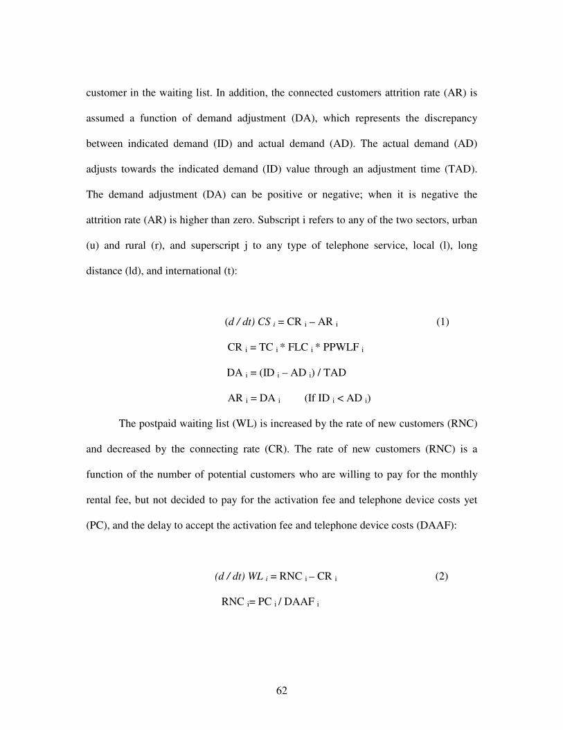
62

customer in the waiting list. In addition, the connected customers attrition rate (AR) is

assumed a function of demand adjustment (DA), which represents the discrepancy

between indicated demand (ID) and actual demand (AD). The actual demand (AD)

adjusts towards the indicated demand (ID) value through an adjustment time (TAD).

The demand adjustment (DA) can be positive or negative; when it is negative the

attrition rate (AR) is higher than zero. Subscript i refers to any of the two sectors, urban

(u) and rural (r), and superscript j to any type of telephone service, local (l), long

distance (ld), and international (t):

(d / dt) CS i = CR i – AR i (1)

CR i = TC i * FLC i * PPWLF i

DA i = (ID i – AD i) / TAD

AR i = DA i (If ID i < AD i)

The postpaid waiting list (WL) is increased by the rate of new customers (RNC)

and decreased by the connecting rate (CR). The rate of new customers (RNC) is a

function of the number of potential customers who are willing to pay for the monthly

rental fee, but not decided to pay for the activation fee and telephone device costs yet

(PC), and the delay to accept the activation fee and telephone device costs (DAAF):

(d / dt) WL i = RNC i – CR i (2)

RNC i= PC i / DAAF i

63

The potential customers (PC) are increased by the new potential customer rate

(NPCR) and decreased by rate of new customers (RNC). The new potential customers

rate (NPCR) is a function of demand adjustment (DA). When demand adjustment (DA)

is positive the new potential customer rate (NPCR) is higher than zero:

(d / dt) PC i= NPCR i – RNC i (3)

NPCR i= DA i (If ID i > AD i)

The indicated demand (ID) is a function of the population of telephone

subscribers in the region (PTS) and the demand fraction (DF):

ID i = PTS i * DF i (4)

The actual demand (AD) is the sum of potential customers (PC), customers in

the waiting list (WL), and connected subscribers (CS):

AD i = PC i + WL i + CS i (5)

The demand fraction (DF) is a function of the effect of price on demand (EPD)

and the effect of attractiveness on demand (EAD). The effect of price on demand (EPD)

is equal to the monthly rental fee fraction (MRFF) and the effect of attractiveness on

demand (EAD) is equal to the network externality impact (NEI):

DF i = EPD i* EAD i (6)

EPD i = MRFF i

64

EAD i = NEI i

The monthly rental fee fraction (MRFF) is a function of the discrepancy between

actual monthly rental fee (MRF) and normal monthly rental fee (NMRF):

MRFF i = f 1i (MRF i / NMRF i) (7)

Where f ’1i < 0

The network externality impact (NEI) is a function of the telephone density

fraction (TDF). As it was explained before the impact of network externality on demand

in urban areas is higher than the impact on the rural ones. This characteristic is

represented by the nonlinear function f 2:

NEI i = f 2i (TDF i) (8)

Where f ’2i > 0

The telephone density fraction (TDF) is function of the urban and rural

telephone density (TD), and the coefficients a1 and a2. These coefficients determine the

weight of urban and rural telephone density, respectively, on network externality. It is

assumed that most of the value of the telephone network comes from the same regional

network. For instance, in urban and rural areas more than 50% of the value comes from

the urban and rural network respectively. It has been established that a high proportion

of the rural traffic is sent to the urban network, which indicates that the rural population

places a high value to the urban network (Kayani and Dymond, 1997).

65

In addition, it is also assumed that the urban population values less the size of

the rural network than the rural population values the size of the urban network. It could

be the case that the telephone density in rural areas is very low, but because the

telephone density in urban areas is considerably higher than rural areas, the telephone

demand in rural areas influenced by the telephone density in urban areas will not be

very low, as it would be if the rural telephone density were the only factor influencing

the rural demand. Finally it was assumed that coefficient a1 is 0.9 and 0.5 for urban and

rural areas respectively, and coefficient a2 is 0.1 and 0.5 for urban and rural areas

respectively:

TDF i = TD u * a 1i + TD r * a 2i (9)

The urban and rural telephone density (TD) is the relationship between the total

telephone subscribers (TTS) and the population of telephone subscribers (PTS):

TD i = TTS i / PTS i (10)

The total telephone subscribers (TTS) is the sum of postpaid connected

subscribers (CS), prepaid telephone subscribers (VASU i pp), and virtual telephony

subscribers (VTS):

TTS i = CS i + VASU i pp + VTS i (11)

66

4.3 Telephone Deployment Sector

Figure 6. Telephone Deployment Sector

The telephone deployment process in both urban and rural regions is represented

by a supply chain, shown in Figure 6. The new orders of telephone deployment depend

on a decision making process which addresses the shortfall as well as the supply of new

telephone connections; a decision rule widely used for managing supply chains (Lyneis,

1980).

As the deployment process involves a considerable delay, a stock of telephone

deployment in progress is included in the supply chain. It is important to note that the

telephone deployment delay varies between urban and rural regions, mainly due to the

population density and the availability of human resources and complementary

infrastructure (Clarkstone et. al., 1990; Wellenius, 2002; The International Telegraph

and Telephone Consultative Committee of ITU, 1985). For this reason, the deployment

delay in rural regions is generally higher than it is in urban areas.

Telephone Deployment in Progress Telephone Capacity

TelephoneDeployment Rate

Connec ting RateNew Orders ofTelephone Deployment

Waiting Lis t

Telephone CapacityAdjustment

Deployment Delay

Cost ofTelephone Line

Supplied TelephoneCapacity

FinancialResources

DemandedTelephone Capacity

TelephoneCapacity Planned

67

The number of orders in the waiting list, which is a function of the connecting

rate of telephone lines and the flow of potential customers interested in becoming new

subscribers, determine the demanded telephone capacity (Jensen et. al., 2002). The

financial resources available and the cost of a telephone line determine the supplied

telephone capacity, which is often lower than the demanded one because of the lack of

economic resources. Indeed, in the developing countries, the supply of telephone lines

is usually lower than the demand (Ross and Banerjee, 2000). It is also important to note

that the cost of deploying a telephone line in rural regions is generally higher than the

cost in urban areas because of the lower population density and complementary

infrastructure (Goldschmidt, 1987; Kayani and Dymond, 1997; Crandall and

Waverman, 2000), which is factored in the model’s cost structure.

The actual telephone capacity planned is a function of the supply and demand of

telephone capacity. It is equal to the supplied telephone capacity if supply is lower than

the demanded capacity. On the other hand, when the financial resources improve and

the supply of telephone capacity becomes higher than the demanded capacity, the actual

telephone capacity planned is equal to the demanded telephone capacity.

4.4 Equations of the Telephone Deployment Sector

The telephone capacity (TC) is increased by the telephone lines deployment rate

(TDR), the postpaid telephone attrition rate (AR), and the prepaid phone attrition rate

(ARVAS i pp), and decreased by the postpaid telephone connecting rate (CR), the

prepaid phone connecting rate (PPCR), and the telephone discard rate (DR). The

68

telephone deployment rate (TDR) is a function of telephone deployment in progress

(TDIP) and telephone deployment delay (TDD). The telephone discard rate (DR) is

function of the average connection rate (ACR), the telephone capacity planned (TCPL),

the current telephone capacity (TC), telephone deployment in progress (TDIP), and the

delay to adjust telephone capacity (DAT):

(d / dt)TC i = TDR i + AR i + ARVAS i pp – CR i – PPCR i – DR i (12)

TDR i = TDIP i / TDD i

DR i = ACR i + (TC i + TDIP i – TCPL i) / DAT i

The telephone deployment in progress (TDIP) is increased by the new orders of

telephone deployment (NOTD) and decreased by telephone deployment rate (TDR).

The new orders of telephone deployment (NOTD) are function of the average

connection rate (ACR), the telephone capacity planned (TCPL), the current telephone

capacity (TC), telephone deployment in progress (TDIP), and the delay to adjust

telephone capacity (DAT):

(d / dt) TDIP i = NOTD i – TDR i (13)

NOTD i = ACR i + (TCPL i – TC i– TDIP i) / DAT i

The average connection rate (ACR) is a first order exponential average of the

connecting rate (CR). The averaging process uses the time constant T1, where �1 is the

first order exponential average:

69

ACR i = �1 [CR i, T1] (14)

The telephone capacity planned (TCPL) is a function of the supplied telephone

capacity (STC) and demanded telephone capacity (TCD):

TCPL i = STC i (If TCD i > STC i) (15)

TCPL i = TCD i (If STC i > TCD i)

The demanded telephone capacity (TCD) is function of the number of postpaid

subscribers in the waiting list (WL), the prepaid subscribers in the waiting list (PPWL),

and the number of telephone lines per subscriber (LPS):

TCD i = (WL i + PPWL i )* LPS (16)

The supplied telephone capacity (STC) is function of the financial resources

allocated for telephone investment (PTI) and the deployment cost of a telephone line

(COT). The financial resources allocated for telephone investment (PTI) is a function of

the telecom cash balance (TCB) and the telephone investment fraction per region (IFR):

STC i = PTI i / COT i (17)

PTI i = TCB * IFR i

70

4.5 Telephone Traffic Sector

Figure 7. Telephone Traffic Sector

This sector represented in Figure 7 assumes that the monthly rental fee of the

postpaid telephone service includes free local minutes, and that rural subscribers enjoy

rates that are lower than urban rates (Crandall and Waverman, 2000). The telephone

traffic, both in urban and rural areas is a function of the income per subscriber (Kayani

and Dymond, 1997). However, as previous research indicates, the traffic per person is

lower in rural areas than in urban areas (Hudson, 1984; The International Telegraph and

Telephone Consultative Committee of ITU, 1985; Wellenius, 2002).

Telephone density increases of telephone of calls made by the subscribers, and

hence increases their expenditure on service (Shapiro and Varian, 1999). The higher the

telephone density, the higher the expenditure on telephone services per line and also the

Telephone Traffic per Service

Traffic Adjustment

Telephone Density NetworkExternality Impact

Income perSubscriber

Expenditure onTelephone Traffic

IncomingInternational Traffic

Tel. Traffic Adj.Time

Referential TelephoneTraffic per Service

Price of TelephoneTraffic per Service Outgoing

International Traffic

Incoming/OutgoingInt Traffic Ratio

Traffic Expenditureper Service

71

expenditure on telephone traffic. It is important to note that the increase of urban traffic

is generally more sensitive to the increase of telephone density than the rural case.

The incoming international traffic per line generated overseas is also included in

this sector, and is defined as a function of the outgoing international traffic per line and

the incoming-outgoing imbalance of international traffic. It has been observed in several

developing countries that the imbalance between incoming and outgoing international

traffic has been able to generate more than fifty percent of the revenue of the telephone

company via net settlements (Primo et. al., 1999).

4.6 Equations of the Telephone Traffic Sector

The telephone traffic per service (TTS) adjusts toward referential telephone

traffic per service (RTTS) during a telephone traffic adjustment time (TTAT). The

referential telephone traffic per service (RTTS) is function of the telephone traffic

expenditure per service (TES), the price of telephone traffic per service (PRTS), and the

free minutes consumed per service (FCS):

(d / dt) TTS i j = [RTTS i j – TTS i j] / TTAT (18)

RTTS i j= (TES i j/ PRTS i j) + FCS i j

The telephone traffic expenditure per service (TES) is a function of the

expenditure on telephone traffic per subscriber (ETT) and the percentage of traffic

expenditure per telephone service (PTES):

72

TES i j= ETT i * PTES i j (19)

The expenditure on telephone traffic per subscriber (ETT) is a function of the

normal expenditure on telephone traffic (NETR) and the telecom expenditure increase

fraction (TEI).

ETT i = NETR i * TEI i (20)

The telecom expenditure increase fraction (TEI) is equal to the telecom

expenditure increase from size of the network fraction (TEISN) and telecom

expenditure increase from mobility (TEIM):

TEI i = TEISN i * TEIM i (21)

The telecom expenditure increase from size of the network fraction (TEISN) is a

non-linear function of the network externality impact (NEI):

TEISN i = f 3i (NEI i) (22)

Where f ’3i > 0

The telecom expenditure increase from mobility (TEIM) is a function of the

number of mobile customers (MC) and the total telephone subscribers (TTS):

TEIM i = f 4i (MC i / TTS i ) (23)

Where f ’4i > 0

73

The normal expenditure on telephone traffic (NETR) is a function of the income

per subscriber (IPS) and the fraction of the income per subscriber as expenditure on

telephone traffic (FISETR):

NETR i = IPS i * FISETR i (24)

The willingness to pay for telephone services or subscriber expenditure on

telecommunications (SET) is a function of the normal expenditure on

telecommunications per subscriber (NETS) and the telecom expenditure increase

fraction (TEI):

SET i = NETS i * TEI i (25)

The normal willingness to pay or expenditure on telecommunications (NETS) is

function of the income per subscriber (IPS) and the fraction of the income per

subscriber as expenditure on telecommunications (FISET):

NETS i = IPS i * FISET i (26)

The incoming international traffic per line (IIT) is defined as a function of the

outgoing international traffic per line (TTS i t) and the incoming-outgoing international

traffic ratio (IOIR):

IIT i = TTS i t * IOIR (27)

74

The normal monthly rental fee (NMRF) is function of the subscriber expenditure

on telecommunications (SET) and the expenditure on traffic per subscriber (ETT):

NMRF i = SET i - ETT i (28)

4.7 Financial Resources Sector

Figure 8. Financial Resources Sector

This sector represented in Figure 8, assumes that all revenue remains in the

system. The cash balance is increased by income from the telephone and value added

services and decreased by the operating costs and the amount of money invested in

telephone expansion and value added service infrastructure.

The income from the postpaid telephone service includes net settlements

received by the imbalance of outgoing and incoming international traffic with other

countries, the income from national and international telephone traffic generated in

Cash Balance

Telecom ExpensesTelecom Income

TelephoneInvestment

Operating Costs

Capital CostsIncome from

Monthly Rental Fee

ConnectedSubscribers

Income fromTelephone Traffic

Income from ValueAdded Services

Value Added ServiceInfrastructureValue Added

Service Investment

75

urban and rural regions, and the income from monthly rental fees. The income from

national and international traffic depends on the connected subscribers in urban and

rural areas, the telephone traffic per call, and the price of telephone traffic per call.

The operating cost is represented as a percentage of the capital costs. The world

average was used in the model, which is about thirty percent of the capital costs (Kayani

and Dymond, 1997). The profits of the telecom operation are accumulated in the cash

balance, which are reinvested in telecom expansion (Hudson, 1984). It is also assumed

that the telephone company invests a fraction of its the cash balance in expansion of

telecom infrastructure in urban and rural areas.

4.8 Equations of the Financial Resources Sector

The telecom cash balance (TCB) is increased by the telecom income (TI) and

decreased by the telecom expenses (TE) of the telephone company. The telecom income

(TI) is function of the income from telephone traffic (ITR), net settlement (NS),

activation income (AI), and the income from monthly rental fee (IMRF). The telecom

expenses (TE) are function of the operating costs (OC), telephone investment (TINV),

value added service investment (VSINV), and license expenses per month (LE). The

superscript m refers to any type of value added service, payphone (php), virtual

telephony (vtp), and prepaid phone (pp). The superscript n refers to any type of value

added service infrastructure, mailboxes (mb), payphone devices (pphd), and calling card

numbers (ccn):

76

(d / dt) TCB = TI – TE (29)

TI = ITR + NS + AI + IMRF

TE = � i (OC i + TINV i +VSINV i) + LE

The income from telephone traffic (ITR) is the sum of the income from postpaid

telephone traffic per service (I), which includes the income from local, long distance,

and outgoing international traffic, and the income from different value added services

(IVAS):

SI = � j ( I u j + I r j ) + � m ( IVAS u m + IVAS r m ) (30)

The income from postpaid telephone traffic per service (I) is function of the

telephone traffic per service (TTS), the free minutes granted per service (FS), the

number of connected subscribers (CS), and the price of telephone traffic per service

(PRTS):

I i j = (TTS i j - FS i j)* PRTS i j * CS i (31)

The income from value added services (IVAS) is a function of the number of

VAS users (VASU) and the price of value added services (PVAS):

IVAS i m = VASU i m * PVAS i m (32)

The net settlement (NS) is function of the number of postpaid connected

subscribers (CS), the prepaid telephone subscribers (VASU i pp), the imbalance of

international traffic per subscriber per month (IIT), and the settlement rate (SR):

77

NS = � i [(CS i + VASU i pp )* IIT i * SR ] (33)

The activation income (AI) is function of the connecting rate of postpaid

customers (CR), the rate of connecting prepaid customers (PPCR), and the activation

fee (AF):

AI = � i [(CR i + PPCR i) * AF i] (34)

The income from monthly rental fee (IMRF) is function of the number of

connected subscribers (CS) and the monthly rental fee (MRF):

IMRF = � i (CS i * MRF i ) (35)

The operating costs (OC) are function of the capital costs (CCO), the percentage

of capital costs as operating costs per year (PCIOC), and the monthly fraction of

operating costs (MFOC):

OC i = CCO i * PCIOC i * MFOC (36)

The capital costs (CCO) is function of the telephone capital costs (TCCO) and

value added services capital costs (VSCCO):

CCO i = TCCO i + VSCCO i (37)

78

The telephone capital costs (TCCO) is function of the number of postpaid

connected subscribers (CS), prepaid telephone subscribers (PPTS), telephone capacity

(TC), telephone deployment in progress (TDIP), and the cost of a telephone line (COT):

TCCO i = (TS i + PPTS i + TC i + TDIP i)* COT i (38)

The value added service capital cost (VSCCO) is function of the amount of

value added service infrastructure (VASI) and the cost of each VAS infrastructure

(COVSI):

VSCCO i = � n (VASI in * COVSI in ) (39)

The value added service infrastructure (VASI) is function of the number of VAS

users (VASU), the amount of VAS infrastructure per user (VASIPU), the payphone

infrastructure installed (PAYII), and the payphone infrastructure being deployed

(PAYDIP).

VASI iccn = (VASU ivtp + VASU iphp + VASU ipp)* VASIPU iccn (40)

VASI imb = (VASU ivtp)* VASIPU imb

VASI ipphd = PAYII i + PAYDIP i

The telephone investment (TINV) is function of the new orders of telephone

deployment (NOTD) and the cost of a telephone line (COT):

TINV i = NOTD i * COT i (41)

79

The value added service investment (VSINV) is function of the new VAS

infrastructure (NVASI) and the cost of each VAS infrastructure (COVSI):

VSINV i = � n (NVASI in * COVSI in ) (42)

4.9 The Reference Mode of the Regional Telecom System

The reference mode generated by the base case simulation of the Regional

Telecom System is observed in Figures 9, 10, and 11. Table 5 shows the base case

values used to replicate the reference mode. The behavior observed in these figures is

generated by the structure of the model described in this chapter, and represents the

historical behavior described in chapter 2 over a period of nine years or 108 months.

The base case values used to generate the reference mode are the following:

Model Parameters Base Case

1. Monthly Rental Fee (Urban and Rural) $1

2. Urban Income per Capita $ 550

3. Rural Income per Capita $309

4. Total Connected Subscribers Initial 210,000 5. Percent. Rural Lines 2.5%

6. ITU Waiting List 50,000

7. Waiting List Unreported Factor 4 8. Initial Population 200,000,000

9. % Rural Population 60%

10. Urban Population Growth Rate 2.3%

11. Rural Population Growth Rate 0.2%

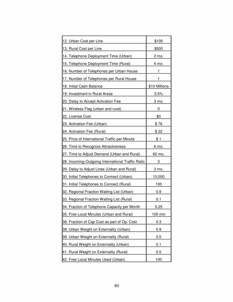
80

12. Urban Cost per Line $100

13. Rural Cost per Line $500

14. Telephone Deployment Time (Urban) 2 mo.

15. Telephone Deployment Time (Rural) 4 mo.

16. Number of Telephones per Urban House 1

17. Number of Telephones per Rural House 1

18. Initial Cash Balance $10 Millions

19. Investment in Rural Areas 3.5%

20. Delay to Accept Activation Fee 3 mo.

21. Wireless Flag (urban and rural) 0

22. License Cost $0

23. Activation Fee (Urban) $ 76

24. Activation Fee (Rural) $ 22

25. Price of International Traffic per Minute $ 1

26. Time to Recognize Attractiveness 6 mo.

27. Time to Adjust Demand (Urban and Rural) 60 mo.

28. Incoming-Outgoing International Traffic Ratio 3

29. Delay to Adjust Lines (Urban and Rural) 3 mo.

30. Initial Telephones to Connect (Urban) 10,000

31. Initial Telephones to Connect (Rural) 100

32. Regional Fraction Waiting List (Urban) 0.9

33. Regional Fraction Waiting List (Rural) 0.1

34. Fraction of Telephone Capacity per Month 0.25

35. Free Local Minutes (Urban and Rural) 100 min

36. Fraction of Cap Cost as part of Op. Cost 0.3

38. Urban Weight on Externality (Urban) 0.9

39. Urban Weight on Externality (Rural) 0.5

40. Rural Weight on Externality (Urban) 0.1

41. Rural Weight on Externality (Rural) 0.5

42. Free Local Minutes Used (Urban) 100

81

43. Free Local Minutes Used (Rural) 50

44. Expenditure on Traffic as Fr. of Income (Urb) 0.01

45. Expenditure on Traffic as Fr. of Income (Rur) 0.006

46. Fraction of Expenditure on Telecom (Urban) 0.015

47. Fraction of Expenditure on Telecom (Rural) 0.015

48. Number of People per House 4

49. Referential Price (Market Price Policy) $ 1

Table 5. Base Case values used to generate the Reference Mode

The Figure 9 shows the low levels and growth of telephones densities in

developing countries, which are less than 6 phones per 100 households in the base case

simulation. This figure indicates the telephone tendisity at the national level, which is

obtained dividing the total number of telephone lines to the total number of households

in the country. The low levels of income per capita observed in developing countries

generate low levels of financial resources to the telephone company, which are used for

telephone expansion, as shown in positive feedback loops 1 and 2 of Figure 14. This

reduces the telephone density in urban and rural areas of developing countries.

The Figure 10 shows the supply problem of telephone lines in developing

countries, where the waiting lists of subscribers are higher than the new telephone lines

available to connect. It can be seen that the gap between the waiting lists and the new

telephones installed is increasing through time. This behavior indicates the lack of

supply of new urban and rural telephone capacity because of the low levels of financial

resources of the telephone company, which are used for telecom investment, as

82

observed in positive feeback loops 1, 2, 7, and 8 in Figure 14. In addition, the rate of

new telephone subscribers in urban and rural areas depends on the monthly rental fee of

the telephone service, as seen in positive feedback loops 3 and 4 of Figure 14. It has

been observed in several developing countries that the urban monthly rental fees are

lower than the willingness to pay of the population.

The gap in telephone penetration between rural and urban areas of developing

countries is shown in Figure 11. This indicates the ratio between rural and urban

telephone densities, which is very low. It can be observed that the urban telephone

densities are higher than ten times the telephone densities in rural areas. Additionally,

the ratio between rural and urban telephone densities is decreasing, which indicates that

the regional telephone gap in developing countries is increasing. The lower income per

capita of the rural population with respect to the urban population in developing

countries, and the higher costs and obstacles experienced when deploying rural telecom

infrastructure reduce even more the rural telephone densities with respect to the urban

telephone densities, since they affect the positive feedback loops 2 and 8 in Figure 14.

83

0

45

90

135

180

0

3

6 Ph

ones

/ 10

0 H

ouse

hold

s

Months

Fig. 9. National Telephone Density of the Reference Mode

0

45

90

135

180

0

2,694,500

5,389,000

Phon

es

Months

Waiting List

New Telephone Lines

Fig. 10. Waiting List vs. New Telephone Lines of the Reference Mode

84

0

45

90

135

180

0

0.01

0.02

Months

Fig. 11. Rural-Urban Telephone Density Ratio of the Reference Mode

85

Chapter 5. The Impact of Universal Service Obligations and International Cross-

Subsidies on the Dispersion of Telephone Services in Developing Countries

As it was earlier stated, the Universal Service Obligation and International

Cross-Subsidy policies have not helped to increase the dispersion of telephone services

into rural areas. Many experiments were performed with the model described in the

previous chapter in order to see the impact of these policies on the growth of telephone

services. It was simulated several Universal Service Obligation options, with different

percentages of the total investment assigned to rural and urban regions, and several

levels of International Cross-Subsidies implemented by below cost monthly rental fees.

The base case, with no subsidy policies in place replicates the reference mode,

which is characterized by low levels and slow growth of rural and national telephone

densities. This behavior is generated by the structure of the model described in chapter

4. It represents the historical behavior described in chapter 2 over a period of nine years

or 108 months. The base case assumes a Rural Investment Fraction of 3.5 % and a

monthly rental fee of one dollar.

5.1 The Impact of Implementing Universal Service Obligations

This policy shown in Figures 12 and 13 is simulated by increasing the Rural

Investment Fraction (RIF) from 3.5, which represents the base case, to 20 and 65

percent. This increase is made, even though the ratio of willingness to pay over

operating costs is much higher in urban areas than in rural areas.

86

It is observed in Figures 12 and 13 that increasing the RIF from 3.5 % to 65 %

reduces the national telephone density from the beginning and the rural telephone

density in the very long run with respect to the base case. This happens because the

increase in this obligation reduces the revenue from telecom services and the financial

resources available for telecom investment. The decrease in financial resources not only

reduces the urban telephone density; it also diminishes the telephone density in rural

areas in the long run. The reduction of urban and rural telephone densities diminishes

the overall telephone density of the country, as observed in Figure 13.

It is important to note that a Rural Investment Fraction of twenty percent also

reduce the overall telephone density, but performs better in the long run than a Rural

Investment Fraction of 65 %. In fact, the rural telephone density is improved and the

urban and overall telephone densities are reduced again, with respect to the base case.

The RIF of 20 % reduces less the urban and overall telephone densities than a RIF of 65

%. This happens because lower values of RIF are able to maintain the overall revenues

at a higher level, which affects the rural telephone density in the long run. On the other

hand, RIF values higher than sixty five percent produce a behavior similar to the sixty

five percent case.

When the RIF is increased, the amount of money allocated for rural telecom

investment is improved with respect to the base case in the short run, as indicated by

feedback loop 2 of Figure 14. The increased investment in rural areas is achieved by

reducing the portion of investment assigned to urban telecom capacity. The additional

telecom investment assigned to rural areas turns into a lower number of new telephone

87

lines than the case when this extra amount of investment were assigned to the expansion

of the urban telephone network. This happens due to the higher costs and deployment

delays of the rural telephone lines with respect to the urban lines.

The improvement in the supply of new rural telephone lines increases the

connecting rate of telephones in rural areas and the number of rural connected

subscribers. The improved rural connecting rate tends to reduce the rural waiting list, as

observed in negative feedback loop 6 in Figure 14. The additional rural connected

subscribers improve the network externality impact in rural areas that enhances the rural

demand for telephone access and the rate of new rural customers, which tend to increase

the rural waiting list, as indicated by positive feedback loop 4.

The additional rural connected subscribers improve the rural traffic per line with

respect to the base case because of the impact of the size of the network on traffic, as

indicated by positive feedback loop 2 of Figure 14. The increase in rural connected

subscribers and rural traffic per line improves the revenue of the telephone company

from rural areas, as indicated by positive feedback loops 2 and 8 of Figure 14. However,

the extra numbers of rural connected subscribers and rural traffic per line produced by

the increase of the RIF, generate less revenue than if these extra numbers were in the

urban network. This happens because the willingness to pay for telephone services in

rural areas, which is a function of the income per capita, is lower than it is in urban

areas.

The developing countries often have weak policy implementation institutions.

This is a policy may often not be applied consistently and continuously. For this reason,

88

the increase of the Rural Investment Fraction only in the first four years is also shown in

Figures 12 and 13. It is observed in Figure 12 that the rural telephone density is

improved in the short run, but is reduced in the long term with respect to the base case.

On the other hand, as observed in Figure 13, it reduces the national telephone density

permanently. This happened because the increase of the RIF during the first four years

of the simulation reduced the financial resources with respect to the base case, which

turns into lower numbers of telephone lines and densities. The increase of the RIF

during the first four years was able to improve the rural telephone density in the short

term in spite of the reduction of financial resources, as seen in Figure 12.

5.2 The Impact of Implementing International Cross-Subsidies

As described in chapter 2, the International Cross-Subsidy is implemented by

having a below cost monthly rental fee in urban and rural areas and keeping the prices

of international telecom traffic high and at above costs levels. In this case, the

International Cross-Subsidy is implemented, even though the urban willingness to pay

for telephone access is higher than the urban monthly rental fee and the demand for

urban telephone access is relatively inelastic. The impact of this policy is shown in the

normalized values observed in Policy 2 of Table 6. This shows that the ratio of urban

operating cost to urban monthly rental fee and the ratio of urban access willingness to

pay to urban monthly rental fee are higher than one, which indicates that the urban

monthly rental fee is lower than the operating costs and the access willingness to pay in

urban areas.

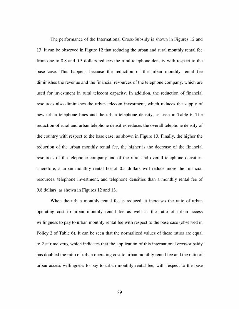
89

The performance of the International Cross-Subsidy is shown in Figures 12 and

13. It can be observed in Figure 12 that reducing the urban and rural monthly rental fee

from one to 0.8 and 0.5 dollars reduces the rural telephone density with respect to the

base case. This happens because the reduction of the urban monthly rental fee

diminishes the revenue and the financial resources of the telephone company, which are

used for investment in rural telecom capacity. In addition, the reduction of financial

resources also diminishes the urban telecom investment, which reduces the supply of

new urban telephone lines and the urban telephone density, as seen in Table 6. The

reduction of rural and urban telephone densities reduces the overall telephone density of

the country with respect to the base case, as shown in Figure 13. Finally, the higher the

reduction of the urban monthly rental fee, the higher is the decrease of the financial

resources of the telephone company and of the rural and overall telephone densities.

Therefore, a urban monthly rental fee of 0.5 dollars will reduce more the financial

resources, telephone investment, and telephone densities than a monthly rental fee of

0.8 dollars, as shown in Figures 12 and 13.

When the urban monthly rental fee is reduced, it increases the ratio of urban

operating cost to urban monthly rental fee as well as the ratio of urban access

willingness to pay to urban monthly rental fee with respect to the base case (observed in

Policy 2 of Table 6). It can be seen that the normalized values of these ratios are equal

to 2 at time zero, which indicates that the application of this international cross-subsidy

has doubled the ratio of urban operating cost to urban monthly rental fee and the ratio of

urban access willingness to pay to urban monthly rental fee, with respect to the base

90

case. This situation determines an increase in the level of international cross-

subsidization, where the telephone company becomes more dependent on above cost

international traffic and revenue. The decrease of the urban monthly rental fee

diminishes the revenue and the financial resources of the telephone company, which

reduces the gain of the positive feedback loop 7 in Figure 14. This situation diminishes

the urban telephone investment, the supply of new urban telephone lines, and the

number of urban telephone subscribers, which reduces again the revenue and financial

resources of the telephone company, as observed in positive feedback loops 1 and 7.

The diminution of financial resources also decreases the gain of positive

feedback loops 2 and 8, which diminishes the rural telephone investment, the supply of

new rural telephone lines, the connecting rate of rural telephone lines, and the number

of rural telephone subscribers, which also decrease the revenue and financial resources

of the telecom company, with respect to the base case.

91

Rural Investment Fraction = 20%

Monthly Rental Fee = $ 0.5


Base Case

Rural Investment Fraction = 20 % for TIME < 48 Months Rural Investment

Fraction = 65 %

0 45 90 135 180

0.126

0.072

0.018

Months

Phon

es /

100

Hou

seho

lds

Figure 12. Rural Telephone Density for USO and International Cross-Subisidy

Policies

Base Case

Rural Investment Fraction = 65 %


Rural Investment Fraction = 20 % for TIME < 48 Months


Rural Investment Fraction = 20 %

0

3

6

0 90 45 135 180 Months

Phon

es /

100

Hou

seho

lds

Figure 13. National Telephone Density for USO and International Cross-Subisidy

Policies

92

Figure 14. Causal Structure of Demand and Supply of the Regional Telecom

System

Urban TelecomInvestment

FinancialResources

Rural TelecomInvestment

RuralSusbcribers

UrbanSubscribers

Urban NetworkExternality Impact

Rural NetworkExternality Impact

Urban Tel ExpenditureIncrease from Size of the

Network

Rural Tel ExpenditureIncrease from Size of the

Network

+

+

Rural Traffic

Urban Traffic+

+

+

+

+

+

UrbanConnecting

Rate

RuralConnecting

Rate

Rural TelephoneCapacity

Urban TelephoneCapacity

+

+

Waiting List of UrbanSubscribers

+

Waiting List of RuralSubscribers

+

+

+

+1

+2

+3

+4

+

+

-

-

Urban Rate of NewCustomers

+ +

Rural Rate of NewCustomers

+

+

-5

-6

Rural InvestmentFrac tion

+

-

+

+

++

+8

+7

Urban MonthlyFee

+

- Urban Income

+

+

Rural MonthlyFee

-

+

Rural Income

+

+

93

5.3 Policies for Improving Telephone Penetration.

Several experiments were conducted with different pricing mechanisms and

Universal Service Obligations policies, the following results summarize the best

policies that considerably improved the regional dispersion of telephones in developing

countries. Table 6 summarizes the performance of Universal Service Obligations,

International Cross-Subsidies, Market-Clearing Pricing, and a combination of Market-

Clearing Pricing with Universal Service Obligations.

5.3.1 Market-Clearing Pricing

This policy is implemented by defining the urban monthly rental fee as a

function of the supply of additional urban telephone capacity, which depends on the

financial resources, and demand for urban telephone capacity, which is a function of the

urban waiting list of telephone subscribers. Figure 15 shows the behavior of the urban

monthly rental fee when the market pricing mechanism is applied. The base case

represents the behavior of a regulated and fixed monthly fee of one dollar. Figure 16

shows the feedback structure driving changes in monthly rental fee.

Whenever the market pricing mechanism is applied to urban areas, the urban

monthly rental fee is increased when the ratio between the supplied urban telephone

capacity and the demanded urban telephone capacity is lower than one. When supply of

additional urban lines equals the demand for them, the monthly rental fee is assumed to

be equal to a reference price of one dollar. When the financial resources are large

enough, such that the supplied urban telephone capacity could be higher than the

94

demanded urban telephone capacity, the lower the urban monthly rental fee is, as

indicated in the structure shown in Figure 16.

It is observed in Figure 16 that the increase of the urban monthly rental fee will

tend to reduce the growth of urban potential telephone subscribers and improve the

financial resources of the telephone company. The diminution of urban potential

telephone subscribers decreases the gain of positive feedback loop 11, which reduces

the urban waiting list and the demanded urban telephone capacity. On the other hand,

the improvement in the financial resources increases the supply of urban telephone

capacity. The augment of the supply of urban telephone capacity and the reduction of

the demanded urban telephone capacity decrease the urban monthly rental fee in the

long run, as observed in Figure 15. This improves the number of urban potential

subscribers, the urban waiting list, and the demanded telephone capacity in urban areas

also in the long run, as indicated by positive feedback loop 11 in Figure 16. This

situation considerably increased the urban telephone density, the rural telephone

density, the national telephone density, and the financial resources of the telephone

company, as observed in the normalized values of Policy 3 in Table 6.

It is observed in Policy 3 ofTable 6 that the increase of the urban monthly rental

fee through market pricing considerably improves the financial resources and the

telephone densities of the telephone company with respect to the base case. For instance

at year 15, the national telephone density was increased from its normal value of 12.32

(Base Case) to 44.31 (Policy 3), and the financial resources were increased from 3.86

(Base Case) to 63.40 (Policy 3). The increase of the monthly rental fee in urban areas

95

has little effect on urban access demand, since this is relatively inelastic and the

willingness to pay for urban telephone access is higher than the urban monthly rental

access fee, as observed in Table 6.

The base case shows that the ratio of urban access willingness to pay to urban

monthly rental fee is higher than 1. When the market pricing policy is applied to urban

areas, it increases the urban monthly rental fee, which reduces this ratio in the short

term and enlarges the financial resources and telephone densities of the telecom

company. The growth of telephone densities enhances the network externality impact,

which improves the willingness to pay for telephone access in urban areas. The

improvement of the urban access willingness to pay and the reduction of the urban

monthly rental fee in the long run, improve the ratio of urban access willingness to pay

to urban monthly rental fee also in the long run, as observed in the normalized values of

Policy 3 in Table 6.

5.3.2 Market-Clearing Pricing with Universal Service Obligation.

This policy considers the market-clearing pricing policy described in the

previous section, combined with an implementation of USO, which increases the RIF

only after the urban telephone density reaches thirty percent. This means that thirty over

100 households have a telephone line. This level of connectivity occurs when the supply

of telephone capacity in urban areas equals the demanded urban telephone capacity

using a market-clearing pricing mechanism.

96

The addition of this particular implementation of USO to the market-clearing

policy improves considerably the rural telephone density and the rural-urban telephone

density gap in the long term with respect to the implementation of market-clearing

pricing alone, without reducing the number of urban telephone lines and urban

telephone density, as shown in the normalized values of Policies 3 and 4 in Table 6. The

rural telephone density was improved from its normalized value of 19.72 (Policy 3) to

57.56 (Policy 4) in year 15, and the rural-urban telephone density gap was improved

from 0.53 (Policy 3) to 1.53 (Policy 4) also in year 15. In fact, it slightly improves the

national telephone density in the long run.

After the urban supply of telephone capacity equals the urban telephone demand

when the market-clearing pricing is applied to urban areas, the financial resources

considerably improve because the number of urban telephone lines has been increased

by the action of positive feedback loops 1 and 7 in Figure 14, and the urban waiting list

has been reduced by the action of negative feedback loop 10 in Figure 16.

The improvement of the financial resources to a level where the supply of urban

telephone capacity equals the demanded urban telephone capacity reduces the strength

of negative feedback loops 9 and 10 in Figure 16. The excess of financial resources can

now be used to satisfy the rural waiting list by increasing the RIF, which improves the

rural telecom investment and rural telephone lines and density. This situation raises the

gain of positive feedback loops 2 and 8 in Figure 14, which increases the rural

connecting rate and the gain of negative feedback loop 6, reducing the rural waiting list

at the same time. However, the improvement of rural investment in the long term

97

diminishes the financial resources with respect to application of market-clearing pricing

alone. This can be observed in the normalized values of financial resources

corresponding to Policies 3 and 4 in Table 6. The financial resources are reduced from

63.40 (Policy 3) when the market price is implemented alone to 41.27 (Policy 4) when

market pricing is combined with the increasing of the rural investment fraction when

the telephone density reaches thirty percent.

Base Case

Market-Clearing Pricing

Market-Clearing Pricing with USO

3

1.5

0

1

0 45 90 135 180 Months

Dol

lars

Figure 15. Market and Fixed Monthly Rental Prices

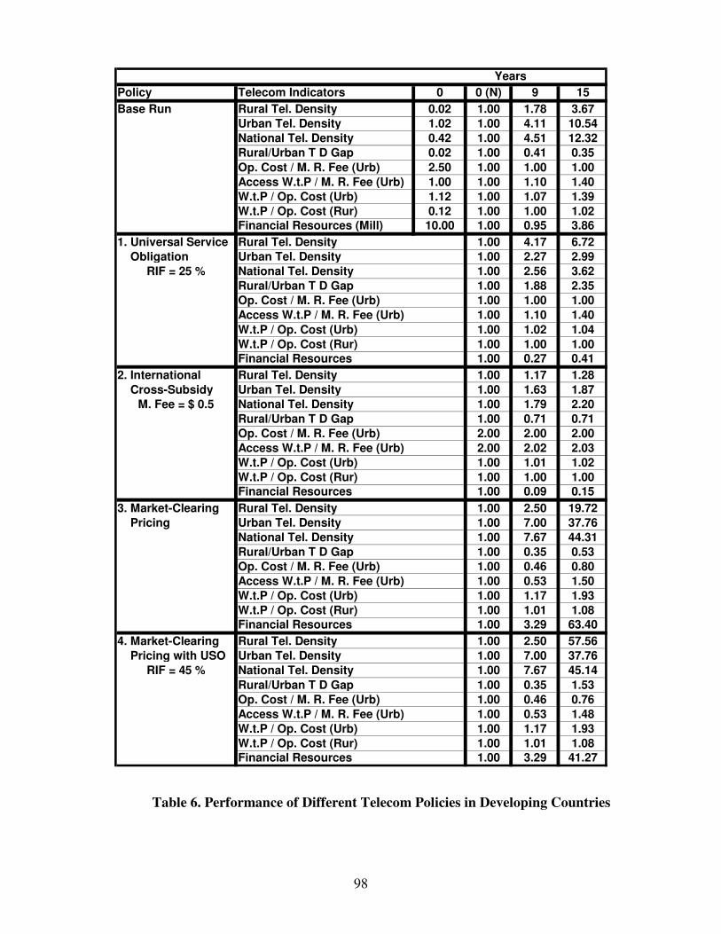
98

Table 6. Performance of Different Telecom Policies in Developing Countries

Policy Telecom Indicators 0 0 (N) 9 15Base Run Rural Tel. Density 0.02 1.00 1.78 3.67

Urban Tel. Density 1.02 1.00 4.11 10.54National Tel. Density 0.42 1.00 4.51 12.32Rural/Urban T D Gap 0.02 1.00 0.41 0.35Op. Cost / M. R. Fee (Urb) 2.50 1.00 1.00 1.00Access W.t.P / M. R. Fee (Urb) 1.00 1.00 1.10 1.40W.t.P / Op. Cost (Urb) 1.12 1.00 1.07 1.39W.t.P / Op. Cost (Rur) 0.12 1.00 1.00 1.02Financial Resources (Mill) 10.00 1.00 0.95 3.86

1. Universal Service Rural Tel. Density 1.00 4.17 6.72 Obligation Urban Tel. Density 1.00 2.27 2.99

RIF = 25 % National Tel. Density 1.00 2.56 3.62Rural/Urban T D Gap 1.00 1.88 2.35Op. Cost / M. R. Fee (Urb) 1.00 1.00 1.00Access W.t.P / M. R. Fee (Urb) 1.00 1.10 1.40W.t.P / Op. Cost (Urb) 1.00 1.02 1.04W.t.P / Op. Cost (Rur) 1.00 1.00 1.00Financial Resources 1.00 0.27 0.41

2. International Rural Tel. Density 1.00 1.17 1.28 Cross-Subsidy Urban Tel. Density 1.00 1.63 1.87

M. Fee = $ 0.5 National Tel. Density 1.00 1.79 2.20Rural/Urban T D Gap 1.00 0.71 0.71Op. Cost / M. R. Fee (Urb) 2.00 2.00 2.00Access W.t.P / M. R. Fee (Urb) 2.00 2.02 2.03W.t.P / Op. Cost (Urb) 1.00 1.01 1.02W.t.P / Op. Cost (Rur) 1.00 1.00 1.00Financial Resources 1.00 0.09 0.15

3. Market-Clearing Rural Tel. Density 1.00 2.50 19.72 Pricing Urban Tel. Density 1.00 7.00 37.76

National Tel. Density 1.00 7.67 44.31Rural/Urban T D Gap 1.00 0.35 0.53Op. Cost / M. R. Fee (Urb) 1.00 0.46 0.80Access W.t.P / M. R. Fee (Urb) 1.00 0.53 1.50W.t.P / Op. Cost (Urb) 1.00 1.17 1.93W.t.P / Op. Cost (Rur) 1.00 1.01 1.08Financial Resources 1.00 3.29 63.40

4. Market-Clearing Rural Tel. Density 1.00 2.50 57.56 Pricing with USO Urban Tel. Density 1.00 7.00 37.76

RIF = 45 % National Tel. Density 1.00 7.67 45.14Rural/Urban T D Gap 1.00 0.35 1.53Op. Cost / M. R. Fee (Urb) 1.00 0.46 0.76Access W.t.P / M. R. Fee (Urb) 1.00 0.53 1.48W.t.P / Op. Cost (Urb) 1.00 1.17 1.93W.t.P / Op. Cost (Rur) 1.00 1.01 1.08Financial Resources 1.00 3.29 41.27

Years

99

Figure 16. Feedback Loops affecting Urban Telephone Capacity

5.3.3 Formulation of Market-Clearing Pricing

The market-clearing pricing mechanism (MCP) adjusts this price towards an

indicated monthly rental fee (IMRF), which is a function of the current monthly rental

fee (MRF) and a non-linear function of the ratio between the supplied telephone

capacity (STC) and the demanded telephone capacity (TCD). The time to adjust market

price (TAP) depends on this non-linear function and a referential time to adjust market

price (RTAP):

(d / dt)MCP u = (IMRF – MCP u) / TAP i (43)

IMRF = MRF * f 4 (STC i / TCD i)

UrbanConnecting Rate

FinancialResources

Urban WaitingList

Urban TelephoneCapacity

Urban ConnectedSubscribers

Urban PotentialSubscribers

-+

+ +

-

+

-9

+11

-10

Urban SuppliedTelephone Capacity

+

+

Urban DemandedTelephone Capacity

+

+

Market Price

- +

-

+

+

100

TAP i = RTAP * (1 + f 4 (STC i / TCD i)), Where f ’5 is < 0

5.3.4 Sensitivity of Policies for Improving Rural Telecommunications

An important instrument in the policy framework outlined in the preceding

section is the application of market-clearing pricing to urban areas, which improves the

revenue and the financial resources of the telecom company reducing the urban unmet

demand at the same time. In addition, the market-clearing pricing combined with

animplementation of USO was able to improve the rural telephone density without

diminishing the urban telephone density.

New experiments were conductedto test the sensitivity of market-clearing

pricing combined with USO, to changes in the urban income per capita, cost of

providing service, deployment time of telephone lines, and the network externality

impact. The network externality impact is a non-linear function of the telephone

density, which improves the attractiveness and demand of the telephone service and the

expenditure on telephone traffic, as the telephone density increases. The urban income

per capita, deployment time and cost of telephone lines were increased, and the network

externality impact was reduced (the slopes of the curves that define this impact in urban

and rural areas, which are shown in the appendix, were reduced).

The urban income per capita was increased from 550 dollars to 1,500 dollars, the

deployment time was increased from two to four months in urban areas and from four to

six months in rural areas, the cost of a telephone line was increased from 100 to 150

101

dollars in urban areas and from 500 to 700 dollars in rural areas. The simulation results

of this sensitivity analysis are summarized in the normalized values of Table 7.

It is observed in Table 7 that the application of market-clearing pricing to urban

areas, shown in Policy 1, stillimproves both the urban and rural telephone densities with

respect to the base case. It can be seen in year 15, that the rural telephone density is

increased from its normalized value of 18.22 (Base Case) to 40.28 (Policy 1), and the

urban telephone density is increased from its normalized value of 36.88 (Base Case) to

40.39 (Policy 1), when market pricing is applied. The market-clearing pricing

mechanism initially increases the urban monthly rental fee and later reduces it. This

improves the financial resources and the number of telephone lines, and reduces the

unmet demand.

The implementation of market-clearing pricing combined with the

implementation of USO when the urban telephone density reaches thirty five percent is

shown in Policy 2. This appears to considerably increase the rural telephone density and

the rural-urban telephone density gap in the long term compared with the application of

market-clearing pricing alone. It is observed in the normalized values of Policies 1 and

2 in year 15 that the rural telephone density is increased from 40.28 (Policy 1) to 161.33

(Policy 2), and the rural-urban telephone density gap is improved from 1 (Policy 1) to

4.12 (Policy 2). When market pricing is combined with USO, the financial resources are

reduced with respect to the application of market pricing alone. It can be seen in Table 7

that the normalized values of financial resources are reduced from 244.20 (Policy 1) to

130.20 (Policy 2).

102

Table 7. Performance of Market-Clearing Pricing Polices for Higher Income per

Capita, Implementation Costs and Deployment Times, and Lower Network

Externality Impact.

5.3.5 Conclusions

Governments and international organizations often attempt to achieve the

universal service and increase the rural telecom infrastructure in developing countries

by implementing Universal Service Obligations and International Cross-Subsidies.

These organizations, however, do not have a clear understanding of the implications and

Policy Telecom Indicators 0 0 (N) 9 15Base Run Rural Tel. Density 0.02 1.00 2.83 18.22

Urban Tel. Density 1.02 1.00 7.39 36.88National Tel. Density 0.42 1.00 8.10 43.24Rural/Urban T D Gap 0.02 1.00 0.35 0.47Op. Cost / M. R. Fee (Urb) 3.75 1.00 1.00 1.00Access W.t.P / M. R. Fee (Urb) 7.63 1.00 1.18 1.78W.t.P / Op. Cost (Urb) 2.03 1.00 1.18 1.78W.t.P / Op. Cost (Rur) 0.11 1.00 1.02 1.06Financial Resources (Mill) 10.00 1.00 6.19 141.60

1. Market-Clearing Rural Tel. Density 1.00 3.28 40.28 Pricing Urban Tel. Density 1.00 8.98 40.39

National Tel. Density 1.00 9.83 47.81Rural/Urban T D Gap 1.00 0.35 1.00Op. Cost / M. R. Fee (Urb) 1.00 0.47 0.80Access W.t.P / M. R. Fee (Urb) 1.00 0.58 1.55W.t.P / Op. Cost (Urb) 1.00 1.26 1.80W.t.P / Op. Cost (Rur) 1.00 1.02 1.07Financial Resources (Mill) 1.00 9.26 244.20

2. Market-Clearing Rural Tel. Density 1.00 3.28 161.33 Pricing with USO Urban Tel. Density 1.00 8.98 40.39

RIF = 45 % National Tel. Density 1.00 9.83 50.52Rural/Urban T D Gap 1.00 0.35 4.12Op. Cost / M. R. Fee (Urb) 1.00 0.47 0.87Access W.t.P / M. R. Fee (Urb) 1.00 0.58 1.55W.t.P / Op. Cost (Urb) 1.00 1.26 1.80W.t.P / Op. Cost (Rur) 1.00 1.02 1.07Financial Resources (Mill) 1.00 9.26 130.20

Years

103

impacts of such policies. The Universal Service Obligation policy increases the

percentage of investment in rural areas, while reducing the percentage in urban areas.

The International Cross-Subsidy policy maintains the international service prices high

while keeping the urban monthly rental fee below the urban operating cost and urban

willingness to pay for telephone access values. We found that these policies are

counterproductive because of they limit growth in service due to financial constraints

they create.

The simulations showed that market-clearing pricing applied to urban areas was

able to considerably improve the number of rural and urban telephone lines and the

financial resources of the telecom company. However, if the Universal Service

Obligation policy is implemented simultaneously after the urban telephone density

reaches thirty percent, while the supply of urban telephone capacity equals the

demanded capacity, a considerable increase of rural telephone density is obtained.

The findings of this research are useful for telecom operators and regulators,

since they can identify the pervasive impact of cross-subsidies on the dispersion of

telephone services. However, the actual implementation of these policies and strategies

in real life requires the model to be constantly updated to capture changes in telecom

policies and technologies.

More research under new and different scenarios is needed in order to identify

new strategies and policies that could increase telephone dispersion in developing

countries. The investigation of new pricing mechanisms and service combinations that

could improve telephone penetration in developing countries will be of value. The

104

impact of competition and quality of service are other important issues that can be

addressed by extending the model presented in this dissertation.

105

Chapter 6. A Value Added Service Strategy for the Improvement of Telephone

Density in Rural Areas of Developing Countries.

6. 1 Abstract

Telephone densities in developing countries are typically extremely low. This is

often a consequence of poor planning and inadequate pricing policies. The regional

telecom model is extended to deal with the complexity of the telecommunication system

in a developing country, giving special attention to the discrepancies between urban and

rural areas. This model is used to test several combinations of service offerings and

pricing policies that exploit positive feedback loops of the telecom system. Simulations

suggest that the dispersion of telephone services in rural areas may significantly

improve when a prepaid pricing scheme is applied simultaneously to the telephone,

virtual telephony, and the payphone services. Other schemes are also tested but fail to

bring significant improvements to the underdeveloped telecommunication system.

6.2 Introduction

The current policies and technologies for increasing telecommunications

deployment in rural areas are considered to be insufficient or unsuccessful, and the

plans for expansion of local telephone networks are considered to be imprecise

considering the scope of the investment (Malecki, 2003; Melody, 1999; Strover, 2003;

Calhoun, 1992). However, the value added services (VAS) are considered to have the

potential to increase the telephone access in developing countries, but it is still not clear

106

if they will be able to improve the telephone density in unprofitable rural areas and

reduce the rural-urban telephone density gap after their implementation.

In some cases, the low level of telephone penetration in developing countries has

been attributed to an outdated telecommunications system that prevents development of

value added services, which are supposedly able to generate more revenue required for

telecom investment (Fretes-Cibils et. al., 2003). In some cases, the resources invested in

value added services, or intelligent network platform, have been considered worthwhile

after the revenue of the telecom company is increased, and better service to the

subscribers is provided (Hamersma, 1996). In spite of this, there are few studies that

have been developed in order to assess the impact that these innovative solutions have

on increasing the connectivity of nations (Barendse, 2004).

The impact of pricing structures on the adoption of mobile telephones has not

received much attention in the past (Hodge, 2005). The prepaid pricing alternative

provides an opportunity for individuals to manage their telephone expenses, since the

number of calls that can be made is restricted. This and the relatively simple

subscription process generate a broad customer acceptance for prepaid phone services

(Hamilton, 2003). In this dissertation, Systems Dynamics is used to investigate the

prepaid pricing mechanism of telephone services, which could be used to design a value

added service strategy that considerably improves the number of rural telephone lines

based on the synergic impact ofthese services on network externality of the regional

telephone system.

107

It was found that the implementation of prepaid phone, virtual telephony, and

payphone services together significantly improved the financial resources of the

telephone company and accelerated the rural dispersion of telephone services in

developing countries. However, the success of this strategy will depend on the

friendliness of the user interface and the availability of these services in the region.

Finally, it is important to note that the implementation of these services in isolation only

achieved a moderate improvement.

6.3 Value Added Services in Telecommunications

The provision of value added services, such as voice mail, virtual telephony,

prepaid phone, and payphone services, among others, represent an opportunity to

improve the productivity or revenue from the local loops, and provide extra value or

better service to the subscribers. The implementation of value added service platforms,

which are called intelligent networks (IN), involves improving this network and

introducing new services on this platform (Thorner, 1994).

The low level of telephone penetration in a country has sometimes been

attributed to the fact that the telecommunications network is outdated. This prevents the

deployment of value added services (Fretes-Cibils et. al., 2003). There is certain

evidence that the introduction of prepaid phone services in mobile telephony has been

able to expand the number of telephone lines in developing countries. However, the

actual impact of this innovative pricing mechanism, which uses a VAS platform, is still

unclear (Hodge, 2005). The Table 8 shows the growth of prepaid and postpaid cellular

108

phones in selected developing countries (World Telecommunication Indicators

Database, 2004). It can be observed the exponential growth of prepaid telephones,

which is much higher than the growth of postpaid phones. In addition, it can also be

observed in this table the increasing gap between the number of prepaid and postpaid

telephones through years.

There is a management trend in developing countries to overlook or delay the

provision of valued added services, since the focus has been to address the large number

of waiting lists or outstanding demand in the system (Saunders et. al., 1994). For

instance, the investment in payphone services, which use the intelligent network

platform, has been very low. The Table 9 shows the low level of penetration of

payphone devices in selected developing countries, although there has been some

growth. The penetration of payphones in developing countries is much lower than the

penetration of payphones in developed countries, which is generally higher than two

payphones per 1000 people (World Telecommunication Indicators Database, 2004).

The investment in value added services reduces the investment in telecom

expansion but there is a potential to increase the financial resources of the telephone

company in the long run. In addition, there is a belief in the telecom industry that

investment in more advanced VAS from revenue generated in basic services, such as

telephony, could divert the focus from the expansion of basic telecom infrastructure and

universal service (Siochru, 1996). For this reason, the investment cost of the VAS

platform needs to be trade-off against the potential increase of revenue and provision of

better services to the subscribers (Hamersma, 1996).

109

In spite of the potential benefits that value added services could provide to the

expansion of telephone services in developing countries, there are few studies

developed in order to assess the impact that these innovative solutions have on

increasing telecom penetration in these nations (Barendse, 2004). This research will

study the impact of three different services: virtual telephony, payphone, and prepaid

phone services.

The VAS studied in this dissertation target different markets and need several

VAS infrastructures. The prepaid payphone service is offered to the population who is

not interested in subscribing to the telephone service. This service requires the

deployment of calling card numbers and public payphones. In addition, the virtual

telephony service is offered to subscribers in the waiting list. This service is a

combination of voice mail and payphone services. Therefore, it requires the deployment

of mailboxes, calling card numbers, and public payphones. Finally, the prepaid phone

service is offered to the population who does not have a telephone and is able to use

this. This service requires the same infrastructure as the conventional postpaid

telephone service and the deployment of calling card numbers, which is implemented in

the intelligent network platform.

110

Table 8. The Dispersion of Prepaid Cellular Phones in Selected Developing

Market Economies.

Source: World Telecommunication Indicators Database (2004).

Table 9. The Dispersion of Payphones in Selected Developing Market

Economies.

Source: World Telecommunications Indicators Database (2004).

6.4 Impact of Value Added Services on Telephone Expansion

In this section, several experiments were conducted with different value added

service implementations, which did not strategically consider the interactions and

feedback loops of the regional telecommunications system. The base case, which

indicates a cellular service without VAS implementation, is shown at the top of Table

10.

Prepaid-Postpaid Prepaid-PostpaidCountries Prepaid Postpaid Ratio (1998) Prepaid Postpaid Ratio (2002) Prepaid Postpaid

Togo 6000 1500 4 168000 2000 84 2700 33Bolivia 112247 127025 0.9 674710*** 105207*** 6.4*** 501 -17Ecuador 18450* 108055* 0.2* 1272333 288528 4.4 6796 167Honduras 11875 23021 0.5 259156 67352 4 2082 192Thailand 391000** 2665000** 0.15** 12735000 3382000 4 3157 26* year 1997, ** year 2000, *** year 2001

2002-1998 Growth (%)20021998

1998-1993 2002-1998Countries 1993 Payph/1000 pe 1998 Payph/1000 pe 2002 Payph/ 1000 pe Payph Growth Payph GrowthZambia 526 0.06 554 0.05 878 0.08 0.05 0.58Togo 68 0.01 132 0.03 12257 2.5 0.94 91.85India 172000 0.1 527000 0.5 2006000 1.9 2.06 2.8

Bangladesh 1982 0.01 2023 0.01 2208 0.01 0.02 0.09Pakistan 6000 0.04 28000 0.2 99000 0.6 3.66 2.53Ecuador 3024 0.2 3846 0.3 5003 0.3 0.27 0.3

Honduras 861 0.1 2582 0.4 2583 0.3 2 0Botswana 528 0.3 2449 1.5 2242 1.3 3.63 -0.08

Payphones

111

6.4.1 Payphone Service

The prepaid payphone service uses payphones and calling card numbers as basic

infrastructure. This service is intended for each person capable of using a payphone,

who is not interested on being a subscriber of the current telephone service. The

potential subscribers are attracted to the payphone service after considering its price,

user-friendly interface, availability, and the number of subscribers reachable in the

network, which is represented in the model by the network externality impact. The

higher the network externality impact, the higher the number of people reachable in the

network. This service is implemented in the model by setting the VAS Offered variable

for Payphone services in both urban and rural areas to 1, and by increasing the VAS

investment referential variable to 0.04. The VAS investment referential variable

considers payphones as the only significant value added service infrastructure in terms

of costs and deployment delays.

The total price paid by the payphone subscribers for the total number of calling

cards used is relative to the willingness to pay for fixed telephone services, which

depends on the network externality impact. The network externality is a function of the

telephone density in the region (Saunders et. al., 1994). It is observed in Figure 17 that

the number of telephone subscribers in the network affects the network externality

impact of the system. The higher the telephone density and the network externality

impact, the higher the willingness to pay for fixed telephone services and the number of

calling cards consumed by the payphone subscribers. In addition, the payphone

112

subscribers consume an amount of prepaid calling cards based on the willingness to pay

for fixed telephone services. The money spent in prepaid calling cards is called the

payphone price in the model.

The performance of payphone services on the regional telecommunications

system is observed in VAS 1 of Table 10. The national and regional telephone densities

show a moderate improvement after the payphone service implementation, since the

financial resources used for telephone expansion have been increased. For instance, in

year 15, the financial resources were increased from its normalized value of 1.320 (Base

Case) to 3.529 (VAS 1). On the other hand, the rural-urban telephone density gap is not

improved in spite of the rural telephone density growth. This indicates that the

improvement of financial resources is not strong enough to reduce also the rural-urban

telecom gap.

The higher the number of telephones in the region the higher the network

externality impact, which improves the payphone demand and the willingness to pay for

fixed telephone services, as observed in positive feedback loops 17 and 18 of Figure 17.

The enhancement on willingness to pay for fixed telephone services increases the

number of prepaid payphone cards used in the system, which expands the payphone

price. This situation enlarges the financial resources of the telephone company, as

observed in positive feedback loop 18.

The improvement on payphone demand increases the number of payphone users,

which also expands the financial resources of the telephone company because the

revenue from payphone services is augmented, as observed in positive feedback loops

113

13 and 17 of Figure 17. As described before, the expansion of financial resources

improves the number of telephone lines. The investment in payphone infrastructure is

subtracted from the investment in telephone expansion, as shown by negative feedback

loop 16 of Figure 17.

Figure 17. Payphone Service Impact on Telephone Expansion

6.4.2 Virtual Telephony Service

The virtual telephony service is a form of fixed telephone service, which

is a combination of voice mail and prepaid payphone services. This implies that virtual

telephony requires mailboxes, payphones, and calling cards, as basic infrastructure. This

service targets telephone subscribers in the waiting list, who have decided to subscribe

FinancialResources

Investment inTe lephone Lines

New Lines

+

+

Telephone Lines+

+

Investment inPayphones

+

- -

PayphoneInfrastructure

PayphoneAvailability

+

+

PayphoneDemand

+

PayphoneUsers+

++12

-15-14

+13

--16


+17

PayphonePrice

+

Willingness to PayFixed Telephony

+

++18+

Easy to UseFactor

+

114

to the service and to pay for the telephone device and activation fee, but the telephone

company has not connected them yet. This service is implemented in the model by

setting the VAS Offered variable for Virtual Telephony services in both urban and rural

areas to 1, and by increasing the VAS investment referential variable to 0.04. The VAS

investment referential variable considers payphones as the only significant value added

service infrastructure in terms of costs and deployment delays.

The subscribers of virtual telephony were attracted to this service after

considering its price, and other features such as user-friendly interface and availability.

The price paid for the virtual telephony service is proportional to the willingness to pay

for the fixed telephone service, which depends on the network externality impact. The

virtual telephony users consume a number of calling cards relative to this willingness to

pay. It is observed in Figure 18 that the number of telephone subscribers in the network

affects the network externality impact of the system. The virtual telephony subscribers

consume an amount of prepaid calling cards based on the willingness to pay for fixed

telephone services. This determines the amount of money spent on these cards, which is

called the virtual telephony price in the model.

The performance of virtual telephony on the regional telecommunications

system is observed in VAS 2 of Table 10. It is observed that the virtual telephony

service is able to slightly improve in the long term the national and regional telephone

densities, and the rural-urban telephone density gap is not improved. For instance, in

year 9, the rural telephone density is reduced from its normalized value of 14.545 (Base

Case) to 14.091 (VAS 2), and the urban telephone density is slightly improved from its

115

normalized value of 9.501 (Base Case) to 9.552 (Virtual Telephony). However in year

15, the rural telephone density is somewhat improved from 33.455 (Base Case) to

34.182 (VAS 2). The telephone density improvement is relative to the expansion of

financial resources, which depends on the number of virtual telephony users and the

price charged for the virtual telephony service, as observed in Figure 18.

The financial resources are not improved with respect to the base case, in spite

of the minimum improvement on telephone densities. The increase of telephone

densities is too low to improve the telephone revenue and the financial resources during

the first fifteen years of the simulation. On the other hand, the increase on telephone

densities and virtual telephony users enlarges the telephone expenses, in the form of

telecom investment and operating costs. The Table 10 shows that in year 15, after the

application of virtual telephony, the financial resources are still lower than the base

case.

The simulations proved that the impact of virtual telephony on the system is low,

which is described as follows. The growth in the number of virtual telephony and

telephone subscribers improve the impact of network externality on the system, as

observed in positive feedback loops 23 and 25 of Figure 18. This situation enhances

telephone demand and the number of telephone subscribers in the network, which is

shown in positive feedback loop 22. The improvement on telephone demand enlarge the

number of potential telephone subscribers and the quantity of telephone subscribers in

the waiting list, which also augment the number of virtual telephony users, as observed

in positive feedback loop 24 in Figure 18. The higher network externality impact also

116

increases the willingness to pay for fixed telephone services, which improves the

number of calling cards used by the virtual telephony subscribers. This situation is

represented by the virtual telephony price observed in positive feedback loops 23 and

25 in Figure 18.

Figure 18. Virtual Telephony Service Impact on Telephone Expansion

6.4.3 Virtual Telephony and Payphone Services

The combination of virtual telephony and payphone services is simulated in the

model and is shown in VAS 3 of Table 10. It can be seen that the combination of these

two services performs better than the implementation of each of these in isolation,

which are shown in VAS 1 and VAS 2. It is observed that the national and regional

FinancialResources

Investment inTe lephone Lines

New Lines

+

+

Telephone Lines++

Investment inVirtual Telephony

+

--Virtual Telephony

Infrastructure

Virtual TelephonyAvailability

+

+

Virtual TelephonyDemand

+

VirtualTe lephony Users

+

+

+12-15-20

+19

V. TelephonyPrice

+

--21

Te lephoneDemand


+

+

+

Willingness to PayFixed Telephony

+

++22+23+

+24+

+25Easy to Use

Factor

+

+

117

telephone densities, and financial resources are improved with respect to the

implementation of these services in isolation. However, the rural-urban telephone

density gap is not reduced in spite of the rural telephone density growth.

The functioning of these two services was described in previous sections.

However, it is important to emphasize that both services share a specific VAS

infrastructure deployed in the region, the payphones. The sharing of this infrastructure

makes the use of payphones more productive, since the investment in costly payphones

is being recovered from revenue generated from both virtual telephony and payphone

services, which is a result of the conjoint action of positive feedback loops 13, 17, 18,

19, 23, and 25 in Figures 17 and 18. This situation improves the financial resources of

the telephone company, which is used for VAS and telephone expansion.

When these two services are combined, the number of virtual telephony

subscribers enhances the network externality impact, as shown in positive feedback

loop 24 of Figure 18. This improves the number of payphone users and the number of

calling cards consumed by payphone subscribers, as observed in positive feedback

loops 17 and 18 in Figure 17. This situation expands the financial resources of the

telephone company and the number of telephone lines. The higher number of telephone

lines strengthens even more the network externality impact, as observed in positive

feedback loops 17, 18, and 25 in Figures 17 and 18.

118

6.4.4 Prepaid Phone Service

This service consists on the use of a VAS infrastructure implemented in the

intelligent network of the telephone company, the prepaid calling card. The prepaid

calling card is used as a mechanism of pricing, which replaces the conventional

postpaid scheme. This service uses calling cards as basic infrastructure, where each

subscriber will consume an amount of cards proportional to his/her willingness to pay.

This service is implemented in the model by setting the VAS Offered variable for

Prepaid Phone services in both urban and rural areas to 1, and by resetting the VAS

investment referential variable to 0.

The prepaid cellular telephone service is implemented in parallel to the

conventional postpaid cellular telephone service. The prepaid phone service allows

subscribers not interested in the postpaid service, because of the commitment to pay the

monthly rental fee and complex paper work requirement, to become interested in the

telephone service according to their willingness to pay. It is important to note that the

subscription process of this prepaid service does not involve major paper work and is

usually delivered in a simple service pack.

The performance of the prepaid telephone service is observed in VAS 4 of Table

10. It can be seen that the implementation of a prepaid telephone service improves

considerably the regional and national telephone densities, and the financial resources,

in the long term with respect to other VAS implementations. However, the rural-urban

telephone density gap disimprove since the urban telephone density has increased in a

larger proportion than the rural density. For instance in year 15, the normalized

119

financial resources increased to 6.434 (VAS 4), which is much higher than the base case

value of 1.32, and higher than the value of 4.178, obtained from the combined

implementation of virtual telephony and payphones. The rural telephone density

increased from the normalized value of 33.455 (Base Case) to 107.364 (VAS 4), and the

rural-urban telephone density ratio reduced from 1.481 (Base Case) to 1.111 (VAS 4).

The relatively simple subscription process and the price based on the willingness

to pay of the prepaid telephone service reduce the adoption delay with respect to the

postpaid telephone service. This situation expedites the adoption of telephone lines for a

prepaid telephone service, as observed in positive feedback loop 27 in Figure 19. In

addition, the higher the willingness to pay for telephone services, the higher the number

of prepaid calling cards demanded by the prepaid subscribers, as observed in positive

feedback loops 26 and 27 of Figure 19. The higher the prepaid telephone service price,

or the number of calling cards used, the higher the revenue and financial resources of

the telephone company, which are used for telephone expansion.

The telephone expansion achieved by the improvement of the financial resources

enhances the network externality impact of the system, as seen in positive feedback

loops 26 and 27 of Figure 19. The higher network externality impact increases the

willingness to pay for telephone services and the number of calling cards consumed by

the prepaid subscribers. On the other hand, the improvement of the network externality

impact increases the postpaid and prepaid telephone demand, which expands the

number of postpaid and prepaid telephone lines respectively, as observed in positive

feedback loops 28 and 29

120

.

Figure 19. Prepaid Phone Service Impact on Telephone Expansion

FinancialResources

Investment inTe lephone Lines+

Telephone Lines

+

Willingness to Payfor Te lephones

Prepaid PhonePrice

+

++26


+

+

New PostpaidPhone Lines

New PrepaidPhone Lines+

+

+

+

Postpaid PhoneDemand

+

+

Prepaid PhoneAdoption Delay

Postpaid PhoneAdoption Delay

-

-

Prepaid PhoneDemand

+

+

+27

+28

-

-15

+29 Easy to UseFactor

+

121

Table 10. Impact of Different Value Added Services on Telephone Expansion

Base Run Rural Tel. Density 1.000 11.000 14.545 33.455Urban Tel. Density 1.000 6.292 9.501 25.592National Tel. Density 1.000 6.599 10.212 28.525Rural/Urban T D Ratio 1.000 1.852 1.852 1.481Financial Resources 1.000 0.099 0.223 1.320

1. Payphones Rural Tel. Density 1.000 10.636 15.727 53.364Urban Tel. Density 1.000 6.232 10.836 43.711National Tel. Density 1.000 6.535 11.631 48.664Rural/Urban T D Ratio 1.000 1.852 1.852 1.481Financial Resources 1.000 0.125 0.330 3.259Payphones/ 1000 people 0 0.067 0.096 0.325

2. Virtual Rural Tel. Density 1.000 10.636 14.091 34.182Telephony Urban Tel. Density 1.000 6.232 9.552 27.518

National Tel. Density 1.000 6.535 10.258 30.641Rural/Urban T D Ratio 1.000 1.852 1.852 1.481Financial Resources 1 0.092 0.219 1.437Payphones/ 1000 people 0 0 0 0

3. Virtual Rural Tel. Density 1.000 10.909 16.091 63.455Telephony and Urban Tel. Density 1.000 6.516 11.592 53.569Payphones National Tel. Density 1.000 6.829 12.433 59.631

Rural/Urban T D Ratio 1.000 1.852 1.481 1.481Financial Resources 1 0.128 0.367 4.178Payphones/ 1000 people 0.000 0.067 0.098 0.382

4. Prepaid Rural Tel. Density 1.000 7.636 15.455 107.364Phones Urban Tel. Density 1.000 7.722 15.150 97.082

National Tel. Density 1.000 7.995 16.147 107.880Rural/Urban T D Ratio 1.000 1.111 1.111 1.111Financial Resources 1 0.189 2.766 6.434Prepaid/Postpaid Ratio 0.000 2.021 0.616 8.492

Years

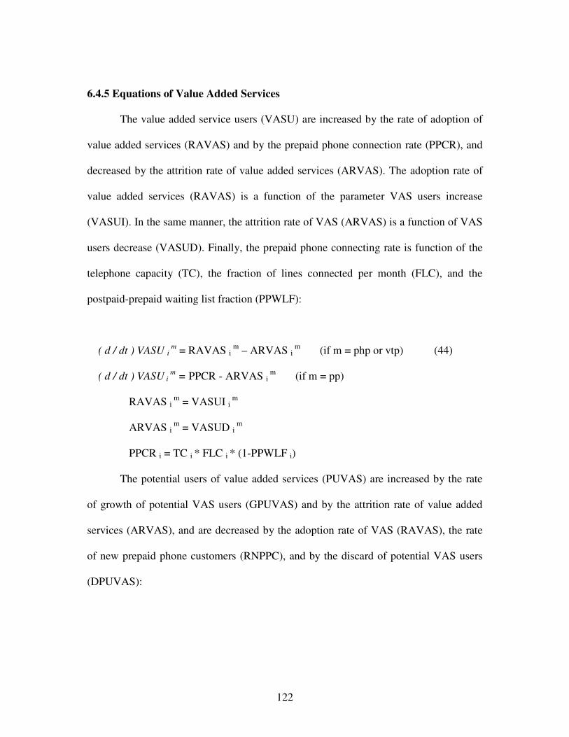
122

6.4.5 Equations of Value Added Services

The value added service users (VASU) are increased by the rate of adoption of

value added services (RAVAS) and by the prepaid phone connection rate (PPCR), and

decreased by the attrition rate of value added services (ARVAS). The adoption rate of

value added services (RAVAS) is a function of the parameter VAS users increase

(VASUI). In the same manner, the attrition rate of VAS (ARVAS) is a function of VAS

users decrease (VASUD). Finally, the prepaid phone connecting rate is function of the

telephone capacity (TC), the fraction of lines connected per month (FLC), and the

postpaid-prepaid waiting list fraction (PPWLF):

( d / dt ) VASU i m = RAVAS i m – ARVAS i m (if m = php or vtp) (44)

( d / dt ) VASU i m = PPCR - ARVAS i m (if m = pp)

RAVAS i m = VASUI i m

ARVAS i m = VASUD i m

PPCR i = TC i * FLC i * (1-PPWLF i)

The potential users of value added services (PUVAS) are increased by the rate

of growth of potential VAS users (GPUVAS) and by the attrition rate of value added

services (ARVAS), and are decreased by the adoption rate of VAS (RAVAS), the rate

of new prepaid phone customers (RNPPC), and by the discard of potential VAS users

(DPUVAS):

123

( d / dt ) PUVAS i m = GPUVAS i m + ARVAS i m – RAVAS i m - DPUVAS i m

(if m = php or vtp) (45)

( d / dt ) PUVAS i m = GPUVAS i m + ARVAS i m – RNPPC i - DPUVAS i m

(if m = pp)

The waiting list of prepaid phone subscribers (WLPP) is increased by the rate of

new prepaid phone customers (RNPPC) and decreased by the prepaid phone connection

rate (PPCR):

( d / dt )WLPP i = RNPPC i - PPCR i (46)

The rate of growth of potential VAS users (GPUVAS) for the case of payphones

(php) is function of the population growth (GPO) and the fraction of population able to

use calling cards (FPAUC), and GPUVAS for virtual telephony is the sum of the rate of

new postpaid customers (RNC) and the rate of new prepaid customers (RNPPC), which

are the flows of people interested in the telephone service but not connected yet.

Finally, the GPUVAS for prepaid phones is equal to the growth of the population of

telephone subscriber (GPTS):

GPUVAS i php = GPO i * FPAUC i (47)

GPUVAS i vtp = RNC i + RNPPC i

GPUVAS i pp = GPTS i

The discard of potential VAS users (DPUVAS) for payphones (php) is function

of the rate of new postpaid users (RNC) and the rate of new prepaid users (RNPPC).

124

The DPUVAS for virtual telephony (vtp) is a function of the rate of connecting postpaid

subscribers (CR) and the rate of connecting prepaid customers (PPCR). Finally, the

DPUVAS for prepaid phone (pp) is equal to the rate of people willing to pay the

monthly rental fee of the postpaid telephone service or new potential customer rate

(NPCR):

DPUVAS i php = RNC i + RNPPC i (48)

DPUVAS i vtp = CR i + PPCR i

DPUVAS i pp = NPCR i

The VAS users increase (VASUI) and VAS users decrease (VASUD) are a

function of the VAS users adjustment (VASUAD):

VASUI i m = VASUAD i m (if VASUAD i m > 0) (49)

VASUD i m = -VASUAD i m (if VASUAD i m < 0)

The VAS users adjustment (VASUAD) is a function of the indicated VAS users

(IUVAS), the actual VAS users (VASU), and the delay to adjust VAS users (DADUV).

VASUAD i m = (IUVAS i m - VASU i m) / DADUV (50)

The indicated users of value added services (IUVAS) are a function of the

maximum demand for a particular VAS (MAXDVAS) and the demand fraction of VAS

(DFVAS):

125

IUVAS i m = MAXDVAS i m * DFVAS i m (51)

The maximum demand of virtual telephony (vt), payphone (php), and prepaid

phone (pp) services (MAXDVAS) is function of the number of value added service

users (VASU), the potential VAS users (PUVAS), and the population of potential and

actual telephone subscribers (PTS):

MAXDVAS i m = VASU i m + PUVAS i m (if m = vt or php) (52)

MAXDVAS i m = PTS i (if m = pp)

The demand fraction of VAS (DFVAS) is function of the price fraction of VAS

(PFVAS), the availability of VAS fraction (AVASF), the easy to use of VAS factor

(EUVASF), and the network externality impact (NEI). The user interface of the

payphone service is a characteristic that indicates how easy is to handle a payphone

with a prepaid calling card. This will influence the efficient use and adoption of this

VAS (Thorner, 1994). The friendliness of this interface has been ranked from zero to

one, which indicates impossible and very easy to use respectively. The normal values

used in the model for the payphone easy to use factor are 0.7 for rural areas and one for

urban areas. On the other hand, the user interface of the virtual telephony service is a

characteristic that indicates how easy is to handle a payphone, a prepaid calling card,

and a mailbox together. The normal values used in the model for the virtual telephony

easy to use factor are 0.5 for rural areas and 0.7 for urban areas. Finally, the easy to use

factor value of the prepaid telephone service is assumed one. This indicates that the

prepaid calling card is very easy to handle:

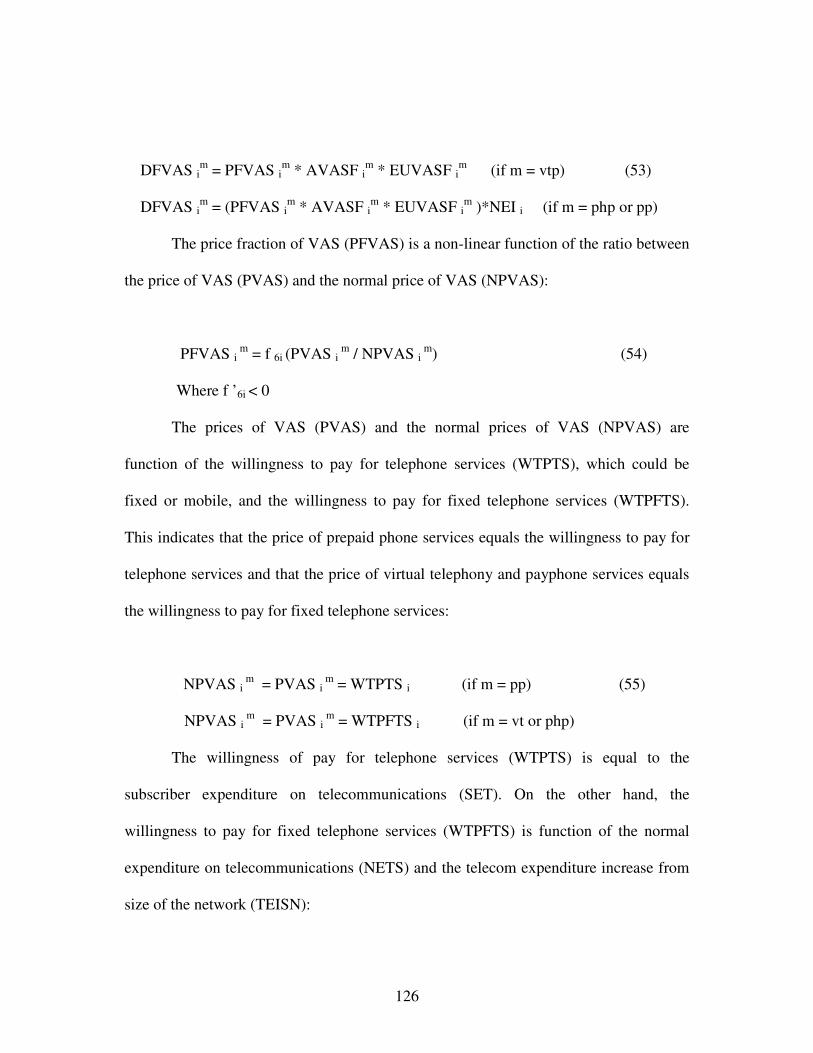
126

DFVAS im = PFVAS im * AVASF im * EUVASF im (if m = vtp) (53)

DFVAS im = (PFVAS im * AVASF im * EUVASF im )*NEI i (if m = php or pp)

The price fraction of VAS (PFVAS) is a non-linear function of the ratio between

the price of VAS (PVAS) and the normal price of VAS (NPVAS):

PFVAS i m = f 6i (PVAS i m / NPVAS i m) (54)

Where f ’6i < 0

The prices of VAS (PVAS) and the normal prices of VAS (NPVAS) are

function of the willingness to pay for telephone services (WTPTS), which could be

fixed or mobile, and the willingness to pay for fixed telephone services (WTPFTS).

This indicates that the price of prepaid phone services equals the willingness to pay for

telephone services and that the price of virtual telephony and payphone services equals

the willingness to pay for fixed telephone services:

NPVAS i m = PVAS i m = WTPTS i (if m = pp) (55)

NPVAS i m = PVAS i m = WTPFTS i (if m = vt or php)

The willingness of pay for telephone services (WTPTS) is equal to the

subscriber expenditure on telecommunications (SET). On the other hand, the

willingness to pay for fixed telephone services (WTPFTS) is function of the normal

expenditure on telecommunications (NETS) and the telecom expenditure increase from

size of the network (TEISN):

127

WTPTS i = SET i (56)

WTPFTS i = NETS i * TEISN i

The availability of VAS fraction (AVASF) for payphones (php) is function of

the infrastructure availability (IA) of payphone devices (phpd) and the infrastructure

availability (IA) of calling card numbers (ccn). The availability of VAS fraction

(AVASF) for virtual telephony is a function of the infrastructure availability (IA) of

mailboxes (mb), the infrastructure availability (IA) of payphone devices (phpd), and the

infrastructure availability (IA) of calling card numbers (ccn). Finally, the AVASF for

prepaid phones is a function of the infrastructure availability of calling card numbers

(ccn). The availability of payphone and virtual telephony services is mainly influenced

by the availability of payphone infrastructure. The superscript n refers to any type of

value added service infrastructure, mailboxes (mb), payphone devices (pphd), and

calling card numbers (ccn):

AVASF i php = IA i phpd * IA i ccn (57)

AVASF i vtp = IA i mb * IA i phpd * IA i ccn

AVASF i pp = IA i ccn

The infrastructure availability (IA) of payphone devices (pphd) is a function of the

payphone infrastructure installed (PAYII) , the population of the region (POP), and the

referential payphone device availability per person (RPA):

128

IA i pphd = (PAYII i / POP i ) / RPA (58)

The infrastructure availability (IA) of mailboxes and calling card numbers is

assumed one in the model, since the deployment delays and costs of each of these VAS

infrastructures are much lower than the deployment delay and cost of the payphone

infrastructure. This means that mailboxes and calling card numbers are always

considered available.

The referential payphone device availability per person (RPA) has a maximum

level of three payphones per 1000 people. This threshold is typical for developed

countries with a considerable penetration of payphones (World Telecommunication

Indicators Database, 2004).

The payphone devices infrastructure installed (PAYII) are increased by

payphone deployment rate (PAYDR) and decreased by payphone discard rate

(PAYDIR). The payphone deployment rate (PAYDR) is function of the payphone

deployment in progress (PAYDIP) and the payphone deployment delay (PAYDD). The

payphone discard rate is function of the payphone infrastructure installed (PAYII), the

payphone deployment in progress (PAYDIP), the desired payphone infrastructure

installed (DPAYII), and the delay to adjust payphone Infrastructure (DAPAYI):

( d / dt ) PAYII i = PAYDR i – PAYDIR i (59)

PAYDR i = PAYDIP i / PAYDD i

PAYDIR i = (PAYII i + PAYDIP i – DPAYII i ) / DAPAYI i

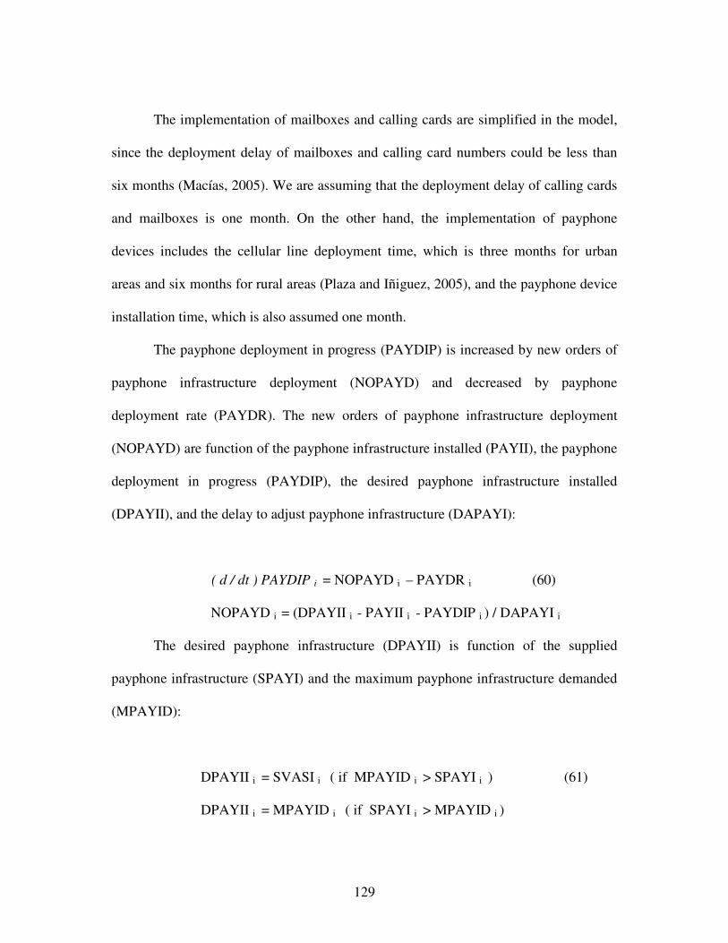
129

The implementation of mailboxes and calling cards are simplified in the model,

since the deployment delay of mailboxes and calling card numbers could be less than

six months (Macías, 2005). We are assuming that the deployment delay of calling cards

and mailboxes is one month. On the other hand, the implementation of payphone

devices includes the cellular line deployment time, which is three months for urban

areas and six months for rural areas (Plaza and Iñiguez, 2005), and the payphone device

installation time, which is also assumed one month.

The payphone deployment in progress (PAYDIP) is increased by new orders of

payphone infrastructure deployment (NOPAYD) and decreased by payphone

deployment rate (PAYDR). The new orders of payphone infrastructure deployment

(NOPAYD) are function of the payphone infrastructure installed (PAYII), the payphone

deployment in progress (PAYDIP), the desired payphone infrastructure installed

(DPAYII), and the delay to adjust payphone infrastructure (DAPAYI):

( d / dt ) PAYDIP i = NOPAYD i – PAYDR i (60)

NOPAYD i = (DPAYII i - PAYII i - PAYDIP i ) / DAPAYI i

The desired payphone infrastructure (DPAYII) is function of the supplied

payphone infrastructure (SPAYI) and the maximum payphone infrastructure demanded

(MPAYID):

DPAYII i = SVASI i ( if MPAYID i > SPAYI i ) (61)

DPAYII i = MPAYID i ( if SPAYI i > MPAYID i )

130

The cost of the payphone infrastructure or payphone device (CPAYI i) is the

sum of the cost of the payphone device (CPD) and the cost of telephone line (COT).

The cost of the payphone device is assumed 500 dollars, and the cost of a cellular

telephone line is assumed 200 dollars for urban areas and 300 dollars for rural areas

(Plaza and Iñiguez, 2005). The cost of payphone infrastructure is relatively high when

compared with the cost of calling cards and mailboxesThe cost of the payphone device

is assumed 500 dollars, and the cost of a cellular telephone line is assumed 200 dollars

for urban areas and 300 dollars for rural areas (Plaza and Iñiguez, 2005). The cost of

payphone infrastructure is relatively high when compared with the cost of calling cards

and mailboxes. The cost of a calling card number is five dollars and the cost of a

mailbox is ten dollars (Macías, 2005). :

CPAYI i = CPD + COT i (62)

The maximum infrastructure demanded for payphone devices (MPAYID i ) is a

function of the population (POP) and the referential payphone availability per person

(RPA):

MPAYID i = POP i * RPA (63)

The investment in payphone infrastructure (IPAYI) is a function of the total

allocated investment in payphones (TIPAY) and the fraction of investment in payphone

infrastructure (FIPAYI). The total investment in payphone (TIPAY) is a function of the

total potential investment (TPI) and the percentage of investment in value added service

131

(PIVAS). As described before, we are assuming that infrastructure availability (IA) of

mailboxes and calling card numbers is one. Therefore, the process of deployment of

mailboxes and calling card numbers can be simplified and the only VAS infrastructure

deployment process actually simulated in the model is the correspondent to payphone

infrastructure. For this reason, the percentage of investment in VAS (PIVAS) is equal to

the percentage of payphone investment, which is assumed 0.4 percent:

IPAYI i n = TIPAY * FIPAYI i n (64)

TIPAY = TPI * PIVAS

6.5 A Value Added Service Strategy for Improving Regional Telecommunications

The implementation of a prepaid phone service alone without any other VAS

implementation is observed at the top of Table 11 (VAS 1) and represents a referential

case for the following set of simulations that describe the VAS strategy. The strategy

will show the synergy that is generated when different value added services are

strategically combined and strengthen some key positive feedback loops of the system.

The strategy combines the individual impact that prepaid phone, virtual

telephony, and payphone services have on telephone expansion, which was described in

previous sections and are shown in Figures 17, 18, and 19. The implementation of a

prepaid phone service together with virtual telephony and payphone services uses the

same investment in payphones for the virtual telephony and payphone services

simultaneously. This makes costly payphones more productive since revenues from

132

virtual telephony and payphone phone calls are collected using the same payphone

infrastructure. It is important to note that the major portion of the investment required to

provide virtual telephony and payphone services is on the payphone infrastructure,

which is subtracted from the investment in telephone expansion, as observed in negative

feedback loops 16 and 21 of Figures 17 and 18 respectively.

The performance of this VAS strategy is observed in VAS 2 and VAS 3 of Table

11. The VAS 2 implementation has a low payphone investment of 0.4 percent of the

total investment budget. This improves the national and regional telephone density of

the country, with respect to the referential case. However, the rural-urban teledensity

gap is not improved in spite of the rural telephone density growth. For instance in year

15, the normalized rural telephone density is improved from its normalized value of

107.36 (VAS 1) to 284.90 (VAS 2), and the urban telephone density is improved from

97.082 (VAS 1) to 138.72 (VAS 2).

On the other hand, the VAS 3 implementation increases the payphone

investment from 0.4 to 4 percent. It is observed that the improvement on the level of

payphone infrastructure considerably increases the national and regional telephone

density of the country and increases the rural-urban telephone density ratio. For instance

in year 15, the rural telephone density increases to 2,270 (VAS 3), which is much higher

than 284.9 (VAS 2) and 107.36 (VAS 1). The urban telephone density increases to

162.49 (VAS 3), which is higher than 138.725 (VAS 2) and 97.082 (VAS 1). The rural-

urban telephone density ratio is increased to the normalized value of 16.67 (VAS 3),

which is much higher than the value of 1.11 observed in VAS 1 and VAS 2. This occurs

133

due to the combined action of positive feedback loops 13, 18, 19, 23, 24, 25, 26, 27, 28,

and 29 in Figures 17, 18, and 19, which strengthen the network externality impact in the

system. As described before, this improves the telephone service willingness to pay and

the prepaid and postpaid telephone demand, which expand the financial resources of the

telephone company and the total number of telephone lines.

This combination of services enhances the network externality impact by

expanding the number of people connected to the system. The network externality

improvement increases the willingness to pay for telephone services and the prepaid and

postpaid telephone demand. The improvement on the telephone service willingness to

pay expands the expenditure on prepaid virtual telephony, payphone, and telephone

services, as shown in Figures 17, 18, and 19. This situation increases the revenue and

financial resources of the telephone company, as seen in VAS 2 and VAS 3 of Table 11.

The enhanced prepaid and postpaid telephone demand improves the number of prepaid

and postpaid telephone subscribers in the network, as observed in positive feedback

loops 28 and 29 of Figure 19. This expands the financial resources of the telephone

company, as indicated in positive feedback loops 26 and 27.

The higher the number of payphones functioning in the region, the higher the

availability of payphone and virtual telephony services. This situation increases the

willingness to pay for these services, which improves their demand and adoption. The

growth of virtual telephony and payphone users expands the financial resources of the

telephone company, as observed in positive feedback loops 13 and 19 of Figures 17 and

18 respectively. The performance and behavior of the VAS implementations described

134

in this and previous sections are also observed in Figures 20 and 21, which show the

national teledensity and the rural-urban teledensity gap.

Table 11. Value Added Service Strategy for Improving Rural Telephony in

Developing Countries with a Cellular Access Network

VAS Telecom Indicators 0 5 9 15

1. Prepaid Phone Rural Tel. Density 1.000 7.636 15.455 107.364without any other Urban Tel. Density 1.000 7.722 15.150 97.082VAS National Tel. Density 1.000 7.995 16.147 107.880

Rural/Urban T D Ratio 1.000 1.111 1.111 1.111Financial Resources 1.000 0.189 0.616 8.492Prepaid/Postpaid Ratio 0 2.021 2.060 2.000

2. Prepaid Phone Rural Tel. Density 1.000 8.000 19.818 284.909,Virtual Telephony Urban Tel. Density 1.000 8.643 22.697 138.725, and Payphone Serv. National Tel. Density 1.000 8.935 24.129 156.313with Low Payphone Rural/Urban T D Ratio 1.000 1.111 1.111 1.111

Financial Resources 1.000 0.232 1.139 39.718Payphones/ 1000 people 0 0.048 0.123 1.688Prepaid/Postpaid Ratio 0 2.055 2.172 2.198

3. Prepaid Phone Rural Tel. Density 1.000 14.091 322.818 2270.000,Virtual Telephony Urban Tel. Density 1.000 31.360 162.493 162.493, and Payphone Serv. National Tel. Density 1.000 32.120 175.991 209.263with Higher Payphone Rural/Urban T D Ratio 1.000 0.370 2.222 16.667

Financial Resources 1.000 1.313 26.436 170.383Payphones/ 1000 people 0 0.742 2.203 3.000Prepaid/Postpaid Ratio 0 2.579 3.174 2.700

Years

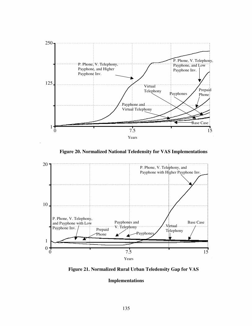
135

Base Case

Payphones

Virtual Telephony

Payphone and Virtual Telephony

Prepaid Phone

P. Phone, V. Telephony, Payphone, and Low Payphone Inv.

P. Phone, V. Telephony, Payphone, and Higher Payphone Inv.

0 7.5 15 Years

1

125

250

Figure 20. Normalized National Teledensity for VAS Implementations

P. Phone, V. Telephony, and Payphone with Higher Payphone Inv.

P. Phone, V. Telephony, and Payphone with Low Payphone Inv. Prepaid

Phone

Payphones and V. Telephony Virtual

Telephony

Base Case

Payphones

0 7.5 15 Years

1 0

10

20

Figure 21. Normalized Rural Urban Teledensity Gap for VAS

Implementations

136

6.6 Base Case Values


1. Monthly Rental Fee (Urban and Rural) $1 2. Urban Income per Capita $1708


4. Total Connected Subscribers Initial 50,000 5. Percent. Rural Lines 2.5%






12. Urban Cost per Line $200

13. Rural Cost per Line $300

14. Cost of each Mailbox $10

15. Cost of each C.Card Number $5

16. Cost of each Payphone Dev. $500

17. Telephone Deployment Time (Urban) 3 mo.

18. Telephone Deployment Time (Rural) 6 mo.

19. Percentage Payphone Investment 0%

20 Number of Telephones per Urban House 2





25. Easy to Use Factor Virtual Telephony (Urban) 0.7

26. Easy to Use Factor Virtual Telephony (Rural) 0.5

27. Easy to Use Factor Payphone (Urban) 1

137

28. Easy to Use Factor Payphone (Rural) 0.7

29. Easy to Use Factor Prepaid Phone 1

30. Referential Payphone Availability 0.003


32. License Cost $50 Millions













45. License Duration 15 years













138

58. Number of Payphone Users per House 2

59. Delay to Adjust VAS (Users) 3 mo.

60. Delay to Adjust Payphone Infrastructure 3 mo.

61. Payphone Devices Implementation Delay 1 mo.

62. Urban Investment Fraction (Payphone Infra) 0.965


64. VAS Investment referential 0

65. VAS Offered 0 Table 12. Base Case values of Value Added Services Analysis 6.7 Sensitivity Analysis of Value Added Service Strategy

Several experiments were conducted to test the sensitivity of the VAS strategy to

changes in the characteristics and costs of these value added services and different

perceptions of the population about them. The user interface of these services became

more complex and difficult to handle, then the easy to use factor of virtual telephony,

payphone, and prepaid phone services were considerably reduced. On the other hand,

the perception of the population about the availability of payphones in the region got

more stringent, and then the payphone availability referential was increased. Finally, the

investment in VAS infrastructure comes to be more costly, and then the cost of each

calling card, mailbox, and payphone was raised. The simulation results of the sensitivity

analysis are shown in Table 13.

The virtual telephony easy to use factor was reduced from 0.7 to 0.3 in urban

areas and from 0.5 to 0.15 in rural areas. The payphone easy to use factor was reduced

from one to 0.5 in urban areas and from 0.7 to 0.3 in rural areas. The cellular prepaid

phone easy to use factor was reduced from one to 0.5 in urban and rural areas. On the

139

other hand, the referential payphone availability was increased from three payphones

per 1000 people to five payphones per 1000 people. Finally, the cost of a calling card

number was increased from five to ten dollars, the cost of a telephone mailbox was

increased from ten to twenty dollars, and the cost of each payphone device was raised

from 500 to 800 dollars.

It is observed in VAS 2 and VAS 3 of Table 13 that the provision of prepaid

phone, virtual telephony, and payphone services together using a cellular network still

improve the national and regional telephone densities under this new scenario, in the

long term, with respect to the base case and the prepaid phone service implemented

alone, which is indicated in VAS 1. In addition, it is also observed in VAS 2 and VAS 3

that increasing the investment in payphone expansion from four to ten percent improve

the telephone densities and the rural-urban telephone density gap. However, this

sensitivity analysis also shows that the rural-urban telephone density gap is not

improved with respect to the base case, in spite of an important growth in telephone

densities and financial resources. Therefore, it is important to emphasize that the

positive impact of VAS described in previous sections depends mainly on the

friendliness of the user interface or easy to use factor and the availability or easy to

acquire of these services in the region. The better the user interface and more reachable

are these value added services in the country, the higher the improvement that this VAS

implementation is able to produce in the regional telecom system.

140

Table 13. Value Added Service Strategy for Improving Rural Telephony in

Developing Countries with a Higher VAS Infrastructure Costs and Payphone

Availability Referential, and Lower VAS Easy to Use Factor.

VAS Telecom Indicators 0 5 9 15

Base Run Rural Tel. Density 1.000 11.000 14.545 33.455Urban Tel. Density 1.000 6.292 9.501 25.592National Tel. Density 1.000 6.599 10.212 28.525Rural/Urban T D Ratio 1.000 1.852 1.852 1.481Financial Resources 1.000 0.099 0.223 1.320

1. Prepaid Rural Tel. Density 1.000 7.455 14.091 77.909Phone, without Urban Tel. Density 1.000 7.462 13.671 70.198any other VAS National Tel. Density 1.000 7.724 14.571 78.018

Rural/Urban T D Ratio 1.000 1.111 1.111 1.111Financial Resources 1.000 0.167 0.482 5.662

2. Prepaid Rural Tel. Density 1.000 6.727 12.727 98.273Phone, Virtual Urban Tel. Density 1.000 6.853 13.538 98.244Telephony, and National Tel. Density 1.000 7.092 14.410 108.986Payphone Serv. Rural/Urban T D Ratio 1.000 1.111 1.111 1.1114% Payphone Inv. Financial Resources 1.000 0.140 0.465 7.824

Payphones/ 1000 people 0.000 0.275 0.536 3.405

3. Prepaid Rural Tel. Density 1.000 5.727 10.818 130.000Phone, Virtual Urban Tel. Density 1.000 6.088 12.688 106.232Telephony, and National Tel. Density 1.000 6.295 13.484 118.249Payphone Serv.& Rural/Urban T D Ratio 1.000 1.111 1.111 1.48110% Payphone Financial Resources 1.000 0.107 0.398 9.579Investment Payphones/ 1000 people 0.000 0.572 1.093 3.663

Years

141

6.8 Conclusions

This chapter presents an investigation of value added services on the expansion

of telephone capacity in developing countries. It was found that a strategic

implementation of value added services are able to accomplish the purpose of

improving the telephone penetration in the country. The implementation of these value

added services in isolation moderately improved the number of telephone lines.

However, it proved that prepaid phone, virtual telephony, and payphone services, which

are innovative services over the telephone network, are able to considerably improve

the financial resources of the telephone company and accelerate the dispersion of

telephone lines in rural areas of developing countries, only when implemented together.

The prepaid phone service pricing mechanism is based on the willingness to pay

of the subscribers. The combination of virtual telephony with prepaid phone service

reinforces the impact of network externality on the system, which increases the

willingness to pay and revenue of the telephone service per subscriber. The addition of

the payphone service to the previous combination improves the revenue and financial

resources of the telephone company, which are used for telephone expansion and value

added service implementation. Finally, the easy to use and easy to acquire of these

value added services are important characteristics that need to be constantly improved

in order to be able to reach the important growth in telephone penetration observed in

this study.

142

Chapter 7. An Analysis of Wireless Technologies on the Regional Dispersion of

Telephone Services in Developing Countries.

7.1 Introduction

The access plant of the traditional telephone network, as opposed to the switches

and backhaul connections, is extremely unproductive and underutilized, and shows

fewer economies of scales since it is largely dedicated. The access plant is considered

the largest asset of the telephone network, since this can account for more than half of

the total assets of the company. The traditional access plant is wired, and is largely a

function of the distance from the subscriber to central office or switching equipment.

For this reason, the cost to provide a telephone line to a rural subscriber could be ten

times the cost for an urban subscriber (Calhoun,1992).

Wireless technologies, such as cellular networks and Wireless Local Loop

(WLL), are being seen as a way to increase telephone density in developing countries,

due to its rapid deployment and lower cost (Noerpel, 1997). The cellular networks have

grown rapidly in developing countries in recent years, especially in cities and other

urban areas. The wireless technologies are less sensitive to distance than traditional

wired technologies, which makes them more attractive for deployment in dispersed or

scattered rural environments. However, there are still several questions regarding their

viability in developing countries. For instance, the lack of electricity and reliable power

supply has been considered the biggest challenge in deploying wireless systems in rural

areas (Rycroft, 1998).

143

Due to the high cost of subscriber equipment and quality problems, the

implementation of of WLL services in developing countries has been limited (Robledo

and Arathoon, 2002). My investigation showed, however, that WLL could be a viable

alternative, especially in low-density areas, where the cost of wired systems increases

considerably and the large coverage and low deployment delay of WLL systems

become significant determinants of dispersion of telephone services.

Cellular systems are considered the best technology currently in the market that

is able to accelerate the growth of telephone services in developing countries for urban

areas. However, it was found that in thinly populated rural areas, WLL performs better

than any other access technology including cellular systems. In this scenario, the

cellular access network still performs better than the conventional wired telephone

network.

7.2 Impact of Access Technologies on Telephone Expansion

The wired access plant is the largest component of a conventional telephone

network, since the cost of the backhaul connections and switches are considered

insignificant when compared with the cost of the access component (Webb, 2000).

Figure 22 shows a schematic of the wired telephone network, which includes the wired

local loop, the switching office also known as central office or local exchange, and the

backhaul connections. The wired local loop connects the switching office to the

subscriber, and the backhaul connections interconnect the switching offices. The wired

access plant, which goes from the switching office to the subscriber, includes the local

144

loops associated with access and can account for more than fifty percent of the book

assets of the telephone company.

Figure 22. Schematic of a Wired Telephone Network

It has been observed that the costs of wired local loops increases at a greater

than linear rate as a function of the distance, and decreases as the subscriber density

increases (Calhoun, 1992; Mannisto and Tuisku, 1994; Webb, 2000). This situation

occurs because longer wired loops require more cable, and also the additional loading

coils and larger gauge cable. Historically, the telecom implementation has started in

more dense urban areas, and then it has moved toward less dense suburban or rural

areas, which have represented a transition to lower economies of scale, longer loop

distances, and higher deployment costs (Saunders et. al., 1994). In rural areas, where the

population density is very low, the cost of the wired local loop could be more than ten

times the cost in urban areas (Calhoun, 1992).

The wireless technologies are seen as an alternative to the access plant, which

can replace the dedicated and underutilized copper wire with a shared and more

145

efficient radio spectrum among subscribers (Duckworth, 2004). Figure 23 shows the

schematic of a telephone network with a wireless access plant, where the wired local

loop of a conventional telephone network has been replaced with a wireless link, which

can be fixed for the case of Wireless Local Loop systems or mobile for the case of

cellular systems. The cost of wireless systems has less sensitivity to distance and

subscriber density than wired systems, since it has little impact where the subscribers

are located inside the area of coverage of the radio cell. However, it is important to

emphasize that there could be some extra costs associated with very remote subscribers

living in fringe coverage zones, where it may be necessary to install a higher subscriber

antenna with higher gain (Calhoun, 1992).

Figure 23. Schematic of a Telephone Network with Wireless Access Plant

The wireless technologies, such as cellular and WLL, have been considered to

have the potential to increase telephone density in developing countries, because of its

rapid deployment and lower implementation costs (Noerpel, 1997; Hamersma, 1996). In

addition, wireless systems are supposed to reduce the relative cost difference between

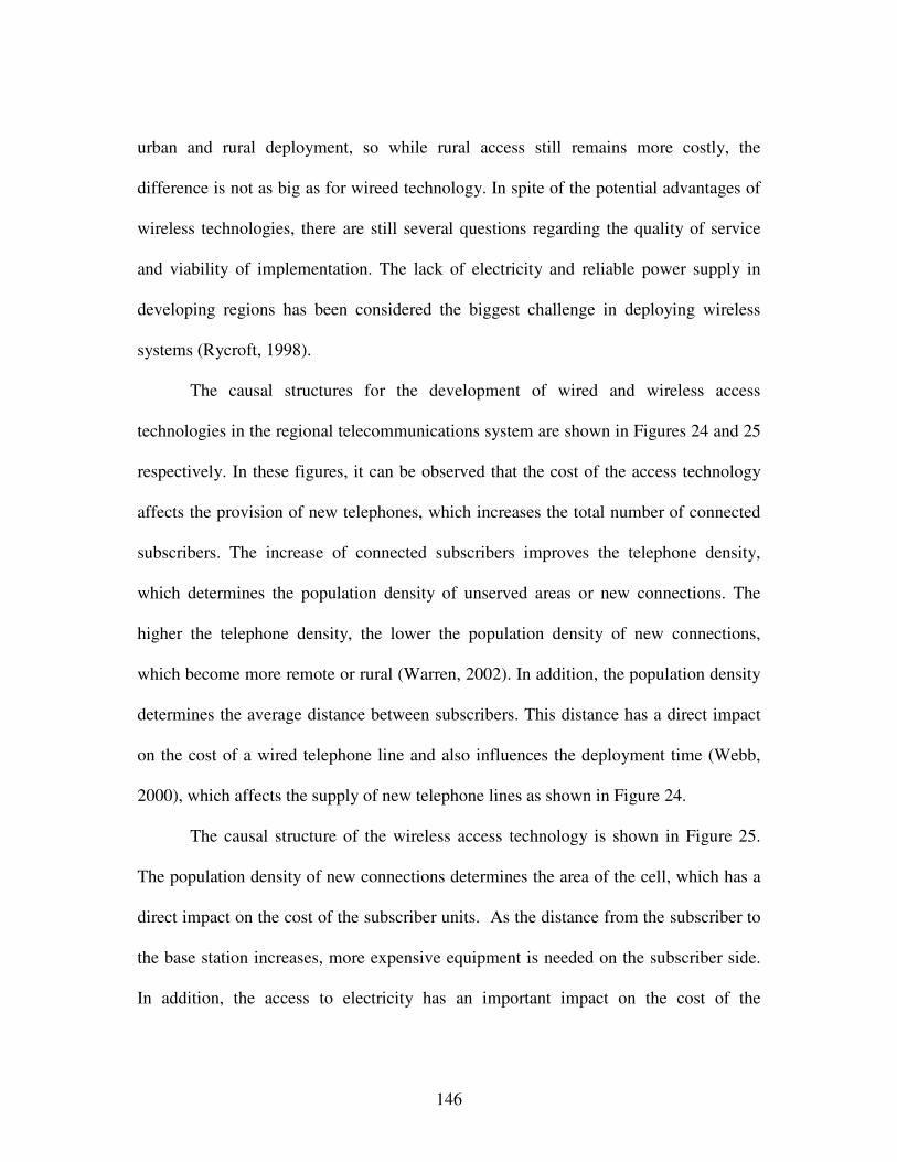
146

urban and rural deployment, so while rural access still remains more costly, the

difference is not as big as for wireed technology. In spite of the potential advantages of

wireless technologies, there are still several questions regarding the quality of service

and viability of implementation. The lack of electricity and reliable power supply in

developing regions has been considered the biggest challenge in deploying wireless

systems (Rycroft, 1998).

The causal structures for the development of wired and wireless access

technologies in the regional telecommunications system are shown in Figures 24 and 25

respectively. In these figures, it can be observed that the cost of the access technology

affects the provision of new telephones, which increases the total number of connected

subscribers. The increase of connected subscribers improves the telephone density,

which determines the population density of unserved areas or new connections. The

higher the telephone density, the lower the population density of new connections,

which become more remote or rural (Warren, 2002). In addition, the population density

determines the average distance between subscribers. This distance has a direct impact

on the cost of a wired telephone line and also influences the deployment time (Webb,

2000), which affects the supply of new telephone lines as shown in Figure 24.

The causal structure of the wireless access technology is shown in Figure 25.

The population density of new connections determines the area of the cell, which has a

direct impact on the cost of the subscriber units. As the distance from the subscriber to

the base station increases, more expensive equipment is needed on the subscriber side.

In addition, the access to electricity has an important impact on the cost of the

147

subscriber unit. Also, additional power supplies, like solar panels or batteries, might be

required, which further escalates costs. The population density of new connections

determines the number of subscribers per base station, which influences the cost of a

base station per subscriber. The higher the cost of the base station per subscriber and

subscriber equipment, the higher the deployment cost of a wireless telephone in the

system.

Figure 24. Causal Structure of Wired Technology in the Regional

Telecommunications System


TelephoneDensity

Population Density ofNew Connections

Cost per WiredLineAdditional

Telephone Lines-

+

+

-

DeploymentDelay

-

Distance C.Office-Households

-

+

+

-31

-30

148

Figure 25. Causal Structure of Wireless Technologies in the Regional

Telecommunications Systems

7.3 Access Technologies Formulation

7.3.1 Equations of Wired Access Network

The cost of the wired network per line (CWIRE) is the sum of the cost of

external plant per line (CEXTP) and the cost of the core network per line (CCORE),

which includes the switching office and backhaul connection costs. Subscript i refers to

any of the two regions, urban (u) and rural (r):

CWIRE i = CEXTP i + CCORE i (65)


Te lephoneDensity

Population Density ofNew Connections

Subscribers perBase Station

Cost of a BaseStation perSubscriber

Cost perWire less Line

AdditionalTe lephone Lines

Households OutsideNormal Area of the

Cell

Subscriber UnitCosts

+

-

+-

+

+

-

-

+

+Access toElectricity

-

DeploymentDelay-

Mobility-

TelecomInvestment

+

Traffic+

+

Normal Radius ofB. Station

-

-32

-33

-34

149

The cost of the external plant per line (CEXTP) is function of the average

distance from the central office to the households (ADCTH), the cost per meter of cable

(CMC), and a referential base cost (RBC), which is considered to be about $ 150

(Kayani and Dymond 1997):

CEXTP i = RBC + (ADCTH i * CMC) (66)

The average distance from the central office to the households (ADCTH) is

function of the area of coverage of the central office (ARCCO), which assumes a

circular shaped area. The area of coverage of the central office is function of the number

of telephone lines per central office (NTLCO) and the number of telephone lines per

area (NLPA):

ADCTH i = SQRT(ARCCO i / 2*3.1416) (67)

ARCCO i = NTLCO / NLPA

The number of lines per area (NLPA) is function of the normal number of lines

per area (NNLPA) and the telephone lines-telephone density adequacy (TLTDA). The

telephone lines-telephone density adequacy (TLTDA) is a non-linear function of the

wired network telephone density (WNTD):

NLPA i = NNLPA i * TLTDA i (68)

TLTDA i = f 7i (WNTD i) Where f ’7i < 0

150

The normal number of lines per area (NNLPA) is function of the population

density (POPD) and the number of people per line (NUMPL), which depends on the

number of lines per house (NUMLH) and the number of people per house (NUMPH):

NNLPA i = POPD i / NUMPL i (69)

NUMPL i = NUMPH i / NUMLH i

The time to deploy a wired telephone line (TDWDL) is function of the time to

install the switching equipment (TISW), the external plant deployment time (DTEXP),

and the time to couple the external plant with the switching equipment (TCXPSW):

TDWDL i = TISW i + DTEXP i + TCXPSW i (70)

The external plant deployment time (DTEXP) is function of the referential

external plant deployment time (REXPDT) and the distance from the central office to

the household ratio (DCOHR). It has been assumed that laying a external plant in a

developing country with an urban population density of 284 people per square

kilometers takes about one year:

DTEXP i = REXPDT i * DCOHR i (71)

The distance from the central office to the household ratio (DCOHR) is function

of the average distance from the central office to the households (ADCTH) and a

referential distance from the central office to the households (RDCTH):

151

DCOHR i = ADCTH i / RDCTH i (72)

7.3.2 Equations of Wireless Access Networks

The cost of a wireless telephone line (CWLH), which includes cellular and

wireless local loop systems, is the sum of the cost of the base stations per line (CBSL),

the cost of the core network per line (CCNL), and the cost of the subscriber stations per

line (CSSL):

CWLH i = CBSL i + CCNL i + CSSL i (73)

The cost of the base stations per line (CBSL) is equal to the cost of a base station

(CABS) divided by the number of wireless lines per base station (WLBS):

CBSL i = CABS / WLBS i (74)

The number of wireless lines per base station (WLBS) is a function of the area

of the cell covered by the base station (ACBS), the number of wireless lines per area

(NLA), the area of the cell indicated (ACBSI), the maximum area of the cell (MARC),

and the maximum number of wireless lines per base station (MWLBS). The maximum

area of the cell assumes a circular cell and is function of the maximum radius of the

base station (MRAD). The area of the cell indicated (ACBSI) is function of the

maximum number of wireless lines per base station (MXWLBS) and the number of

wireless lines per area (NLA):

152

WLBS i = ARC * NLA i (If ACBSI i >= MARC) (75)

WLBS i = MWLBS i (If ACBSI i < MARC)

MARC = π * (MRAD)2

ACBSI i = MXWLBS i * NLA i

The area of the cell (ARC) is function of the maximum area of the cell (MARC)

and the area of the cell indicated (ACBSI):

ARC i = MARC (If ACBSI i >= MARC) (76)

ARC i = ACBSI i (If ACBSI i < MARC)

The cost of the subscriber stations per line (CSSL) is equal to the total cost of

the subscriber equipment inside a base station (TCSEBS) divided by the number of

wireless lines per base station (WLBS):

CSSL i = TCSEBS i / WLBS i (77)

The total cost of the subscriber equipment inside a base station (TCSEBS) is the

sum of the total cost of special subscriber equipment in a base station (TCSPSE), the

total cost of normal subscriber equipment in a base station (TCNSE), and the cost of

extra power supply for subscriber units without access to electricity (CPS):

TCSEBS i = TCSPSE i + TCNSE i + CPS i (78)

The total cost of special subscriber equipment in a base station (TCSPSE) is

equal to the cost of special subscriber equipment (CSPSE) multiplied by the number of

153

wireless phones outside the normal area of a cell (WPONAC). The total cost of normal

subscriber equipment in a base station (TCNSE) is equal to the cost of normal

subscriber equipment (CNSE) multiplied by the number of wireless phones inside the

normal area of a cell (WPINAC):

TCSPSE i = CSPSE * WPONAC i (79)

TCNSE i = CNSE * WPINAC i

The number of wireless phones outside the normal area of the cell (WPONAC)

is function of the number of wireless lines per area (NLA), the area of the cell (ARC),

and the normal area of the cell (NARC). The number of wireless phones inside the

normal area of the cell (WPINAC) is function of number of wireless lines per base

station (WLBS) and the number of wireless phones outside the normal area of the cell

(WPONAC). The normal area of the cell is a function of the normal radius of the base

station (NRAD):

WPONAC i = NLA i * (ARC i - NARC i) (If ARC i > NARC i) (80)

WPONAC i = 0 (If ARC i <= NARC i)

WPINAC i = WLBS i - WPONAC i

NARC i = π * (NRAD)2

The cost of power supply of subscriber units without access to electricity in a

base station (CPS) is function of the number of wireless phones per base station

154

(WLBS), the percentage of wireless phones without access to electricity (PWPWE), and

the cost of each solar panel equipment per subscriber (CESPE):

CPS i = WLBS i * PWPWE i * CESPE (81)

The wireless phones outside the normal area of the cell in a wireless network

require especial equipment in order to be able to connect to the base station.

Additionally, the households with cellular phones outside the normal area of the cell

will have their cellular equipment fixed or attached to the wall, which means a lack of

mobility. For this reason, a higher number of households located outside the normal

area of the cell translate into less mobility of the cellular system. In other words, the

higher the number of households inside the normal area of the cell, the higher the

mobility of the subscribers in the cellular network.

The average number of wireless phones inside the normal area of the cell

(AWPINAC) and the average number of wireless phones per base station (AWLBS)

determine the fraction of wireless phones in a base station with mobility (FWPWM).

The AWPINAC and AWLBS are first order exponential averages of the number of

wireless phones inside the normal area of the cell (WPINAC) and the number of

wireless phones per base station (WLBS) respectively. These averaging processes use

the time constant T2 and �1 is the first order exponential average:

FWPWM i = AWPINAC i / AWLBS i (82)

AWPINAC i = �1 [WPINAC i, T2]

155

AWLBS i = �1 [WLBS i, T2]

The fraction of mobile users in the system (FMUS) is a function of the postpaid

connected subscribers (CS), the prepaid telephone subscribers (VASU i pp), the total

wireless subscribers (WSUB), and the fraction of wireless phones in a base station with

mobility (FWPWM):

FMUS i = WSUB i * FWPWM i /(CS i + VASU i pp ) (83)

The total wireless subscribers (WSUB) is function of the postpaid service

connecting rate (CR), the prepaid service connecting rate (PPCR), the postpaid service

attrition rate (AR), and the prepaid service attrition rate (ARVAS i pp):

( d / dt ) WSUB i = CR + PPCR - AR - ARVAS i pp (84)

7.4 Telephone Dispersion for Different Access Networks

In this section, I simulate the historical and future behavior of the growth of the

cellular (Cellular #1) and conventional wired telephone networks in Ecuador, which is

shown in Figures 26, 27, 28, 29, 30, and 31. In addition, two hypothetical cases, which

consist on the implementation of Wireless Local Loop (WLL) and cellular networks

(Cellular #2) by the telephone operator as a replacement of the wired access network in

year 1993, are also simulated.

The simulations are calibrated for the case of Ecuador, which has an urban

income per capita of 1,708 dollars and a rural income per capita of 310 dollars. In

156

addition, its urban population density is 284 people per square kilometer and its rural

population density is nineteen people per square kilometer (World Development

Indicators, 2002). In Figure 26, it is possible to observe the moment when the number

of cellular phones surpassed the number of conventional telephone lines in year 2002. It

is important to note that most of the implementation of the cellular network has been in

urban regions.

The implementation of cellular systems in urban and rural areas involves the

deployment of base stations that have a normal radius of coverage of five kilometers

and an extended radius of coverage of thirty kilometers. The maximum number of

subscribers supported by each base station is 5,000. The normal cost of each cellular

base station is 150,000 dollars. In addition, the cost of a normal subscriber unit is fifty

dollars, and the cost of a special subscriber unit, which is used outside the normal

coverage of the base station, is 400 dollars. The normal subscriber unit is mobile since it

can move inside the normal area covered by a base station, but the especial subscriber

unit is fixed since it requires a special antenna attached to the wall of the house in order

to communicate with the base station. The access to electricity in urban areas is ninety

eight percent and in rural areas is fifty percent of the population. The cost of a solar

panel, which is used to supply with electricity the subscriber equipment in each house

without electricity, is 500 dollars. The license fee for cellular systems is assumed

50,000,000 dollars for a license period of fifteen years.

The implementation of WLL is similar to the cellular implementation. It

considers the same level of access to electricity and the use of the same solar panels as

157

the cellular case. It involves the deployment of base stations, which have a normal

radius of coverage of fifteen kilometers and an extended coverage of thirty-five

kilometers. The maximum number of users supported by each base station is 5,000

households. The normal cost of each base station is 150,000 dollars; the cost of a

normal subscriber unit is 400 dollars, and the cost of a special subscriber unit, which is

used outside the normal coverage of the base station, is 600 dollars. The license fee for

Wireless Local Loop has been set to 5,000,000 dollars for a license period of fifteen

years.

The deployment of the cellular network has produced the fastest growth of

telephones in urban and rural areas. It is observed in Figure 26 that the cellular network

increased exponentially in urban areas, which represents the historical behavior

observed in past years. The number of cellular subscribers keeps increasing

exponentially until they achieve steady state growth, which is indicated by a linear

growth. This situation is also observed in the hypothetical case in urban areas where the

telecom operator decides to replace the wired access network by a cellular access

network, as shown in Figure 26. The exponential growth of cellular phones is also

observed in rural areas.

The number of urban and rural telephones is considerably improved by the

implementation of the cellular network because it has the lowest cost per telephone and

the lowest deployment delay in both regions, as observed in Figures 28, 30, 29, and 31.

The improvement in the cost per telephone occurred in spite of the lack of electricity in

rural areas, which increases the cost of the cellular subscriber equipment due to the need

158

of solar panels. In addition, the low rural population density requires the use of more

expensive subscriber equipment, which is fixed to each house. Therefore, the

improvement on the telephone deployment costs and implementation delays observed in

cellular networks increase considerably the supply of urban and rural telephones, which

increase the revenue and financial resources of the telecom company.

When the cellular system is implemented in the regional telecom system, the

cellular subscribers increase the telephone density of the whole region. The higher the

telephone density, the lower the population density of the new connected subscribers as

shown by negative feedback loop 34 in Figure 25. The reduction of the population

density of the new connected subscribers because of the growth of the telephone density

increases the number of subscribers outside the normal area covered by a cellular base

station, as shown by negative feedback loop 33 in Figure 25. This determines a higher

number of subscribers requiring fixed antennas and especial equipment in order to

connect to the base stations from home, which represents higher costs for the subscriber

units. In addition, the low access to electricity is a major factor influencing the cost of

the subscriber unit, which increases the cost of deploying a phone in the system.

The higher the number of subscribers with fixed antennas located outside the

normal area covered by the base stations, the lower the number of subscribers with

mobility in the cellular network, as shown by negative feedback loop 32 in Figure 25.

The mobility and portability are characteristics of the cellular network that tend to

increase the traffic of the network since the willingness to pay and usefulness of a

telephone has been improved. This is also shown in negative feedback loop 32.

159

It is observed in Figure 27 that the hypothetical implementation of WLL slightly

improves the number of rural telephone lines in the long run with respect to the

conventional wired access network. This situation occurs because of the lower cost and

lower implementation delay of the WLL system with respect to the conventional wired

technology in rural areas, which is shown in Figures 29 and 31.

When the WLL technology is implemented in the regional telecom system, the

new WLL subscribers increase the telephone density of the region. The higher the

telephone density, the lower the population density of the new subscribers being

connected which is shown by negative feedback loop 34 in Figure 25. In addition, the

low access to electricity in developing countries is a major factor influencing the cost of

the subscriber unit, as shown in negative feedback loop 33 of Figure 25. The higher the

subscriber cost, the higher the cost of a WLL telephone line.

The growth of telephone lines in the conventional wired network also reduces

the population density of the new connected subscribers as the telephone density of the

region increases. This situation increases the distance between households as shown by

negative feedback loop 30 in Figure 24, which considerably increases the deployment

delay and the cost of a wired telephone line. The relatively high deployment delay and

cost of a wired telephone line reduces the supply of new telephone lines and the number

of connected households, as shown in negative feedback loops 30 and 31 of Figure 24.

This behavior can also be observed in Table 14.

160

WLL

Wired Cellular #1

Cellular #2

0

2,500,000

5,000,000

1993

1998

2003

2008

2014

Years

Phon

es

Figure 26. Urban Phones for Different Access Networks

WLL

Wired

Cellular #1

Cellular #2

1993 1998 2003 2008 2014 Years

0

300,000

600,000

Phon

es

Figure 27. Rural Phones for Different Access Networks

161

WLL Wired

Cellular #1 Cellular #2

1993 1998 2003 2008 2014 Years

0

250

500 D

olla

rs

Figure 28. Urban Cost for Different Access Networks

WLL Wired

Cellular #1

Cellular #2

500

650

800

1993 1998 2003 2008 2014 Years

Dol

lars

Figure 29. Rural Cost for Different Access Networks

162

WLL

Wired

Cellular #1

Cellular #2

1993 1998 2003 2008 2014 Years

0

7

14 M

onth

s

Figure 30. Urban Delay for Different Access Networks

WLL

Wired

Cellular #1 Cellular #2

1993

1998

2003

2008

2014

Years

0

12

24

Mon

ths

Figure 31. Rural Delay for Different Access Networks

163

Table 14. Performance of Different Access Technologies

Technology Telecom Indicators 1993 2003 2014

1. Cellular #1 Urban Phones (Phones) 0 1,656,907 4,338,018Rural Phones (Phones) 0 19,192 465,241Urban Cost (Dollars) 130 130 130Rural Cost (Dollars) 589 591 657Urban Delay (Months) 6 6 6Rural Delay (Months) 8 8 8

2. Wired Urban Phones (Phones) 538,418 1,529,822 2,280,357Rural Phones (Phones) 59,829 71,814 170,910Urban Cost (Dollars) 376 477 498Rural Cost (Dollars) 777 778 799Urban Delay (Months) 9 11 12Rural Delay (Months) 22 22 23

3. WLL Urban Phones (Phones) 538,418 1,220,959 2,299,933Rural Phones (Phones) 59,829 73,456 193,268Urban Cost (Dollars) 480 480 480Rural Cost (Dollars) 720 720 720Urban Delay (Months) 6 6 6Rural Delay (Months) 8 8 8

4. Cellular #2 Urban Phones (Phones) 538,418 3,027,613 4,592,831Rural Phones (Phones) 59,829 262,337 539,896Urban Cost (Dollars) 130 130 130Rural Cost (Dollars) 589 606 658Urban Delay (Months) 6 6 6Rural Delay (Months) 8 8 8

Years

164

7.5 Base Case Values


1. Monthly Rental Fee (Urban and Rural) $1 2. Urban Income per Capita $1708


4. Total Connected Subscribers Initial 598,287 5. Percent. Rural Lines 1 %






12. Number of Telephones per Urban House 1






18. License Cost $ 0











165



31. License Duration 15 years














45. Cost of the Core Network per Line $ 40

46. Time to Install Switching Equipment (Urban) 8 mo.

47. Time to Install Switching Equipment (Rural) 18 mo.

48. Time to Couple Ext. Plant with Switch. Equip. 1 mo.

49. Referential Ext. Plant Deployment Time 12 mo.

50. Referential Population Density 284

51. Number of Lines per Central Office 5,000

52. Referential Cost of External Plant $ 150

53. Population Density (Urban) 284

54. Population Density (Rural) 19

55. Referential Cost per Meter of Cable $ 0.1

56. Cost of Base Station $ 150,000

57. Cost of Solar Panel $ 500

58. Cost of Normal Subscriber Unit $ 50

166

59. Cost of Special Subscriber Unit $ 400

60. Access to Electricity (Urban) 0.98

61. Access to Electricity (Rural) 0.5

62. Maximum Radio of the Cell 30 km

63. Normal Radio of the Cell 5 k5

64. Maximum Wireless Lines per Base Station 5,000 Table 15. Base Case values of the Access Technologies Analysis

7.6 Sensitivity Analysis of Different Access Technologies

The preceding section showed how cellular technologies were able to

considerably improve the number of telephones in urban and rural areas of Ecuador.

New experiments were conducted to test the sensitivity of the cellular system and other

access technologies to changes in population densities. The population densities were

reduced from 284 people per square kilometer to seventeen people per square kilometer

in urban areas, and from nineteen people per square kilometer to two people per square

kilometer in rural areas. The simulation results of the sensitivity analysis are shown in

Table 16.

It is observed that a lower population density reduces the impact of the cellular

technology in the regional telecom system, but this technology is still able to increase

the number of phones in urban and rural areas when compared with the conventional

wired technology. This situation is observed in the hypothetical case when the cellular

access network is implemented as a replacement of the wired external plant, which is

indicated by technologies 1 and 4 in Table 16. However, it is observed that WLL

167

provides the best performance in urban and rural regions under this new scenario. This

happens due to the larger coverage of the WLL cell with respect to the cellular cell,

which reduces the cost. The larger radio of coverage per base station requires a lower

number of special and more expensive equipment required to connect the subscriber

with the base station in areas outside the normal coverage. It is also observed that the

cellular system improves the number of urban telephone lines in the very long run, for

its hypothetical case.

168

Technology Telecom Indicators 1993 1998 2003 2008 2014

1. Cellular #1 Urban Phones 0 86,675 111,651 162,828 276,715Rural Phones 0 965 1,231 1,777 2,999Urban Cost 246 249 249 250 252Rural Cost 706 706 706 706 706Urban Delay 6 6 6 6 6Rural Delay 8 8 8 8 8

2. Wired Urban Phones 538,458 548,448 548,784 548,940 549,013Rural Phones 59,829 56,236 46,142 33,420 21,671Urban Cost 648 606 569 546 530Rural Cost 1,338 1,335 1,329 1,322 1,316Urban Delay 91 85 78 76 74Rural Delay 195 194 193 192 191

3. WLL Urban Phones 538,458 776,121 1,307,627 1,602,804 1,809,448Rural Phones 59,829 63,860 73,048 112,214 181,203Urban Cost 480 480 519 531 531Rural Cost 853 853 854 856 862Urban Delay 6 6 6 6 6Rural Delay 8 8 8 8 8

4. Cellular #2 Urban Phones 538,458 733,486 1,011,228 1,543,091 2,586,728Rural Phones 59,829 62,128 65,512 72,481 88,396Urban Cost 272 280 295 329 387Rural Cost 707 707 707 707 707Urban Delay 6 6 6 6 6Rural Delay 8 8 8 8 8

Years

Table 16. Performance of Different Access Technologies for a Thinly Populated

Country

The reduction in the population densities increased the operating costs and

deployment delays of the telephone company for wireless and wired access network

technologies. However, the sensitivity analysis of the equipment, material, and labor

costs used in this investigation are left for future research.

169

7.7 Conclusions

This chapter presents an investigation about the use of three different access

technologies: wired access networks, Wireless Local Loop, and cellular systems. The

wireless technologies were able to considerably improve the regional dispersion of

telephone services.

There is no specific access technology that provides the best performance for

every type of environment. For instance, Wireless Local Loop was found the best

technology for improving the number of urban and rural telephones in a thinly

populated country. On the other hand, the cellular system implementation showed the

best performance for the specific case of Ecuador because of the lower deployment

delays and lower implementation costs in both urban and rural regions.

It is important to note that developing countries have experienced a low level of

implementation of Wireless Local Loop services in past years. However, this

investigation found that WLL could be a viable alternative in spite of its relative high

cost, especially in low-density countries, where the cost of wired systems increases and

the low deployment delay and relatively large coverage of WLL systems become

crucial factors on the dispersion of telephone services.

An important aspect observed in the analysis of this investigation was the impact

of deployment delay on the dispersion of telephone services. It was observed to be a

very important factor for increasing the number of telephone lines in developing

countries.

170

Chapter 8. Research Contribution and Conclusion

8.1 Practical Applications

This dissertation has a practical application in the telecommunications industry

besides it contribution to policy design for expansion of telecom services. The telecom

regulatory authorities, telecom operators, and telecom manufacturers, could find this

dissertation useful for different purposes.

This dissertation could be helpful for telecom regulatory authorities and telecom

operators of developing countries. These entities could clearly uderstand the

implications of Universal Service Obligations and International Cross Subsidies on the

dispersion of telephone services. Since these subsidies were shown to be

counterproductive, telecom regulatory authorities have a useful tool than can be used to

support their decisions when making complex deliberations regarding telephone subsidy

policies and regulations. On the other hand, telephone operators and regulators will find

in this document a detailed analysis of telephone pricing mechanisms that can make a

positive impact on telephone dispersion, such as market and prepaid pricing.

The combination of prepaid payphone, virtual telephony, and phone services

was found to improve the telephone density. Telecom operators could implement this

service combination in order to increase their financial resources and telephone

infrastructure both in urban and rural areas. They could pay more attention to the

availability of payphones and other types of infrastructure described in this work for

rural areas, since this was regarded as a crucial factor for the success of this

implementation.

171

The impact of wireless technologies in low density regions was covered in this

investigation. Telecom operators will have a better understanding of the functioning of

these technologies and their suitability for rural telephone deployment.

The manufacturers of telecom equipment could also find this investigation

useful, so they can focus on improving the user interface of several telecom equipments

and systems such as mailboxes, calling cards, and payphones. This investigation

emphasized that the friendliness of this interface was crucial for the adoption of

different value added services in the regional telecom system.

8.2 Counterintuitive Policies and Counterproductive Telecom Systems

As a result of this investigation two counterintuitive telecommunications

policies were found. The Universal Service Obligations are intended to create positive

network externalities that are able to improve the telephone dispersion in developing

countries. This increases the number of rural telephone lines in the short run but reduces

it in the long run. In addition, the total number of urban and rural telephone lines is

reduced since the financial resources of the telephone company are also decreased. This

behavior occurs, because a higher investment in rural areas reduces the investment in

more profitable urban areas, which decreases the financial resources in the long run,

reducing both urban and rural telephone lines.

The second counterintuitive telecommunications policy is the application of

International Cross-Subsidies. This policy reduces the monthly rental fee of the

telephone service in order to increase its demand and the number of telephone lines in

172

urban and rural regions. However, it was observed in the model experiments that the

reduction of the monthly rental fee reduces the financial resources of the telephone

company, which are needed for the supply of new telephone lines in developing

countries. These countries are characterized for having a large unsatisfied demand and

waiting list of telecom services.

Cellular systems are considered the best technology currently on the market that

is able to accelerate the dispersion of telecom services in developing countries.

However, it was found that in thinly populated countries the Wireless Local Loop

systems could outperform cellular systems. This occurs due to the larger coverage of the

WLL system with respect to the cellular technology. This situation reduces the cost of

the base station per subscriber in scattered and rural regions.

8.3 New Policies Found

There are several new policies that were found as a result of my investigation.

Most significanlt, market clearing pricing was found to be important for improving the

regional dispersion of telephone services in developing countries. The market pricing

mechanism increases the urban monthly rental fee when the ratio between the supply of

telephone capacity and the demanded telephone capacity is lower than one.

The combination of market clearing pricing with Universal Service Obligations

was also another important policy recommended in this dissertation. This increases the

Universal Service Obligations only after the urban telephone density reaches about forty

percent. This level of connectivity occurs when the supply of telephone capacity in

173

urban areas equals the demanded telephone capacity using a market-clearing pricing

mechanism.

The prepaid pricing mechanism was found to have a positive impact on telecom

systems, since this depends on the willingness to pay of the subscribers. The adoption of

telephone services is expedited using this prepaid scheme, since complex paper work is

bypassed and the commitment to pay a monthly rental fee is not necessary any more.

This mechanism could be exploited positively by combining services that enhance the

willingness to pay, which depends on the network externality of the system.

8.4 Value Added Service Strategy Proposed

This investigation also identified the causal structure of different telephone

services that use value added infrastructure. The simulations showed a moderate impact

of these services when implemented in isolation. However, if these services are

implemented together they are able to trigger some key positive feedback loops, which

improve the telephone density in developing countries.

The prepaid payphone, virtual telephony, and phone services implemented

together enhances the network externality impact by expanding the number of people

connected to the system. The network externality improvement increases the

willingness to pay for telephone services and the prepaid and postpaid telephone

demand. The improvement on the telephone service willingness to pay expands the

expenditure on prepaid virtual telephony, payphone, and telephone services. This

situation increases the revenue and financial resources of the telephone company. The

174

enhanced prepaid and postpaid telephone demand improves the number of prepaid and

postpaid telephone subscribers in the network. This expands the financial resources of

the telephone company.

8.5 Application to the Dispersion of other Services in Developing Countries.

It is important to note that this dissertation is about the regional dispersion of

telephone services in developing countries, but the basic causal structure of the regional

telecommunications system can be adapted to other types of services such as electricity,

potable water, transportation, and gas, among others.

The economic, cultural, and social differences between urban and rural regions

have a significant impact on the dispersion of services in developing countries. These

differences are emphasized in the structure of the regional telecom system described in

this dissertation and remain in the implementation of other regional services. In

addition, these public services present similar cross-subsidies than the presented in this

investigation, and some pricing mechanisms studied here could also be adapted to these

services.

In the case of electric power service, urban areas have a significantly higher

consumption of electricity than rural areas. The cost of providing electric service in

rural areas will be higher than the provision in urban areas, because of the lower

population density in rural areas, and the lack of complementary infrastructure. Finally,

the revenue from urban electric service is higher than in the rural case, not only because

of the higher level of consumption but also because of the higher prices paid in urban

175

regions. The same analogy can be developed to other types of services in developing

countries.

8.6 Conclusion

The conclusions of the research of this dissertation are summarized below:

1. The Universal Service Obligation and the International Cross-Subsidy policies

are counterproductive because of the dynamic structure of the regional telecom

system.

2. The market-clearing pricing was able to considerably improve the number of

rural and urban telephone lines and the financial resources of the telecom

company.

3. The implementation of market-clearing pricing with the Universal Service

Obligation policy after the urban telephone density reaches forty percent, when

the supply of urban telephone capacity equals the demanded capacity, produces

a considerable increase of rural telephone density.

4. The prepaid phone, virtual telephony, and payphone services, which are

innovative services over the telephone network, are able to considerably

improve the financial resources of the telephone company and accelerate the

dispersion of telephone lines in rural areas of developing countries, only when

implemented together.

5. The wireless technologies were able to considerably improve the regional

dispersion of telephone services. Wireless Local Loop was found the best

176

technology for improving the number of urban and rural telephones in a thinly

populated country.

8.7 Future Work

More research is needed in order to identify new technological strategies that

could improve the regional dispersion of telephone services in developing countries. For

instance, the deployment of telephone services through power lines and the combination

of several technologies such as satellite, wired, and cellular systems. A further analysis

of value added services is required since new innovative solutions could make a

difference on improving the financial resources of the telecom company and increasing

the telephone dispersion.

The actual implementation and application of the new policies and service

strategies found in this dissertation is very important as a further validation step of this

investigation. The final conclusion will be drawn after observing the actual behavior of

the system in real life.

The impact of quality of service on the dispersion of telecom services is an

important issue than needs to be investigated as part of a future work. This is the impact

of quality of service on wireless systems such as Wireless Local Loop and value added

services such as virtual telephony.

The study of the impact of cellular phones on social and economic development

using a System Dynamics approach is strongly recommended as a future research. This

is how cellular phones can affect the welfare of the population and their income per

177

capita through their contribution in businesses, commerce, security, and health, among

others.

The study of the dispersion of new telecom services besides telephony, such as

Internet and Cable TV, in developing countries is also necessary, since the gap in the

regional dispersion of these services is also increasing with the time.

Last, but not least, the generic structure of the model of this thesis can be

extended to explore the policies addressing other types of infrastructure, such as

electricity, water supply, health and education services, and transportation networks.

Further work focusing on specific agendas for different infrastructures should be

persued.

178

Bibliography

Andrew TN., Petkov D. 2003. The need for a systems thinking approach to the

planning of rural telecommunications infrastructure. Telecommunications Policy 27: 75-

93.

Bangladesh Bureau of Statistics (www.bbsgov.org)

Barendse A. 2004. Innovative regulatory and policy initiatives at increasing ICT

connectivity in South Africa. Telematics and Informatics 21: 49-66.

Beal JC. 1976. A Multidisciplinary Investigation of the Application of Dynamic

Modeling to the Study of Telecommunications Development in Canada. IEEE

Transactions on Engineering Management 23 (2).

Bui T and Loebbecke C. 1996. Supporting cognitive feedback using system dynamics:

A demand model of the global system of mobile telecommunication, Decision Support

Systems 17(2): 83-98.

Brady A. 1999. Formulating strategies for a competitive telecommunications market.

38th European Telecommunications Congress ‘Networking the Future’, Utrecht,

Netherlands.

Cain P, Macdonald JM. 1991. Telephone Pricing Structures: The Effects on Universal

Service. Journal of Regulatory Economics 3: 293-308.

Calhoun G. 1992. Wireless Access and the Local Telephone Network. Norwood, MA:

Artech House, Inc.

179

Clarke GR, Wallsten SJ. 2002. Universal(ly Bad) Service: Providing Infrastructure

Services to Rural and Poor Urban Consumers. World Bank Policy Research Working

Paper 2868, Washington D.C.: The World Bank.

Clarkstone AD, Mrazek BE, Dymond AC. 1990. Rural Telecommunications

Development in Botswana: Socio-Economic & Strategic Issues. Second International

Conference on Rural Telecommunications, October 29-31 1990: 42-46.

Crandall RW, Waverman L. 2000. Who Pays for Universal Service? When Telephone

Subsidies Become Transparent. Brookings Institution Press: Washington, D.C.

Cronin FJ, Colleran E, Miller M, Raczkowski. 1997. Local exchange competition, rate

restructuring, and universal service. Telecommunications Policy 21(3): 75-93.

Department of Telecommunications of India (www.dotindia.com)

Duckworth M. 2004. Universal Service in the 21st century. ITU TELECOM ASIA 2004,

On-Line News Service, Sep 11, 2004.

(www.itudaily.com/new/home.asp?articleid=4091103).

Dutta, A. and Roy, R. 2003. Anticipating Internet Diffusion. Communications of the

ACM 46 (2).

Finance, Private Sector, and Infrastructure Development of World Bank. 2001. Power

and Communications Sectors Modernization and Rural Services in Ecuador Project

(PROMEC). Report No. 22519-EC. Washington DC: The World Bank.

Fink C, Mattoo A, Rathindran R. 2002. An assessment of telecommunications reform in

developing countries. World Bank Policy Research Working Paper 2909. The World

Bank: Washington DC.

180

Flament M, Gessler F, Lagergren F, Queseth O, Stridh R, Unbehaun M, Wu J, Zander J.

1999. An approach to 4th generation wireless infrastructures – scenarios and key

research issues. 49th IEEE Vehicular Technology Conference, 16-20 May 1999 (2):

1742-1746.

Fretes-Cibils V, Giugale MM, Lopez-Calix JR. 2003. Ecuador: an economic and social

agenda in the new millennium. The World Bank: Washington DC.

Gasmi F, Laffont JJ, Sharkey WW. 2000. Competition, universal service and

telecommunications policy in developing countries. Information Economics and Policy

12: 221-248.

GAS 5 Economic Studies at the National Level in the Field of Telecommunications.

1984. Optimum allocation and use of scarce resources in order to meet

telecommunication needs in urban and rural areas of a country. International

Telecommunications Union: Geneva.

Gillwald A. 2005. Good intentions, poor outcomes: Telecommunications reform in

South Africa. Telecommunications Policy 29: 469-491

Goldschmidt D. 1987. An Analysis of Costs and Revenues of Rural Telecommunications

Systems. The AID Rural Satellite Program. Produced by The Academy for Educational

Development.

Goussal DM, Udrízar MS. 2000. Network decompensation and regional imbalances in

rate reform processes: a case study in South America. Telecommunications Policy 24:

669-698.

181

Gruber H. 2001. Competition and innovation. The diffusion of mobile

telecommunications in Central and Eastern Europe. Information Economics and Policy

13: 19-34.

Hamersma B. 1996. Implementing telecommunications value added services to achieve

universal service objectives in Africa. IEEE AFRICON ´96 24-27 September 1996 (2):

804-809.

Hamilton J. 2003. Are main lines and mobile phones substitutes or complements?

Evidence from Africa. Telecommunications Policy 27: 109-133

Hank I, McCarthy T. 2000. Telecommunications Regulation Handbook, InfoDev,The

World Bank: Washington DC.

Hodge J. 2004. Universal Service through roll-out targets and license conditions:

Lessons from telecommunications in South Africa. Development Southern Africa 21(1)

Special Issue March 2004.

Hodge J. 2005. Tariff structures and access substitution of mobile cellular for fixed line

in South Africa. Telecommunications Policy 29: 493-505

Hudson HE. 1984. When Telephones Reach the Village. The Role of

Telecommunications in Rural Development. Ablex Publishing Corporation: Norwood,

New Jersey.

Iñiguez H. 2005. Data provided by Holguer Iñiguez, Manager of Regulatory Affairs,

Pacifictel S. A. (www.pacifictel.net) in January 2005.

182

International Cooperation Planning Department of ITU Association of Japan, Inc., and

Japan International Cooperation Agency. 2004. Development of Rural

Telecommunications. ITU Association of Japan: Tokio.

Jensen K, Trill S, Brady A. 2002. Dynamic Modelling of Demand and Supply in

Telecommunications. The Journal of The Communications Network 1(3): 52-58.

Kayani R, Dymond A. 1997. Options for Rural Telecommunications Development.

World Bank Technical Paper No. 359. The World Bank: Washington DC.

Laffont JJ, N’Gbo A. 2000. Cross-subsidies and network expansion in developing

countries. European Economic Review 44: 797-805

Littlechild S.C. 1979. Elements of Telecommunications Economics. Institution of

Electrical Engineers (IEE).

Lyons MH, Burton F, Egan B, Lynch T, Skelton S. 1997. Dynamic Modeling of Present

and Future Service Demand. Proceedings of the IEEE 85 (10).

Lyneis JM. 1980. Corporate Planning and Policy Design. The MIT Press: Cambridge,

MA, and London, England.

Lyneis JM. 1994. Tactical vs. Strategic approaches to competitive positioning - an

example from the telecommunications industry. 1994 International System Dynamics

Conference, Sterling, Scotland, System Dynamics Society.

Macías V. 2005. Data provided by Vicenta Macías, Manager of Intelligent Network

Platform, Pacifictel S. A. (www.pacifictel.net) in January 2005.

Makhaya G, Roberts S. 2003. Telecommunications in Developing Countries: reflection

from the South African experience. Telecommunications Policy 27: 41-59

183

Malecki EJ. 2003. Digital development in rural areas: potential and pitfalls. Journal of

Rural Studies 19: 201-214

Madden G, Coble-Neal G, Dalzell B. 2004. A dynamic model of mobile telephony

subscription incorporating a network effect. Telecommunications Policy 28: 133-144.

Mannisto H, Tuisku K. 1994. Cost Comparison of Wireline and Wireless Access for the

Public Switched Telephone Network. IEEE ICPWC’94 IEEE International Conference

on Personal Wireless Communications 18- 19 August 1994: 37-39

Mbarika VW. 2001. Africa’s Least Developed Countries’ Teledensity Problems and

Strategies. Telecommunications Stakeholders Speak. M.E. & AGWECAMS Publishers:

Yaoundé, Cameroon.

Meadows DH. 1980. The unavoidable a priori, in Randers, J. (ed.), Elements of the

System Dynamics Method. Pegasus Communications: Waltham, MA.

Melody WH. 1999. Telecom reform: progress and prospects. Telecommunications

Policy 23: 7-34

Milne C. 2003. Measuring Affordability of Telecoms. World Telecom/ICT Indicators

Meeting, January 15-17 2003, International Telecommunications Union: Geneva,

http://www.itu.int/ITU-D/ict/WICT02/doc/pdf/Doc30_Erev1.pdf.

Nepal Telecommunications Authority. 2004. Telecommunications Policy,

http://www.nta.gov.np/telecom_policy_2060.htm

Noerpel AR. 1997. WLL: Wireless Local Loop – Alternative Technologies. The 8th

IEEE International Symposium on Personal, Indoor and Mobile Radio Communications

1-4 September 1997 (2): 619-623.

184

OSIPTEL of Peru (www.osiptel.gob.pe)

Oliva R, Sterman JD, Giese M. 2003. Limits to growth in the new economy: exploring

the ‘get big fast’ strategy in e-commerce. System Dynamics Review 19 (2): 83-117

Pahlavan K, Krishnamurthy P. 2002. Principles of Wireless Networks. A Unified

Approach. Prentice Hall PTR: Upper Saddle River, New Jersey.

Peha JM. 1999. Tradable Universal Service Obligations. Telecommunications Policy

23: 363-374.

Plaza JL. 2005. Data provided by José L. Plaza, Manager of External Plant, Pacifictel S.

A. (www.pacifictel.net) in January 2005.

Primo CA, Forestier E, Stern PA. 1999. Developing Countries and Accounting Rates

Reform-A Technological and Regulatory El Niño? The World Bank Group. Finance,

Private Sector, and Infrastructure Network: Washington DC.

Ramos B, Gerstenfeld A. 2004. Planning Rural Telecommunications in Developing

Countries and its Impact on the Increase of Rural Teledensity. The International

Journal of Business Disciplines 15(1): 47-63.

Ramos B, Saeed K, Pavlov O. 2005. The Impact of Universal Service Obligations and

International Cross-Subsidies on the Dispersion of Telephone Services in Developing

Countries Submitted to the Socio-Economic Planning Sciences Journal.

Robledo C, Arathoon L. 2002. Ecuador: WLL Auctions Kicks Off Market

Liberalization. Pyramid Perspective 30 July 2002: 1-5

Ros AJ, Banerjee A. 2000. Telecommunications privatization and tariff rebalancing:

evidence from Latin America. Telecommunications Policy 24: 233-252.

185

Rycroft MG. 1998. The Provision of Power for Wireless Local Loop Systems in

Developing Areas. The 20th International Telecommunications Energy Conference 4-8

October1998: 61-65.

Saeed K. 1994. Development Planning and Policy Design: a system dynamics

approach. Ashgate Publishing Company: England.

Saeed K, Honggang X. 2004. Infrastructure Development as a Policy Lever for

Sustainable Development. In M. Quaddus and A. Siddique (Eds) A Handbook of

Sustainable Development Planning: Studies in Modelling and Decision Support,

Edward Elgar Publishers: Cheltenham, UK, and Northampton, Mass.

Saunders RJ, Warford JJ, Wellenius B. 1994. Telecommunications and Economic

Development (2nd ed.). John Hopkins University Press: Baltimore, MD.

Shapiro C, Varian HR. 1999. Information Rules. A Strategic Guide to the Network

Economy. Harvard Business School Press: Boston, MA.

Siochru SO. 1996. Telecommunications and Universal Service. International

Experience in the Context of South African Policy Reform. International Development

Research Centre: Ottawa, Canada.

Sterman JD. 2000. Business Dynamics, McGraw-Hill

Strover S. 2003. The prospects for broadband deployment in rural America.

Government Information Quarterly 20: 95-106.

Superintendencia de Telecomunicaciones de Bolivia (www.sittel.gov.bo)

The International Telegraph and Telephone Consultative Committee of ITU. 1985.

Rural Telecommunications. International Telecommunication Union: Geneva.

186

The ITU Secretariat. 1998. Methodological Note on Universal Service Obligations.

Note by the ITU Secretariat, 9th October 1998. http://www.itu.int/osg/spu/intset/focus/usos3.pdf

The ITU-D Focus Group 7. 2000. New Technologies for Rural Applications. Final

Report of ITU-D Focus Group 7. The International Telecommunications Union:

Geneva.

The Sun News On-Line. 2004. Telecommunications Service Universality Concepts,

http://www.sunnewsonline.com/webpages/features/cybersun/2004/mar/08/cybersun-

mar8-006.htm

The Telecommunications Development Bureau of ITU, and CITEL. 2000.

Telecommunications Policies for the Americas, Blue Book. International

Telecommunication Union: Geneva.

Thorner J. 1994. Intelligent Networks. Artech House, Inc: Norwood, MA.

Unbehaun M. 2002. On the Deployment of Unlicensed Wireless Infrastructure. Doctoral

Dissertation, Royal Institute of Technology.

Wallsten SJ. 1999. An empirical analysis of competition, privatization, and regulation

in Africa and Latin America. Mimeo, World Bank.

Walsham G. 1979. Models for telecommunications strategy in LDCs.

Telecommunications Policy, June 1979, 105-115.

Wang L, Gao B, Zheng H, Gao W, Zhao W. 2001. A Study of Methods of

Telecommunication Tariff Decision, The Journal of China Universities of Posts and

Telecommunications 8 (1): 56-62.

187

Warren K. 2002. Competitive Strategy Dynamics. John Wiley & Sons Ltd.: West

Sussex, England.

Webb W. 2000. Introduction to Wireless Local Loop, Second Edition: Broadband and

Narrowband Systems. Artech House, Inc.: Norwood, MA.

Wellenius B. 1969. Hidden Residential Connections Demand in the Presence of Severe

Supply Shortage. IEEE Transactions on Communications Technology (June).

Wellenius B. 2002. Closing the Gap in Access to Rural Communications. Chile 1995-

2002. World Bank Discussion Paper 430. The World Bank: Washington D.C.

World Bank. 2002. Using Information and communications technology to reduce

poverty in rural India. PREMnotes 70, June 2002

World Development Indicators. 2002. The World Bank: Washington D.C.

World Telecommunications Development Report. 2001. International


World Telecommunication Indicators Database (8th Edition). 2004. International


Xavier P. 1996. Monitoring telecommunications deregulation through international

benchmarking. Telecommunications Policy 20 (8): 585-606

Yearbook of Statistics. Telecommunication Services 1991-2000. 2001. International


Zhang W, Liang X. 1998. A system dynamics model for pricing telecommunication

services. 1998 International Conference on Communications Technology, Beijing,

China.

188

APENDIX A: BEHAVIORAL RELATIONSHIPS MRFF i = f 1i (MRF i / NMRF i )

f 1u

2 3 0

1

MRF u / NMRF u 1

f 1r

2 3 0

1

MRF r / NMRF r

1

189

NEI i = f 2i (TDF i )

f 2u

1 0

1

f 2r

1 0

1

TDF u

TDF r

190

TEISN i = f 3i (NEI i )

f 3u

1 0

2

NEI u

1

f 3r

1 0

1.5

NEI r

1

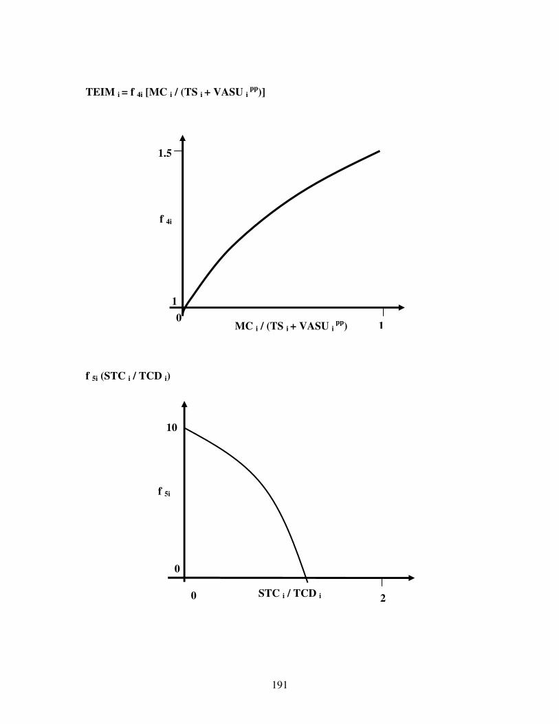
191

TEIM i = f 4i [MC i / (TS i + VASU i pp)] f 5i (STC i / TCD i)

f 4i

1 0

1.5

MC i / (TS i + VASU i pp)

1

f 5i

2

0

10

STC i / TCD i 0

192

PFVAS i m = f 5i (PVAS i m / NPVAS i m)

NLTDA i = f 7i (WNTD i)

f 6i

2 3 0

1

PVAS i m / NPVAS i m

1

f 7i

1

1

5

WNTD i 0

193

APPENDIX B: MODEL LISTINGS

EQUATIONS OF THE REGIONAL TELECOM SYSTEM TELEPHONE DEPLOYMENT EQUATIONS:

Avg_Connection_Rate[Urban](t) = Avg_Connection_Rate[Urban](t - dt) + (Avg_Con_Capac_Change[Urban]) * dt INIT Avg_Connection_Rate[Urban] = 0 Avg_Connection_Rate[Rural](t) = Avg_Connection_Rate[Rural](t - dt) + (Avg_Con_Capac_Change[Rural]) * dt INIT Avg_Connection_Rate[Rural] = 0 INFLOWS:

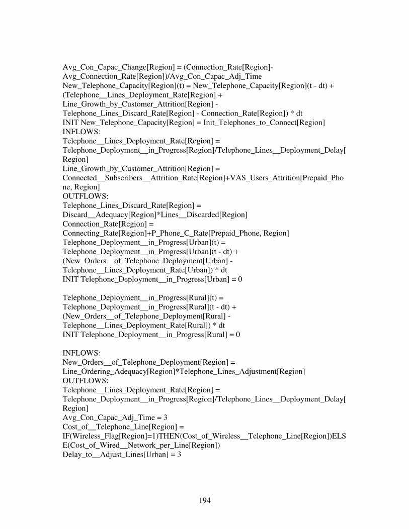
194

Avg_Con_Capac_Change[Region] = (Connection_Rate[Region]-Avg_Connection_Rate[Region])/Avg_Con_Capac_Adj_Time New_Telephone_Capacity[Region](t) = New_Telephone_Capacity[Region](t - dt) + (Telephone__Lines_Deployment_Rate[Region] + Line_Growth_by_Customer_Attrition[Region] - Telephone_Lines_Discard_Rate[Region] - Connection_Rate[Region]) * dt INIT New_Telephone_Capacity[Region] = Init_Telephones_to_Connect[Region] INFLOWS: Telephone__Lines_Deployment_Rate[Region] = Telephone_Deployment__in_Progress[Region]/Telephone_Lines__Deployment_Delay[Region] Line_Growth_by_Customer_Attrition[Region] = Connected__Subscribers__Attrition_Rate[Region]+VAS_Users_Attrition[Prepaid_Phone, Region] OUTFLOWS: Telephone_Lines_Discard_Rate[Region] = Discard__Adequacy[Region]*Lines__Discarded[Region] Connection_Rate[Region] = Connecting_Rate[Region]+P_Phone_C_Rate[Prepaid_Phone, Region] Telephone_Deployment__in_Progress[Urban](t) = Telephone_Deployment__in_Progress[Urban](t - dt) + (New_Orders__of_Telephone_Deployment[Urban] - Telephone__Lines_Deployment_Rate[Urban]) * dt INIT Telephone_Deployment__in_Progress[Urban] = 0 Telephone_Deployment__in_Progress[Rural](t) = Telephone_Deployment__in_Progress[Rural](t - dt) + (New_Orders__of_Telephone_Deployment[Rural] - Telephone__Lines_Deployment_Rate[Rural]) * dt INIT Telephone_Deployment__in_Progress[Rural] = 0 INFLOWS: New_Orders__of_Telephone_Deployment[Region] = Line_Ordering_Adequacy[Region]*Telephone_Lines_Adjustment[Region] OUTFLOWS: Telephone__Lines_Deployment_Rate[Region] = Telephone_Deployment__in_Progress[Region]/Telephone_Lines__Deployment_Delay[Region] Avg_Con_Capac_Adj_Time = 3 Cost_of__Telephone_Line[Region] = IF(Wireless_Flag[Region]=1)THEN(Cost_of_Wireless__Telephone_Line[Region])ELSE(Cost_of_Wired__Network_per_Line[Region]) Delay_to__Adjust_Lines[Urban] = 3

195

Delay_to__Adjust_Lines[Rural] = 3 Demanded_Telephone__Lines[Region] = Waiting_List[Region]+PPWaiting_Lines[Region] Desired_Telephone_Capacity[Region] = Supplied__Telephone_Lines[Region]-Afforded__Expected_Adequacy[Region]*(Supplied__Telephone_Lines[Region]-Demanded_Telephone__Lines[Region]) Init_Telephones_to_Connect[Urban] = 10000 Init_Telephones_to_Connect[Rural] = 100 Lines__Discarded[Region] = Telephone_Lines_Adjustment[Region]*Lines_Adjustment_Adequacy[Region] PPWaiting_Lines[Region] = Prepaid_Phone_Waiting_List[Region]*Lines_per_VAS_Users Supplied__Telephone_Lines[Region] = Potential_Region_Investment[Region]/Cost_of__Telephone_Line[Region] Telephone_Lines_Adjustment[Region] = Avg_Connection_Rate[Region]+(Desired_Telephone_Capacity[Region]-New_Telephone_Capacity[Region]-Telephone_Deployment__in_Progress[Region])/Delay_to__Adjust_Lines[Region] Telephone_Lines__Deployment_Delay[Region] = IF(Wireless_Flag[Region]=1)THEN(Wireless_Line_Deployment_Time[Region])ELSE(Time_to_Deploy_Telephone_Line[Region]) Wireless_Flag[Region] = 0 Wireless_Line_Deployment_Time[Urban] = 6 Wireless_Line_Deployment_Time[Rural] = 8 Afforded__Expected_Adequacy[Region] = GRAPH(Supplied__Telephone_Lines[Region]/(Demanded_Telephone__Lines[Region]+0.0001)) (1.00, 0.00), (1.01, 0.38), (1.02, 0.68), (1.03, 0.825), (1.04, 0.91), (1.05, 0.97), (1.06, 0.995), (1.07, 1.00), (1.08, 1.00), (1.09, 1.00), (1.10, 1.00) Discard__Adequacy[Region] = GRAPH(New_Telephone_Capacity[Region]/(Lines__Discarded[Region]+1)) (0.00, 0.00), (1.00, 0.335), (2.00, 0.535), (3.00, 0.705), (4.00, 0.82), (5.00, 0.895), (6.00, 0.94), (7.00, 0.975), (8.00, 0.99), (9.00, 1.00), (10.0, 1.00) Lines_Adjustment_Adequacy[Region] = GRAPH(Telephone_Lines_Adjustment[Region]) (-1.00, -1.00), (-0.9, -0.7), (-0.8, -0.45), (-0.7, -0.295), (-0.6, -0.19), (-0.5, -0.115), (-0.4, -0.065), (-0.3, -0.025), (-0.2, -0.01), (-0.1, -0.005), (-1.39e-016, 0.00) Line_Ordering_Adequacy[Region] = GRAPH(Telephone_Lines_Adjustment[Region]) (0.00, 0.00), (0.1, 0.275), (0.2, 0.5), (0.3, 0.66), (0.4, 0.78), (0.5, 0.865), (0.6, 0.92), (0.7, 0.955), (0.8, 0.975), (0.9, 0.99), (1, 1.00)

196

FINANCIAL RESOURCES EQUATIONS:

197

Telecom_Cash__Balance(t) = Telecom_Cash__Balance(t - dt) + (Telecom_Income - Telecom__Expenses) * dt INIT Telecom_Cash__Balance = Initial_Cash_Balance INFLOWS: Telecom_Income = Total_Telephone_Serv_Income+Activation_Income[Urban]+Activation_Income[Rural]+Net_Settlement+Total_VAS_Income OUTFLOWS: Telecom__Expenses = Actual_T_Line_Investment_per__Month[Urban]+Actual_T_Line_Investment_per__Month[Rural]+Operating_costs[Urban]+Operating_costs[Rural]+Total_VAS__Investment+License_Expense Activation_Fee[Urban] = 76 Activation_Fee[Rural] = 22 Activation_Income[Region] = Activation_Fee[Region]*(Connecting_Rate[Region]+P_Phone_C_Rate[Prepaid_Phone, Region]*Lines_per_VAS_Users) Actual_T_Line_Investment_per__Month[Region] = New_Orders__of_Telephone_Deployment[Region]*Cost_of__Telephone_Line[Region] Capital__Costs[Region] = Telephone__Capital_Costs[Region]+VAS_Capital_Costs[Region] CCard_Infra_per_User = 1 CCard__Infra[Region] = (VAS_Users[Virtual_Telephony,Region]+VAS_Users[Payphone,Region]+VAS_Users[Prepaid_Phone,Region])*CCard_Infra_per_User Fraction_of_Cap_Costs_as_part_of_Operating_Costs = 0.3 Free_Service__Minutes[URLOCAL] = 100 Free_Service__Minutes[RULOCAL] = 100 Free_Service__Minutes[INTERURB] = 0.0001 Free_Service__Minutes[INTERRUR] = 0.0001 Free_Service__Minutes[LDURB] = 0.0001 Free_Service__Minutes[LDRUR] = 0.0001 Imbalance_Internat_Traffic_per_Subscriber[Urban] = Incoming_International_Traffic[Urban]-Service_Time_per_Line[INTERURB] Imbalance_Internat_Traffic_per_Subscriber[Rural] = IF(Incoming_International_Traffic[Rural]-Service_Time_per_Line[INTERRUR] > 0 ) THEN (Incoming_International_Traffic[Rural]-Service_Time_per_Line[INTERRUR]) ELSE (0) Initial_Cash_Balance = 0 Inv_Fract = 1

198

License_Expense = License__Cost/License__Duration/Months_per_Year License__Cost = 0 License__Duration = 15 Maibox_Infra[Region] = VAS_Users[Virtual_Telephony,Region]*Mailbox_Infra_per_User Mailbox_Infra_per_User = 1 Monthly_Fraction_Operating_Costs = 1/12 Net_Settlement = (Total_Phone_Lines[Urban]*Imbalance_Internat_Traffic_per_Subscriber[Urban]*Settlement_Rate)+(Total_Phone_Lines[Rural]*Imbalance_Internat_Traffic_per_Subscriber[Rural]*Settlement_Rate) New_CCard_Infrastructure[Region] = (VAS_Adoption[Virtual_Telephony,Region]+VAS_Adoption[Payphone,Region]+P_Phone_C_Rate[Prepaid_Phone,Region])*CCard_Infra_per_User New_Mailbox_Infrastructure[Region] = VAS_Adoption[Virtual_Telephony,Region]*Mailbox_Infra_per_User New_Payphone_Infrastructure[Region] = New_Orders__of_Payphone_Deployment[Payphones, Region] Operating_costs[Region] = Capital__Costs[Region]*Fraction_of_Cap_Costs_as_part_of_Operating_Costs*Monthly_Fraction_Operating_Costs Payphone_Infrastructure[Region] = Payphone__Installed[Payphones, Region]+Payphone_Deployment__in_Progress[Payphones, Region] Payphone_Total_Investment = Potential_Total__Investment*VAS__Investment_Fraction Potential_Region_Investment[Urban] = Potential_Total__Investment*Urban_Inv_Fr+0*Rural_Investment_Fraction Potential_Region_Investment[Rural] = Potential_Total__Investment*Rural_Investment_Fraction+0*Urban_Inv_Fr Potential_Total__Investment = Telecom_Cash__Balance*Inv_Fract*Investment__Adequacy Rural_Investment_Fraction = Universal_Service__Obligation Service_Customers[URLOCAL] = Connected__Subscribers[Urban] Service_Customers[RULOCAL] = Connected__Subscribers[Rural] Service_Customers[INTERURB] = Connected__Subscribers[Urban] Service_Customers[INTERRUR] = Connected__Subscribers[Rural] Service_Customers[LDURB] = Connected__Subscribers[Urban] Service_Customers[LDRUR] = Connected__Subscribers[Rural] Settlement_Rate = Price_of_Traffic_per_Service[INTERURB]/2 Telephone_Service__Income[URLOCAL] = ((Price_of_Traffic_per_Service[URLOCAL]*(Service_Time_per_Line[URLOCAL]-Free_Service__Minutes[URLOCAL])*Local_Time_Adequacy[URLOCAL])+M_Rental_Fee[Urban])*Service_Customers[URLOCAL]

199

Telephone_Service__Income[RULOCAL] = ((Price_of_Traffic_per_Service[RULOCAL]*(Service_Time_per_Line[RULOCAL]-Free_Service__Minutes[RULOCAL])*Local_Time_Adequacy[RULOCAL])+M_Rental_Fee[Rural])*Service_Customers[RULOCAL] Telephone_Service__Income[INTERURB] = (Price_of_Traffic_per_Service[INTERURB]*Service_Customers[INTERURB]*Service_Time_per_Line[INTERURB])+0*M_Rental_Fee[Urban]*Free_Service__Minutes[INTERURB]*Local_Time_Adequacy[INTERURB] Telephone_Service__Income[INTERRUR] = (Price_of_Traffic_per_Service[INTERRUR]*Service_Customers[INTERRUR]*Service_Time_per_Line[INTERRUR])+0*M_Rental_Fee[Urban]*Free_Service__Minutes[INTERRUR]*Local_Time_Adequacy[INTERRUR] Telephone_Service__Income[LDURB] = Service_Time_per_Line[LDURB]*Price_of_Traffic_per_Service[LDURB]*Service_Customers[LDURB]+0*M_Rental_Fee[Urban]*Free_Service__Minutes[LDURB]*Local_Time_Adequacy[LDURB] Telephone_Service__Income[LDRUR] = Service_Time_per_Line[LDRUR]*Price_of_Traffic_per_Service[LDRUR]*Service_Customers[LDRUR]+0*M_Rental_Fee[Rural]*Free_Service__Minutes[LDRUR]*Local_Time_Adequacy[LDRUR] Telephone__Capital_Costs[Region] = Cost_of__Telephone_Line[Region]*Total_Telephone_Lines[Region] Total_Telephone_Lines[Region] = Connected__Subscribers[Region]+New_Telephone_Capacity[Region]+Telephone_Deployment__in_Progress[Region]+Prepaid_Tel_Lines[Region] Total_Telephone_Serv_Income = Telephone_Service__Income[URLOCAL]+Telephone_Service__Income[RULOCAL]+Telephone_Service__Income[INTERURB]+Telephone_Service__Income[INTERRUR]+Telephone_Service__Income[LDURB]+Telephone_Service__Income[LDRUR] Total_VAS_Income = VAS__Income[Virtual_Telephony,Urban]+VAS__Income[Virtual_Telephony,Rural]+VAS__Income[Payphone,Urban]+VAS__Income[Payphone,Rural]+VAS__Income[Prepaid_Phone,Urban]+VAS__Income[Prepaid_Phone,Rural] Total_VAS__Investment = VAS_Investment_per_Month[Urban]+VAS_Investment_per_Month[Rural] Urban_Inv_Fr = 1-Rural_Investment_Fraction-VAS__Investment_Fraction VAS_Capital_Costs[Region] = Maibox_Infra[Region]*Cost_of_each_Mail_Box+Payphone_Infrastructure[Region]*Cost_of_each_Payphone[Region]+CCard__Infra[Region]*Cost_Calling_Card_Number VAS_Investment_per_Month[Region] = New_Mailbox_Infrastructure[Region]*Cost_of_each_Mail_Box+New_CCard_Infrastructure[Region]*Cost_Calling_Card_Number+New_Payphone_Infrastructure[Region]*Cost_of_each_Payphone[Region]

200

VAS__Income[VAS,Region] = VAS_Users[VAS,Region]*VAS_Price[VAS,Region] VAS__Investment_Fraction = VAS_Investment_Policy Investment__Adequacy = GRAPH(Telecom_Cash__Balance) (0.00, 0.00), (100, 0.00), (200, 0.01), (300, 0.04), (400, 0.07), (500, 0.11), (600, 0.165), (700, 0.25), (800, 0.385), (900, 0.595), (1000, 1.00) Local_Time_Adequacy[Service] = GRAPH(Service_Time_per_Line[Service]/Free_Service__Minutes[Service]) (0.99, 0.00), (0.991, 0.475), (0.992, 0.76), (0.993, 0.94), (0.994, 1.00), (0.995, 1.00), (0.996, 1.00), (0.997, 1.00), (0.998, 1.00), (0.999, 1.00), (1.00, 1.00)

201

TELEPHONE DEMAND EQUATIONS:

Connected__Subscribers[Region](t) = Connected__Subscribers[Region](t - dt) + (Connecting_Rate[Region] - Connected__Subscribers__Attrition_Rate[Region]) * dt

202

INIT Connected__Subscribers[Region] = Con_Subscribers_Init[Region] INFLOWS: Connecting_Rate[Region] = Connecting_Rate_Indicated[Region]*Waiting_List_Restriction[Region] OUTFLOWS: Connected__Subscribers__Attrition_Rate[Region] = Attrition_Rate_Indicated[Region]*Attrition_Rate_Adequacy[Region] Effect_of_Attractiveness_on_Demand[Region](t) = Effect_of_Attractiveness_on_Demand[Region](t - dt) + (Attractiveness__Growth[Region]) * dt INIT Effect_of_Attractiveness_on_Demand[Region] = Effect_Attract_on_Demand_Indicated[Region] INFLOWS: Attractiveness__Growth[Region] = (Effect_Attract_on_Demand_Indicated[Region]-Effect_of_Attractiveness_on_Demand[Region])/Time_to_Recognize_Attractiveness Population[Region](t) = Population[Region](t - dt) + (Population_Growth[Region]) * dt INIT Population[Region] = Init_Region_Population[Region] INFLOWS: Population_Growth[Region] = Population[Region]*Population_Rate_of_Growth_Month[Region] Population_of_Telephone_Subscribers[Region](t) = Population_of_Telephone_Subscribers[Region](t - dt) + (Pop_Tel_Subsc_Growth[Region]) * dt INIT Population_of_Telephone_Subscribers[Region] = Init_Pop_Tel_Subs[Region] INFLOWS: Pop_Tel_Subsc_Growth[Region] = Population_of_Telephone_Subscribers[Region]*Population_Rate_of_Growth_Month[Region] Potential__Customers[Urban](t) = Potential__Customers[Urban](t - dt) + (New_Potential__Customer_Rate[Urban] - Rate_of_New_Customers[Urban]) * dt INIT Potential__Customers[Urban] = 0 Potential__Customers[Rural](t) = Potential__Customers[Rural](t - dt) + (New_Potential__Customer_Rate[Rural] - Rate_of_New_Customers[Rural]) * dt INIT Potential__Customers[Rural] = 0 INFLOWS: New_Potential__Customer_Rate[Region] = New_Potential_Customers__Rate_Indicated[Region]*New_Pot_Cus_Rate_Adequacy[Region] OUTFLOWS: Rate_of_New_Customers[Region] = Potential__Customers[Region]/Delay_to_Accept_Activation_Fee

203

Pot_Customers_without_Interest_on_Tel_Services[Region](t) = Pot_Customers_without_Interest_on_Tel_Services[Region](t - dt) + (PCWIOTS_Growth[Region] - New_Potential__Customer_Rate[Region] - Prep_Phone_Lines_Growth[Region]) * dt INIT Pot_Customers_without_Interest_on_Tel_Services[Region] = Init_Pot_Cust__WIOTS[Region] INFLOWS: PCWIOTS_Growth[Region] = Pop_Tel_Subsc_Growth[Region]+Connected__Subscribers__Attrition_Rate[Region]+Prep_Phone__Demand_Reduction[Region] OUTFLOWS: New_Potential__Customer_Rate[Region] = New_Potential_Customers__Rate_Indicated[Region]*New_Pot_Cus_Rate_Adequacy[Region] Prep_Phone_Lines_Growth[Region] = Prep_Phone_Demand_Growth[Region]*Lines_per_VAS_Users Prepaid_Phone_Demand[Region](t) = Prepaid_Phone_Demand[Region](t - dt) + (Prep_Phone_Lines_Growth[Region] - Prep_Phone__Demand_Reduction[Region]) * dt INIT Prepaid_Phone_Demand[Region] = 0 INFLOWS: Prep_Phone_Lines_Growth[Region] = Prep_Phone_Demand_Growth[Region]*Lines_per_VAS_Users OUTFLOWS: Prep_Phone__Demand_Reduction[Region] = VAS_Users_Attrition[Prepaid_Phone, Region] Waiting_List[Region](t) = Waiting_List[Region](t - dt) + (Rate_of_New_Customers[Region] - Connecting_Rate[Region]) * dt INIT Waiting_List[Region] = Waiting_List_Init_[Region] INFLOWS: Rate_of_New_Customers[Region] = Potential__Customers[Region]/Delay_to_Accept_Activation_Fee OUTFLOWS: Connecting_Rate[Region] = Connecting_Rate_Indicated[Region]*Waiting_List_Restriction[Region] Actual_Demand[Region] = Connected__Subscribers[Region]+Potential__Customers[Region]+Waiting_List[Region] Attrition_Rate_Indicated[Region] = Demand_Adjustment[Region]*Attrition_Adequacy[Region] Connecting_Rate_Indicated[Region] = New_Telephone_Capacity[Region]*Fraction_of_Tel_Capacity_Con_per_Month*Conventional_Prepaid_Fr[Region] Con_Subscribers_Init[Urban] = Total_Con_Subs_Initial*(1-Percent_Rural_Lines)

204

Con_Subscribers_Init[Rural] = Total_Con_Subs_Initial*Percent_Rural_Lines Delay_to_Accept_Activation_Fee = 3 Demand_Adjustment[Region] = (Indicated__Demand[Region]-Actual_Demand[Region])/Time_to_Adjust_Demand[Region] Demand_Fractrion[Region] = Effect_of_Attractiveness_on_Demand[Region]*Effect_of__Price_on_Demand[Region] Effect_Attract_on_Demand_Indicated[Region] = Network_Externality_Impact[Region] Effect_of__Price_on_Demand[Region] = Monthly__Rental_Fraction[Region] Fraction_of_Tel_Capacity_Con_per_Month = 0.25 Fr_of_Exp_Telecom[Urban] = 0.015 Fr_of_Exp_Telecom[Rural] = 0.015 Income_per_Capita[Urban] = 1708 Income_per_Capita[Rural] = 310 Indicated__Demand[Region] = Population_of_Telephone_Subscribers[Region]*Demand_Fractrion[Region] Initial_Total_Population = 23000000 Init_Pop_Tel_Subs[Region] = Init_Region_Population[Region]*Number_of_Lines_per_People[Region] Init_Pot_Cust__WIOTS[Region] = Init_Pop_Tel_Subs[Region]-Waiting_List_Init_[Region]-Con_Subscribers_Init[Region] Init_Region_Population[Urban] = Initial_Total_Population*(1-Perc_Rural_Pop) Init_Region_Population[Rural] = Initial_Total_Population*Perc_Rural_Pop ITU_Waitiing_List = 86022 Lines_per_VAS_Users = 1 Minimum_Subs_Discarded = 1 Min_Con_Rate = 1 Min_New_Pot_Cust_Rate = 1 Mionthly_Income_per_Capita[Region] = Income_per_Capita[Region]*Year_Month_Relation Monthly_Income_per_Subscriber[Region] = Mionthly_Income_per_Capita[Region]/Number_of_Lines_per_People[Region] Monthly_Rental_Discrepancy[Region] = M_Rental_Fee[Region]/Normal_Monthly_Rental[Region] Monthly__Rental_Fraction[Region] = Monthly_Rental_Discrepancy[Region] Months_per_Year = 12 Network_Externality_Impact[Region] = Region_Externality_Impact[Region] New_Potential_Customers__Rate_Indicated[Region] = Demand_Adjustment[Region]*New_Subscribers_Adequacy[Region] Number_of_Lines_per_People[Region] = Num_of_Lines_per_House[Region]/Num_of_People_per_House[Region] Num_of_Lines_per_House[Urban] = 1 Num_of_Lines_per_House[Rural] = 1 Num_of_People_per_House[Region] = 4

205

Percent_Rural_Lines = 0.1 Perc_Rural_Pop = 0.4 Population_Rate_of_Growth_Month[Region] = ((1+Population_Rate_of_Growth_Year[Region])^(1/Months_per_Year))-1 Population_Rate_of_Growth_Year[Urban] = 0.023 Population_Rate_of_Growth_Year[Rural] = 0.002 Prepaid_Tel_Lines[Region] = VAS_Users[Prepaid_Phone, Region]*Lines_per_VAS_Users Prep_Phone_Demand_Growth[Region] = VAS_Increase[Prepaid_Phone, Region]*New_Pot_Cus_Rate_Adequacy[Region] Ref_Tel_Exp_per_Line[Region] = Fr_of_Exp_Telecom[Region]*Monthly_Income_per_Subscriber[Region]*Telecom_Expenditure_Incr_Size_of_the_Network[Region] Regional_Fraction_W_List[Urban] = 0.9 Regional_Fraction_W_List[Rural] = 0.1 Region_Externality_Impact[Region] = Region_Telephone_Density[Urban]*Urban_Weight_on_Externality[Region]+Region_Telephone_Density[Rural]*Rural_Weight_on_Externality[Region] Region_Telephone_Density[Region] = (Connected__Subscribers[Region]+VTelephony_Lines[Region]+Prepaid_Tel_Lines[Region])/Population_of_Telephone_Subscribers[Region] Rural_Weight_on_Externality[Urban] = 0.1 Rural_Weight_on_Externality[Rural] = 0.5 Susbcriber__Expenditure_on_Telecommunications_[Region] = Ref_Tel_Exp_per_Line[Region]*Telecom_Expenditure_Increase_from_Mobility[Region] Telecom_Expenditure_Incr_Size_of_the_Network[Region] = Region_Externality_Impact[Region] Time_to_Adjust_Demand[Region] = 60 Time_to_Recognize_Attractiveness = 6 Total_Con_Subs_Initial = 598287 Urban_Weight_on_Externality[Urban] = 0.9 Urban_Weight_on_Externality[Rural] = 0.5 VTelephony_Lines[Region] = VAS_Users[Virtual_Telephony, Region]*Lines_per_VAS_Users Waiting_List_Initial = ITU_Waitiing_List*Waiting_List_Unreported_Factor Waiting_List_Init_[Urban] = Waiting_List_Initial*Regional_Fraction_W_List[Urban] Waiting_List_Init_[Rural] = Waiting_List_Initial*Regional_Fraction_W_List[Rural] Waiting_List_Unreported_Factor = 4 Year_Month_Relation = 1/12 Attrition_Adequacy[Region] = GRAPH(Demand_Adjustment[Region]) (-1.00, -1.00), (-0.9, -0.99), (-0.8, -0.97), (-0.7, -0.915), (-0.6, -0.775), (-0.5, -0.505), (-0.4, -0.255), (-0.3, -0.115), (-0.2, -0.045), (-0.1, -0.01), (-1.39e-016, 0.00)

206

Attrition_Rate_Adequacy[Region] = GRAPH(Connected__Subscribers[Region]/(Attrition_Rate_Indicated[Region]+Minimum_Subs_Discarded)) (0.00, 0.00), (0.5, 0.01), (1.00, 0.055), (1.50, 0.135), (2.00, 0.27), (2.50, 0.505), (3.00, 0.745), (3.50, 0.895), (4.00, 0.985), (4.50, 1.00), (5.00, 1.00) Monthly__Rental_Fraction[Region] = Monthly_Rental_Discrepancy[Region] New_Pot_Cus_Rate_Adequacy[Region] = GRAPH(Pot_Customers_without_Interest_on_Tel_Services[Region]/(New_Potential_Customers__Rate_Indicated[Region]+VAS_Increase[Prepaid_Phone, Region]*Lines_per_VAS_Users+Min_New_Pot_Cust_Rate)) (0.00, 0.00), (0.4, 0.025), (0.8, 0.085), (1.20, 0.185), (1.60, 0.33), (2.00, 0.5), (2.40, 0.715), (2.80, 0.84), (3.20, 0.92), (3.60, 0.98), (4.00, 1.00) New_Subscribers_Adequacy[Region] = GRAPH(Demand_Adjustment[Region]) (0.00, 0.00), (0.1, 0.31), (0.2, 0.515), (0.3, 0.66), (0.4, 0.765), (0.5, 0.85), (0.6, 0.915), (0.7, 0.96), (0.8, 0.985), (0.9, 0.99), (1, 1.00) Region_Externality_Impact[Region] = Region_Telephone_Density[Urban]*Urban_Weight_on_Externality[Region]+Region_Telephone_Density[Rural]*Rural_Weight_on_Externality[Region] Telecom_Expenditure_Increase_from_Mobility[Region] = GRAPH(Fraction_of_Mobile_Subscribers[Region]) (0.00, 1.00), (0.1, 1.03), (0.2, 1.08), (0.3, 1.17), (0.4, 1.29), (0.5, 1.38), (0.6, 1.45), (0.7, 1.48), (0.8, 1.50), (0.9, 1.50), (1, 1.50) Telecom_Expenditure_Incr_Size_of_the_Network[Region] = Region_Externality_Impact[Region] Waiting_List_Restriction[Region] = GRAPH(Waiting_List[Region]/(Connecting_Rate_Indicated[Region]+Min_Con_Rate)) (0.00, 0.00), (0.5, 0.035), (1.00, 0.07), (1.50, 0.105), (2.00, 0.145), (2.50, 0.215), (3.00, 0.37), (3.50, 0.65), (4.00, 0.795), (4.50, 0.915), (5.00, 1.00)

207

TELEPHONE TRAFFIC EQUATIONS:

Service_Time_per_Line[Service](t) = Service_Time_per_Line[Service](t - dt) + (Service_Time_Adjustment_Rate[Service]) * dt INIT Service_Time_per_Line[Service] = Referential_Service_Time_per_Line[Service] INFLOWS:

208

Service_Time_Adjustment_Rate[Service] = (Referential_Service_Time_per_Line[Service]-Service_Time_per_Line[Service])/Service_Time_Adj_Period[Service] Expenditure_on_Traffic_per_line[Region] = Normal_Expenditure_on_Traffic[Region]*Telecom_Expenditure_Incr_Size_of_the_Network[Region]*Telecom_Expenditure_Increase_from_Mobility[Region] Exp_on_Traffic_as_Fraction_of_Income[Urban] = 0.010 Exp_on_Traffic_as_Fraction_of_Income[Rural] = 0.006 Fraction_of__Expenditure_per__Service[URLOCAL] = 0.3 Fraction_of__Expenditure_per__Service[RULOCAL] = 0 Fraction_of__Expenditure_per__Service[INTERURB] = 0.5 Fraction_of__Expenditure_per__Service[INTERRUR] = 0.2 Fraction_of__Expenditure_per__Service[LDURB] = 0.2 Fraction_of__Expenditure_per__Service[LDRUR] = 0.8 Free_Local_Minutes_Used[Urban] = 100 Free_Local_Minutes_Used[Rural] = 50 Incoming_International_Traffic[Urban] = Service_Time_per_Line[INTERURB]*Incoming_Outgoing_International_Traffic_Ratio Incoming_International_Traffic[Rural] = Service_Time_per_Line[INTERRUR]*Incoming_Outgoing_International_Traffic_Ratio Incoming_Outgoing_International_Traffic_Ratio = 3 Indicated_Traffic_Expenditure_per_Service[URLOCAL] = Expenditure_on_Traffic_per_line[Urban]*Fraction_of__Expenditure_per__Service[URLOCAL] Indicated_Traffic_Expenditure_per_Service[RULOCAL] = Expenditure_on_Traffic_per_line[Rural]*Fraction_of__Expenditure_per__Service[RULOCAL] Indicated_Traffic_Expenditure_per_Service[INTERURB] = Expenditure_on_Traffic_per_line[Urban]*Fraction_of__Expenditure_per__Service[INTERURB] Indicated_Traffic_Expenditure_per_Service[INTERRUR] = Expenditure_on_Traffic_per_line[Rural]*Fraction_of__Expenditure_per__Service[INTERRUR] Indicated_Traffic_Expenditure_per_Service[LDURB] = Expenditure_on_Traffic_per_line[Urban]*Fraction_of__Expenditure_per__Service[LDURB] Indicated_Traffic_Expenditure_per_Service[LDRUR] = Expenditure_on_Traffic_per_line[Rural]*Fraction_of__Expenditure_per__Service[LDRUR]

209

Normal_Expenditure_on_Traffic[Region] = Exp_on_Traffic_as_Fraction_of_Income[Region]*Monthly_Income_per_Subscriber[Region] Normal_Monthly_Rental[Region] = (W_t_Pay_Telephone_Service[Region]-Expenditure_on_Traffic_per_line[Region])*Normal_Monthly_Rental_Adequacy[Region] Price_of_Traffic_per_Service[URLOCAL] = 0.014 Price_of_Traffic_per_Service[RULOCAL] = 0.002 Price_of_Traffic_per_Service[INTERURB] = 1 Price_of_Traffic_per_Service[INTERRUR] = 1 Price_of_Traffic_per_Service[LDURB] = 0.042 Price_of_Traffic_per_Service[LDRUR] = 0.006 Referential_Service_Time_per_Line[URLOCAL] = Referential_Service_Time_per_Line_Indicated[URLOCAL]+Free_Local_Minutes_Used[Urban] Referential_Service_Time_per_Line[RULOCAL] = Referential_Service_Time_per_Line_Indicated[RULOCAL]+Free_Local_Minutes_Used[Rural] Referential_Service_Time_per_Line[INTERURB] = Referential_Service_Time_per_Line_Indicated[INTERURB]+0*Free_Local_Minutes_Used[Urban] Referential_Service_Time_per_Line[INTERRUR] = Referential_Service_Time_per_Line_Indicated[INTERRUR]+0*Free_Local_Minutes_Used[Rural] Referential_Service_Time_per_Line[LDURB] = Referential_Service_Time_per_Line_Indicated[LDURB]+0*Free_Local_Minutes_Used[Urban] Referential_Service_Time_per_Line[LDRUR] = Referential_Service_Time_per_Line_Indicated[LDRUR]+0*Free_Local_Minutes_Used[Rural] Referential_Service_Time_per_Line_Indicated[URLOCAL] = (Indicated_Traffic_Expenditure_per_Service[URLOCAL]/Price_of_Traffic_per_Service[URLOCAL]) Referential_Service_Time_per_Line_Indicated[RULOCAL] = (Indicated_Traffic_Expenditure_per_Service[RULOCAL]/Price_of_Traffic_per_Service[RULOCAL]) Referential_Service_Time_per_Line_Indicated[INTERURB] = Indicated_Traffic_Expenditure_per_Service[INTERURB]/Price_of_Traffic_per_Service[INTERURB] Referential_Service_Time_per_Line_Indicated[INTERRUR] = Indicated_Traffic_Expenditure_per_Service[INTERRUR]/Price_of_Traffic_per_Service[INTERRUR]

210

Referential_Service_Time_per_Line_Indicated[LDURB] = Indicated_Traffic_Expenditure_per_Service[LDURB]/Price_of_Traffic_per_Service[LDURB] Referential_Service_Time_per_Line_Indicated[LDRUR] = Indicated_Traffic_Expenditure_per_Service[LDRUR]/Price_of_Traffic_per_Service[LDRUR] Service_Time_Adj_Period[Service] = 12 W_t_Pay_Telephone_Service[Region] = Susbcriber__Expenditure_on_Telecommunications_[Region] Normal_Monthly_Rental_Adequacy[Region] = GRAPH(W_t_Pay_Telephone_Service[Region]/Expenditure_on_Traffic_per_line[Region]) (1.00, 0.00), (1.00, 0.295), (1.01, 0.555), (1.01, 0.765), (1.02, 0.87), (1.02, 0.94), (1.03, 0.96), (1.03, 0.975), (1.04, 0.99), (1.04, 0.995), (1.05, 1.00)

211

VALUE ADDED SERVICE DEMAND EQUATIONS:

Potential_VAS_Users[Virtual_Telephony,Urban](t) = Potential_VAS_Users[Virtual_Telephony,Urban](t - dt) +

212

(Potential_VAS_Growth[Virtual_Telephony,Urban] + Potential_VAS_Growth_from_Attrition[Virtual_Telephony,Urban] - VAS_Adoption[Virtual_Telephony,Urban] - Potential_VAS__Reduction[Virtual_Telephony,Urban] - Prepaid_Phone_New_Customers[Virtual_Telephony,Urban]) * dt INIT Potential_VAS_Users[Virtual_Telephony,Urban] = (Waiting_List[Urban]/Lines_per_VAS_Users+Prepaid_Phone_Waiting_List[Urban])*VAS_Offered[Virtual_Telephony,Urban] Potential_VAS_Users[Virtual_Telephony,Rural](t) = Potential_VAS_Users[Virtual_Telephony,Rural](t - dt) + (Potential_VAS_Growth[Virtual_Telephony,Rural] + Potential_VAS_Growth_from_Attrition[Virtual_Telephony,Rural] - VAS_Adoption[Virtual_Telephony,Rural] - Potential_VAS__Reduction[Virtual_Telephony,Rural] - Prepaid_Phone_New_Customers[Virtual_Telephony,Rural]) * dt INIT Potential_VAS_Users[Virtual_Telephony,Rural] = (Waiting_List[Rural]/Lines_per_VAS_Users+Prepaid_Phone_Waiting_List[Rural])*VAS_Offered[Virtual_Telephony,Rural] Potential_VAS_Users[Payphone,Urban](t) = Potential_VAS_Users[Payphone,Urban](t - dt) + (Potential_VAS_Growth[Payphone,Urban] + Potential_VAS_Growth_from_Attrition[Payphone,Urban] - VAS_Adoption[Payphone,Urban] - Potential_VAS__Reduction[Payphone,Urban] - Prepaid_Phone_New_Customers[Payphone,Urban]) * dt INIT Potential_VAS_Users[Payphone,Urban] = Population[Urban]*payphone_users_per_people[Urban] Potential_VAS_Users[Payphone,Rural](t) = Potential_VAS_Users[Payphone,Rural](t - dt) + (Potential_VAS_Growth[Payphone,Rural] + Potential_VAS_Growth_from_Attrition[Payphone,Rural] - VAS_Adoption[Payphone,Rural] - Potential_VAS__Reduction[Payphone,Rural] - Prepaid_Phone_New_Customers[Payphone,Rural]) * dt INIT Potential_VAS_Users[Payphone,Rural] = Population[Rural]*payphone_users_per_people[Rural] Potential_VAS_Users[Prepaid_Phone,Urban](t) = Potential_VAS_Users[Prepaid_Phone,Urban](t - dt) + (Potential_VAS_Growth[Prepaid_Phone,Urban] + Potential_VAS_Growth_from_Attrition[Prepaid_Phone,Urban] - VAS_Adoption[Prepaid_Phone,Urban] - Potential_VAS__Reduction[Prepaid_Phone,Urban] - Prepaid_Phone_New_Customers[Prepaid_Phone,Urban]) * dt

213

INIT Potential_VAS_Users[Prepaid_Phone,Urban] = Pot_Customers_without_Interest_on_Tel_Services[Urban]*VAS_Offered[Prepaid_Phone,Urban] Potential_VAS_Users[Prepaid_Phone,Rural](t) = Potential_VAS_Users[Prepaid_Phone,Rural](t - dt) + (Potential_VAS_Growth[Prepaid_Phone,Rural] + Potential_VAS_Growth_from_Attrition[Prepaid_Phone,Rural] - VAS_Adoption[Prepaid_Phone,Rural] - Potential_VAS__Reduction[Prepaid_Phone,Rural] - Prepaid_Phone_New_Customers[Prepaid_Phone,Rural]) * dt INIT Potential_VAS_Users[Prepaid_Phone,Rural] = Pot_Customers_without_Interest_on_Tel_Services[Rural]*VAS_Offered[Prepaid_Phone,Rural] INFLOWS: Potential_VAS_Growth[Virtual_Telephony,Urban] = VAS_Offered[Virtual_Telephony,Urban]*Virtual_Telephony_Users_Growth[Urban]+0*(Payphone_Users_Growth[Urban]+Prepaid_Phone_Growth[Urban]) Potential_VAS_Growth[Virtual_Telephony,Rural] = VAS_Offered[Virtual_Telephony,Rural]*Virtual_Telephony_Users_Growth[Rural]+0*(Payphone_Users_Growth[Rural]+Prepaid_Phone_Growth[Rural]) Potential_VAS_Growth[Payphone,Urban] = (VAS_Offered[Payphone,Urban]*Payphone_Users_Growth[Urban])+0*(Virtual_Telephony_Users_Growth[Urban]+Prepaid_Phone_Growth[Urban]) Potential_VAS_Growth[Payphone,Rural] = VAS_Offered[Payphone,Rural]*Payphone_Users_Growth[Rural]+0*(Virtual_Telephony_Users_Growth[Rural]+Prepaid_Phone_Growth[Rural]) Potential_VAS_Growth[Prepaid_Phone,Urban] = Prepaid_Phone_Growth[Urban]*VAS_Offered[Prepaid_Phone,Urban]+0*(Payphone_Users_Growth[Urban]+Virtual_Telephony_Users_Growth[Urban]) Potential_VAS_Growth[Prepaid_Phone,Rural] = Prepaid_Phone_Growth[Rural]*VAS_Offered[Prepaid_Phone,Rural]+0*(Virtual_Telephony_Users_Growth[Rural]+Payphone_Users_Growth[Rural]) Potential_VAS_Growth_from_Attrition[Virtual_Telephony,Urban] = VAS_Users_Attrition[Virtual_Telephony,Urban] Potential_VAS_Growth_from_Attrition[Virtual_Telephony,Rural] = VAS_Users_Attrition[Virtual_Telephony,Rural] Potential_VAS_Growth_from_Attrition[Payphone,Urban] = VAS_Users_Attrition[Payphone,Urban] Potential_VAS_Growth_from_Attrition[Payphone,Rural] = VAS_Users_Attrition[Payphone,Rural]

214

Potential_VAS_Growth_from_Attrition[Prepaid_Phone,Urban] = 0*VAS_Users_Attrition[Prepaid_Phone,Urban] Potential_VAS_Growth_from_Attrition[Prepaid_Phone,Rural] = 0*VAS_Users_Attrition[Prepaid_Phone,Rural] OUTFLOWS: VAS_Adoption[Virtual_Telephony,Urban] = VAS_Increase[Virtual_Telephony,Urban]*Increase__Adequacy[Virtual_Telephony,Urban] VAS_Adoption[Virtual_Telephony,Rural] = VAS_Increase[Virtual_Telephony,Rural]*Increase__Adequacy[Virtual_Telephony,Rural] VAS_Adoption[Payphone,Urban] = VAS_Increase[Payphone,Urban]*Increase__Adequacy[Payphone,Urban] VAS_Adoption[Payphone,Rural] = VAS_Increase[Payphone,Rural]*Increase__Adequacy[Payphone,Rural] VAS_Adoption[Prepaid_Phone,Urban] = VAS_Increase[Prepaid_Phone,Urban]*Increase__Adequacy[Prepaid_Phone,Urban]*0 VAS_Adoption[Prepaid_Phone,Rural] = VAS_Increase[Prepaid_Phone,Rural]*Increase__Adequacy[Prepaid_Phone,Rural]*0 Potential_VAS__Reduction[VAS,Region] = VAS_Users_Reduction[VAS,Region]*Pot_VAS_Red_Adq[VAS,Region]*VAS_Offered[VAS,Region] Prepaid_Phone_New_Customers[Virtual_Telephony,Urban] = 0*Prep_Phone_Demand_Growth[Urban]*VAS_Offered[Virtual_Telephony,Urban] Prepaid_Phone_New_Customers[Virtual_Telephony,Rural] = 0*Prep_Phone_Demand_Growth[Rural]*VAS_Offered[Virtual_Telephony,Rural] Prepaid_Phone_New_Customers[Payphone,Urban] = 0*Prep_Phone_Demand_Growth[Urban]*VAS_Offered[Payphone,Urban] Prepaid_Phone_New_Customers[Payphone,Rural] = 0*Prep_Phone_Demand_Growth[Rural]*VAS_Offered[Payphone,Rural] Prepaid_Phone_New_Customers[Prepaid_Phone,Urban] = Prep_Phone_Demand_Growth[Urban]*VAS_Offered[Prepaid_Phone,Urban] Prepaid_Phone_New_Customers[Prepaid_Phone,Rural] = Prep_Phone_Demand_Growth[Rural]*VAS_Offered[Prepaid_Phone,Rural] Prepaid_Phone_Waiting_List[Region](t) = Prepaid_Phone_Waiting_List[Region](t - dt) + (Prepaid_Phone_New_Customers[VAS,Region] - P_Phone_C_Rate[VAS,Region]) * dt INIT Prepaid_Phone_Waiting_List[Region] = 0 INFLOWS: Prepaid_Phone_New_Customers[Virtual_Telephony,Urban] = 0*Prep_Phone_Demand_Growth[Urban]*VAS_Offered[Virtual_Telephony,Urban] Prepaid_Phone_New_Customers[Virtual_Telephony,Rural] = 0*Prep_Phone_Demand_Growth[Rural]*VAS_Offered[Virtual_Telephony,Rural]

215

Prepaid_Phone_New_Customers[Payphone,Urban] = 0*Prep_Phone_Demand_Growth[Urban]*VAS_Offered[Payphone,Urban] Prepaid_Phone_New_Customers[Payphone,Rural] = 0*Prep_Phone_Demand_Growth[Rural]*VAS_Offered[Payphone,Rural] Prepaid_Phone_New_Customers[Prepaid_Phone,Urban] = Prep_Phone_Demand_Growth[Urban]*VAS_Offered[Prepaid_Phone,Urban] Prepaid_Phone_New_Customers[Prepaid_Phone,Rural] = Prep_Phone_Demand_Growth[Rural]*VAS_Offered[Prepaid_Phone,Rural] OUTFLOWS: P_Phone_C_Rate[Virtual_Telephony,Urban] = 0*Prep_Phone_Connecting_Rate_Ind[Urban]/Lines_per_VAS_Users P_Phone_C_Rate[Virtual_Telephony,Rural] = 0*Prep_Phone_Connecting_Rate_Ind[Rural]/Lines_per_VAS_Users P_Phone_C_Rate[Payphone,Urban] = 0*Prep_Phone_Connecting_Rate_Ind[Urban]/Lines_per_VAS_Users P_Phone_C_Rate[Payphone,Rural] = 0*Prep_Phone_Connecting_Rate_Ind[Rural]/Lines_per_VAS_Users P_Phone_C_Rate[Prepaid_Phone,Urban] = Prep_Phone_Connecting_Rate_Ind[Urban]/Lines_per_VAS_Users P_Phone_C_Rate[Prepaid_Phone,Rural] = Prep_Phone_Connecting_Rate_Ind[Rural]/Lines_per_VAS_Users VAS_Users[Virtual_Telephony,Urban](t) = VAS_Users[Virtual_Telephony,Urban](t - dt) + (VAS_Adoption[Virtual_Telephony,Urban] + P_Phone_C_Rate[Virtual_Telephony,Urban] - VAS_Users_Attrition[Virtual_Telephony,Urban]) * dt INIT VAS_Users[Virtual_Telephony,Urban] = 0 VAS_Users[Virtual_Telephony,Rural](t) = VAS_Users[Virtual_Telephony,Rural](t - dt) + (VAS_Adoption[Virtual_Telephony,Rural] + P_Phone_C_Rate[Virtual_Telephony,Rural] - VAS_Users_Attrition[Virtual_Telephony,Rural]) * dt INIT VAS_Users[Virtual_Telephony,Rural] = 0 VAS_Users[Payphone,Urban](t) = VAS_Users[Payphone,Urban](t - dt) + (VAS_Adoption[Payphone,Urban] + P_Phone_C_Rate[Payphone,Urban] - VAS_Users_Attrition[Payphone,Urban]) * dt INIT VAS_Users[Payphone,Urban] = 0 VAS_Users[Payphone,Rural](t) = VAS_Users[Payphone,Rural](t - dt) + (VAS_Adoption[Payphone,Rural] + P_Phone_C_Rate[Payphone,Rural] - VAS_Users_Attrition[Payphone,Rural]) * dt INIT VAS_Users[Payphone,Rural] = 0

216

VAS_Users[Prepaid_Phone,Urban](t) = VAS_Users[Prepaid_Phone,Urban](t - dt) + (VAS_Adoption[Prepaid_Phone,Urban] + P_Phone_C_Rate[Prepaid_Phone,Urban] - VAS_Users_Attrition[Prepaid_Phone,Urban]) * dt INIT VAS_Users[Prepaid_Phone,Urban] = 0 VAS_Users[Prepaid_Phone,Rural](t) = VAS_Users[Prepaid_Phone,Rural](t - dt) + (VAS_Adoption[Prepaid_Phone,Rural] + P_Phone_C_Rate[Prepaid_Phone,Rural] - VAS_Users_Attrition[Prepaid_Phone,Rural]) * dt INIT VAS_Users[Prepaid_Phone,Rural] = 0 INFLOWS: VAS_Adoption[Virtual_Telephony,Urban] = VAS_Increase[Virtual_Telephony,Urban]*Increase__Adequacy[Virtual_Telephony,Urban] VAS_Adoption[Virtual_Telephony,Rural] = VAS_Increase[Virtual_Telephony,Rural]*Increase__Adequacy[Virtual_Telephony,Rural] VAS_Adoption[Payphone,Urban] = VAS_Increase[Payphone,Urban]*Increase__Adequacy[Payphone,Urban] VAS_Adoption[Payphone,Rural] = VAS_Increase[Payphone,Rural]*Increase__Adequacy[Payphone,Rural] VAS_Adoption[Prepaid_Phone,Urban] = VAS_Increase[Prepaid_Phone,Urban]*Increase__Adequacy[Prepaid_Phone,Urban]*0 VAS_Adoption[Prepaid_Phone,Rural] = VAS_Increase[Prepaid_Phone,Rural]*Increase__Adequacy[Prepaid_Phone,Rural]*0 P_Phone_C_Rate[Virtual_Telephony,Urban] = 0*Prep_Phone_Connecting_Rate_Ind[Urban]/Lines_per_VAS_Users P_Phone_C_Rate[Virtual_Telephony,Rural] = 0*Prep_Phone_Connecting_Rate_Ind[Rural]/Lines_per_VAS_Users P_Phone_C_Rate[Payphone,Urban] = 0*Prep_Phone_Connecting_Rate_Ind[Urban]/Lines_per_VAS_Users P_Phone_C_Rate[Payphone,Rural] = 0*Prep_Phone_Connecting_Rate_Ind[Rural]/Lines_per_VAS_Users P_Phone_C_Rate[Prepaid_Phone,Urban] = Prep_Phone_Connecting_Rate_Ind[Urban]/Lines_per_VAS_Users P_Phone_C_Rate[Prepaid_Phone,Rural] = Prep_Phone_Connecting_Rate_Ind[Rural]/Lines_per_VAS_Users OUTFLOWS: VAS_Users_Attrition[VAS,Region] = VAS__Decrease[VAS,Region]*Decrease_Adequacy[VAS,Region] CCard_Infra__Availability[Region] = 1 Conventional_Prepaid_Fr[Region] = Waiting_List[Region]/(Prepaid_Phone_Waiting_List[Region]+Waiting_List[Region])

217

Delay_to__Adjust_VAS = 3 Easy_to_Use_Fraction[Virtual_Telephony,Urban] = 0.4 Easy_to_Use_Fraction[Virtual_Telephony,Rural] = 0.2 Easy_to_Use_Fraction[Payphone,Urban] = 0.7 Easy_to_Use_Fraction[Payphone,Rural] = 0.4 Easy_to_Use_Fraction[Prepaid_Phone,Urban] = 1 Easy_to_Use_Fraction[Prepaid_Phone,Rural] = 1 Fraction_of_VAS_Demand[Virtual_Telephony,Urban] = Fraction_of_VAS_Demand_Initial[Virtual_Telephony,Urban]+0*Effect_of_Attractiveness_on_Demand[Urban] Fraction_of_VAS_Demand[Virtual_Telephony,Rural] = Fraction_of_VAS_Demand_Initial[Virtual_Telephony,Rural]+0*Effect_of_Attractiveness_on_Demand[Rural] Fraction_of_VAS_Demand[Payphone,Urban] = Fraction_of_VAS_Demand_Initial[Payphone,Urban]*Effect_of_Attractiveness_on_Demand[Urban] Fraction_of_VAS_Demand[Payphone,Rural] = Fraction_of_VAS_Demand_Initial[Payphone,Rural]*Effect_of_Attractiveness_on_Demand[Rural] Fraction_of_VAS_Demand[Prepaid_Phone,Urban] = Fraction_of_VAS_Demand_Initial[Prepaid_Phone,Urban]*Effect_of_Attractiveness_on_Demand[Urban] Fraction_of_VAS_Demand[Prepaid_Phone,Rural] = Fraction_of_VAS_Demand_Initial[Prepaid_Phone,Rural]*Effect_of_Attractiveness_on_Demand[Rural] Fraction_of_VAS_Demand_Initial[VAS,Region] = Price_Fraction_VAS[VAS,Region]*Easy_to_Use_Fraction[VAS,Region]*VAS_Availability_Fraction[VAS,Region]*VAS_Offered[VAS,Region] Mail_Boxes_Infra_Availability[Region] = 1 Max_Demand_per_VAS[Virtual_Telephony,Urban] = Potential_VAS_Users[Virtual_Telephony,Urban]+VAS_Users[Virtual_Telephony,Urban]+0*Population_of_Telephone_Subscribers[Urban]/Lines_per_VAS_Users Max_Demand_per_VAS[Virtual_Telephony,Rural] = (Potential_VAS_Users[Virtual_Telephony,Rural]+VAS_Users[Virtual_Telephony,Rural])+0*Population_of_Telephone_Subscribers[Rural]/Lines_per_VAS_Users Max_Demand_per_VAS[Payphone,Urban] = (Potential_VAS_Users[Payphone,Urban]+VAS_Users[Payphone,Urban])+0*Population_of_Telephone_Subscribers[Urban]/Lines_per_VAS_Users Max_Demand_per_VAS[Payphone,Rural] = Potential_VAS_Users[Payphone,Rural]+VAS_Users[Payphone,Rural]+0*Population_of_Telephone_Subscribers[Rural]/Lines_per_VAS_Users

218

Max_Demand_per_VAS[Prepaid_Phone,Urban] = Population_of_Telephone_Subscribers[Urban]/Lines_per_VAS_Users+0*(Potential_VAS_Users[Prepaid_Phone,Urban]+VAS_Users[Prepaid_Phone,Urban]) Max_Demand_per_VAS[Prepaid_Phone,Rural] = Population_of_Telephone_Subscribers[Rural]/Lines_per_VAS_Users+0*(Potential_VAS_Users[Prepaid_Phone,Rural]+VAS_Users[Prepaid_Phone,Rural]) Min_Prepaid_Con_Rate = 1 Min_VAS_Users_Reduction = 1 Normal_Price_of_Virtual_Telephony[Region] = Ref_Tel_Exp_per_Line[Region]*Lines_per_VAS_Users Normal_Price_Prepaid_Phone[Region] = Susbcriber__Expenditure_on_Telecommunications_[Region]*Lines_per_VAS_Users Normal_Price__of_Calling_Card[Region] = Ref_Tel_Exp_per_Line[Region]*Lines_per_VAS_Users Num_of_payphone_users_per_house[Region] = 2 Payphone_Service_Availability[Region] = Payphone_Infra_Availability[Region]*CCard_Infra__Availability[Region] Payphone_Users_Growth[Region] = Population_Growth[Region]*payphone_users_per_people[Region] payphone_users_per_people[Region] = Num_of_payphone_users_per_house[Region]/Num_of_People_per_House[Region] Payphone_Users_Reduction[Region] = (Rate_of_New_Customers[Region]/Lines_per_VAS_Users)+Prepaid_Phone_New_Customers[Prepaid_Phone, Region] Potential_Prepaid_Conneting_Rate[Region] = New_Telephone_Capacity[Region]*Fraction_of_Tel_Capacity_Con_per_Month*(1-Conventional_Prepaid_Fr[Region]) Pot_VAS_Red_Adq[VAS,Region] = Potential_VAS_Users[VAS,Region]/(VAS_Users_Reduction[VAS,Region]+Min_VAS_Users_Reduction) Prepaid_Phone_Availability[Region] = CCard_Infra__Availability[Region] Prepaid_Phone_Growth[Region] = PCWIOTS_Growth[Region]/Lines_per_VAS_Users Prep_Phone_Connecting_Rate_Ind[Region] = Potential_Prepaid_Conneting_Rate[Region]*Prep_Phone__Waiting_List_Restriction[Region] Prep_Phone_Users_Reduction[Region] = New_Potential__Customer_Rate[Region]/Lines_per_VAS_Users Price_of_Calling_Card[Region] = Willingness_to_Pay_Fixed_Telephony[Region] Price_of_Prepaid_Phone[Region] = Willingness_to_Pay_Telephone_Services[Region] Price_of__Virtual_Telephony[Region] = Willingness_to_Pay_Fixed_Telephony[Region] Price__Discrepancy[VAS,Region] = VAS_Price[VAS,Region]/VAS_Price_Normal[VAS,Region]

219

VAS_Availability_Fraction[Virtual_Telephony,Urban] = Virtual_Telephony_Availability[Urban]+0*Payphone_Service_Availability[Urban]*Voice_Mail_Service_Availability[Urban]*Prepaid_Phone_Availability[Urban] VAS_Availability_Fraction[Virtual_Telephony,Rural] = Virtual_Telephony_Availability[Rural]+0*Payphone_Service_Availability[Rural]*Voice_Mail_Service_Availability[Rural]*Prepaid_Phone_Availability[Rural] VAS_Availability_Fraction[Payphone,Urban] = Payphone_Service_Availability[Urban]+0*Voice_Mail_Service_Availability[Urban]*Virtual_Telephony_Availability[Urban]*Prepaid_Phone_Availability[Urban] VAS_Availability_Fraction[Payphone,Rural] = Payphone_Service_Availability[Rural]+0*Voice_Mail_Service_Availability[Rural]*Virtual_Telephony_Availability[Rural]*Prepaid_Phone_Availability[Rural] VAS_Availability_Fraction[Prepaid_Phone,Urban] = Prepaid_Phone_Availability[Urban]+0*Payphone_Service_Availability[Urban]*Voice_Mail_Service_Availability[Urban]*Virtual_Telephony_Availability[Urban] VAS_Availability_Fraction[Prepaid_Phone,Rural] = Prepaid_Phone_Availability[Rural]+0*Payphone_Service_Availability[Rural]*Voice_Mail_Service_Availability[Rural]*Virtual_Telephony_Availability[Rural] VAS_Increase[VAS,Region] = VAS_Users_Adjustment[VAS,Region]*VAS_Increase_Adjustment_Adequacy[VAS,Region] VAS_Price[Virtual_Telephony,Urban] = Price_of__Virtual_Telephony[Urban]+0*Price_of_Calling_Card[Urban]*Price_of_Prepaid_Phone[Urban] VAS_Price[Virtual_Telephony,Rural] = Price_of__Virtual_Telephony[Rural]+0*Price_of_Calling_Card[Rural]*Price_of_Prepaid_Phone[Rural] VAS_Price[Payphone,Urban] = Price_of_Calling_Card[Urban]+0*Price_of__Virtual_Telephony[Urban]*Price_of_Prepaid_Phone[Urban] VAS_Price[Payphone,Rural] = Price_of_Calling_Card[Rural]+0*Price_of__Virtual_Telephony[Rural]*Price_of_Prepaid_Phone[Rural] VAS_Price[Prepaid_Phone,Urban] = Price_of_Prepaid_Phone[Urban]+0*Price_of_Calling_Card[Urban]*Price_of__Virtual_Telephony[Urban] VAS_Price[Prepaid_Phone,Rural] = Price_of_Prepaid_Phone[Rural]+0*Price_of_Calling_Card[Rural]*Price_of__Virtual_Telephony[Rural] VAS_Price_Normal[Virtual_Telephony,Urban] = Normal_Price_of_Virtual_Telephony[Urban]+0*(Normal_Price__of_Calling_Card[Urban]+Normal_Price_Prepaid_Phone[Urban])

220

VAS_Price_Normal[Virtual_Telephony,Rural] = Normal_Price_of_Virtual_Telephony[Rural]+0*(Normal_Price__of_Calling_Card[Rural]+Normal_Price_Prepaid_Phone[Rural]) VAS_Price_Normal[Payphone,Urban] = Normal_Price__of_Calling_Card[Urban]+0*(Normal_Price_of_Virtual_Telephony[Urban]+Normal_Price_Prepaid_Phone[Urban]) VAS_Price_Normal[Payphone,Rural] = Normal_Price__of_Calling_Card[Rural]+0*(Normal_Price_of_Virtual_Telephony[Rural]+Normal_Price_Prepaid_Phone[Rural]) VAS_Price_Normal[Prepaid_Phone,Urban] = Normal_Price_Prepaid_Phone[Urban]+0*(Normal_Price_of_Virtual_Telephony[Urban]+Normal_Price__of_Calling_Card[Urban]) VAS_Price_Normal[Prepaid_Phone,Rural] = Normal_Price_Prepaid_Phone[Rural]+0*(Normal_Price_of_Virtual_Telephony[Rural]+Normal_Price__of_Calling_Card[Rural]) VAS_Users_Adjustment[Virtual_Telephony,Urban] = ((VAS_Users_Indicated[Virtual_Telephony,Urban]-VAS_Users[Virtual_Telephony,Urban])/Delay_to__Adjust_VAS)+0*Prepaid_Phone_Waiting_List[Urban] VAS_Users_Adjustment[Virtual_Telephony,Rural] = (VAS_Users_Indicated[Virtual_Telephony,Rural]-VAS_Users[Virtual_Telephony,Rural])/(Delay_to__Adjust_VAS)+0*Prepaid_Phone_Waiting_List[Rural] VAS_Users_Adjustment[Payphone,Urban] = ((VAS_Users_Indicated[Payphone,Urban]-VAS_Users[Payphone,Urban])/Delay_to__Adjust_VAS)+0*Prepaid_Phone_Waiting_List[Urban] VAS_Users_Adjustment[Payphone,Rural] = ((VAS_Users_Indicated[Payphone,Rural]-VAS_Users[Payphone,Rural])/Delay_to__Adjust_VAS)+0*Prepaid_Phone_Waiting_List[Rural] VAS_Users_Adjustment[Prepaid_Phone,Urban] = (VAS_Users_Indicated[Prepaid_Phone,Urban]-VAS_Users[Prepaid_Phone,Urban]-Prepaid_Phone_Waiting_List[Urban])/Delay_to__Adjust_VAS VAS_Users_Adjustment[Prepaid_Phone,Rural] = (VAS_Users_Indicated[Prepaid_Phone,Rural]-VAS_Users[Prepaid_Phone,Rural]-Prepaid_Phone_Waiting_List[Rural])/Delay_to__Adjust_VAS VAS_Users_Indicated[VAS,Region] = Max_Demand_per_VAS[VAS,Region]*Fraction_of_VAS_Demand[VAS,Region] VAS_Users_Reduction[Virtual_Telephony,Urban] = Virtual_Telephony_Users_Reduction[Urban]+0*(Payphone_Users_Reduction[Urban]+Prep_Phone_Users_Reduction[Urban])

221

VAS_Users_Reduction[Virtual_Telephony,Rural] = Virtual_Telephony_Users_Reduction[Rural]+0*(Payphone_Users_Reduction[Rural]+Prep_Phone_Users_Reduction[Rural]) VAS_Users_Reduction[Payphone,Urban] = Payphone_Users_Reduction[Urban]+0*(Virtual_Telephony_Users_Reduction[Urban]+Prep_Phone_Users_Reduction[Urban]) VAS_Users_Reduction[Payphone,Rural] = Payphone_Users_Reduction[Rural]+0*(Virtual_Telephony_Users_Reduction[Rural]+Prep_Phone_Users_Reduction[Rural]) VAS_Users_Reduction[Prepaid_Phone,Urban] = Prep_Phone_Users_Reduction[Urban]+0*(Virtual_Telephony_Users_Reduction[Urban]+Payphone_Users_Reduction[Urban]) VAS_Users_Reduction[Prepaid_Phone,Rural] = Prep_Phone_Users_Reduction[Rural]+0*(Payphone_Users_Reduction[Rural]+Virtual_Telephony_Users_Reduction[Rural]) VAS__Decrease[VAS,Region] = VAS_Decrease_Adjustment_Adequacy[VAS,Region]*VAS_Users_Adjustment[VAS,Region] Virtual_Telephony_Availability[Region] = Payphone_Infra_Availability[Region]*CCard_Infra__Availability[Region]*Mail_Boxes_Infra_Availability[Region] Virtual_Telephony_Users_Growth[Region] = Rate_of_New_Customers[Region]/Lines_per_VAS_Users+Prepaid_Phone_New_Customers[Prepaid_Phone, Region] Virtual_Telephony_Users_Reduction[Region] = Connecting_Rate[Region]/Lines_per_VAS_Users+P_Phone_C_Rate[Prepaid_Phone, Region] Voice_Mail_Service_Availability[Region] = Mail_Boxes_Infra_Availability[Region] Willingness_to_Pay_Fixed_Telephony[Region] = Ref_Tel_Exp_per_Line[Region]*Lines_per_VAS_Users Willingness_to_Pay_Telephone_Services[Region] = Susbcriber__Expenditure_on_Telecommunications_[Region]*Lines_per_VAS_Users Decrease_Adequacy[VAS,Region] = GRAPH(VAS_Users[VAS,Region]/(VAS__Decrease[VAS,Region]+1)) (0.00, 0.00), (0.4, 0.205), (0.8, 0.43), (1.20, 0.61), (1.60, 0.77), (2.00, 0.875), (2.40, 0.95), (2.80, 0.985), (3.20, 0.99), (3.60, 1.00), (4.00, 1.00) Increase__Adequacy[VAS,Region] = GRAPH(Potential_VAS_Users[VAS,Region]/(VAS_Increase[VAS,Region]+1)) (0.00, 0.00), (0.4, 0.01), (0.8, 0.04), (1.20, 0.105), (1.60, 0.22), (2.00, 0.5), (2.40, 0.8), (2.80, 0.935), (3.20, 0.985), (3.60, 0.995), (4.00, 1.00) Pot_VAS_Red_Adq[VAS,Region] = Potential_VAS_Users[VAS,Region]/(VAS_Users_Reduction[VAS,Region]+Min_VAS_Users_Reduction)

222

Prep_Phone__Waiting_List_Restriction[Region] = GRAPH(Prepaid_Phone_Waiting_List[Region]/(Potential_Prepaid_Conneting_Rate[Region]+Min_Prepaid_Con_Rate)) (0.00, 0.00), (1.00, 0.33), (2.00, 0.565), (3.00, 0.715), (4.00, 0.835), (5.00, 0.9), (6.00, 0.96), (7.00, 0.985), (8.00, 1.00), (9.00, 1.00), (10.0, 1.00) Price_Fraction_VAS[VAS,Region] = GRAPH(Price__Discrepancy[VAS,Region]) (1.00, 1.00), (1.20, 0.97), (1.40, 0.945), (1.60, 0.895), (1.80, 0.825), (2.00, 0.755), (2.20, 0.665), (2.40, 0.57), (2.60, 0.44), (2.80, 0.245), (3.00, 0.00) VAS_Decrease_Adjustment_Adequacy[VAS,Region] = GRAPH(VAS_Users_Adjustment[VAS,Region]) (-1.00, -1.00), (-0.9, -0.975), (-0.8, -0.935), (-0.7, -0.875), (-0.6, -0.745), (-0.5, -0.505), (-0.4, -0.285), (-0.3, -0.165), (-0.2, -0.09), (-0.1, -0.035), (-1.39e-016, 0.00) VAS_Increase_Adjustment_Adequacy[VAS,Region] = GRAPH(VAS_Users_Adjustment[VAS,Region]) (0.00, 0.00), (0.1, 0.215), (0.2, 0.415), (0.3, 0.565), (0.4, 0.695), (0.5, 0.785), (0.6, 0.85), (0.7, 0.905), (0.8, 0.95), (0.9, 0.99), (1, 1.00)

223

VALUE ADDED SERVICE INFRASTRUCTURE EQUATIONS:

224

Payphone_Deployment__in_Progress[VAS_Infrastructure,Region](t) = Payphone_Deployment__in_Progress[VAS_Infrastructure,Region](t - dt) + (New_Orders__of_Payphone_Deployment[VAS_Infrastructure,Region] - Payphone__Deployment_Rate[VAS_Infrastructure,Region]) * dt INIT Payphone_Deployment__in_Progress[VAS_Infrastructure,Region] = 0 INFLOWS: New_Orders__of_Payphone_Deployment[VAS_Infrastructure,Region] = Payphone_Infra_Adjustment[VAS_Infrastructure,Region]*Payphone_Ordering_Adequacy[VAS_Infrastructure,Region] OUTFLOWS: Payphone__Deployment_Rate[VAS_Infrastructure,Region] = Payphone_Deployment__in_Progress[VAS_Infrastructure,Region]/Payphone_Deployment_Delay[Region] Payphone__Installed[Payphones,Urban](t) = Payphone__Installed[Payphones,Urban](t - dt) + (Payphone__Deployment_Rate[Payphones,Urban] - Payphone_Discard_Rate[Payphones,Urban]) * dt INIT Payphone__Installed[Payphones,Urban] = 0 Payphone__Installed[Payphones,Rural](t) = Payphone__Installed[Payphones,Rural](t - dt) + (Payphone__Deployment_Rate[Payphones,Rural] - Payphone_Discard_Rate[Payphones,Rural]) * dt INIT Payphone__Installed[Payphones,Rural] = 0 INFLOWS: Payphone__Deployment_Rate[VAS_Infrastructure,Region] = Payphone_Deployment__in_Progress[VAS_Infrastructure,Region]/Payphone_Deployment_Delay[Region] OUTFLOWS: Payphone_Discard_Rate[VAS_Infrastructure,Region] = Payphone_Discard__Adequacy[VAS_Infrastructure,Region]*Payphone_Infra__Discarded[VAS_Infrastructure,Region] Cost_Calling_Card_Number = 5 Cost_of_each_Mail_Box = 10 Cost_of_each_Payphone[Region] = Cost_of__Payphone_Devices+Cost_of__Telephone_Line[Region]*T_Lines_per_Payphone Cost_of__Payphone_Devices = 500 Delay_to__Adjust_Payphone_Infra[VAS_Infrastructure,Region] = 3 Desired__Payphone_Infra[VAS_Infrastructure,Region] = Supplied__Payphone_Infra[VAS_Infrastructure,Region]-Supplied_Payphone_Adequacy[VAS_Infrastructure,Region]*(Supplied__Payphone_Infra[VAS_Infrastructure,Region]-Maximum_Payphone_Infra[VAS_Infrastructure,Region])

225

Maximum_Payphone_Infra[Payphones,Urban] = IF(VAS_Offered[Payphone,Urban] = 1 OR VAS_Offered[Virtual_Telephony,Urban] = 1) THEN (Ref_Payphone_Users[Urban]*Payphone_Infrastructure_per_Users*Payphone_Availability_Referential) ELSE (0) Maximum_Payphone_Infra[Payphones,Rural] = IF(VAS_Offered[Payphone,Rural] =1 OR VAS_Offered[Virtual_Telephony,Rural] = 1) THEN(Ref_Payphone_Users[Rural]*Payphone_Infrastructure_per_Users*Payphone_Availability_Referential) ELSE(0) Min_VAS__Infra = 1 Payphone_Availability_Referential = 3/1000 Payphone_Deployment_Delay[Region] = Telephone_Lines__Deployment_Delay[Region]+Payphone_Devices_Implement_Delay Payphone_Devices_Implement_Delay = 1 Payphone_Infrastructure_per_Users = 1 Payphone_Infra_Adjustment[VAS_Infrastructure,Region] = 0+(Desired__Payphone_Infra[VAS_Infrastructure,Region]-Payphone__Installed[VAS_Infrastructure,Region]-Payphone_Deployment__in_Progress[VAS_Infrastructure,Region])/Delay_to__Adjust_Payphone_Infra[VAS_Infrastructure,Region] Payphone_Infra_Availability[Region] = Payphone__Density[Payphones, Region]/Payphone_Availability_Referential Payphone_Infra__Discarded[VAS_Infrastructure,Region] = Payphone_Infra_Adjustment[VAS_Infrastructure,Region]*Payphone_Adjustment_Discard_Adequacy[VAS_Infrastructure,Region] Payphone_Investment[VAS_Infrastructure,Region] = Payphone_Total_Investment*Regional_Payphone_Infra_Investment_Fr[Region] Payphone__Density[Payphones,Urban] = (Payphone__Installed[Payphones,Urban]/(Ref_Payphone_Users[Urban]*Payphone_Infrastructure_per_Users)) Payphone__Density[Payphones,Rural] = (Payphone__Installed[Payphones,Rural]/(Ref_Payphone_Users[Rural]*Payphone_Infrastructure_per_Users)) Ref_Payphone_Users[Region] = Population[Region]*Ref_Payphone_Users_per_People Ref_Payphone_Users_per_People = 1 Regional_Payphone_Infra_Investment_Fr[Urban] = Urban_Inv_VAS_Fr Regional_Payphone_Infra_Investment_Fr[Rural] = 1-Urban_Inv_VAS_Fr Supplied__Payphone_Infra[VAS_Infrastructure,Region] = (Payphone_Investment[VAS_Infrastructure,Region]/Cost_of_each_Payphone[Region])+Payphone_Deployment__in_Progress[VAS_Infrastructure,Region]+Payphone__Installed[VAS_Infrastructure,Region] T_Lines_per_Payphone = 1 Urban_Inv_VAS_Fr = 0.965 VAS_Offered[Virtual_Telephony,Urban] = 0

226

VAS_Offered[Virtual_Telephony,Rural] = 0 VAS_Offered[Payphone,Urban] = 0 VAS_Offered[Payphone,Rural] = 0 VAS_Offered[Prepaid_Phone,Urban] = 0 VAS_Offered[Prepaid_Phone,Rural] = 0 Payphone_Adjustment_Discard_Adequacy[VAS_Infrastructure,Region] = GRAPH(Payphone_Infra_Adjustment[VAS_Infrastructure,Region]) (-1.00, -1.00), (-0.9, -0.7), (-0.8, -0.475), (-0.7, -0.295), (-0.6, -0.175), (-0.5, -0.1), (-0.4, -0.045), (-0.3, -0.025), (-0.2, -0.01), (-0.1, -0.005), (-1.39e-016, 0.00) Payphone_Discard__Adequacy[VAS_Infrastructure,Region] = GRAPH(Payphone__Installed[VAS_Infrastructure,Region]/(Payphone_Infra__Discarded[VAS_Infrastructure,Region]+1)) (0.00, 0.00), (0.4, 0.335), (0.8, 0.535), (1.20, 0.705), (1.60, 0.81), (2.00, 0.88), (2.40, 0.94), (2.80, 0.97), (3.20, 0.99), (3.60, 0.995), (4.00, 1.00) Payphone_Ordering_Adequacy[VAS_Infrastructure,Region] = GRAPH(Payphone_Infra_Adjustment[VAS_Infrastructure,Region]) (0.00, 0.00), (0.1, 0.275), (0.2, 0.5), (0.3, 0.66), (0.4, 0.78), (0.5, 0.865), (0.6, 0.92), (0.7, 0.955), (0.8, 0.975), (0.9, 0.99), (1, 1.00) Supplied_Payphone_Adequacy[VAS_Infrastructure,Region] = GRAPH((Supplied__Payphone_Infra[VAS_Infrastructure,Region]/(Maximum_Payphone_Infra[VAS_Infrastructure,Region]+Min_VAS__Infra))) (1.00, 0.00), (1.01, 0.255), (1.02, 0.47), (1.03, 0.62), (1.04, 0.745), (1.05, 0.835), (1.06, 0.91), (1.07, 0.96), (1.08, 0.99), (1.09, 1.00), (1.10, 1.00)

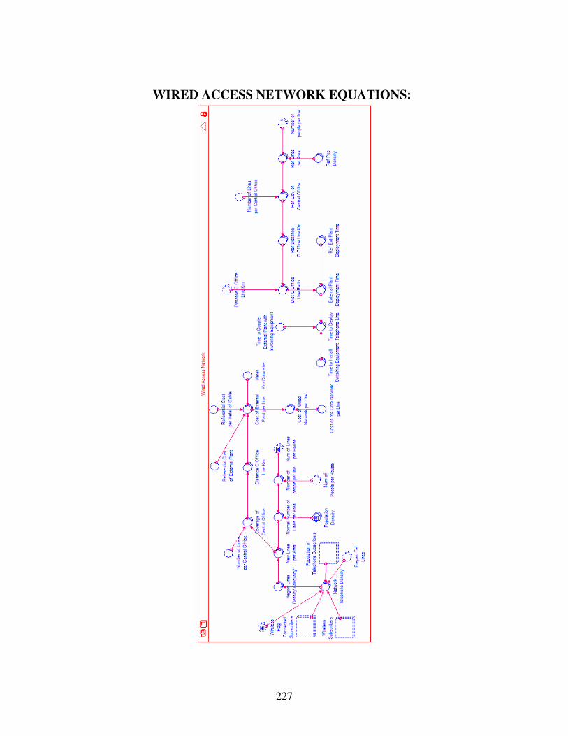
227

WIRED ACCESS NETWORK EQUATIONS:

228

Cost_of_External_Plant_per_Line[Region] = Referential_Cost_of_External_Plant+(Distance_C_Office__Line_Km[Region]*Meter_Km_Converter*Referential_Cost_per_Meter_of_Cable) Cost_of_the_Core_Network__per_Line = 40 Cost_of_Wired__Network_per_Line[Region] = Cost_of_External_Plant_per_Line[Region]+Cost_of_the_Core_Network__per_Line Coverage_of_Central_Office[Region] = Number_of_Lines__per_Central_Office/New_Lines__per_Area[Region] Distance_C_Office__Line_Km[Region] = SQRT(Coverage_of_Central_Office[Region]/(2*3.1416)) Dist_C_Office_Line_Ratio[Region] = Distance_C_Office__Line_Km[Region]/Ref_Distance__C_Office_Line_Km[Region] External_Plant__Deployment_Time[Region] = Ref_Ext_Plant_Deployment_Time[Region]*Dist_C_Office_Line_Ratio[Region] Meter_Km_Converter = 1000 Network_Telephone_Density[Region] = ((Connected__Subscribers[Region]+Prepaid_Tel_Lines[Region])*(1-Wireless_Flag[Region])/Population_of_Telephone_Subscribers[Region])+(Wireless__Subscribers[Region]*Wireless_Flag[Region]/Population_of_Telephone_Subscribers[Region]) New_Lines__per_Area[Region] = Normal_Number_of_Lines_per_Area[Region]*Region_Lines_Density_Adequacy[Region] Normal_Number_of_Lines_per_Area[Region] = Population__Density[Region]/Number_of__people_per_line_[Region] Number_of_Lines__per_Central_Office = 5000 Number_of__people_per_line_[Region] = Num_of_People_per_House[Region]/Num_of_Lines_per_House[Region] Population__Density[Urban] = 284 Population__Density[Rural] = 19 Referential_Cost_of_External_Plant = 150 Referential_Cost_per_Meter_of_Cable = 0.10 Ref_Cov_of_Central_Office[Region] = Number_of_Lines__per_Central_Office/Ref_Lines_per_Area[Region] Ref_Distance__C_Office_Line_Km[Region] = SQRT(Ref_Cov_of_Central_Office[Region]/(2*3.1416)) Ref_Ext_Plant_Deployment_Time[Region] = 12 Ref_Lines_per_Area[Region] = Ref_Pop_Density[Region]/Number_of__people_per_line_[Region] Ref_Pop_Density[Urban] = 284 Ref_Pop_Density[Rural] = 284 Time_to_Couple_External_Plant_with_Switching_Equipment = 1

229

Time_to_Deploy_Telephone_Line[Region] = IF(External_Plant__Deployment_Time[Region]>=Time_to_Install_Switching_Equipment[Region])THEN(External_Plant__Deployment_Time[Region]+Time_to_Couple_External_Plant_with_Switching_Equipment)ELSE(Time_to_Install_Switching_Equipment[Region]+Time_to_Couple_External_Plant_with_Switching_Equipment) Time_to_Install_Switching_Equipment[Urban] = 8 Time_to_Install_Switching_Equipment[Rural] = 18 Region_Lines_Density_Adequacy[Region] = GRAPH(Network_Telephone_Density[Region]) (0.00, 5.00), (0.1, 4.75), (0.2, 4.28), (0.3, 3.52), (0.4, 2.46), (0.5, 1.92), (0.6, 1.64), (0.7, 1.42), (0.8, 1.26), (0.9, 1.12), (1, 1.00)

230

WIRELESS ACCESS NETWORK EQUATIONS:

231

Avg_Mobile_Users_per_Base_Station[Region](t) = Avg_Mobile_Users_per_Base_Station[Region](t - dt) + (A_M_U__Growth[Region]) * dt INIT Avg_Mobile_Users_per_Base_Station[Region] = Wless_Lines_inside_Normal_Cell[Region]*Mobility_Offered[Region] INFLOWS: A_M_U__Growth[Region] = (Wless_Lines_inside_Normal_Cell[Region]-Avg_Mobile_Users_per_Base_Station[Region])/Avg_MUBS_Time Avg_Wireless_Lines_per_Base_Station[Region](t) = Avg_Wireless_Lines_per_Base_Station[Region](t - dt) + (AWLBS_Growth[Region]) * dt INIT Avg_Wireless_Lines_per_Base_Station[Region] = Actual_Wless_Lines_per_BS[Region] INFLOWS: AWLBS_Growth[Region] = (Actual_Wless_Lines_per_BS[Region]-Avg_Wireless_Lines_per_Base_Station[Region])/Avg_WLBS_Time Wireless__Subscribers[Region](t) = Wireless__Subscribers[Region](t - dt) + (MS_Growth[Region] - MS_Reduction[Region]) * dt INIT Wireless__Subscribers[Region] = 0 INFLOWS: MS_Growth[Region] = (Connecting_Rate[Region]+P_Phone_C_Rate[Prepaid_Phone, Region]*Lines_per_VAS_Users)*Wireless_Flag[Region] OUTFLOWS: MS_Reduction[Region] = (Connected__Subscribers__Attrition_Rate[Region]+VAS_Users_Attrition[Prepaid_Phone, Region]*Lines_per_VAS_Users)*Wireless_Flag[Region] Access_to_Electricity[Urban] = 0.98 Access_to_Electricity[Rural] = 0.5 Actual_Area_of_Cell[Region] = (Max_Area_of_Cell+Area__Adequacy[Region]*(Indicated_Area_of__Cell[Region]-Max_Area_of_Cell)) Actual_Wless_Lines_per_BS[Region] = Actual_Wless_Lines_per_BS_Indicated[Region]+Area__Adequacy[Region]*(Max_Wless_Lines_per_Base_Station-Actual_Wless_Lines_per_BS_Indicated[Region]) Actual_Wless_Lines_per_BS_Indicated[Region] = Actual_Area_of_Cell[Region]*New_Lines__per_Area[Region] Avg_MUBS_Time = 100 Avg_WLBS_Time = Avg_MUBS_Time Costs_of_Subscriber_Units_per_Line[Region] = Cost_of_Subscriber_Units[Region]/Actual_Wless_Lines_per_BS[Region] Cost_of_a_Base_Station = 150000 Cost_of_B_Station_per_Wless_Line[Region] = Cost_of_a_Base_Station/(Actual_Wless_Lines_per_BS[Region])

232

Cost_of_Core_Network_and_B_Station_per_Wless_Line[Region] = Cost_of_B_Station_per_Wless_Line[Region]+Cost_of_the_Core_Network__per_Line Cost_of_Normal_Subscriber_Unit = 50 Cost_of_Power_Supply[Region] = (Wless_Lines_inside_Normal_Cell_without_electricity[Region]+Wless_Lines_outside_Normal_Cell_without_electricity[Region])*Cost_of__Solar_Panel Cost_of_Special_Subscriber_Unit = 400 Cost_of_Subscriber_Units[Region] = Total_Cost_of_Special_Subscriber_Units[Region]+Total_Cost_of__Normal_Subscriber_Units[Region]+Cost_of_Power_Supply[Region] Cost_of_Wireless__Telephone_Line[Region] = Cost_of_Core_Network_and_B_Station_per_Wless_Line[Region]+Costs_of_Subscriber_Units_per_Line[Region] Cost_of__Solar_Panel = 500 Fraction_of_Mobile_Subscribers[Region] = Wireless__Subscribers[Region]*Share_of__Mobile_Users_per_B_Station[Region]/Total_Phone_Lines[Region] Fraction_of_Mobility_offered[Region] = Wless_Lines_inside_Normal_Cell[Region]*Mobility_Offered[Region]/Actual_Wless_Lines_per_BS[Region] Indicated_Area_of__Cell[Region] = Max_Wless_Lines_per_Base_Station/New_Lines__per_Area[Region] Max_Area_of_Cell = (Max_Radio__of_Cell^2)*3.1416 Max_Radio__of_Cell = 30 Max_Wless_Lines_per_Base_Station = 5000 Mobility_Offered[Region] = IF(Cost_of_Normal_Subscriber_Unit < 100) THEN (Wireless_Flag[Region]*1) ELSE (0) Normal_Area__of_Cell = (Normal_Radio__of_Cell^2)*3.1416 Normal_Radio__of_Cell = 5 Share_of__Mobile_Users_per_B_Station[Region] = Avg_Mobile_Users_per_Base_Station[Region]*Mobility_Offered[Region]/Avg_Wireless_Lines_per_Base_Station[Region] Total_Cost_of_Special_Subscriber_Units[Region] = Cost_of_Special_Subscriber_Unit*Wless_Lines_outside_Normal_Cell[Region] Total_Cost_of__Normal_Subscriber_Units[Region] = Cost_of_Normal_Subscriber_Unit*Wless_Lines_inside_Normal_Cell[Region] Total_Phone_Lines[Region] = Connected__Subscribers[Region]+VAS_Users[Prepaid_Phone,Region]+VAS_Users[Virtual_Telephony,Region] Wless_Lines_inside_Normal_Cell[Region] = Actual_Wless_Lines_per_BS[Region]-Wless_Lines_outside_Normal_Cell[Region] Wless_Lines_inside_Normal_Cell_without_electricity[Region] = Wless_Lines_inside_Normal_Cell[Region]*(1-Access_to_Electricity[Region])

233

Wless_Lines_outside_Normal_Cell[Region] = New_Lines__per_Area[Region]*((Actual_Area_of_Cell[Region]-Normal_Area__of_Cell)*Outside_Cell_Wless_Lines_Adequacy[Region]) Wless_Lines_outside_Normal_Cell_without_electricity[Region] = (1-Access_to_Electricity[Region])*Wless_Lines_outside_Normal_Cell[Region] Area__Adequacy[Region] = GRAPH(Max_Area_of_Cell/Indicated_Area_of__Cell[Region]) (1.00, 0.00), (1.00, 0.215), (1.00, 0.425), (1.00, 0.615), (1.00, 0.74), (1.00, 0.84), (1.01, 0.91), (1.01, 0.96), (1.01, 0.985), (1.01, 1.00), (1.01, 1.00) Outside_Cell_Wless_Lines_Adequacy[Region] = GRAPH(Actual_Area_of_Cell[Region]/Normal_Area__of_Cell) (1.00, 0.00), (1.00, 0.285), (1.01, 0.485), (1.01, 0.625), (1.02, 0.735), (1.02, 0.825), (1.03, 0.885), (1.03, 0.935), (1.04, 0.975), (1.04, 0.995), (1.05, 1.00)

234

TELECOM POLICIES EQUATIONS:

235

Market_Price[Region](t) = Market_Price[Region](t - dt) + (Price_Adjustment[Region]) * dt INIT Market_Price[Region] = Referential_Market_Price[Region] INFLOWS: Price_Adjustment[Region] = (Indicated_Price[Region]-Market_Price[Region])/Time_to__Adjust_Price[Region] M_Rental_Fee[Region](t) = M_Rental_Fee[Region](t - dt) + (MRF_Growth[Region]) * dt INIT M_Rental_Fee[Region] = M_Rental_Fee_Indicated_[Region] INFLOWS: MRF_Growth[Region] = (M_Rental_Fee_Indicated_[Region]-M_Rental_Fee[Region])/MRF_Adj_Time Universal_Service__Obligation(t) = Universal_Service__Obligation(t - dt) + (USO_Growth) * dt INIT Universal_Service__Obligation = USO_Referential INFLOWS: USO_Growth = (Universal_Service_Obligation_Indicated-Universal_Service__Obligation)/USO_Adj_Time USO_Policy(t) = USO_Policy(t - dt) + (USO_Policy_Adjustment) * dt INIT USO_Policy = 0 INFLOWS: USO_Policy_Adjustment = (Policy_Start_Indicated-USO_Policy)/Time_to__Implement_Policy VAS_Investment_Policy(t) = VAS_Investment_Policy(t - dt) + (VAS_Inv_Growth) * dt INIT VAS_Investment_Policy = VAS_Investment_Policy_Indicated INFLOWS: VAS_Inv_Growth = (VAS_Investment_Policy_Indicated-VAS_Investment_Policy)/VAS_Inv_A_T Indicated_Price[Region] = Market_Clearing_Adequacy[Region]*Referential_Market_Price[Region] Market_Price_Flag = 0 MRF_Adj_Time = 3 M_Rental_Fee_Indicated_[Urban] = Referential_Monthly__Rental[Urban] M_Rental_Fee_Indicated_[Rural] = Referential_Monthly__Rental[Rural] Policy_Start_Indicated = IF(Supplied__Telephone_Lines[Urban]>=Demanded_Telephone__Lines[Urban] AND Region_Telephone_Density[Urban]>=0.01)THEN(1)ELSE(0) Referential_Market_Price[Region] = Referential_Price[Region]

236

Referential_Monthly__Rental[Urban] = Referential_Price[Urban]*(1-Market_Price_Flag)+Market_Price[Urban]*Market_Price_Flag Referential_Monthly__Rental[Rural] = Referential_Price[Rural]+0*Market_Price[Rural]*Market_Price_Flag Referential_Price[Urban] = 1 Referential_Price[Rural] = 1 Referential_Time_to_Adjust_Market_Price = 60 Time_to__Adjust_Price[Region] = Referential_Time_to_Adjust_Market_Price*(1+Market_Clearing_Adequacy[Region]) Time_to__Implement_Policy = 12 Universal_Service_Obligation_Indicated = IF(USO_Policy > 0.9 AND USO_Improved_Flag = 1)THEN(USO_Improved)ELSE(USO_Indicated) USO_Adj_Time = 3 USO_Improved = 0.45 USO_Improved_Flag = 0 USO_Indicated = IF(TIME < 48) THEN (USO_Referential+0.215*0) ELSE (USO_Referential) USO_Referential = 0.035 VAS_Investment_Policy_Indicated = VAS_Investment_Referential VAS_Investment_Referential = 0 VAS_Inv_A_T = 30 Market_Clearing_Adequacy[Region] = GRAPH(Supplied__Telephone_Lines[Region]/Demanded_Telephone__Lines[Region]) (0.00, 10.0), (0.2, 7.35), (0.4, 5.20), (0.6, 3.55), (0.8, 2.25), (1.00, 1.00), (1.20, 0.45), (1.40, 0.1), (1.60, 0.1), (1.80, 0.05), (2.00, 0.005)

THE IMPACT OF UNIVERSAL SERVICE … IMPACT OF UNIVERSAL SERVICE OBLIGATIONS AND OTHER EXTERNAL AND...

Documents

Transcript of THE IMPACT OF UNIVERSAL SERVICE … IMPACT OF UNIVERSAL SERVICE OBLIGATIONS AND OTHER EXTERNAL AND...