DI

SC

US

SI

ON

P

AP

ER

S

ER

IE

S

Forschungsinstitut zur Zukunft der ArbeitInstitute for the Study of Labor

The Impact of Training on Productivity and Wages: Firm Level Evidence

IZA DP No. 4731

January 2010

Jozef KoningsStijn Vanormelingen

The Impact of Training on Productivity

and Wages: Firm Level Evidence

Jozef Konings KU Leuven, BEPA, European Commission

and IZA

Stijn Vanormelingen HU Brussels and LICOS, KU Leuven

Discussion Paper No. 4731 January 2010

IZA

P.O. Box 7240 53072 Bonn

Germany

Phone: +49-228-3894-0 Fax: +49-228-3894-180

E-mail: iza@iza.org

Any opinions expressed here are those of the author(s) and not those of IZA. Research published in this series may include views on policy, but the institute itself takes no institutional policy positions. The Institute for the Study of Labor (IZA) in Bonn is a local and virtual international research center and a place of communication between science, politics and business. IZA is an independent nonprofit organization supported by Deutsche Post Foundation. The center is associated with the University of Bonn and offers a stimulating research environment through its international network, workshops and conferences, data service, project support, research visits and doctoral program. IZA engages in (i) original and internationally competitive research in all fields of labor economics, (ii) development of policy concepts, and (iii) dissemination of research results and concepts to the interested public. IZA Discussion Papers often represent preliminary work and are circulated to encourage discussion. Citation of such a paper should account for its provisional character. A revised version may be available directly from the author.

IZA Discussion Paper No. 4731 January 2010

ABSTRACT

The Impact of Training on Productivity and Wages: Firm Level Evidence*

This paper uses firm level panel data of firm provided training to estimate its impact on productivity and wages. To this end the strategy proposed by Ackerberg, Caves and Frazer (2006) for estimating production functions to control for the endogeneity of input factors and training is applied. The productivity premium for a trained worker is estimated at 23%, while the wage premium of training is estimated at 12%. Our results give support to recent theories that explain work related training by imperfect competition in the labor market. JEL Classification: J24, J31, L22 Keywords: training, production functions, human capital Corresponding author: Jozef Konings Katholieke Universiteit Leuven Hogenheuvelcollege Naamsestraat 69 3000 Leuven Belgium E-mail: Joep.Konings@econ.kuleuven.be

* We would like to thank Filip Abraham, Anneleen Forrier, Lisa George, Johannes Van Biesebroeck, Patrick Van Cayseele, Bart Cockx, Marton Csillag, Jan De Loecker, Steve Pischke, Bee Roberts and Vitor Gaspar for useful comments and suggestions. This paper has benefited from presentations at the Belgian Day for Labour Economists in Louvain-la-Neuve, the HU Brussel Research Seminar Series, the Panel Data Conference in Bonn and the EARIE conference in Ljubljana.

1 Introduction

In recent years trade unions, employers and policy makers have emphasized the

importance of skill upgrading of workers and life long learning in order to cope

with increased pressures induced by technological change and globalization (e.g.;

European Commission, 2007). While there exists a large literature showing that

the accumulation of human capital through the general education system plays

a crucial role in explaining long run income di¤erences between rich and poor

countries, much less work exists on the e¤ects of training provided by �rms,

often requiring speci�c skills from their workers.

In his seminal work, Becker(1964) made a distinction between �rm speci�c

and general training. General training results in skills that are equally applica-

ble at other �rms while skills acquired through �rm speci�c training are lost

when the trained worker leaves the �rm that provided training. Under perfect

competition in the labor market, workers should pay for costs of general training

and recoup these costs by earning higher wagers. When training is speci�c, �rms

pay (part of) the training costs1 . However, Acemoglu and Pischke (1998, 1999a,

1999b) point out that in numerous cases �rms provide and pay for training that

is general in nature. They show how this can be explained by labor market

imperfections. In particular, a necessary condition for �rms to pay for general

training is that wages increase less steeply in training than productivity. This

is referred to as a compressed wage structure which can be caused by frictions

in the labor market such as search costs, informational asymmetries, e¢ ciency

wages and labor market institutions such as unions or the presence of minimum

wage laws. With a compressed wage structure, training increases the marginal

product of labor more than wages, which creates incentives for the �rm to invest

in training.

While there exists substantial evidence that general education increases

wages2 and productivity of workers, there is hardly any work that studies the

impact of work related training on �rm level productivity and wages. Moretti

1 In fact, with �rm speci�c training it is more e¢ cient if �rms and workers share the costsand bene�ts of training. Wages of workers increase after speci�c training above the level theycould earn elsewhere but lower than their marginal product which reduces both the probabilitythey quit the �rm and the propability they are laid o¤.

2Card (1999), for instance, summarizes various studies and concludes that the impact ofa year of schooling on wages is about 10%.

2

(2004) focuses on plant level productivity gains from education, but he has no

data on �rm provided training. He �nds that plants operating in cities that

experience a large increase in the share of college graduates have higher pro-

ductivity gains than in cities that have a lower increase in college graduates,

but these productivity gains are o¤set by wage increases. Bartel (1995) studies

how �rm provided training a¤ects wage pro�les of workers and job performance

scores in one large �rm and �nds that training has a positive e¤ect. Dearden,

Reed and Van Reenen (2006) analyze the link between training, wages and pro-

ductivity at the sector level using a panel of British industries. They �nd that

raising the proportion of workers in an industry who receive training by one

percentage point increases value added per worker in the industry by 0.6% and

average wages by 0.3%.

Our paper makes several contributions to the literature. First, we make use

of �rm level data on training. Belgian �rms are obliged by law to submit a

supplement to their annual income statement which contains information on

various elements of training, such as the proportion of workers that received

training, the number of hours they were trained and the cost of training to the

�rm. This data allows us to measure the impact of training on both wages

and productivity at the �rm level and we can infer whether trained workers

are paid the value of their marginal product. By focusing on �rm level data

we are able to avoid possible aggregation biases and hence capture the e¤ects

of training more precisely. Second, the analysis at the �rm level allows us to

control for the endogeneity of training. To this end we estimate the production

function using an estimation strategy recently introduced by Ackerberg, Caves

and Frazer (2006) which allows us to control for the endogeneity of input factors.

In addition, the production function estimates provide us with a measure of

unobserved worker ability which we include in the wage equation to retrieve

a consistent estimate for the impact of training on wages. Third, we are able

to explore various dimensions of the data set. Because of the large number of

observations, we can analyze di¤erences between narrowly de�ned sectors with

respect to the impact of training on �rm performance and relate the incidence

of training with quit and dismissal rates.

Our main �ndings can be summarized as follows. Training has a positive im-

pact on productivity and wages. The marginal product of a trained worker is on

average 23% higher than that of an untrained worker while wages only increase

3

with 12% in response to training and the di¤erence is statistically signi�cant3 .

This �nding is consistent with recent theories that explain �rm provided train-

ing by models with imperfect competition in the labor market and is robust

against di¤erent kinds of speci�cations and estimation strategies. Among the

di¤erent manufacturing sectors, largest productivity gains can be found in the

Chemicals and Rubber & Plastic industries. Finally we provide some indicative

evidence that the observed training is general in nature.

The next section gives the empirical framework we use and we describe our

estimation strategy in Section 3. We give an overview of the dataset in Section

4. Results are reported in Section 5 and Section 6 makes a distinction between

�rm speci�c and general training. Finally, we conclude in Section 7.

2 Empirical Framework

We infer the impact of training on both wages and productivity by applying a

framework used by Hellerstein et al. (1999). The idea is to estimate both a

wage equation and a production function to compare gains in wages with the

gains in productivity that may arise in response to training. In competitive

labor markets, returns from human capital formation accrue to workers in the

form of wages and the productivity premium of a trained worker equals its

wage premium4 . While most studies that estimate wage di¤erentials between

di¤erent types of workers rely on individual level data, this option is not available

to estimate productivity di¤erentials since it is hard if not impossible to �nd

individual level output data. Consequently we will rely on rich �rm level data

with information on the di¤erent kinds of characteristics of the workforce such

as the amount of training among others. The drawback is that we can only

estimate an average productivity and wage premium for trained workers and

can not capture heterogeneity in these premia across di¤erent workers.

3These productivity and wage premia drop to 17% and 11% respectively when controllingfor worker heterogeneity.

4The framework has been applied among others by Jones (2001) to examine the impact ofeducation on earnings and productivity and by Hellerstein and Neumark (1999) to estimatewhether the wage gap between men and women can be explained by productivity di¤erentials.Frazer (2001) uses the methodology to �nd unbiased estimates for the impact of education onwages. More recently Van Biesebroeck (2007) applies the framework to estimate returns tohuman capital, including training, on both productivity and wages for some African countriesand Dearden et al. (2006) estimate the impact of training on wages and productivity for apanel of UK industries.

4

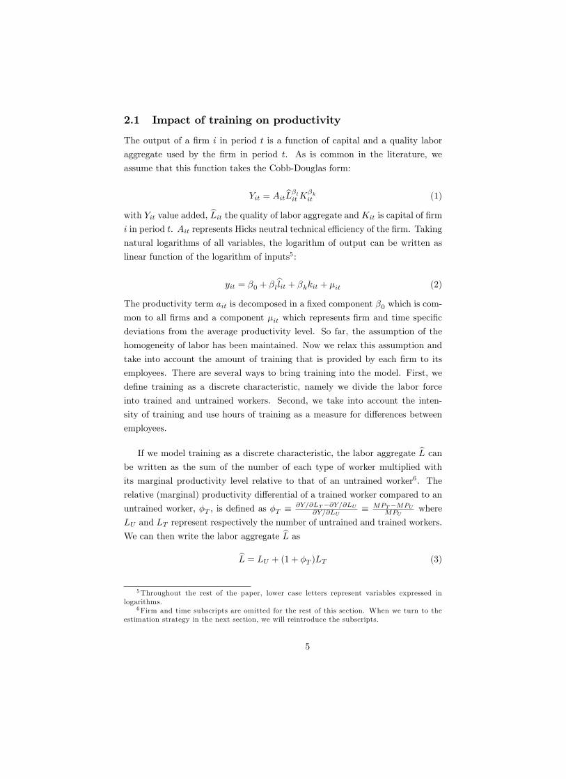
2.1 Impact of training on productivity

The output of a �rm i in period t is a function of capital and a quality labor

aggregate used by the �rm in period t. As is common in the literature, we

assume that this function takes the Cobb-Douglas form:

Yit = AitbL�litK�kit (1)

with Yit value added, bLit the quality of labor aggregate and Kit is capital of �rm

i in period t. Ait represents Hicks neutral technical e¢ ciency of the �rm. Taking

natural logarithms of all variables, the logarithm of output can be written as

linear function of the logarithm of inputs5 :

yit = �0 + �lblit + �kkit + �it (2)

The productivity term ait is decomposed in a �xed component �0 which is com-

mon to all �rms and a component �it which represents �rm and time speci�c

deviations from the average productivity level. So far, the assumption of the

homogeneity of labor has been maintained. Now we relax this assumption and

take into account the amount of training that is provided by each �rm to its

employees. There are several ways to bring training into the model. First, we

de�ne training as a discrete characteristic, namely we divide the labor force

into trained and untrained workers. Second, we take into account the inten-

sity of training and use hours of training as a measure for di¤erences between

employees.

If we model training as a discrete characteristic, the labor aggregate bL canbe written as the sum of the number of each type of worker multiplied with

its marginal productivity level relative to that of an untrained worker6 . The

relative (marginal) productivity di¤erential of a trained worker compared to an

untrained worker, �T , is de�ned as �T �@Y=@LT�@Y=@LU

@Y=@LU� MPT�MPU

MPUwhere

LU and LT represent respectively the number of untrained and trained workers.

We can then write the labor aggregate bL asbL = LU + (1 + �T )LT (3)

5Throughout the rest of the paper, lower case letters represent variables expressed inlogarithms.

6Firm and time subscripts are omitted for the rest of this section. When we turn to theestimation strategy in the next section, we will reintroduce the subscripts.

5

This functional form assumes that trained and untrained workers are perfect

substitutes and a �rm makes its training decisions solely based on productivity

di¤erences between employees and the cost of training. We can rewrite bL as:bL = L(1 + �T LTL ) (4)

Here L represents the total number of employees and is by de�nition the sum of

both trained and untrained workers. Consequently, LTL is the fraction of trained

workers in the labor force. Substituting Equation (4) in Equation (2) gives:

y = �0 + �ll + �l ln

�1 + �T

LTL

�+ �kk + � (5)

or when �TLTL is small, this can be approximated by

y = �0 + �ll + �l�TLTL+ �kk + � (6)

In principle we can infer the training premium from a linear regression of out-

put on capital, labor and the share of trained workers in total employment. A

positive coe¢ cient on the share of trained workers indicates that the marginal

product of a trained worker is higher compared to the marginal product of an

untrained worker. The precise magnitude of the average productivity premium

can be retrieved by dividing the training coe¢ cient by the labor coe¢ cient7

�l. In Appendix A we generalize the approach to include multiple character-

istics of the workforce. Note that we discard any heterogeneity in the impact

of training across workers and we implicitly assume all trained workers have a

similar productivity increase. We will interpret our estimates for the produc-

tivity premium more as an average e¤ect of training on productivity. Moreover,

we assume there exists only a direct e¤ect of training on the productivity of the

trained worker himself. However, training may also increase productivity of un-

trained coworkers through spillover e¤ects (Blundell et al. 1999). Unfortunately,

it is di¢ cult to identify these spillover e¤ects without individual level data or

stringent functional form assumptions8 . Consequently we choose not to control

for spillovers to other workers. Our point estimates should be interpreted with

caution since these possible e¤ects are attributed to the estimated productivity

7This is because the impact of an extra trained worker also depends on the importance oflabor in the production function: @ lnY

@LT= �T �l.

8For example when the spillover e¤ect is a linear function of the share of trained employees,one could infer the spillover coe¢ cient from adding the share of trained employees squared inthe labor aggregate.

6

premium. Note that both inputs and the number of trained workers are likely

to be correlated with elements of the unobserved productivity � of a �rm which

complicates the identi�cation of the coe¢ cients. We turn back to this issue in

Section 3.

So far we have de�ned training as a discrete characteristic. Either a worker

has received training over the period or he has not. However, this is a sim-

pli�cation since there exists considerable variation in the amount of training

each worker received. For example, the �rm speci�c average training hours

per worker trained ranges from less than 1 hour to more than 300 hours. To

take into account these variations in training intensity we include training as

a continuous variable instead of a binary variable. Frazer (2001) shows how

to derive the labor aggregate in a production function consistent with Mincer

(1974) when the characteristic that di¤erentiates the labor force is a continuous

variable9 . In our baseline model, workers di¤er only by the amount of training

they received. A typical equation in the style of Mincer (1974) that explains

the earnings of individual j as a function of the amount of training he obtained,

looks like:

ln(Wj) = �0 + �TTj + �j (7)

which means that the average wage bill of a �rm can be written asP

j exp(�0+

�TTj + �j). Here Tj represents the amount of training hours worker j has

received. Frazer (2001) proves that if the �rm is maximizing its pro�ts, the

labor term in the production function should have the same form as the wage

bill, i.e. bL =Pj exp(�1+ �TTj) and the production function can be written as

follows:

Y = A(Xj

exp(�1 + �TTj))�lK�k (8)

where �T measures how the contribution of an individual worker j to the aggre-

gate labor term varies with the amount of training he received (@ ln(bL)=@Tj =�T ). Taking natural logarithms, this can be rewritten as:

y = �l�1 + �l ln(Xj

exp(�TTj)) + �kk + a (9)

9To be precise, Frazer (2001) derives this result under the assumption of perfect compe-tition in the labor market. Intuitively, if a �rm is pro�t maximizing and acts as a price takerin the labor market, di¤erences in wages should re�ect di¤erences in marginal products andthe aggregate labor term in the production function should have exactly the same functionalform as the wage equation. However, with for example labor market frictions, productivitypremia do not necessarily equal wage premia and we have to assume that the functional formof the labor aggregate in the production function is the same as the functional form of thewage equation.

7

A �rst-order Taylor approximation of the labor term results in a loglinear equa-

tion that can be estimated (cf. Frazer, 2001). The logarithm of output is a

function of the logarithm of the number of workers and capital and the average

training hours of all workers in a particular �rm:

y = ��0 + �ll + �l�TT + �kk + � (10)

The coe¢ cient on average training intensity �T measures how the labor ag-

gregate changes with training intensity. The impact of training on output

depends also on the importance of labor in the production function �l, i.e.

@y=@T = �l�T , which represents the percentage changes in output in response

to variations in average training intensity of the workforce.

2.2 Impact of training on wages

We derive wage equations similar to Equations (6) and (10). The wage equation

will be more descriptive than the structural productivity equation. Again, we

�rst build up the empirical framework de�ning training to be a discrete char-

acteristic. Second, we take into account the variations in training intensity in

terms of training hours across trained employees.

To measure wage di¤erentials between trained and untrained employees, we

apply �rm-level wage equations as in Hellerstein et al. (1999). We de�ne a wage

equation in the style of Mincer (1974) for individual j:

Wj =WUDj;U +WTDj;T

where Wj is the wage of individual j. WU and WT are the average wages of

an untrained and trained employee respectively and Dj;U and Dj;T represent

a dummy equal to one if employee j is untrained or trained respectively. By

summing over all employees at a �rm, the total wage bill of a �rm equals by

de�nition the sum of the wages of trained and untrained employees multiplied

by respectively the number of trained and untrained employees active in the

�rm. This expression can be rewritten as

WL =WULU +WTLT =WUL+ �TWULT =WUL(1 + �TLTL) (11)

where �T = WT�WU

WUrepresents the relative wage premium for a trained em-

ployee compared to an untrained one. Dividing both sides by the number of

8

employees and taking logs of Equation (11) one obtains

w = wU + ln

�1 + �T

LTL

�� wU + �T

LTL

(12)

Where the last step follows from the fact that ln(1+x) can be approximated by x

if x is small. This equation at the �rm level is consistent with the individual level

Mincer (1974) wage equations. Under perfect competition in the labor market,

wages do not vary systematically across �rms and regressing the average wage on

a constant and the share of trained employees will give a consistent estimate for

the relative wage premium of trained employees. However, we will include the

capital intensity and total factor productivity in the estimation equation in order

to allow for imperfectly competitive labor markets and unobserved di¤erences

in labor quality which should be re�ected in total factor productivity. Adding a

vector of control variables X and an additive error term10 to equation (12) we

get:

w = wU + �TLTL+X + " (13)

which can be estimated by applying a least squares estimator11 .When we �nd

a positive association between the average wage at the �rm and the share of

trained workers this is an indication of a positive wage premium for trained

workers. More precise, the coe¢ cient on the share of trained workers will rep-

resent an average wage premium of a trained worker compared to an untrained

worker12 .

The derivation of a �rm level wage equation when we take into account

variations in training intensity across trained workers is similar to the derivation

of the labor aggregate in the production function of the previous section. The

average wage in a �rm can be written as:

w = wU + �TT (14)

10Note that Equation (12) is not a behavioral equation, but simply de�nes the averagewage to be a function of the wages of each di¤erent type of worker. The error term that weadd can represent measurement error, variation across �rms in wages across �rms unrelatedto productivity di¤erences, regional di¤erences in labor market conditions, . . .

11Again, we refer to Appendix A for the inclusion of multiple workforce characteristics inthe wage equation.

12Similar to the derivation of the productivity premium, we have assumed the wage pre-mium is constant and equal for all workers that receive training. This seems a quite harshassumption and we interpret the coe¢ cient on the share of trained workers more as an averageimpact of training on wages.

9

Where T represents average training costs per employee, �T measures how wage

premiums change with the intensity of training (@w=@T ) and wU is the average

wage of a worker that received no training at all. Again we add an additive

error term and control variables:

w = wU + �TT +X + " (15)

which can be estimated using ordinary least squares.

3 Estimation strategy

One needs to be careful in estimating the production function in Equation (6)

since inputs are likely to be correlated with the unobserved productivity term.

In this section, we describe in detail how we solve this problem. Recall the

production function derived in the previous section:

yit = �0 + �llit + �l�TLT;itLit

+ �kkit + !it + �it (16)

where the unobserved productivity term �it is divided into two components,

namely !it and �it. Unobservables that are not seen by the �rm at the moment

when it makes its input decisions are represented by the mean zero error term

�it. Consequently, inputs will be uncorrelated with this unobservable. An exam-

ple is an unexpected machine breakdown or strike. Also measurement error in

the output variable can be incorporated in �it: The !it represents productivity

unobserved by the econometrician, but observed by the �rm before making its

input decisions. Examples include managerial ability, expected machine break-

downs, technological progress, worker ability,. . . As such the input choices are

likely to be correlated with the unobserved error term !it and estimating Equa-

tion (16) with OLS will generate biased point estimates. This simultaneity bias

has been documented �rst by Marschak and Andrews (1944)13 . Note that also

the unobserved (by the econometrician) ability of employees or labor quality is

likely to be included in the productivity term !it. If �rms tend to provide train-

ing to the most able employees, for example because they are faster learners and

therefore require a smaller training investment, the estimated coe¢ cient on the

training variable will be upward biased.

13For an overview of the outstanding issues in estimating production functions, we refer toAckerberg et al. (2005).

10

Olley and Pakes (1996) o¤er a solution to the endogeneity problem. They

set up a dynamic model and derive the productivity !it to be a function of in-

vestment and capital. As such, productivity can be proxied by a nonparametric

function of investment and capital and can be controlled for in the estimation

of Equation (16). The drawback of this method is that only observations with

positive investment levels can be used in the estimation. Levinsohn and Petrin

(2003) overcome this problem by using material inputs instead of investment

in the estimation of productivity !it. Both methods assume that labor has no

dynamic implications and hence the choice of labor in year t has no impact on

future pro�ts. This implies among others that there can be no hiring and �ring

costs and that �rms can choose each period the optimal amount of labor at a

given wage rate without any limitations. Given that Belgium is a highly union-

ized country with rigid labor markets and that there exist considerable costs in

laying o¤ employees, we will relax this assumption. Moreover, Ackerberg, Caves

and Frazer (2006) note that identifying the coe¢ cients on labor and materials

using the Levinsohn and Petrin (2003) or Olley and Pakes (1996) methodology

could be problematic due to collinearity issues. For these reasons, we will follow

the methodology proposed by Ackerberg, Caves and Frazer (2006) to correct for

the simultaneity bias, which we will discuss now in more detail.

We keep the timing assumption made in Levinsohn and Petrin (2003) and

Olley and Pakes (1996) about the capital accumulation function:

kit = (1� �)kit�1 + iit�1 (17)

with iit�1 investment decided in period t�1 which only enters the capital stockin year t. Intuitively, the expression means that it takes a full period to order

and install the new capital goods before they enter the production process. We

will use this assumption to identify the capital coe¢ cient in the second stage of

the estimation strategy since by de�nition the capital stock will be uncorrelated

with the part of productivity in year t, unforeseen in year t � 1. Furthermorewe assume that !it follows a �rst-order Markov process:

p (!itjIit�1) = p (!itj!it�1) (18)

where Iit is the information set of �rm i at period t � 1. This assumptionmeans that �rms�expectations of future productivity only depend on current

productivity. We assume material input to be chosen after labor input and

training which seems plausible for an economy with rigid labor markets like

11

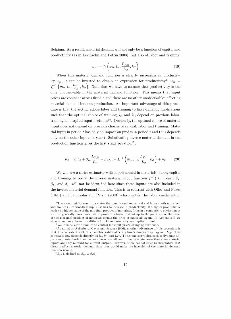
Belgium. As a result, material demand will not only be a function of capital and

productivity (as in Levinsohn and Petrin 2003), but also of labor and training:

mit = ft

�!it; lit;

LT;itLit

; kit

�(19)

When this material demand function is strictly increasing in productiv-

ity !it, it can be inverted to obtain an expression for productivity14 !it =

f�1t

�mit; lit;

LT;itLit

; kit

�. Note that we have to assume that productivity is the

only unobservable in the material demand function. This means that input

prices are constant across �rms15 and there are no other unobservables a¤ecting

material demand but not production. An important advantage of this proce-

dure is that the setting allows labor and training to have dynamic implications

such that the optimal choice of training, lit and kit depend on previous labor,

training and capital input decisions16 . Obviously, the optimal choice of material

input does not depend on previous choices of capital, labor and training. Mate-

rial input in period t has only an impact on pro�ts in period t and thus depends

only on the other inputs in year t. Substituting inverse material demand in the

production function gives the �rst stage equation17 :

yit = �llit + �trLT;itLit

+ �kkit + f�1t

�mit; lit;

LT;itLit

; kit

�+ �it (20)

We will use a series estimator with a polynomial in materials, labor, capital

and training to proxy the inverse material input function f�1(:). Clearly �l,

�k, and �tr will not be identi�ed here since these inputs are also included in

the inverse material demand function. This is in contrast with Olley and Pakes

(1996) and Levinsohn and Petrin (2003) who identify the labor coe¢ cient in

14The monotonicity condition states that conditional on capital and labor (both untrainedand trained) , intermediate input use has to increase in productivity. If a higher productivityleads to a higher value of the marginal product of materials, �rms in a competitive environmentwill use generally more materials to produce a higher output up to the point where the valueof the marginal product of materials equals the price of materials again. In Appendix B weshow some more formal conditions for the monotonicity assumption to hold.

15We include year dummies to control for input prices changing over time.16As noted by Ackerberg, Caves and Frazer (2006), another advantage of this procedure is

that it is consistent with other unobservables a¤ecting �rm�s choices of lit; kit and LiT . Thisis because mit depends directly on lit; kit and LiT . These unobservables, such as dynamic ad-justment costs, both linear as non-linear, are allowed to be correlated over time since materialinputs are only relevant for current output. However, there cannot exist unobservables thatdirectly a¤ect material demand since they would make the inversion of the material demandfunction invalid.

17�tr is de�ned as �tr � �l�T

12

the �rst stage of the estimation strategy. Here, the �rst stage only serves to

separate �it from !it. Estimating the above equation gives a measure b�it forthe following term:

�it = �llit + �trLT;itLit

+ �kkit + !it (21)

which is in fact output net of the error term �it. The estimate b�it will be usedto identify the input coe¢ cients in the second stage. Since productivity !it is

assumed to follow a �rst-order Markov process, it can be written as follows:

!it = E [!itjIit�1] + �it (22)

= E [!itj!it�1] + �it= g(!it�1) + �it

where �it represents the innovation in productivity, namely the part of produc-

tivity in period t that was unforeseen by the �rm in period t � 1. Given thetiming assumption that the capital stock in period t was decided in period t�1,this leads to a �rst moment condition which will allow us to identify the capital

coe¢ cient:

E [�itjkit] = 0 (23)

Moreover, we assume that labor input and the amount of training do not

depend on the innovation in productivity. For the labor coe¢ cient, this is a

more strict assumption than usually applied. However, in the Belgian context

there are substantial labor adjustment costs such that labor is not freely variable

input18 . Concerning the training variable, several human resources managers

con�rmed that the amount of training provided to workers is mostly decided

one year in advance when making up the budget for the following year, which

makes the amount of training independent from the innovation in productivity,

�it. Consequently, the moment conditions to identify the labor and training

coe¢ cients in the second stage are19 :

18For example, the OECD Employment Protection Legislation for Belgium is among thehighest among the industrialized countries (higher scores indicate stricter regulation). Belgiumhas especially a high score for the notice and severence pay for individual dismissals, legislationconcerning collective dismissals and temporary employment (OECD 2007).

19These timing assumptions are relaxed in the robustness checks. Namely we will allowtraining and part of the labor stock to be correlated with the innovation in productivity.

13

E

24�itj kitlit

LT;it=Lit

35 = 0 (24)

In practice, we apply the �rst stage by non-parametrically regressing yiton the production inputs. This gives us an estimate b�it for �it = �llit +

�trLT;itLit

+�kkit+!it. Given a candidate value for the vector of input coe¢ cients

(�l; �k; �tr), we can compute b!it as follows:b!it = b�it � �llit � �trLT;itLit

� �kkit (25)

Next, we non-parametrically regress !it on !it�1. The residuals from this re-

gression b�it represent innovations in productivity, which are by assumption un-correlated with training, labor and capital. This renders the above moment

conditions and their sample analogue:

1

T

1

N

Xt

Xt

b�it0@ kit

litLT;it=Lit

1A (26)

and we compute the sample analogue for each (�l; �k; �tr) For each new candi-

date value of (�l; �k; �tr), we obtain new estimates for �it and we repeat this

procedure until Equation (26) is minimized.

Given the input coe¢ cients we found in the previous step, we �nd an estimate

for total factor productivity by applying Equation (25). We use this estimate in

the wage equation as control variable to pick up unobservables such as worker

ability that in�uence wages of the workers20 . When not controlled for, these

variables could cause our estimate for the wage premium to be biased since for

example more able workers are also more likely to receive training. Standard

errors for all coe¢ cients are obtained by using a bootstrap procedure with 500

replications. We apply a block bootstrap procedure such that the error term is

allowed to be heteroskedastic and correlated over time t, for a given �rm i but

is assumed to be independent over i.

20This is a similar strategy as applied in Frazer (2001).

14

4 Data Description

Data is obtained from the Bel�rst database. This database commercialized by

Bureau Van Dijck includes information about all Belgian �rms that need to �le

annually an income statement.21 We obtained an unbalanced panel for the pe-

riod 1997-2006 of both manufacturing and non-manufacturing �rms. We select

a number of key variables needed for estimation of the production function and

wage equation such as value added, number of employees (in full time equiv-

alents), labor costs, material costs and the capital stock. For manufacturing

sectors, these variables are de�ated using price de�ators at the 4 digit NACE

level from the European Statistical O¢ ce22 . For the non-manufacturing sectors

we use a NACE 2 digit price de�ator from the EU Klems database. In addition

to the aforementioned variables, Belgian �rms are obliged to report information

about formal training23 they provide to their employees. In particular, they have

to report the number of employees that followed some kind of formal training

as well as the hours spent on this training and the training costs. This allows us

to obtain a �rm-level measure of training for more than 170; 000 Belgian �rms

active in manufacturing and non-manufacturing sectors.

Table 1 provides some summary statistics of the dataset used. A Belgian �rm

active in the private sector employs on average 16:9 employees and generates a

turnover of around 10 million euro. It pays an average wage of around 35; 000

euro and the average labor productivity (= value added per employee) equals

63; 900 euro. The second and third column compare these �gures between �rms

that provided training to at least one employee in at least one year of the sample

period with �rms that have never trained an employee over the sample period.

By comparing columns (2) and (3) it can be seen that less than 10% of the �rms

have ever invested in training of one of their employees. These �rms are typically

larger in terms of both employment and turnover. Moreover they pay higher

wages and have a higher labor productivity. Surprisingly, �rms that provide

training to their employees have a lower capital/labor ratio than non-training

�rms, but this result changes when we control for other characteristics as we

will see below. In �rms that train their workers in a given period, more than

21These are all Belgian enterprises with the exclusion of one-man businesses.22For some 4 digit NACE sectors, price de�ators are not reported. Here we use the 3 digit

de�ator.23Formal training excludes training that takes place at the work�oor or self study. The

training has to take place at a seperate training room or work�oor especially developed fortraining activities. Training can take place inside or outside the �rm.

15

50% of the employees bene�t from this training and spent on average almost 40

hours on this training. The average cost of training an employee equals more

than 1; 500 euro.

Table 2 shows the results of the regression of di¤erent key variables on a

training dummy. This dummy equals 1 when a particular �rm provides training

to at least one of its employees in a given period and 0 otherwise. The dependent

variable is expressed in logarithms, such that the coe¢ cient on the training

dummy can be interpreted as a percentage di¤erence24 . The �rst column of

Table 2 shows the results of this exercise. A training �rm is more than twice as

large as a non-training �rm and pays gross wages that are 36% higher. Labor

productivity is also higher but the di¤erence is smaller than for labor costs. In

column (2), we control for the size of the �rm, that is we include the number of

employees as explanatory variable and in column (3), we also include NACE 4

digit dummies to control for sector characteristics. Now, labor productivity in

training �rms is 27% higher than in non-training �rms while labor costs are only

18% higher. Note that when controlling for industry characteristics and the size

of the �rm, training �rms have a higher capital-labor ratio than non-training

�rms.

There exists considerable variation in the amount of training across sectors.

This is illustrated in Table 3 where the percentage of �rms that provided training

to their employees in 2006 is shown. We also show the percentage of workers that

received some kind of (formal) training and the share of training costs in total

labor costs. These two measures are weighted averages, that is the total share of

trained workers in sector j equalsP

i LT;ijPi Lij

, where i is a �rm indicator. Likewise,

the share of training costs in total labor costs is the fraction of total training costs

in sector j divided by total labor costs in the sector. Despite that only slightly

more than 5% of the �rms provided training to at least one employee in 2006,

more than 30% of all employees received training. This is because training �rms

are much larger than non-training �rms as can be seen in Table 1. Training costs

make up almost 1% of total labor costs. In general, manufacturing �rms train

more than their non-manufacturing counterparts. The most training intensive

sectors include Manufacturing of Chemical Products, Telecommunications and

Electricity Sector. Least training can be found in sectors such as Agriculture,

Construction and Hotels & Restaurants.24Of course this is an approximation, certainly because for some variables, the di¤erence

between training and non-training �rms is quite large.

16

5 Results

This section presents the results of the empirical analysis. First, we estimate

productivity and wage premia for all sectors pooled together and for each sector

separately. Next we measure training as a continuous variable before moving to

some robustness checks. Finally we include other sources of worker heterogeneity

in the analysis, under the assumption of both perfect and imperfect substitution

between di¤erent types of workers.

5.1 General Results

Table 4 shows the results of estimating Equation (6) for all �rms active in all

sectors pooled together and for manufacturing and non-manufacturing sepa-

rately25 . The �rst column for each subsample (Total, Manufacturing and Non-

Manufacturing) reports the estimation results for the full sample by applying

ordinary least squares (OLS1)26 . Unfortunately, many �rms do not report ma-

terial costs27 such that the estimation methodology described in Section 3 can

only be applied to a subset of �rms. To allow comparison between the ordinary

least squares estimates and the estimates controlling for the endogeneity of in-

puts in the third column(ACF), we report in the second column results for least

squares estimation (OLS2) on this subset of �rms28 . The estimates reported

in column (1) show that training has a strongly signi�cant and economically

important e¤ect on productivity. These coe¢ cients imply that raising the share

of trained workers by 10% points, will increase value added by 4.6%. In column

(2), OLS estimates for the subset of �rms that report material costs are dis-

played. The coe¢ cient on training drops somewhat to :300 but remains highly

signi�cant, both statistically as economically. A possible explanation for the

coe¢ cient to drop is that a disproportionate number of small �rms are excluded

from the sample as they are not required to report material costs. It is generally

accepted that larger �rms are more productive and as seen in Table 1, larger

�rms are more likely to train their employees. This positive correlation can bias

25Manufacturing �rms are �rms active in NACE sectors 15 to 36. The other sectors arepooled together as non-manufacturing sectors.

26All regressions include year and industry dummies. Industry dummies are at the NACE2 digit level for estimations on the whole sample and at the NACE 4 digit level for regressionsat the sector level.

27Only large �rms in Belgium have to submit a full version of the annual report. Smaller�rms only have to submit a shorter version which does not include material costs. Firms arede�ned to be large if they have on average more than 50 employees, realize a turnover of morethan 7.3 million euro or report a total value of assets of more than 3.65 million euro.

28All standard errors are robust to heteroskedasticity and within group correlation.

17

upward the training coe¢ cient in column (1).

Controlling for the endogeneity of inputs (and training) causes the training

coe¢ cient to drop to :24 as shown in column (3). The estimates imply that value

added increases by 2.4% in response to an increase of 10% points of the share of

trained workers such that even after controlling for the possible endogeneity of

training, there remains a substantially large impact of training on productivity.

Note that the results imply that on average the marginal product of a trained

worker is around 32% (= :243=:764) higher than the marginal product of an

untrained worker. Again, one has to bear in mind that this is an estimate for

the average e¤ect of training on the marginal product of workers. Moreover,

when there exist spillover e¤ects to untrained workers, our measure includes

these e¤ects and the direct impact of training will be lower. The results for

Manufacturing industries and Non-Manufacturing separately are comparable,

although we �nd a slightly stronger impact of training in non-manufacturing

sectors.

In Table 5 results for the estimation of the wage equation (13) are reported.

Again the exercise is done for the whole sample and the manufacturing sector

and the non-manufacturing sector separately. For each di¤erent sample, three

di¤erent speci�cations are estimated. First, log wage is regressed on the share

of trained workers together with year and sector dummies (OLS1). Second,

this exercise is repeated, but the sample is now restricted to �rms included

in the productivity estimation sample where we control for the endogeneity of

inputs. As a result, the coe¢ cient on training drops from .438 to .200 and a

similar reasoning as with the productivity analysis can be applied. In the third

speci�cation, we add controls in the wage equation. In particular, we add the

capital-labor ratio and total factor productivity as control variables. For total

factor productivity, we use our estimate for !it from the productivity equation

and includes among others the ability of the labor force. By including total

factor productivity in the wage equation we control for these factors that could

be correlated with the amount of training in each �rm. We �nd that in the total

Belgian private sector, wages of trained employees are 16:7% higher than wages

of untrained employees29 .

29Note that the training variable measures the training �ow, namely the number of workerstrained in a given year. If the subsample of workers receives training is the same every period,this will lead the amount of training per trained worker to be underestimated. If the workersthat receive training are di¤erent every year, this will lead our estimate for the number oftrained workers to be underestimated. We used the perpetual inventory method to construct

18

Results in Table 4 and Table 5, show that the impact of training on wages

is smaller than the impact on productivity30 . The productivity premium for a

trained worker is almost twice as high as his wage premium. We can statistically

test the equality of �T and �T . Performing a Wald Test of this non-linear

hypothesis (delta method) 31 results in a Chi-square value of 128:2 which means

that the null of equal coe¢ cients can be rejected at any conventional signi�cance

level. The same is true for the manufacturing sector and non-manufacturing

sector separately with Chi-square values of 14:1 and 113:0 respectively. The

fact that we �nd the impact of training on productivity to be higher than the

impact on wages, gives support to the Acemoglu and Pischke (1999a) model

that explains why �rms invest in the general training of their employees. A

necessary condition is that productivity of employees increases more than their

wages in response to training32 . An important consequence is that in contrast

to Becker (1964), it is possible that there is underinvestment in training.

5.2 Results Sector Heterogeneity

So far, the assumption of equal production technologies in all Belgian sectors

has been maintained. Clearly this assumption is too strong, especially when

pooling manufacturing and non-manufacturing sectors together. In Tables 6

and 7 we estimate the impact of training on productivity for each NACE 2 digit

sector separately. The unweighted average for the training coe¢ cient over all

manufacturing sectors equals :231 when we estimate Equation (6) by ordinary

least squares. Controlling for the possible endogeneity of training, we �nd that

a measure for the stock of trained workers and experimented with di¤erent depreciation rates,both dependent and independent of the number of workers that leave the �rm. Our mainresults are robust to the use of the stock or �ow of trained workers. These results are notreported for brevity.

30We compare the �rst column of the wage equation with the �rst column of the productionfunction, since in both speci�cations, we do not control for the possible endogeneity of training.Both coe¢ cients will likely to be upward biased (for example more able workers are more likelyto receive training and more able workers generate higher output and receive higher wages).The same reasoning explains why we compare the second and third speci�cation of the wageequation with the second and third speci�cation of the production function respectively. In thethird speci�cation, we control for the endogeneity of training in both the production functionas in the wage equation.

31Again, to receive an estimate for �T , we divide the coe¢ cient on the share of trainedworkers reported in Table 4, by the labor coe¢ cient. Consequently, the null is: (�tr=�l)��T =0, where �tr = �T �l. This hypothesis can be tested by applying the Delta method.

32Note that Becker (1964) also allows for the possibility that �rms pays (part of) thetraining costs. For this to be the case, the training needs to be �rm speci�c in nature. Wewill turn back to this issue in the last subsection.

19

the average training coe¢ cient drops to :177. The average labor coe¢ cient de-

creases from :763 to :741 which indicates that our estimation procedure does a

good deal in controlling for a likely upward bias on the labor and training co-

e¢ cients. The results imply the marginal product of a trained worker is about

23% higher than that of an untrained worker. Focusing on the manufacturing

industries, we �nd that for 14 out of 17 sectors, the training coe¢ cient goes

down compared to the least squares estimates. Largest productivity gains from

training can be found in the Chemicals sector and Rubber and Plastic Sector33 .

Also the labor coe¢ cient goes down in most sectors. Note that the sectors for

which the labor coe¢ cient increases, are sectors for which this coe¢ cient is esti-

mated relatively imprecise34 . The results for the non-manufacturing sectors are

less satisfactory, which is not surprising given the problems with estimating pro-

duction functions for non-manufacturing sectors. However, we do �nd positive

and signi�cant e¤ects of training on worker productivity and for the majority

of sectors, the training coe¢ cient goes down when controlling for the possible

endogeneity of inputs. The unweighted average of the training coe¢ cient over

all non-manufacturing sectors drops from 0:23 to 0:19 when moving from OLS to

the adjusted Ackerberg et al. (2006) methodology. Again we �nd that produc-

tivity gains from training are slightly larger in the non-manufacturing sectors

compared to manufacturing sectors.

In Tables 8 and 9, we report results from estimating the wage equation for

each NACE 2 digit sector separately. In both tables, we only report the co-

e¢ cient on the share of trained workers for expositional reasons. Again, the

aforementioned three speci�cations are reported. The number of observations

refers to those used in the �rst speci�cation, the number of observations used

in the second and third speci�cation are the same as in the productivity tables.

Similar to the results of all sectors pooled together, the training coe¢ cient drops

when moving from the full sample to the restricted sample (with only �rms that

report material costs). Also inserting control variables in the wage equation

lowers the training coe¢ cient. The unweighted average of the training coe¢ -

cient in this speci�cation equals 0:122, which means that on average a trained

employee earns 12% more than its untrained counterpart. For the manufactur-

ing and non-manufacturing sectors separate, this average equals :142 and :100

33There are alse large gains in the sector of Wood Products, but here the training andlabor coe¢ cient are estimated imprecise.

34For example the standard errors for the sectors Wearing Apparel, Wood Products andRubber and Plastic are considerably higher than those of other sectors.

20

respectively.

Comparing the impact of job related training with the impact of general

education on wages, one �nds these similar in magnitude. In his survey, Card

(1999) reports estimates for the impact of one year of education on wages be-

tween 5 and 15% while we estimate the wage premium for trained employees

to be 12%. However, note that the average training duration is only around 2

weeks, implying much larger returns to a week of training compared to a week

of schooling. A possible explanation could be that work related training is much

more designed to increase productivity directly than general education. While

large parts of the general education system are devoted to increasing general

knowledge not directly applicable in a professional career, one would not ex-

pect this to be the case for �rm induced training. Note that our estimates for

the impact of training on productivity and wages are considerably smaller that

those obtained by Dearden et al. (2006) for UK manufacturing �rms35 . They

observe training at the sectoral level instead of at the �rm level and so their

measure includes possible spillovers of training from workers who switch from

one employer to another36 .

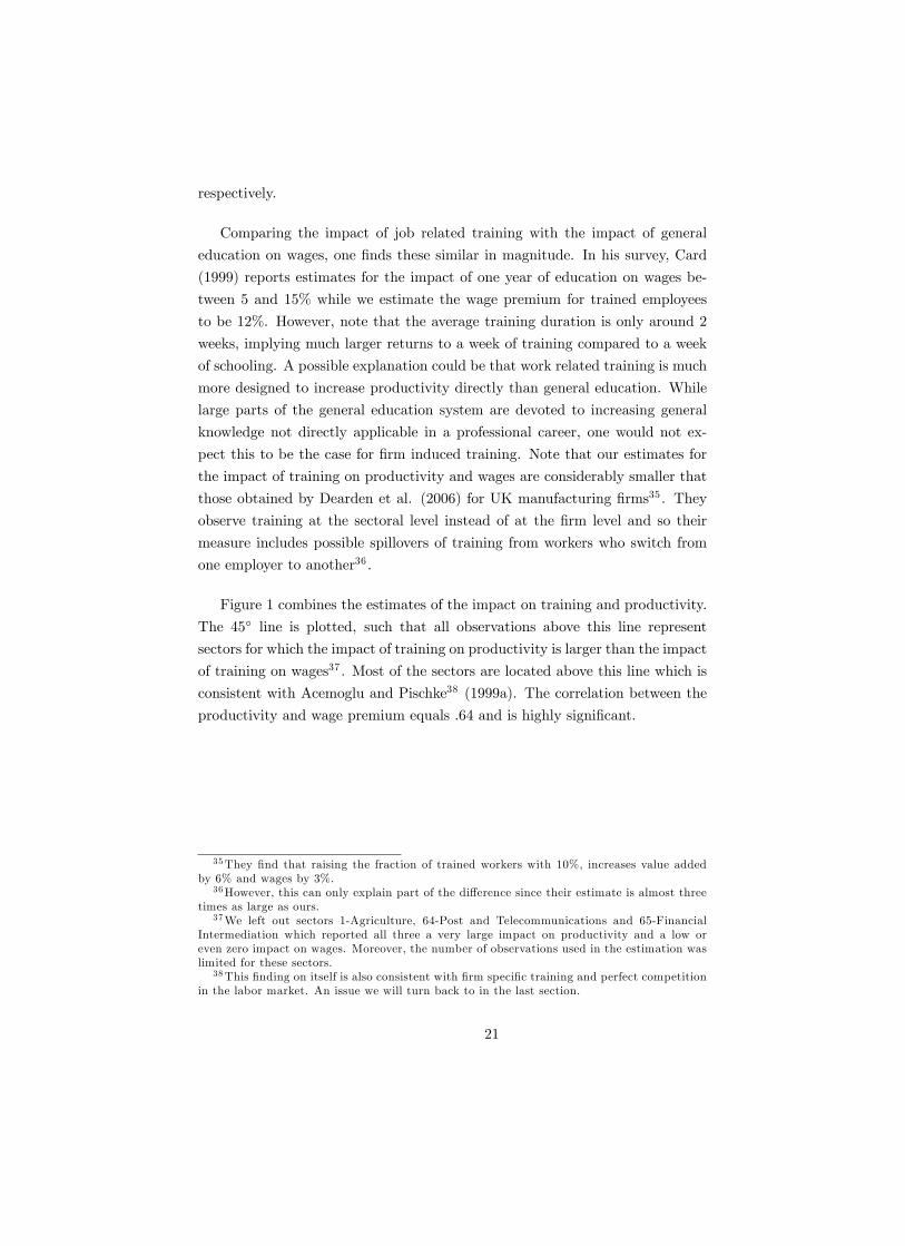
Figure 1 combines the estimates of the impact on training and productivity.

The 45� line is plotted, such that all observations above this line represent

sectors for which the impact of training on productivity is larger than the impact

of training on wages37 . Most of the sectors are located above this line which is

consistent with Acemoglu and Pischke38 (1999a). The correlation between the

productivity and wage premium equals .64 and is highly signi�cant.

35They �nd that raising the fraction of trained workers with 10%, increases value addedby 6% and wages by 3%.

36However, this can only explain part of the di¤erence since their estimate is almost threetimes as large as ours.

37We left out sectors 1-Agriculture, 64-Post and Telecommunications and 65-FinancialIntermediation which reported all three a very large impact on productivity and a low oreven zero impact on wages. Moreover, the number of observations used in the estimation waslimited for these sectors.

38This �nding on itself is also consistent with �rm speci�c training and perfect competitionin the labor market. An issue we will turn back to in the last section.

21

5.3 Training as a continuous variable

In Table 10 we rede�ne the training variable as average training hours per em-

ployee and estimate Equations (10) and (15) to determine the impact of training

intensity on productivity and wages respectively. Again results are reported for

the whole sample and manufacturing and non-manufacturing separate. We con-

trol for the possible endogeneity of training in both the production and wage

equation, applying our estimation strategy described above. The coe¢ cient on

average training intensity in the production function equals :0041 implying that

�T equals :0053 which is considerably higher than our estimate for the impact

of training intensity on wages (:0031). These �gures imply that increasing the

average training hours per employee with 10 hours, raises output by 4% or that a

worker with the average amount of training (40 hours) is around 20% more pro-

ductive than an untrained worker while wages are only around 12% higher. The

di¤erence between the wage and productivity premium is again highly signi�-

cant. Also for the manufacturing and non-manufacturing sectors separately, the

productivity premium is higher than the wage premium, although the di¤erence

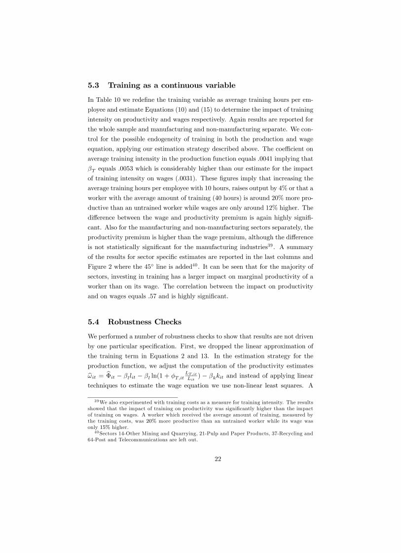
is not statistically signi�cant for the manufacturing industries39 . A summary

of the results for sector speci�c estimates are reported in the last columns and

Figure 2 where the 45� line is added40 . It can be seen that for the majority of

sectors, investing in training has a larger impact on marginal productivity of a

worker than on its wage. The correlation between the impact on productivity

and on wages equals :57 and is highly signi�cant.

5.4 Robustness Checks

We performed a number of robustness checks to show that results are not driven

by one particular speci�cation. First, we dropped the linear approximation of

the training term in Equations 2 and 13. In the estimation strategy for the

production function, we adjust the computation of the productivity estimatesb!it = b�it � �llit � �l ln(1 + �T;it LT;itLit) � �kkit and instead of applying linear

techniques to estimate the wage equation we use non-linear least squares. A

39We also experimented with training costs as a measure for training intensity. The resultsshowed that the impact of training on productivity was signi�cantly higher than the impactof training on wages. A worker which received the average amount of training, measured bythe training costs, was 20% more productive than an untrained worker while its wage wasonly 15% higher.

40Sectors 14-Other Mining and Quarrying, 21-Pulp and Paper Products, 37-Recycling and64-Post and Telecommunications are left out.

22

summary of the results is reported in Table 11. Results are qualitatively and

quantitatively similar to the linear approximation41 , although the magnitude of

the training e¤ect is estimated to be slightly higher. Again, the productivity

premium exceeds the wage premium. Furthermore, we estimate Equations (2)

and (13) with Zellner�s seemingly unrelated regression (SUR) estimator, which

allows the error terms of both equations to be correlated. Again the main re-

sults hold in that the productivity premium is higher than the wage premium

for trained employees42 . The di¤erence is also statistically signi�cant. Third, we

add the average salary in a �rm as control variable in the production function

instead of applying the Ackerberg, Caves and Frazer (2006) estimation strat-

egy. The average �rm-level wage should pick up unobserved labor quality and

productivity di¤erences if workers are paid their marginal product. Also this

strategy leaves our main conclusions una¤ected. Finally, there could be con-

cerns that training intensity does depend on the innovation in productivity. For

example, in case of an unexpected economic downturn �rms could send their

employees more easily on training since the opportunity cost of training is lower

which would create a downward bias in the estimated training coe¢ cient. To

control for this, we alter the moment conditions in Equation (24) and include

training lagged one period instead of contemporaneous training as instrument.

Results are reported in the last two rows of Table 11. Compared to Table 4, the

estimated productivity premium drops somewhat but remains higher than the

wage premium of trained workers.

5.5 Worker heterogeneity

There could be concerns that our methodology does not fully control for worker

heterogeneity and our training coe¢ cient is picking up di¤erences in the mar-

ginal product between di¤erent types of workers unrelated to training. To con-

trol for this, we include in this subsection other forms of worker heterogeneity

in the empirical framework. First, we include measures for the number of blue

collar versus white collar workers and the schooling level of the workforce, but

keep the assumption that these are perfect substitutes to each other. Second,

41Note that the reported coe¢ cients are direct estimates for �T and should be comparedwith �tr=�l in Table 4.

42Here we do not control for the possible endogeneity of training in the production function.For the wage equation, we exclude the control variables. One can argue that the bias ofthe estimated training coe¢ cient is more or less the same in both the wage equation andproduction function .

23

we allow for imperfect substitutability between di¤erent types of workers. The

empirical framework to estimate the productivity and wage premia when the

workforce can be divided among several dimensions is outlined in Appendix A.

Perfect Substitution between Di¤erent Types of Workers

Here, we include di¤erent forms of worker heterogeneity. We maintain however

the assumption that di¤erent types of workers are perfect substitutes. First,

we make a distinction between blue collar workers, white collar workers and

managers. Second, we construct a measure for the education level of the worker

and �nally we include �rm �xed e¤ects which should pick up all other forms of

labor force heterogeneity that are constant over time.

Besides the number of trained employees at each �rm, we also observe the

number of blue collar workers, the number of white collar workers and the num-

ber of managers active in a �rm. We insert the share of blue collars, white collars

and managers in the production function and wage equation (cf. Equations A.5

and A.10)43 and apply again our methodology described above to control for the

endogeneity of training. Again, this leads to conclusions comparable to those in

our base speci�cation. Results for sectors pooled together are reported in Table

12. The coe¢ cient on training drops to :18 in the production function and to

:09 in the wage equation. However, the impact of training remains statistically

signi�cant as well as the di¤erence between the productivity premium and wage

premium. The median of the training coe¢ cient in the production function is

:14 and :11 in the wage equation when estimating the model for each NACE 2

digit sector separately44 .

Moreover, we construct a measure for the average education level of the

workers. Although we do not possess detailed information about the skill com-

position of workers, we observe the education level of every employee that leaves

or enters the �rm in a given year45 . We only observe this information for a lim-

43For the whole sample, around 52% of the workforce is blue-collar, 44% white collar and1.4% management. In the manufacturing sector the shares are respectively 66%, 31% and1.6% and in the services sectors respectively 45%, 51% and 1.3%. The percentages do notsum up to 100% because some of the workers have an unde�ned contract and can not beclassi�ed.

44Dividing the training coe¢ cient by the labor coe¢ cient results in a median productivitypremium of a trained worker of 17%.

45More precise we observe whether the highest education of an entrant or departure isprimary, secundary, higher or university. We de�ne an employee to be high-educated if he

24

ited sample of large �rms46 . Using this data, we compute the educational level

of the in�ow and out�ow of employees and we take the average over all years to

retrieve a proxy for the educational composition of each �rm�s workforce. We

include the share of high-educated employees in both the production function

and wage equation and estimate both equations controlling for the possible en-

dogeneity of inputs (cf. Equations A.7 and A.11) . As can be seen from the

last two rows of Table 12, the training coe¢ cient drops somewhat compared to

the base speci�cation. However, the impact of training on productivity remains

larger than the impact on wages. The results also indicate47 that a schooled

worker is almost two times as productive as an unschooled worker and earns a

substantially higher wage but this wage premium is lower than the productivity

premium, namely 70%.

Finally we repeated the exercise with �rm �xed e¤ects. These should pick up

all unobserved worker heterogeneity that is constant over time. Unfortunately,

using �xed e¤ects to estimate production functions does not perform very well.

When there is measurement error in the input variables, �rst or mean di¤erenc-

ing can exacerbate the bias in the input coe¢ cients estimates. This is especially

true for highly persistent input variables (Griliches and Hausman 1986) such as

capital and training. Results are reported in Appendix C. Table C.1 shows that

for the production function, as expected, unreasonably low estimates of returns

to scale are obtained due to a large decrease in both the capital and labor co-

e¢ cient. Also the training coe¢ cient drops substantially. However, comparing

the impact of training on productivity and wages, we still �nd the productivity

premium for trained employees to be substantially higher than the wage pre-

mium48 and the di¤erence is statistically signi�cant. Estimating training impact

by sector shows that again for the majority of sectors the productivity premium

of trained workers is higher than the wage premium of trained workers as shown

if Figure C.1. The average productivity premium across all sectors equals :10

while the average wage premium is not higher than :026. Again, we suspect

these coe¢ cients to be severely downward biased in contrast to the coe¢ cients

received higher or university education and low-educated if he received at most primary orsecundary education.

46These are �rms that have at least 50 employees, realize a turnover of more than e7:3million or have a total book value of their assets that exceeds e3:65 million.

47These �gures are not reported in the table for expositional reasons.48Although we suspect these estimates to be downward biased, the bias in the production

function should be as large as the bias in the wage equation and thus it still makes sense tocompare both estimates.

25

obtained by applying the Ackerberg, Caves and Frazer (2006) methodology.

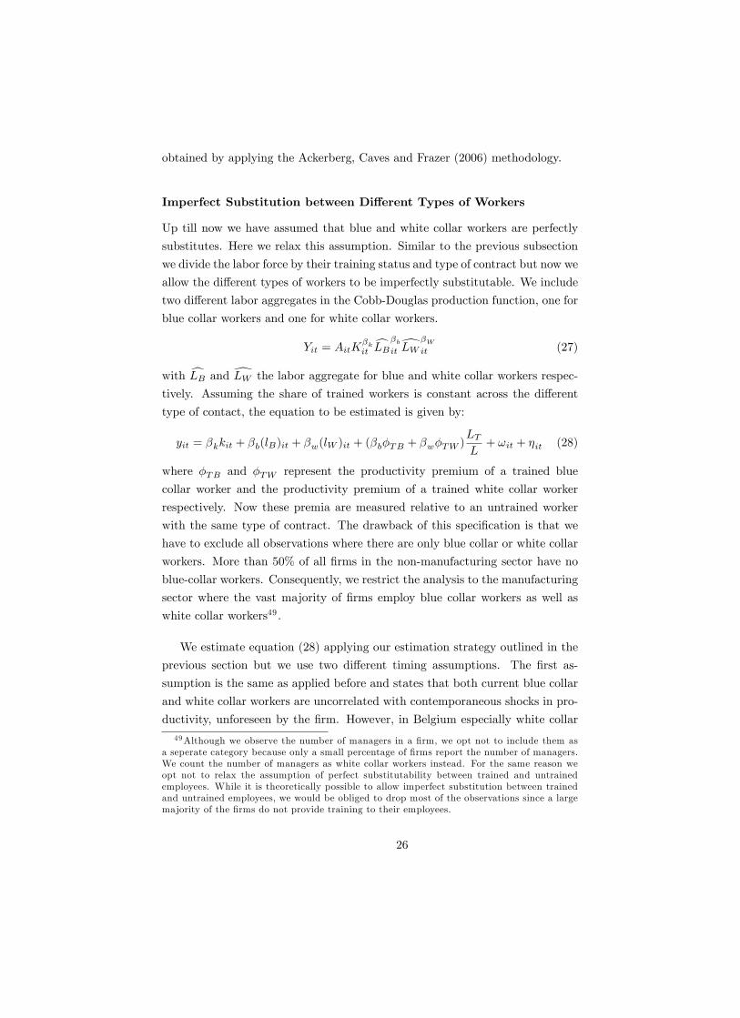
Imperfect Substitution between Di¤erent Types of Workers

Up till now we have assumed that blue and white collar workers are perfectly

substitutes. Here we relax this assumption. Similar to the previous subsection

we divide the labor force by their training status and type of contract but now we

allow the di¤erent types of workers to be imperfectly substitutable. We include

two di¤erent labor aggregates in the Cobb-Douglas production function, one for

blue collar workers and one for white collar workers.

Yit = AitK�kitcLB�bit dLW�W

it (27)

with cLB and dLW the labor aggregate for blue and white collar workers respec-

tively. Assuming the share of trained workers is constant across the di¤erent

type of contact, the equation to be estimated is given by:

yit = �kkit + �b(lB)it + �w(lW )it + (�b�TB + �w�TW )LTL+ !it + �it (28)

where �TB and �TW represent the productivity premium of a trained blue

collar worker and the productivity premium of a trained white collar worker

respectively. Now these premia are measured relative to an untrained worker

with the same type of contract. The drawback of this speci�cation is that we

have to exclude all observations where there are only blue collar or white collar

workers. More than 50% of all �rms in the non-manufacturing sector have no

blue-collar workers. Consequently, we restrict the analysis to the manufacturing

sector where the vast majority of �rms employ blue collar workers as well as

white collar workers49 .

We estimate equation (28) applying our estimation strategy outlined in the

previous section but we use two di¤erent timing assumptions. The �rst as-

sumption is the same as applied before and states that both current blue collar

and white collar workers are uncorrelated with contemporaneous shocks in pro-

ductivity, unforeseen by the �rm. However, in Belgium especially white collar49Although we observe the number of managers in a �rm, we opt not to include them as

a seperate category because only a small percentage of �rms report the number of managers.We count the number of managers as white collar workers instead. For the same reason weopt not to relax the assumption of perfect substitutability between trained and untrainedemployees. While it is theoretically possible to allow imperfect substitution between trainedand untrained employees, we would be obliged to drop most of the observations since a largemajority of the �rms do not provide training to their employees.

26

workers are well protected against dismissal while blue collar workers face less

severe employment protection legislation. Consequently there could be concerns

that blue collar workers are a freely variable input that is adjusted in reaction to

unforeseen productivity shocks. To control for this we also include a speci�cation

where we include blue collar workers lagged one period as instrument instead

of the contemporaneous stock of blue collar workers. Results are reported in

Table 13. ACF1 uses contemporaneous blue collar workers as instrument while

ACF2 uses lagged blue collar workers as instrument. By comparing columns

(1) and (3), one can see that the coe¢ cient on blue collar workers goes down

slightly when blue collar workers are assumed to be a freely variable input. The

coe¢ cient on the share of trained workers is somewhat lower compared to the

speci�cation where we imposed perfect substitution between the di¤erent types

of workers but remains positive and highly signi�cant. If we assume the impact

of training on productivity is the same for blue and white collar workers, the

estimated coe¢ cient implies the productivity premium to be equal to 17% and

18% in the �rst and second speci�cation respectively. Note that the produc-

tivity premium is larger than the wage premium, however the di¤erence is not

signi�cant anymore. We did the same exercise for each NACE 2 digit sector

separately. Results are reported in Table D.1 in the appendix. Not surprisingly,

white collar workers are most important in sectors such as Chemicals, Electrical

Machinery and Medical and Optical Instruments while blue collar workers re-

ceive a high weight in the production function of sectors such as Textiles, Wood

Products and Motor Vehicles. The coe¢ cient on blue collar labor goes down

for the majority of sectors when assuming it is a freely variable input. However,

the coe¢ cient is mostly estimated quite imprecise.

6 Firm speci�c versus general training

In the previous sections, we have established a positive and both statistical and

economic signi�cant impact of training on productivity. Moreover the produc-

tivity premium was found to be larger than the wage premium. Note that this

gap between the productivity and wage premium for trained employees can be

explained equally well by perfect competition and �rm speci�c training as by

imperfect competition and general training. Both explanations however imply

radically di¤erent policy implications. Which of the two theories is the best ex-

planation for our results? Recall that under �rm speci�c training the acquired

27

skills are not applicable in other �rms and the �rm could pay for all train-

ing costs. The �rm recoups all the bene�ts after training through the higher

marginal product of trained workers and equal wages of trained and untrained

workers. Becker (1964) noted that it could be optimal for both workers and

�rms to share bene�ts of training, namely under the form of higher wages but

still lower than the marginal product. Consequently, �rms are less likely to �re

trained workers. Moreover, trained workers are less likely to quit the �rm since

skills are �rm speci�c and they will earn lower wages at other employers. In

general one would expect both dismissal and quit rates to be lower in �rms that

provide a substantial amount of training.

Under imperfect competition in the labor market and general training, a

negative correlation between the dismissal rate and training would arise since

the di¤erence between wage and marginal product is higher for trained workers.

However, when for example the presence of unions is the main source of wage

compression, it is possible that training has no impact on quit rates of workers

since trained workers could earn the same wage at other �rms. To summarize, we

would expect a negative impact of training on the dismissal rate with perfect

competition and speci�c training as well as with imperfect competition and

general training. However, with perfect competition and speci�c training worker

quit rates should be in�uenced by training while this is not necessarily the case

with general training and imperfect competition.

Our dataset allows us not only to compute general separation rates, but also

to distinguish between whether these separations are dismissals initiated by the

�rm or quits initiated by the worker 50 . When we regress the quit and dismissal

rates on the share of trained workers lagged one and two periods, we �nd that

dismissal rates are negatively and signi�cantly a¤ected by the lagged share of

trained employees51 as can be seen from Table E.1 . Quit rates however seem to

be una¤ected by the number of trained workers. The coe¢ cient on the lagged

share of trained employees is not signi�cantly di¤erent from zero52 . The share of

trained employees lagged two periods has even a positive and signi�cant impact

on the quit rates53 . Although not a formal proof, these results suggest that the

training is most likely to be general in nature instead of �rm speci�c. Moreover,

50We only observe these variables for the subset of large �rms.51We control not only for �rm �xed e¤ects but include also in�ows of employees both

contemporaneous and lagged one period and year dummies to control for business cycles.52The p-value is equal to .333.53When aggregating training and seperation rates at the 4 digit level, there was a substan-

tial and signi�cant correlation between the dismissal rate and share of trained employees butnot between the quit rate and share of trained employees.

28

recall that we observe formal training, which is more likely to be general in

nature.

7 Conclusions

This paper empirically investigates the impact of �rm provided training on both

wages and productivity. To this end we make use of a �rm level data set of more

than 170,00 �rms active in Belgium. We are able to measure for each �rm the

amount of employees that received some kind of formal training as well as the

training costs and the hours spent on training for the period 1997 to 2006. The

advantage of using �rm level data compared to individual level data is that we

obtain an objective measure for the productivity of a worker.

After controlling for the possible endogeneity of training we �nd that training

boosts marginal productivity of an employee more than it increases its wage.

More precise, our results indicate that the productivity premium for a trained

employee is on average around 23% while the wage premium is only 12%. We

�nd a slightly higher impact of training in non-manufacturing compared to

manufacturing sectors. Our results are robust across di¤erent speci�cations

and de�nitions of the training variable. When controlling for other sources

of worker heterogeneity, our estimates for the productivity and wage premium

drop to 17% and 11% respectively and the di¤erence between the two premia

remains substantial and statistically signi�cant. Also relaxing the assumption

of perfect substitutability between di¤erent types of workers leaves our main

�ndings una¤ected. There exists considerable sector heterogeneity in the impact

of training on both productivity and wages. Sectors with the largest e¤ects of

training include the Chemical sector and Rubber and Plastic sector.

Our results are consistent with recent theories such as Acemoglu and Pischke

(1999a) that explain �rm provided general training by imperfect competition in

the labor market and wage compression. This �nding can have important pol-

icy implications. The standard result of Becker (1964) is that if workers are

not credit constrained, training investments are e¢ cient and as such, govern-

ment intervention is unnecessary or should be directed to the credit markets.

However, with imperfect labor markets and a compressed wage structure, there

could be underinvestment in training from a social point of view. For example,

when making their training decisions, �rms do not take into account the possi-

ble externalities for future employers of trained workers (Acemoglu and Pischke

29

1999b). This opens possibilities for the government to implement training sub-

sidies. However, an assessment of the optimal versus the current amount of

training and the extent of government intervention to reach this optimal level

lies outside the scope of this paper. We leave this for future research.

30

8 References

Acemoglu, D., & Pischke, J.-S. (1998). Why Do Firms Train? Theory andEvidence. Quarterly Journal of Economics, 113(1), 79-119.

Acemoglu, D. and J.S. Pischke (1999a). "The Structure of Wages and Invest-ment in General Training." Journal of Political Economy 107(3): 539-572.

Acemoglu, D. and J.S. Pischke (1999b). "Beyond Becker: Training in ImperfectLabour Markets." The Economic Journal 109(Feb.): 112-142.

Ackerberg, D., Benkard, L., Berry, S., and Pakes, A. (2005) �Econometric Toolsfor Analyzing Market Outcomes�, Forthcoming chapter in Handbook of Econo-metrics, Volume 6

Ackerberg D., K. Caves and G. Frazer (2006). "Structural Identi�cation ofProduction Functions", mimeo.

Bartel, A. P. (1995). "Training, Wage Growth, and Job Performance: Evidencefrom a Company Database." Journal of Labor Economics 13(3): 401-425.

Becker, G.S. (1964). Human Capital. Chicago: The University of Chicago Press.

Black, S. E. and L. M. Lynch (1996). "Human-Capital Investments and Pro-ductivity." The American Economic Review 86(2): 263-267.

Black, S. E. and L. M. Lynch (2001). "How To Compete: The Impact Of Work-place Practices And Information Technology On Productivity." The Review ofEconomics and Statistics 83(3): 434-445.

Blundell, R. and S. Bond (1998). "Initial conditions and moment restrictionsin dynamic panel data models." Journal of Econometrics 87(1): 115-143.

Blundell, R., Dearden, L., Meghir, C., & Sianesi, B. (1999). Human capitalinvestment: the returns from education and training to the individual, the �rmand the economy. Fiscal Studies, 20(1): 1-23.

Bond, S. and M. W. Söderbom (2005). Adjustment costs and the identi�cationof Cobb Douglas production functions, Institute for Fiscal Studies.

Booth, A. L. (1991). "Job-Related Training: Who Receives it and What Is itWorth? ." Oxford Bulletin of Economics & Statistics 53(3): 281-294.

Card, D. (1999). The causal e¤ect of education on earnings. Handbook of LaborEconomics. O. Ashenfelter and D. Card, Elsevier. Volume 3, Part 1: 1801-1863.

Dearden, L., Reed, H., & Reenen, J. V. (2006). "The Impact of Training onProductivity and Wages: Evidence from British Panel Data." Oxford Bulletinof Economics and Statistics 68(4): 397-421.

31

De Loecker, J. (2007). "Product Di¤erentiation, Multi-product Firms and Es-timating the Impact of Trade Liberalization on Productivity." National Bureauof Economic Research Working Paper Series No. 13155.

European Commission (2007) "Strengthening Continuing Vocational Trainingat the Initiative of the Enterprise." Employment in Europe 2007, O¢ ce foro¢ cial publications of the European Communities, Luxembourg.

Frazer G. (2001) "Linking Firms and Workers: Heterogeneous Labor and Re-turns to Education." mimeo Yale University

Griliches and Hausman (1986) "Errors in Variables in Panel Data", Journal ofEconometrics, 31(1), pp. 93-118.

Hellerstein, J. K. and D. Neumark (1999). "Sex, wages, and productivity: Anempirical analysis of Israeli �rm-level data." International Economic Review40(1): 95.

Hellerstein, J. K., D. Neumark, and K. R. Troske. (1999). "Wages, Productivity,and Worker Characteristics: Evidence from Plant Level Production Functionsand Wage Equations." Journal of Labor Economics 17(3): 409-446.

Holzer, H. J., R. N. Block, M. Cheatham, and J.H. Knott (1993). "Are trainingsubsidies for �rms e¤ective? The Michigan experience." Industrial & LaborRelations Review 46(4): 625-636.

Jones, P. (2001). "Are educated workers really more productive?" Journal ofDevelopment Economics 64(1): 57-79.

Lucas, R. E. (1988). "On the mechanics of economic development." Journal ofMonetary Economics 22(1): 3-42.

Levinsohn, J. and A. Petrin (2003). "Estimating Production Functions UsingInputs to Control for Unobservables." Review of Economic Studies 70(243):317-341.

Mincer, J., (1974). Schooling, Experience, and Earnings, Colombia Univ. Press,New York

Moretti, E. (2004). "Workers� Education, Spillovers, and Productivity: Ev-idence from Plant-Level Production Functions." American Economic Review94(3): 656-690

Olley, G. S. and A. Pakes (1996). "The Dynamics of Productivity in theTelecommunications Equipment Industry." Econometrica 64(6): 1263-1297.

OECD (2007). "OECD Economic Surveys: Belgium", Paris.

Van Biesebroeck, J. (2007). "Wages Equal Productivity. Fact or Fiction?".Working Paper University of Toronto, Department of Economics.

32

9 Tables

Table 1: Summary StatisticsTotal Training No Training

Employment 16.9 84.8 6.67Turnover (�1000e) 10,078 37,245 2,820Labor Cost per Worker (�1000e) 35.1 44.8 33.7Labor Productivity (�1000e) 63.9 73.0 62.5Capital/Labor (�1000e) 75.5 69.8 76.3Observations 919,077 54,867 864,210Nr. Firms 171,210 15,499 155,711Proportion of Trained Workers 0.53Cost of Training per Worker Trained 1,581Hours Training per Worker Trained 39.8

Table 2: Summary RegressionsDependent Var. (1) (2) (3) # Obs

Employment (ln) 2.27* 1.97* 919,077Turnover (ln) 2.56* 0.31* 0.26* 380,091Lab. Costs (ln) 0.36* 0.27* 0.18* 919,077Lab. Prod. (ln) 0.24* 0.40* 0.27* 910,615Capital/Labor (ln) -0.27* 0.35* 0.27* 891,984

* Denotes sigini�cant at 1 perc. level.(1) Regression of dependent variable on training dummy,(2) Similar to (1) but controlling for size (employment),(3) Similar to (2) but with NACE 4 digit dummies.

33

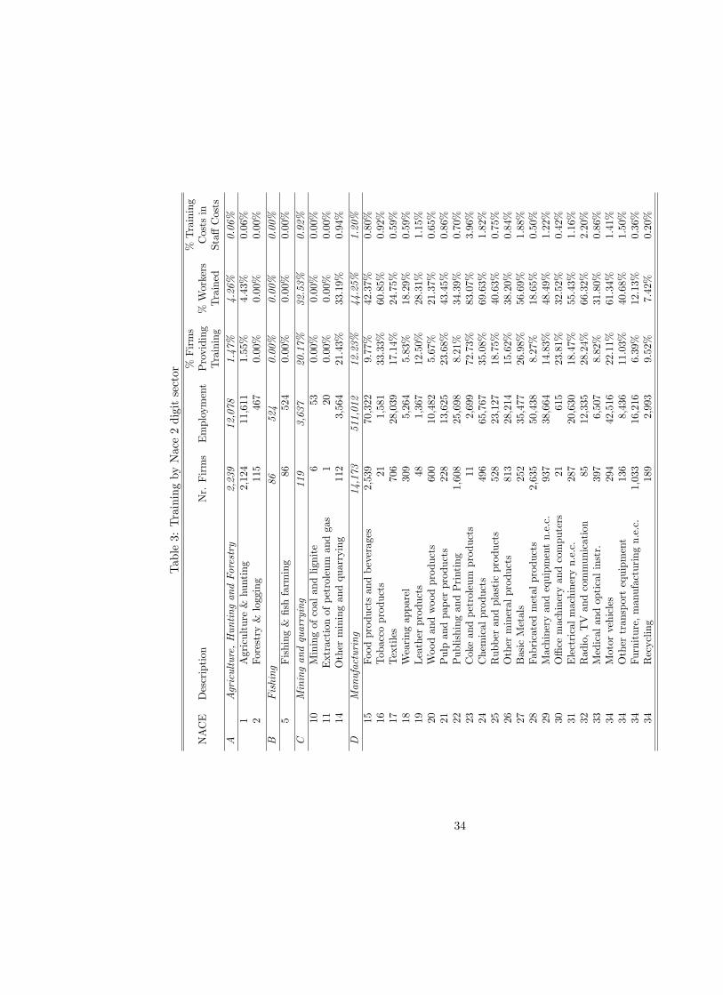
Table3:TrainingbyNace2digitsector%Firms

%Training

NACE

Description

Nr.Firms

Employment

Providing

%Workers

Costsin

Training

Trained

Sta¤Costs

AAgriculture,HuntingandForestry

2,239

12,078

1.47%

4.26%

0.06%

1Agriculture&hunting

2,124

11,611

1.55%

4.43%

0.06%

2Forestry&logging

115

467

0.00%

0.00%

0.00%

BFishing

86524

0.00%

0.00%

0.00%

5Fishing&�shfarming

86524

0.00%

0.00%

0.00%

CMiningandquarrying

119

3,637

20.17%

32.53%

0.92%

10Miningofcoalandlignite

653

0.00%

0.00%

0.00%

11Extractionofpetroleum

andgas

120

0.00%

0.00%

0.00%

14Otherminingandquarrying

112

3,564

21.43%

33.19%

0.94%

DManufacturing

14,173

511,012

12.23%

44.25%

1.20%

15Foodproductsandbeverages

2,539

70,322

9.77%

42.37%

0.80%

16Tobaccoproducts

211,581

33.33%

60.85%

0.92%

17Textiles

706

28,039

17.14%

24.75%

0.59%

18Wearingapparel

309

5,264

5.83%

18.29%

0.59%

19Leatherproducts

481,367

12.50%

28.31%

1.15%

20Woodandwoodproducts

600

10,482

5.67%

21.37%

0.65%

21Pulpandpaperproducts

228

13,625

23.68%

43.45%

0.86%

22PublishingandPrinting

1,608

25,698

8.21%

34.39%

0.70%

23Cokeandpetroleum

products

112,699

72.73%

83.07%

3.96%

24Chemicalproducts

496

65,767

35.08%

69.63%

1.82%

25Rubberandplasticproducts

528

23,127

18.75%

40.63%

0.75%

26Othermineralproducts

813

28,214

15.62%

38.20%

0.84%

27BasicMetals

252

35,477

26.98%

56.69%

1.88%

28Fabricatedmetalproducts

2,635

50,438

8.27%

18.65%

0.50%

29Machineryandequipmentn.e.c.

937

38,664

14.83%

48.49%

1.22%

30O¢cemachineryandcomputers

21615

23.81%

32.52%

0.42%

31Electricalmachineryn.e.c.

287

20,630

18.47%

55.43%

1.16%

32Radio,TVandcommunication

8512,335

28.24%

66.32%

2.20%

33Medicalandopticalinstr.

397

6,507

8.82%

31.80%

0.86%

34Motorvehicles

294

42,516

22.11%

61.34%

1.41%

34Othertransportequipment

136

8,436

11.03%

40.68%

1.50%

34Furniture,manufacturingn.e.c.

1,033

16,216

6.39%

12.13%

0.36%

34Recycling

189

2,993

9.52%

7.42%

0.20%

34

%Firms

%Training

NACE

Description

Nr.Firms

Employment

Providing

%Workers

Costsin

Training

Trained

Sta¤Costs

EElectricity,gasandwatersupply

5322,559

45.28%

78.83%

2.42%

40Electricity,gasandhotwater

3017,248

46.67%

81.55%

2.68%

41Collectionandwaterdistribution

235,311

43.48%

70.01%

0.98%

FConstruction

17,079

175,432

2.82%

9.69%

0.20%

45Construction

17,079

175,432

2.82%

9.69%

0.20%

GWholesaleandretailtrade

36,150

374,016

3.93%

27.47%

0.70%

50Saleandrepairmotorvehicles

5,746

50,986

5.55%

17.03%

1.03%

51Wholesaletrade

14,166

162,870

6.01%

21.32%

0.52%

52Retailtrade

16,238

160,160

1.55%

37.04%

0.85%

HHotelsandrestaurants

9,084

54,837

0.72%

16.69%

0.21%

55Hotelsandrestaurants

9,084

54,837

0.72%

16.69%

0.21%

ITransport,storageandcommunication

6,598

187,649

6.96%

37.52%

1.42%

60LandTransport;pipelines

4,205

78,416

4.19%

17.18%

0.48%

61Watertransport

96939

7.29%

11.61%

0.23%

62Airtransport

294,687

20.69%

33.07%

1.87%

63Supportingtransportactivities

1,839

44,674

12.72%

31.33%

1.16%

64Postandtelecommunications

429

58,933

8.39%

70.06%

2.71%

JFinancialintermediation

4,240

24,642

2.88%

28.39%

1.50%

60Financialintermediation

1,650

12,150

2.97%

30.22%

2.18%

60Insuranceandpensionfunding

23192

8.70%

5.73%

0.07%

60Auxiliary�nancialactivities

2,567

12,300

2.77%

26.93%

0.81%

KRealestate,renting,businessactivities

19,699

326,061

6.67%

18.84%

0.79%

60Realestateactivities

2,970

13,586

3.70%

8.16%

0.15%

60Rentingactivities

658

4,815

4.41%

9.49%

0.22%

60Computerandrelatedactivities

2,431

37,417

10.51%

38.49%

1.45%

60Researchanddevelopment

822,993

17.07%

55.46%

1.45%

60Otherbusinessactivities

13,558

267,250

6.67%

16.39%

0.68%

TOTAL(SERVICESANDMANUFACTURING)

109,520

1,692,447

5.19%

30.33%

0.96%

35

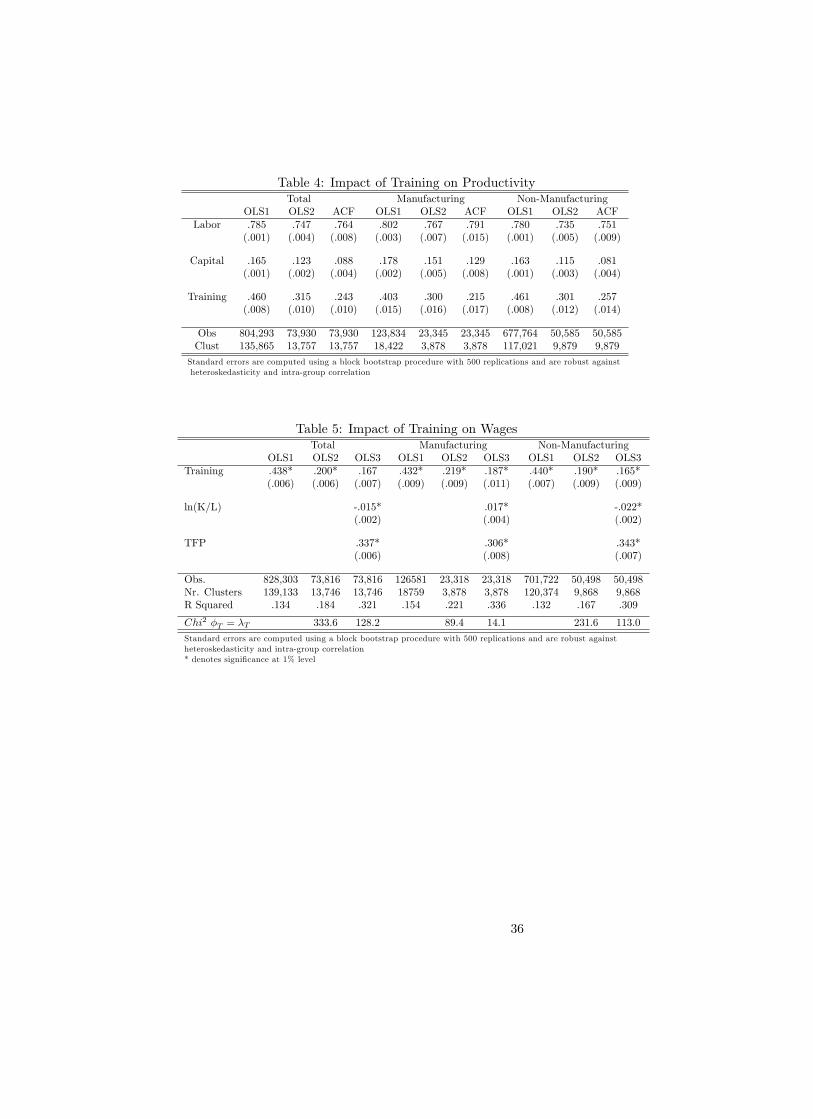
Table 4: Impact of Training on ProductivityTotal Manufacturing Non-Manufacturing

OLS1 OLS2 ACF OLS1 OLS2 ACF OLS1 OLS2 ACFLabor .785 .747 .764 .802 .767 .791 .780 .735 .751

(.001) (.004) (.008) (.003) (.007) (.015) (.001) (.005) (.009)

Capital .165 .123 .088 .178 .151 .129 .163 .115 .081(.001) (.002) (.004) (.002) (.005) (.008) (.001) (.003) (.004)

Training .460 .315 .243 .403 .300 .215 .461 .301 .257(.008) (.010) (.010) (.015) (.016) (.017) (.008) (.012) (.014)

Obs 804,293 73,930 73,930 123,834 23,345 23,345 677,764 50,585 50,585Clust 135,865 13,757 13,757 18,422 3,878 3,878 117,021 9,879 9,879

Standard errors are computed using a block bootstrap procedure with 500 replications and are robust againstheteroskedasticity and intra-group correlation

Table 5: Impact of Training on WagesTotal Manufacturing Non-Manufacturing

OLS1 OLS2 OLS3 OLS1 OLS2 OLS3 OLS1 OLS2 OLS3Training .438* .200* .167 .432* .219* .187* .440* .190* .165*

(.006) (.006) (.007) (.009) (.009) (.011) (.007) (.009) (.009)

ln(K/L) -.015* .017* -.022*(.002) (.004) (.002)

TFP .337* .306* .343*(.006) (.008) (.007)

Obs. 828,303 73,816 73,816 126581 23,318 23,318 701,722 50,498 50,498Nr. Clusters 139,133 13,746 13,746 18759 3,878 3,878 120,374 9,868 9,868R Squared .134 .184 .321 .154 .221 .336 .132 .167 .309

Chi2 �T = �T 333.6 128.2 89.4 14.1 231.6 113.0

Standard errors are computed using a block bootstrap procedure with 500 replications and are robust againstheteroskedasticity and intra-group correlation* denotes signi�cance at 1% level

36

Table 6: Results Productivity Manufacturing SectorsLabor Capital Training Nr. Obs

OLS ACF OLS ACF OLS ACF Obs Clust

15 Food Products .789 .729 .175 .174 .165 .130 3,571 600(.018) (.035) (.016) (.036) (.031) (.034)

17 Textile Products .753 .720 .154 .133 .319 .227 1,729 298(.027) (.094) (.018) (.038) (.042) (.047)

18 Wearing Apparel .665 .675 .227 .160 .101 .049 364 66(.112) (.240) (.040) (.094) (.193) (.124)

20 Wood Products .668 .700 .142 .102 .659 .264 588 110(.038) (.266) (.034) (.074) (.135) (.106)

21 Paper Products .853 .658 .120 .269 .149 .036 685 98(.060) (.179) (.035) (.099) (.070) (.057)

22 Publishing .804 .828 .103 .077 .154 .157 1,764 319(.027) (.071) (.017) (.023) (.064) (.049)

24 Chemical Products .841 .816 .125 .116 .405 .305 2,134 331(.029) (.067) (.026) (.047) (.063) (.053)

25 Rubber and Plastic .788 .803 .183 .172 .341 .255 1,477 227(.030) (.228) (.022) (.064) (.047) (.050)

26 Mineral Products .798 .773 .135 .157 .219 .174 1,917 311(.023) (.065) (.020) (.047) (.048) (.043)

27 Basic Metals .802 .772 .171 .191 .105 .084 995 146(.034) (.112) (.025) (.049) (.068) (.060)

28 Metal Products .760 .733 .139 .129 .176 .102 2,779 478(.020) (.033) (.012) (.016) (.038) (.039)

29 Machinery .822 .789 .114 .134 .287 .197 1,681 283(.034) (.076) (.021) (.029) (.051) (.051)

31 Electrical Machinery .800 .745 .143 .132 .236 .219 665 104(.038) (.086) (.027) (.059) (.091) (.102)

32 Radio, TV and Telecom .905 .894 .068 .064 .204 .151 302 54(.075) (.144) (.071) (.102) (.108) (.144)

33 Medical Eq., Optical Instr. .813 .791 .047 .012 .256 .182 346 64(.074) (.147) (.054) (.080) (.101) (.131)

34 Motor Vehicles .843 .776 .108 .120 .050 .087 752 121(.022) (.042) (.020) (.027) (.068) (.061)

36 Furniture, Manuf. n.e.c. .667 .551 .184 .167 .087 .137 1,101 181(.039) (.086) (.025) (.055) (.057) (.063)

Standard errors are computed using a block bootstrap procedure with 500 replications and are robustagainst heteroskedasticity and intra-group correlation

37

Table 7: Results Productivity Non-Manufacturing SectorsLabor Capital Training Obs.

OLS ACF OLS ACF OLS ACF Obs. Clust.

1 Agriculture .701 .648 .097 .132 .196 .339 459 96(.058) (.077) (.035) (.074) (.164) (.134)

14 Mining .837 .798 .198 .267 .324 .017 345 60(.059) (.250) (.056) (.305) (.120) (.143)

37 Recycling .737 .737 .164 .124 .239 .242 364 79(.071) (.108) (.032) (.067) (.135) (.194)

45 Construction .774 .773 .136 .134 .184 .123 5,521 939(.016) (.038) (.010) (.017) (.022) (.023)

50 Sales Motor Vehicles .804 .803 .091 .081 .295 .179 3,974 746(.019) (.052) (.013) (.026) (.042) (.033)

51 Wholesale Trade .742 .758 .077 .061 .351 .317 21,380 4,017(.008) (.013) (.005) (.006) (.021) (.022)

52 Retail Trade .779 .735 .158 .158 .125 .135 4,104 869(.017) (.054) (.012) (.029) (.030) (.040)

55 Hotels and Restaurants .820 .798 .123 .124 .107 .084 877 164(.030) (.058) (.022) (.047) (.043) (.047)

60 Land Transport .753 .726 .144 .147 .116 .079 2,617 455(.021) (.070) (.015) (.043) (.060) (.043)

63 Transport Activities .633 .681 .174 .133 .305 .222 1,892 411(.023) (.029) (.015) (.022) (.052) (.051)

64 Post and Telecommunications .753 .749 .202 .175 .283 .284 337 86(.049) (.120) (.031) (.058) (.175) (.161)

65 Financial Intermediation .778 .766 .180 .214 .560 .453 315 79(.072) (.189) (.048) (.123) (.264) (.209)

70 Real Estate .551 .523 .154 .090 .352 .252 1,360 275(.028) (.048) (.020) (.040) (.091) (.114)

71 Renting of Machinery .507 .575 .367 .300 .104 .149 487 96(.050) (.127) (.051) (.060) (.125) (.090)

72 Computer and Related Activities .855 .849 .084 .088 -.030 .002 1,587 393(.020) (.026) (.010) (.014) (.039) (.046)

74 Other Business Activities .777 .774 .109 .093 .196 .201 4,313 975(.014) (.028) (.009) (.015) (.031) (.038)

Standard errors are computed using a block bootstrap procedure with 500 replications and are robustagainst heteroskedasticity and intra-group correlation

38

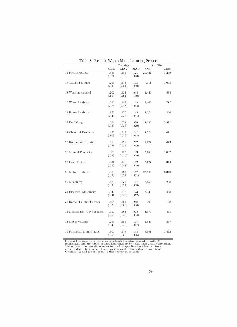
Table 8: Results Wages Manufacturing SectorsTraining Nr. Obs.

OLS1 OLS2 OLS3 Obs. Clust

15 Food Products .353 .155 .121 21,447 3,259(.021) (.019) (.023)

17 Textile Products .296 .171 .118 7,311 1,068(.030) (.031) (.040)

18 Wearing Apparel .702 .123 .044 3,446 535(.190) (.224) (.189)

20 Wood Products .290 .185 .112 5,466 787(.073) (.048) (.054)

21 Paper Products .372 .179 .142 2,274 300(.044) (.036) (.041)

22 Publishing .364 .074 .078 14,398 2,322(.030) (.026) (.029)

24 Chemical Products .455 .312 .242 4,774 671(.103) (.032) (.043)

25 Rubber and Plastic .413 .239 .212 5,027 673(.031) (.025) (.042)

26 Mineral Products .306 .155 .143 7,680 1,062(.028) (.025) (.028)

27 Basic Metals .331 .146 .112 2,627 344(.053) (.048) (.048)

28 Metal Products .309 .195 .157 22,864 3,340(.020) (.031) (.031)

29 Machinery .429 .237 .197 8,253 1,228(.033) (.031) (.038)

31 Electrical Machinery .342 .218 .173 2,743 408(.041) (.049) (.057)

32 Radio, TV and Telecom .405 .287 .248 799 128(.078) (.059) (.080)

33 Medical Eq., Optical Instr. .359 .104 .073 3,079 475(.058) (.045) (.054)

34 Motor Vehicles .264 .123 .107 2,536 367(.046) (.045) (.047)

36 Furniture, Manuf. n.e.c. .305 .177 .143 9,591 1,442(.058) (.050) (.056)

Standard errors are computed using a block bootstrap procedure with 500replications and are robust against heteroskedasticity and intra-group correlation.The number of observations refers to the �rst speci�cation where all �rmsare included. The number of observations used in the restricted sample ofColumns (2) and (3) are equal to those reported in Table 7

39

Table 9: Results Wages Non-Manufacturing SectorsTraining Nr. Obs

OLS1 OLS2 OLS3 Obs. Clust

1 Agriculture .428 .125 .145 14,077 2,424(.058) (.090) (.074)

14 Mining .329 .091 .050 1,126 157(.083) (.069) (.073)

37 Recycling .305 .267 .254 1,668 274(.074) (.096) (.095)

45 Construction .335 .150 .134 133,695 21,316(.014) (.018) (.019)

50 Sales Motor Vehicles .375 .185 .137 48,134 7,519(.021) (.024) (.027)

51 Wholesale Trade .468 .191 .181 120,834 19,621(.014) (.013) (.014)

52 Retail Trade .254 .078 .060 110,918 19,138(.020) (.020) (.025)

55 Hotels and Restaurants .326 .122 .104 54,774 10,545(.032) (.031) (.034)

60 Land Transport .195 .094 .061 35,808 5,451(.022) (.029) (.028)

63 Transport Activities .175 .121 .100 14,923 2,450(.026) (.032) (.034)

64 Post and Telecommunications .409 -.014 -.082 2,869 650(.067) (.105) (.106)

65 Financial Intermediation .401 .025 -.021 10,220 1,928(.052) (.107) (.115)

70 Real Estate .542 .303 .265 20,425 4,013(.042) (.064) (.072)

71 Renting of Machinery .547 .129 .084 4,971 905(.040) (.059) (.051)

72 Computer and Related Activities .316 -.024 -.005 15,837 3,281(.021) (.031) (.037)

74 Other Business Activities .409 .143 .137 90,400 17,081(.012) (.021) (.024)

Standard errors are computed using a block bootstrap procedure with 500replications and are robust against heteroskedasticity and intra-group correlation.The number of observations refers to the �rst speci�cation where all �rms areincluded. The number of observations used in the restricted sample of Columns(2) and (3) are equal to those reported in Table 7

40

Table 10: Training as Average Training Hours per WorkerTotal Manufacturing Non-Manufacturing Each Sector Seperat.

Prod. Wage Prod. Wage Prod. Wage.Capital .090 .133 .082 �T

(.004) (.010) (.004) Min -.0003Labor .774 .798 .759 Max .0134

(.007) (.032) (.009) Av. .0044Training .0041 .0031 .0032 .0032 .0047 .0032

(.0002 (.0001 (.0003) (.0002) (.0003) (.0002) �TTFP .343 .314 .349 Min .0003

(.005) (.015) (.007) Max .0079Cap/Lab -.014 .018 -.022 Av. .0024

(.002) (.004) (.002)Test for �T = �TChi2 71.7 3.19 84.9p� value .00 .07 .00

Standard errors are computed using a block bootstrap procedure with 500 replications andare robust against heteroskedasticity and intra-group correlation

Table 11: Results Further Robustness ChecksTotal Manufacturing Non-Manufacturing

Prod. Wage Prod. Wage Prod. WageNon-Linear Speci�cation .374 .233 .313 .259 .407 .239

SUR Model .295 .208 .310 .225 .273 .199(.006) (.005) (.009) (.007) (.008) (.006)

Wage as Control .189 .168 .201 .178 .171 .160(.010) (.006) (.018) (.009) (.013) (.008)

Lagged Training .173 .147 .145 .168 .171 .138(.011) (.007) (.016) (.012) (.015) (.010)

Standard errors are computed using a block bootstrap procedure with 500replications and are robust against heteroskedasticity and intra-group correlation

Table 12: Worker Heterogeneity, Perfect SubstitutionTotal Manufacturing Non-Manufacturing

Prod. Wage Prod. Wage Prod. Wage.Type of Contract (�l�T or �T ) .176 .141 .173 .174 .180 .122

(.010) (.006) (.015) (.008) (.013) (.008)

Schooling (�l�T or �T ) .152 .090 .155 .128 .149 .076(.010) (.009) (.015) (.010) (.013) (.008)

Productivity estimates refer to estimation of Equations (A.5) and (A.7) and arecontrolled for simultaneity bias (ACF procedure).Wage results refer to estimationof Equations (A.10) and (A.11) by ordinary least squares with added control variables.Standard errors are computed using a block bootstrap procedure 500 replicationsand are robust against heteroskedasticity and intra-group correlation

41

Table 13: Blue versus White Collar Workers, Imperfect SubstitutionACF1 ACF2

Prod. Wage Prod. WageCapital .123 .124

(.006) (.006)Blue Collar .360 .338

(.020) (.030)White Collar .439 .448

(.016) (.018)Training .136 .155 .138 .152

(.015) (.009) (.015) (.009)TFP .180 .182

(.008) (.008)Cap/Lab .029 .029

(.003) (.003)

Nr. Obs. 19,679 19,679Nr. Clust. 3,414 3,414

Test for �T = �TChi2 .59 1.12p� value .44 .29

Results ACF method with contemporaneous blue collarworkers (ACF1) and blue collar workers lagged oneperiod as instruments.Standard errors are computed using a block bootstrapprocedure with 500 replications and are robust againstheteroskedasticity and intra-group correlation

42

Figure 1: Impact Training on Productivity and Wages

74

72

71

70

63

60 55

52

51

50

45

37

36

34

33

32

31

29

2827

26

25

24

22

21

20

18

17

15

14

0.1

.2.3

.4.5

Impa

ct o

n P

rodu

ctiv

ity

0 .1 .2 .3 .4 .5Impact on Wages

Productivity: ACF; Wages: OLS with Control Variables

Impact Training on Wages and Productivity

43

Figure 2: Impact Training on Productivity and Wages; Training as Hours Train-ing per Worker.

74

72

71

70

65

63

60 5552

51

50

4536

34

33

32

3129

28

2726

25

24

22

20

18

17

15

1

0.0

02.0

04.0

06.0

08.0

1.0

12.0

14Im

pact

 on 

Pro

duct

ivity

0 .002 .004 .006 .008 .01 .012 .014Impact on Wages

Productivity: ACF; Wages: OLS with Control Variables

Training as Continuous VariableImpact Training on Wages and Productivity

44

Appendix

A Other sources of worker heterogeneity

A.1 ProductivityThe derivations in the main text assumed that training is the only source ofheterogeneity in the labor force. This appendix shows how we can generalizethe expression for the labor aggregate when workers can be di¤erentiated bymultiple characteristics. Next to training we also observe whether the workersare blue collar, white collar or part of the management sta¤ and their schoolinglevel. When there are multiple observed characteristics, the workforce can bedescribed by all K possible combinations of these characteristics and the laboraggregate bL can be written as:

bL = L0 + K�1Xk=1

(1 + �k)Lk (A.1)

where again �k is the productivity premium of a type k worker relative toa worker of the base type (�k =

MPk�MP0MP0

). When we include for exampletraining and the type of contract (blue collar, white collar or management) asworker characteristics, there are six di¤erent types of workers namely untrainedblue collar, untrained white collar, untrained management, trained blue collar,trained white collar and trained management. If the base type is an untrainedblue collar worker, then for example the relative productivity premium of atrained white collar worker, �TW , is de�ned as �TW = MPTW�MPUB

MPUBwith

MPTW the marginal product of a trained white collar worker and MPUB themarginal product of an untrained blue collar worker. Again, the labor aggregatecan be rewritten as: bL = L 1 + K�1X

k=1

�kLkL

!(A.2)

or rewriting the productivity premium of a trained white collar worker, �TW asthe product of productivity premia of white collars �W , trained workers �T andan interaction term54 �T�W , �TW =

�(1 + �W )(1 + �T )(1 + �T�W )� 1

�and

the productivity premium of a trained manager as the product of productivitypremia of managers �Z , trained workers and an interaction term �T�Z , �TZ =�(1 + �Z)(1 + �T )(1 + �T�Z)� 1

�. When the interaction term for trained white

collars is larger than zero, training of white collar workers pays o¤ more thantraining of blue collar workers and the other way around when the interaction isnegative. A value of zero for this parameter means that marginal productivityincreases by the same amount for white collar workers as for blue collar workersin response to training. A similar reasoning applies for the interaction term of

54To be precise, �T represents the productivity premium of a trained blue collar workercompared to an untrained blue collar worker. Likewise, �W is the productivity premium ofan untrained white collar worker compared to an untrained blue collar worker.

45

trained managers. The labor aggregate can be written as:

bL = L

�1 + �Z

LUZL

+ �WLUWL

+ �TLTBL

+�(1 + �Z)(1 + �T )(1 + �Z�T )� 1

� LTZL

+�(1 + �W )(1 + �T )(1 + �W�T )� 1

� LTWL

�(A.3)

Note that to estimate the productivity premium of each di¤erent type of worker,we need to observe the proportion of each type in the total workforce. Unfortu-nately we do not observe the number of trained and untrained workers for eachemployee type. This forces us to make some simplifying assumptions similar toother studies that divide the labor force among several dimensions (e.g. VanBiesebroeck, 2007). First, we have to assume that he relative di¤erences in mar-ginal productivity between two workers that di¤er by one characteristic are thesame irrespective of what their other characteristics are. This means that therelative marginal product of trained workers compared to untrained workers isthe same for all di¤erent types of workers and consequently �Z�T = �W�T = 0.Furthermore we restrict the proportion of one type of workers to be constantacross other groups de�ned by the other characteristics or LTZ

LZ= LTW

LW= LT

L .Applying these restrictions to equation A.3 gives

bL = L�(1 + �Z LZL + �WLWL)(1 + �T

LTL)

�(A.4)

The expression for the production function that is taken to the data is thefollowing:

y = �0 + �kk + �ll + �l�TLTL+ �l�W

LWL+ �l�Z

LZL+ � (A.5)

Next to a speci�cation where we make distinction between the type of con-tracts, we moreover divide the labor force among the schooling level and trainingstatus of the workers. Schooling is constructed such that the variable takes ontwo values, namely high-schooled and low-schooled. The restricted version ofthe labor aggregate can be written as

bL = L(1 + �S LSL )(1 + �T LTL ) (A.6)

where LS is the number of high schooled workers and �S represents the pro-ductivity premium of a high-schooled worker relative to a low-schooled worker.The expression for the production function becomes:

y = �0 + �kk + �ll + �l�TLTL+ �l�S

LSL+ � (A.7)

46

A.2 WagesIn a similar way, we can extend the empirical framework for estimating wagepremia by including multiple characteristics of the workforce. Imposing similarrestrictions as for estimating the productivity premium, namely equal propor-tions and equal relative wage premia, we can write the average wage in a �rmas

W =WBU (1 + �ZLZL+ �W

LWL)(1 + �T

LTL) (A.8)

where WBU is the wage of an untrained blue collar worker and �Z and �W arethe relative wage premia of a manager and a white collar worker. Likewise,when dividing the labor force among the schooling level and training status, theexpression for the average wage becomes:

W =WBU (1 + �SLSL)(1 + �T

LTL) (A.9)

where �S represents the wage premium of a schooled worker and WBU is thewage of an untrained blue collar worker. Taking natural logarithms and addingcontrol variables and an additive error term, one obtains the following equations:

w = wBU + �WLWL+ �Z

LZL+ �T

LTL+X + " (A.10)

and

w = wBU + �SLSL+ �T

LTL+X + " (A.11)

These equations will be taken to the data to estimate wage premia for di¤erenttypes of workers.

47

B Monotonicity AssumptionAs mentioned in Section 3 our methodology needs material demand to bemonotonically increasing in productivity to invert out productivity shocks. Ifnot, part of productivity will remain in the error term and our point estimates ofthe production function are likely to be biased. Moreover, our estimate for thewage premium will also likely to be biased since our measure for productivityis not picking up the whole productivity shock. In this section we will look intodetail to the general conditions when the monotonicity assumption will hold.Assume �rms take both input and output prices as given and the production

function is given by Qi = f(fLi;Mi;Ki; !i).55 Pro�ts of �rm i are given by

�i = pQi � eweLi � rKi � zM (B.1)

with r the user cost of capital and z material price. To compute the impact of achange in productivity, we assume the existence of all second order derivativesand di¤erentiate the three �rst-order conditions of a pro�t maximizing �rm withrespect to productivity. We obtain the following system of equations56 :0@fLL fLM fLK

fML fMM fMK

fKL fKM fKK

1A0@ @L=@!@M=@!@K=@!

1A =

0@�fL!�fM!

�fK!

1A (B.2)

and one can use Cramer�s rule to obtain a solution for @M=@!. By the second-order condition for maximization the matrix in the denominator must be nega-tive semide�nite and consequently its determinant is negative. Hence the signof @M=@! is equal to minus the sign of the determinant in the numerator:

sign(@M

@!) = �sign(�fLLfM!fKK � fL!fMKfKL � fK!fMLfLK

+fKLfM!fLK + fLLfK!fMK + fMLfL!fKK) (B.3)

and consequently @M=@! is positive if

fLLfM!fKK + fL!fMKfKL + fK!fMLfLK

�fKLfM!fLK � fLLfK!fMK � fMLfL!fKK > 0 (B.4)

Note that optimizing behavior implies that the marginal product of an inputdecreases in that particular input, i.e. fLL < 0 and fKK < 0. Moreover if weassume the marginal product of one input to be increasing in usage of an otherinput and the marginal product of each input to be increasing in productivity!, @M=@! will be positive if jfLLfM!fKK j+ jfL!fMKfKLj+ jfK!fMLfLK j+jfLLfK!fMK j + jfMLfL!fKK j > jfKLfM!fLK j, which is likely to be satis�edfor most production technologies.Intuition becomes more straightforward if capital is assumed to be a �xed

input that does not respond to productivity. It can be shown in a similar way

55 Instead of writing production as a function of untrained and trained workers, we writeit as a function of the labor aggregate. Under the assumption of perfect competition in thelabor market and perfect substitution between trained and untrained workers, the �rm willonly use trained employees if the wage premium is lower than the productivity premium andthe other way around if the wage premium is larger than the productivity premium.

56We drop the subscript i and the tilde on the labor aggregate for the ease of notation.

48

(cf. Levinsohn and Petrin, 2003) that the following condition must be satis�edfor @M=@! to be positive

fL!fML � fLLfM! > 0 (B.5)

Again, fLL must be negative and assume the marginal products if labor andmaterials are increasing in !. Consequently, the condition will always be satis-�ed if fML � 0, namely if the marginal product of materials weakly increasesin labor. Note that the condition will still hold if fML < 0, but depends on therelative magnitudes in the right-hand side of Equation B.5. When also laboris �xed and does not respond to productivity shocks, the only requirement formaterial demand to be increasing in productivity is that the marginal productof materials increases with productivity.Now if condition (B.4) holds everywhere, it holds that:

M(!1; :) > M(!2; :) if !1 > !2 (B.6)

and material demand will be monotonically increasing in productivity.Note that we have assumed �rms to be price takers in input and output

markets. When for example �rms set markups over marginal costs in the outputmarket, the conditions for the material demand function to be monotonicallyincreasing in productivity, change. Intuitively, with imperfect competition inthe output market, it is possible that �rms do not increase output in responseto a positive productivity shock. This because increasing output puts downwardpressure on the output price. For more on this we refer to De Loecker (2007).

49

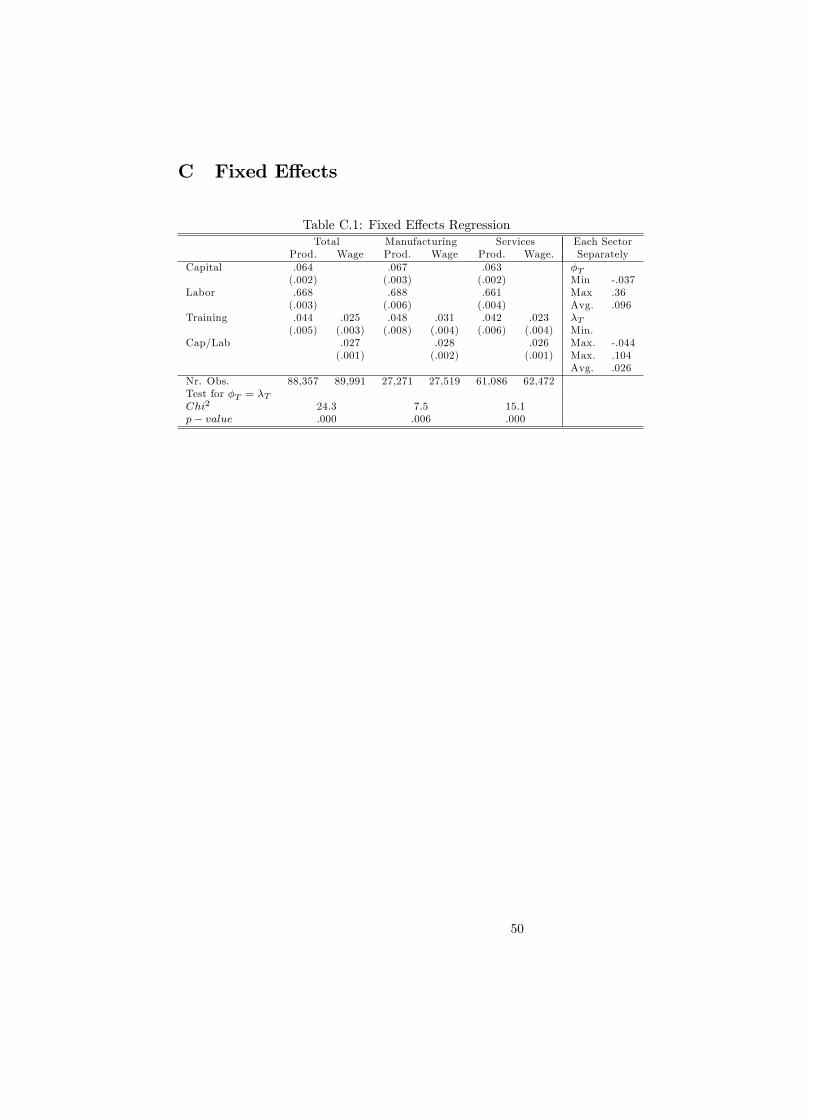
C Fixed E¤ects

Table C.1: Fixed E¤ects RegressionTotal Manufacturing Services Each Sector

Prod. Wage Prod. Wage Prod. Wage. SeparatelyCapital .064 .067 .063 �T

(.002) (.003) (.002) Min -.037Labor .668 .688 .661 Max .36

(.003) (.006) (.004) Avg. .096Training .044 .025 .048 .031 .042 .023 �T

(.005) (.003) (.008) (.004) (.006) (.004) Min.Cap/Lab .027 .028 .026 Max. -.044

(.001) (.002) (.001) Max. .104Avg. .026

Nr. Obs. 88,357 89,991 27,271 27,519 61,086 62,472Test for �T = �TChi2 24.3 7.5 15.1p� value .000 .006 .000

50

Figure C.1: Impact Training on Productivity and Wages: Fixed E¤ects.

14 15

17

20

21

22

24

25

26

27

2829

31

32

33

34

364550

51

52

55

60

63

70

7172

74

0.0

5.1

.15

.2Im

pact

 on 

Pro

duct

ivity

0 .05 .1 .15 .2Impact on Wages

Production function and wage equation estimated with firm fixed effects

Impact Training on Wages and Productivity

51

D Imperfect Substitution between Blue andWhiteCollar Workers; Sector Heterogeneity

Table D.1: Blue collar and white collar workers; per NACE 2 digit sectorBlue Collar White Collar Capital Training Nr. Obs

ACF1 ACF2 ACF1 ACF2 ACF1 ACF2 ACF1 ACF2 Obs Clust

15 Food Products .411 .421 .381 .377 .155 .155 .090 .088 3,191 557(.034) (.108) (.035) (.044) (.021) (.021) (.028) (.030)

17 Textile Products .485 .457 .293 .305 .126 .126 .153 .154 1,509 273(.145) (.252) (.045) (.105) (.021) (.020) (.042) (.046)

18 Wearing Apparel .218 .218 .495 .495 .065 .064 .008 .008 295 58(.610) (.808) (.221) (.273) (.078) (.087) (.156) (.173)

20 Wood Products .261 .232 .404 .414 .068 .069 .340 .345 483 102(.341) (.528) (.109) (.197) (.028) (.030) (.187)

21 Paper Products .540 .512 .357 .371 .088 .091 .090 .093 630 95(.272) (.330) (.105) (.117) (.031) (.036) (.061) (.060)

22 Publishing .233 .417 .064 .145 .116 .103 .081 .096 1,042 194(.335) (.544) (.133) (.171) (.025) (.034) (.078) (.094)

24 Chemical Products .234 .230 .577 .579 .145 .145 .131 .131 1,714 275(.056) (.325) (.053) (.111) (.031) (.035) (.051) (.048)

25 Rubber and Plastic .440 .465 .395 .381 .157 .156 .175 .176 1,331 211(.068) (.225) (.049) (.079) (.019) (.023) (.042) (.049)

26 Mineral Products .464 .462 .349 .350 .082 .082 .138 .138 1,676 284(.064) (.155) (.049) (.051) (.031) (.033) (.041) (.043)

27 Basic Metals .288 .172 .439 .497 .074 .077 .112 .114 893 135(.202) (.399) (.098) (.122) (.041) (.039) (.073) (.068)

28 Metal Products .414 .256 .290 .324 .098 .102 .100 .104 2,426 436(.209) (.303) (.035) (.062) (.018) (.018) (.038) (.038)

29 Machinery .347 .350 .495 .494 .103 .103 .154 .154 1,481 257(.100) (.375) (.081) (.104) (.022) (.027) (.051) (.058)

31 Electrical Machinery .213 .167 .552 .586 .038 .037 .196 .207 587 97(.104) (.315) (.068) (.087) (.026) (.028) (.064) (.068)

33 Medical Eq., Optical Instr. .316 .357 .590 .562 .049 .047 .268 .266 255 49(.166) (.282) (.255) (.259) (.056) (.060) (.133) (.134)

34 Motor Vehicles .619 .630 .272 .264 .068 .067 .137 .140 640 112(.135) (.248) (.115) (.120) (.033) (.033) (.072) (.081)

36 Furniture, Manuf. n.e.c. .449 .406 .344 .364 .073 .072 .079 .081 898 157(.239) (.651) (.096) (.135) (.034) (.036) (.055) (.090)

Results ACF method with contemporaneous blue collar workers (ACF1) and blue collar workers lagged one period asinstruments. Standard errors are computed using a block bootstrap procedure with 500 replications and are robustagainst heteroskedasticity and intra-group correlation

52

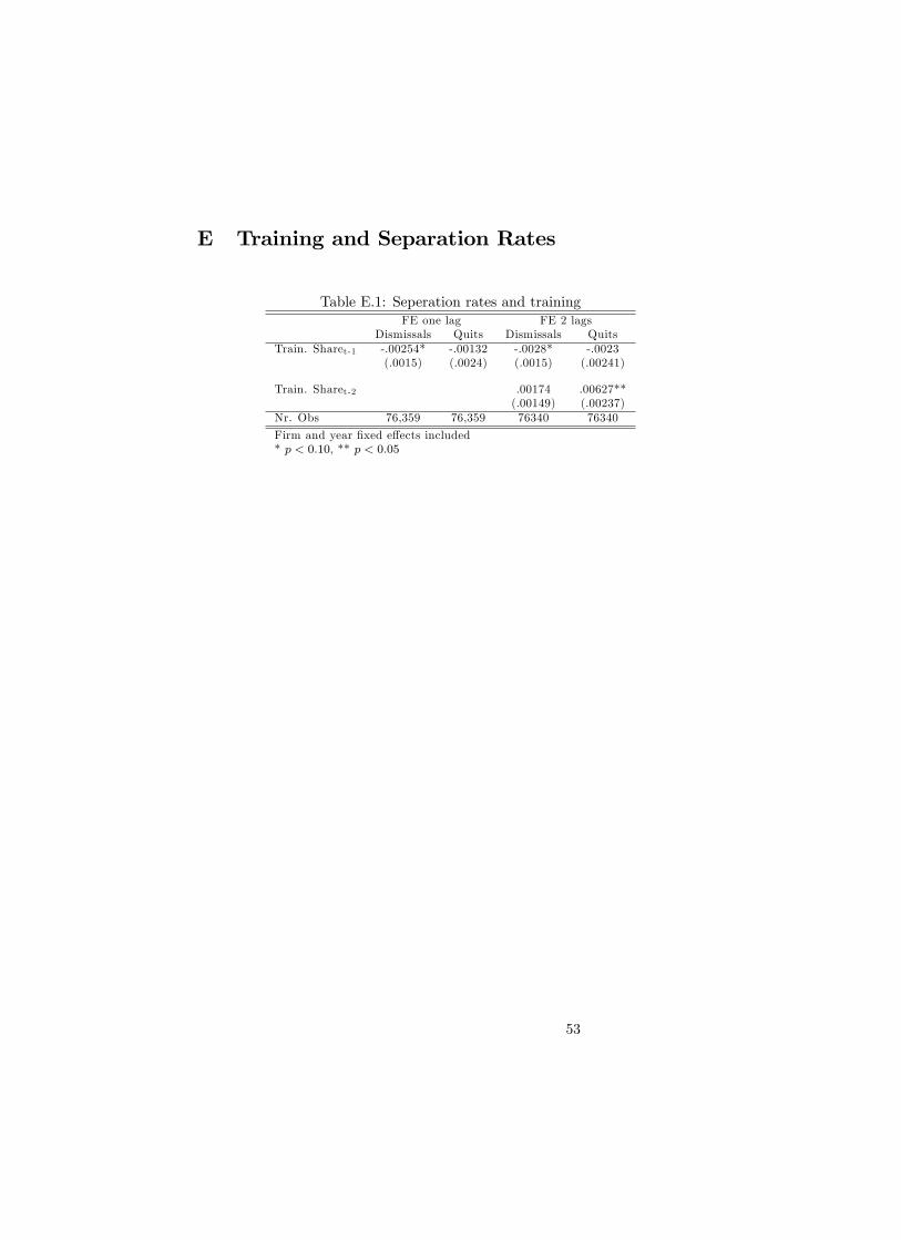
E Training and Separation Rates

Table E.1: Seperation rates and trainingFE one lag FE 2 lags

Dismissals Quits Dismissals QuitsTrain. Sharet-1 -.00254* -.00132 -.0028* -.0023

(.0015) (.0024) (.0015) (.00241)

Train. Sharet-2 .00174 .00627**(.00149) (.00237)

Nr. Obs 76,359 76,359 76340 76340

Firm and year �xed e¤ects included* p < 0:10, ** p < 0:05

53