The Impact of the 2005 CAP-First Pillar Reform (FPR) as a ... Impact of the 2005 CAP-First Pillar...
20
The Impact of the 2005 CAP-First Pillar Reform (FPR) as a Multivalued Treatment Effect Alternative Estimation Approaches Roberto Esposti Department of Economics and Social Sciences Università Politecnica delle Marche Ancona (Italy) Alghero, 26/06/2014
Transcript of The Impact of the 2005 CAP-First Pillar Reform (FPR) as a ... Impact of the 2005 CAP-First Pillar...
The Impact of the 2005 CAP-First Pillar Reform (FPR) as a Multivalued Treatment EffectAlternative Estimation Approaches
Roberto Esposti
Department of Economics and Social SciencesUniversità Politecnica delle Marche Ancona (Italy)
Alghero, 26/06/2014

2| R. Esposti, 26 June 2014
OUTLINE
Objective: Is the increasingly complex TE econometrics toolkit suitable for “complex” policy treatments like the FPR? By the way: about 40 bil €/year (30% of EU
budget)
1. The FPR case: methodological challenges
2. MT-ATE alternative estimation approaches
3. Results
4. Concluding remarks

3| R. Esposti, 26 June 2014
1. FPR: methodological challenges (1/5)
What is needed to recreate such a quasi-experimentalsituation and identify/estimate the Avg. TE (ATE):
Requirements Issues
A clear treatment (T) - Multiple treatments- Multivalued treatments
A clear objective (Y) - Unclear (undeclared) outcome/target variable- Multiple objectives
A clear counterfactual (T = 0) - No counterfactuals- Unsuitable counterfactuals
Observable confoundingvariables (X)
- Controlling for (un)observables- Proper matching
2
1
2

4| R. Esposti, 26 June 2014
1. FPR: methodological challenges (2/5)
Objective – Estimate the TE of FPR→ The treatment: the 2003/2005 Reform of the First Pillar of the CAP (FPR)
• Decoupling of support: the key of the reform
– Reorientation to market:
Let farmers choose what (and if) to produce
Let farmers achieve an higher allocative efficiency
Objective/Expected outcome: change in the production mix of farmers receiving the treatment

5| R. Esposti, 26 June 2014
1. FPR: methodological challenges (3/5)
Why don’t use powerful TE econometrics to assess the impact of the FPR?– We have micro-data!
The sample: a balanced panel (constant sample) of 6542 farms obs. over years 2003-2007 (pre and post-reform).
– But:
1. CAP is a multioutcome policy
2. CAP is a multitreatment policy
3. CAP is a multivalued treatment
4. No suitable counterfactuals for the FPR

6| R. Esposti, 26 June 2014
1. FPR: methodological challenges (4/5)
FPR as a multioutcome policy: How do we measure if and to what extent farms changed their output vector?
– Two different types of outcome (i-th farm):
• In a short-run perspective: change in the composition of output (K
is the of possible production activities; sk the respective share on
GPV). Measures of distance between pre (A) and post (B)
• In a long-run perspective: investment decisions (I = investments;
VA = Value Added)
K
k
AikBiki ssy1
2
,,
1Output-distanceindex
Ai
Ai
Bi
Bi
iVA
I
VA
Iy
,
,
,
,4Investment rate
Alternative:
y2 simply counts
the changes in
the output vector
Alternative:
y3 investments in
absolute values
Note: the outcome/target variable is ALREADY a difference. The TE is a difference in the difference
1

7| R. Esposti, 26 June 2014
1. FPR: methodological challenges (5/5)
FPR as a Multivalued Treatment (MT) →Treatment Intensity (TI) = FPs/GPV
5430 treated farms
1112 non-treated farms
Can’t they be suitable counterfactuals for the FPR? Eligibility to FPR depends on
production choices made in
the 2000-2002 period. If they
made very peculiar choices
they must be peculiar
But with MT we do not
need counterfactuals
Distribution of the continuous treatment (TI), First Pillar support on farm’s GPV (in %): Kernel density (K)
and frequency histogram (avg. over 2003-2007 period)
17%
26%
17%
12%
10%
7%
4%3%
2% 1% 1% 1%0%
5%
10%
15%
20%
25%
30%
= 0 0-5% 5-10% 10-15% 15-20% 20-25% 25-30% 30-35% 35-40% 40-45% 45-50% >50%
First Pillar support on GPV
0
.02
.04
.06
.08
Density
0 20 40 60 80
First Pillar Support on GPV
K
2

8| R. Esposti, 26 June 2014
2. MT-ATE estimation approaches (1/4)
3 POSSIBLE EMPIRICAL STRATEGIES:
1st strategy – PSM-ATT: binary treatment; counterfactuals foundthrough matching conditional on a set of covariates
Selection-on-unobservables bias still a problem
2nd strategy – DID-ATT: binary treatment, counterfactuals are thetreated observations themselves before the treatment, still non-treatedare needed to get rid of the effects of time
Selecting the baseline and the follow-up obs. (years) is critical→ CIIA and placebo testing
3rd strategy – MT-ATE: the treatment is a continuous/discretevariable, a relationship between the treatment level and theoutcome variable can be estimated (the DRF); non-treated units(counterfactuals) are not needed→which is the effect for atreated unit of receiving an higher (lower) treatment level?

9| R. Esposti, 26 June 2014
2. MT-ATE estimation approaches (2/4)
Hirano-Imbens approach - Start with the Rubin (1974) intuition:
Define a set of potential outcomes {Yi(T)}TΞ where Ξ is the
set of potential treatment levels and Yi(T) is a random
variable that maps, for the i-th unit, a particular potential
treatment, T, to the potential outcome Y
However, for any i-th only one Yi is observed
corresponding to the actual treatment level Ti
The approach estimates the function linking Y=f(T) on
average: the average Dose-Response Function (aDRF)
It is a 4-step parametric estimation approach

10| R. Esposti, 26 June 2014
2. MT-ATE estimation approaches (3/4)
Hirano-Imbens approach - Estimation:
1st step: the GPS estimation:
Probability of the i-th unit to receive the treatment level Ti
2nd and 3rd steps: the uDRF and aDRF estimation
Estimation of the conditional expectation of the potential outcome with respect to T and the estimated GPS: a fully interacted flexible function (K,H-th order polynomial) then averaged for any given T
4th step: the ATE estimation
2,, iiiiii N~TTrGPS XβXX
1ˆˆorˆ
jjjjj FRaDFRaDATETFRaDATE

11| R. Esposti, 26 June 2014
2. MT-ATE estimation approaches (4/4)
The Cattaneo alternative (1): Hirano-Imbens approach: computationally complex and too arbitrary
parametric assumptions
Cattaneo (2010) approach: a semiparametric estimation
Discrete instead of continuous treatment
A 3-step approach:
The first step is common: GPS estimation (but now is a MLM)
The second step is a semiparametric estimation: based on the estimated GPS, the potential outcome means for any treatment level (µj) are estimated imposing a set of moment restrictions
Two asymptotically equivalent alternatives (the latter is preferable in finite sample):
IPW (Inverse Probability Weighting) Estimation
EIF (Efficient Influence Function) Estimation
The third step consists in estimating the ATE
1,,,/ˆˆ
jIPWjIPWjEIFIPWATE

12| R. Esposti, 26 June 2014
3. Results of the application (1/7)
Covariates - Three (+1) groups of confounding factors:
Individual characteristics of the farmer (AGE) and of thefarm (Altitude - ALT).
Economic (ES, FC) and physical (AWU, HP, UAA and, at leastpartially, LU) size of the farm clearly matters.
Variables directly expressing the production specialization ofthe farm(TF and, in part, LU) .
A final confounding variable included in the analysis is thedummy expressing second pillar support (RDP) (1766 farms;27%)
skip

13| R. Esposti, 26 June 2014
3. Results of the application (2/7)
MT estimation - Hirano-Imbens: aDRF and TE
y1
-1-.
50
.51
E[y
1(t
)]
0 20 40 60 80
Treatment level
Dose Response Lower bound Higher bound
Dose Response Function
-.1
0.1
.2.3
.4
E[y
1(t
+1
)]-E
[y1(t
)]
0 20 40 60 80
Treatment level
Treatment Effect Lower bound Higher bound
Treatment Effect Function

14| R. Esposti, 26 June 2014
3. Results of the application (3/7)
MT estimation - Hirano-Imbens: aDRF and TE
y2
.00
5.0
1.0
15
.02
.02
5
E[y
2(t
)]
0 20 40 60 80
Treatment level
Dose Response Lower bound Higher bound
Dose Response Function
0
.00
2.0
04
.00
6.0
08
E[y
2(t
+1
)]-E
[y2
(t)]
0 20 40 60 80
Treatment level
Treatment Effect Lower bound Higher bound
Treatment Effect Function

15| R. Esposti, 26 June 2014
3. Results of the application (4/7)
MT estimation - Hirano-Imbens: aDRF and TE
y3
-50
00
0
0
500
00
100
00
01
50
00
0
E[y
3(t
)]
0 20 40 60 80
Treatment level
Dose Response Lower bound Higher bound
Dose Response Function
-20
00
0-1
000
0
0
100
00
200
00
300
00
E[y
3(t
+1
)]-E
[y3
(t)]
0 20 40 60 80Treatment level
Treatment Effect Lower bound Higher bound
Treatment Effect Function

16| R. Esposti, 26 June 2014
3. Results of the application (5/7)
MT estimation - Hirano-Imbens: aDRF and TE
y4
-.5
0.5
1
E[y
4(t
)]
0 20 40 60 80
Treatment level
Dose Response Lower bound Higher bound
Dose Response Function
-.3
-.2
-.1
0.1
E[y
4(t
+1)]
-E[y
4(t
)]
0 20 40 60 80
Treatment level
Treatment Effect Lower bound Higher bound
Treatment Effect Function
17| R. Esposti, 26 June 2014
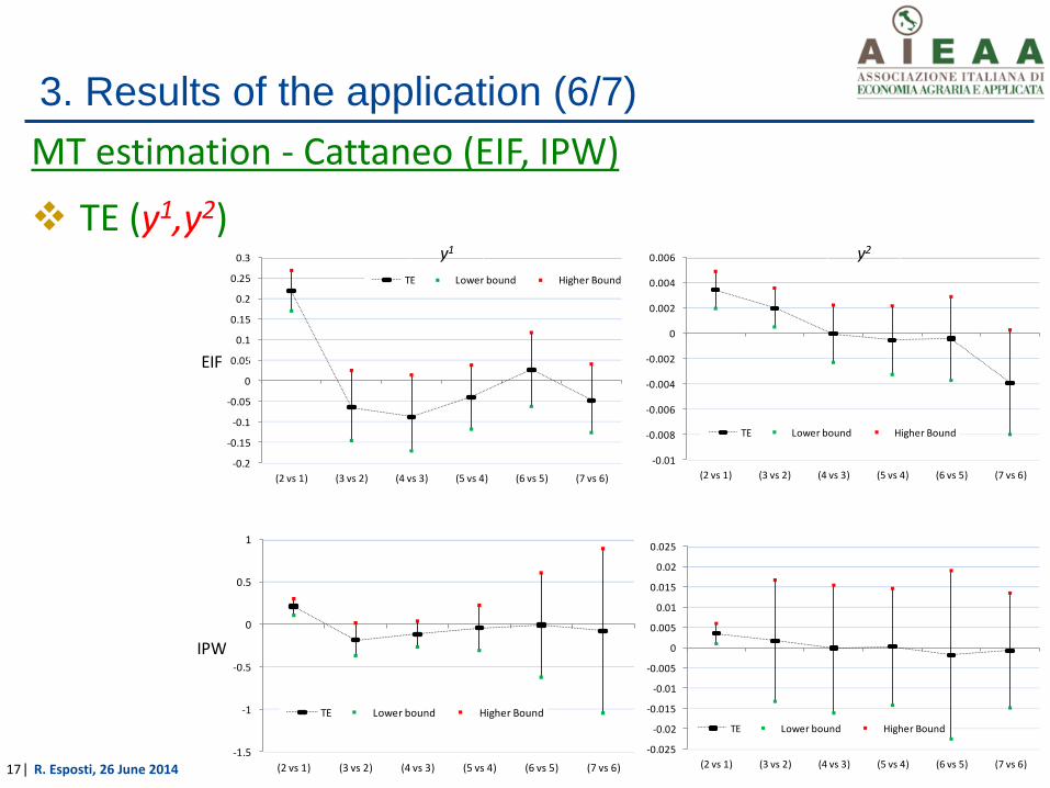
3. Results of the application (6/7)
MT estimation - Cattaneo (EIF, IPW)
TE (y1,y2)
-0.2
-0.15
-0.1
-0.05
0
0.05
0.1
0.15
0.2
0.25
0.3
(2 vs 1) (3 vs 2) (4 vs 3) (5 vs 4) (6 vs 5) (7 vs 6)
TE Lower bound Higher Bound
-0.01
-0.008
-0.006
-0.004
-0.002
0
0.002
0.004
0.006
(2 vs 1) (3 vs 2) (4 vs 3) (5 vs 4) (6 vs 5) (7 vs 6)
TE Lower bound Higher Bound
-1.5
-1
-0.5
0
0.5
1
(2 vs 1) (3 vs 2) (4 vs 3) (5 vs 4) (6 vs 5) (7 vs 6)
TE Lower bound Higher Bound
-0.025
-0.02
-0.015
-0.01
-0.005
0
0.005
0.01
0.015
0.02
0.025
(2 vs 1) (3 vs 2) (4 vs 3) (5 vs 4) (6 vs 5) (7 vs 6)
TE Lower bound Higher Bound
y1 y2
EIF
IPW

18| R. Esposti, 26 June 2014
3. Results of the application (7/7)
MT estimation - Cattaneo (EIF, IPW)
TE (y3,y4)
-80000
-60000
-40000
-20000
0
20000
40000
60000
(2 vs 1) (3 vs 2) (4 vs 3) (5 vs 4) (6 vs 5) (7 vs 6)
TE Lower bound Higher Bound
-0.05
0
0.05
0.1
0.15
0.2
(2 vs 1) (3 vs 2) (4 vs 3) (5 vs 4) (6 vs 5) (7 vs 6)
TE Lower bound Higher Bound
-150000
-100000
-50000
0
50000
100000
150000
(2 vs 1) (3 vs 2) (4 vs 3) (5 vs 4) (6 vs 5) (7 vs 6)
TE Lower bound Higher Bound
y3 y4
EIF
IPW
-0,8
-0,6
-0,4
-0,2
0
0,2
0,4
0,6
0,8
1
(2 vs 1) (3 vs 2) (4 vs 3) (5 vs 4) (6 vs 5) (7 vs 6)
TE Lower bound Higher Bound

19| R. Esposti, 26 June 2014
4. Concluding remarks
Did the FPR reoriented production decisions? YES Short-run vs. Long-run production decisions
– FPR affected SR production decisions– SR changes seem conservative: +in number of products, - in GPV shares– SR impact is lower (or null) for higher treatment levels: lock-in effect?– Impact on LR (inv.) decisions is questionable– LR impact (if any) is higher for higher treatment levels: pure financial effect?– LR impact may come from the complementarity of the two pillars
• Multitreatment effects? Pros and cons of the MT estimation approaches
– Advantages on PSM-ATT and DID-ATT estimation : no need of counterfactuals (non-treated units) take the continuous nature of the treatment into account more robust
– MT-ATT estimation complex and based on arbitrary assumptions Results of good quality with the Hirano-Imbens approach Cattaneo approach: poorer results (especially with IPW estimation)
pros
cons

20| R. Esposti, 26 June 2014
Thanks for your attention