THE IMPACT OF TAXES AND SOCIAL SPENDING ON...

By Nora Lustig, George Gray-Molina, Sean Higgins, Miguel Jaramillo, Wilson Jiménez,

Veronica Paz, Claudiney Pereira, Carola Pessino, John Scott, and Ernesto Yañez

THE IMPACT OF TAXES AND SOCIAL

SPENDING ON INEQUALITY AND

POVERTY IN ARGENTINA, BOLIVIA,

BRAZIL, MEXICO AND PERU:

A SYNTHESIS OF RESULTS

Working Paper No. 3

August 2012

2

The Impact of Taxes and Social Spending on Inequality and Poverty in Argentina,

Bolivia, Brazil, Mexico and Peru: A Synthesis of Results

Nora Lustig, George Gray-Molina, Sean Higgins, Miguel Jaramillo, Wilson Jiménez, Veronica

Paz, Claudiney Pereira, Carola Pessino, John Scott and Ernesto Yañez*

CEQ Working Paper August 2012

ABSTRACT

We apply a standard tax and benefit incidence analysis to estimate the impact on inequality and poverty of direct taxes, indirect taxes and subsidies, and social spending (cash and food transfers and in-kind transfers in education and health). The extent of inequality reduction induced by direct taxes and transfers is rather small (2 percentage points on average) especially when compared with that found in Western Europe (15 percentage points on average). What prevents Argentina, Bolivia and Brazil from achieving similar reductions in inequality is not the lack of revenues but the fact that they spend less on cash transfers –especially transfers that are progressive in absolute terms--as a share of GDP. Indirect taxes result in that net contributors to the fiscal system start at the fourth, third and even second decile on average, depending on the country. When in-kind transfers in education and health are added, however, the bottom six deciles are net recipients. The impact of transfers on inequality and poverty reduction could be higher if spending on direct cash transfers that are progressive in absolute terms is increased, leakages to the nonpoor are reduced and coverage of the extreme poor by direct transfer programs is expanded. Keywords: fiscal incidence, inequality, poverty, taxes, social spending, Latin America JEL CODES: D31, D63, H11, H22, H5, I14, I24, I3, O15

* Director: Nora Lustig, Tulane University and CGD and IAD; Coordinator: Sean Higgins, Tulane University; Research Assistants: Veronica Argudo, Samantha Greenspun, Katharina Hammler, Juan Carlos Monterrey, Adam Ratzlaff, Emily Travis and Dustin Wonnell, Tulane University, New Orleans, USA. Country Teams: Argentina: Carola Pessino, CGD, Washington, DC and CEMA, Buenos Aires, Argentina; Bolivia: George Gray Molina, UNDP, New York, USA and Wilson Jiménez Pozo, Verónica Paz Arauco and Ernesto Yañez, Instituto Alternativo, La Paz; Bolivia; Brazil: Claudiney Pereira and Sean Higgins, Tulane University; Mexico: John Scott, CIDE and CONEVAL, Mexico City, Mexico and Research Assistant: Francisco Islas; Peru: Miguel Jaramillo, GRADE, Lima, Peru; Research Assistant: Barbara Sparrow. The authors are grateful to James Alm, Armando Barrientos, Lucila Berniell, Otaviano Canuto, Ludovico Feoli, Francisco Ferreira, Ariel Fiszbein, Peter Hakim, Santiago Levy, Luis F. Lopez-Calva, Daniel Ortega, Jeff Puryear, Jamele Rigolini, Pablo Sanguinetti and Ana Maria Sanjuan for their very valuable comments on an earlier draft. All errors remain our sole responsibility.

3

1. INTRODUCTION Latin America is the region with the highest degree of inequality (Ferreira and Ravallion, 2008). Poverty rates – although not the highest by far – are too high for its level of development (IDB, 2011, p. 43). Given these two facts, the extent to which governments use their power to tax and spend to attenuate inequality and poverty is of great importance.1 How much inequality and poverty reduction does Latin America accomplish through taxes and social spending? How progressive are revenue collection and social spending? In order to answer these questions we apply standard incidence analysis to estimate the impact on inequality and poverty (hereafter also called redistribution) of direct taxes2, indirect taxes and subsidies, and social spending (here defined to include cash and food transfers and in-kind transfers in education and health). 3 In the same vein as Breceda et al. (2008, p. 7) we “... aspire to determine the broad distributional patterns of actual tax payments and social spending across income groups.” It is important to emphasize that the analysis presented here relies on standard incidence analysis without behavioral, lifecycle or general equilibrium effects. The analysis does not look into the macroeconomic sustainability of taxation and social spending patterns either. In addition, it focuses on average incidence rather than incidence at the margin. Finally, it excludes some important taxes/other revenues (corporate and international trade taxes, for example) and spending categories (infrastructure investments including urban services and rural roads that benefit the poor, for example) that surely affect income distribution and poverty. Nonetheless, the individual studies reported here are among the most detailed and comparable for Latin American countries to date. Compared to some of the existing studies, reliance on secondary sources is kept to a minimum.4 Readers will note that great care is placed in defining income concepts and specifying the method followed to estimate the incidence of every tax and benefit category in each country. The paper is organized as follows. Section 1 presents a brief description of the income concepts, the definitions of progressiveness and effectiveness, the methods followed to calculate the incidence of taxes and benefits, and the data used in the incidence analysis. Section 2 summarizes the main results and compares them across the five countries. Section 3 concludes. The Appendix presents the definition of income concepts in formulas.

1 See, for example, Birdsall et al. (2008). 2 Taxes include social security contributions in the benchmark analysis. 3In the benchmark analysis contributory pensions are included under market (pre-tax/transfers) income while they are treated as a transfer in the sensitivity analysis.4 Breceda et al. (2008) and Goñi et al. (2011) rely heavily on secondary sources for their incidence analysis.

4

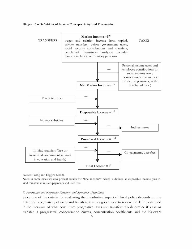
2. CONCEPTS, DEFINITIONS, AND DATA5 i. Market, Net Market, Disposable, Post-fiscal and Final Income: Definitions and Measurement As usual, any incidence study must start by defining the basic income concepts. In our study we use five: market, net market, disposable, post-fiscal and final income. The categories included in each concept are shown in Diagram 1. One area in which there is no agreement is how pensions from a pay-as-you-go contributory system should be treated. Arguments exist in favor of both treating contributory pensions as part of market income because they are deferred income (Breceda et al., 2008; Immervoll et al., 2009) and treating them as a government transfer, especially in systems with a large subsidized component (Goñi et al., 2011; Immervoll et al., 2009; Lindert et al., 2006; Silveira et al., 2011). Since this is an unresolved issue, in our study we defined a benchmark case in which contributory pensions are part of market income. We also did a sensitivity analysis where pensions are classified under government transfers.6 We found that the progressivity of government transfers changes to more or less progressive depending on the country. Contributory pensions are regressive only in Peru and in the other four countries they are progressive (in absolute and relative terms). Overall, the impact on inequality and poverty of adding contributory pensions to social spending is small and qualitative results are not affected. The results presented here are for the benchmark analysis. Results for the case when pensions are placed under government transfers can be seen in the Statistical Appendix, available upon request.

5 For more details on concepts and definitions, see Lustig and Higgins (2012). 6 Immervoll et al. (2009) do the analysis under these two scenarios as well.

5

Diagram 1 – Definitions of Income Concepts: A Stylized Presentation

Source: Lustig and Higgins (2012). Note: in some cases we also present results for “final income*” which is defined as disposable income plus in-kind transfers minus co-payments and user fees.

ii. Progressive and Regressive Revenues and Spending: Definitions Since one of the criteria for evaluating the distributive impact of fiscal policy depends on the extent of progressivity of taxes and transfers, this is a good place to review the definitions used in the literature of what constitutes progressive taxes and transfers. To determine if a tax or transfer is progressive, concentration curves, concentration coefficients and the Kakwani

Market Income =I! Wages and salaries, income from capital, private transfers; before government taxes, social security contributions and transfers; benchmark (sensitivity analysis) includes (doesn’t include) contributory pensions

TRANSFERS TAXES

Direct transfers

Net Market Income= I!

Disposable Income = I!

Personal income taxes and employee contributions to

social security (only contributions that are not

directed to pensions, in the benchmark case)

−

+

Indirect subsidies + − Indirect taxes

Post-fiscal Income = I!"

In-kind transfers (free or subsidized government services

in education and health)

+ − Co-payments, user fees

Final Income = I!

6

(1977) index are commonly used.

Concentration curves are constructed similarly to Lorenz curves but the difference is that the vertical axis measures the proportion of the tax (transfer) under analysis paid (received) by each quantile. Therefore, concentration curves (for a transfer targeted to the poor, for example) can be above the diagonal (something that, by definition, could never happen with a Lorenz curve). Concentration coefficients are calculated in the same manner as is the Gini; for cases in which the concentration coefficient is above the diagonal, the difference between the triangle of perfect equality and the area under the curve is negative, which cannot occur with the Gini for the income distribution by definition. The data used to generate concentration curves and coefficients are derived from incidence analyses.

In the literature there is no agreement on when to label a transfer as ‘progressive.’ The progressivity/regressivity of a transfer can be measured in absolute terms, by comparing the per capita transfers between quantiles, or in relative terms, by comparing transfers as a percentage of the income of each quantile. Some authors label a transfer as progressive only when the per capita amount decreases with income (e.g., Scott, 2011). Others, when the proportion received (as a percentage of market income) decreases with income (e.g., Lindert et al., 2006; O’Donnell et al., 2008). Here, we have opted for the latter definition. This is consistent with an intuitively appealing principle: a transfer or tax is defined as progressive (regressive) if it results in a less (more) unequal distribution than that of market income.

In particular:7

1. A tax is progressive (regressive) if the proportion paid – in relation to market income – increases (decreases) as income rises. The concentration coefficient is positive and larger (smaller) than the market income Gini. The Kakwani index, defined for taxes as the tax concentration coefficient minus the market income Gini, will be positive (negative) if a tax is progressive (regressive).

2. A transfer is progressive (regressive) in relative terms if the proportion received

– in relation to market income – decreases (increases) as income rises. The concentration coefficient will be positive and lower (higher) than the market income Gini. The Kakwani index, defined for transfers as the market income Gini minus the transfer’s concentration

7 Our taxonomy of absolute and relative progressivity is similar to that used by Lindert et al. (2006). The taxonomy in O’Donnell et al. (2008) is slightly different: they refer to relative progressivity as “progressivity, or weak progressivity” and to absolute progressivity as “absolute or strong progressivity” (p. 185).

7

coefficient, will be positive (negative) if a transfer is progressive (regressive) in relative terms.8 3. A transfer will be progressive in absolute terms if the per capita amount

received increases as income rises. The concentration coefficient will be negative. The Kakwani index will be positive and higher than the market income Gini if a transfer is progressive in absolute terms.

4. A tax or transfer will be neutral (in relative terms) if the distribution of the tax or the transfer coincides with the distribution of market income. The concentration coefficient will be equal to the market income Gini. The Kakwani index will equal zero if a tax or transfer is neutral. The four cases are illustrated graphically in Diagram 2.

Diagram 2 - Concentration Curves for Progressive and Regressive Transfers (Taxes)

Source: Lustig and Higgins (2012).

8 The index originally proposed by Kakwani (1977) only measures the progressivity of taxes. It is defined as the tax’s concentration coefficient minus the market income Gini. To adapt to the measurement of transfers, Lambert (1985) suggests that in the case of transfers it should be defined as market income Gini minus the concentration coefficient (i.e., the negative of the definition for taxes) to make the index positive whenever the change is progressive.

8

iii. Allocating Taxes and Transfers at the Household Level Unfortunately the information on direct and indirect taxes, transfers in cash and in-kind and subsidies cannot always be obtained directly from household surveys. When it can be obtained, we call this the Direct Identification Method. When the direct method is not feasible, one can use the inference, simulation or imputation methods (described in more detail below). As a last resort, one can use secondary sources. Direct Identification Method On some surveys, questions specifically ask if households received benefits from (paid taxes to) certain social programs (tax and social security systems), and how much they received (paid). When this is the case, it is easy to identify transfer recipients and taxpayers, and add or remove the value of the transfers and taxes from their income, depending on the definition of income being used. Inference Method Unfortunately, not all surveys have the information necessary to use the direct identification method. In some cases, transfers from social programs are grouped with other income sources (in a category for “other income,” for example). In this case, it might be possible to infer which families received a transfer based on whether the value they report in that income category matches a possible value of the transfer in question. Simulation Method In the case that neither the direct identification nor the inference method can be used, transfer benefits can sometimes be simulated, determining beneficiaries (taxpayers) and benefits received (taxes paid) based on the program (tax) rules. For example, in the case of a conditional cash transfer that uses a proxy means test to identify eligible beneficiaries, one can replicate the proxy means test using survey data, identify eligible families, and simulate the program’s impact. However, this method gives an upper bound, as it assumes perfect targeting and no errors of inclusion or exclusion. In the case of taxes, estimates usually make assumptions about informality and evasion. Imputation Method The imputation method is a mix between the direct identification and simulation methods; it uses some information from the survey, such as the respondent reporting attending public school or receiving a direct transfer in a survey that does not ask for the amount received, and some information from either public accounts, such as per capita public expenditure on education by level, or from the program rules.

9

The four methods described above rely on at least some information directly from the household survey being used for the analysis. As a result, some households receive benefits, while others do not, which is an accurate reflection of reality. However, in some cases the household survey analyzed lacks the necessary questions to assign benefits to households. In this case, there are two additional methods. Alternate Survey When the survey lacks the necessary questions, such as a question on the use of health services or health insurance coverage (necessary to impute the value of in-kind health benefits to households), an alternate survey may be used by the author to determine the distribution of benefits. In the alternate survey, any of the four methods above could be used to identify beneficiaries and assign benefits. Then, the distribution of benefits according to the alternate survey is used to impute benefits to all households in the primary survey analyzed; the size of each household’s benefits depends on the quantile to which the household belongs. Note that this method is more accurate than the secondary sources method below, because although the alternate survey is somewhat of a “secondary source,” the precise definitions of income and benefits used in CEQ can be applied to the alternate survey. Secondary Sources Method When none of the above methods are possible, secondary sources that provide the distribution of benefits (taxes) by quantile may be used. These benefits (taxes) are then imputed to all households in the survey being analyzed; the size of each household’s benefits (taxes) depends on the quantile to which the household belongs. The method used by each country and for each component of fiscal policy is mentioned in Table 2 under the corresponding column; more detail is provided in Statistical Appendix available upon request. iv. Redistributive Effectiveness Indicator The Effectiveness Indicator is defined as the effect on inequality or poverty of the transfers being analyzed divided by their size relative to GDP. For example, for direct transfers, the effectiveness indicator is the reduction between the net market income and disposable income Ginis as a percent of the net market income Gini, divided by the size of direct transfers (only those included in the incidence analysis) as a percent of GDP. Although the size of direct transfers is measured by budget size according to national accounts, only direct transfer programs that are captured by the survey (or otherwise estimated by the authors) are included, since they are the only programs that can lead to an observed change in income.

10

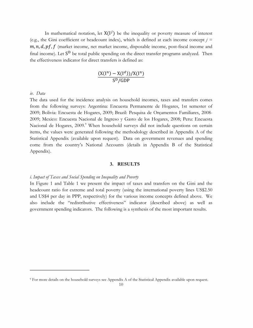
In mathematical notation, let X(I!) be the inequality or poverty measure of interest (e.g., the Gini coefficient or headcount index), which is defined at each income concept j = 𝑚,𝑛,𝑑,𝑝𝑓, 𝑓 (market income, net market income, disposable income, post-fiscal income and final income). Let S! be total public spending on the direct transfer programs analyzed. Then the effectiveness indicator for direct transfers is defined as:

X I! − X(I! )/X(I!)

S!/GDP

iv. Data The data used for the incidence analysis on household incomes, taxes and transfers comes from the following surveys: Argentina: Encuesta Permanente de Hogares, 1st semester of 2009; Bolivia: Encuesta de Hogares, 2009; Brazil: Pesquisa de Orçamentos Familiares, 2008-2009; Mexico: Encuesta Nacional de Ingreso y Gasto de los Hogares, 2008; Peru: Encuesta Nacional de Hogares, 2009.9 When household surveys did not include questions on certain items, the values were generated following the methodology described in Appendix A of the Statistical Appendix (available upon request). Data on government revenues and spending come from the country’s National Accounts (details in Appendix B of the Statistical Appendix).

3. RESULTS

i. Impact of Taxes and Social Spending on Inequality and Poverty In Figure 1 and Table 1 we present the impact of taxes and transfers on the Gini and the headcount ratio for extreme and total poverty (using the international poverty lines US$2.50 and US$4 per day in PPP, respectively) for the various income concepts defined above. We also include the “redistributive effectiveness” indicator (described above) as well as government spending indicators. The following is a synthesis of the most important results.

9 For more details on the household surveys see Appendix A of the Statistical Appendix available upon request.

11

Figure 1 – Gini Coefficient and Headcount Ratio for Each Income Concept Gini Coefficient

Headcount Ratio

Source: Authors’ calculations based on household surveys and public accounts. Note: The Gini for final income in Peru cannot be compared with the others because health spending in Peru’s analysis is only a fraction of public spending on health due to data limitations.

12

Table 1 - Gini, Headcount Ratio and Redistributive Effectiveness: Argentina, Bolivia, Brazil, Mexico and Peru

Source: Authors’ calculations based on household surveys and public accounts. Notes: Peru not comparable with other countries because health spending includes only a fraction of public spending on health due to data limitations. "% change wrt" is an abbreviation for "percent change with respect to". The Effectiveness Indicator is defined as the redistributive effect of the taxes or transfers being analyzed divided by their relative size. Specifically, it is defined as follows: For the disposable income Gini and headcount index, it is the fall between the net market income and disposable income Gini/headcount index as a percent of the net market income Gini/headcount index, divided by the size of direct transfers (only including programs included in the analysis) as a percent of GDP. For the final income* Gini, it is the fall between the net market income and final income* Gini as a percent of the final income* Gini, divided by the size of the sum of direct transfers, education spending, health spending, and (where it was included in the analysis) housing and urban spending, as a percent of GDP. In this table the headcount index is expressed as a percentage. Not available means that the corresponding figure could not be estimated based on the household survey being used. Not applicable indicates that market income is not applicable in Bolivia because there were negligible or no direct

MarketIncome

NetMarketIncome

DisposableIncome

Post‐fiscalIncome

FinalIncome

GNI/cap.inPPP‐yrofsurvey(US$)(rank)

Primaryspendingasa%ofGDP(rank)

CEQSocialSpendingas%ofGDP(excludingcontributorypensions)

DirectTransfersasa%ofGDP(rank)

ConcentrationCoefficientforSocialSpending(rank;lowest/mostprogressivetohighes/leastprogressivet)

ColumnNumber [1] [2] [3] [4] [5] [6] [7] [8] [9] [10]

Gini 0.503 0.498 0.465 0.480 0.388 $14,030 37.57% 15.78% 3.08% ‐0.14

%changewrtmarketincome ‐‐ ‐0.9% ‐7.6% ‐4.5% ‐22.8% 2 large 2 2 2

%changewrtnetmarketincome ‐‐ ‐‐ ‐6.7% ‐3.6% ‐22.1%

Effectivenessindicator ‐‐ ‐‐ 2.18 ‐‐ ‐‐

Headcountindex($4PPP) Notavailable 23.0% 14.0% Notavailable%changewrtnetmarketincome ‐‐ ‐‐ ‐39.1%

Effectivenessindicator ‐‐ ‐‐ 12.70 ‐‐

Headcountindex($2.5PPP) Notavailable 13.9% 5.0% Notavailable

%changewrtnetmarketincome ‐‐ ‐‐ ‐64.0%Effectivenessindicator ‐‐ ‐‐ 20.79 ‐‐

Gini Notapplicable 0.477 0.468 0.475 0.425 $4,621 44.86% 13.67% 2.14% 0.12%changewrtnetmarketincome ‐‐ ‐‐ ‐1.9% ‐0.4% ‐10.9% 5 large 3 3 5


Headcountindex($4PPP) Notapplicable 29.4% 27.2% 29.6%

%changewrtnetmarketincome ‐‐ ‐‐ ‐7.3% 1.0%


Headcountindex($2.5PPP) Notapplicable 15.1% 13.5% 15.5%

%changewrtnetmarketincome ‐‐ ‐‐ ‐10.7% 2.4%Effectivenessindicator ‐‐ ‐‐ 4.99 ‐‐

Gini 0.573 0.562 0.542 0.539 0.459 $10,372 36.85% 16.17% 4.15% ‐0.09

%changewrtmarketincome ‐‐ ‐1.9% ‐5.5% ‐6.0% ‐19.9% 3 large 1 1 3


Effectivenessindicator ‐‐ 0.87 ‐‐ ‐‐

Headcountindex($4PPP) 26.6% 26.8% 23.6% 28.5%

%changewrtnetmarketincome ‐‐ ‐‐ ‐12.0% 6.3%


Headcountindex($2.5PPP) 15.3% 15.4% 11.9% 15.0%

%changewrtnetmarketincome ‐‐ ‐‐ ‐22.6% ‐2.3%Effectivenessindicator ‐‐ ‐‐ 5.44 ‐‐

Gini 0.549 0.539 0.532 0.524 0.482 $14,530 21.87% 8.06% 0.74% ‐0.17

%changewrtmarketincome ‐‐ ‐1.8% ‐3.1% ‐4.6% ‐12.2% 1 small 4 4 1


Effectivenessindicator ‐‐ 1.75 ‐‐ ‐‐


%changewrtnetmarketincome ‐‐ ‐‐ ‐5.4% ‐6.4%




Gini0.504 0.498 0.494 0.489 0.473

$8,382 18.93% 3.72% 0.36% 0.02

%changewrtmarketincome ‐‐ ‐1.2% ‐2.0% ‐3.0% ‐6.2% 4 small 5 5 4




%changewrtnetmarketincome ‐‐ ‐‐ ‐2.7% ‐1.5%




Notapplicable

Notapplicable

Notapplicable

Notapplicable

Notapplicable

Argentina(urban)

Bolivia

Brazil

Mexico

Peru

13

taxes on income and contributions to social security in Bolivia in the year of the survey, or that poverty measures are not calculated for final income* and final income because poverty lines do not take into account the costs of health and education. Social Spending includes public spending on Education, Health, and Social Assistance. The Gini reported for Argentina ignores intra-decile inequality while the Gini reported for Bolivia, Brazil, Mexico, and Peru take intra-decile inequality into account. The surveys used for each country are as follows. Argentina: Encuesta Permanente de Hogares, 1st semester of 2009; Bolivia: Encuesta de Hogares, 2009; Brazil: Pesquisa de Orçamentos Familiares, 2008-2009; Mexico: Encuesta Nacional de Ingreso y Gasto de los Hogares, 2008; Peru: Encuesta Nacional de Hogares, 2009.

As can be observed, direct taxes and cash transfers reduce disposable-income inequality by relatively little in all countries considered here. The largest declines are found in Argentina (close to 4 percentage points) and Brazil (just over 3 percentage points). Even in these cases, the impact pales by comparison with Western European countries in which the decline is close to 15 percentage points on average (Goñi et al., 2011; Table 1). As evidenced by comparing the Gini for post-fiscal income with the Gini for disposable income, the combination of indirect taxes and subsidies is equalizing in Brazil, Mexico and Peru, and unequalizing in Argentina and Bolivia. In-kind transfers (public spending on education and health) have the largest inequality reducing effect of all the categories contemplated here, as can be seen by comparing the Gini for final income with the Gini for market income.10 The results vary somewhat when contributory pensions are classified as government transfers (and are subtracted from the benchmark market income)11 but qualitatively the results remain broadly unchanged (see Statistical Appendix). Argentina is the country that shows the largest reduction in disposable income extreme and moderate poverty. Peru reduces extreme poverty the least. Argentina spends a substantial amount on direct cash transfers, around 90 percent of the indigent and the poor are covered, and its flagship cash transfer programs are quite progressive (Table 2 below). Brazil spends the largest amount on direct cash transfers and the coverage of the extreme poor is close to 70 percent (Figure 2). However, the most important program (in terms of budget share) – the Special Circumstances Pension – is not targeted to the poor (it is progressive only in relative terms but not in absolute terms; see Statistical Appendix), and hence the reduction in poverty – although the second highest of the five countries – is quite lower than Argentina’s.

10 Note that the Gini coefficient using final income for Peru is not comparable with other countries because health spending in this study is only a fraction of public spending on health due to data limitations. 11 For consistency, the contribution to old-age pensions of the pay-as-you-go system are not included among direct taxes in the sensitivity analysis.

14

Figure 2 - “Leakages” and Coverage among the extreme poor and the total poor Leakages

Coverage

Source: Authors’ calculations based on household surveys and public accounts. Note: extreme poverty (total) measured with US$2.50 (US$4) ppp a day.

!"#$%&

'(#'%&

)!#(%&*'#+%&

$*#*%&

,*#'%&

'-#-%&

)-#$%&)'#,%&

$+#(%&

+#+%&

-+#+%&

"+#+%&

(+#+%&

'+#+%&

$+#+%&

)+#+%&

*+#+%&

,+#+%&

!+#+%&

-++#+%&

./012324& 5678984& 5/4:87& ;1<8=6& >1/?&

>66/&@"#$&

>66/&@'&

15

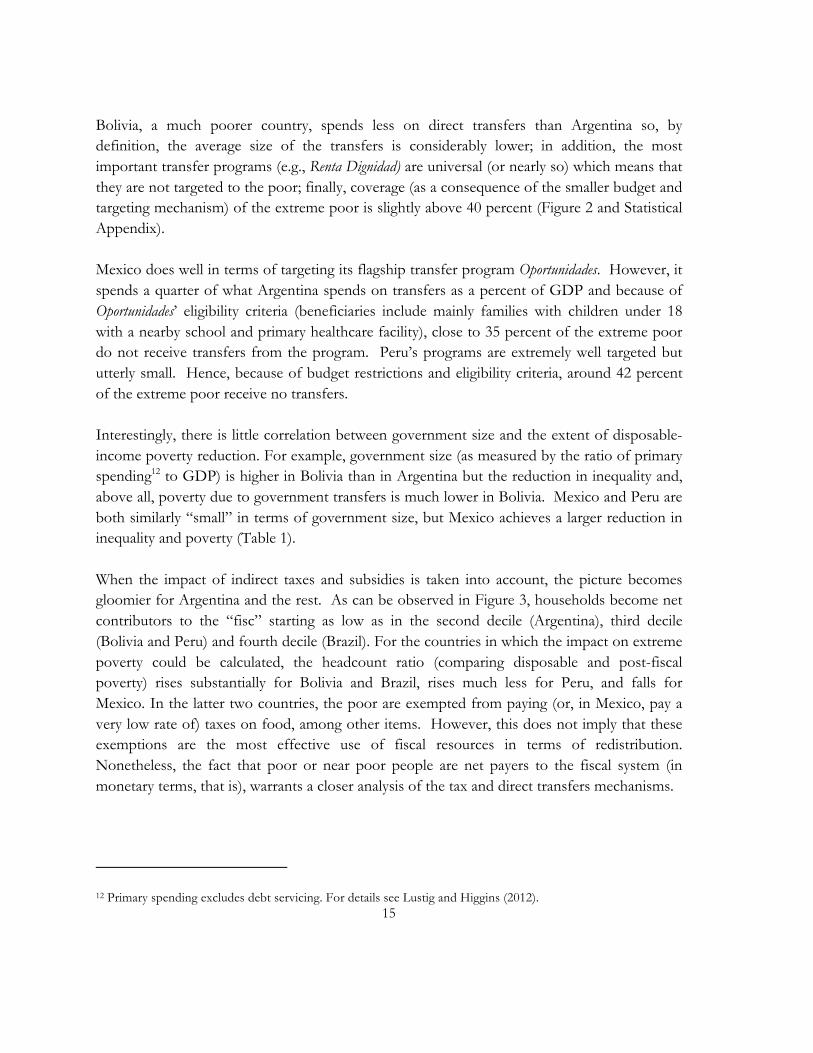
Bolivia, a much poorer country, spends less on direct transfers than Argentina so, by definition, the average size of the transfers is considerably lower; in addition, the most important transfer programs (e.g., Renta Dignidad) are universal (or nearly so) which means that they are not targeted to the poor; finally, coverage (as a consequence of the smaller budget and targeting mechanism) of the extreme poor is slightly above 40 percent (Figure 2 and Statistical Appendix). Mexico does well in terms of targeting its flagship transfer program Oportunidades. However, it spends a quarter of what Argentina spends on transfers as a percent of GDP and because of Oportunidades’ eligibility criteria (beneficiaries include mainly families with children under 18 with a nearby school and primary healthcare facility), close to 35 percent of the extreme poor do not receive transfers from the program. Peru’s programs are extremely well targeted but utterly small. Hence, because of budget restrictions and eligibility criteria, around 42 percent of the extreme poor receive no transfers. Interestingly, there is little correlation between government size and the extent of disposable-income poverty reduction. For example, government size (as measured by the ratio of primary spending12 to GDP) is higher in Bolivia than in Argentina but the reduction in inequality and, above all, poverty due to government transfers is much lower in Bolivia. Mexico and Peru are both similarly “small” in terms of government size, but Mexico achieves a larger reduction in inequality and poverty (Table 1). When the impact of indirect taxes and subsidies is taken into account, the picture becomes gloomier for Argentina and the rest. As can be observed in Figure 3, households become net contributors to the “fisc” starting as low as in the second decile (Argentina), third decile (Bolivia and Peru) and fourth decile (Brazil). For the countries in which the impact on extreme poverty could be calculated, the headcount ratio (comparing disposable and post-fiscal poverty) rises substantially for Bolivia and Brazil, rises much less for Peru, and falls for Mexico. In the latter two countries, the poor are exempted from paying (or, in Mexico, pay a very low rate of) taxes on food, among other items. However, this does not imply that these exemptions are the most effective use of fiscal resources in terms of redistribution. Nonetheless, the fact that poor or near poor people are net payers to the fiscal system (in monetary terms, that is), warrants a closer analysis of the tax and direct transfers mechanisms.

12 Primary spending excludes debt servicing. For details see Lustig and Higgins (2012).

16

Figure 3 – Incidence of Indirect Taxes and Headcount Ratio up to Post-Fiscal Income Incidence of Indirect Taxes

Headcount Ratio

Source: Authors’ calculations based on household surveys and public accounts.

In terms of redistributive effectiveness, Peru and Argentina rank first and second, respectively when assessing the impact of transfers on disposable-income Gini (Table 1). Effectiveness is highest among both the country that redistributes (with direct transfers) the most (Argentina) and the country that redistributes and spends (on transfers) the least (Peru). This means that the effectiveness indicator should be used in conjunction with the magnitude of inequality reduction.

17

ii. Progressiveness of Taxes, Cash Transfers and In-kind Transfers Table 2 presents the distribution of income for each income concept and the concentration shares for each tax and benefit category considered here. As we can see, direct taxes are quite progressive except in Bolivia, a country that does not have personal income taxes. However, the impact of direct taxes on inequality is relatively small because the size of them (with respect to GDP) is about half as much as indirect taxes (see the Statistical Appendix). Indirect taxes are regressive in Argentina, Bolivia and Brazil, practically neutral in Mexico and slightly progressive in Peru. Direct cash transfers are quite progressive in absolute terms in Argentina, Mexico and Peru. In these countries, the bottom (top) quintiles receive 43.0, 38.5 and 49.1 percent (7.6, 14.7 and 2.2 percent) of direct transfers, respectively. In the cases of Bolivia and Brazil, the distribution of cash transfers is pretty flat across deciles; that is, it is progressive only in relative terms (some would say it is neutral in absolute terms). The causes are quite different in both countries, however. In the case of Bolivia, it results from the universalistic nature of the main transfer programs (Renta Dignidad and Juancito Pinto). In the case of Brazil, some of the programs such as Bolsa Familia are very well-targeted to the poor. Others, such as Special Circumstances Pensions benefit relatively more the top quintile. To the extent that it was possible to calculate their incidence, indirect subsidies are regressive in Argentina and Peru and progressive but only in relative terms in Bolivia and Mexico.13 Education spending is progressive in absolute terms in Argentina, Brazil and Peru and to a lesser extent in Mexico and it is flat in the case of Bolivia. Health spending is progressive in absolute terms in Argentina, Brazil and Mexico, and almost flat in Bolivia. (For Peru, the latter could not be calculated with accuracy so it should not be used for comparisons.)

13 In the case of Brazil, the incidence of indirect taxes and subsidies comes from a secondary source and could not be disentangled.

18

Table 2 – Concentration Shares

Notes: a. Note that the above are "concentration shares" by decile. That is, the light grey columns for each definition of income are not the distribution of each income concept that would correspond to the Gini coefficients in Table 1. In the case of Argentina, the "x-axis" of the concentration curve uses households ranked by per capita NET market income; for all the others, households are ranked by market income. In Bolivia, market income and net market income are the same because there are no direct taxes are zero and contributions to social security are negligible. b. For Argentina, the distribution of indirect subsidies and housing and urban were taken from secondary sources that used quintiles; thus deciles could not be used for all transfers or income definitions. c. For Argentina, assuming progressive export taxes.

MarketIncome

DirectTaxesNetMarketIncome

Non‐Contributorypensions

TargetedMonetaryTransfers

OtherDirectTransfers

AllDirectTransfers

DisposableIncome

IndirectSubsidies

IndirectTaxes

NetIndirectTaxes

Post‐FiscalIncome

In‐kindEducation

In‐kindHealth

HousingandUrban

In‐kindTransfers

plusHousing

andUrban

AllTransfers(excludingallTaxes)

AllTransfers(excludingallTaxes)

plusIndirectSubsidies

AllTaxes(DirectandIndirect,incl.

contrib.toSS)c

FinalIncome*

FinalIncome

Argentina

Method:

1 0.7% 0.0% 0.7% 33.7% 18.8% 25.4% 31.6% 2.2% 3.8% 11.9% 18.8% 3.6% 3.6%

(Deciles 2 2.1% 0.0% 2.1% 8.1% 13.6% 26.3% 11.4% 2.6% 4.5% 15.1% 20.5% 4.2% 4.2% 7.7%

orquintiles 3 3.3% 0.0% 3.4% 8.8% 15.3% 15.7% 10.2% 3.7% 5.4% 13.1% 15.4% 5.1% 4.9%

when 4 4.6% 0.0% 4.7% 8.3% 12.0% 11.8% 9.1% 4.9% 6.4% 12.0% 12.7% 6.1% 5.8% 10.6%

decilesnot 5 5.9% 0.0% 6.0% 8.7% 12.9% 8.4% 8.8% 6.2% 7.4% 10.7% 10.4% 7.0% 6.7%

available)b 6 7.5% 0.0% 7.6% 7.8% 11.6% 5.1% 7.5% 7.6% 8.7% 9.8% 7.2% 8.2% 7.8% 14.6%

7 9.7% 0.0% 9.8% 8.1% 4.2% 3.3% 7.1% 9.6% 9.3% 8.4% 5.9% 8.8% 9.5%

8 12.7% 0.2% 12.8% 7.8% 3.9% 2.0% 6.6% 12.5% 12.0% 7.2% 4.6% 11.4% 11.9% 21.3%

9 17.4% 5.7% 17.6% 5.1% 3.5% 1.2% 4.4% 16.9% 15.4% 6.7% 2.9% 14.9% 15.6%

10 36.0% 94.1% 35.3% 3.7% 4.1% 0.8% 3.2% 33.7% 27.1% 5.3% 1.6% 30.6% 30.0% 45.8%

100.0% 100.0% 100.0% 100.0% 100.0% 100.0% 100.0% 100.0% 100.0% 100.0% 100.0% 100.0% 100.0% 100.0% 100.0% 100.0% 100.0% 100.0% 100.0% 100.0% 100.0%

Bolivia

Method:

1 1.3% 10.2% 16.5% 12.6% 11.5% 1.5% 2.4% 3.7% 4.0% 1.4% 10.5% 8.5% 9.7% 9.9% 9.6% 3.7% 2.4% 2.3%

(Deciles) 2 2.6% 8.9% 15.0% 8.1% 9.7% 2.8% 3.7% 4.6% 4.8% 2.7% 10.1% 10.3% 10.1% 10.1% 9.8% 4.6% 3.6% 3.5%

3 3.8% 8.8% 13.3% 15.1% 10.5% 3.9% 5.8% 6.6% 6.8% 3.8% 10.2% 12.9% 11.3% 11.2% 11.0% 6.6% 4.7% 4.7%

4 5.0% 9.5% 13.5% 18.1% 11.5% 5.1% 6.0% 7.5% 7.8% 5.0% 9.7% 10.3% 9.9% 10.2% 10.0% 7.5% 5.6% 5.6%

5 6.2% 8.4% 10.9% 12.9% 9.5% 6.2% 7.9% 7.3% 7.2% 6.2% 10.3% 11.3% 10.7% 10.6% 10.5% 7.3% 6.7% 6.7%

6 7.7% 9.1% 9.8% 13.2% 9.9% 7.8% 10.8% 9.3% 9.0% 7.7% 10.2% 10.5% 10.3% 10.3% 10.3% 9.3% 8.0% 8.0%

7 9.4% 8.9% 8.1% 5.3% 8.2% 9.3% 8.9% 9.8% 10.0% 9.3% 10.9% 10.3% 10.6% 10.3% 10.2% 9.8% 9.5% 9.5%

8 11.8% 11.7% 6.0% 4.7% 9.6% 11.7% 12.4% 12.3% 12.3% 11.7% 10.8% 8.6% 9.9% 9.8% 10.0% 12.3% 11.5% 11.5%

9 16.3% 10.1% 4.6% 8.0% 8.9% 16.2% 14.5% 15.1% 15.3% 16.2% 10.2% 8.7% 9.6% 9.5% 9.7% 15.1% 15.5% 15.5%

10 36.0% 14.5% 2.3% 2.0% 10.6% 35.5% 27.6% 23.6% 22.8% 35.9% 7.2% 8.6% 7.8% 8.2% 9.0% 23.6% 32.4% 32.7%

100.0% 100.0% 100.0% 100.0% 100.0% 100.0% 100.0% 100.0% 100.0% 100.0% 100.0% 100.0% 100.0% 100.0% 100.0% 100.0% 100.0% 100.0%

Brazil

Method:

1 0.8% 0.0% 0.8% 30.1% 34.3% 7.2% 13.1% 1.5% 1.4% 1.4% 1.6% 15.5% 11.2% 13.5% 13.4% 13.4% 1.2% 3.0% 3.2%

(Deciles) 2 1.7% 0.2% 1.8% 18.5% 25.4% 5.6% 9.4% 2.3% 2.1% 2.1% 2.3% 13.4% 11.9% 12.7% 11.6% 11.6% 1.7% 3.5% 3.7%

3 2.7% 0.4% 2.7% 14.7% 17.0% 6.6% 8.7% 3.1% 2.9% 2.9% 3.2% 12.1% 12.0% 12.1% 11.0% 11.0% 2.4% 4.2% 4.4%

4 3.6% 0.8% 3.8% 13.2% 10.5% 7.5% 8.5% 4.0% 3.8% 3.8% 4.1% 10.9% 12.2% 11.5% 10.6% 10.6% 3.2% 4.9% 5.1%

5 4.8% 1.2% 4.9% 8.5% 6.0% 9.9% 9.3% 5.2% 5.0% 5.0% 5.3% 9.4% 11.6% 10.5% 10.1% 10.1% 4.2% 5.8% 6.0%

6 6.2% 1.7% 6.4% 7.4% 3.0% 9.7% 8.7% 6.5% 6.4% 6.4% 6.6% 8.9% 11.4% 10.1% 9.6% 9.6% 5.5% 7.0% 7.1%

7 8.1% 2.5% 8.3% 2.8% 1.7% 10.4% 8.5% 8.3% 8.1% 8.1% 8.4% 8.0% 10.7% 9.3% 9.0% 9.0% 7.0% 8.5% 8.5%

8 11.0% 4.8% 11.2% 2.1% 1.0% 10.9% 8.7% 11.1% 11.0% 11.0% 11.1% 7.8% 8.9% 8.3% 8.4% 8.4% 9.7% 10.7% 10.7%

9 16.3% 10.3% 16.5% 1.6% 0.6% 10.7% 8.4% 16.0% 16.2% 16.2% 16.0% 6.6% 7.0% 6.8% 7.3% 7.3% 14.9% 14.9% 14.7%

10 44.9% 77.9% 43.5% 1.2% 0.3% 21.5% 16.6% 41.9% 43.0% 43.0% 41.6% 7.3% 3.1% 5.3% 8.8% 8.8% 50.1% 37.5% 36.6%

100.0% 100.0% 100.0% 100.0% 100.0% 100.0% 100.0% 100.0% 100.0% 100.0% 100.0% 100.0% 100.0% 100.0% 100.0% 100.0% 100.0% 100.0% 100.0%

Mexico

Method:

1 1.0% 0.3% 1.1% 17.7% 34.0% 14.3% 23.9% 1.3% 3.6% 1.1% ‐3.4% 1.4% 11.5% 10.4% 11.1% 12.3% 10.0% 0.7% 2.3% 2.4%

(Deciles) 2 2.2% 0.7% 2.3% 10.7% 22.0% 7.5% 14.6% 2.5% 4.9% 2.2% ‐2.6% 2.6% 11.3% 9.8% 10.8% 11.1% 9.5% 1.5% 3.3% 3.4%

3 3.3% 1.0% 3.4% 10.1% 15.4% 6.9% 11.2% 3.5% 6.2% 3.3% ‐1.9% 3.6% 11.2% 9.7% 10.7% 10.7% 9.5% 2.1% 4.2% 4.3%

4 4.3% 1.3% 4.4% 9.2% 11.0% 8.6% 9.8% 4.5% 7.7% 4.5% ‐1.3% 4.6% 11.2% 9.7% 10.7% 10.6% 9.8% 2.8% 5.1% 5.2%

5 5.4% 1.7% 5.6% 8.1% 6.5% 9.3% 7.8% 5.6% 8.4% 5.8% 1.0% 5.7% 10.4% 9.6% 10.1% 9.9% 9.5% 3.6% 6.1% 6.2%

6 6.8% 2.8% 7.0% 8.4% 5.4% 8.2% 6.9% 7.0% 9.7% 6.8% 1.4% 7.1% 10.1% 10.0% 10.1% 9.8% 9.8% 4.5% 7.3% 7.4%

7 8.5% 5.1% 8.7% 8.7% 2.6% 9.7% 6.3% 8.7% 11.0% 9.0% 5.3% 8.8% 9.7% 10.1% 9.8% 9.5% 9.9% 6.7% 8.8% 8.9%

8 11.2% 8.9% 11.3% 9.0% 1.9% 6.5% 4.8% 11.3% 12.3% 11.7% 10.5% 11.3% 9.3% 10.3% 9.6% 9.2% 10.0% 10.0% 11.1% 11.1%

9 16.2% 17.9% 16.1% 8.3% 0.7% 7.9% 4.6% 16.0% 14.6% 17.2% 22.1% 15.9% 8.6% 10.6% 9.3% 8.9% 10.4% 17.4% 15.3% 15.2%

10 41.0% 60.2% 40.0% 9.9% 0.6% 21.1% 10.0% 39.7% 21.6% 38.4% 68.9% 39.0% 6.8% 9.9% 7.9% 8.1% 11.6% 50.7% 36.6% 35.9%

100.0% 100.0% 100.0% 100.0% 100.0% 100.0% 100.0% 100.0% 100.0% 100.0% 100.0% 100.0% 100.0% 100.0% 100.0% 100.0% 100.0% 100.0% 100.0% 100.0%

Perud

Method:

1 1.2% 0.0% 1.2% 41.2% 23.1% 29.4% 1.3% 0.4% 0.4% 0.4% 1.4% 13.8% 1.5% 9.2% 11.2% 8.8% 0.4% 1.7% 1.7%

(Deciles) 2 2.3% 0.0% 2.4% 25.1% 16.7% 19.7% 2.4% 1.2% 0.9% 0.8% 2.5% 12.9% 1.8% 8.8% 9.9% 8.0% 0.7% 2.7% 2.8%

3 3.4% 0.0% 3.4% 16.4% 16.3% 16.3% 3.5% 2.2% 2.0% 1.9% 3.6% 12.8% 2.4% 9.0% 9.7% 8.0% 1.6% 3.7% 3.8%

4 4.5% 0.0% 4.5% 8.1% 12.9% 11.2% 4.6% 3.1% 3.1% 3.1% 4.7% 12.1% 3.9% 9.1% 9.3% 7.9% 2.5% 4.8% 4.9%

5 5.8% 0.0% 5.8% 4.9% 9.8% 8.1% 5.8% 3.7% 4.3% 4.5% 5.9% 11.3% 6.5% 9.5% 9.4% 8.1% 3.5% 6.0% 6.1%

6 7.3% 0.3% 7.4% 1.8% 7.2% 5.3% 7.4% 5.4% 6.4% 6.7% 7.4% 9.8% 5.9% 8.3% 8.0% 7.5% 5.3% 7.4% 7.5%

7 9.2% 0.9% 9.3% 1.2% 5.1% 3.7% 9.3% 8.1% 9.0% 9.3% 9.3% 8.4% 9.7% 8.8% 8.3% 8.3% 7.6% 9.3% 9.3%

8 11.8% 1.4% 12.0% 0.6% 5.9% 4.1% 11.9% 8.6% 11.1% 11.7% 12.0% 8.3% 16.0% 11.1% 10.4% 10.0% 9.3% 11.9% 11.9%

9 16.3% 5.7% 16.4% 0.6% 1.9% 1.5% 16.4% 17.2% 18.0% 18.2% 16.3% 6.7% 19.9% 11.6% 10.6% 12.1% 15.8% 16.2% 16.1%

10 38.3% 91.7% 37.5% 0.1% 1.1% 0.7% 37.4% 50.1% 44.7% 43.4% 37.0% 4.0% 32.4% 14.5% 13.2% 21.2% 53.2% 36.4% 36.1%

100.0% 100.0% 100.0% 100.0% 100.0% 100.0% 100.0% 100.0% 100.0% 100.0% 100.0% 100.0% 100.0% 100.0% 100.0% 100.0% 100.0% 100.0% 100.0%

ImputationMethod

ImputationMethod

DirectIdentification



ImputationMethod

ImputationMethod

ImputationMethod


SecondarySources


DirectIDandAltSurvey

ImputationandAltSurvey

ImputationandAltSurvey

SecondarySources

ImputationMethod





SecondarySources

ImputationMethod

AlternateSurvey


SimulationMethod

DirectIDandSimulation

ImputationMethod

SecondarySources

ImputationMethod

SecondarySources

InferenceMethod


SimulationMethod

SecondarySources

SecondarySources

ImputationMethod

Total

Total

Total

Total

Total

16.8%

40.2% 44.3% 51.6% 23.5% 12.6% 11.4% 20.0%

20.7% 21.7% 22.2% 21.4% 15.6% 15.2%

20.1%

18.5% 14.3% 13.7% 19.9% 19.6% 18.8% 18.7%

12.9% 11.1% 8.3% 18.2% 24.3% 23.1%

7.8% 8.6% 4.2% 17.0% 27.8% 31.4% 24.4%

ImputationMethod

SecondarySources

19

d. Peru not comparable with other countries because health spending includes only a fraction of public spending on health due to data limitations.

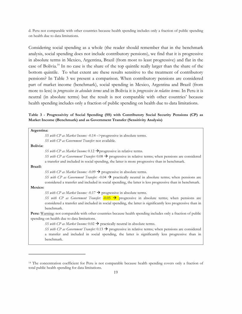
Considering social spending as a whole (the reader should remember that in the benchmark analysis, social spending does not include contributory pensions), we find that it is progressive in absolute terms in Mexico, Argentina, Brazil (from most to least progressive) and flat in the case of Bolivia.14 In no case is the share of the top quintile really larger than the share of the bottom quintile. To what extent are these results sensitive to the treatment of contributory pensions? In Table 3 we present a comparison. When contributory pensions are considered part of market income (benchmark), social spending in Mexico, Argentina and Brazil (from more to less) is progressive in absolute terms and in Bolivia it is progressive in relative terms. In Peru it is neutral (in absolute terms) but the result is not comparable with other countries’ because health spending includes only a fraction of public spending on health due to data limitations. Table 3 - Progressivity of Social Spending (SS) with Contributory Social Security Pensions (CP) as Market Income (Benchmark) and as Government Transfer (Sensitivity Analysis)

Argentina: SS with CP as Market Income: -0.14 –>progressive in absolute terms. SS with CP as Government Transfer: not available.

Bolivia: SS with CP as Market Income: 0.12 progressive in relative terms. SS with CP as Government Transfer: 0.08 progressive in relative terms; when pensions are considered a transfer and included in social spending, the latter is more progressive than in benchmark.

Brazil: SS with CP as Market Income: -0.09 progressive in absolute terms. SS with CP as Government Transfer: -0.04 practically neutral in absolute terms; when pensions are considered a transfer and included in social spending, the latter is less progressive than in benchmark.

Mexico: SS with CP as Market Income: -0.17 progressive in absolute terms. SS with CP as Government Transfer: -0.05 progressive in absolute terms; when pensions are considered a transfer and included in social spending, the latter is significantly less progressive than in benchmark.

Peru: Warning: not comparable with other countries because health spending includes only a fraction of public spending on health due to data limitations.

SS with CP as Market Income: 0.02 practically neutral in absolute terms. SS with CP as Government Transfer: 0.13 progressive in relative terms; when pensions are considered a transfer and included in social spending, the latter is significantly less progressive than in benchmark.

14 The concentration coefficient for Peru is not comparable because health spending covers only a fraction of total public health spending for data limitations.

20

Notes: When contributory social security pensions are classified as government transfers, social spending includes contributory pensions and so does the corresponding concentration coefficient. “Neutral in absolute terms” means that per capita transfers are the same for everyone.

Interestingly, when contributory pensions are included under government transfers (our sensitivity analysis), whether social spending plus contributory pensions becomes more or less progressive varies by country. In Bolivia, it becomes more progressive while in Brazil, Mexico and Peru it becomes less progressive. The changes are particularly striking for Mexico – where the concentration coefficient increases by 12 percentage points– and Peru – where the concentration coefficient increases by 11 percentage points and social spending switches from neutral (per capita social spending is the same across income levels) to progressive in relative terms (per capita social spending increases with income but as a share of market income it declines).

4. CONCLUDING REMARKS Standard tax and benefits incidence analysis reveals that the extent of inequality reduction induced by direct taxes and (mainly cash) transfers in Argentina, Bolivia, Brazil, Mexico and Peru is rather small when compared with that found in advanced countries. In our five-country sample, the Gini declines by 2 percentage points on average whereas in fifteen Western European countries the Gini declined by 15 percentage points (Goñi et al. 2011; Table 1). Compared to Goñi et al. (2011; Table 1) 15, however, the results found in our study show more income inequality reduction for Argentina (Gini declines by 3 percentage points in our analysis and 1 percentage point in theirs) and Brazil (Gini declines by 5 percentage points in our analysis and 3 percentage points in theirs). 16 At this point it is difficult to say how much these differences are due to a change in these countries’ policies (Goñi et al. use information from earlier years than our study) or differences in methodology (Goñi et al. rely on secondary sources). While in Mexico and Peru the limited extent of cash transfers-based redistribution could arguably be attributed to the relatively small size of the “fiscal pie,” that is not the case of Argentina, Bolivia and Brazil. In the latter three countries, primary spending as a percent of GDP is 38, 45 and 37 percent, respectively, close to the ratio found in advanced countries. What prevents these countries from achieving similar cash transfers-based reductions in inequality is not the lack of revenues. The reason is a combination of two factors. First,

15 The results we compare here are for our sensitivity analysis (contributory pensions as government transfers) available upon request because Goñi et al., op. cit., include social insurance pensions under government transfers. 16 For Mexico and Peru the results are practically the same in both studies. When transfers in-kind are included, the differences become more striking for all five countries. Goñi et al., op. cit., does not include Bolivia.

21

Argentina, Bolivia and Brazil still spend less on cash transfers as a share of GDP than advanced countries, with Bolivia (Brazil) spending the least (most) of the three.17 Second, the share that Bolivia and Brazil spend on direct transfers that are progressive in absolute terms is not large enough. As one can observe in Table 2, in Bolivia and Brazil the concentration shares of direct cash transfers are practically flat (that is, similar across deciles). In the case of Bolivia, even the distribution of the so-called targeted cash transfers is flat; as we saw above, the flagship cash transfers (e.g., Juancito Pinto and Renta Dignidad ) exclude about 60 percent of the poor and give 60 percent of the benefits to the nonpoor. In the case of Brazil, the flagship Bolsa Familia and BPC are well targeted to the poor but exclude about a third of them from transfers; moreover, the largest cash transfer (as a percent of GDP), the Special Circumstances Pension, is not progressive in absolute terms (only in relative terms). It turns out that Mexico and Peru, although they are definitely more fiscally constrained –and by far-- than the other three countries, also spend relatively little on direct cash transfers as a proportion of primary spending and, in the case of Mexico, the share spent on transfers that are progressive in absolute terms is relatively small giving the same result we found for Bolivia and Brazil: the concentration shares of direct cash transfers are practically flat across deciles (Table 3). When we add the effect of indirect taxes and subsidies and compare the Gini for post-fiscal income with the disposable income Gini, net indirect taxes are unequalizing for Argentina and Bolivia and equalizing for Brazil, Mexico and Peru. Indirect taxes are outright regressive in Argentina, Bolivia and Brazil and practically neutral in Mexico and slightly progressive in Peru. As discussed in the previous section, households become net contributors to the “fisc” on average starting as low as in the second decile (Argentina), third decile (Bolivia and Peru) and fourth decile (Brazil). The post-fiscal headcount ratio for extreme poverty (compared with disposable-income poverty) rises substantially for Bolivia and Brazil, rises much less for Peru, and falls for Mexico.18 In the latter two countries, the poor are exempted from paying (or, in Mexico, pay a very low rate of) VAT on food.19 Care must be taken to conclude from this that indirect taxes should be lowered or exemptions should be kept. Revenues collected in the form of indirect taxes in Argentina, Bolivia and Brazil, for example, may be going back to the lower deciles in the form of in-kind transfers in, for example, education and health. However, the fact that in monetary terms some of the poor and near poor households become net contributors to the government coffers is not a welcome result. It warrants an analysis of the

17 Remember that these direct cash transfers in our benchmark analysis do not include contributory pensions. So, they are primarily noncontributory schemes. 18 This indicator could not be calculated for Argentina. 19 In fact, Lustig and Higgins (2012) show that indirect taxes cause 4 percent of the extreme poor to become ultra-poor and 15 percent of the moderate poor to become extreme poor.

22

tax and cash benefits system as a whole to identify ways in which the poor could be prevented from being net payers in monetary terms.20 To what extent are the regressive revenues in indirect taxes returned to the bottom fifty percent of the population in the form of in-kind transfers? When indirect subsidies and –above all-- transfers in-kind are added, the poorest six deciles are net receivers of fiscal resources in all five countries.21 Thus, one could argue that what the state takes away in indirect taxes, the state gives back in education and health spending. However, while this is true, we also know that all five countries seem to have fiscal space to make cash transfers more redistributive. First, the share allocated to direct cash transfers could be increased. Second, the share allocated to cash transfers progressive in absolute terms could be increased. Third, direct cash transfers could be designed in such a way to cover as close as possible the universe of the extreme poor.22

20 When contributory pensions are classified as a government transfer, although social spending plus pensions becomes less progressive in Brazil, Mexico and Peru (in Bolivia it becomes more progressive) the net contributors to the fiscal system start at higher deciles. This is not surprising. Under this scenario, the market income poor include all the pensioners whose before pensions income is close to zero. Pensions as transfers increase their disposable income by a large proportion and hence the negative effect of indirect taxes on their income (post-fiscal income) is more than compensated. 21 See incidence table in Statistical Appendix (available upon request). 22 In addition, although in-kind transfers in education have a flat distribution, this is not the case for, for example, upper secondary and tertiary education. (Concentration shares of public spending on education by level are available upon request.) There is still ample room for equalizing opportunities by increasing the access to tertiary education among the young in the lowest deciles (not to mention increasing the access to education of better quality at all levels).

23

REFERENCES Barnard, Andrew. 2009. “The effects of taxes and benefits on household income, 2007/08.”

Economic & Labour Market Review 3(8): 56-66. Birdsall, Nancy, Augusto de la Torre, and Rachel Menezes. 2008. Fair Growth. Washington,

D.C.: Center for Global Development and Inter-American Dialogue. Breceda, Karla, Jamele Rigolini, and Jaime Saavedra. 2008. “Latin America and the Social

Contract: Patterns of Social Spending and Taxation.” Policy Research Working Paper 4604, Washington, D.C.: The World Bank.

Ferreira, Francisco H. G., and Martin Ravallion. 2008. “Global Poverty and Inequality : a Review of the Evidence.” Policy Research Working Paper 4623, Washington, D.C.: The World Bank.

Goñi, Edwin, J. Humberto López, and Luis Servén. 2011. “Fiscal Redistribution and Income Inequality in Latin America.” World Development 39(9): 1558-1569.

Immervoll, Herwig, Horacio Levy, José Ricardo Nogueira, Cathal O’Donoghue, and Rozane Bezerra de Siqueira. 2009. “The Impact of Brazil’s Tax-Benefit System on Inequality and Poverty.” Poverty, Inequality, and Policy in Latin America. Eds. Stephan Klasen, and Felicitas Nowak-Lehmann. Cambridge: Mass.: MIT Press. 271-302.

Inter-American Development Bank. 2011. Social Strategy for Equity and Productivity. Latin America and the Caribbean. Washington, D.C.: IDB.

Kakwani, Nanak C. 1977. “Measurement of Tax Progressivity: An International Comparison.” The Economic Journal 87(345): 71-80.

Lambert, Peter. 1985. “On the redistributive effect of taxes and benefits.” Scottish Journal of Political Economy 32(1): 39-54.

Lindert, Kathy, Emmanuel Skoufias, and Joseph Shapiro. 2006. “Redistributing Income to the Poor and Rich: Public Transfers in Latin America and the Caribbean.” Social Protection Discussion Paper 0605. Washington, D.C.: The World Bank.

Lustig, Nora and Sean Higgins. 2012. “Commitment to Equity Assessment (CEQ): A Diagnostic Framework to Assess Governments’ Fiscal Policies Handbook,” Tulane

Economics Department and CIPR, Working Paper, New Orleans, Louisiana. ________________________ . 2012. “Fiscal Incidence, Fiscal Mobility and the Poor: A New

Approach.” Tulane University Economics Working Paper 1202. O’Donnell, Owen, Eddy van Doorslaer, Adam Wagstaff, and Magnus Lindelow. 2008.

Analyzing Health Equity Using Household Survey Data: A Guide to Techniques and Their Implementation. Washington, D.C.: The World Bank.

Scott, John. 2011. “Gasto Público y Desarrollo Humano en México: Análisis de Incidencia y Equidad.” Working Paper for Informe sobre Desarrollo Humano México 2011. Mexico City: UNDP.

24

Silveira, Fernando Gaiger, Jhonatan Ferreira, Joana Mostafa and José Aparecido Carlos Ribeiro. 2011. “Qual o Impacto da Tributação e dos Gastos Públicos Sociais na Distribuição de Renda do Brasil? Observando os Dois Lados da Moeda.” Progressividade da Tributação e Desoneração da Folha de Pagamentos Elementos para Reflexão. Eds. José Aparecido Carlos Ribeiro, Álvaro Luchiezi Jr., and Sérgio Eduardo Arbulu Mendonça. Brasilia: IPEA. 25-63.

25

APPENDIX: INCOME CONCEPTS DEFINITIONS

Market income is defined as: Im = W + IC + AC + IROH + PT + SSP Where,

Im = market income23 W = gross (pre-tax) wages and salaries in formal and informal sector; also known as earned income. IC = income from capital (dividends, interest, profits, rents, etc.) in formal and informal sector; excludes capital gains and gifts. AC = autoconsumption; also known as self-production.24 IROH = imputed rent for owner occupied housing; also known as income from owner occupied housing. PT = private transfers (remittances and other private transfers such as alimony). SSP = retirement pensions from contributory social security system.

Net Market income is defined as:

In = Im – DT – SSC

Where, In = net market income. DT = direct taxes on all income sources (included in market income) that are subject to taxation. SSC = all contributions to social security except portion going towards pensions.25

Disposable income is defined as:

Id = In + GT Where,

Id = disposable income.

23 Market income is sometimes called primary income. 24 This item is included it whenever reported by surveys. 25 Since here we are treating contributory pensions as part of market income, the portion of the contributions to social security going towards pensions are treated as ‘saving.’

26

GT = direct government transfers; mainly cash but can include transfers in kind such as food.

Post-fiscal income is defined as: Ipf = Id + IndS – IndT Where, Ipf = post-fiscal income. IndS = indirect subsidies. IndT = indirect taxes (e.g., value added tax or VAT, sales tax, etc.). Final income is defined as: If = Ipf + InkindT – CoPaym (benchmark) Where, If = final income.

InkindT = government transfers in the form of free or subsidized services in education and health; urban and housing. CoPaym = co-payments, user fees, etc., for government services in education and health.26

Because some countries do not have data on indirect subsidies and taxes, we also

defined Final income* = If* = Id + InkindT – CoPaym.

The definitions are summarized in Diagram 1. For a detailed description of how each income concept was constructed in the five countries see Appendix A of the Statistical Appendix.

26 One may also include participation costs such as transportation costs or foregone incomes because of use of time in obtaining benefits. In our study, they were not included.

29

CEQ WORKING PAPER SERIES

“Commitment to Equity Assessment (CEQ): Estimating the Incidence of Social Spending,

Subsidies and Taxes. Handbook,” by Nora Lustig and Sean Higgins, CEQ Working Paper No. 1, July 2011; revised January 2013.

“Commitment to Equity: Diagnostic Questionnaire,” by Nora Lustig, CEQ Working Paper No. 2, 2010; revised August 2012.

“The Impact of Taxes and Social Spending on Inequality and Poverty in Argentina, Bolivia, Brazil, Mexico and Peru: A Synthesis of Results,” by Nora Lustig, George Gray Molina, Sean Higgins, Miguel Jaramillo, Wilson Jiménez, Veronica Paz, Claudiney Pereira, Carola Pessino, John Scott, and Ernesto Yañez, CEQ Working Paper No. 3. August 2012.

“Fiscal Incidence, Fiscal Mobility and the Poor: A New Approach,” by Nora Lustig and Sean Higgins, CEQ Working Paper No. 4, September 2012.

“Social Spending and Income in Argentina in the 2000s: the Rising Role of Noncontributory Pensions,” by Nora Lustig and Carola Pessino, CEQ Technical Paper No. 5, January 2013. “Explaining Low Redistributive Impact in Bolivia,” by Verónica Paz Arauco, George Gray Molina, Wilson Jiménez Pozo, and Ernesto Yáñez Aguilar, CEQ Working Paper No. 6, January 2013.

“The Effects of Brazil’s High Taxation and Social Spending on the Distribution of Household Income,” by Sean Higgins and Claudiney Pereira, CEQ Working Paper No. 7, January 2013. “Redistributive Impact and Efficiency of Mexico’s Fiscal System,” by John Scott, CEQ Working Paper No. 8, January 2013.

“The Incidence of Social Spending and Taxes in Peru,” by Miguel Jaramillo Baanante, CEQ Working Paper No. 9, January 2013.

“Social Spending, Taxes, and Income Redistribution in Uruguay,” by Marisa Bucheli, Nora Lustig, Máximo Rossi and Florencia Amábile, CEQ Working Paper No. 10, January 2013.

“Social Spending, Taxes and Income Redistribution in Paraguay,” Sean Higgins, Nora Lustig, Julio Ramirez (CADEP), Billy Swanson, CEQ Working Paper No. 11, February 2013.

30

The CEQ logo is a stylized graphical representation of a Lorenz curve for a fairly unequal distribution of income (the bottom part of the C, below the diagonal) and a concentration curve for a very progressive transfer (the top part of the C).

What is CEQ?

Led by Nora Lustig (Tulane University) and Peter Hakim (Inter-American Dialogue), the Commitment to Equity (CEQ) project is designed to analyze the impact of taxes and social spending on inequality and poverty, and to provide a roadmap for governments, multilateral institutions, and nongovernmental organizations in their efforts to build more equitable societies. CEQ/Latin America is a joint project of the Inter-American Dialogue (IAD) and Tulane University’s Center for Inter-American Policy and Research (CIPR) and Department of Economics. The project has received financial support from the Canadian International Development Agency (CIDA), the Development Bank of Latin America (CAF), the General Electric Foundation, the Inter-American Development Bank (IADB), the International Fund for Agricultural Development (IFAD), the Norwegian Ministry of Foreign Affairs, the United Nations Development Programme’s Regional Bureau for Latin America and the Caribbean (UNDP/RBLAC), and the World Bank. http://commitmenttoequity.org

THE IMPACT OF TAXES AND SOCIAL SPENDING ON...

Documents

Transcript of THE IMPACT OF TAXES AND SOCIAL SPENDING ON...