The Impact of Tax Exclusive and Inclusive Prices on...

The Impact of Tax Exclusive and Inclusive Prices onDemand∗

Naomi E. FeldmanResearch Division

Federal Reserve BoardWashington, D.C. 20551

[email protected]

Bradley J. RuffleDepartment of Economics

Ben-Gurion UniversityBeer Sheva, Israel

[email protected]

January 2012

Preliminary Draft

Abstract: Whether the sales tax is included in the price or added on at the cash register ought notaffect purchases of the rational consumer. We test this tax-equivalence hypothesis with a number ofexperimental treatments that differ only in their handling of the tax. Subjects are given a cash budgetfrom which they decide how much to keep and how much to spend on various attractively priced goods.Subjects repeat this allocation task over ten rounds with the selection of goods and their prices varyingbetween rounds. We find that subjects spend significantly more when faced with tax-exclusive priceswhere the tax is added on at the register compared to tax-inclusive prices. Results from an additionaltreatment in which the sales tax is deducted at the cash register reveal that neither salience nor anoptimism bias can account for our treatment effect.

JEL codes: C91, H20, H31.

Keywords: experimental economics, sales tax, VAT, tax salience.

∗We thank Leif Danziger, Eyal Ert and Ro’i Zultan for valuable comments and seminar participants from Ben-Gurion Uni-versity, the Federal Reserve Board, the 4th Psychology of Investment Conference and the University of Michigan. Ziv Ben-Naimprovided excellent research assistance. We are grateful to Ben-Gurion University for funding the experiments. The analysisand conclusions set forth are those of the authors and do not indicate concurrence by other members of the research staff or theBoard of Governors. All errors are our own.

1

1 Introduction

A growing economics literature challenges the view that economic actors duly weigh all of the

relevant features of a decision problem in making choices. Following Morwitz, Greenleaf and Johnson’s

(1998) early work on price partitioning, a series of recent papers (see, for example, Chetty et al. (2009),

Hossain and Morgan (2006), Brown, Hossain and Morgan (2010)) show that some components of a

price are less prominent than others and this impacts individual behavior. In this paper, we test the

equivalence of tax-inclusive and tax-exclusive prices in a controlled laboratory experiment. We present

each subject with a series of attractive goods that are highly discounted in price and an endowment

to spend or to keep as each sees fit. Each subject repeats this task over ten rounds with the selection

of products and their prices varying across rounds. In a between-subject design, subjects are informed

that all prices include VAT (tax-inclusive treatment or TI), or, that the tax will be added to all prices

at the checkout (tax-exclusive treatment or TE).1 Our experimental design thus provides us with

individual-level purchasing decisions under varied conditions that are systematically controlled by the

experimenters.

The previous empirical literature has found that shrouding or making less “salient” certain ele-

ments of a total price results in larger purchases than would be made if the full price were clearly

presented. It follows that one potential way to increase demand is for retailers to separate their total

prices into upfront fees and less visible taxes, service fees and other surcharges.2 On the other hand,

such a conclusion may be premature because existing studies tell us little about the role of informa-

tion and how individuals respond when faced repeatedly with these pricing schemes. It is certainly

possible that individuals learn over the medium or longer term to internalize the tax to be added on at

the register or the separate shipping and handling charges. Our study also investigates learning in a

simpler, mostly static, repeated environment. If individuals fail to learn to internalize the tax in our

setup, then arguably they will not succeed in doing so in a more complex, dynamic environment.

An alternative to the salience explanation is what we refer to as an “optimism” bias. Accordingly,

individuals use simplifying heuristics to compute tax-inclusive prices that systematically underesti-

mate costs and overestimate rewards. To illustrate, when contemplating the purchase of a good with1Our experiment was run in Israel where the VAT is 16%.2Industries in which prices are commonly broken down by price component include banking, mutual funds and online re-

tailers. With fees for checked baggage, meals, early boarding, flight changes, high fuel costs and, most recently, advance seatassignment, the airlines employ the widest and most creative range of price components. The Bureau of Transportation Statis-tics estimates that fees from checked baggage and reservation changes alone accounted for 4% of airline operating revenue and62% of operating profit in the second quarter of 2011 (McCartney 2011).

2

a tax-exclusive price, an individual may be fully aware of the existence of the tax and even the precise

tax rate. Yet, the individual underestimates the magnitude of the tax to be paid in order to reduce

the cognitive dissonance associated with purchasing at a higher price. This underestimation of the

final tax-inclusive price leads to higher consumption. The flip side of this bias is that individuals

overestimate discounts in order to feel psychological satisfaction from paying a lower price.

To evaluate salience and the optimism bias, we introduce a third, tax-deduction (TD) treatment.

Subjects in TD are informed that the prices of the goods include VAT and that the tax will be refunded

at the checkout. The pre-deduction prices are set such that the final prices of goods in TD are iden-

tical to those in TE and TI to facilitate a clean comparison of purchasing behavior between the three

treatments. To the best of our knowledge, the previous literature on salience addresses the effect of

shrouding only for positive price components of the total price (like a tax or shipping and handling

fee). The impact on demand of shrouding a negative price component of the total price (such as a VAT

refund or other percentage discount) has not been explored. Based upon the current state of knowledge

of the role of salience, one would expect the effect of salience to be symmetric for positive and negative

price components; that is, just as individuals overconsume when approaching the tax-inclusive price

from below, salience would predict that they underconsume when approaching the tax-inclusive price

from above. The optimism bias, by contrast, predicts overconsumption in both cases relative to the

tax-inclusive case because taxes are underestimated and discounts are overestimated.3

This paper addresses the above issues. First, we test whether consumption patterns differ between

subjects facing tax-exclusive prices and those facing tax-inclusive prices. Our experimental design

permits us to evaluate how any observed differences in consumption respond to learning (over the

ten rounds) and how they vary by price level, type of good and/or elasticity. Moreover, a third, tax-

deduction treatment allows us assess the validity of the salience explanation that other studies have

offered versus an optimism bias.

We find that subjects facing the tax-exclusive treatment spend, on average, 5.7 New Israeli Shekels

(or $1.58 USD) more (roughly 30%) than those subjects facing the full tax-inclusive price. Moreover,

while the effect shows signs of weakening in the latter rounds, the treatment difference remains sta-

tistically significant at conventional levels. This result suggests that subjects do not fully incorporate

the tax even when faced with ten rounds of nearly identical purchasing decisions. Additionally, we3 The magnitudes of the effects are case dependent because how much individuals underestimate costs or overestimate

benefits is ad-hoc and not necessarily symmetric. A 16% sales tax may be mentally computed using 10% as a rough estimate toadd onto the price but in the case of a 16% price discount, 20% may be used as the rough estimate to subtract from the price.

3

find that the effect is good dependent, stronger when the price level is higher and, as expected, when

elasticities are higher in absolute value.

Finally, in a separate analysis, we estimate the amount of the tax that is internalized. We find

that that subjects internalize approximately .054 out of .16 or, one-third of the tax on average over the

ten goods. Individually, the point estimates of the ten goods used in our experiment range from zero

(completely ignoring the tax) to near full internalization at .138 or 85% of the tax. However, in the

majority of the cases, we do not reject at standard levels of significance that the entire tax is ignored.

The next section reviews the related literature. Section 3 details the experimental design and

procedures. The results of the TE and TI treatments are presented in section 4 and analyzed by

various subgroups. In section 5, we estimate the amount of the tax internalized for each good in the

TE treatment. Section 6 introduces a third TD treatment designed to assess whether salience or

optimism can account for our observed treatment effect. Learning and the persistence of treatment

differences over time are evaluated in section 7. Section 8 summarizes the main findings and offers

some policy implications.

2 Literature

The most closely related paper to ours is Chetty, Looney and Kraft (2009). They conduct a natural

field experiment in a grocery store to compare purchases under tax-exclusive and tax-inclusive prices.

Price tags display original pre-tax prices, the amount of the sales tax and the final tax-inclusive price

for a subset of three products groups. Scanner data show that their intervention reduced demand for

the treated products by about 8% on average compared to two control groups: other products in same

aisle and similar products sold in two nearby grocery stores.

A particular concern in Chetty et al. (2009) is the unnaturalness of tax-inclusive pricing in the

United States or what they call “Hawthorne” effects. The large, unusual tax-inclusive tags may have

deterred suspicious consumers from purchasing the treated goods. Moreover, these Hawthorne effects

are present only for the tax-inclusive goods and not for the control goods. This could ultimately explain

why individuals purchased less.4

To the extent that Hawthorne effects are relevant in our (or any other) laboratory experiment, they

are equally present in all treatments. Therefore, they should not account for any differences in pur-4To be fair, the authors go to substantial lengths to rule out this explanation in a secondary test on alcohol pricing. Nonethe-

less, the field experiment itself is potentially affected by this issue.

4

chasing behavior between tax inclusive and exclusive pricing in our setup. Moreover, the setting of our

experiment provides an additional advantage: Israelis are familiar with both tax inclusive and exclu-

sive pricing schemes. While it is true that nearly all supermarket items (like those in our experiment)

and other small purchases include VAT, many services and bigger-ticket items, such as computers,

washing machines, automobiles and vacation packages, are often quoted without VAT. In addition,

even when posted prices include VAT, sales receipts typically break down the amount paid into a pre-

VAT price and a total tax-inclusive price. Finally, to verify whether our subjects indeed perceived the

posting of prices with and without VAT as equally natural, we asked subjects in the post-experiment

questionnaire to rank on a scale of 1 – 5, where 1 represents “very strange” and 5 represents “not

strange at all,” particular aspects of the experiment that they may have found “weird” or “unusual.”

Specifically, we asked subjects in the tax-inclusive treatment to rank how unusual they found that the

“prices include VAT” in the experiment, and similarly for subjects in the tax-exclusive treatment re-

garding “prices do not include VAT.”5 The average rankings were 3.1 (s.d. = 1.43) and 2.82 (s.d. = 1.31),

respectively. A t-test of means and the rank-sum, non-parametric Wilcoxon-Mann-Whitney test re-

veal that neither these mean rankings nor the treatments’ distributions of responses to this item are

significantly different from one another (p = .26 and p = .31, respectively).

Hossain and Morgan (2006) conduct a series of auctions on eBay in which they vary the relative

magnitudes of the opening auction price and the shipping and handling fee. They find that bidders

largely disregard shipping and handling charges. As a result, low opening auction prices and high

shipping costs lead to higher final prices than when the reverse holds. Based on field experiments

selling iPods on auction websites in Taiwan and Ireland, Brown, Hossain and Morgan (2010) conclude

that disclosing shipping charges yields higher seller revenues than shrouding (i.e., hiding them) if

shipping costs are low; whereas the reverse holds when shipping costs are high. Neither result follows

from changes in the number of bidders due to the disclosure policy.

Gabaix and Laibson (2006) show that if the fraction of uninformed consumers is sufficiently high,

there exists a symmetric equilibrium in which all firms choose to shroud the prices of add-on goods,

even under competitive conditions. In a controlled laboratory experiment, Kalayci and Potters (2011)

find that sellers who choose larger numbers of (worthless) attributes for their goods succeed in shroud-

ing the value of their goods to consumers. The result is that buyers make more suboptimal choices and5 The other four items to be ranked for their naturalness are “you were offered to buy deodorant in an experiment,” “the prices

were very different from the ones with which you are familiar for these items,” “you were asked to repeat the same purchasingtask 10 times,” and “you were paid on the basis of only one randomly chosen round.”

5

prices are higher. Carlin (2009) provides a theoretical rationale for empirically documented price dis-

persion, even for homogeneous products: in response to firms’ choice of complex pricing structures, an

increasing fraction of consumers decide rationally to remain uninformed about industry prices, which

permits some firms to price above marginal cost. Motivated by this model, Kalayci (2011) shows that

duopolists in experimental markets employ multi-part tariffs to confuse buyers and charge higher

prices. Unlike these papers, our environment involves no strategic interaction and no price uncer-

tainty, thereby simplifying subjects’ choices. Instead, ours is an individual-choice experiment with

exogenously given and known prices. These two features eliminate strategic considerations and focus

the subject’s decision on how many units of each good to buy.

There are a number other non-experimental papers that look at issues of salience in prices and tax-

ation. Barber et al. (2005) demonstrate empirically that the front-end loads and the demand for mutual

funds (fund flows) are consistently negatively related; whereas, demand is not significantly affected by

less visible operating-expense fees. In the market for investment goods, mutual funds divide the price

paid by the consumer into the price of the fund as well as numerous possible one-time and recurring

fees. Much like sales taxes, front-end loads increase the purchase price of a mutual fund by a known

percentage and are paid at the time of purchase. On the other hand, the average retail consumer is

arguably less sophisticated than (institutional and private) mutual-fund investors and thus, unlike

the investor, may not incorporate fully the sales tax into the price when making purchasing decisions.

Finkelstein (2009) finds that highway toll rates are 20 to 40 percent higher than they would have been

without electronic toll collection. Her results are consistent with the hypothesis that the decreased tax

salience that resulted from switching from a collection system whereby individuals toss coins into a

toll basket to an electronic system is responsible for the increase in toll rates. Feldman and Katuscak

(2009) find that when facing a complicated income-tax system, households partially attribute changes

in their average tax rates due to losing tax credits as changes in their marginal tax rates. Blumkin

et al. (2011) compare experimentally subjects’ labor-leisure choices under a consumption-tax regime

with a theoretically equivalent income-tax regime. The authors find that labor supply is higher under

the consumption tax. They cite the lack of salience of an indirect tax incurred only after subjects have

decided how much to work as a possible explanation.

6

3 Experimental Design, Procedures and Subjects

3.1 Experimental Design

In all experiments, the subject is endowed with 50 NIS (about $14 USD). The subject chooses how

much of this endowment to keep and how much to spend on the five consumption goods displayed. The

subject may purchase as few (e.g., 0) or as many units of a particular good as he chooses, provided he

does not exceed his 50-NIS budget. To avoid the corner solution whereby a subject prefers to keep the

cash and not spend anything, we offer all of the consumption goods at substantial discounts of 50%,

67% and 80% off their regular retail prices. Moreover, to avoid any inconvenience or transaction cost

associated with acquiring the goods (e.g., travelling to a store, exchanging a voucher for the goods), we

purchased all of the goods ahead of time, brought them to each experiment and paid subjects in goods

and in cash according to their choices at the end of the experiment.

Table 1 presents the ten goods used in the experiment (five in each round) and their pre-tax, pre-

discounted, retail prices in new Israeli shekels (NIS).6 These goods were chosen in consultation with

the university store manager because of their wide appeal to university students (our subject pool). We

group the goods into three main product categories: junk food, school supplies and personal hygiene.

Each subject repeats the task of allocating his endowment between goods and cash over ten rounds.

In each round, the selection of goods and the discount rate of either 50%, 67% or 80% are held constant.

Both are varied across rounds. The design is balanced in terms of the number of rounds in which each

of the ten goods appears – five – and the number of rounds in which each of the three discount rates

was applied – three. For each subject, one of the three discount rates was independently and randomly

chosen to appear a fourth time (to complete the ten rounds). Each good appeared with each of the other

nine goods in at least one round and in no more than three rounds.7

To test the behavioral equivalence of tax-inclusive and tax-exclusive prices, we design three ex-

perimental treatments. The round-by-round selection of five goods, the distribution of the three price

discounts and, most importantly, the final prices of goods are identical in all three treatments. The6 The marketing literature documents the effectiveness of “9” price endings in increasing demand (see, e.g., Anderson and

Simester, 2003). To eliminate “9” price endings as a possible explanation for any observed treatment differences, we avoidedprices ending in 98 and 99 when applying the discount rates to the retail prices in Table 1. Otherwise, all prices displayed tosubjects are straightforward computations of the retail price times the rate of discount.

7More specifically, we sampled ahead of time five of the ten goods for display in each of the ten rounds and associated adiscount rate with each round. For control, we maintained the same composition of five goods and associated discount rate forall ten rounds for all experimental sessions and treatments. To reduce order effects, we shuffled the sequence of the rounds tocreate four distinct orderings and applied them equally to each session and treatment.

7

treatments differ only in the posted prices subjects observe when they make their purchasing deci-

sions at the shopping stage. At the final checkout stage, in which subjects are asked to confirm their

basket of purchases (or return to the shopping stage to make changes), the prices are the same in all

treatments. In the tax-inclusive treatment (TI), all prices include the 16% tax at both the shopping

and checkout stages. In the tax-exclusive treatment (TE), prices do not include the tax at the shopping

stage. Instead, subjects observe pre-tax prices at the time they place items in their shopping cart.

Only when they proceed to the checkout is the 16% tax added to the price. Note that the instructions

make subjects aware that the VAT is to be added at the checkout stage (although we do not tell them

exactly what the tax rate is).8 We introduce a third tax-deduction treatment (TD) to explain possible

differences in observed purchasing behavior between TI and TE. In TD, prices include the tax at the

shopping stage and subjects are told that the tax will be refunded at the checkout stage.9 The end

result is that posted prices at the shopping stage are highest in TD – 16% higher than in TI – and

16% higher in TI than in TE, for a given good and discount rate. However, the checkout stage equal-

izes all final prices across the three treatments, thereby allowing us to compare cleanly the impact of

excluding, of including, and of deducting the sales tax from the posted price.10

For each price listed in Table 1, there are nine variants in the shopping stage based upon the

possible combinations of the discount rates and whether the tax was included in or to be deducted

from the posted price. For example, the pre-tax, pre-discount rate for the chocolate bar was 5.54 NIS.

Before checkout, TE subjects saw this price discounted to 2.78, 1.83 and 1.11 NIS in the case of the

50%, 67% or 80% discount, respectively. TI subjects saw 3.21, 2.12 and 1.29 NIS, while TD subjects

saw 3.72, 2.46 and 1.50 NIS. These differences between TE, TI and TD prices are exactly due to the

imposition or removal of the 16% tax. Upon reaching the checkout, prices – the prices that subjects

actually pay for goods – are identical in TE, TI and TD.

A number of features of our experimental design bias our results against finding differences be-

tween treatments. First, on the single page of instructions for each treatment (included in the Ap-

pendix), the relevant tax treatment (whether already included in the price, to be added on or deducted

at the checkout stage) appears twice, one of which is in bold font. Second, the distinct checkout stage8In a post-experiment questionnaire, we asked subjects what the VAT rate is and 76% of subjects were correct or within .01

percentage points.9To be clear, the shopping stage prices in TD have the 16% tax applied twice, one of which is refunded in the checkout stage.

Thus, p(1 + t)(1 + t) is the shopping cart price and p(1 + t) is the checkout price, as it is in the other two treatments.10Screenshots of the shopping and checkout stages for a typical round of each of the treatments contained in the Appendix

illustrate this point.

8

at which subjects are plainly offered the option to return to the shopping stage to make changes to

their basket permits subjects who may have initially overlooked or underestimated the tax to revise

their behavior accordingly. Finally, ten repetitions enable subjects who err in earlier rounds to correct

their behavior later on.

To avoid satiation with any of the goods, we pay each subject on the basis of one round randomly

chosen at the end of the experiment. This random-round-payment measure keeps subject payments

affordable and, more importantly, induces subjects to allocate their endowment according to their true

preferences. If subjects were instead paid their cumulative earnings from all rounds, they may behave

strategically. For instance, they may recognize that a specific good is particularly cheap in a given

round and choose to purchase all of their desired units in that round and make zero purchases of that

good in all other rounds. By making it known that subjects will be paid according to one randomly se-

lected round, we induce subjects to be consistent in their preferences (subject to price variation) across

rounds. Given such consistency, any demand variation across rounds can be attributed to responsive-

ness to changes in the absolute price levels and in the composition of available goods, both of which

were balanced across all treatments, rather than a strategic response to our payment scheme.

3.2 Experimental Procedures

All of the experiments were conducted using software programmed in Visual Basic. Once all sub-

jects were seated at a computer terminal, they read the instructions at their own pace on their com-

puter screens. One of the experimenters then read aloud the common elements of the instructions for

all to hear. Next, each of the ten goods was held up for all subjects to see and was briefly described. Any

questions were answered privately before proceeding to the experiment. At the end of the experiment,

one round was randomly selected for payment. While the experimenters prepared the payments, sub-

jects completed a post-experiment questionnaire. The entire experiment lasted at most 45 minutes.

The average subject payment was 29.93 NIS (approximately $8.31 USD) and a bundle of goods priced

at 20.07 NIS (approximately $5.58 USD) with a market value of 67.83 NIS (approximately $18.84

USD).

9

3.3 Subjects

In total, 180 subjects participated in one of the three treatments. Table 2 presents summary statis-

tics of our subject pool by treatment. From Table 2 we see that the demographic makeup of the subjects

(e.g., sex, age, year in university and choice of major) are balanced between the treatments. In fact, the

right-most column shows that we cannot reject the null hypothesis that the three sample populations

were drawn from the same distribution for any of the variables. P-values from the non-parametric,

rank-sum Kruskal-Wallis test range from .17 to .71.

4 Results

Table 3 provides an overview of the main outcome variables of interest for each treatment and

discount rate. Glancing at the TI and TE columns, we see that both the per round quantities pur-

chased and amounts spent on goods are appreciably larger in the tax-exclusive treatment overall and

for each distinct discount rate. In subsequent subsections, we will explore the statistical significance

of these differences. The controlled variation afforded by the experimental method allows us to check

the robustness of our results to different types of goods and different prices for the same good. After

analyzing purchasing behavior in TE and TI in the next subsection, we will pursue various robust-

ness tests in subsequent subsections. The TD treatment will be introduced later to explain observed

differences between our main treatments of interest.

4.1 Empirical Specification

We begin our analysis at the subject-good-round level where we consider both quantities purchased

and total expenditure for each good in each round as outcome variables. We then aggregate to the

subject-round level where the dependent variables are total quantity and total expenditure in each

round. Given that we utilize a between-subject design (the treatment is fixed for each subject), the

results we obtain as we aggregate the data simply reflect this aggregation; that is, the final subject-

round results are simply five times the subject-good-round results because each good is available for

purchase five times over the ten rounds. Nonetheless, we provide this aggregation to provide clearly

and simply an overall round estimate of our treatment effects.

10

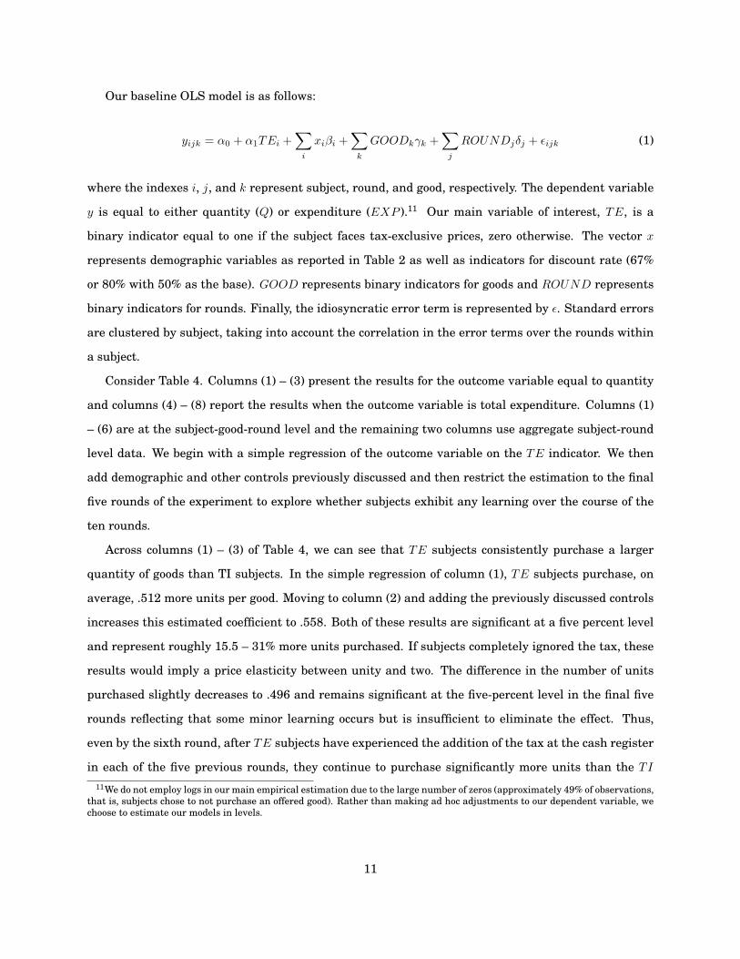
Our baseline OLS model is as follows:

yijk = α0 + α1TEi +�

i

xiβi +�

k

GOODkγk +�

j

ROUNDjδj + �ijk (1)

where the indexes i, j, and k represent subject, round, and good, respectively. The dependent variable

y is equal to either quantity (Q) or expenditure (EXP ).11 Our main variable of interest, TE, is a

binary indicator equal to one if the subject faces tax-exclusive prices, zero otherwise. The vector x

represents demographic variables as reported in Table 2 as well as indicators for discount rate (67%

or 80% with 50% as the base). GOOD represents binary indicators for goods and ROUND represents

binary indicators for rounds. Finally, the idiosyncratic error term is represented by �. Standard errors

are clustered by subject, taking into account the correlation in the error terms over the rounds within

a subject.

Consider Table 4. Columns (1) – (3) present the results for the outcome variable equal to quantity

and columns (4) – (8) report the results when the outcome variable is total expenditure. Columns (1)

– (6) are at the subject-good-round level and the remaining two columns use aggregate subject-round

level data. We begin with a simple regression of the outcome variable on the TE indicator. We then

add demographic and other controls previously discussed and then restrict the estimation to the final

five rounds of the experiment to explore whether subjects exhibit any learning over the course of the

ten rounds.

Across columns (1) – (3) of Table 4, we can see that TE subjects consistently purchase a larger

quantity of goods than TI subjects. In the simple regression of column (1), TE subjects purchase, on

average, .512 more units per good. Moving to column (2) and adding the previously discussed controls

increases this estimated coefficient to .558. Both of these results are significant at a five percent level

and represent roughly 15.5 – 31% more units purchased. If subjects completely ignored the tax, these

results would imply a price elasticity between unity and two. The difference in the number of units

purchased slightly decreases to .496 and remains significant at the five-percent level in the final five

rounds reflecting that some minor learning occurs but is insufficient to eliminate the effect. Thus,

even by the sixth round, after TE subjects have experienced the addition of the tax at the cash register

in each of the five previous rounds, they continue to purchase significantly more units than the TI

11We do not employ logs in our main empirical estimation due to the large number of zeros (approximately 49% of observations,that is, subjects chose to not purchase an offered good). Rather than making ad hoc adjustments to our dependent variable, wechoose to estimate our models in levels.

11

subjects.12 Total expenditures exhibit a similar pattern in columns (4) – (6). The amount spent per

good is 1.03 NIS more for TE subjects, increases to 1.14 NIS once adding the controls and then falls

to .985 in the final five rounds. The first two estimated effects are significant at the five-percent level,

while only the latter estimate is significant at the ten-percent level.

Column (7) of the same table presents the results aggregated over the round. TE subjects spent,

on average, 5.62 more than TI subjects.13 Column (8) presents a slightly different outcome variable.

Recall that subjects always have the option to, and are sometimes forced to, return to their carts. This

could happen for a number of reasons. First, subjects may exceed their budget. This happened ex-

clusively with the TE treatment as subjects may have forgotten, ignored or inaccurately calculated

how much tax would be added to their shopping basket. In such cases, subjects are required to return

to their baskets and remove one or more items in order to remain within their 50-NIS, tax-inclusive

budget constraint. Second, subjects may have second thoughts about a purchase or may simply be

curious to see what happens when they move back and forth between the checkout and the basket.

Nothing in the instructions or in the software prevents subjects from moving back and forth between

the two screens as many times as they choose. Over the 1200 subject-rounds (120 subjects over 10

rounds), 65 distinct subjects in a total of 179 rounds went back to their cart after beginning the check-

out process. Of those 179 revisions, 151 were by TE subjects and 28 by TI subjects. Fifty of these

rounds were imposed due to having exceeded the budget (all of which were TE subjects). Conditional

upon returning to their cart, most subjects returned only once and the maximum number of times that

any one subject went back and forth in a given round was seven. We also collected total round-level

expenditure for these cases of multiple checkouts. This data is useful because, in cases where the

subject was required to return to his basket due to exceeding his budget, the first, non-final checkout

attempt may represent more of an unconstrained demand. We report these results in the final column

of Table 4. The estimated impact of the TE treatment is now larger at 5.96 NIS, suggesting that prior

estimates are somewhat biased down due to the budget constraint forcing some TE subjects to reduce

their expenditures below their desired amounts.

Finally, we reestimated Table 4 where we restricted the sample to those subjects (76% of the total

sample) who, in the post-experiment questionnaire, knew the correct rate of the VAT. The results

(unreported but available upon request) come out even stronger. The point estimates on TE are larger12We will analyze the results by round in depth in Section 7.13As previously mentioned, this result is simply a multiple of the finding in column (3). For this reason and for brevity, we

omit the analogous round-level results for quantity.

12

and significant at the 1% level even in the last 5 rounds. This allows us to eliminate the perfectly

rational explanation that some subjects may fully internalize the tax but at an incorrect lower rate.

4.2 The Treatment Effect by Various Subgroups

We augment our baseline model by interacting the TE indicator with a number of potentially in-

teresting divisions of the data. First, we investigate how the treatment effect varies by the discount

rate, second, by absolute differences in prices between TE and TI, third by category of good (junk food,

school supplies and hygiene), and, finally, by elasticity levels. We describe each in turn. There are two

particular effects of interest here. First, conditional upon being in the TE treatment, does the treat-

ment effect vary along some dimension of interest (e.g., discount rate, elasticity)? This is captured by

the estimated coefficient on the interaction term and can be read directly from Table 5. Second, how do

TE and TI compare along this same dimension of interest? This is captured by the linear combination

of the estimated coefficients on TE and the relevant interaction term. The linear combination of the

estimated coefficients are reported in Table 6.

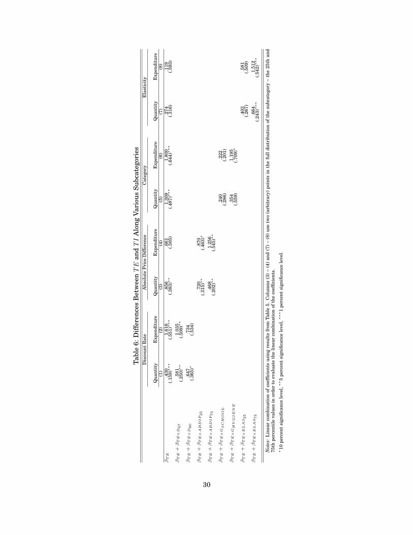
4.2.1 Discount Rates

As previously described, we subjected the prices to three different discount rates – 50%, 67% and

80% – and varied these rates over rounds (but held the discount rate constant within a round). We

interact the TE indicator with indicators for the 67% and 80% discount rates in order to test whether

purchasing behavior differs as price levels change. The quantity and expenditure results are reported

in columns (1) and (2) of Table 5, respectively. As shown by the estimated coefficients on the binary

indicators for the 67% (D67) and 80% (D80) discount rates, subjects overall purchase a larger number

of units and increase their expenditures when discount rates are higher (i.e., when prices are lower).

Moreover, from column (1) we observe that as discount rates increase, the average number of goods

that TE subjects purchase relative to TI subjects increases but this effect is not statistically significant.

Column (2), however, shows an increasing negative effect on expenditures as discount rates increase.14

Moving to Table 6, the estimated coefficients from the first two columns show that for each discount

rate, TE subjects purchase statistically significantly more items and have higher expenditures than TI

subjects with the exception of the of the 80% discount rate where the effect is weaker (and disappears14One way to reconcile this is that TE subjects are purchasing relatively higher quantities of goods but also switching to lower

priced goods so that expenditures are overall decreasing.

13

for expenditures). Thus, when goods are relatively cheap, the effect of tax-exclusive pricing tends to

fade away.

4.2.2 Absolute Price Differences

The differences between the tax inclusive and exclusive prices are always equal to the amount of

the VAT – 16%. However, the absolute difference depends on the price levels that were presented in

Table 1. The absolute differences range from .08 NIS for the energy bar at an 80% discount level to

1.42 NIS for the deodorant at a 50% discount level. If individuals respond to the absolute difference,

then “ignoring” the tax becomes more costly as the price of the good increases. As a result, we should

see a declining TE treatment effect as the absolute price difference increases.

The results are reported in columns (3) and (4) of the same Tables. Overall, there does not appear

to be a clear finding. As absolute price differences increase, so are prices themselves. This means

that subjects purchase a decreasing number of items and we would expect that the quantity difference

between TE and TI would also fall provided that TE subjects are responding on average to a lower

perceived price. Thus, it is not surprising that this is exactly what we see in column (3) of Table 5.

In column (4), both point estimates on TE and the interaction term are insignificant, though keep in

mind that the estimated coefficient on TE has little interpretable value as it reflects the difference

between TE and TI for an absolute price difference of zero (which is clearly out of sample). From this

we can conclude that subjects do not appear to better internalize the tax as prices increase. In fact, the

positive point estimate suggests otherwise, though the lack of any statistical significance supports the

finding that the treatment effect is flat as the absolute price difference increases.

Turning next to column (3) of Table 6. In order to provide some insight as to how the effect varies

as absolute price differences increase, we calculate the linear combination using two points along

the distribution of absolute differences – the 25th and 75th percentiles. The statistically significant

difference between TE and TI holds for these two points for both quantities and expenditures (and

holds for most all of the entire distribution – unreported but available upon request).

4.2.3 Consumption Categories

As discussed, we have ten goods that can be neatly divided into the three categories of junk food,

school supplies and personal hygiene. These goods differ on many dimensions, such as price, price elas-

ticity and frequency of purchase in everyday life. The base category is junk food, SCHOOL represents

14

the school supply category and HY GIENE the personal hygiene category. The results from columns

(5) and (6) of Tables 5 and 6 show that it is the junk food category that is the primary source of our

baseline results. The estimated coefficient on the base category (TE) is positive and significant at the

one-percent level but the interaction terms are negative and significant at nearly the same magnitude

as the base category. When added together, the results show that the treatment effect remains positive

for the school supply and hygiene categories but there is no statistical difference between TE and TI

(with the exception of expenditures on hygiene where TE subjects spend 1.2 NIS more (significant

at the 10% level)). In sum, the estimated coefficients for the junk food category are relatively large

and strongly significant whereas the results for the other categories are much weaker. We conjecture

that junk food items tend to be impulse purchases that provide immediate gratification and also tend

to have higher elasticities, made especially tempting by lower prices. Goods in the school supplies

and hygiene categories are products that are consumed over a longer time horizon, purchased less

frequently in everyday life, and have lower elasticities on average. For these reasons (and certainly

others) purchases are less sensitive to perceived price differences.

4.2.4 Elasticities

Using only the TI subjects, we estimated the point elasticities for each subject under a linear de-

mand curve for each of the goods and then calculated the average elasticity for each good at each

price-quantity bundle. Holding fixed the fraction of the tax that is internalized by the average subject

and assuming the tax is not fully internalized, we would expect a larger difference between TE and

TI the higher is the elasticity (in absolute value). Columns (7) and (8) of the same Tables report the

results. There are a number of interesting results to point out here. First, consider the estimated coef-

ficient on TE. This estimated coefficient represents the estimated difference between TE and TI when

the elasticity is equal to zero (perfectly inelastic) and hence the interaction term is eliminated. In the

case of a perfectly inelastic good, we would expect no difference between TE and TI because demand

is constant regardless of the price (or whatever the price is perceived to be): behavior ought to be the

same for a price p and a price of p(1 + t). The estimated coefficient is indeed small and insignificant

providing nice validation of the internal consistency of the data. The estimated coefficients on the in-

teraction term show that as elasticities increase (in absolute value), the gap between TE and T1 grows

larger, though this finding is only statistically significant for expenditures. Note that salience itself is

difficult to directly test as we rarely know what price individuals perceive as they make their consump-

15

tion choices. We are left to infer this based upon the outcome variable. At very low elasticity levels,

it may well be that subjects do not take into account the tax when making their purchasing decisions

but we would not be able to capture this because subjects are relatively price insensitive. Empirically

speaking, it would be difficult to conclude any statistically significant difference unless demand was

very precisely estimated. As average elasticity levels grow, TE subjects are more responsive, where,

for example, they spend .581 NIS more and purchase .403 units more at the 25th percentile and spend

1.512 NIS and purchase .664 additional units at the 75th percentile. This latter 75th percentile result

is significant at a one-percent level. Thus, provided that TE subjects are at least partially responsive

to a lower perceived price, we find this reaction to manifest itself more in goods where the price elas-

ticity is larger. Finally, we note that it is difficult to separate elasticity from other characteristics of

the good. Higher elasticity goods, in our experiment, tend to be food items that, outside the lab, are

often impulse purchases that provide immediate gratification. Thus, whether this finding is related to

the elasticity or some other feature that is highly correlated with elasticity is difficult to say.

5 Tax Internalization

The results thus far have established that, on average, subjects facing the tax-exclusive price pur-

chase significantly more units than those facing the tax-inclusive price and a similar finding applies

to expenditures. In this section we seek to provide an estimate of how much of the tax is internalized

by those facing the tax-exclusive price. Does the average subject completely ignore the tax or does he

incorporate some fraction of the tax into his final price calculations (perhaps a rough rule of thumb)?

Another way to put it is that some subjects may completely ignore the tax when making their pur-

chasing decisions, while others may fully incorporate the tax such that the average effect is a weighted

average of the two types in the population. We take a straightforward approach where we make use of

the fact that the tax was equal to a fixed percentage throughout the entire experiment. Consider the

following estimable equation:

log pscij = β0 + β1log qij + β2TE +

�

i

xiγi +�

j

ROUNDjδj + �ij (2)

where psc represents the “shopping cart price” that is equal to p(1 + t) for the TI treatment and p for

the TE treatment. In this specification, we consider the price as the endogenous variable. Thus, con-

16

ditional upon the quantity chosen, each subject has a predicted or perceived price.15 For the baseline

TI treatment, there is no uncertainty as to the final price and differences between actual tax-inclusive

prices and predicted prices simply represent measurement error. However, for the TE treatment, we

are left to estimate the perceived price employed to make consumption decisions. Assuming that TI

and TE subjects face identical demand curves for each good, then when the tax is completely ignored

by the TE subjects, the estimated coefficient on the TE indicator should exactly equal the log of (1 + t)

and, in our case, equal log(1.16) = .148.16

We estimate equation (2) separately for each of the goods. The results are reported graphically in

Figure 1. For each good, the black horizontal bar represents the estimated amount internalized and the

vertical boxes represent the 95% confidence intervals. Thus, for the chocolate bar, only 2.3 percentage

points out of the 16 (the amount of the VAT) were internalized, on average. In other words, only a small

fraction of the total tax was taken into account when calculating final prices. Another way to interpret

this result is that 15% of subjects internalized the tax (equal to .023/.16) while the remaining 85%

completely ignored it when making purchasing decisions. Given that zero is included in the confidence

interval, we cannot reject that all subjects completely ignored the tax. As the figure shows, there is

variation over the goods but no particular pattern by category or price level. The level of internalization

ranges from −.001 (completely ignoring the tax) to .138 (near complete internalization).17 We tested for

a correlation between the ranking of the goods’ point estimates of the amount of tax internalized and

the goods’ elasticity, among other variables. Spearman non-parametric rank correlation tests reveal

that none of these correlations are significant at traditional levels.

The average amount internalized over all goods is five percentage points or roughly one-third of the

subjects completely ignore the inclusion of the tax when making their purchasing decisions and the

remaining two-thirds fully internalize the after-tax price.18 However, with only two exceptions (energy

bar and handcream), we cannot reject that the tax was completely ignored in all cases at a five-percent

level of significance. Moreover, this finding is practically unchanged if we consider only the final five

rounds (unreported but available upon request).15Recall that 49% of our quantity observations are zero. Rather than make ad hoc adjustments to this variable and given that

we treat quantity as exogenous in this section, we simply restrict the estimation to positive quantities.16Recall using the properties of log that log p(1 + t) = log p + log (1 + t).17The level of internalization is calculated as follows: 1.16− exp(−βTE ).18It is noteworthy that this result is nearly identical to that reported in Chetty et al. (2009). They find that individuals respond

to a 10% increase in the tax as they would to a 3.5% increase in price.

17

6 Salience vs. Optimism

As discussed in the Introduction, salience refers to the increased visibility of some features of a

good (price in our case) and reduced visibility of other features. To the best of our knowledge, exper-

imental tests of salience have compared tax-exclusive (or shipping-expense-exclusive) prices to those

that include the tax.

One notable feature lacking in empirical studies of salience is the internal mechanism that drives

the results. Do individuals use simple rules of thumb or heuristics to estimate the final all-inclusive

price? In the context of our experiment, perhaps individuals employ a heuristic whereby they round

the VAT to 10% or 20% or, similarly, round a price of 2.23 NIS to 2 NIS or 2.5 NIS. Simple rounding

ought to lead to as many underestimates as overestimates of the final price on average. Thus, it’s not

obvious that a rounding heuristic should provide the overconsumption result that we, and others, have

found.

In order to sharpen the underlying predictions of salience, we introduce an alternative hypothesis

that we refer to as “optimism.” The social psychology literature reports evidence that individuals tend

to be optimistic in a range of settings.19 In the context of our experiment, optimism may be relevant

when the final price is not displayed to subjects and thus there is room to err in its computation.

According to the optimism hypothesis and in contrast to salience, individuals are aware of the existence

of the tax and even the precise tax rate. However, individuals don’t bother to compute 16% of the posted

price and add this amount to determine the final price. Instead, they apply heuristics that simplify

the computation but in their favor. For example, a 16% tax is routinely computed at some simplified

rate less than 16% (e.g. 10%), while a 16% discount is routinely computed at some simplified rate

greater than 16% (e.g. 20%). The TE treatment, like previous papers that considered a less visible tax,

cannot differentiate between salience and optimism. In the case of salience one may inadvertently not

take the tax into account, whereas in the case of optimism it is more of a conscious mental decision to

downplay the magnitude or impact of the tax. Both predict that individuals overpurchase relative to

the tax-inclusive case.

In an attempt to shed light on this issue, we asked TE subjects in a post-questionnaire to describe

their reaction to having the tax added on at the checkout. Their options were (a) “I had forgotten

and it was a surprise” (18/60 subjects); (b) “roughly what I expected” (35/60 subjects); and (c) “exactly19 See Weinstein (1980) for the classic study on optimism. Moore and Healy (2008) cast doubt on the generalizability of

optimism.

18

what I expected” (7/60 subjects). We reestimated our baseline models from Table 4 using only those

subjects who answered (b) or (c) and the results continue to hold at roughly the same point estimates

and significance levels as before (unreported but available upon request). This finding leans towards

the optimism hypothesis as it suggests that inattentiveness to the tax is not a primary driver of our

main findings because even those subjects who were fully aware that the tax would be added on at the

checkout phase overconsumed relative to TI subjects.

In order to better differentiate between the hypotheses, we introduce a third tax-deduction treat-

ment (TD). We take advantage of the fact that an experiment opposite to TE can be readily conducted

in the laboratory, namely, a higher price is posted during the shopping phase and the tax is deducted

from the price at the checkout. In the TD treatment, salience and optimism provide different direc-

tional hypotheses. The salience hypothesis in TD predicts that subjects should purchase too little if

they do not fully internalize the less visible discount offered at the checkout. By contrast, the optimism

hypothesis predicts that subjects in TD will overestimate the actual amount of the tax refund, thereby

leading to a lower perceived price than in TI. The result is that, according to optimism, subjects in TD

are expected to purchase too much.

As in TE, the TD treatment is comprised of a final total price that is broken down into two parts – a

highly visible part and a less visible part (a deduction in the case of TD). For example, consider the tax-

inclusive price of 1 NIS. We first imposed an additional 16% tax for a shopping cart price of 1.16 NIS.

Subjects see this price and are then informed that they will receive a VAT refund upon reaching the

checkout. Thus, the subject observes the 1.16 NIS price and (in theory) computes the VAT deduction,

arriving at a final price of 1 NIS. Thus, while subjects in the TE treatment approach the tax-inclusive

price from below, those in the TD treatment approach the tax-inclusive price from above.

We augment equation (1) with an additional binary indicator, TD, that equals one if the subject

participated in the TD treatment and zero otherwise. Results are reported in Table 7. The baseline

continues to be the TI treatment. We now estimate the effects of the TE and TD treatments in one

equation. The structure of Table 7 is identical to that of Table 4. The effect of the TE treatment is

little changed with the addition of the new treatment (as expected given that these treatments are

independent). Consider next the second row of the Table. Contrary to what the salience and opti-

mism hypotheses would predict, TD subjects show no statistically significant difference in purchasing

decisions from TI subjects. The point estimates are overall much smaller than those in TE, vary be-

tween positive and negative signs and are not significant at any conventional level of significance. We

19

conclude that TD subjects completely internalize the tax discount.

These results pose an interesting question. If we view the issue of salience as “shrouded attributes”,

why does it work in only one direction? Alternatively, if subjects are optimistic, then, again, why only

so when estimating taxes and not discounts? That is, why, on average, do subjects appear not to fully

internalize a tax but yet have little or no difficulty fully internalizing a discount, and, perform the

calculations rather accurately? One potential answer is that with the ubiquity of taxes individuals

have become so accustomed to them that they are an accepted and ignored part of the price. Discounts,

on the other hand, are rarer and thus make more of an impression upon the individual. As a result,

the attentive subject accurately calculates the post-deduction, final price. Although beyond the scope

of this paper, the role of the framing of price components is a fruitful direction for future research.

7 The Treatment Effect by Round

Another feature of our experimental design is that it provides repeated observations of the same

individuals. In fact, our design yields ten separate estimates of our treatment effect, one for each

round. Perhaps higher purchases in TE are driven by initial inattentiveness to the addition of the tax

at the checkout. If so, then ten full repetitions of the experiment and the option to go back and forth

between the checkout and cart in each round as many times as the subject pleases provide subjects

with ample opportunities to correct their initial inattentiveness and to internalize fully the tax. To

illustrate, suppose in round 1 of TE a subject, oblivious to the tax, spends 20 NIS in the first shopping

stage, expecting to pocket 30 NIS. Upon reaching the checkout the subject ought to be surprised to see

that his purchases cost 23.6 NIS, leaving only 26.4 NIS in change. The subject can promptly return to

the shopping stage of round 1 to remove items from his cart. Even if the subject cannot be bothered to

return to the shopping stage, then at least we would expect him to revise downward his purchases in

round 2. To our knowledge, the current literature is agnostic about the effect of salience in a dynamic

environment that provides opportunities for learning. The results are presented in Figure 2 where we

run the full models from columns (2) and (5) of Table 7.

Panel (a) presents the results for TE and TD for the dependent variable of quantity per good

relative to TI and Panel (b) presents the analogous graph for the dependent variable of expenditure

per good relative to TI. The black horizontal bars represent the point estimates and the vertical bars

20

the 90% confidence intervals.20 Consider first Panel (a). The estimated coefficient on TE does not show

any clear downward trend over the ten rounds but there are four rounds, concentrated in the latter

half of the experiment, that are not significant at even the 10% level – rounds 5, 7, 8, and 10.21 Three

of these rounds (5, 7 and 10) also have much smaller point estimates (in the range .21 – .26) than other

rounds. Thus, it appears that some subjects began to internalize the tax as they gained experience in

the experiment. Still, the figure does not conclusively show that learning was particularly strong.

TD, on the other hand, presents a consistent picture across rounds. The point estimates are rela-

tively small, cycle between positive and negative and, from the outset, are never significantly different

from zero at even the 10% level.

Turning to Panel (b), expenditures paint a similar picture for TE but round 8 is now significant at

the 10% level; rounds 5, 7 and 10 continue not to be. TD round-level results show a lack of significance

across the board, as with quantity. In sum, for TE subjects the treatment effect shows some signs of

weakening in later rounds but does not disappear altogether. TD subjects consistently internalize the

VAT discount.

8 Conclusions

In the broadest sense, our experiment tests for a tax-framing effect on consumer demand: three

identical scenarios differ merely in the way the price is presented to subjects. The tax frame ought

not to matter since the products’ final prices are identical across treatments. And yet consistent with

recent literature showing that not all price components are treated equally, we too find differences in

consumer demand across tax treatments. Most importantly, and confirming the results of Chetty et

al., subjects buy more under a tax-exclusive regime than under an equivalent tax-inclusive regime.

The salience of the tax is one explanation for this result and is also consistent with theories (or rules

of thumb) other than salience. Optimism is an alternative hypothesis according to which individuals

underestimate taxes and overestimate discounts. Both salience and optimism predict that individuals

should overconsume when facing tax-exclusive pricing relative to tax-inclusive pricing. To differenti-

ate between the hypotheses, we introduce a third tax-deduction treatment in which a price component20We use the more liberal 10% level of significance here for two reasons: (1) Tables 4 and 7 already have shown that the TE

effect is slightly weaker in the second half of the rounds. Thus, we anticipate there are rounds that are significant only at a 10%level and we wanted to capture this fact; (2) we also saw in Table 7 that TD was not statistically significant. Thus, a 10% levelmay allow us to capture individual rounds that may be marginally significant.

21Recall that the goods offered were completely balanced across rounds so differences cannot be due to differences in thecomposition of goods by round across treatments.

21

(the tax) is subtracted from the final price. The results from this treatment reveal that salience may

not be the key explanation for the hereto observed finding that price partitioning leads to higher de-

mand as we cannot reject that subjects who face tax-deduction prices consume the same as those who

face tax-inclusive prices. Moreover, consumer optimism also does not account for our findings. We

are therefore left with a open question as to why individuals appear not to internalize fully tax pay-

ments but do internalize tax refunds. One plausible answer consistent with our findings as well as

those of Hossain and Morgan (2006) and Brown, Hossain and Morgan (2010) is that some price compo-

nents such as shipping-and-handling charges and taxes are taken for granted and seen as unavoidable.

Thus, individuals tend not to heed and even ignore these commonplace, inescapable price components.

Because tax discounts are far less ubiquitous, they elicit the attention of the individual and induce

him to give some thought to the final price. Finally, over the ten-round time frame of our experiment,

the treatment effect shows some signs of weakening, although does not completely disappear, whereas

subjects appear to internalize the tax deduction from the outset and through the entire duration of the

experiment.

The short-run policy implications are numerous. First, the necessary tax rate that raises a given

amount of tax revenue is lower in the case of tax-exclusive pricing as compared to tax-inclusive pricing

as consumers adjust their behavior less in the latter case, thus resulting in a more efficient second-

best outcome.22 Second, given that a tax is not fully internalized, the government can choose between

a VAT or sales-tax style tax based upon whether it aims to discourage a taxed activity. For example,

sin taxes or taxes on goods that impose a negative externality are best implemented in the VAT form

whereas taxes on goods that are complementary with labor are best implemented with a sales tax.

Third, switching from a VAT to a sales-tax regime during an economic downturn may provide short-

term stimulus to the economy, that is, increase consumption and government revenues while leaving

producers no worse off provided increased government revenues are partially used for compensation.

The long run is less clear. On one hand, the lack of internalization allows a greater proportion of the

tax to be shifted onto the consumer. Producers benefit as the after-tax price they receive is higher, as

is demand. On the other hand, our experiment suggests that, over time, the impact of any government

manipulation of how the tax is imposed may become less effective, though not disappear entirely.22We assume here standard upward sloping supply and downward sloping demand curves.

22

References

Anderson, Eric T. and Duncan I. Simester (2003) “Effects of $9 Price Endings on Retail Sales: Evi-

dence from Field Experiments,” Quantitative Marketing and Economics, 1, 93-110.

Barber, Brad, Terrance Odean and Lu Zheng (2005) “Out of Sight, Out of Mind: The Effects of Ex-

penses on Mutual Fund Flows,” Journal of Business, 78, 2095-2119.

Blumkin, Tomer, Bradley J. Ruffle and Yosef Ganun (2011) “Are Income and Consumption Taxes

Ever Really Equivalent? Evidence from a Real-Effort Experiment with Real Goods,” unpublished

manuscript.

Brown, Jennifer, Tanjim Hossain and John Morgan (2010) “Shrouded Attributes and Information

Suppression,” Quarterly Journal of Economics, 125:2, 859-876.

Carlin, Bruce I. (2009) “Strategic price complexity in retail financial markets,” Journal of Financial

Economics, 91, 278-287.

Chetty, Raj, Adam Looney and Kory Kroft (2009) “Salience and Taxation: Theory and Evidence,”

American Economic Review, 99:4, 1145-1177.

Feldman, Naomi and Peter Katuscak (2009) “Effects of Predictable Tax Liability Variation on House-

hold Labor Income,” unpublished manuscript.

Finkelstein, Amy (2009) “EZ-Tax: Tax Salience and Tax Rates,” Quarterly Journal of Economics,

124:3, 969-1010.

Gabaix, Xavier and David Laibson (2006) “Shrouded Attributes, Consumer Myopia, and Information

Suppression in Competitive Markets,” Quarterly Journal of Economics, 121:2, 505-540.

Hossain, Tanjim and John Morgan (2006) “...Plus Shipping and Handling: Revenue (Non) Equiva-

lence in Field Experiments on eBay,” B.E. Press Advances in Economic Analysis & Policy, 6:2,

Article 3.

Kalayci, Kenan and Jan Potters (2011) “Buyer confusion and market prices,” International Journal of

Industrial Organization, 29:1, 14-22.

Kalayci, Kenan (2011) “Price complexity and buyer confusion in markets,” unpublished manuscript.

23

Moore, Don A. and Paul J. Healy (2008) “The Trouble with Overconfidence,” Psychological Review,

115:2, 502-517.

Morwitz, Vicki G., Eric A. Greenleaf and Eric J. Johnson (1998) “Divide and Prosper: Consumers’

Reactions to Partitioned Prices,” Journal of Marketing Research, 35:4, 453-463.

Weinstein, Neal D. (1980) “Unrealistic optimism about future life events,” Journal of Personality and

Social Psychology, 39:5, 806-820.

24

Table 1: Pre-sales-tax and Pre-discount Prices of Goods in the ExperimentJunk Food

Energy Bar 2.65Chocolate Bar 5.54Pack of Gum 3.70

School SuppliesHighlighter 2.86Pen 6.80Pad of Paper 5.97

HygieneHandcream 12.56Deodorant 17.73Toothbrush 5.03Toothpaste 13.36

Notes: Retail prices (not including the sales tax) in New Israeli Shekels (1 USD = 3.6 NIS) for each of the ten goods used inthe experiment.

25

Table 2: Socio-Demographic Summary Statistics

Treatment TE TI TD Kruskal-Wallis test

VariableMean Mean Mean χ2(2)

(Std. Dev.) (Std. Dev.) (Std. Dev.) p-valueMale .500 .450 .550 0.90

(.500) (.498) (.498) .64Age 25.32 24.93 25.03 1.35

(1.68) (1.75) (3.33) .51Undergrad .900 .967 .983 0.70

(.302) (.181) (.128) .71Economics Major .150 .183 .233 0.63

(.357) (.387) (.423) .73Engineering Major .617 .517 .417 3.58

(.486) (.500) (.493) .17Other Major .233 .300 .350 1.23

(.423) (.458) (.477) .54Obs. (Subjects) 60 60 60

Notes: The last column reports the results of a non-parametric, rank-sum Kruskal-Wallis tests comparing the three treat-ments for each of the variables.

26

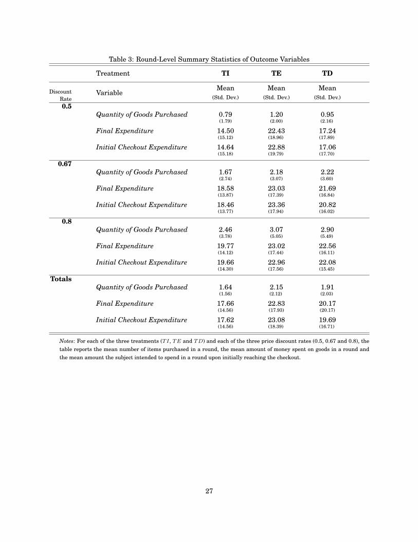
Table 3: Round-Level Summary Statistics of Outcome Variables

Treatment TI TE TD

Discount VariableMean Mean Mean

Rate (Std. Dev.) (Std. Dev.) (Std. Dev.)

0.5

Quantity of Goods Purchased 0.79 1.20 0.95(1.79) (2.00) (2.16)

Final Expenditure 14.50 22.43 17.24(15.12) (18.96) (17.89)

Initial Checkout Expenditure 14.64 22.88 17.06(15.18) (19.79) (17.70)

0.67




0.8




Totals




Notes: For each of the three treatments (TI, TE and TD) and each of the three price discount rates (0.5, 0.67 and 0.8), thetable reports the mean number of items purchased in a round, the mean amount of money spent on goods in a round andthe mean amount the subject intended to spend in a round upon initially reaching the checkout.

27

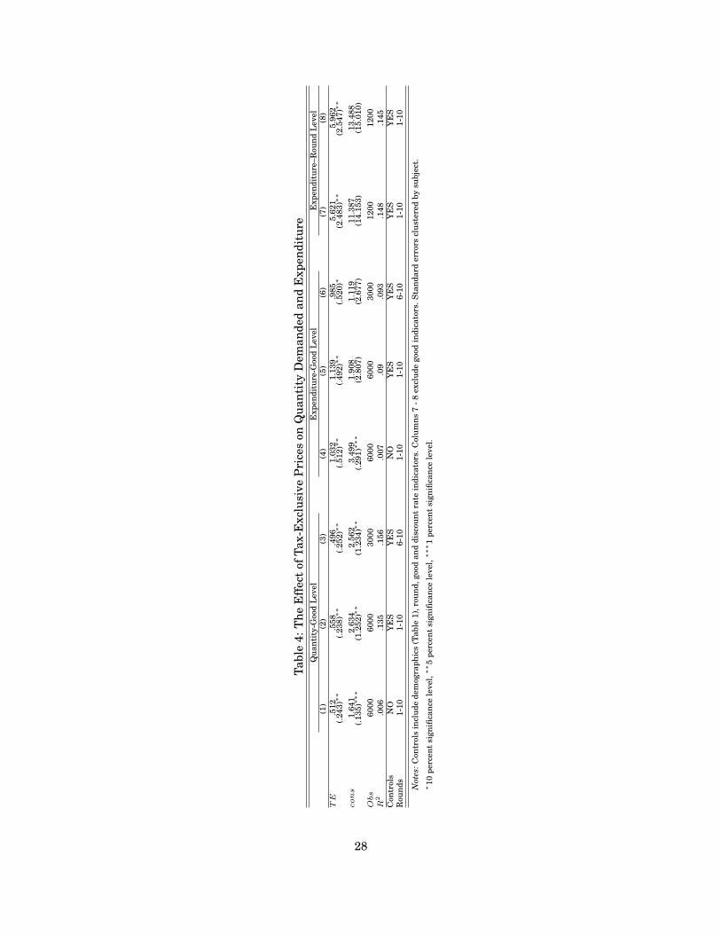
Tabl

e4:

The

Effe

ctof

Tax-

Exc

lusi

vePr

ices

onQ

uant

ity

Dem

ande

dan

dE

xpen

ditu

reQ

uant

ity-

Goo

dLe

vel

Exp

endi

ture

-Goo

dLe

vel

Exp

endi

ture

–Rou

ndLe

vel

(1)

(2)

(3)

(4)

(5)

(6)

(7)

(8)

TE

.512

.558

.496

1.03

21.

139

.985

5.62

15.

962

(.243

)∗∗

(.238

)∗∗

(.252

)∗∗

(.512

)∗∗

(.492

)∗∗

(.520

)∗(2

.483

)∗∗

(2.5

47)∗∗

con

s1.

641

2.63

42.

562

3.49

91.

908

1.11

911

.387

13.4

88(.1

35)∗∗∗

(1.2

52)∗∗

(1.2

34)∗∗

(.291

)∗∗∗

(2.8

07)

(2.6

77)

(14.

153)

(15.

010)

Obs

6000

6000

3000

6000

6000

3000

1200

1200

R2

.006

.135

.156

.007

.09

.093

.148

.145

Con

trol

sN

OY

ES

YE

SN

OY

ES

YE

SY

ES

YE

SR

ound

s1-

101-

106-

101-

101-

106-

101-

101-

10

Not

es:C

ontr

ols

incl

ude

dem

ogra

phic

s(T

able

1),r

ound

,goo

dan

ddi

scou

ntra

tein

dica

tors

.Col

umns

7-8

excl

ude

good

indi

cato

rs.S

tand

ard

erro

rscl

uste

red

bysu

bjec

t.∗

10pe

rcen

tsig

nific

ance

leve

l,∗∗

5pe

rcen

tsig

nific

ance

leve

l,∗∗∗

1pe

rcen

tsig

nific

ance

leve

l.

28

Tabl

e5:

The

Effe

ctof

Tax-

Exc

lusi

vePr

ices

onQ

uant

ity

Dem

ande

dan

dE

xpen

ditu

re(b

ySu

bcat

egor

y)D

isco

untR

ate

Abs

olut

ePr

ice

Diff

eren

ceC

ateg

ory

Ela

stic

ity

(Abs

olut

eVa

lue)

Qua

ntit

yE

xpen

ditu

reQ

uant

ity

Exp

endi

ture

Qua

ntit

yE

xpen

ditu

reQ

uant

ity

Exp

endi

ture

(1)

(2)

(3)

(4)

(5)

(6)

(7)

(8)

TE

.430

1.61

6.8

56.6

611.

309

1.80

0.2

74.1

19(.1

59)∗∗∗

(.551

)∗∗∗

(.383

)∗∗

(.505

)(.4

87)∗∗∗

(.644

)∗∗∗

(.316

)(.5

93)

D67

.855

.838

(.105

)∗∗∗

(.227

)∗∗∗

D80

1.66

21.

073

(.150

)∗∗∗

(.310

)∗∗∗

TE×

D67

.151

-.581

(.156

)(.3

34)∗

TE×

D80

.216

-.882

(.278

)(.3

89)∗∗

AB

DIF

-1.2

862.

591

(.242

)∗∗∗

(.748

)∗∗∗

TE×

AB

DIF

-.712

1.09

1(.3

87)∗

(.907

)S

CH

OO

L-.8

26-.1

41(.3

03)∗∗∗

(.485

)H

YG

IE

NE

-1.1

651.

047

(.225

)∗∗∗

(.447

)∗∗

TE×

SC

HO

OL

-1.0

69-1

.446

(.489

)∗∗

(.721

)∗∗

TE×

HY

GIE

NE

-1.0

87-.6

04(.4

31)∗∗

(.681

)E

LA

S1.

878

1.84

7(.5

93)∗∗∗

(1.3

31)

TE×

EL

AS

1.16

74.

174

(.788

)(1

.717

)∗∗

con

s1.

170

2.26

81.

879

2.04

51.

985

.770

.498

1.79

6(1

.199

)(2

.746

)(1

.228

)(2

.742

)(1

.227

)(2

.747

)(1

.235

)(2

.810

)O

bs60

0060

0060

0060

0060

0060

0060

0060

00R

2.0

77.0

41.1

3.0

53.0

97.0

6.0

87.0

49

Not

es:

Bas

eca

tego

ries

:D

isco

unt

rate

(50%

),ca

tego

ry(ju

nkfo

od).

Stan

dard

erro

rscl

uste

red

bysu

bjec

t.∗

10pe

rcen

tsi

gnifi

canc

ele

vel,∗∗

5pe

rcen

tsi

gnifi

canc

ele

vel,∗∗∗

1pe

rcen

t

sign

ifica

nce

leve

l.

29

Tabl

e6:

Diff

eren

ces

Bet

wee

nT

Ean

dT

IA

long

Vari

ous

Subc

ateg

orie

sD

isco

untR

ate

Abs

olut

ePr

ice

Diff

eren

ceC

ateg

ory

Ela

stic

ity

Qua

ntit

yE

xpen

ditu

reQ

uant

ity

Exp

endi

ture

Qua

ntit

yE

xpen

ditu

reQ

uant

ity

Exp

endi

ture

(1)

(2)

(3)

(4)

(5)

(6)

(7)

(8)

βT

E.4

301.

616

.856

.661

1.30

91.

800

.274

.119

(.159

)∗∗∗

(.551

)∗∗∗

(.383

)∗∗

(.505

)(.4

87)∗∗∗

(.644

)∗∗∗

(.316

)(.5

93)

βT

E+

βT

E×

D67

.581

1.03

5(.2

50)∗∗

(.509

)∗∗

βT

E+

βT

E×

D80

.647

.734

(.365

)∗(.5

34)

βT

E+

βT

E×

AB

DI

F25

.720

.870

(.315

)∗∗

(.463

)∗

βT

E+

βT

E×

AB

DI

F75

.468

1.25

6(.2

02)∗∗

(.545

)∗∗

βT

E+

βT

E×

GS

CH

OO

L.2

40.2

22(.2

86)

(.201

)β

TE

+β

TE×

GH

YG

IE

NE

.354

1.19

5(.5

59)

(.709

)∗

βT

E+

βT

E×

EL

AS25

.403

.581

(.267

)(.5

09)

βT

E+

βT

E×

EL

AS75

.664

1.51

2(.2

43)∗∗∗

(.542

)∗∗∗

Not

es:

Line

arco

mbi

nati

onof

coef

ficie

nts

usin

gre

sult

sfr

omTa

ble

5.C

olum

ns(3

)–(4

)and

(7)–

(8)u

setw

o(a

rbit

rary

)poi

nts

inth

efu

lldi

stri

buti

onof

the

subc

ateg

ory

–th

e25

than

d75

thpe

rcen

tile

valu

esin

orde

rto

eval

uate

the

linea

rco

mbi

nati

onof

the

coef

ficie

nts.

∗10

perc

ents

igni

fican

cele

vel,∗∗

5pe

rcen

tsig

nific

ance

leve

l,∗∗∗

1pe

rcen

tsig

nific

ance

leve

l.

30

Tabl

e7:

The

Effe

ctof

Tax-

Exc

lusi

vean

dTa

x-D

educ

tion

Pric

eson

Qua

ntit

yD

eman

ded

and

Exp

endi

ture

sQ

uant

ity-

Goo

dLe

vel

Exp

endi

ture

-Goo

dLe

vel

Exp

endi

ture

–Rou

ndLe

vel

(1)

(2)

(3)

(4)

(5)

(6)

(7)

(8)

TE

.512

.553

.488

1.03

21.

140

.986

5.65

95.

997

(.242

)∗∗

(.236

)∗∗

(.250

)∗(.5

11)∗∗

(.490

)∗∗

(.519

)∗(2

.467

)∗∗

(2.5

25)∗∗

TD

.102

.045

-.011

.063

-.083

-.154

-.483

-.755

(.214

)(.2

16)

(.228

)(.4

42)

(.446

)(.4

72)

(2.2

29)

(2.2

08)

con

s1.

641

3.91

23.

673

3.49

93.

793

2.71

318

.812

21.1

98(.1

35)∗∗∗

(1.0

68)∗∗∗

(.993

)∗∗∗

(.290

)∗∗∗

(2.2

07)∗

(2.0

04)

(10.

860)∗

(11.

366)∗

Obs

9000

9000

4500

9000

9000

4500

1800

1800

R2

.004

.12

.135

.006

.077

.08

.091

.095

Con

trol

sN

OY

ES

YE

SN

OY

ES

YE

SY

ES

YE

SR

ound

s1-

101-

106-

101-

101-

106-

101-

101-

10

Con

trol

s:D

emog

raph

ics

(Tab

le1)

.C

olum

ns2

–6

incl

ude

roun

din

dica

tors

,goo

din

dica

tors

,goo

dta

ble

indi

cato

rs.

Col

umns

7–

8in

clud

ero

und

indi

cato

rs.

Col

umns

2–

3in

clud

epr

ice

(wit

hVA

T)an

dco

lum

ns5

–8

incl

ude

disc

ount

rate

indi

cato

rs.S

tand

ard

erro

rscl

uste

red

bysu

bjec

t.∗

10pe

rcen

tsig

nific

ance

leve

l,∗∗

5pe

rcen

tsig

nific

ance

leve

l,∗∗∗

1pe

rcen

tsig

nific

ance

leve

l.

31

Figure 1: The Amount of Internalized Tax (0 - 16%)

-0.1

-0.05

0

0.05

0.1

0.15

0.2

0.25

-0.1

-0.05

0

0.05

0.1

0.15

0.2

0.25

Notes: The figure displays the amount (in percentage points) of the VAT that is internalized, on average, for each good. Zeroreflects that the tax is completely ignored, whereas .16 represents all of the tax being internalized. The black horizontal bardisplays the mean mean amount internalized, with the vertical bars indicating 95% confidence intervals.

32

Figure 2: Treatment Effect by Round (1-10)

(a) Quantity Purchased per good relative to TI

(b) Quantity Purchased per good relative to TI

Notes: Horizontal lines represent point estimates and vertical bars represent 90% confidence intervals. Light colored barsrepresent TE and darker colored bars represent TD.

33

Appendix

Figure 3: Tax-Inclusive Pricing

(a) Cart

(b) Check out

Notes: Cart and checkout screen shots for the tax-inclusive treatment for a randomly chosen bundle of goods.

34

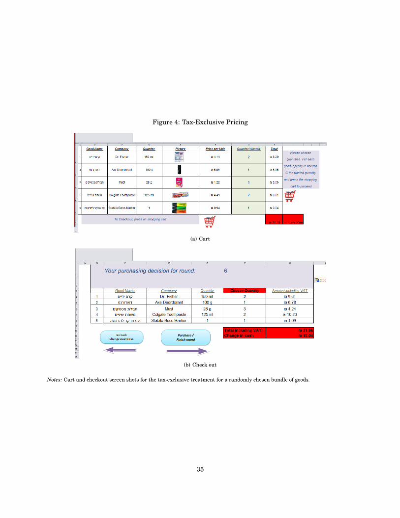
Figure 4: Tax-Exclusive Pricing

(a) Cart

(b) Check out

Notes: Cart and checkout screen shots for the tax-exclusive treatment for a randomly chosen bundle of goods.

35

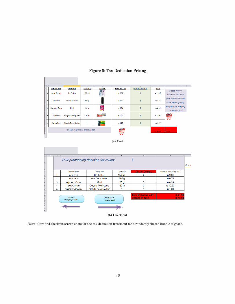
Figure 5: Tax-Deduction Pricing

(a) Cart

(b) Check out

Notes: Cart and checkout screen shots for the tax-deduction treatment for a randomly chosen bundle of goods.

36

* Notes to reader: (1) the instructions are identical for all three treatments except where noted. Text

within parentheses differentiates between the [TI], (TE) and TD treatments. (2) the bolded text also

appears bolded in the Hebrew instructions given to subjects.

Participant Instructions

This is an experiment in individual decision-making. There are no correct or incorrect decisions in this

experiment. Your decisions are a matter of your personal tastes. We are interested to learn your tastes

and how you make purchasing decisions. Your decisions determine the payment that you will receive

at the end of the experiment. We ask that you make all decisions on your own without consulting or

discussing the experiment with anyone else.

This experiment consists of ten rounds. In each round, you will be given 50 NIS. You will be shown a

number of goods, each at a discounted price. [The prices all include VAT and are the final prices.]

(The prices do not include VAT. When you proceed to the checkout, the VAT will be added

to these prices to determine the final prices.) The prices include VAT. When you proceed to

the checkout, the VAT will be deducted from these prices to determine the final prices.

In each round, you will be asked to allocate your 50 NIS as you like between the goods that are

displayed. You are free to purchase as many or as few units of each good as you choose. But you may

not exceed your 50 NIS budget [after the addition of the VAT] after the deduction of the VAT. You will

receive at the end of the experiment all of the goods that you purchased, each according to the quantity

that you chose. You may spend all, some or none of your 50 NIS on these goods. Whatever money you

don’t spend is yours to keep.

The decision how to allocate your initial 50 NIS endowment will be repeated over ten rounds. The

only difference between the ten rounds is the composition of the goods available for purchase in each

round and the prices of the goods. At the end of the experiment, one of the ten rounds will be randomly

selected and you will be paid according to the choices you made in that round. You will receive the

quantities of all of the goods that you chose to purchase that round and any money from the initial

50 NIS that you didn’t spend from that round. We have discounted the goods such that you can earn

anywhere between 50 NIS in cash and 250 NIS worth of goods.

In each round, after you have decided how you wish to allocate your 50 NIS, please press on the

shopping cart icon to continue to the checkout stage where you may confirm or adjust your choices

before continuing to the next round.

37

The Impact of Tax Exclusive and Inclusive Prices on...

Documents

Transcript of The Impact of Tax Exclusive and Inclusive Prices on...