The Impact of Selection on the Genome

D. M. Howard

Introduction

• Historically pedigree used to manage genetic diversity

Assumes selection-free, neutral loci

• Loci close to QTL will have higher loss of diversity

Roughsedge et al. (2008) Genetics Research, 90:199-208

Sonesson et al. (2012) Genetics Selection Evolution, 44:27

Rationale

• With high density data we can:

1. Identify regional variations in selection

2. Examine level of conformity with pedigree model

Aims

Materials & Methods

• Line A

Reproductive traits & growth rate

1,551 genotyped individuals over 6 generations

39,377 SNPs

• Line B

Reproductive traits

4,889 genotyped individuals over 6 generations

40,396 SNPs

• Illumina PorcineSNP60 Beadchip

Data

• Fit a regression for each SNP :

ln(Hij) = ±j + ² j ln(1-Fi) + µij

Model

Model

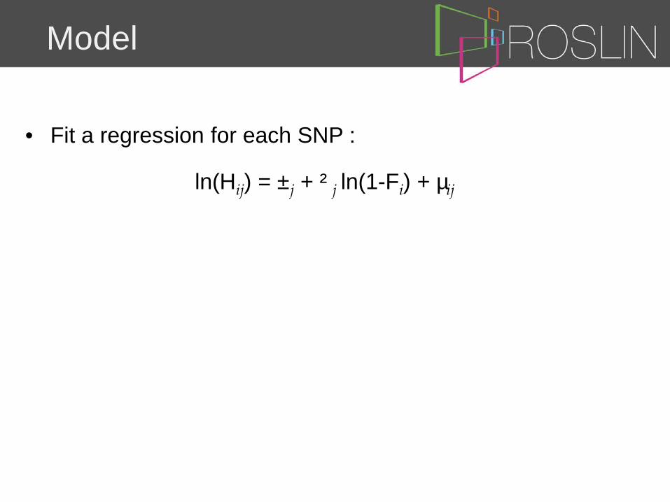
• Fit a regression for each SNP :

ln(Hij) = ±j + ² j ln(1-Fi) + µij

Where,

H = Observed heterozygosity

1-F = Expected heterozygosity

± = Intercept

µ = Error term

² = Slope of the regression

Model

• Fit a regression for each SNP :

ln(Hij) = ±j + ² j ln(1-Fi) + µij

Where,

H = Observed heterozygosity

1-F = Expected heterozygosity

± = Intercept

µ = Error term

² = Slope of the regression

Model

Where,

H = Observed heterozygosity

1-F = Expected heterozygosity

± = Intercept

µ = Error term

² = Slope of the regression

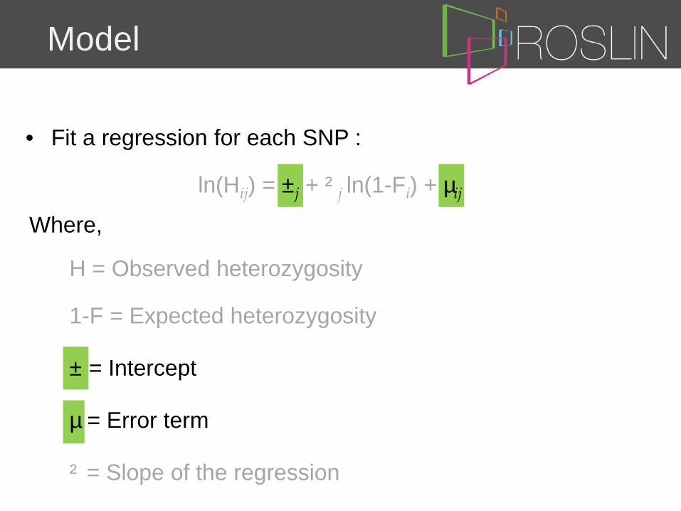
• Fit a regression for each SNP :

ln(Hij) = ±j + ² j ln(1-Fi) + µij

² j = 1, Loss of heterozygosity equals expectation

² j > 1, Loss is greater than expected

² j < 1, Loss is less than expected

Regression slope, ²

• Fit a regression for each SNP :

ln(Hij) = ±j + ² j ln(1-Fi) + µij

Line A, Genome Wide

1 2 3 4 5 6 7 8 9 10 11 12 13 14 15 16 17 18

² j = 1

² j

Chromosome

Line A, Genome Wide

1 2 3 4 5 6 7 8 9 10 11 12 13 14 15 16 17 18

² j

Chromosome

² j = 1

Line A, SSC07

Position, Mb

² j

² j = 1

Confidence Intervals

• Bootstrap using gene-dropping for every SNP

• Use distribution of iterations to form confidence intervals

² j

MAF = 0.23

95% (-0.8, 4.2)

MAF = 0.08

95% (-3.1, 19.0)

² j

Results

Line A, SSC07

Position, Mb

² j

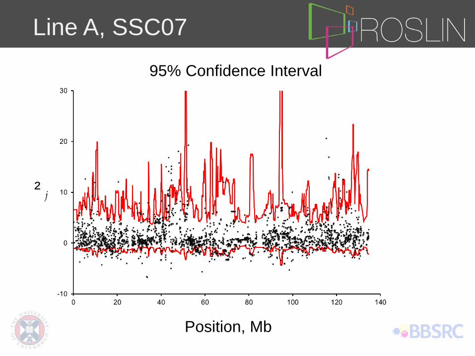
Line A, SSC07

95% Confidence Interval

² j

Position, Mb

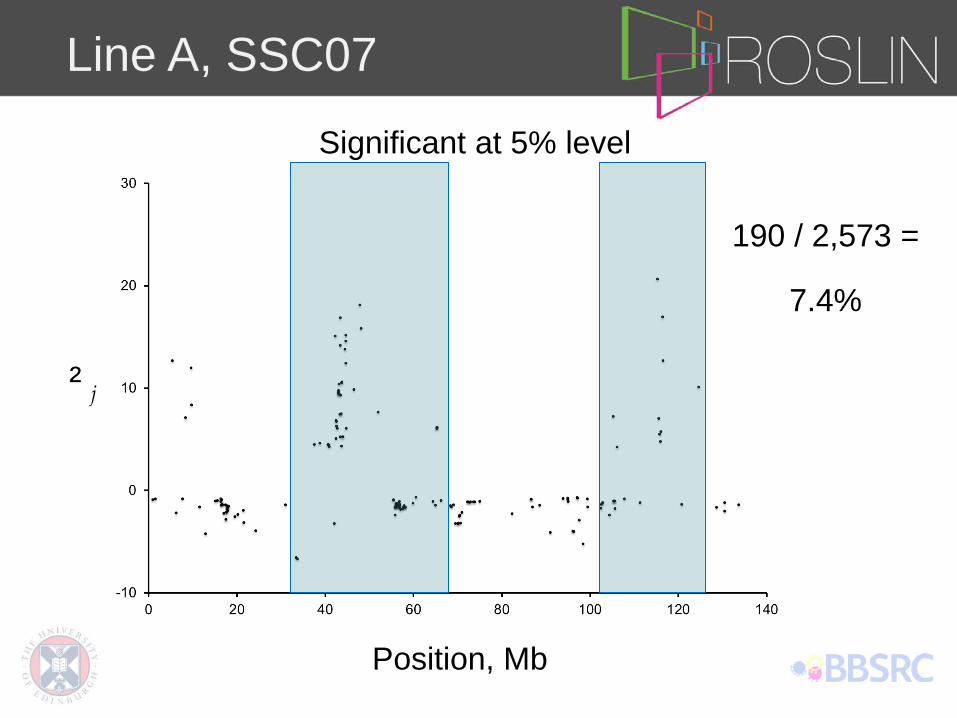
Line A, SSC07

Significant at 5% level

190 / 2,573 =

7.4%

Position, Mb

² j

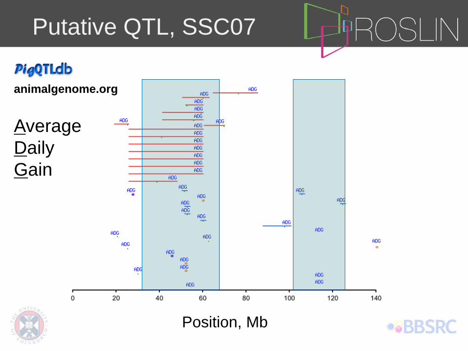
Putative QTL, SSC07

animalgenome.org

Average Daily Gain

Position, Mb

Line Comparison, SSC06

Line A Line B

² j

Position, Mb

Significant at 5% level

² j

Line A Line B

Position, Mb

Changes in Heterozygosity Line A Line B

Confidence Intervals 1% 5% Upper

0.5% Upper 2.5%

Lower 0.5%

Lower 2.5%

Whole Genome 0.86% 4.05% 0.33% 1.59% 0.53% 2.46%

SSC01

SSC02

SSC03

SSC04

SSC05

SSC06

SSC07 7.4% SSC08

SSC09

SSC10

SSC11

SSC12

SSC13

SSC14

SSC15

SSC16

SSC17

SSC18

Confidence Intervals 1% 5% Upper

0.5% Upper 2.5%

Lower 0.5%

Lower 2.5%

Whole Genome 1.70% 6.14% 0.65% 2.66% 1.05% 3.48%

SSC01

SSC02

SSC03

SSC04

SSC05

SSC06

SSC07

SSC08

SSC09

SSC10

SSC11

SSC12

SSC13

SSC14

SSC15

SSC16

SSC17

SSC18

= Evidence for excessive change in heterozygosity

Summation

• With high density data we can:

1. Identify regional variations in selection

2. Examine level of conformity with pedigree model

Aims

Conclusions

• Evidence of diversity loss at specific regions

Putative QTL identification (Line A, SSC07)

• Varying impact between lines (SSC06)

Trait Architecture

Power

Future - Haplotyping

• With high density data we can:

1. Identify regional variations in selection

2. Examine level of conformity with pedigree model

Aims

Implications

• Evidence for inadequacy of pedigree model (Line B)

• Genomic Optimal Contributions

• Precision inbreeding at SNP level

• ‘ ‘ Regional loss of diversity, provided maintained elsewhere

Acknowledgements

John Woolliams Ricardo Pong-Wong

Pieter Knap Valentin Kremer Dave McLaren Olwen Southwood Nan Yu