The Impact of Microfinance on its Beneficiaries:Impact Assessment on Bancamia in Armenia, Colombia

A Thesis

submitted to Aalborg Univeristy

in partial fulfillment of the requirements for the

degree of

Master on Development and International Relations

By

Jesús Olano Espinosa

Aalborg, Denmark

31st of May 2012

Table of Contents

List of Tables ......................................................................................................................4

List of Acronyms .................................................................................................................5

1 INTRODUCTION.........................................................................................................6

1.1 A NOTE ABOUT COLOMBIA..................................................................................6

1.1.1 Geographical Context.................................................................................................6

1.1.2 Social and Economic Context.....................................................................................7

1.2 HISTORICAL ANTECEDENTS OF MICROCREDIT............................................8

1.2.1 Historical Antecedents of Microcredit in Developing Countries..................................9

1.2.2 Historical Antecedents of Microcredit in Europe.......................................................10

1.2.3 The Emergence of Modern Microfinance..................................................................12

1.2.4 Microfinance in Colombia........................................................................................13

2 THEORETICAL FRAMEWORK................................................................................15

2.1 WHY MICROFINANCE?.........................................................................................16

2.1.1 Definition of Microcredit..........................................................................................16

2.1.2 Formal vs. Informal Sector........................................................................................16

2.1.3 The Imperfect Information Paradigm........................................................................18

2.1.3.1 The Imperfect Information Paradigm: Joint Liability vs. Individual Liability...........20

2.2 CONCEPTUAL FRAMEWORK..............................................................................21

2.2.1 The Impact Chain.....................................................................................................21

2.2.2 Units of Assessment...................................................................................................23

2.2.3 Types of Impact........................................................................................................25

2.3 APPLICATION OF THE CONCEPTUAL FRAMEWORK...................................26

2.3.1 The Intermediary School...........................................................................................26

2.3.2 The Intended Beneficiary School..............................................................................27

2.4 MODEL OF THE IMPACT ANALYSIS...................................................................28

2.4.1 Definition of Household...........................................................................................29

2.4.2 Household Level Analysis..........................................................................................30

2.4.3 Intrahousehold Level Analysis....................................................................................33

2.4.3.1 Intrahousehold Level Analysis: Pooled Models.......................................................33

2.4.4 Risk and Coping Response Models...........................................................................34

2.4.4.1 Risk and Coping Response Models: Models of risk................................................35

2.4.4.2 Risk and Coping Response Models: Models of Coping Strategies..........................35

2.4.5.1 The Household Economic Portfolio Model: The Portfolio System.........................37

2.4.5.3 The Household Economic Portfolio Model: Proposed Hypothesis.........................39

2.5 STUDY DESIGN........................................................................................................40

2.5.1 Study Design Theories..............................................................................................41

2.5.1.1 Study Design Theories: The Scientific Method......................................................42

2.5.1.2 Study Design Theories: The Humanities Paradigm.................................................43

2.6 POTENTIAL BIASES.................................................................................................44

2.6.1. Fungibility and Endogeneity.....................................................................................44

2.6.2 Biases Associated with Sample Design.......................................................................46

2.6.3 Biases Associated with Cross-Sectional Analysis.........................................................47

3 METHODOLOGICAL CONSIDERATIONS.............................................................49

3.1 IMPACT ANALYSIS DESIGN..................................................................................49

3.1.1 Units of Assessment...................................................................................................49

3.1.2 Study Hypotheses......................................................................................................50

3.1.3 Types of Impact........................................................................................................51

3.1.3.1 Types of Impact: Domains of Change.....................................................................51

3.1.3.2 Types of Impact: Markers of Change......................................................................51

3.2 IMPLEMENTATION OF THE STUDY DESIGN...................................................52

3.2.1 Considerations about the Implementation.................................................................53

3.2.2 Considerations about Potential Biases........................................................................54

3.3 STATISTICAL METHODOLOGY...........................................................................55

4 ANALYTICAL PART...................................................................................................57

4. 1 Design Implementation...............................................................................................59

4. 2 Ex-ante Analysis..........................................................................................................61

4. 3 Ex-post Analysis..........................................................................................................68

4. 4 Contrast of the Study Hypotheses...............................................................................73

5 CONCLUSSIONS.........................................................................................................76

6 BIBLIOGRAPHY..........................................................................................................78

Internet Resources.............................................................................................................84

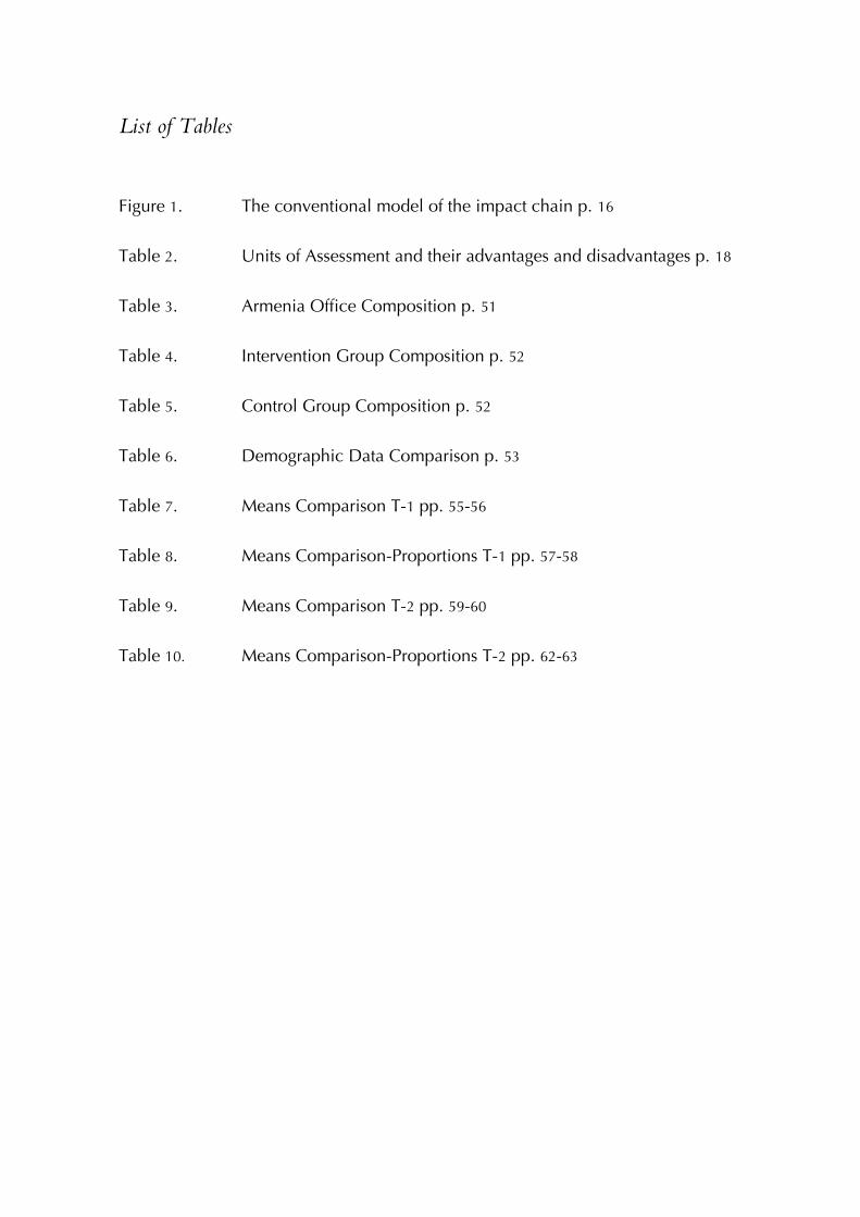
List of Tables

Figure 1. The conventional model of the impact chain p. 16

Table 2. Units of Assessment and their advantages and disadvantages p. 18

Table 3. Armenia Office Composition p. 51

Table 4. Intervention Group Composition p. 52

Table 5. Control Group Composition p. 52

Table 6. Demographic Data Comparison p. 53

Table 7. Means Comparison T-1 pp. 55-56

Table 8. Means Comparison-Proportions T-1 pp. 57-58

Table 9. Means Comparison T-2 pp. 59-60

Table 10. Means Comparison-Proportions T-2 pp. 62-63

List of Acronyms

AIMS Assessing the Impact of Microcredit Services

ANOVA Analysis of Variance

APA American Psychologist Association

ASCRA Accumulated Savings and Credit Association

BBVA Banco Bilbao Vizcaya Argentaria

CIA Central Intelligence Agency

COP Colombian Pesos

GDP Gross Domestic Product

FARC Fuerzas Armadas Revolucionarias de Colombia (Revolutionary Armed Forces of Colombia)

HEPM Household Economic Portfolio Model

HDI Human Development Index

IA Impact Assessment

IBD Inter American Development Bank

LDC Less Developed Country

MFI Micro Finance Institution

NGO Non Governmental Organization

PLA Participatory Learning and Action

ROSCA Rotating Savings and Credit Association

UN United Nations

USA United States of America

USAID United States Agency for International Development

USD United States Dollar

WWB Women's World Banking

5

1 INTRODUCTION

This paper will be based on answering a straightforward question, what is the impact of

microcredits on its beneficiaries?

In order to do this, I will present the results of a field research I did during my two

months stay in the microfinance institution Bancamia. This Colombian based microfinance

institution gave me the opportunity to work with them for two months in one of their

offices, located in the Colombian city of Armenia (department of Quindío).

The paper is structured as follows. I will first review the geographical, economic and

social context of Colombia and then the historical antecedents of microcredit. Next I will

refer to the on-going debate about microfinance in the developmental field which will be

followed by an introduction into a set of theories try to explain the existence of

microfinance and how to study their impact on the beneficiaries. Finally, I will describe the

applied methodology utilized during my field work in my research, followed by the

empirical analysis and the conclusions.

1.1 A NOTE ABOUT COLOMBIA

1.1.1 Geographical Context

Colombia is located in northern South America,

limiting with Venezuela and Panamá on the North,

and with Ecuador, Perú and Panamá on the South.

It has access to both Caribbean and Pacific Sea, and

its landscape is varied, ranging from Andes

Mountains to the Amazonian jungle and lowlands in

6

the coast. Its estimated land area is 1.038.700 m2 (cia Factbook 2012).The capital Bogotá is

also the most populated city (8.262.000 hab.), followed by Medellín (3.497.000 hab.), and

Cali (2.352.000 hab.)(Ibid.).

The city of Armenia is located 290 km

East of Bogotá, and it is the capital of the

department of Quindío. It was founded by

peasants on the 14th October 1889, with

the original name of Villa Holguín. Soon

after its foundation in 1889 the city

changed its name to Armenia Even though

the common belief is that the city was

renamed as Armenia in solidarity with the

first chapter of Armenian genocide by the

Ottomans—Hamidian Massacres of 1894–

1896—, the fact that the name was changed to Armenia soon after its foundation in 1889

makes this explanation historically incongruous. The most probable explanation was that it

was a fashion on that time in Colombia to name cities after the names of Biblical and Near

East places (Matiossián 2003).

The most tragic date in the recent history of Armenia was an earthquake 6,2 in the

Ritcher scale (usgs 2009) in 1.999 that killed about 1.000 people, and destroyed a great

part of the city, leaving about 200.000 people homeless (bbc 1999). However, Armenia

was quickly rebuilt, and now is referred as “Ciudad Milagro” (miracle city) due to its

economic growth.

1.1.2 Social and Economic Context

After a four-decade long conflict with the Revolutionary Armed Forces of Colombia

(farc), the announcement in 2012 of the release of the last political hostages (Colombia

Reports 2012) was seen as a huge step towards pacification. Violence has been decreasing

7

since 2002, but some insurgents continue to throw attacks against civilians. The total

population in Colombia according to cia Factbook (2012) is 45.239.079 (July 2012 est.),

and the life expectancy at birth is 74,79 years (Ibid.).

The economic performance of the last decade has been strong, and Real gdp grew

5,7 % in 2011 and inflation ended 2011 at 3,7 %. Unemployment is still relatively high

10,8 % in 2011—arguably due to hidden economy—and economy is still highly dependent

on oil exports (cia 2012). gdp per capita is 10.100 $ (2011 est.), which ranks the 109th in the

world (Ibid.). Its hdi (Human Development Index) in 2011 was 0,710 ranking 87th in the

world (undp 2012). Its Gini coeffient—an index that tries to quantify inequality—was 58,5

in 2005 (Ibid.).

The city of Armenia is currently the 21st most populated city of Colombia with an

estimated population of 281.013 hab. (dane 2010). The economy is based on agricultural

outputs, coffee and bananas plantation. An effort is currently being made in the whole

coffee area covering the department of Quindío, Caldas and Risaralda in order to promote

it as a touristic destination, stressing their mountainous landscape and traditional lifestyle

and branding it as the triángulo del café (coffee triangle).

1.2 HISTORICAL ANTECEDENTS OF MICROCREDIT

Although there have been some precedents of this kind of activities during the history, the

terms microcredit and microfinance did not start to be broadly used until the decade of 1970's.

What follows is a review of what the literature has considered as historical antecedents of

microfinance and a small review of its antecedents in Colombia.

8

1.2.1 Historical Antecedents of Microcredit in Developing Countries

In South Africa, Latin America and Asia, the most traditional practices that resemble

microfinance are the rosca and the ascra. In rosca (rotating savings and credit association),

each member of the group contributes with the same amount. Each time that the whole

group gathers to collect the money, a different member of the group takes all the money.

This happens usually every month. The ascra (accumulated savings and credit association)

usually has a higher number of members than rosca. The members make periodical

contributions for a determined period of time—usually a year—and after that the money

is redistributed. The ascra may also make loans with interest to people outside the group

during the year, making the funds grow even more. Their operative is somehow like a

credit cooperative, but with the difference that while cooperatives encourage permanency,

in ascra and rosca permanency is not encouraged beyond each cycle (Bouman pp. 374-

6: 1995).

In Asia, around 1880, the government of Madras (South of India), under Britannic

administration, established a credit cooperative programme inspired in German raiffesenists

cooperatives. By 1912 there were 40.000 cooperatives and by 1946 more than 9 million. In

the following years, this cooperatives lost strength, but the notion of group-lending

remained, and can be somewhat considered the seed of Grameen Bank (Morduch pp.

1573-74:1999).

Later, in 50's and 60's there was an attempt to make credit institutions in many poor

countries. Their objectives were to give poor people an alternative to the moneylenders, but

they had great losses or they were just sustained by big amounts of external donors (Adams

and Von Pischke p. 8: 1992). By 1975 the World Bank did an analysis on its Agricultural

Sector Policy Paper, concluding that more than a half of the 44 institutions analysed had a

failure ratio of 50% (World Bank 1975).

Reasons of failure were several, first of all the estimations of the investment returns

did not take in consideration the possibility of bad harvests or other unexpected

circumstances. Interest rates were too low, so there was little interest in giving small

9

credits. As they were subsidized, there was the perception that it was a donation from the

government. On the other hand, borrowers did not use the money in productive activities

or sometimes they invested in non-profitable activities (Adams and Von Pischke p. 9:

1992).

1.2.2 Historical Antecedents of Microcredit in Europe

Now I will review the antecedents of microcredit in Ireland and other European

countries, based on the analysis of Hollis and Sweetman (1998a and 1998b).

From 1720's and until 1950's in Ireland there was a network of small banks with the

aim to give credit to the poor, having its peak during 19th century, when it reached 20%

of homes in the country.

One of the precursors of microcredit practices in Ireland was the writer Jonathan

Swift—famous writer of Gulliver's Travel—who in the beginning of the 18th century

established a fund of 500 pounds for lending to poor people. This fund had a shared

guarantee mechanism between borrowers, as each lender had to present the reference of two

of his neighbours.

Later in 1747, the Musical Society of Dublin made a fund with the profit from their

concerts applying the so-called Swift system.

Due to the famine of 1822 a British committee raised an aid donor’s fund, donating up

to 300.000 pounds. There was a remainder of 55.000 at the end of the famine, so an aid a

fund was established. By 1823 the fund was authorised to earn a small interest rate,

exempted of some taxing—the stamp tax—that standard lenders had to pay. As they grew,

these funds started to operate almost as banks.

From 1840 this activity begun to decline, the reason is that population become more

urban based, so the funds lost the comparative advantage they had (first-hand information

about borrowers in rural environments).

In other European countries there are also references. In England in the 15th century

the Loan Beneficial Societies provided a kind of microfinancial service, based in that each

10

borrower had to find two cosignatories in order to get the credit. With the time it becomes

more and more difficult to have cosignatories, so these societies decreased.

But maybe the long-lasting credit cooperative experience in the world can be found

in Germany. At the beginning of the 20th century, the raiffesenists credit cooperatives

accounted more than 14.500 cooperatives and 1.400.000 members. Their members

contributed funds and earned low interests, being the profits destined to expand capital

and sometimes to social projects. Under this system, borrowers should contribute two

cosignatories in order to get the credit. There was a high refund rate, due to the high

awareness between members—as most of them knew each other’s.

Also in Italy the rural saving banks were inspired by raiffesenists credit cooperatives. They

took place in small villages having from 20 to 60 members. Each member had right to

vote, and sometimes even the obligation.

Finally in Spain their historical antecedents go back to the Montes de Piedad/Arcas de

Limosna, created in the middle ages by the Franciscan monks. These were essentially loans

with pledge for poor people. There was no interest rate, and in the case of failure the

amount was recovered with the pledge. Funds came from donations, deposits—with no

interests, but spiritual rewards—and profits. After the council of Letrán (1515), it was

allowed a small interest rate. Earlier in 1480, the town council of Gollano in Navarra

approved the first Arca de Misericordia. They were essentially loans in species—usually grain

—guaranteed with a pledge (Gutiérrez-Nieto 2005).

There was another agricultural lending procedure, the Pósito (grain warehouse

managed by the town hall where peasants could draw grain when scarcity). Later it

evolved into lending money with interests, thus losing their initial function. The decadence of

these institutions did not come until the 19th century, and mainly because of its growing

insolvency, the civil administrations took too much money from them, making them

insolvents. (Gutiérrez-Nieto 2005)

11

1.2.3 The Emergence of Modern Microfinance

The modern resurgence of microfinance—while even the word microfinance had not yet

been coined—begun in early 70’s, when scholars from several backgrounds—agriculture,

anthropology, banking, business, economics, government service, law, public policy,

religion, social work—started to learn about the dynamics of local financial markets in

development countries (Robinson p. xxx: 2001).

As stated before, the first efforts made in 50's and 60's by bankers, international donors

and policy-makers did not yield the expected results. But at the same time, some donor-

funded ngo’s were starting to identify a demand for microcredit in developing countries,

and “to develop methodologies for delivering and recovering small loans, and to begin

credit programs for the poor” (Robinson p. xxxi: 2001).

One of the first modern microfinance institutions started in 1970, as Bank Dagang Bali

opened in Bali (Indonesia). Later in 1976, Muhammad Yunus made a first experimental

loan of 1,5 $ to 43 poor people in the village of Jobra in Bangladesh. This loan was made

without collateral and interest rate, and with the aim to let this people have a small capital.

With this small amount of capital, they could pay in advance and get far better prices both

for buying and selling. This was the seed of one of the world’s best-known microfinance

institution until now, Grameen Bank. (Robinson p. xxx: 2001).

The microfinance revolution—as labelled by Robinson—then developed in the 80’s and

in the 90’s, when it “combined with a commercial approach to financial intermediation

for low income people, making financially sustainable formal sector microfinance

possible”, being the pioneers of this approach Bancosol in Bolivia and Bank Rakyat

Indonesia (Robinson 2001).

12

1.2.4 Microfinance in Colombia

In the 1950’s and 60’s, the main credit supplier to the poor population in Colombia were

public institutions of rural credit like Caja Agraria. But problems like paternalism and

corruption caused these institutions not to effectively reach the poor and later were

abandoned due to lack of self-sustainability and political support (Barona 2004). The first

mfi’s in Colombia date back to the 80’s, being 18 years the average age of the operating

institutions at the end of 2008 (Martínez 2009).

One of the pioneering initiatives was the Programa de Crédito a la Microempresa,

promoted by the Inter-American Development Bank (ibd). This programme initially started

just with the partnership of one ngo—Fundación Carvajal—but in 1984 there were already

8 institutions ascribed to this initiative. Another important effort was the creation of the

Departamento Nacional de Planificación, a public institution with the purpose of giving

continuity to the microcredit policies (Barona 2004).

While I found no reliable data in the literature concerning the performance of the

mfi’s in 90’s and early 2000’s, from 2005 and on I will take the summary from Presbitero

and Rabelloti (2012). In 2005 the Inter-American Development Bank reported that in

Colombia there were 22 mfi’s, serving more than 600.000 borrowers—being the main

operator the Fundación wwb Calí, with almost 130.000 customers. At the end of 2010 mix

Market, reported a total amount of 34 mfi’s in Colombia with about 2,1 mill. borrowers—

being the largest institution the Banco Caja Social Colombia with almost 620.000 active

borrowers and a gross loan portfolio of usd 2.400 mill. According to a study by Vision

Económica—a local business research group—microcredit in Colombia grew at a rate of 15

% each year between 2007 and 2010, when the total amount of microloans reached more

than usd 4.100 mill. (Presbitero and Rabelloti p. 5: 2012)

The latest data according to mix Market is that the number of microloans in 2011 just

grew a 2,5 % with respect to 2010, being a total of usd 4.200 mill. and that the number of

mfi’s grew to 36—being the largest ones Banco Caja Social Colombia, Bancamia and Banco

13

wwb, each one with a gross loan portfolio of usd 3.312 mill, usd 502 mill. and usd 352

mill. (mix Market 2012)

With respect to the literature concerning microfinance analyses in Colombia, I can

just cite the already mentioned by Presbitero and Rabelloti (2012), where the research is

focused in the influence of geographical distance in microfinance repayment and a case

study about Fundación wwb in Cali (Huertas 2007) that is focused on the macroeconomic

data from this institution.

Bancamia. Bancamia was founded in 2007, when the wwb Foundation in Colombia

and Cali joined efforts with bbva Foundation from Spain in order to create a mfi that could

adapt to the constant grow in demand of credit services for the microentrepeneurs. After

fulfilling all technical requirements, Bancamia opened its first branch 18th October 2008. In

its last press report on May 11th 2012, Bancamia reported having more than 500.000

customers, giving an average of 1.203 credits a day and with 161 branches all around

Colombia (Bancamia 2012a), reporting profits of 16.110 mill cop (Colombian Pesos) in

2010 and 36.103 cop in 2011 (Bancamia 2012b).

14

2 THEORETICAL FRAMEWORK

Microfinance popularity has increasingly been growing in last two decades, and the topic

has recently reached the public opinion. One of the facts that drew more attention from

the global audience was in 2006 when Mohammed Yunnus and the Grameen Bank were

awarded with the Nobel Peace Prize due to “their efforts to create economic and social

development from below” (Nobel Prize 2006). But at the same time, critics to

microfinance also started to reach the public through the media (Bunting 2010). In many

cases these criticisms were targeting Grameen Bank with the argument that microcredits

did not really help the poor—but on the contrary, they could make poor people fall into a

spiral of over-indebtedness (Bajaj 2011)—and even portraying cases where physical threat was

used in order to make the borrowers to pay (Malik 2010). Even an accusation of Grameen

Bank diverting funds from Norwegian cooperation reached the media (bbc 2010) and had

to be refuted by the Norwegian Ministry of Foreign Affairs (norad 2010)

Meanwhile, microfinance has become one of the most important tools of

development policies. According to the un, and as stated in the un Millennium Summit in

September 2000, microfinance should be a key strategy to achieve the Millenium

Development Goals. In order to support this thesis, some authors give examples where

microfinance has been empirically proved to eradicate poverty, promote children

education, improve health for women and children, empowering women and targeting

the poorest (Morduch et al. 2003). On the other hand, other authors prevent that mfi’s does

not always target the poor and the poorest but they often target less poor customers (Hulme

2000a)

15

2.1 WHY MICROFINANCE?

“Lack of access to credit is generally seen as one of the main reasons why many people in

developing economies remain poor” (Hermes and Lensink 2007).

2.1.1 Definition of Microcredit

Even today the discussion about what defines a microcredit is still going on. Some definitions

point to their lending mechanisms as one of its most characteristic features, “group lending is

not the only mechanism that differentiates microfinance contracts from standard loan

contracts. The programs [...] also use dynamic incentives, regular repayment schedules,

and collateral substitutes to help maintain high repayment rates” (Morduch p. 11: 1999).

Other definitions, like the one agreed during the Microfinance Summit in 1997 put the stress

into poorness and self-employment, as microcredits are defined as “programmes extend small

loans to very poor people for self-employment projects that generate income, allowing

them to care for themselves and their families” (Srinivas, 1997).

Even though, a universal definition would hardly fit the diversity of microfinance

practices all around the world, from the western to the less developed countries. An example

in Europe is the recently approved European Code of Good Conduct for Microcredit Provision

(European Commission 2011), that for example has defined its scope as “primarily

designed to cover non-bank microcredit providers which provide loans of up to 25.000 €

to micro-entrepreneurs” (European Commission p.10: 2011). But other definitions not so

bounded geographically already defined the maximum amount of a microcredit in no

more than 1.000 $ (Microfinance Bulletin p.6: 1997).

2.1.2 Formal vs. Informal Sector

16

Given the multiplicity of definitions of microcredit, in this paper I am going to depart

from the notion that microcredit is one tool in order to give the poor an alternative to the

informal sector. This is almost universally accepted as being one of the main objectives of

microfinance (Morduch 1999; Gutiérrez-Nieto et al. 2004; Helms 2006; Morvant-Roux

2009). The existence of microfinance is often justified as a way to give an alternative to

people that are excluded from the traditional banking sector and just have the informal sector

in order to attend their financial necessities. The differences between both formal and

informal sector are often blurry, and they might be characterised as a continuum ranging

from “moneylenders, community savings clubs, deposit collectors and agricultural input

providers traders and processors” (Helms p. 35: 2006) in one side to private and public

banks in the other. In the middle of the spectrum there are “member-owned institutions,

ngo's and nonbank financial institutions” (Ibid.).

Researchers studying the profile of microcredit customers have described them as

being from moderately poor and vulnerable non-poor households—that is being more or less

above and below the poverty level—and also with some customers from extreme-poor

households (Helms p. 20: 2006). While some programs explicitly targeting poorer

segments of the population generally have a greater percentage of clients from extreme-poor

households, destitute households are outside the reach of microfinance programs (Helms p.

20: 2006).

I will first review the approaches that have been used to explain the interactions

between the formal and informal forms of credit. There are two theoretical approaches that

explain the coexistence of both financial sectors, one is the residual approach and the other

one is defined as the approach “whereby the most effective cost of borrowing is thought

to be used” (Boucher et al. 2007 as in Morvant-Roux 2009).

In the first one—the residual approach—the informal sector has a residual role, as it just

receives the applications that the formal sector was not able to fulfil—the so-called spillover

demand (Conning 1999 as in Morvant-Roux 2009). This approach explains the existence

of informal credit markets either as consequence of a monopolistic position—when the

informal market is the only source of credit available—or as a part of a perfect credit

market with perfect competition—when they coexist with formal forms or credit (Hoff

17

and Stiglitz 1990). This assumptions of complete markets and perfect information, “if

questionable in more developed economies, are clearly irrelevant in ldc’s” (Stiglitz p. 257:

1986), that is, where most of the microfinance activity takes part.

On the other hand, the second approach takes the coexistence of the informal and

formal sectors as a result of a rational decision of the borrower. This approach, in

opposition of the residual approach, is based in the imperfect information paradigm, which

stresses the importance of the asymmetries of information, that is, when the borrower and the

lender have access to different (asymmetric) amounts of information in order to evaluate

the risk of each transaction (Hoff and Stiglitz, 1990).

Under this approach, the borrower evaluates both formal and informal alternatives in

terms of cost of borrowing (related to interests, collateral, transaction costs, etc.) and risk

evaluation (related to for example the risks of undertaking a formal contract). If these

prove to be weaker in the informal sector, this is where the borrower will first apply

(Morvant-Roux p. 13: 2009). In order to overcome information asymmetries, moneylenders

in the informal sector will sometimes resort to the use of enforcement mechanisms, like for

example the use of interlinkages with other markets—e.g., when the moneylender takes

also the role of supplier in a rural environment—or kinship and/or geographical ties.

These enforcement mechanisms could determine which credits will have preference to be

paid by a borrower with both credits in the formal and informal market—that is, which

credits are treated as senior debt and which are treated as junior debt (Hoff and Stiglitz,

1990).In this paper I will take this second approach, which is based on the imperfect

information paradigm.

2.1.3 The Imperfect Information Paradigm

This paradigm departs from the assumption that there are differences in the information

available between both sides (borrower and lender), so an analysis should take in

consideration these differences and to explicitly state the point of view taken. This idea

was first developed by George Akerlof in the article “The Markets for Lemons” (1970),

18

where he described the difference of information between buyers and sellers in the

American used cars market and in the insurance market. It was later developed by Joseph

Stiglitz, who first applied it in order to explain the functioning of credit markets (Stiglitz

and Weiss 1981), and later used this model in order to explain the success of some

microfinance institutions in order to discriminate between low-risk and high-risk customers

(Stiglitz 1990).

This approach finds unrealistic the assumption of a world with perfect and costless

information where the bank would stipulate precisely all the actions which the borrower

could undertake—and which might affect the return to the loan (Stiglitz and Weiss pp.

393-394: 1981). As opposed to that, under the imperfect information paradigm, “the bank is

not able to directly control all the actions of the borrower; therefore, it will formulate the

terms of the loan contract in a manner designed to induce the borrower to take actions

which are in the interest of the bank, as well as to attract low risk borrowers” (Ibid.).

Behind the imperfect information paradigm lays the theory of asymmetric information. This

theory is based in the fact that information is different to any other commodity, as each

piece of information has to be new to the receptor in order to be valuable. So markets of

information are characterized by imperfections of information about what is being

purchased (Stiglitz 2000). This is related with the problems of moral hazard and adverse

selection.

Moral hazard is related to a hidden action—an action (or omission) that is hidden for

one of the parts of the economic relation—and occurs when the party insulated from risk

behaves differently than it would behave if it were fully exposed to the risk. In banking,

this would happen if, for example, the lender does not use the money of the credit in a

productive and that worsens the probabilities of paying it back. Adverse selection is a market

process in which as a result of the asymmetric information—that is, both parts of the

transaction having different information—the bad product or customer is more likely to be

selected. In banking this would mean that for example with a too high interest rate a bank

would only attract the riskier projects.

The problem of adverse selection can be overcome by self-selection, meaning this “the

process by which individuals reveal information about themselves through the choices that

19

they make” (Stiglitz p. 1450: 2000). The problem of moral hazard is, overcome with

monitoring or screening and with the use of incentives (Stiglitz p. 1454: 2000).

2.1.3.1 The Imperfect Information Paradigm: Joint Liability vs. Individual Liability

One of the characteristics of microfinance is creation of mechanisms in order to overcome

the asymmetries of information.

One of the most studied is joint liability group lending, that uses groups of borrowers

instead of individuals to give the credit. If one of the members of a group fails to pay back,

the rest of the members have to contribute in order to ensure the full repayment. Joint

liability group lending “stimulates screening, monitoring and enforcement of contracts among

borrowers, reducing or erasing the agency costs of the lender” (Hermes and Lensink

2007), due to social ties and geographical proximity. This is also supported by theoretical

models by Stiglitz (1990), Banerjee et al. (1994 as in Hermes and Lensink 2007), or

Armendáriz de Aghion (1999), and by several empirical studies as shown in Hermes and

Lensik (2007). Another mechanism that works under group lending is the creation of social

capital and social ties between the customers, as shown in Cassar et al. (2007).

But in recent years, individual liability is having a growing importance as many mfi’s

are shifting or taking this mechanism in account (Giné and Karlan p. 5: 2010). With this

method, moral hazard would be avoided with the use of reputation (Stiglitz 2000), and the

use of incentives like the progressive access to larger amounts of credit, as “new borrowers

are provided small loans and allowed to increase loan sizes by demonstrating prompt

repayment” (Robinson 2001). Also, some of the drawbacks of group lending joint liability—

like tensions within the group, free rider problem, higher costs for better customers or lack

of adaptability to demand—would be overcome with this method (Giné and Karlan pp. 5-

6: 2010).

As a summary, under the imperfect information paradigm, the lending activity entails

five components: “(a) the exchange of consumption today for consumption in a later

period, (b) insurance against default risk, (c)information acquisition regarding the

20

characteristics of loan applicants (this is the screening problem) (d) measures to ensure that

borrowers take those actions that make repayment most likely (this is the incentives

problem); and (e) enforcement actions to increase the likelihood of repayment by borrowers

who are able to do so” (Hoff and Stiglitz p. 37: 1990).

2.2 CONCEPTUAL FRAMEWORK

So far I have argued that in this study I consider microcredits as an alternative to the

informal sector—while coexisting with it at the same time—in a non-perfect credit market

characterized by the existence of asymmetries of information. I will now review the

theoretical basis of the different methodologies for the impact assessment (ia) of

microfinance.

Before deciding which methodological approach a microfinance ia wants to adopt,

the researcher has to face with the choice of a conceptual framework. This choice is

sometimes explicitly stated (Khandker 1998; Sebstad, Neill, Barnes and Chen 1995;

Schuler and Hashemi 1994 as in Hulme p. 82: 2000b), but in many microfinance ia’s is

just implicitly taken for granted.

I will start by explaining the three main elements of a conceptual framework according

to Hulme (p. 82: 2000b):

“—a model of the impact chain that the study is to examine,

—the specification of the unit(s), or levels, at which impacts are assessed, and

—the specification of the types of impact that are to be assessed.”

2.2.1 The Impact Chain

The model of impact chain is depicted in figure 1. The impact chain consists in a programme

that modifies the behaviour of an agent (beneficiary) and modifies the outcome of the

21

beneficiary and/or other agents. But we have to take care with this explanation, as it can

just be taken a simplification in order to explain how the model works.

Reality is often more complex, as in many cases an effect may at the same time

becomes a cause, “a more detailed conceptualization would present a complex set of links

as each effect becomes a cause in its own right generating further effects” (Hulme p. 82:

2000b). One of the main difficulties when establishing an impact chain is endogeneity. This

problem “occurs when changes in the explanatory (independent) variables are caused in

part by the dependent variable” (Gaile and Foster p. 17: 1996).

Under this model, a microfinance ia measures “the difference in the values of key

variables between the outcomes on agents (individuals, enterprises, households,

populations, policymakers, etc.) which have experienced an intervention against the values

of those variables that would have occurred had there been no intervention” (Hulme p.

82: 2000b).

The other main difficulty when analysing an impact chain is the fact that an agent

cannot experience and not experience the same intervention at the same time. This is one of

22

the main methodological difficulties that any impact analysis has to overcome, as we will

see later in this research.

2.2.2 Units of Assessment

Once the chain of impact has been designed, the next step in a microfinance ia is the

choice of the units (levels) of assessment that the research will take in consideration. The

literature has reviewed impact assessment from several different focuses, ranging from the

individual level (e.g., Goetz and Sen Gupta 1996 and Peace and 1994 as in Hulme p. 82:

2000b) to a combination of several levels, like in the Household Economic Portfolio Model

(Chen and Dunn 1996).

A summary of the advantages and disadvantages of each unit of assessment is made in

table 2, taken from Hulme (p. 83: 2000b).

23

TABLE 2 —UNITS OF ASSESSMENT AND THEIR ADVANTAGES AND DISADVANTAGES

Unit Advantages Disadvantages

Individual —Easily defined and identified —Most interventions have impacts

beyond the individual—Difficulties of disaggregating group

impacts and impacts on relationsEnterprise —Availability of analytical tools

(profitability, return on investment,

etc)

—Definition and identification is difficult

in microenterprises

—Much microfinance is used for other

enterprises and/or consumption—Links between enterprise performance

and livelihoods need careful validationHousehold —Relatively easily defined and

identified

—Sometimes exact membership difficult

to gauge—Permits an appreciation of

livelihood impacts

—The assumption that what is good for a

household in aggregate is good for all of its

members individually is often invalid—Permits an appreciation of

interlinkages of different enterprises

and consumption

Community —Permits major externalities of

interventions to be captured

—Quantitative data is difficult to gather

—Definition of its boundary is arbitrary

Institutional —Availability of data impacts —How valid are inferences about the

outcomes produced by institutional

activity?—Availability of analytical tools

(profitability, SDIs, transaction costs)Household economic

portfolio, (i.e.

household, enterprise,

individual and

community)

—Comprehensive coverage of

impacts

—Appreciation of linkages between

different units

—Complexity

—High costs

—Demands sophisticated analytical skills

—Time consuming

Source: Hulme (p. 82: 2000b)

24

Focusing on the disadvantages, all of the pure approaches have some conceptual

drawbacks that could limit or even discredit the validity of the analysis, while the

Household Economic Portfolio can be seen as a mixture of all the approaches trying to

overcome their limitations. On the other hand, the Household Economic Portfolio demands

more resources in order to implement it. This can have the side effect that impact analysis

with limited resources may risk “sacrificing depth for breadth of coverage of possible

impacts” (Hulme p. 82: 2000b).

2.2.3 Types of Impact

In each of the units analysed, the choice of variables that can be used to assess impact is

almost infinite. But in order to be useful, these variables must be “able to be defined with

precision and must be measurable” (Hulme p. 83: 2000b). Some of the most used variables

in the literature are economical—like income, level of assets or debt—but the use of social or

gender perspectives in the impact analysis has broadened the choice of variables (Hulme p.

83: 2000b).

A comprehensive list of variables used in impact analysis, covering variables relating

to Education, Household, Assets/Wealth, Land, Program, Credit/Loan Information, Participation,

Village Attributes, Income, Gender, Labour, Enterprise, Consumption and Impact can be found

in Gaille and Foster (Annex 1: 1996).

25

2.3 APPLICATION OF THE CONCEPTUAL

FRAMEWORK

Some of the most widely used criteria when trying to measure the success of a

microfinance programme are: “the client households’ increased overall well-being; or

clients’ business success; or the community’s improvement; or the program’s financial

viability (e.g., payback/default rates)” (Gaile and Foster p. 3: 1996).

As I have pointed before, in order to choose the criteria for a microfinance ia, first I

have to choose which point of view to take in it regarding the chain of impact. Given the

complexity of characterising an impact chain, and the difficulty in order to “separate

project and non-project influences” (Mosley p. 3: 1997), Hulme characterization of two

different schools of thought in microfinance evaluation is based “with regard to which

link(s) in the chain to focus on” (Hulme p. 82: 2000b). Intermediary school focuses in the

beginning of the impact chain—that is, in the lender side—while intended beneficiary school

tries to go as down of the impact chain as possible—that is, focusing in the borrower side.

2.3.1 The Intermediary School

The first approach—the intermediary school—is taken from the perspective of the

borrower/borrowing institution. The roots of this approach go back to the Ohio State

University School analyses of rural finance, focusing mainly on two variables: the

institutional outreach and the institutional sustainability of the programme.

According to this school, if these two impacts have taken place, an intervention is

judged as beneficial. “This is based on the assumption that such institutional impacts

extend the choices of people looking for credit and savings services and that this extension

of choice ultimately leads to improved microenterprise performance and household

economic security” (Hulme p. 82: 2000b). Although this assumption can be supported by

some theoretical models, it requires further assumptions regarding perfect competition

26

which falls outside of the imperfect information paradigm—and it has been empirically

proved invalid in a number of experiences (Ibid.).

The duality between institutional outreach and institutional sustainability also gives rise to

two different—and in some way opposed—approaches in the microfinance world,

labelling them as the financial systems approach and the poverty lending approach (Robinson

2001). Even though both approaches agree in the same goal—to serve as many poor

people as possible—, they differ in the means that should be used to reach it (Hermes and

Lensink 2007). While the financial systems approach puts the stress in the financial

sustainability of microfinance programs, the poverty lending approach stresses the

importance of using credit—even with subsidised rates—in order to overcome poverty.

It should be noted however the relevance of the financial systems approach in the

analysis of the viability of the mfi’s with economic criteria, especially their viability and/or

their self-sustainability (Morduch 1999, Gutiérrez-Nieto et al. 2004, Gutiérrez Nieto et al.

2011). Questions arising in this approach are if a mfi should aim to be run without

subsidies even at the expense of raising the interests up to 40%, or if microfinance

programmes justify their subsidies when reaching the outreached (Morduch p. 3: 1999).

This is related as well with the ongoing discussion in development studies about if donors

should aim to the self-sustainability of the agents, regardless of considerations about if it is

possible to reach the poorest and be self-sustainable at the same time.

2.3.2 The Intended Beneficiary School

The alternative point of view to the intermediary school is concerned with the analysis of

the impact of microcredit programmes in the life of their beneficiaries, that is, from the

point of view of the borrower. This focus, is the intended beneficiary school that “building on

the ideas of conventional evaluation, seeks to get as far down the impact chain as is

feasible (in terms of budgets and techniques) and to assess the impact on intended

beneficiaries (individuals or households)” (Hulme p. 82: 2000b).

27

When taking this approach although and trying to focus “as down in the chain as

feasible “(Ibid.), the choice of a unit of assessment will determine the conceptual model

used. This shall be made taking in consideration the results that the impact evaluation

wants to reach, but also the restrictions of the researcher (physical, monetary, etc.)

Given the previously stated focus in the imperfect information paradigm, and as the

intermediary school approach departs from some assumptions unsupported by this paradigm,

in this research I am taking the point of view of the intended beneficiary school. This means

that the research focuses in the end of the impact chain, that is, in the—positive or

negative—impact of the microcredit programme to the beneficiary. This focus makes less

a priori suppositions about the impact chain and it is generally better in determining the

who and how, although more demanding both methodologically and in costs (Hulme p. 82:

2000b).

So after choosing the level of the chain of impact I am going to focus on, the next

step will be choosing the units/levels of assessment that the research is going to take in

consideration.

2.4 MODEL OF THE IMPACT ANALYSIS

As previously exposed in Figure 1—when talking about the pure approaches in relation

with their units/levels of assessment—“a focus purely on the individual or the enterprise has

such drawbacks that they could be viewed as discredited” (Hulme p. 83: 2000b). Given

the conceptual advantages (it covers several levels of assessment and the relation between

those levels), in this research I will take the approach of the Household Economic Portfolio

Model (hepm). This model also incorporates the role of risk, which also fits under the

imperfect information paradigm.

In order to contextualize the hepm I will first make a review of its antecedents and

then I will speak about its main features and applications.

When analysing the antecedents of the hepm, the two major developments through

the evolution of household models are the integration of the production and consumption

28

models and the disaggregation of the household in order to “reveal the role of individual

preferences, resources, and bargaining power in intrahousehold decision making” (Chen

and Dunn p. 12: 1996).

In order to present that development, I am going to make a historical review of

different economic theories and the units of analysis—in analogy of the units of assessment

—that they have used. For that I will follow the schema described in Household Economic

Portfolios (Chen and Dunn 1996). First I will review the different definitions of household

and its relations with other levels, and then I will introduce different economic models

and theories of household decision making.

The first criteria in order to classify the models will be whether they take in account

or not bargaining power and decision making into the household. According to this criterion

will differentiate between models dealing with household level analysis, and then the ones

dealing with intrahousehold analysis. Another criterion used will be the internal division

within the household made in some economic models. While some of the models

distinguish between the commodity and non-commodity sector (that is, between the

production of market and consumption goods), others make an internal gender-based

division in the household—that is, they divide the household in male and female. Both

divisions may even interact in some models. The last criterion used will be resource

allocation, where it is distinguished between pooled and non-pooled models.

Finally I will also review how different how different models/theories have

approached the role of risk.

2.4.1 Definition of Household

The definition of household has been approached by several social sciences. Anthropology

has centred its view in the relationship between household and family, while economy has

centred its analysis in defining the household in relation with production and

consumption. In both disciplines, feminist scholars have also looked at it focusing in a

gender approach, that is, in the relation between men and women (Chen and Dunn, p. 3:

1996).

29

The interaction of these three points of view has produced three main developments

in the definition of the household. The first one, influenced by feminist perspective that

has conceptualized households “as the site of women's oppression and as the locus of

conflicts of interest between women and men” (Moore 1994 as in Chen and Dunn, p. 3:

1996). This marked a shift from models that implicitly assumed altruism and cooperation

in any case to models that “include the possibility of negotiation, bargaining, and (even)

conflict” (Chen and Dunn, p. 13: 1996).

The second development is influenced by the anthropologist perspective where the

concept and structure of the household “both produce and are produced by larger-scale

cultural, economic and political processes" (Moore 1994 as in Chen and Dunn, p. 3:

1996). This approach has caused “a shift from the analysis of the household as a bounded

unit towards a view which stresses its permeability” (Ibid.).

The third development, also highly influenced by the anthropologist approach, has

been the recognition of the variability of the household between different societies or

even into the same society. This has yielded a definition of household as “a family or

kinship unit (e.g., the conjugal family) or as those who share a common residence or as

those who share a joint function such as consumption, production, investment or

ownership” (Chen and Dunn, p. 3: 1996). It should be taken in consideration that the

three elements of this definition may or may not coincide at the same time.

2.4.2 Household Level Analysis

Two main characteristics will differ in these models. First, the way they treat consumption

and production function, and then their assumptions about the relations between the

household and credit, labour and land market (perfect or imperfect competition and/or

information).

Neoclassic theory takes two units of analysis, consumers and firms. The consumer can

be either an individual or a household. However in this theory both units are treated

independently. So when analysing the theory of consumption, the household or individual is

the subject of analysis, and tries to maximize its utility finding the optimal combination of

30

goods and leisure. The idea that the household or individual have a utility function and

the assumption that they try to maximize it are the basis of this theory.

But when analysing the theory of production, the firm is the only subject of analysis, and

it tries to optimize the production function, that is the combination between inputs and

outputs, in order to maximize its profit. Some key assumptions are that the availability of

inputs as well as the amount of outputs the firm can sell are considered unlimited. So in

order to explain the economic behaviour of individuals or household, “neoclassical

consumer theory lacks an explicit linkage to the household's production activities” (Chen

and Dunn, p. 13: 1996). In the core of the model is also the existence of complete markets

and perfect information.

A model that tries to combine both elements of the neoclassic theory—both

consumption and production—and introduces the division between commodity and non-

commodity work is the Chayanov model. This model was developed by Alexander

Chayanov in 1923 in order to study the economy of peasant households in Russia

(Harrison 1975).

Under this model, “the household seeks to maximize its utility, where utility is

derived from the consumption of goods produced on the farm, purchased goods, and

leisure” (Chen and Dunn, p. 14: 1996). This model provides a link between production

and consumption theory, as it combines utility maximization and the production function.

The main assumptions of this model are that “the household does not have access to wage

labour, and that the household has unlimited access to land” (Chen and Dunn, p. 14:

1996).

Another model that departs from the neoclassic theory of consumption is the new home

economic model, proposed by Becker (1965) under the framework of new home economics.

This model explicitly takes the household as the unit of its analysis, being these households

“both producing units and utility maximizers” (Becker p. 495: 1965). In order to create a

link between production and consumption, the model introduced the concept of the so

called Z-goods or Z-commodities. These goods are created by the members of the household

by combining their time and human capital with purchased goods, creating then the Z-

goods. These goods become part of the utility function of the household, creating a link

31

between utility maximization and the problem of time allocation between the commodity

and the non-commodity sector.

Finally, the farm household model was first proposed by Barnum and Squire (1979) in

order to analyse agricultural households, but it is possible to apply to non-agricultural

households as well. The main contribution of this models is that it distinguishes between

paid (wage) work and work in an own enterprise, as well as between goods produced for

consumption and for production. Under this model, the household tries to optimize time

allocation between work on an own enterprise, wage work and leisure, assuming a

household in complete factor, product markets and credit markets.

32

2.4.3 Intrahousehold Level Analysis

Up to now the models described make the assumption of altruism between the household,

so there is just one a utility function for all the members of the household, and a benevolent

dictator is assumed to reconcile the members’ individual interests when they collide,

making sure that they pursue the common interest.

In contrast with the assumptions of household models, the intrahousehold models

“depart from the household models’ assumptions of joint household utility functions and

altruism and replace them with conflict, bargaining, and unequal power relationships

between the husband and wife” (Chen and Dunn p. 17: 1996). This establishes a

framework to introduce the division of the household between husband and wife, in

order to analyse differences in “time allocation, expenditure patterns, access to resources,

and enterprise choice” (Ibid.).

2.4.3.1 Intrahousehold Level Analysis: Pooled Models

In the intrahousehold analysis we can distinguish between pooled and non-pooled models.

Pooled income models consider that husband and wife share common (pooled) resources.

But instead of having a single (joint) utility function, they use separate utility functions for

male and female (Manser and Brown 1980, McElroy and Horney 1981, Lundberg and

Pollak 1993 as in Chen and Dunn p. 17: 1996). One of the basic assumptions is that men

and women will cooperate until the utility of the marital arrangement exceed the utilities

they could get outside the arrangement, being this a fallback position1. This fallback position

can also reflect consequences of the power inside the household. “Examples of variables

that affect the fall back positions include conditions in the labor market, conditions in

marriage markets, rules governing property rights, laws governing divorce, and physical,

1 That is, the point from where cooperation ceases from being beneficial.

33

financial, and human capital assets held by the individual marriage partners” (Chen and

Dunn p. 18: 1996).

2.4.3.2 Intrahousehold Level Analysis: Non-Pooled Models

In opposition, the non pooled income models keep on assuming that husband and wife have

different utility function, but also separated non shared income. In the the general collective

bargaining model (Chiappori 1992), the different members of the household have separate

labour and non-labour income, but also a share agreement. Changes in the income of any of

the members will not affect other members’ utility maximization as long as it doesn’t

change the outcome of the share agreement.

The conjugal contracts model (Carter and Katz 1996) also incorporates the possibility of

collaborating when producing Z-goods. Bargaining is reflected in this model by the exit

(meaning the indirect utility the individual might gain dissolving and/or leaving the

household) or voice (referring to the degree that both partners can influence and/or bargain

in the determination of time allocation) options (Ibid.). Finally, in the reciprocal claims

model and the separate spheres model the household is divided in gender-specific economies

where both husband and wife may cooperate in determining optimal levels of income

transfers, but when it comes to resource allocation, they each will decide their optimal

choice according to their individual resource constraints, but also taking in account

partners’ changes in resource allocation (Katz 1992, Lundberg and Pollak 1992 as in Chen

and Dunn p. 18: 1996).

2.4.4 Risk and Coping Response Models

In addition to that, some models also take in consideration the role of risk in the

household. Literature concerning household economic models define risk either “as the

34

variance in outcomes, such as variance in profits or income, or it is defined as the

probability of a negative outcome (a loss).” (Chen and Dunn p. 18: 1996) If a household is

in the edge of survival, its risk aversion may be higher than the one of a household with

more economic security, as in the first case a negative outcome could translate with a

failure to survive. The following description will take in consideration risk primarily as

associated “with the source of livelihood, of income, or (simply) of food” (Ibid.), and it

will distinguish between models of risk per se and models of responses to risk.

2.4.4.1 Risk and Coping Response Models: Models of risk

About risk per se, the most common distinction is drawn between recurrent—more

predictable, like seasonality—and periodic—less predictable and more severe, like floods—

(Morduch 1997), and associated with that two there are two other key dimensions, one

temporal—the temporal length of the crisis2 period—and one spatial—the geographical

range of the crisis.

Taking in account the nature of these risks—mainly predictability and periodicity—

households take different precautionary and response strategies (Morduch 1997). Some types

of precautionary strategies are the diversification of income and/or livelihoods, the

accumulation of assets, and the “social investments in reciprocal or redistributive systems

among households” (Chen 1991; Huss-Ashmore 1988; Shipton 1990 as in Chen and

Dunn p. 18: 1996), like norms concerning reciprocity and caring for vulnerable members

among marriage, lineage or kinship groups (Chen and Dunn p. 20: 1996).

2.4.4.2 Risk and Coping Response Models: Models of Coping Strategies

The response strategies typically referred by household models depend on the stage of the

crisis—early, middle, and late—being from low to high severity depending on the

response measures involved, and some models also include also a recovery phase (Ibid.). In

2 Understood as a collective negative shock (Dercon 2002)

35

summary, the literature consider four important dimensions in coping strategies, that is

adjustments in work, consumption assets and other social relationships, the level at which

the strategy is negotiated (household, community, etc.), the degree of reversibility of the

strategy and finally the sequence or timing of household strategies (Chen 1991 as in Chen

and Dunn p. 20: 1996).

2.4.5 The Household Economic Portfolio Model

The hepm (household economic portfolio model) was developed in order to assess the design of

the usaid project on Assessing the Impact of Microcredit Services—aims (Sebstad et al.

1996), that is was designed specifically for microcredit ia.

This model incorporates some features from previous models, and integrates it. It

includes several divisions into the household, like commodity vs. non commodity—market vs.

nonmarket spheres of production—and gender-based—male vs. female domains of

resources, activities, and power, as well as other socially defined hierarchies—(Chen and

Dunn p. ix: 1996). In relation with the duality of pooled vs. non pooled models, the hepm

does not make any assumption about if the resources are held jointly or not. It just

recognizes a wide variety of “possible intrahousehold arrangements, including pooled-to-

non pooled income, joint-to-separate preferences, cooperative-to-conflictual bargaining,

and joint-to-separate allocation of time and resources” (Chen and Dunn p. ix: 1996).

Its units of assessment are the individual level—“individual member of the household,

and the intrahousehold dynamics between members” (Ibid.)—, the household as a whole at

an aggregate level, and finally the microenterprise and the community level—regarding

“interactions of the household, its members and the wider social and economic

environment” (Chen and Dunn p. 23: 1996).

The household economic portfolio is then defined as “a) the set of household resources, b)

the set of household activities, and c) the circular flow of interaction between household

resources and household activities” (Chen and Dunn p. 23: 1996).

The typology of the resources available for the household can be human—like time,

36

labor and skills—physical, and financial. About household activities, they can take form of

consumption, investment or production activities—being the production either wage work,

income generating activities and household maintenance. The link between activities and

resources is that while resources support the developing of activities, the output of these

activities goes as well to the pool of resources.

However, the model does make some assumption relating cooperation, bargaining

and/or conflict inside the household. The members of the household may have separate

preferences, as well as separate resources and budget restrictions, so they may take

individual as well as joint decisions and/or activities. Individuals may or may not choose

to cooperate in certain situations. And finally, the strategies of the individuals reflect

differences in power due to asymmetries in access to resources, and in their social roles

and relationships.

2.4.5.1 The Household Economic Portfolio Model: The Portfolio System

The process in which the household rearranges its mix of resources, labour and activities is

described as a portfolio system. This can be defined as “the mix of strategies, both individual

and collective, developed or drawn upon by a household over a given period of time for

economic and social objectives” (Chen and Dunn p. 26: 1996).

This system is based in several assumptions. First is the existence of individual—and

sometimes competing—preferences between the members of the household. Second is the

existence of bargaining and conflicts within the household. Third is the assumption that

the members of the household may or may not cooperate in any decision. And finally that

bargaining power reflects the access to resources.

This gives raise to several patterns of the activities of the members within the

household. This is illustrated as man and woman may have separate, parallel activities (e.g.,

one in the commodity and the other in the non-commodity market), or perform integrated

activities (e.g., joint agricultural production), or even substitutable activities (e.g., man

withdrawing for agriculture to pursue an alternative employment, leaving all tasks for

women).

37

Some dimensions of the portfolio system have special relevance when analysing the

impact of a microcredit programme. Gender dimension is given a great importance, as

women are considered more likely of moving between different sectors of production—

commodity and non-commodity—and to have different preferences, constraints and/or

resources than men. The risk dimension is also considered, as poorer and richer households

manage risk differently and have different risk aversions. Finally, nonmarket modes of

production like subsistence production—in agrarian communities, time spend working in

the household, family labour—or subsistence activities—like time spent on food, fuel or

water collection—are also considered (Chen and Dunn p. 27: 1996).

2.4.5.2 The Household Economic Portfolio Model: Applications of the hepm

The typology of portfolio systems in a specific area is characterised by the hepm in a

continuum that goes from the poorest to the richest households. The poorest ones are

expected to pursue short-term survival objectives, mainly through the diversification and

intensification of labour activities. Apart from the objective of survival objectives, they

would also save for contingencies, in order to be able to response crisis avoiding a forced

sale of assets. On the contrary, richest households will be expected to pursue long term

mobility through diversification of assets and investments, as well as other objectives like

increased power income or status (Chen and Dunn p. 27: 1996).

Thus, the households in the middle term between the poorest and the richest, will

pursue stability and security objectives, but will also try to minimize risks when looking

ahead for economic and social mobility. “The calculation of trade-offs between status, risk

aversion, and income or between consumption, savings, and investment would most likely

be less straightforward than for those households at either end of the continuum” (Chen

and Dunn p. 28: 1996). The key distinctions between all the households in these three

points are according to this model, the level of income or welfare of the household, the

approach to risk management and the degree of diversity of activities or strategies (Chen

and Dunn p. 28: 1996).

So at this point, the hepm identifies the households with lower levels of economic

38

security with those with the smaller set of resources, including fewer physical and financial

resources. These households would have to support mainly through their available labour,

with the implication of having less capacity to support household activities, which may

imply lower consumption and fewer production and investment activities (Ibid.).

This suggests two possible indicators of the security of the household “1) the income

and other additions to resources flowing from the household activities to the household

resource base (a flow measure) and 2) the value of household resources (a stock measure)”

(Ibid.).

About the role of credits in the households, according to the hepm, the credit when

received creates an addition in resources available. This extra resources may be allocated to

just one or to all of the household activities. If the credit was received in a previous

period, it will be also take resources out of the household in the form of debt repayment,

but if the credit was used in production or investment activities, it may also have increased

the flow of resources of the household, increasing repayment capacity. Another use of the

credit would be to smooth consumption in a period when the resources of the household

are low, but on the other hand this does not directly increase repayment capacity of the

household. (Chen and Dunn p. 29: 1996)

Another implication of the hepm will affect intrahousehold behaviour. Given the

assumptions made about cooperation, bargaining and/or conflict, when the credit is received,

the individual who controls it would determine the allocation of the extra resources

between different household activities, and may choose to invest in their separate activities

or in the joint activities of the household. According to hepm, when the preferences or

constraints of the members of the household are different, individuals may take irrational

decisions from the household point of view, like for example investing in a less-

productive enterprise than other, but over which they have control (Ibid.).

2.4.5.3 The Household Economic Portfolio Model: Proposed Hypothesis

As a conclusion to the model, the authors recommend three sets of hypotheses. The first

group is concerned with “the impacts of microenterprise services on household income

39

and the portfolio of activities that generate income” (Chen and Dunn p. 33: 1996):

— H-1: Participation in microenterprise services leads to an increase in

household income.

— H-2: Participation in microenterprise services leads to increased

diversification in the set of production activities.

— H-3: Participation in microenterprise services leads to an increase in the

reliance of the household on high-return production activities.

The second group of hypotheses are “concerned with the impacts of microenterprise

services on the investments of the household [...] and focus on the set of household

resources”:

— H-4: Participation in microenterprise services leads to an increase in key

physical assets.

— H-5: Participation in microenterprise services leads to an increase in

savings.

— H-6: Participation in microenterprise services leads to an increase in

expenditures on the education and training of household members.

Finally, it makes two hypotheses at the individual level:

— I-1: Participation in microenterprise services leads to increased control by

the client over resources within the household.

— I-2: Participation in microenterprise services leads to an increase in the

amount of women’s time spent in self-directed employment and wage work.

2.5 STUDY DESIGN

When approaching a microcredit ia, design of the study will have to take in consideration

the chosen model, the conceptual framework and the paradigm, but also the empirical reality

that is going to be approached as well as the resource limitations of the research. I will

now make a review of the different approaches when designing a microfinance ia, and

40

then I will point the potential biases that a microfinance impact evaluation should try to

avoid.

2.5.1 Study Design Theories

As depicted by Hulme (p. 84: 2000b), the two main problems when facing a microfinance

ia are attribution and fungibility3. But “at the heart of impact assessment is the attribution of

specific effects (i.e., impacts) to specific causes (i.e., interventions)”. When this problem is

solved, it will be safe to examine the chosen links in the chain of impact. So the problem of

attribution and the way to deal with it will determine the three paradigms commonly used

for a microfinance ia design.

The first one is the scientific method, based in natural science. The second paradigm

is rooted in the humanities tradition and more based in qualitative research than

quantitative. The third paradigm, the more recent one and still developing is the

Participatory Learning and Action (pla). This paradigm is a “participatory approach to

development planning” (Hulme p. 87: 2000b), that questions the scientific method as “it

ignores the complexity, diversity and contingency of winning a livelihood; it reduces

causality to simple unidirectional chains, rather than complex webs; it measures the

irrelevant or pretends to measure the immeasurable; and, it empowers professionals,

policy-makers and elites, thus reinforcing the status quo and directly retarding the

achievement of development goals” (Hulme p. 87: 2000b). Thus, pla is an attempt to

empower the beneficiaries of development programmes in order to make them take the

lead in problem identification and knowledge creation (Ibid.).

But even though pla is a promising insight, I will focus in analysing the two

paradigms with more academic tradition, the scientific method and the humanities

paradigm.

3 The possibility that the money from a microcredit aimed to be spent in setting up a new enterprise would be used in day to day expenses.

41

2.5.1.1 Study Design Theories: The Scientific Method

The goal of the scientific method is to “ensure that effects can be attributed to causes

through experimentation” (Mosley p.84: 1997). Although this approach deals particularly

well with the problem of attribution, it also has some drawbacks, being endogeneity and

fungibility two of the main difficulties that a microfinance ia has to solve under this

paradigm.

Under the intended beneficiary school and when in the scientific method paradigm, there

are two different approaches: multiple regression analysis and control group approach (Mosley

p.84: 1997). Multiple regression analysis deals particularly well with the problem of

endogeneity, but at the expense of higher costs, demand of data and the use of sophisticated

econometrical techniques that are out of reach of most microfinance ia. This approach has

its drawbacks, having “biases associated with regression analysis in those cases where the

standard assumptions of the normal linear regression model (normally distributed

disturbances, constant variance of the error term, etc.) do not hold” (Ibid). The most used

approach in microcredit impact analysis is the control group approach, where one of the

main issues in a microcredit impact research is to find a valid comparison, that is, to find a

valid control group in order to compare the results of the beneficiaries to something else.

There are several designs possible in order to achieve that. The experimental design

can be considered the most rigorous of them all. In these design, the researcher takes a

random sample in a given population, makes a baseline survey and then gives them a

microcredit —thus avoiding selection bias. A control group is set, and also surveyed. When

a significant time has passed—one of the common references used is 18-24 months after—

another survey is made both to control and intervention groups, and impact is measured.

These kind of studies are recent in time, and some of them have not yielded conclusions

yet (Banerjee et al. 2010, Karlan and Zimman 2010). When these steps are followed but

randomization is not possible, this design is called quasi-experimental.

There is a wide discussion if the evaluation impact studies should focus to a strict

methodology or try to adapt each mfi’s circumstances with a more flexible approach, as

budget and operational limits makes it often really difficult to make an experimental

42

design (Karlan et al. 2009, Cheston and Reed 1999). We should consider then other

possible approaches in order to make the best research with the resources available.

The observational designs are divided into two main categories: longitudinal designs and

transversal designs. These studies compare a group that is already receiving a microcredit

with a control group. In longitudinal design a group of beneficiaries and a control group

are compared in two or more moments of time, measuring the impact (Pitt and Khandker

as in Gaile and Foster 1996)

In transversal design, one possibility is to do recall questions, in order to compare the

situation of the same beneficiary in the present with the situation a certain time ago

(Mustafa et al. 1995, Buckley as in Gaile and Foster 1996). But the most standardized and

recommended transversal design is the cross-sectional approach. This approach consider

incoming beneficiaries as the control group, and then compares selected variables with

beneficiaries that have been more than two years in the programme (Hulme and Mosley

1996, Karlan 2001, seep Network 2007) in order to see if any significant change could be

measured, usually by comparing the mean of both groups. This method has clear practical

advantages, as the study can be made in just one moment in time, and there is no need to

find a control group outside the mfi.

2.5.1.2 Study Design Theories: The Humanities Paradigm

The humanities approach, thought pioneered by Geography and Rural Sociology,

nowadays is more influenced by Anthropology. It is characterized by an inductive

approach, and a focus in key informants and in data collection. Contrary to the scientific

approach, it doesn’t try to statistically prove, but to make an interpretation of the processes

involved in the intervention. The data generated is commonly qualitative, and the

methods used to get this data involve surveys, focus groups, participant observation and

field research (Hulme p. 85: 2000b).

This approach is especially useful when trying to understand “changes in social

relations, the nature of programme staff-beneficiary relations and fungibility” (Hulme p.

43

86: 2000b). It also has the advantage that it doesn’t have to deal with biases associated with

scientific approach, which I am going to characterize in the next section.

But the humanities approach has severe limitations with the aforementioned problem

of attribution. “Such studies cannot usually demonstrate the causal link as they are not able

to generate a without programme control group” (Ibid.).

2.6 POTENTIAL BIASES

In this section I will analyse the main biases associated with the scientific method, focusing

special attention on the biases associated with cross-sectional analysis, as this method is

becoming one of the main standards of microfinance ia.

2.6.1. Fungibility and Endogeneity

One of the most recurrent problems faced by microfinance ia refers to the fungibility of

resources between the microenterprise and the household. In the context of microfinance

ia, fungibility is the possibility that the money from a microcredit aimed to be spent in

setting up a new enterprise would be used in day to day expenses.

Even the existence of the possibility of overcoming fungibility has been discussed.

Gaile and Foster wrote that “no study has successfully controlled for the fungibility of

resources between the household and the assisted enterprise” (p. 24: 1996), but as the

interplay between household and enterprise considered as part of the microfinance

process, “rather than simply controlling for fungibility, it would be useful to study it in

depth as part of the research design” (Ibid.).

But as stated by Mosley (pp. 9-10: 1997), there are methods to insure against this bias,

like asking the borrower at the beginning of the programme the purpose of the

microcredit and then checking it afterwards. But as several studies have proofed that some

of the supposedly productive investments have revealed unproductive while some

44

consumption activities have revealed as productive (not only schools expenses but even

expenses in food), the importance of fungibility should not be overestimated (Ibid).

The other big challenge to the scientific approach is the problem of endogeneity, that

is, “when changes in the explanatory (independent) variables are caused in part by the

dependent variable” (Gaile and Foster p. 17: 1996). So endogeneity will exist any time the

causal link between two variables can go either way. An example of this would be the

increase of education expenses that may be due to an increase of income in the household,

but the other way round, more education expenses may create more job opportunities and

increase household income.

Endogeneity is claimed to be overcome with the use of two-stage least squares regression

analysis, but the data and resources requirement makes it feasible just in rare occasions like

in one of the most cited microfinance ia (Pitt and Kandkher 1998). This study sampled

1.798 households in Bangladesh explicitly trying to control endogeneity with sophisticated

econometric techniques. Even thought, their results are still contested and they have gave

rise to an ongoing discussion4 about its validity when controlling endogeneity (Pitt 2011a;

2011b and 1999; Morduch 1998; Roodman and Morduch 2009)

So as solutions for endogeneity based in statistical regression are hard to implement and

heavily questioned, we will take Hulme recommendations to the respect. “For most

researchers adopting the scientific method, reverse causality is a problem to be coped with

rather than overcome. The main means of dealing with it are tracing dropouts from both

the treated and control groups; only conducting ia’s on relatively mature programs;

interim impact monitoring activities to gather qualitative information about the

complexity of causality; and retrospective in depth interviews with clients” (Hulme p. 85:

2000b).

4 A “summary” of the polemic between Pitt and Kankher and Roodman and Murdoch can be found here <http://blogs.cgdev.org/open_book/2011/03/response-to-pitts-response-to-roodman-and-morduchs-replication-of-etc.php>

45

2.6.2 Biases Associated with Sample Design

Selection bias will take place when the sample is not impartially designed. One the most

mentioned causes of the selection bias—if the participation in a microcredit programme is

voluntary—is the supposition than the ones who will ask for a credit will have a higher

entrepreneurial spirit, and higher abilities to run its own company (Karlan p. 79: 2001, Gaile

and Foster p. 19: 1996). So if the control group is chosen outside the programme, there will

presumably be a difference in entrepreneurial spirit between the intervention and the control

group.

Other possible sources of the selection bias will be the programme choice, as poor

designed programs are less likely to be chosen by the researcher, and also site selection, as

less accessible and/or dangerous places also likely to be avoided by the researcher (Gaile

and Foster p. 19: 1996).

Another point to take in consideration is what Mosley defines by analogy with the

hawthorne effect in which “factory workers who knew themselves to be the subject of an

experiment exhibited systematically higher productivity than otherwise identical workers

who were not singled out in this way” (Mosley p. 8: 1997)

Finally, it should be pointed out the motivational problem. If the control group is

chosen outside the program, and it has no relationship with it, the individuals in this

group will have “no incentive to cooperate with the survey. They will either refuse to

respond or give biased, incomplete or misleading answers” (Mosley p. 13: 1997).

One of the strengths of cross-sectional analysis is that it gives a tool to overcome this

three biases, as incoming beneficiaries are “presumably just as entrepreneurial, and feel just

as much a sense of belonging to the microcredit experiment as those who already are

using loans” (Mosley p. 8: 1997). But while giving a solution to these biases, the use of

cross-sectional analysis is considered to create several additional biases (Karlan 2001)

46

2.6.3 Biases Associated with Cross-Sectional Analysis

The main biases created by cross-sectional analysis can be categorised in two groups, drop out

biases and timing problems (Karlan 2001, Tedeschi and Karlan 2009).

One of the main objections to the cross-sectional analysis is the difficulty of dealing

with drop outs. As the beneficiaries that left the programme (drop outs) are often more

difficult to find and/or interview than the ones that stay. Sometimes drop outs are just taken

out of the picture, assuming that the impact analysis will reach the same conclusions without

taking them in consideration. “This cross-sectional approach makes many assumptions that

are untested and others that are tested and false. For example, it assumes that drop outs

have, on average, identical income and consumption levels to those who remain.

Furthermore, this approach assumes that drop outs are not made worse off by participating

in the program” (Karlan p. 78: 2001).

Drop outs could create two kinds of bias: the incomplete sample bias, and the attrition

bias. The incomplete sample bias is the possibility that those who dropped out could have

experienced a different impact. Those who left the programme might have left because of

a poor performance—so the impact will then be overestimated—or it may be the cause

that the most successful entrepreneurs may graduate from the programme—the impact

would then be underestimated. The other bias associated with drop outs, the attrition bias,

points out the possibility that those who dropped out could be different because of their

inherent characteristics So even if the programme has no impact at all, if those who drop

out share similar characteristics and are not interviewed, the impact may be over or

underestimated (Karlan 2001, Tedeschi and Karlan 2009).

One of the mentioned strengths of cross-sectional analysis was that it gives a solution to

the selection problem. This problem was created as those participating in the programme

are thought to possess a higher entrepreneurial spirit. By including both groups (control and

treatment) that were self-selected in the program, cross-sectional analysis wants to overcome

this problem. But it should be explored as well the timing problem, that is, why people

choose to participate in the programme in a particular moment of time and no other. This

47

point gives raise to two other potential sources of bias, the peer selection problem and the

time of decision problem (Karlan p. 79-80: 2001)

The peer selection problem is the problem of best applicants being granted on the first

years, and then the remaining worst projects the following years as the pool of projects

gets empty (Hulme, Montgomery and Bhattacharya pp. 159-222: 1994). When

considering this problem we will have to consider if the data of the latest borrowers is

statistically different from that of the first ones.

About the time of decision problem, there is the possibility that individuals join the

programme just after determinate events, like when everybody in their house is healthy

and they don’t need constant care at home. In cases like this, the cause underlying an

improved welfare may not be the microfinance programme but the event that caused it

(Tedeschi and Karlan p. 6: 2009

Finally, I will discuss about biases related with the institutional dynamics of the mfi’s.

First one is related with programme placement, as a mfi would try to start establishing in the

richest neighbourhoods, and then progressively move to the poorest, or vice versa. In this

situation, cross-sectional analysis comparing two groups from with different seniority would

erroneously attribute an impact to the programme. Another bias is related with credit

requirements, as the mfi policy may change with time thus reaching poor/less poor

customers. These changes can also be related with the changing economic situation, and

this can also be a source of bias.

48

3 METHODOLOGICAL CONSIDERATIONS

In this research, the approach is mostly based in scientific method, as the analysis is based

in the empirical data that I could get during my stay in the Bancamia branch in Armenia

in order to analyse the impact of microcredit schemes of Bancamia in the life of its

customers. The planned survey had as well some qualitative elements, as at the beginning

the plan was that most of the interviews were face to face.

But due to material and time restrictions it was decided to make only some

qualitative interviews in the company of one of the Bancamia officials. This gave me the

opportunity for a more informal chat in order to get their impression from the microcredit

programme and their business and personal performance, as well as to see their day to day

reality. Finally, in order to design the survey a panel meeting was set with all Bancamia

office members in order to get their ideas and feedback about the impact analysis.

3.1 IMPACT ANALYSIS DESIGN

In order to design this research, I followed the guidelines given by the aims (Assessing the

Impact of Microenterprise Services) Project team (Sebstad et al. 1995), which are based in

the hepm. These guidelines are based in the hypotheses proposed by hepm and they will be

the base to design the impact evaluation.

3.1.1 Units of Assessment

The units of assessment pictured in aims project are individual, household, enterprise and

community levels. This levels are taken from the hepm, which itself was designed to serve as

the core for the aims guidelines (Chen and Dunn 1996)

49

In this research I will take household and enterprise levels. I will not take community

level in account, as individuals surveyed often belong to a large urban environment as the

city of Armenia and its surroundings where the concept of community is often too blurry

and difficult to precise. About the individual level, this was supposed to be tracked by

individual surveys done by the researcher that finally were not done. This decision was

taken as I found more useful the alternative of being able to gather a better data for the

household and enterprise level instead.

3.1.2 Study Hypotheses

The study will test four hypotheses taken from Sebstad et al. (pp. 57-58: 1996) and based

in some of the hypotheses proposed in the hepm (Chen and Dunn 1996).

At the enterprise level:

— H-1: Microenterprise interventions promote enterprise growth by contributing

to net increases in enterprise income, net increases in employment at the

enterprise level, and expanded resource base, and reinvestment of enterprise

earnings in the enterprise.

And in relation with household security (household level):

— H-2: Microenterprise interventions contribute to net increases in household

income by increasing microenterprise income and through reinvestment of

microenterprise income in other household income-generating activities.

— H-3: Microenterprise interventions contribute to household security by

generating surplus income for use in the accumulation of assets.

— H-4: Microenterprise interventions contribute to net increases in household

income which leads to increased expenditures on food, education, and health,

and thus economic security.

50

3.1.3 Types of Impact

In relation with the types of impact, I followed Sebstad et al. identification of impact paths:

“for households, advancement in terms of improved economic security; for enterprise,

development in terms of viability, stability and growth; for individuals, improved well-

being; and for communities, economic development and civil participation” (p. 21: 1996).

In order to measure changes along these paths, I followed the distinction between domains

of change at the chosen levels—household and microenterprise—and the specific markers of

change within those levels (Sebstad et al. p. 21-41: 1996).

3.1.3.1 Types of Impact: Domains of Change

The domains of change at the household level are: changes in household income—incomes from

the enterprise and/or other income generating activities into the household—, expenditures

on household consumption—considering basic expenditures and debt—, and the variations in

assets—like savings, physical assets and human capital.

At the enterprise level, the domains of impact are: resource base—capital, labour, assets,

liabilities and inputs—and production processes.

3.1.3.2 Types of Impact: Markers of Change

In relation with each one of the domains of change, I take in consideration the following

markers of change:

At the household level, I examine the domain of changes in household income, labelled as

TOTAL INCOME and disaggregated in income from Sales, Couple, Sons, Subsidies, Rents,

Interests, Salaries, and Others. The variations in the domain of expenditures on household

consumption are labelled as Family Expenses and disaggregated in expenses in Food,

Education, Health, Insurances, Transportation, Supplies, Rents and Others. The variations in

51

the domain of variations in assets are labelled as Household Assets, and disaggregated in

TV, Music System, DVD, Refrigerator, Washing Machine, Computer/Game Console, Vehicle

and Others.

At the microenterprise level I examine the changes in the domain of resource base labelled

as Cash and Banks, Accounts Receivable and the Microenterprise Assets, being the

last one disaggregated in TV, Music System, DVD, Refrigerator, Washing Machine,

Computer/Game Console, Vehicle and Others. In the domain of production processes I examine

the changes in Inventory—disaggregated in Raw Materials, Work In Process and Finished

Goods—and in Microenterprise Expenses—disaggregated in Number of Employees,

Personnel Cost, Rent, Supplies, Transportation, Food, Publicity, Vigilance and Others.

Liabilities belong both to enterprise and household level—in the domains of resource base

and variations in assets—and are labelled as Short Term Liabilities and TOTAL

LIABILITIES—disaggregated in Suppliers, Financial Liabilities, Number of Credits and Others

—. The difference between both categories is that the first refers to the quantity destined

each month to liability payment, while the second refers to the rest of the liabilities—that

is, the principal and the interest to be paid in more than a month in advance.

All this categories are based in the ones that Bancamia uses in order to store

information from the customers.

3.2 IMPLEMENTATION OF THE STUDY DESIGN

In order to make the best design for the research, it was important to check the day-to-day

reality of Bancamia branch in Armenia. The first step was to check the information

available about the beneficiaries. Two were the sources, first of all the personal files of

each of the 1.998 customers of Bancamia branch in Armenia were physically stored in the

office. Second, I asked the headquarters of Bancamia in Bogotá for all the information

they could have available in digital format about the customers.

52

3.2.1 Considerations about the Implementation

My first intention was to do a cross-sectional analysis comparing as the control group

incoming beneficiaries (that is, customers joining Bancamia last three months, that is from

1/12/2011 to 29/2/2012) with an intervention group of customers with 2 years or more of

seniority (that is, customers who joined before 1/3/2010).

With that in mind, I asked for all the data available about all the beneficiaries within

that range of time. This was done in order to compare the initial conditions of the

beneficiaries of both the intervention and the control group, and to check if both groups

were statistically different before joining Bancamia.

Sadly, most of the information received regarding assets, liabilities, incomes and

expenses of the customers was non-coincident with the files stored in the office. The only

information I could use in order to do a comparison was the amount of the first

microcredit and the gender.

But on the other hand, the information stored in the files was really valuable, and of

higher quality than any survey that I could have been able to do, as Bancamia’s officials

are professionally trained in order to do these visits—and they have experience when

evaluating the assets and determining the income of the households based in the data they

gather from the interviewee. With that in mind, I decided not to do the survey by myself,

and instead try to gather as much information as possible from the files stored in Bancamia

office in Armenia. This had the drawback that the individual level was not possible to be

explored. But the advantage of having a high-quality data about the levels studied—

household and enterprise—apart from the statistical and methodological benefits of being

able to gather data from a larger sample.

In order to have comparable information with the control group, in the intervention

group I just used data of beneficiaries that apart from the 2 years seniority, also did a

renewal of the credit between 1/12/2011 to 29/2/2012, so I could have information from

their current situation.

53

3.2.2 Considerations about Potential Biases

When implementing the cross-sectional analysis, I tried to find a design in order to

overcome when possible the potential biases described in section 2.6.

First of all, the fungibility of the resources between the microenterprise and the

household, is not directly monitored by Bancamia. Although one of the requirements of

Bancamia is that the borrowers must be running its own business, they do not require the

borrower to compulsory invest it in the business. So fungibility will have to be considered

as part of the impact of the programme.

Endogeneity was not directly tracked, but following Hulme’s recommendations I kept

track of the drop outs and made some qualitative interviews (in company of a Bancamia

official) in order to understand better the causation process.

About selection bias and the hawtorne effect, these biases were overcome by the cross-

sectional design of the research, as both the intervention and control groups were formed by

Bancamia customers. This gives raise, as discussed, to other two potential sources of bias,

the biases caused by drop outs and the temporal issues.

Regarding to drop outs in the intervention group, it was not possible and not feasible to

interview the customers who had defaulted, as they were hardly accessible by Bancamia

officials and most of them were simply impossible to locate and/or to contact. In order to

fill that gap, I decided to take information from restructured credits. When a Bancamia

customer is having difficulties or starts not paying back the credit, the customer is offered

the possibility of restructuring the credit by lowering monthly quotes and extending the

credit in time. Most of the times, restructuring is not instant, so the typical restructuring is

from a customer with a bad record of payment or that in one point refused to keep paying

back the credit but was later convinced by Bancamia officials (source: Bancamia

personnel). In that case, the main coercion is that if the credit is considered default, the

default will be recorded in the registry of credit (Datacrédito), so the beneficiary would

not be able to ask for another credit in any other credit institution in Colombia.

The other advantage of taking the information of restructured credits was that in the

moment of restructuring another visit/interview was made to the beneficiary, keeping

54

new track of all the data regarding assets, liabilities, income and expenses. So for the

purpose of this research I considered both the data of the beneficiaries when entering the

programme and when restructuring the credit.

About the peer selection problem, a statistical comparison was made between the initial

data of the intervention group—that is, the data of their first interview when they asked for

the first credit—and the data of the control group to check that there were no significant

statistical differences between both.

The time of decision problem is more difficult to track, as I can just state that the

economy of Colombia had a steady growth last three years, but the implications of

economic environment in the impact of the study are really hard to tell. Even though,

with the purpose of having the maximum temporal consistency as possible, in the

intervention group I just used data of beneficiaries that apart from the 2 years seniority, also

did a renewal of the credit between 1/12/2011 to 29/2/2012, so I could have information

from their current situation and from the same period of time than the control group—as

with any renewal, a new visit is made and the data of the customer is then updated.

And last but not least, even though the reach of Bancamia is national the study

conducted was only about microcredits conceded to by the branch of Armenia, Quindío

between its opening in March 2009 and the 1st of March 2012. Even though this decision

was discretional and not based in scientific considerations but in the own researcher

material limitations, it also gives geographic homogeneity to the data.

3.3 STATISTICAL METHODOLOGY

Next, I will explain the decisions concerning the statistical methodology. Variables

considered were quantitative as well as categorical, being some of categorical considered as

ordinals. When categorical variables, Chi squared was used. Means estimated are presented

with a confidence interval of 95% (two-tailed)5. In order to know if they were significant

5 As recommended by apa guidelines (American Psychologist Association) The use of confidence intervals is therefore strongly recommended (apa, p. 22:2001)

55

differences between means, the contrast used was the one-way anova factorial analysis

which if comparing just two samples is equivalent to the means comparison using the

Student T.

I did not take in account the problem of non-normality of the dependent variable in

the factorial analysis as this problem is considered practically irrelevant (Glass and Stanley,

p. 373: 1974), and as it is showed by several researches that the means tend to a normal

distribution even though the population they come from were not normal (Guilford and

Fruchter, p. 277: 1973). In the case of heterocedasticity, non-parametric contrasts were

also made like Mann-Whitney U in the case of two independent samples.

In order to measure effect size (d) I used Cohen’s (1988) formula that takes a

combined standard deviation of the intervention and control group. The level of two-tailed

significance used was always 95%. The statistical software used in order to perform the

calculations was SPSS 20.

56

4 ANALYTICAL PART

In order to understand how the information of each customer is tracked, I am going to

explain how is the process that any applicant has to pass in order to become a customer of

Bancamia.

First of all, the applicant is required to have a running microenterprise/source of

income—Bancamia claims that 99 % of its customers are microentrepeneurs (Bancamia

2012a). When an applicant asks for a credit, a Bancamia official goes to his/her household

in order to make a personal interview. In this interview the official asks the applicant

about its sources of income, monthly expenses, and about their household and enterprise

assets and liabilities. Monthly income and monthly expenses are carefully calculated with

the help of the official, and an evaluation of the assets is made. The assets are physically

checked and evaluated by the official, giving them a market value. In the case of the

expenses, documentation and invoices are required in order to keep track of the exact

monthly quantity. In the case of liabilities, the existence of a national positive registry6 of

credits (Datacrédito), makes things much easier, but non-financial liabilities (providers or

even informal debts) are also asked in the interview.

Liability is always individual, so there is no intervention and/or formation of groups in

any stage of the process. The enforcement mechanisms used by Bancamia are two. First of all,

peer pressure is used, as each applicant is asked to leave five personal references that are

checked by Bancamia officials—usually through a telephone interview. The second

enforcement mechanism is the use of credit-rationing, that is, the first credit uses to be of a low

quantity—around 2.000.000 cop—, and then if the customers prove to be trustworthy,

can progressively go up to 15.000.000 cop. In the case of failure to pay, the customer is

contacted by phone and by postal mail, and in case of permanent default it is registered in

the registry of credits (Datacrédito), with the consequence of not having access to formal

credit in Colombia until the debt is paid back. This can sometimes have the desired

6 A positive registry is that which keeps track not only of the individual’s defaults, but also of the credits succesfully applied and paid back. So it could be considered a kind of credit history of each individual.

57

enforcement effect, but in other cases it will also leave the defaulted customer with the

only alternative of the informal sector being the gota a gota—moneylenders, often depicted

as dangerous—one of the most recurrent alternatives in these cases.

When a customer has a good repayment record, he may ask for a renewal, that is, for a

new credit. This new credit is usually granted when the customer finishes paying the

former credit. But sometimes the customer is offered to ask for a new credit while still

paying back a former credit—this is referred as paralelo, a parallel credit—, or in some cases

the best customers are offered a line of credit—referred as cupo—, with the limit of the

total amount granted in the last credit. Every time a renewal is carried out, the financial

data of the customer is updated by a Bancamia official.

When there is a failure to pay, the borrower can ask for restructuring the credit. In this

case, the term for the credit is extended— trying to set smaller quotes and a longer term—

and the interests are capitalized. Whenever the restructuring is made, the data of the

customer is also updated.

58

4. 1 Design Implementation

In order to start with the cross-sectional analysis, my first step was to disaggregate the

population of the office into renewals, restructurings and new credits and also by gender.

TABLE 3 — ARMENIA OFFICE COMPOSITION

by type of credit

Renewals 1.205 60,34 %

Restructurings 321 16,07 %

New Credits 471 23,59 %

Total 1.997

by gender

Men 807 40,41 %

Women 1.190 59,59 %

Total 1.997

Source: Author's Field Work

The next step was choosing which individuals were going to be part of each group.

For that purpose I picked as potential subjects for the intervention group individuals that

joined Bancamia two years ago—that is, before 1/3/2010—and made a renewal in the last

three months—from 1/12/2011 to 29/2/2012—or were restructured. In the case of the

restructured customers, I just take in account the date that they joined Bancamia, but not

the restructuring date —given the scarcity of restructurings.

From that pool of potential subjects, I randomly picked 87 individuals for the

intervention group. Before picking them, I divided the potential subjects in four groups

according to the type of credit—restructuring and renewal—and gender.

In order to have a sample that reflects the reality of the office, the same proportion of

renewals/restructurings and the same male/female proportion was kept in the intervention group.

59

Table 3 reflects office totals, and Table 4 the chosen sample for the intervention group.

I have to point out that the proportion between renewals and restructurings in the

intervention group—18/69, that is 0,2609—tries matches the proportion between renewals

and restructurings from the population of the office—321/1205, that is 0,2664 renewals for

each restructuring.

TABLE 4 — INTERVENTION GROUP COMPOSITION

by gender and type of credit

Men Women total

Renewals 26 43 69 79,31 %

Restructurings 8 10 18 20,69 %

total 34 53 87

38,06 % 61,92 %

Source: Author's Field Work

In the control group, I just cared to match the gender proportion, as all of the individuals in

the sample are new credits—that is, customers joining Bancamia last three months before

the start of the research, from 1/12/2011 to 29/2/2012. So I randomly picked (just with

the restriction of matching the gender proportion) 87 out of the 148 individuals who were

given a new credit during that period.

TABLE 5 — CONTROL GROUP COMPOSITION

by gender

Men 34 38,06 %

Women 53 61,92 %

Total 87

Source: Author's Field Work

60

4. 2 Ex-ante Analysis

In order to check that both intervention and control group were comparable, the only

economic variable available I had before collecting the rest of the data was the Amount of

the First microcredit. Even thought I was provided with a digital database with other

measures, the figures did not match with the data stored physically at the office. So after

checking that there was no statistically significant difference in the mean of the Amount of

the First Microcredit between the intervention and the control group (see table 7), I proceeded

to gather data from both groups.

61

Gender 1,000 Male 39,08 % ± 5,26 % 39,08 % ± 5,26 % Female 60,92 % ± 5,26 % 60,92 % ± 5,26 % Marital Status 0,697 Single 16 18,39 % 21 24,14 % "Union Libre" (1) 33 37,93 % 36 41,38 % Married 24 27,59 % 22 25,29 % Separated 9 10,34 % 4 4,60 % Divorced 2 2,30 % 2 2,30 % Widow 3 3,45 % 2 2,30 % No. of Dependent People 1,26 ± 0,12 1,25 ± 0,15 0,952 No. of Children 1,14 ± 0,10 1,18 ± 0,11 0,763

Previous Experience(2) 75,31 ± 8,08 78,64 ± 9,82 0,794

Age 1st Microcredit 40,41 ± 1,47 40,36 ± 1,38

Educational Level(3) 3,20 ± 0,15 3,51 ± 0,17 0,172/0,000*(5)

No Studies 0 0,00 % 1 1,15 % Imcomplete Primary School 6 6,90 % 8 9,20 % Primary School 15 17,24 % 14 16,09 % Incomplete Secondary School 45 51,72 % 16 18,39 % Secondary School 12 13,79 % 35 40,23 % "Técnico" 2 2,30 % 5 5,75 % "Especialización" 7 8,05 % 8 9,20 %

Stratum(4) 0,000*

Estrato 1 1 1,15 % 2 2,30 % Estrato 2 55 63,22 % 76 87,36 % Estrato 3 31 35,63 % 9 10,34 %

Source: Author's Field Work

1- "Union Libre" can be translated as a "Common Law Marriage", "Registered Domestic Partnership" or "Registered Civil Union".

2- In months.

3- Técnico is a higher degree than Secondary and Especialización is higher than Técnico. Both are under university degrees.

4- In Armenia, the city is classified in 8 kinds of "Estratos", taking in account its placement and other variables.

5- The first p-value is calculated taking each level as an integer from 1 to 7 and making an ANOVA one-way contrast. The second one is

calculated using Ji-square.

*Significant at the 95% level of confidence

TABLE 6 — DEMOGRAPHIC DATA COMPARISON

Intervention Group (n = 87 ) Control Group (n = 87 ) Anova Test (p-value)

After gathering all the data, I had a great set of variables in order to check again if both

groups were truly comparable.

First I checked the demographic data in table 6, making a comparison of means

between both groups. While both groups seem to be similar in Marital Status, Number of

Dependent People in the household, Number of Children, Previous Experience in the

microenterprise sector and the Age When Asking the First Microcredit, there are statistically

significant differences in two variables. In Educational Level, the intervention group has more

individuals that finished Primary, while in the control group there is more than left it

incomplete. The other significant difference is in the Stratum variable. In Colombia the

cities are divided in 8 kinds of estratos numbered from 1 to 8. This division is based in

several variables including income, placement or value of the houses. The difference

shows than the Armenia office is trying to pursue customer from a poorer background,

probably due to the peer selection problem—as best potential customers were already targeted

and now the only option is to pursue customers from a poorer range than two years ago.

Checking the economic variables in table 7 and 8 we can have a better picture of the

situation. Table 7 show a comparison of the means of the intervention and the control group

in t-1 —that is, before receiving the first microcredit. All the variables are expressed in

cop.

The variables in table 7 (and in following tables 8, 9 and 10) are based in the data that

Bancamia store from its customers. This data is structured in two main sections. First

section can be defined as analogous to a profit and loss account applied both at a household

and enterprise level. This section is divided in two categories that reflect the incomes and

outcomes of each individual. The Total Income category (A) is disaggregated into different

sub-items reflecting different sources of income. The Total Expenses (B) category is

disaggregated in sub-categories, two of them belonging to the enterprise level—Cost of

Goods (1) and Microenterprise Expenses (2)—, and the other to the household level—Family

Expenses (3). The other category Short-Term Liabilities (4) refers to the amount of money

destined for debt repayment every month, so can be seen both at the household and

enterprise level.

62

Second section is analogous to a balance sheet, also applied both at a household and

enterprise level. It is also divided in two categories, one reflecting the assets and the other

the liabilities of each individual. The Total Assets category (C) is disaggregated in five sub-

categories, three at the microenterprise level—Accounts Receivable (2), Inventory (3) and

Microenterprise Assets (4)—, one at the household level—Household Assets (5)—, and the last

one at both levels, Cash and Banks (1). The Total Liabilities (D) category is disaggregated in

Suppliers (1), Financial Liabilities (2) and Others (3). All three sub-categories can apply both

at enterprise and at household level, and the category Others (3) would reflect informal credit

market.

63

A—TOTAL INCOME 2.953.974,71 ± 238.836,36 2.856.856,26 ± 283.715,75 0,794 0,040

Sales 2.806.443,23 ± 231.877,47 2.798.867,76 ± 286.183,82 0,984 0,003

Couple 48.701,15 ± 24.968,90 13.793,10 ± 9.730,73 0,448(1) 0,197

Sons 2.816,09 ± 2.013,56 0,00 ± 0,00 0,156(1) 0,211

Subsidies 21.264,37 ± 13.645,57 5.114,94 ± 3.812,44 0,397(1) 0,173

Rents 12.988,51 ± 5.808,39 8.620,69 ± 4.417,93 0,550 0,091

Interests 0,00 ± 0,00 0,00 ± 0,00 - -

Salaries 31.228,74 ± 12.050,33 14.942,53 ± 8.732,68 0,203(1) 0,166

Additional Incomes/Others 30.532,63 ± 9.521,62 15.517,24 ± 12.133,71 0,332 0,148

B—TOTAL EXPENSES (1+2+3+4)

2.648.123,26 ± 225.873,36 2.524.768,55 ± 273.433,15 0,728 0,053

(1)Cost of Goods 1.436.963,78 ± 168.023,01 1.416.483,68 ± 201.478,86 0,938 0,012

(2)Microenterprise expenses 406.427,17 ± 63.097,72 480.347,43 ± 89.697,67 0,501 -0,102 Number of Employees 0,08 ± 0,04 0,26 ± 0,08 0,004*(1) -0,321

Personnel Cost 80.866,09 ± 28.372,79 116.666,67 ± 37.648,63 0,449 -0,115

Rent 82.471,26 ± 24.380,03 104.195,40 ± 27.448,75 0,555 -0,090

Supplies 28.356,32 ± 7.758,00 41.954,02 ± 11.667,15 0,333 -0,147

Transportation 48.229,89 ± 9.919,30 40.689,66 ± 11.804,61 0,625 0,074

Food 17.126,44 ± 5.432,16 13.793,10 ± 9.833,20 0,767 0,045

Publicity 0,00 ± 0,00 0,00 ± 0,00 -

Vigilance 252,87 ± 252,87 0,00 ± 0,00 0,317(1) 0,152

Others 149.124,30 ± 26.806,45 163.048,57 ± 39.713,76 0,772 -0,044

MICROENTERPRISE TOTAL COST(1 + 2)

1.843.390,95 ± 194.601,42 1.896.831,10 ± 239.620,32 0,863 -0,026

(3)Family Expenses 595.971,39 ± 35.607,24 525.445,47 ± 22.533,99 0,002*(1) 0,237 Food 255.195,40 ± 18.886,84 219.195,40 ± 12.886,34 0,286(1) 0,238

Education 41.091,95 ± 8.133,98 17.321,84 ± 4.331,32 0,018*(1) 0,385

Health 18.551,72 ± 3.756,55 12.160,92 ± 2.747,64 0,808(1) 0,208

Insurances 2.298,85 ± 889,23 3.551,72 ± 1.416,55 0,455 -0,114

Transportation 33.344,83 ± 4.223,91 27.068,97 ± 6.011,41 0,394 0,130

Supplies 76.956,32 ± 6.664,18 62.436,78 ± 4.776,16 0,215(1) 0,267

Rents 65.344,83 ± 11.844,35 47.758,62 ± 10.186,63 0,262 0,171

Others 103.187,48 ± 10.387,28 65.425,29 ± 6.179,87 0,009*(1) 0,462

(4)Short-Term Liabilities 208.760,92 ± 32.593,83 173.017,91 ± 39.980,03 0,489 0,105

LIQUIDITY (A-B) 305.851,45 ± 44.227,48 332.087,71 ± 27.305,68 0,614 -0,077

NET INCOME(2) 963.052,28 ± 68.775,99 902.036,66 ± 64.803,79 0,519 0,098

TABLE 7 — MEANS COMPARISON T-1

Intervention Group (n = 87) Control Group (n = 87)Anova Test (p-value)

Effect Size (d)

In both sections, some sub-categories are disaggregated in items, reflecting the detail

of Bancamia data. I also use two additional measures, Liquidity—the difference between

the amount of Total Income and Total Expenses—and Patrimony—the difference between

the amount of Total Assets and Total Liabilities.

64

C—TOTAL ASSETS (1+2+3+4+5)

9.257.635,99 ± 1.560.817,06 7.306.760,92 ± 972.179,53 0,290 0,161

(1)Cash and Banks 344.600,00 ± 67.602,60 486.574,71 ± 175.493,97 0,451 -0,115

(2)Acounts Receivable 877.122,99 ± 220.793,23 903.574,71 ± 235.843,75 0,935 -0,012

(3)Inventary 2.693.890,01 ± 796.084,87 2.157.048,28 ± 602.493,40 0,591 0,082 Raw Materials 2.634.355,53 ± 795.846,64 906.413,79 ± 239.222,40 0,039* 0,312

Work in Progress 47.465,52 ± 28.178,52 19.885,06 ± 19.885,06 0,425 0,121

Finished Goods 12.068,97 ± 11.494,96 1.230.749,43 ± 542.223,46 0,000*(1) -0,337

(4)Microenterprise Assets 3.601.793,10 ± 787.552,66 2.500.195,40 ± 347.823,48 0,569(1) 0,194

TV 29.770,11 ± 13.925,93 80.804,60 ± 31.733,83 0,308(1) -0,223

Music System 29.310,34 ± 13.789,76 18.965,52 ± 7.935,91 0,516 0,099

DVD 3.333,33 ± 1.904,33 0,00 ± 0,00 0,081(1) 0,264

Refrigerator 174.482,76 ± 98.300,69 119.540,23 ± 27.629,75 0,591 0,082

Washing Machine 40.804,60 ± 35.946,07 8.045,98 ± 5.714,96 0,369 0,137

Computer/Game Console 168.965,52 ± 84.892,82 208.620,69 ± 64.208,25 0,710 -0,057

Vehicle 714.942,53 ± 386.121,60 468.965,52 ± 236.675,44 0,588 0,083

Others 2.440.183,91 ± 682.520,44 1.595.252,87 ± 266.827,36 0,251 0,175

MICROENTERPRISE TOTAL (2 + 3 + 4)

7.172.806,10 ± 1.310.541,06 5.560.818,39 ± 934.109,15 0,318 0,152

(5)Household Assets 1.740.229,89 ± 289.752,51 1.259.367,82 ± 94.089,77 0,116 0,238 TV 435.287,36 ± 32.325,38 454.942,53 ± 51.412,26 0,259(1) -0,049

Music System 197.701,15 ± 19.846,17 129.310,34 ± 17.060,67 0.005*(1) 0,390

DVD 42.988,51 ± 6.455,73 20.574,71 ± 3.921,70 0,008*(1) 0,440

Refrigerator 227.241,38 ± 19.837,41 200.517,24 ± 20.466,37 0,350 0,142

Washing Machine 195.517,24 ± 22.271,90 176.781,61 ± 20.402,59 0,536 0,094

Computer/Game Console 212.643,68 ± 45.037,17 183.333,33 ± 34.794,88 0,607 0,078

Vehicle 263.448,28 ± 230.873,01 9.195,40 ± 9.195,40 0,305(1) 0,167

Others 165.402,30 ± 31.615,19 84.712,64 ± 21.731,91 0,005*(1) 0,316

D—TOTAL LIABILITIES (1+2+3)

2.170.425,28 ± 395.328,03 2.160.084,97 ± 705.438,18 0,990 0,002

(1)Suppliers 65.632,18 ± 40.191,37 15.574,71 ± 15.574,71 0,056(1) 0,176

(2)Financial Liabilities 2.099.252,86 ± 394.615,25 2.119.728,64 ± 706.450,60 0,980 -0,004 Number of Credits 1,10 ± 0,13 0,97 ± 0,22 0,589 0,082

(3)Others 5.540,23 ± 3.584,99 24.781,61 ± 14.915,88 0,458(1) -0,190

PATRIMONY (C-D) 7.087.210,71 ± 1.383.085,98 5.146.675,95 ± 476.063,86 0,186 0,201

REINVESTMENT(3) 5.002.380,83 ± 1.125.428,90 3.400.733,43 ± 426.490,39 0,185 0,201

AMOUNT 1ST

MICROCREDIT2.116.401,77 ± 183.830,10 2.052.512,06 ± 143.575,18 0,784 0,042

Source: Author's Field Work

All data in Colombian Pesos (COP)Means are presented with a 95% of confidence level interval

1- Non homogeneous variance—Alternative parametric contrasts were also calculated (Mann-Whitney “U” for two independent samples)2- Net Income tries to reflect the net income of the Enterprise, and is a difference between Sales and Microenterprise Total Cost*Significant at the 95% level of confidence

Intervention Group (n = 87) Control Group (n = 87)Anova Test (p-value)

Effect Size (d)

TABLE 7 — MEANS COMPARISON T-1 (continued )

When taking in account economic variables, the means of both groups—intervention

and control—are statistically comparable in the four aggregated categories—Total Income

(A), Total Expenses (B), Total Assets (C) and Total Liabilities (D)—and in additional

measures Liquidity and Patrimony. In the subcategories, the only significant difference is in

Family Expenses (B-3) where there is also a significant difference in the item Education—

which is coherent with the differences observed in educational level—and in Others.

65

Although there is not a significant difference in the subcategory Household Assets (C-

5), there are significant differences in three of its sub-items, Music Equipment, DVD and

Others. This can be explained in relation with the fact that Bancamia is now targeting to

customers in a poorer strata. Finally, there is another significant difference in Number of

Employees. The difference in Raw Material and Finished Goods may reflect different nature

of the business.In order to make a deeper analysis, in table 8 I analyse the proportions

within each category— Total Income (A), Total Expenses (B), Total Assets (C) and Total

Liabilities (D)—in t-1, in order to check if the proportions of both groups are statistically

different.

66

A—TOTAL INCOME 100 % 100 %

Sales 92,99 % ± 1,29 % 96,55 % ± 1,08 % 0,002(1)* -0,318

Couple 1,46 % ± 0,72 % 0,57 % ± 0,38 % 0,463(1) 0,166

Sons 0,25 % ± 0,20 % 0,00 % ± 0,00 % 0,156(1) 0,193

Subsidies 0,85 % ± 0,49 % 0,27 % ± 0,19 % 0,397(1) 0,166

Rents 0,64 % ± 0,36 % 0,39 % ± 0,22 % 0,567 0,087

Interests 0,00 % ± 0,00 % 0,00 % ± 0,00 % - -

Salaries 1,74 % ± 0,69 % 1,10 % ± 0,63 % 0,495 0,104

Additional Incomes/Others 2,08 % ± 0,66 % 1,12 % ± 0,81 % 0,360 0,139

B—TOTAL EXPENSES (1+2+3+4)

100 % 100 %

(1)Cost of Goods 44,97 % ± 2,97 % 45,74 % ± 3,16 % 0,860 -0,027

(2)Microenterprise expenses 14,93 % ± 1,84 % 20,05 % ± 2,45 % 0,229(1) -0,252

Number of Employees

Personnel Cost 1,61 % ± 0,57 % 2,95 % ± 0,81 % 0,141(1) -0,206

Rent 2,67 % ± 0,68 % 3,03 % ± 0,70 % 0,711 -0,056

Supplies 0,91 % ± 0,25 % 1,60 % ± 0,38 % 0,100(1) -0,228

Transportation 1,86 % ± 0,35 % 1,80 % ± 0,54 % 0,929 0,014

Food 0,66 % ± 0,20 % 0,41 % ± 0,29 % 0,487 0,106

Publicity 0,00 % ± 0,00 % 0,00 % ± 0,00 % - -

Vigilance 0,00 % ± 0,00 % 0,00 % ± 0,00 % 0,317(1) 0,152

Others 7,23 % ± 1,48 % 10,26 % ± 2,13 % 0,847(1) -0,177

MICROENTERPRISE TOTAL (1 + 2)

59,90 % ± 2,46 % 65,79 % ± 2,18 % 0,784

(3)Family Expenses 30,95 % ± 2,09 % 27,19 % ± 1,93 % 0,189 0,199 Food 13,50 % ± 1,14 % 13,62 % ± 1,21 % 0,944 -0,011

Education 2,24 % ± 0,49 % 0,99 % ± 0,37 % 0,043* 0,306

Health 0,73 % ± 0,15 % 0,60 % ± 0,13 % 0,962(1) 0,100

Insurances 0,13 % ± 0,06 % 0,22 % ± 0,14 % 0,544 -0,092

Transportation 1,58 % ± 0,22 % 1,35 % ± 0,23 % 0,482 0,107

Supplies 4,73 % ± 0,68 % 3,65 % ± 0,37 % 0,599(1) 0,211

Rents 2,81 % ± 0,56 % 2,34 % ± 0,53 % 0,542 0,093

Others 5,22 % ± 0,54 % 4,41 % ± 0,53 % 0,287 0,162

(4)Short-Term Liabilities 9,15 % ± 1,33 % 7,02 % ± 1,09 % 0,215 0,188

TABLE 8 — MEANS COMPARISON - PROPORTIONS T-1

Intervention Group (n = 87) Control Group (n = 87)Anova Test (p-value)

Effect Size (d)

When checking the proportions in t-1, there is a significant difference in the

proportion of Total Income (A) that comes from Sales. The share of Sales is greater in the

control group. But as checked in table 7, the total amount of Sales in cop is almost identical

in both groups. This difference in proportions is caused by differences in the amount of

the rest of the sources of income—that is, in the intervention group the sources of income

seem more diversified.

67

C—TOTAL ASSETS (1+2+3+4+5)

100 % 100 %

(1)Cash and Banks 4,78 % ± 0,77 % 5,99 % ± 1,35 % 0,437 -0,118

(2)Acounts Receivable 10,20 % ± 1,68 % 10,75 % ± 1,54 % 0,810 -0,037

(3)Inventary 25,50 % ± 2,28 % 20,96 % ± 2,24 % 0,158 0,214 Raw Materials 24,82 % ± 2,28 % 10,54 % ± 1,80 % 0,000*(1) 0,700

Work in Progress 0,62 % ± 0,34 % 0,75 % ± 0,75 % 0,876 -0,024

Finished Goods 0,06 % ± 0,04 % 9,68 % ± 1,89 % 0,000*(1) -0,723

(4)Microenterprise Assets 33,32 % ± 2,65 % 34,94 % ± 2,97 % 0,684 -0,062 TV 0,46 % ± 0,24 % 1,15 % ± 0,44 % 0,297(1) -0,208

Music System 0,47 % ± 0,30 % 0,26 % ± 0,11 % 0,509 0,100

DVD 0,05 % ± 0,03 % 0,00 % ± 0,00 % 0,081(1) 0,251

Refrigerator 2,35 % ± 0,61 % 3,50 % ± 0,92 % 0,297 -0,158

Washing Machine 0,45 % ± 0,37 % 0,24 % ± 0,17 % 0,606 0,079

Computer/Game Console 2,56 % ± 1,04 % 2,71 % ± 0,97 % 0,916 -0,016

Vehicle 4,75 % ± 1,74 % 3,75 % ± 1,81 % 0,692 0,060

Others 22,24 % ± 2,21 % 23,33 % ± 2,56 % 0,769(1) -0,049

MICROENTERPRISE TOTAL (2 + 3 + 4)

69,01 % ± 1,92 % 66,65 % ± 2,42 % 0,614

(5)Household Assets 26,21 % ± 1,76 % 27,36 % ± 2,23 % 0,971(1) -0,061

TV 7,86 % ± 0,63 % 9,50 % ± 0,95 % 0,538(1) -0,217

Music System 4,11 % ± 0,58 % 3,53 % ± 0,63 % 0,503 0,102

DVD 0,78 % ± 0,13 % 0,53 % ± 0,13 % 0,179 0,204

Refrigerator 4,06 % ± 0,41 % 4,33 % ± 0,58 % 0,415 -0,060

Washing Machine 3,34 % ± 0,46 % 3,99 % ± 0,62 % 0,394 -0,130

Computer/Game Console 3,07 % ± 0,76 % 3,43 % ± 0,75 % 0,736 -0,051

Vehicle 0,57 % ± 0,33 % 0,07 % ± 0,07 % 0,305 0,226

Others 2,43 % ± 0,46 % 1,97 % ± 0,56 % 0,525 0,097

D—TOTAL LIABILITIES (1+2+3)

100 % 100 %

(1)Suppliers 6,28 % ± 2,86 % 2,08 % ± 2,08 % 0,105(1) 0,219

(2)Financial Liabilities 91,26 % ± 3,31 % 90,67 % ± 4,05 % 0,910 0,022 Number of Credits

(3)Others 2,46 % ± 1,83 % 7,24 % ± 3,57 % 0,000* -0,244

Source: Author's Field WorkMeans are presented with a 95% of confidence level interval1- Non homogeneous variance—Alternative parametric contrasts were also calculated (Mann-Whitney “U” for two independent samples)*Significant at the 95% level of confidence

Intervention Group (n = 87) Control Group (n = 87)Anova Test (p-value)

Effect Size (d)

TABLE 8 — MEANS COMPARISON - PROPORTIONS T-1 (continued )

Another significant difference is in the share of Education expenses over the Total

Expenses (B). This is coherent with the observed difference in Education Level and in the

total amount of Education expenses. Finally, there is a significant difference in the share of

Others (D-3) with respect to Total Liabilities (D). This may mean that the control group has

a greater share of credits in the informal sector.

4. 3 Ex-post Analysis

Now let’s check the results of the comparison after treatment (t-2) in Table 9 and 10.

68

A—TOTAL INCOME 3.595.896,93 ± 448.918,55 2.856.856,26 ± 283.715,75 0,166 0,210

Sales 3.506.529,22 ± 451.912,04 2.798.867,76 ± 286.183,82 0,188 0,200

Couple 6.896,55 ± 5.847,82 13.793,10 ± 9.730,73 0,544 -0,092

Sons 1.724,14 ± 1.724,14 0,00 ± 0,00 0,317(1) 0,152

Subsidies 19.476,91 ± 11.264,09 5.114,94 ± 3.812,44 0,6291) 0,183

Rents 7.931,03 ± 4.667,90 8.620,69 ± 4.417,93 0,915 -0,016

Interests 0,00 ± 0,00 0,00 ± 0,00 - -

Salaries 35.195,40 ± 15.315,25 14.942,53 ± 8.732,68 0306(1) 0,174

Additional Incomes/Others 18.143,68 ± 7.135,63 15.517,24 ± 12.133,71 0,852 0,028

B—TOTAL EXPENSES (1+2+3+4)

3.252.433,69 ± 465.613,32 2.524.768,55 ± 273.433,15 0,180 0,204

(1)Cost of Goods 2.005.873,94 ± 404.518,80 1.416.483,68 ± 201.478,86 0,194 0,197

(2)Microenterprise expenses 432.792,20 ± 80.747,10 480.347,43 ± 89.697,67 0,694 -0,060 Number of Employees 0,08 ± 0,03 0,26 ± 0,08 0,015*(1) -0,333

Personnel Cost 38.735,63 ± 17.183,23 116.666,67 ± 37.648,63 0,026*(1) -0,283

Rent 93.103,45 ± 42.557,98 104.195,40 ± 27.448,75 0,827 -0,033

Supplies 35.816,09 ± 8.132,84 41.954,02 ± 11.667,15 0,667 -0,066

Transportation 67.022,99 ± 26.158,69 40.689,66 ± 11.804,61 0,360 0,139

Food 12.643,68 ± 4.412,75 13.793,10 ± 9.833,20 0,915 -0,016

Publicity 0,00 ± 0,00 0,00 ± 0,00 - -

Vigilance 1.000,00 ± 614,14 0,00 ± 0,00 0,081(1) 0,246

Others 184.470,36 ± 47.731,33 163.048,57 ± 39.713,76 0,731 0,052

MICROENTERPRISE TOTAL COST (1 + 2)

2.438.666,14 ± 448.336,74 1.896.831,10 ± 239.620,32 0,288 0,162

(3)Family Expenses 532.724,14 ± 30.975,29 454.919,54 ± 25.678,48 0,055 0,291 Food 251.954,02 ± 16.048,28 219.195,40 ± 12.886,34 0,113 0,240

Education 24.137,93 ± 4.682,66 17.321,84 ± 4.331,32 0,287 0,162

Health 17.137,93 ± 3.284,23 12.160,92 ± 2.747,64 0,247 0,176

Insurances 3.643,68 ± 1.089,91 3.551,72 ± 1.416,55 0,959 0,008

Transportation 32.586,21 ± 3.923,78 27.068,97 ± 6.011,41 0,443 0,117

Supplies 72.977,01 ± 5.553,44 62.436,78 ± 4.776,16 0,152 0,218

Rents 46.264,37 ± 10.683,10 47.758,62 ± 10.186,63 0,919 -0,015

Others 84.022,99 ± 9.119,20 65.425,29 ± 6.179,87 0,315(1) 0,255

(4)Short-Term Liabilities 281.043,41 ± 39.769,71 173.017,91 ± 39.980,03 0,057 0,288

LIQUIDITY (A-B) 343.463,24 ± 45.372,31 332.087,71 ± 27.305,68 0,830 0,007

NET INCOME(2) 1.067.863,08 ± 75.364,31 902.036,66 ± 64.803,79 0,096 0,252

TABLE 9 — MEANS COMPARISON T-2

Intervention Group (n = 87) Control Group (n = 87)Anova Test (p-value)

Effect Size (d)

69

C—TOTAL ASSETS (1+2+3+4+5)

10.666.754,48 ± 1.407.145,36 7.306.760,92 ± 972.179,53 0,051 0,295

(1)Cash and Banks 325.298,85 ± 47.506,27 486.574,71 ± 175.493,97 0,082(1) -0,135

(2)Acounts Receivable 1.220.229,89 ± 281.130,34 903.574,71 ± 235.843,75 0,389 0,131

(3)Inventary 3.203.402,30 ± 641.688,24 2.157.048,28 ± 602.493,40 0,236 0,180 Raw Materials 2.839.632,18 ± 642.381,75 906.413,79 ± 239.222,40 0,000*(1) 0,419

Work in Progress 26.298,85 ± 24.083,22 19.885,06 ± 19.885,06 0,838 0,031

Finished Goods 334.770,11 ± 134.375,13 1.230.749,43 ± 542.223,46 0,002*(1) -0,242

(4)Microenterprise Assets 3.642.995,86 ± 787.829,78 2.500.195,40 ± 347.823,48 0,759(1) 0,201

TV 13.563,22 ± 7.424,17 80.804,60 ± 31.733,83 0,035*(1) -0,310

Music System 29.310,34 ± 13.813,97 18.965,52 ± 7.935,91 0,517 0,099

DVD 3.333,33 ± 1.904,33 0,00 ± 0,00 0,081(1) 0,264

Refrigerator 196.896,55 ± 98.391,27 119.540,23 ± 27.629,75 0,450 0,115

Washing Machine 2.298,85 ± 2.298,85 8.045,98 ± 5.714,96 0,352 -0,142

Computer/Game Console 239.655,17 ± 106.849,55 208.620,69 ± 64.208,25 0,804 0,038

Vehicle 519.540,23 ± 350.746,10 468.965,52 ± 236.675,44 0,905 0,018

Others 2.638.398,16 ± 700.810,14 1.595.252,87 ± 266.827,36 0,468(1) 0,210

MICROENTERPRISE TOTAL (2 + 3 + 4)

8.066.628,05 ± 1.146.276,17 5.560.818,39 ± 934.109,15 0,092 0,747

(5)Household Assets 2.274.827,59 ± 454.916,09 1.259.367,82 ± 94.089,77 0,030* 0,328

TV 457.011,49 ± 32.509,79 454.942,53 ± 51.412,26 0,085(1) 0,005

Music System 236.321,84 ± 23.385,66 129.310,34 ± 17.060,67 0,000* 0,541

DVD 43.448,28 ± 6.280,93 20.574,71 ± 3.921,70 0,004*(1) 0,457

Refrigerator 229.540,23 ± 21.482,67 200.517,24 ± 20.466,37 0,329 0,148

Washing Machine 240.344,83 ± 21.259,11 176.781,61 ± 20.402,59 0,032* 0,324

Computer/Game Console 250.574,71 ± 46.978,29 183.333,33 ± 34.794,88 0,532(1) 0,174

Vehicle 252.873,56 ± 230.765,49 9.195,40 ± 9.195,40 0,552(1) 0,160

Others 564.712,64 ± 355.328,55 84.712,64 ± 21.731,91 0,001*(1) 0,204

D—TOTAL LIABILITIES(2)

(1+2+3)3.734.902,30 ± 735.299,85 2.160.084,97 ± 705.438,18 0,122 0,233

(1)Suppliers 0,00 ± 0,00 15.574,71 ± 15.574,71 0,317(1) -0,152

(2)Financial Liabilities 3.725.465,52 ± 735.555,21 2.119.728,64 ± 706.450,60 0,117 0,238 Number of Credits 1,56 ± 0,18 0,97 ± 0,22 0,037* 0,316

(3)Others 9.436,78 ± 6.313,61 24.781,61 ± 14.915,88 0,345 -0,144

PATRIMONY (C-D) 6.931.852,18 ± 1.317.415,85 5.146.675,95 ± 476.063,86 0,073(1) 0,193

REINVESTMENT(3) 4.331.725,75 ± 1.126.251,40 3.407.767,91 ± 426.025,96 0,362(1) 0,116

MICROCREDIT TOTAL 7.563.832,89 ± 504.619,18 2.052.512,06 ± 143.575,18

Source: Author's Field WorkAll data in Colombian Pesos (COP)

Means are presented with a 95% of confidence level interval

1- Non homogeneous variance—Alternative parametric contrasts were also calculated (Mann-Whitney “U” for two independent samples)

2- Net Income tries to reflect the net income of the Enterprise, and is a difference between Sales and Microenterprise Total Cost

3- Reinvestment is a difference between Microenterprise Total and Total Liabilities

*Significant at the 95% level of confidence

Intervention Group (n = 87) Control Group (n = 87)Anova Test (p-value)

Effect Size (d)

TABLE 9 — MEANS COMPARISON T-2 (continued )

In tables 9 and 10, the comparison is made between the means of the intervention

group after two years—that is, the data obtained in the moment of the renewal or

restructuring—and the means of the control group when entering the programme.

In the category of Total Expenses (B) Number of Employees is significantly lower in the

intervention group in t-2, difference also observed in t-1. But Personnel Cost is also

significantly lower in the intervention group in t-2, as opposed as in t-1.

Another interesting fact is that the differences in Family Expenses (B-3) and its item

Education—that were both significantly different in t-1 —are not significant in t-2. This

cannot be considered statistically as a proof that the level of expenses in both items has

decreased in the intervention group, but it is clearly a hint in that direction.

In the side of the assets, the subcategory Microenterprise Assets (C-4) shows no

significant difference, but there is one significant difference in one of its items, being the

amount in TV assets in the microenterprise significantly lower in the intervention group.

The subcategory Household Assets (C-5) now shows a significant difference, being the

total value of the assets in the household of the intervention group greater than in the control

group. In the items of Household Assets (C-5), there are still significant differences in TV

and Music System, DVD, Others and now also Washing Machine shows significant

differences being the amount greater in the intervention group.

Finally, there is a significant difference in the Number of Credits, being greater the

number in the intervention group.

When checking the proportions in t-2 (Table 10), there is no longer a significant

difference in the proportion of Total Income (A) that comes from Sales. When checking the

expenses, in the subcategory Microenterprise Expenses (B-4), there is significant difference in

the share of Personnel Costs, which is also observed when comparing absolute amounts The

amount of Short-Term Liabilities is also significantly higher in the intervention group,

probably reflecting the higher monthly payments of those still paying a former microcredit

in t-2.

In the assets side I find no significant different in subcategories. There is just a

significant different in the share of a Microenterprise Assets (C-4) item—TV—and in the

share of a Household Assets (C-5) item—Others.

70

71

A—TOTAL INCOME 100 % 100 %

Sales 94,71% ± 1,31% 96,55% ± 1,08% 0,279 -0,165

Couple 0,81% ± 0,73% 0,57% ± 0,38% 0,772 0,044

Sons 0,12% ± 0,12% 0,00% ± 0,00% 0,317(1) 0,152

Subsidies 0,53% ± 0,34% 0,27% ± 0,19% 0,502 0,102

Rents 0,70% ± 0,43% 0,39% ± 0,22% 0,527 0,096

Interests 0,00% ± 0,00% 0,00% ± 0,00% - -

Salaries 1,96% ± 0,88% 1,10% ± 0,63% 0,424 0,122

Additional Incomes/Others 1,18% ± 0,45% 1,12% ± 0,81% 0,950 0,010

B—TOTAL EXPENSES (1+2+3+4)

100 % 100 %

(1)Cost of Goods 46,61% ± 3,08% 45,74% ± 3,16% 0,843 0,030

(2)Microenterprise expenses 13,99% ± 1,76% 20,05% ± 2,45% 0,206(1) -0,302

Number of Employees

Personnel Cost 0,52% ± 0,20% 2,95% ± 0,81% 0,018*(1) -0,432

Rent 1,44% ± 0,41% 3,03% ± 0,70% 0,197(1) -0,294

Supplies 1,16% ± 0,27% 1,60% ± 0,38% 0,346 -0,143

Transportation 1,82% ± 0,31% 1,80% ± 0,54% 0,973 0,005

Food 0,49% ± 0,19% 0,41% ± 0,29% 0,819 0,035

Publicity 0,00% ± 0,00% 0,00% ± 0,00% - -

Vigilance 0,03% ± 0,02% 0,00% ± 0,00% 0,081(1) 0,185

Others 8,53% ± 1,74% 10,26% ± 2,13% 0,530 -0,095

MICROENTERPRISE TOTAL (1 + 2)

60,60% ± 2,47% 65,79% ± 2,18% 0,117

(3)Family Expenses 27,57% ± 2,07% 27,19% ± 1,93% 0,894 0,020 Food 12,91% ± 1,15% 13,62% ± 1,21% 0,672 -0,064

Education 1,27% ± 0,28% 0,99% ± 0,37% 0,550 0,091

Health 0,63% ± 0,13% 0,60% ± 0,13% 0,902 0,019

Insurances 0,18% ± 0,06% 0,22% ± 0,14% 0,783 -0,042

Transportation 1,56% ± 0,24% 1,35% ± 0,23% 0,523 0,097

Supplies 4,25% ± 0,58% 3,65% ± 0,37% 0,381 0,133

Rents 1,84% ± 0,51% 2,34% ± 0,53% 0,493 -0,104

Others 4,93% ± 0,81% 4,41% ± 0,53% 0,593 0,081

(4)Short-Term Liabilities 11,83% ± 1,47% 7,02% ± 1,09% 0,005*(1) 0,393

TABLE 10 — MEANS COMPARISON - PROPORTIONS T-2

Intervention Group (n = 87) Control Group (n = 87)Anova Test (p-value)

Effect Size (d)

72

C—TOTAL ASSETS (1+2+3+4+5)

100 % 100 %

(1)Cash and Banks 3,86% ± 0,46% 5,98% ± 1,28% 0,917(1) -0,230

(2)Acounts Receivable 11,15% ± 1,60% 10,76% ± 1,47% 0,858 0,027

(3)Inventary 27,03% ± 2,57% 21,30% ± 2,16% 0,066(1) 0,251

Raw Materials 23,44% ± 2,62% 10,71% ± 1,76% 0,000*(1) 0,571

Work in Progress 0,23% ± 0,19% 0,71% ± 0,71% 0,520 -0,095

Finished Goods 3,28% ± 1,11% 9,88% ± 1,83% 0,002*(1) -0,444

(4)Microenterprise Assets 30,38% ± 2,72% 34,98% ± 2,84% 0,243 -0,172 TV 0,30% ± 0,14% 1,09% ± 0,42% 0,032*(1) -0,263

Music System 0,35% ± 0,20% 0,25% ± 0,10% 0,633 0,071

DVD 0,06% ± 0,04% 0,00% ± 0,00% 0,081(1) 0,234

Refrigerator 2,00% ± 0,53% 3,58% ± 0,89% 0,719(1) -0,223

Washing Machine 0,11% ± 0,09% 0,22% ± 0,16% 0,552(1) -0,096

Computer/Game Console 2,84% ± 1,15% 2,56% ± 0,92% 0,852 0,028

Vehicle 2,89% ± 1,28% 3,55% ± 1,71% 0,577(1) -0,046

Others 21,84% ± 2,43% 23,73% ± 2,45% 0,664(1) -0,081

MICROENTERPRISE TOTAL (2 + 3 + 4)

68,57% ± 2,27% 67,04% ± 2,31% 0,638

(5)Household Assets 27,57% ± 2,26% 26,97% ± 2,12% 0,847 0,029 TV 7,13% ± 0,67% 9,42% ± 0,91% 0,065(1) -0,296

Music System 3,82% ± 0,49% 3,52% ± 0,59% 0,689 0,059

DVD 0,61% ± 0,09% 0,51% ± 0,12% 0,538 0,091

Refrigerator 3,88% ± 0,47% 4,30% ± 0,56% 0,964(1) -0,084

Washing Machine 3,52% ± 0,39% 3,93% ± 0,60% 0,555(1) -0,086

Computer/Game Console 4,40% ± 0,95% 3,37% ± 0,71% 0,389 0,127

Vehicle 0,36% ± 0,26% 0,06% ± 0,06% 0,552(1) 0,165

Others 3,86% ± 1,14% 1,86% ± 0,53% 0,002*(1) 0,233

D—TOTAL LIABILITIES (1+2+3)

100 % 100 %

(1)Suppliers 0,00% ± 0,00% 2,04% ± 2,04% 0,243(1) -0,221

(2)Financial Liabilities 99,04% ± 0,61% 90,86% ± 3,97% 0,198(1) 0,436

Number of Credits

(3)Others 0,96% ± 0,61% 7,09% ± 3,50% 0,357(1) -0,372

Source: Author's Field Work

Means are presented with a 95% of confidence level interval

1- Non homogeneous variance—Alternative parametric contrasts were also calculated (Mann-Whitney “U” for two independent samples)

*Significant at the 95% level of confidence

Intervention Group (n = 87) Control Group (n = 87)Anova Test (p-value)

Effect Size (d)

TABLE 10 — MEANS COMPARISON - PROPORTIONS T-2 (continued )

4. 4 Contrast of the Study Hypotheses

Finally, I am going to contrast the four Study Hypotheses from point 3.1.2 given the data

analysed.

H-1: Microenterprise interventions promote enterprise growth by contributing to net increases in

enterprise income, net increases in employment at the enterprise level, and expanded resource base,

and reinvestment of enterprise earnings in the enterprise.

To check net increases in enterprise income, I calculate a difference between Sales and the

Microenterprise Total Cost—an aggregated of (1) Cost of Goods plus (2) Microenterprise

Expenses. The result is the amount of monthly net profit of the microenterprise and is

labelled as Net Income.

When contrasting the means, Net Income does not yield a significant difference when

comparing in t-2 (table 9). The size of the effect in t-2 (d=0,252) can be considered small7,

but given the multiplicity of effects in microfinance ia—as commented in 2.2.1 when

speaking about the impact chain—according to Cohen (1988) criteria this effect size is not

negligible. So even though a difference is not statistically proved that, this could be a hint

that the net enterprise income did increase in the intervention group.

The net increases in employment can be checked with two variables, Number of

Employees and Personnel Cost. Number of Employees is significantly lower in the intervention

group both in t-1 and t-2 which makes invalid the comparison. But when checking

Personnel Cost, both the amount (table 9) and the share with respect to Total Expenses

(table 10) is significantly lower in the intervention group. So it seems that either the

individuals in the intervention group are firing or hiring less employers, or that they are

moving from having paid to having unpaid employees (like relatives or friends). In any

case, the net impact in employment seems to be negative if we consider Personnel Cost as a

proxy variable.

7 According to Cohen (1988) guidelines, a effect size from 0,2 can be considered as small, from 0,5 as moderate, and from 0,8 as large.

73

In order to check if the resource base of the microenterprise has expanded, I calculated

the sum of Accounts Receivable (C-2), Inventory (C-3) and Microenterprise Assets (C-4), and

labelled as Microenterprise Total. This aggregated variable is not significantly different—

although close to significance levels— in t-2, but the effect size (d=747) is near to be

considered large according to Cohen’s guidelines. So the impact in the resource base of the

intervention group seems to be positive, expanding the resources available for the

microenterprise. This expansion of the resource base is not big in the Microenterprise Assets

(C-4), but it really affects the subcategories Inventory (C-3) and Accounts Receivable (C-2).

This can be observed when checking in table 10 the shares of each subcategory in Total

Assets (C) in t-2. While the effect in the share of Microenterprise Assets (C-4) is negative

(d=-172), the share of Inventory (C-2) shows a positive effect (d=252). This means that

the expansion of the resource base is made mainly by increasing the working capital.

In order to check the reinvestment of enterprise earnings in the enterprise, I calculate a

difference between Microenterprise Total—an aggregated of Accounts Receivable (C-2),

Inventory (C-3) and Microenterprise Assets (C-4)—and Total Liabilities (D), labelling it as

Reinvestment. This variable did not give any statistically significant difference, and the size

of the effect (d=0,116) is not really appreciable. In this case, I cannot conclude that there is

a reinvestment of earnings in the microenterprise, but given that the resource base seems

to be expanding, this could mean that the microenterprise resource base is growing

because of the credit.

H-2: Microenterprise interventions contribute to net increases in household income by increasing

microenterprise income and through reinvestment of microenterprise income in other household income-

generating activities.

The increase in microenterprise income can be measured with the variable Sales. This

variable shows no significant different, although the size of the effect (d=201) could

indicate that the income in sales of the intervention group has grown.

In order to check if this has as a consequence a net increase in household income, I

calculate a difference between Total Income (A) and Total Expenses (B), and label it as

Liquidity. In this variable I cannot find any significant difference, and the magnitudes are

74

almost equal in both intervention and control group. I cannot conclude that there is a net

increase in household income.

Finally, in order to check the reinvestment of microenterprise income in other household

income-generating activities, I checked the share of different incomes of the household with

Total Income (A). While there is a significant difference in t-1 as the intervention group

seem to have significantly less dependence on sales, this difference is no longer significant

in t-2. So I cannot conclude that there is a diversification of household activities.

H-3: Microenterprise interventions contribute to household security by generating surplus income for

use in the accumulation of assets.

The amount of Household Assets (C-5) in t-2, is significantly bigger in the intervention

than in the control group. Even though some of the items of the subcategory were

significantly different already in t-1 — Music System, DVD, Others—, in t-2 also Washing

Machine is significantly different, and the aggregated value is bigger.

I can conclude that there is an increase in the assets of the household.

H-4: Microenterprise interventions contribute to net increases in household income which leads to

increased expenditures on food, education, and health, and thus economic security.

As stated in point 4.2, the main difference ex ante between both groups in t-1 is that

the intervention group spent a significantly bigger amount in Family Expenses, especially in

Education , were both the absolute amount and the share of this variable with Total

Expenses (B) is significantly bigger in the intervention group.

In t-2, both differences are no longer statistically significant. This could mean that the

amount of Family Expenses has decreased during the microcredit, and this reduction was

partly due to a lower amount of money spent in education.

75

5 CONCLUSSIONS

When contrasting the hypotheses proposed, I came with some conclusions and some

statistical clues about the impact of the microcredit programme in the beneficiaries.

But in order to formulate the conclusions we have to take in consideration the

limitations of this study. Cross-sectional analysis provides a useful tool in order to assess the

impact of a microfinance programme given the time and resources limitations I had. Even

though the quality of the data gathered in Bancamia was really high and allowed me to

look inside the mechanics of the microcredit. But it should be taken in account that—

although mostly comparable—there still were some differences between the baseline of

intervention and control group, and some of the uncontrolled biases—like endogeneity—can

distort the results as well.

While the conclusions of the four hypotheses proposed can stand on their own, I

tried to make a diagram in order to connect all the conclusions.

It seems like the money of the microcredit is mostly used in order to finance

Working Capital—specially Inventory—, with the probable effect of a rise on sales. This

rise on sales and the decrease in Personnel Costs and the probable decrease in Household

76

Expenses gives the household a surplus that is directed towards the repayment of the credit

but also to the accumulation of Household Assets. The fact that Households Expenses do

not seem to rise but do decrease contradicts one of the most expanded suppositions about

microfinance—that it helps boost the family consume, and increases the expenses in food,

health or education—, but it is coherent with the results of the last randomized

experiments in Microfinance in India (Banerjee et al. 2012), Bosnia (Ausburg et al. 2011),

Mongolia (Attanasio et al. 2011) and Morocco (Crépon et al. 2011). In all this researches,

the investment in the own enterprise did increase after the participation in the programme

—unless in individual lending in Attanasio et al.—but household expenses were not

significantly altered—the only exceptions, an increase in food spending in Attanasio et al.,

but also a decrease in food spending in Ausburg et al. —.

Finally, in all these studies one of the limitations was the short period studied (12-18

months), and it should be taken in account in this research. If microfinance has different

effects in the long term is a question still to be answered.

77

6 BIBLIOGRAPHY

Adams, D. W. and Von Pischke, J. D. (1992), Microenterprise Programs: Deja Vu,

Occasional Paper No. 1828, Ohio: Ohio University

Akerlof, George A. (1970), “The Market for ‘Lemons’: Quality Uncertainty and the

Market Mechanism” Quarterly Journal of Economics 84 (3): 488–500

American Psychological Association (2001), Publication manual of the American Psychological

Association, 5th Edit, Washington D.C.

Armendáriz de Aghion, B. (1999), “On the design of a credit agreement with peer

monitoring”, Journal of Development Economics, vol. 60(1), pp. 79–104

Attanasio, O., Augsburg, B. Haas, R. D. Fitzsimons, E.and Harmgart, H. (2011): “Group

Lending or Individual Lending? Evidence from a Randomised Field Experiment in

Mongolia,” Mimeo, IFS.

Augsburg, B., De Haas, R., Hamgart, H. and Meghir, C. (2011) Microfinance at the margin:

Experimental Evidence from Bosnia and Herzegovina, paper presented at the

conference ‘Mind the Gap: From Evidence to Policy Impact’, Cuernavaca,

Mexico, 16-17 June 2011

Banerjee, A. Duflo, E. Glennerster, R and Kinnan, C. (2009), The miracle of microfinance?

Evidence from a randomized evaluation, Cambridge, Massachusetts: mit Poverty

Action Lab

Banerjee, A., Duflo, E., Glennerster, R. and Kinnan, C., (2012) Measuring the impact of

microfinance in Hyderabad, India, <http://hdl.handle.net/1902.1/11389> [As

accessed in 25/5/2012]

Barnum, H. N. and Squire L. (1979), A Model of an Agricultural Household: Theory and

Evidence, World Bank Occasional Paper 27, Washington DC: World Bank.

Barona, B. (2004), “Microcrédito en Colombia”, Estudios Gerenciales, Jan.-Mar., No 90,

pp. 79-102, Cali: Universidad ICESI

78

Becker, Gary S. (1965), “A Theory of the Allocation of Time” The Economic Journal, Vol.

75, No. 299 (Sep., 1965), pp. 493-517

Bhatt, N. and Tang, S. (2002), “Determinants of repayment in microcredit: Evidence

from programs in the United States”, International Journal of Urban and Regional

Research 26, 360-376.

Bouman, F. (1995), Rotating and accumulating savings and credit associations: A development

perspective, World Development, 23(3), 371–384

Carter, M-R. and Katz, E. (1996), “Separate Spheres and the Conjugal Contract:

Understanding the Impact of Gender-Biased Development”, Intrahousehold

Resource Allocation in Developing Countries: Methods, Models and Policies, Baltimore:

Johns Hopkins University Press

Cassar, A., Crowley, L. and Wydick, B. (2007), “The Effect of Social Capital on Group

Loan Repayment: Evidence from Field Experiments” The Economic Journal, 117

(February), pp. 85–106

Chen, M. A. and Dunn, E. (1996), Household economic portfolios, Washington DC:

Management Systems International

Cheston, S. and Reed, L. (1999), “Measuring Transformation Assessing and Improving

the Impact of Microcredit”, Journal of Microfinance / ESR Review, Vol. 1, No 1

Chiappori, P-A. (1992), “Collective Labour Supply and Welfare”, Journal of Political

Economy, Vol. 100, No. 3 (Jun., 1992), pp. 437-467

Cohen, J. (1988), Statistical Power Analysis for the Behavioral Sciences, 2nd edition. Hillsdale,

N.J.: Lawrence Erlbaum.

Crépon, B., Devoto, F. Duflo, E.and Parienté, W. (2011): “Impact of microcredit in rural

areas of Morocco: Evidence from a Randomized Evaluation,” Mimeo, MIT

Dercon, S. (2002), “Income Risk, Coping Strategies, and Safety Nets”, World Bank

Research Observer, Oxford University Press, vol. 17(2), pages 141-166, September.

European Commission (2011), European Code of Good Conduct for Microcredit Provision,

Bruxelles: European Commission, Directorate-General for Regional Policy

<http://ec.europa.eu/regional_policy/index_en.htm> [As accessed on 1-5-

2012]

79

Gaile, G. L. and Foster, J. (1996), Review of Methodological Approaches to the Study of the

Impact of Microenterprise Credit Programs, Washington DC: Management Systems

International

Giné, X. and Karlan, D. (2006), Group versus Individual Liability: Evidence from a Field

Experiment in the Philippines , working paper 940, Yale: University Economic

Growth Center.

Glass, Gene V. and Stanley, Julian C. (1974), Métodos Estadísticos Aplicados a las Ciencias

Sociales, Madrid: Prentice-Hall International

Guilford, J.P. and Fruchter, B. (1973), Fundamental Statistics in Psychology and Education

New York: McGraw-Hill

Gutiérrez-Nieto, B. (2005), “Antecedentes del microcrédito. Lecciones del pasado para las

experiencias actuales”, Revista de Economía Pública, Social y Cooperativa, abril, n. 51

pp. 25-50; Valencia: ciriec (Centro Internacional de Investigación Informal sobre

la Economía Pública Social y Cooperativa)

Gutiérrez-Nieto, B. Serrano Cinca, C. and Mar Molinero, C. (2004), “Microfinance

institutions and efficiency”, Discussion Papers in Accounting & Finance, af04-20

Southampton: University of Southampton

Gutiérrez-Nieto, B. Serrano Cinca, C. and Camón-Cala, J. (2011), "A credit score system

for socially responsible lending", Working Papers ceb 11-028, Bruxelles: ulb—

Universite Libre de Bruxelles.

Harrison, M. (1975), “Chayanov and the Economics of the Russian Peasantry”, Journal of

Peasant Studies, vol. 2, no. 4

Helms, B. (2006), Access for All: Building Inclusive Financial Systems, Washington, DC:

Consultative Group to Assist the Poor

Hermes, N. and Lensink, R. (2007), “The empirics of microfinance: What do we know?”

The. Economic Journal, 117(517), 1-10.

Hoff, K., Stiglitz, J-E.(1990), “Imperfect Information and Rural Credit Markets--Puzzles

and Policy Perspectives”, World Bank Economic Review, Oxford University Press,

vol. 4(3), pp. 235-250

80

Hollis, A. and Sweetman, A. (1998a), “Microcredit in Prefamine Ireland”, Explorations in

Economic History, October, vol. 35, n 4, p. 347-380

———. (1998b) “Microcredit: What Can we learn from the Past?” World Development,

October, vol. 26, n 10, p. 1875-1891

Huertas, N (2007), Finanzas y Género en Colombia: El Caso del Banco Mundial de la Mujer en

Cali, Cali:UTB-Facultad de Ciencias Económicas y Administrativas

Hulme D. (2000a), “Is microdebt good for poor people? A note on the dark side of

microfinance”, Small Enterprise Development, 11 (1), 26-8.

———. (2000b), “Impact Assessment Methodologies for Microfinance: Theory,

Experience and Better Practice”, World Development, vol. 28, no.1, pp. 79-98.

Hulme, D. Montgomery, R. and Bhattacharya, D. (1994), "Mutual Finance and the Poor:

A Study of the Federation of Thrift and Credit Cooperatives in Sri Lanka

(sanasa)." Working Paper No: 11 1994, Manchester: Institute for Development

Policy and Management

Hulme, D. and Mosley, P. (1996), Finance against poverty, Vols. 1 and 2, London:

Routledge.

Karlan, Dean S. (2001), “Microfinance Impact Assessments: The Perils of Using New

Members as a Control Group,” Journal of Microfinance, December 2001

Karlan, Dean S. Goldberg, N. and Copestake, J. (2009), “Crossfire: Randomized control

trials are the best way to measure impact of microfinance programmes and

improve microfinance product designs” Enterprise Development and Microfinance,

20(3), pp. 167-176

Karlan, Dean S. and Zinman, J. (2010), Expanding Microenterprise Credit Access: Randomized

Supply Decisions to Estimate the Impacts in Manila, Working Papers 68, Yale

University: Department of Economics

Martínez, R. (2009), Colombia 2009: Primera Aproximación al Mercado Microfinanciero,

Microfinance Information Exchange (mix), December 2009

<http://www.themix.org/sites/default/files/Colombia%20Microfinance

%20Sector%20Analysis%202009.pdf> [As accessed on 24/5/2012]

81

MicroBanking Bulletin (1997), Vol. 1, Issue No. 1, November 1997, Colorado: Boulder

Economics Institute

Mosley, P. (1997), The Use of Control Groups in Impact Assessment for Microfinance, mimeo,

Washington DC: Consultative Group to Assist the Poorest (cgap)

Morduch, J. (1997), Between the Market and State: Can Informal Insurance Patch the Safety

Net?, mimeo.

———. (1998), Does microfinance really help the poor? New evidence from flagship programs in

Bangladesh. Princeton University, mimeo.

<http://www.cgdev.org/doc/RM/Morduch%201998,%20Does

%20Microfinance%20Really%20Help%20the%20Poor--New%20Evidence

%20from%20Flagship%20Programs%20in%20Bangladesh.pdf> [As accessed on

13/5/2012]

———. (1999), “The Microfinance Promise”, Journal of Economic Literature, Dec 1999,

Vol. 37 Issue 4, p. 1569, 46p.

Morduch, J., Hashemi, S. and Littlefield, E. (2003), Is Microfinance an Effective Strategy to

Reach the Millenium Development Goals?, Washington DC: Consultative Group to

Assist the Poor

Mustafa, S. Ara, I. Banu, D. Hossain, A. Kubir, A. Mohsin, M. and Yusuf. A. (1995),

Impact Assessment Study of brac's Rural Development Programme Dhaka: brac –

Research and evaluation division

Pitt, Mark M. (1999), Reply to Jonathan Morduch's “Does Microfinance Really Help the

Poor? New Evidence from Flagship Programs in Bangladesh”, October 14, 1999

<http://www.pstc.brown.edu/~mp/> [As accessed on 13/5/2012]

———. (2011a), “Response to Roodman and Morduch’s”, The Impact of Microcredit

on the Poor in Bangladesh: Revisiting the Evidence, March 2011

<http://www.pstc.brown.edu/~mp/> [As accessed on 13/5/2012]

———. (2011b), Overidentification Tests and Causality: A Second Response to Roodman

and Morduch April 8, 2011 <http://www.pstc.brown.edu/~mp/> [As

accessed on 13/5/2012]

82

Pitt, Mark M. and Khandker, Shahidur R. as in Gaile, G. L. and Foster, J. (1996),

Review of Methodological Approaches to the Study of the Impact of Microenterprise

Credit Programs, p. 11-12; Washington DC: Management Systems

International

Pitt, Mark M. and Khandker, Shahidur R. (1998), “The Impact of Group-Based

Credit Programs on Poor Households in Bangladesh: Does the Gender of

Participants Matter?” Journal of Political Economy 106(5): 958–96

Robinson, M. S. (2001), The microfinance revolution: sustainable finance for the poor,

Washington DC: World Bank

Roodman, D. And Morduch, J. (2009), The Impact of Microcredit on the Poor in

Bangladesh:Revisiting the Evidence New York: New York University

Sebstad, J. Neill, C. Barnes, C. and Chen, G. (1995), “Assessing the Impacts of

Microenterprise Interventions: A Framework for Analysis" usaid Managing for

Results Working Paper No. 7. Washington, DC: usaid/cdie.

Stiglitz, Joseph E. (1986), “The New Development Economics”, World Development

Vol. 14, No. 2, pp. 257-265

———. (1990), “Peer Monitoring and Credit Markets”, The World Bank Economic

Review , Vol. 4, No. 3, (Sep., 1990), pp. 351-366

———. (2000), The Contributions of the Economics of Information to Twentieth Century

Economics, Available from

<http://www.eui.eu/Personal/Courty/Stglitz2000.pdf > [As accessed

in 25/5/2012]

Stiglitz, Joseph E. and Weiss, A (1981), “Credit Rationing in Markets wich Imperfect

Information” The American Economic Review, Vol. 71, Issue 3 (Jun., 1981),

393-410

Tedeschi, G.A. and Karlan, D. (2010), “Microfinance impact: bias from dropouts”

Perspectives on Global Development and Technology 10 (3-4), 266-87

World Bank (1975), Rural Development: Sector Policy Paper, Washington, DC: World

Bank.

83

Internet Resources

Bancamia (2012a), Bancamia en el 2012 in Bancamia web site [Online] 11th of May

<http://www.bancamia.com.co/pdf/nuevos_pdf/COMUNICADO

%20PRENSA%203.pdf>

———. (2012b), Estado de Resultados 2011 in Bancamia web site [Online]

<http://www.bancamia.com.co/pdf/estados_financieros_2011/estado_resu

ltados_bancamia.pdf> [As accessed on 27-4-2012]

Banerjee et al. (2010), “Microfinance: Development panacea, or exorbitant, ineffective

poverty trap?” in The Guardian web site [Online] 13th December

<http://www.guardian.co.uk/global-development/poverty-

matters/2010/dec/22/microfinance-india-sector-regulated> [As accessed

20/5/2012]

Bajaj, V. (2011), “Microlenders, Honored With Nobel, Are Struggling” in The New York

Times web site [Online] 5th January

<http://www.nytimes.com/2011/01/06/business/global/06micro.html?

_r=1> [As accessed 20/5/2012]

BBC (1999), “Colombia quake leaves hundreds dead” in BBC web site [Online] 25th

January

<http://news.bbc.co.uk/onthisday/hi/dates/stories/january/25/newsid_25

06000/2506407.stm> [As accessed 28/5/2012]

———. (2010), “Grameen: Norway gives all-clear to Bangladesh bank” in BBC web site

[Online] 8th December <http://www.bbc.co.uk/news/world-south-asia-

11947902> [As accessed 20/5/2012]

Bunting, M. (2010), “Microcredit is not the enemy” in Financial Times web site [Online]

22nd December <http://www.ft.com/cms/s/0/53e4724c-06f3-11e0-8c29-

00144feabdc0.html> [As accessed 20/5/2012]

Colombia Reports (2012) as in Colombia Reports web site [Online] 26th February

<http://colombiareports.com/colombia-news/news/22439-farc-

announces-to-release-all-hostages-abandon-kidnapping.html> [As accessed

84

28/5/2012]

CIA Factbook (2012) Colombia Country Profile as in cia Factbook web site [Online]

<https://www.cia.gov/library/publications/the-world-

factbook/geos/co.html#> [As accessed 28/5/2012]

DANE - Departamento Administrativo Nacional de Estadística (2012), Proyecciones de

Población departamentales y municipales por área 2005 – 2020

<http://www.dane.gov.co/files/investigaciones/poblacion/proyepobla06_

20/ProyeccionMunicipios2005_2020.xls> [As accessed 28/5/2012]

Nobel Prize (2006), in Nobel Price web site [Online]

<http://www.nobelprize.org/nobel_prizes/peace/laureates/2006/#>

Norwegian Development and Cooperation Agency—norad (2010), in Norway

Government web site [Online] 7th December

<http://www.regjeringen.no/en/dep/ud/press/news/2010/report_grameen.

html?id=627366> [As accessed 20/5/2012]

Matiossián, V. (2003), “El nombre Armenia en Colombia” in Transoxiana, Journal Libre de

Estudios Orientales web site [Online] 7th December

<http://www.transoxiana.org/0107/matiossian-armenia_colombia.html>

[As accessed 28/5/2012]

Melik, J. (2011), “Microcredit ‘death trap’ for Bangladesh’s poor” in BBC web site

[Online] 3th November <http://www.bbc.co.uk/news/business-11664632> [As

accessed 20/5/2012]

MIX Market (2012), “Microfinance in Colombia: Country Profile” in mix Market web

site [Online] <http://www.mixmarket.org/mfi/country/Colombia> [As

accessed 24/5/2012]

Srinivas, H. (1997), “So, what is ‘microcredit’” in Virtual Library on Microcredit web site

[Online] <http://www.gdrc.org/icm/what-is-ms.html> [As accessed

23/5/2012]

UNDP – United Nations Development Programme (2012) “Colombia Country Profile”

in United Nations Development Programme web site [Online]

85

<http://hdrstats.undp.org/en/countries/profiles/COL.html> [As accessed

28/5/2012]

USGS - United States Geological Survey (1999), “Magnitude 6.2 Colombia” in United

States Geological Survey web site [Online] 25th January

<http://neic.usgs.gov/neis/eq_depot/1999/eq_990125/> [As accessed

28/5/2012]

86