The Impact of Microcredit on the Poor in Bangladesh Impact of Microcredit on the Poor in Bangladesh:...

The Impact of Microcredit on the Poor in Bangladesh: Revisiting the Evidence1

David Roodman Center for Global Development

Jonathan Morduch New York University

Financial Access Initiative

June 2013

Abstract: We replicate and reanalyse the most influential study of microcredit impacts (Pitt

and Khandker, 1998). That study was celebrated for showing that microcredit reduces

poverty, a much hoped-for possibility (though one not confirmed by recent randomized

controlled trials). We show that the original results on poverty reduction disappear after

dropping outliers, or when using a robust linear estimator. Using a new program for

estimation of mixed process maximum likelihood models, we show how assumptions critical

for the original analysis, such as error normality, are contradicted by the data. We conclude

that questions about impact cannot be answered in these data. (JEL: C21, C23, C24, C25,

O12, O16)

1 Forthcoming in the Journal of Development Studies. We thank Mark Pitt for assistance with data and comments on earlier versions; Maren Duvendack and Richard Palmer-Jones for scrutiny of our data set construction; and Xavier Giné, Dean Karlan, and anonymous referees for reviews. Correspondence: [email protected].

The Impact of Microcredit on the Poor in Bangladesh: Revisiting the Evidence

1

Over the last few decades, microcredit has captured millions of customers, billions of dollars

in financing, a Nobel Prize, and the imagination of the global public. Many have seen

microcredit as lifting families out of poverty, especially when lent to women. The movement

owes its strength in part to an early literature based on observational data that shows

strong positive impacts. The most prominent studies in this literature took place in the

leading nation of microcredit, Bangladesh. More recently, muted results from randomized

trials in India, the Philippines, and elsewhere are prompting second thoughts.1 The sharp

contradiction between the old and new studies raises questions. Has the impact of

microcredit varied over time and place? Is the key that the Bangladesh studies were longer-

term? Or is the difference in methods?

Some of the questions cannot be answered without replicating studies and

extending them to gauge robustness. Toward that goal, we revisit the most-cited evaluation

of the impacts of microcredit, Pitt and Khandker (PK, 1998), which is based on a structural

model that disaggregates impacts by gender and relies in part on assumptions akin to

regression discontinuity design. The study is notable for its historical place in the literature,

its long time frame, and its relevance to the continuing public controversy over the efficacy

of microcredit. Grameen Bank founder Muhammad Yunus once regularly claimed, in an

extrapolation from coefficient estimates in PK, that ‘In a typical year 5 per cent of Grameen

borrowers…rise above the poverty level.’2 PK remains the single most cited empirical study

of microcredit, with 890 cites on Google Scholar as of June 17, 2013.

PK attacks selection bias through an innovative and complex limited-information

maximum likelihood (LIML) framework. While questions have been raised about the

robustness of results to alternative estimation methods (Morduch, 1998; Chemin, 2008;

Duvendack and Palmer-Jones, 2012), Pitt (1999; 2012) has strongly defended PK against


2

such criticisms. Our close replication of the original methods helps resolve several

outstanding disputes.

We find several problems in PK. The PK finding that microcredit reduced poverty

especially when given to women is robust to fixes for some but not all of these problems. A

seemingly innocuous choice in imputation for the log of 0 in the borrowing variables leaves

the effect sizes unidentified. A discontinuity in credit availability, asserted as the basis for

quasi-experimental identification, is missing in the data. By the same token, in the

treatment group, but not the control group, many borrowers above the official wealth limit

for eligibility are coded as eligible, suggesting endogeneity in this ‘intention to treat’ variable.

Finally, the estimator is bimodal on the PK data, producing a mode with a positive impact

estimate and a mode with a negative estimate. One cause appears to a long right tail in

household consumption, the dependent variable of primary interest, which itself violates a

normality assumption. Dropping the 16 rightmost observations in this tail, 0.4% of the

sample, causes the two modes to collapse into one near zero—that is, to erase the PK

finding. Instrument weakness may also play a role, as the bimodality appears to arise from

the subsample in which the instruments are least able to differentiate impacts by gender.

This paper is part of a debate that is notable for its length, complexity, and intensity

(Morduch, 1998; Pitt 1999, 2011; Roodman and Morduch, 2011; PK, 2012). In our view, this

odyssey offers two lessons for the social sciences in general. The first is about the limitations

of the traditional journal review process and the value of replication in going beyond it. PK

was published in the prestigious Journal of Political Economy after a rigorous review process.

Still, journal editors and referees are limited in their abilities to fully assess studies. The

anonymity that protects referees also limits their ability to communicate with authors to

gain clarification. Referees’ limited time and attention means that they rarely look at data


3

and computer code to probe statistics on their own. They may not have visited the places

under study, or have read more than a small slice of the cited literature. Referees focus on

coherence, completeness, relevance, and originality. Their work goes far, but it is not a

substitute for re-analysis.3 The work of clarification, replication, refutation, and extension is

necessarily left to others, but scholars seldom directly replicate the work of others,

especially in development studies, where the abundance of opportunities to break new

ground imposes high opportunity costs on replication.4

The second lesson is about the value of open data and code sharing. Morduch began

his dialogue with Pitt and Khandker in 1998. The present phase began with exchanges in

2007. While underlying survey data was shared early on, only in 2011 did a file become

publicly available that included all constructed variables needed to run the regression of

primary interest (Pitt, 2011). Its release was provoked by the first edition of this analysis,

which itself entailed significant effort. Meanwhile, the original computer code is reportedly

lost. Transparency in data and code could have shaved a decade off the scrutinizing of these

influential, policy-relevant results. Such transparency is still far from the norm in the social

sciences.

The paper runs as follows. Section 1 describes the PK estimator and explores its

assumptions. Section 2 replicates the ‘headline’ regression relating to household

consumption. Section 3 demonstrates four concerns about the estimator and tests fixes

where possible. Section 4 analyses regressions of non-consumption outcomes. Section 5

concludes.


4

1. The econometrics of PK

1.1 The estimation problem PK analyse data from surveys of 1,798 households in 87 randomly selected villages within a

randomly selected 29 of Bangladesh’s 391 upazillas. Surveyors visited the households in

1991–92 after each of the three main rice seasons: aman (December–January), boro (April–

May), and aus (July–August). Only 29 households attrited by the third round. Ten of the 87

villages had male microcredit borrowing groups, 22 had female groups, and 40 had both. All

groups were single-sex. Credit programs of three institutions were evaluated: the Grameen

Bank; a large non-governmental group called BRAC; and the official Bangladesh Rural

Development Board (BRDB). According to PK (p. 959), all three programs essentially set

eligibility in terms of land ownership: only functionally landless households, defined as those

owning half an acre or less, could borrow.5 For statistical precision, the surveyors

oversampled households poor enough to be targeted for microcredit. Since sampling on the

basis of eligibility can bias results, PK incorporate sampling weights constructed from village

censuses.

PK study six outcomes. Two are household-level: per-capita consumption and

female-owned non-land assets. Four are individual-level: male and female labour supply and

school enrolment of girls and boys. For each outcome, the three-way split by credit supplier

and the two-way split by sex lead to six parameters of interest, the impact coefficients on

credit by lender and gender. A central feature of the estimation problem is that the credit

variables are at once presumed endogenous and bounded from below. Meanwhile, all of

the outcomes except log household consumption are themselves bounded or binary. PK

therefore estimate the impact parameters using a LIML framework that models the limited

nature of all the endogenous variables. Each fitted model contains equations for the


5

outcome variable of interest as well as for female borrowing and male borrowing. The

outcome is variously modelled as Tobit, probit, or linear and unbounded.

1.2 The estimator To state the PK model, we first need to formally describe access to credit. Let and be

dummies indicating whether credit groups composed of females or males are operating in

the village of a given household or household member; they capture credit availability by

gender. Let be a dummy for whether a household is deemed eligible for a microcredit

program, regardless of whether any borrowing groups operate in its village. Then the credit

choice variables, indicating whether members of each sex can borrow, are

A central contention in PK is that and are exogenous and excludable. This allows the

availability of microcredit to be thought of as ‘intent to treat,’ and to instrument for actual

uptake, or ‘treatment.’ The contention that and are good instruments is based in part

on the idea that depends on the discontinuous half-acre eligibility rule.

Since we focus on the outcome log per-capita household consumption, the basis of

PK’s influential finding that microcredit reduces poverty, we take the outcome variable to

be continuous and unbounded. Let ( ) be the logarithm of total microcredit borrowings

of all females (males) in a household.6 Let be the six

credit variables disaggregated by lender and gender. And let be a vector of controls that

includes the eligibility dummy , log landholdings, household characteristics, village and

survey round dummies, and a constant.7 Let be the credit censoring threshold, the

minimum observable log borrowing amount among borrowers. If there is no borrowing, the


6

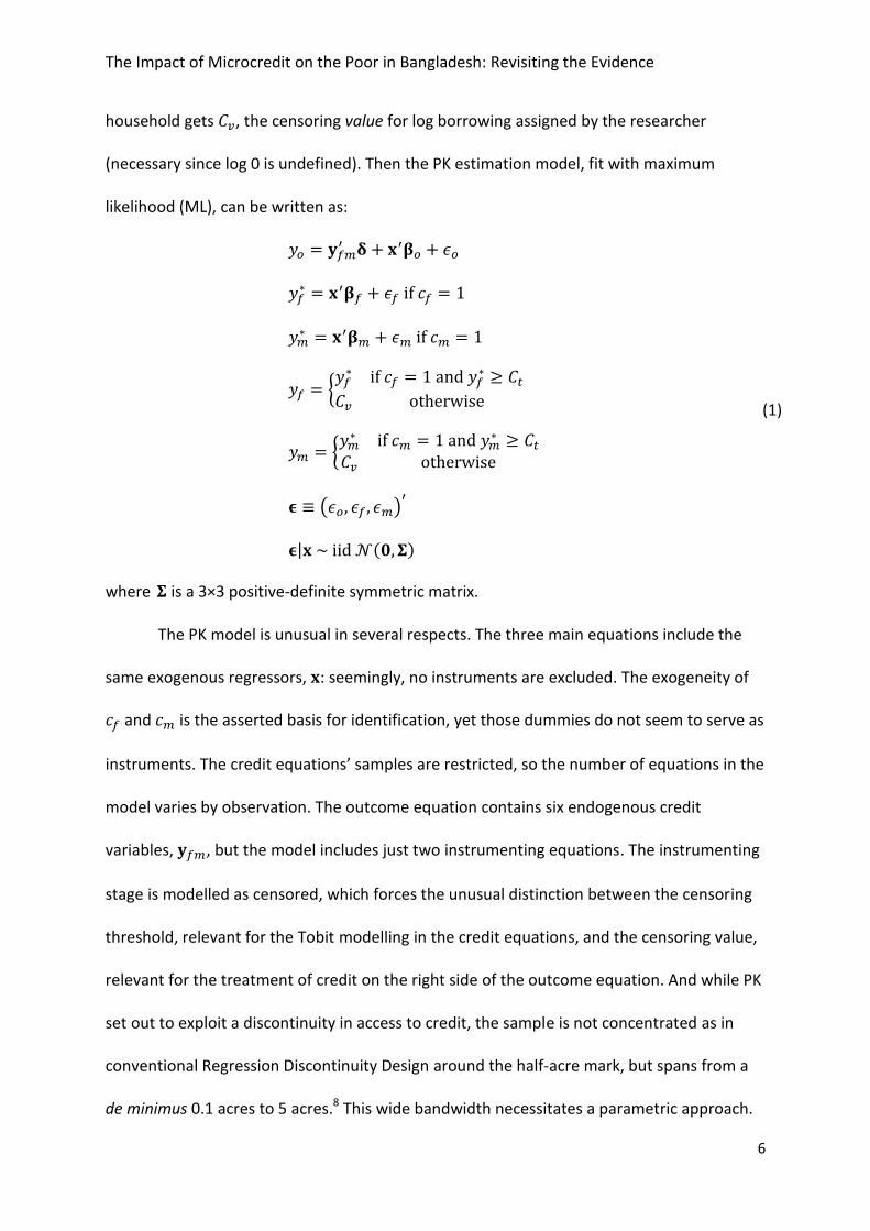
household gets , the censoring value for log borrowing assigned by the researcher

(necessary since log 0 is undefined). Then the PK estimation model, fit with maximum

likelihood (ML), can be written as:

(1)

where is a 3×3 positive-definite symmetric matrix.

The PK model is unusual in several respects. The three main equations include the

same exogenous regressors, : seemingly, no instruments are excluded. The exogeneity of

and is the asserted basis for identification, yet those dummies do not seem to serve as

instruments. The credit equations’ samples are restricted, so the number of equations in the

model varies by observation. The outcome equation contains six endogenous credit

variables, , but the model includes just two instrumenting equations. The instrumenting

stage is modelled as censored, which forces the unusual distinction between the censoring

threshold, relevant for the Tobit modelling in the credit equations, and the censoring value,

relevant for the treatment of credit on the right side of the outcome equation. And while PK

set out to exploit a discontinuity in access to credit, the sample is not concentrated as in

conventional Regression Discontinuity Design around the half-acre mark, but spans from a

de minimus 0.1 acres to 5 acres.8 This wide bandwidth necessitates a parametric approach.


7

1.3 A closer look at assumptions A key to understanding some of these unusual characteristics is to note that the last line of

(1) elides a complexity. The and equations are not defined over the full sample, so ,

, and the joint distribution are not either. So to state the distributional

assumption precisely, we distinguish the four possible cases of credit availability by gender.

We use combinations of , , and subscripts to denote subvectors of and submatrices

of corresponding to combinations of the equations for the outcome, female credit, and

male credit. A precise statement of the distributional assumption (not spelled out in PK) is

then:

where and . Every case implies . Thus

(2)

That is, knowing credit availability by gender tells us nothing about the distribution of .

This is how the identification strategy implies and requires that credit choice is exogenous.

One can gain further intuition by innocuously inserting and into the latent

credit equations in (1):

(3)

This communicates the idea that and are the instruments, being excluded from the

equation. And since includes a constant, and are now seen as instruments too.

One important question about the PK estimation model is whether its distributional


8

assumptions must hold strictly for the estimates of to be consistent. ML estimation of

misspecified models can be consistent for some parameters (White, 1982). For example,

linear LIML is naturally derived from a model that assumes iid normal errors, but is

consistent under substantial violations of that assumption: errors need not be normal, and

they need only be uncorrelated with the instruments, not independent (Anderson and Rubin

1950).9

The nonlinearities in the PK estimator turn out to make it less robust to such

violations. For example, the estimator is inconsistent if has skewness, as simulations in

the appendix demonstrate. Similarly, if the first-stage Tobit models are not exactly correct,

then the estimator should be presumed inconsistent (Angrist and Krueger 2001). In contrast,

a linear instrumental variables (IV) estimator defined along the lines of (3)—instrumenting

with and and dispensing with the Tobit modelling of borrowing—is consistent

regardless of the true functional form and error distribution of the first stage (Kelejian,

1971).

The PK specifications that include village dummies in , among them the headline

regression suggesting that microcredit reduces poverty, are akin to the difference-in-

differences (DID) estimator with controls. The two dimensions of difference are the

eligibility of a household for microcredit (indicated by ) and the availability of microcredit

in a village ( and ). As in DID, identification comes from variation associated with the

excluded products and conditional on the included factors , , and ( and

being controlled for through the village dummies).10 The validity of the exclusion

assumption is open to question (Morduch, 1998). For example, in villages where eligible

households are relatively well-off, credit group formation may be more likely. In this way,

village effects may interact with eligibility to cause outcomes through channels separate


9

from microcredit.

2. Replication Pitt (2011) provides a data set adequate for replicating the PK regression of primary interest,

with as log per-capita household consumption. The first and second moments of

regression variables in the Pitt (2011) data closely match those reported in PK—though not

exactly.11 (See Table 1 and Table 2.)

The five other PK outcomes are not in the Pitt (2011) data, nor in a set sent earlier to

us by Mark Pitt. So we construct those outcomes from the underlying survey data. Among

the five, the match is extremely good for male labour supply and boys’ and girls’ school

enrolment. It is poorer for female labour supply. But here we have reason to doubt PK’s

aggregates. PK (2002, Table 1) reports the same means alongside mathematically

incompatible seasonal subaverages. Finally, the biggest discrepancies are in female-owned

non-land assets. As shown, we obtain a much better match if we include land in ‘nonland’

assets.

The first column of Table 3 shows PK’s preferred fixed-effect estimates of the impact

of microcredit on household consumption by gender and lender. The second shows our best

replication, using the cmp program for Stata (Roodman, 2011).12 The matches for the female

credit coefficients are excellent. Those for male credit are statistically similar. The estimated

correlations of with and , labelled ‘ female’ and ‘ male,’ also match well.13 The

apparent small differences in the underlying data, as well as subtle differences among

nonlinear estimation packages (McCullough and Vinod 2003), probably explain the

imperfections in the match.

Near the bottom of Table 3 are reported the skew and kurtosis of the estimation


10

residuals. In every case they differ from the values for the normal distribution (skew of 0

and kurtosis of 3) with significance levels below 10–10 according to the test of D’Agostino,

Belanger, and D’Agostino Jr. (1990).14 We will return later to this violation of the PK model.

3. Specification problems in PK Morduch (1998) identifies several concerns with the headline PK specification. Our analysis

exposes more. This section inventories the problems and applies fixes where possible.

3.1 The logarithm of zero Analysis using the logarithm of credit requires imputing some value for observations where

credit is 0. Here, the choice is doubly tricky. As displayed in (1), the PK estimation model

creates a distinction between the censoring threshold for credit, , and censoring value, .

PK set since 1,000 taka is the smallest observed amount of cumulative total

borrowing. That is, the Tobit likelihoods for the first-stage equations is computed as if every

non-borrowing household had to borrow at least 1,000 taka. But PK set .

That is, in the second-stage equation non-borrowers are modelled as receiving 1 taka of

treatment. Since household consumption is also taken in logs—so that coefficients on credit

are elasticities—the latter assumption implies that, ceteris paribus, moving from non-

borrowing status, proxied by 1 taka, to minimal borrowing status—1,000 taka, or about

$25—has the same proportional impact as moving from 1,000 to 1,000,000 taka of

borrowing. (The highest observed cumulative borrowing is 58,800 taka.) That is a strong,

unstated, and unexamined assumption.

It is also econometrically influential. PK could have set log 10 or log 0.1. The

differences among these choices are pennies in levels, but substantial in logs. The lower the

censoring value, the greater the variance in log credit, thus the smaller the expected best-fit


11

slope coefficients in a regression of consumption on log credit. Figure 1 illustrates by

showing the data with the censoring value at log 1, which PK use, and alternatively at log

1,000. One can see why the slope of a best-fit line would vary substantially as the censoring

value changes. Since the impact estimates in PK are based on this arbitrary choice, their

magnitude is unidentified.15

The deep problem is that the elasticity construct implied by regressing logs on logs

does not allow for zero values. Thus a hypothetical move from non-borrowing to borrowing

status lies outside the construct, and can only be linked to it through an auxiliary

assumption about the impact of such a non-marginal move relative to a marginal increase in

borrowing. A better solution to this conundrum would be to enter borrowing dummies and

borrowing amounts separately in the equation. But we see no good instruments for

borrowing amounts as distinct from borrowing decisions.

In fact, the key instruments in the PK model, and , can be expected to be strong

only for the borrowing decision. Thus to the extent that the PK estimator is succeeding in

identifying impacts, these are mainly the average impacts of becoming a borrower. In this

light, the PK conclusion about the marginal impacts of borrowing arises from a conversion of

an average impact into a marginal one by way of an assumption that becoming a minimal

borrower has the same proportional impact as increasing borrowings a thousandfold.

More practical than simultaneously modelling the borrowing decision and borrowing

amount is to focus on the first: simply model borrowing as dichotomous. This circumvents

the question of how to handle the log of 0 while focusing on the variation in borrowing for

which credit choice is a potentially strong instrument. Ironically, PK’s use of an implausibly

low censoring value pushes their model in this more meaningful direction by causing the

variation associated with the borrowing decision—the wide gap between log 1 and log


12

1,000 in Figure 1—to dominate total variation in credit. So it is not surprising that

‘probitizing’ the credit model in this way corroborates PK’s results. (See column 3 of Table

3.) Going by these new point estimates, households in which women took microcredit had

about per cent higher per-capita consumption. However, PK’s translation

of this average effect into a marginal one—‘household consumption expenditure increases

18 taka for every 100 additional taka borrowed by women…compared with 11 taka for

men’—appears unfounded.

3.2 A missing discontinuity PK buttress the claim that and are exogenous by pointing to two factors: the

arbitrariness of the half-acre eligibility cut-off, and the exogeneity of landownership. On the

latter, they write, ‘Market turnover of land is well known to be low in South Asia. The

absence of an active land market is the rationale given for the treatment of landownership

as an exogenous regressor in almost all the empirical work on household behaviour in South

Asia’ (p. 970). However, this appears to be a case for landholdings being external to the

model (Heckman, 2000). Exogeneity is a distinct notion (Brock and Durlauf, 2001; Deaton,

2010), requiring that the characteristic of owning more than half an acre relates to

outcomes only through microcredit (after linearly conditioning on controls, including log

landholdings).

Thus whether an eligibility dummy based on the half-acre rule is exogenous is a

distinct question from whether land turnover was low in the study area. The question is also

less relevant than first appears, for PK use no such dummy (Morduch, 1998). PK’s eligibility

dummy is defined strictly on the half-acre rule only for villages without microcredit. In

program villages, 203 of the 905 borrowing households—a weighted 24 per cent of


13

borrowing households—owned more than half an acre before borrowing. PK classify all as

eligible. As a result, the dummy departs substantially from the de jure definition of

eligibility.

So there are two caveats for the estimation here: the identifying variation in lacks

discontinuity, and it is presumably endogenous. To illuminate the matter, we follow the

advice of Imbens and Lemieux (2008) on preliminaries to discontinuity-based regression, by

plotting the key regressors and against the continuous forcing variable, household

landholdings before borrowing. See Figure 2. We perform Lowess regressions separately for

the below- and above-threshold subsamples in order to allow a discontinuity at the half-

acre mark.16 95-per-cent confidence intervals are shown. The plots are restricted to

households for which (for female borrowings) or (male borrowings). Per PK,

non-borrowers are assigned 1 taka of borrowing. Effective enforcement of the half-acre

eligibility criterion would cause the borrowing curves to plunge near the threshold. Instead

they hop a bit in opposite directions, without statistical significance. Evidently, loan officers

were either unaware of the formal half-acre eligibility rule or pragmatically bending it to

extend credit to borrowers who seemed reliable and who were, after all, poor by global

standards. Some over-half-acre households that borrowed may have met an alternative

eligibility criterion (see footnote 5), but this cannot explain such substantial mistargeting. At

any rate, the asserted basis for quasi-experimental identification is invisible in the data.

Morduch (1998) makes most of these points. Pitt’s (1999) argues that the true

microcredit eligibility rule is ‘unknown’ (presumably being a function of land quality, not just

quantity, and other factors tied to poverty) and that identification in PK’s IV set-up requires

only that the exogenous half-acre rule drive a component of variation in borrowing. In effect,

Pitt casts the identification strategy as a Fuzzy Regression Discontinuity design.17


14

This argument has two weaknesses. First, it concedes that the claimed quasi-

experiment, central to PK’s bid for credibility, is only asserted, not observed. Second, even if

the quasi-experiment did occur, the PK model does not exploit it. In light of the pervasive

non-enforcement of the rule evident in Figure 2, the eligibility dummy as defined and used

by PK, and thus the key instruments, and , is not defined by this rule and

should be presumed endogenous. To properly exploit the quasi-experiment, PK’s de facto

eligibility dummy should be replaced by a de jure one built strictly on the half-acre rule.

We check the PK regression for robustness to this change. How requires explanation.

A naïve implementation would replace throughout the model with

and redefine the credit choice dummies as and . A

problem with this approach is that the mistargeted households that borrowed would now

be excluded from the first-stage equations since for them and and

define the first-stage samples. To include them in the instrumenting equations while

defining the samples for those equations in a way that is more plausibly exogenous, we

expand their samples to all households in villages with credit programs of the given gender.

This puts all households in program villages, regardless of eligibility however defined, in the

‘treatment’ group. As Pitt (1999) points out, erring on the side of modelling more

households as having access to credit does not affect consistency. Within these expanded

samples, credit can then be instrumented as in (3) with and .

Roughly speaking, this instruments all treatments, targeted and mistargeted, with intent to

treat.

Column 4 of Table 3 reports the results of such an alteration. It strengthens the PK

results for female microcredit. This does not mean the PK instruments are valid (the lack of

a discontinuity poses a serious problem for the motivation behind PK’s identification


15

strategy). But it does suggest that one potential source of invalidity, endogeneity tied to

violation of the eligibility rule, is not driving the PK results.

3.3 Correlation between the instruments and error We next examine more directly whether the instruments are valid even after the de jure

redefinition. We do this by adding them linearly to the second-stage equation. The PK

estimates are still technically identified under this change because their model’s first stage is

nonlinear. The second half of Table 3 reports the results of such tests. The first column

shows the effect of introducing just and into the second stage while using PK’s de

facto eligibility definition. The next column adds all of and . The second pair of

columns parallels the first, but using the de jure definition. In all cases, the newly included

instruments have clear explanatory power. As shown near the bottom of the table, the p

values on the Wald F tests for the joint significance of the included instruments are less than

0.05.18

Yet the PK results persist. Since including the instruments linearly does not drive out

the PK results, it appears that nonlinear relationships between credit and household

spending are generating the identification in PK. These relationships could be based on

exogenous variation, but the linear endogeneity of the instruments makes this seem less

likely.

3.4 Instability We discovered that the PK likelihood on the PK data has two local maxima. (First two

columns of Table 4.) The local maximum with the higher log likelihood yields the positive

results in PK. The second one, not reported in PK, puts mildly negative coefficients on

female credit and reverses the sign on the estimated the correlation between and (‘


16

female’). Its lower log likelihood, –6,548 instead of –6,541, arguably favours the published

mode. But how meaningful this comparison is is not clear since the likelihood model is

incorrect. As noted in section 2, the error is not normally distributed.

To illustrate the situation, we graph the likelihood as a function of ,

where and are the two modes and ranges between –1 and +2. While all 255

parameters vary in this cross-section of the likelihood, the coefficients that change most are

on female microcredit. So we label the axis with the coefficient on female borrowings

from the Grameen Bank. (See Figure 3.)19

The bimodal likelihood appears to lead to a bimodal estimator. The mechanism is

intuitive: small changes in the data can perturb the relative heights of the two peaks or raise

the trough between them just enough to turn two peaks into one. To demonstrate, we

bootstrap the estimator’s distribution with 1,000 samples from the PK data, drawing with

replacement. Since PK reweight observations within villages, we draw at the village level

(Field and Welsh, 2007). For each sample, we maximize the likelihood twice, starting the

searches at the estimates in columns 1 and 2 of Table 4. When two modes are found, the

higher is retained. Figure 4 shows the distribution of this estimator as a histogram and as an

Epanechnikov kernel density plot. 37 per cent of the distribution is below zero. Going by this

bootstrapped distribution, which is more reliable under the circumstances than the classical

standard errors, we cannot reject the null of zero or negative impact of female borrowing at

conventional significance levels. The previously unremarked instability helps explain why the

specification discrepancies in the first edition of this paper flipped the coefficients on female

microcredit.

The theory of Maximum Likelihood does not guarantee that a correct likelihood is

asymptotically unimodal. However, it does assure that when there are multiple modes, an


17

estimator that picks the highest one will converge to the true parameters. The estimator will

still be asymptotically unimodal. The apparent bimodality of the PK estimator, as distinct

from the likelihood, is therefore a first-order concern. What is causing it? Our investigations

suggest two factors: the model-violating skew in the second-stage error; and instrument

weakness, at least in a subsample, brought on by the splitting of the borrowing variables by

gender. Reducing either problem alone eliminates the bimodality—and the PK finding of

positive impact—which suggests that the two factors are interacting to produce the

published results. Meanwhile, a linear IV estimator whose required assumptions are more

compatible with the data produces impact estimates indistinguishable from zero.

One way to remove the bimodality in the likelihood is to drop the observations in the

long right tail in household consumption, the ones most responsible for the model-violating

skew in the error. To demonstrate, we estimate our replication regression 50 times, first for

the full sample, then excluding the highest-consumption observation, then the highest two,

etc., up to the highest 49, initiating the searches in the same way as for Figure 4. Figure 5

plots the discovered modes along with conventionally computed 95 per cent confidence

intervals, once more labelling with the female Grameen impact coefficient. The upper-

rightmost dot represents our replication of the full-sample headline PK specification. The

lower-rightmost dot is the alternate mode documented in Table 4. Scanning from right to

left, we see that the two modes collapse into one near zero after dropping the 16 highest-

consumption observations, which are associated with 14 households and constitute 0.4 per

cent of the sample on a weighted basis.20

Another change that eliminates the finding of positive impact involves revisiting the

gender split in the model. Recall that PK’s key instruments and are products of two

factors: the eligibility status of households, , and the presence in a village of credit groups


18

of each gender, and . PK defend the exogeneity of the first factor, but not the second.

Nor seemingly, is the latter as crucial to their project: since the main goal is to estimate the

overall impact of microcredit, it is not obviously necessary for PK to disaggregate the model

by gender. If they did not, they could define a single program placement dummy ; a single

credit availability dummy ; and a single instrumenting equation for household

borrowings. Because the exogeneity of and is neither essential nor defended, we try

dispensing with it, by aggregating credit across gender. (See Table 4, column 3.) As one

might expect, the point estimates of impact lie approximately halfway between those the

replication puts on male and female credit. But statistical significance is lost, and we no

longer find a second mode.

The loss of significance may merely be a sign of an imperfect model: female and

male credit may have different impacts and so are better disaggregated. But the next four

specifications challenge this position. Here, we retain PK’s split by gender and instead drop

parts of the sample. Since the sections dropped are defined by and , asserted

exogenous, this step does not introduce bias under PK’s assumptions. First we drop

households in villages where men can borrow. The resulting comparison of female-only to

no-credit villages generates another estimate of the impact of microcredit for women. The

next regression does the same for men. The third excludes only villages where both women

and men can borrow. All these variants destroy the PK results.21

In contrast, the last variant (in the last column) is restricted to the complement of

the previous one, villages in which both women and men could borrow. The coefficients on

female credit are almost the same as in PK. Yet it is here that the instrumentation is weakest

since here, and . So the gender-differentiated choice instruments

cannot differentiate impacts by gender. The PK result is strongest where the instruments


19

are weakest.

Other arguments also point to instrument weakness as a source of the instability. In

2SLS and linear LIML, weak instrumentation is known to exaggerate the tendency toward

bimodality (Phillips, 2006). Simulations in PK (2012) show how the same can happen in the

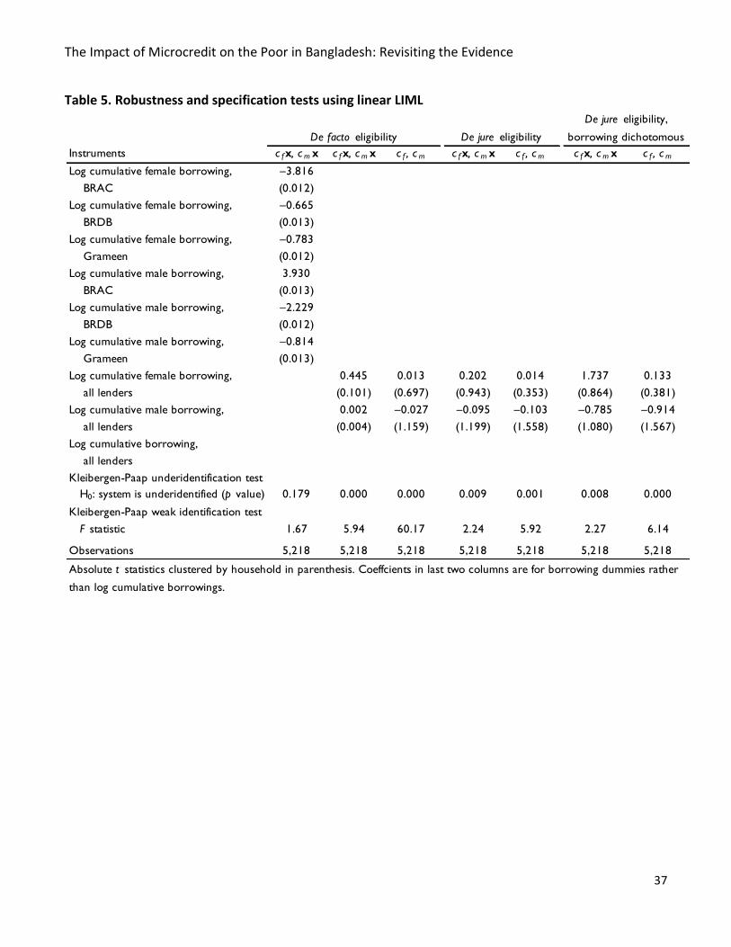
nonlinear PK estimator.22 For a final probe into this matter, we run linear LIML, which opens

the door to established tests of weakness. Linear LIML also has the advantage of being

robust to deviations from normality, so it provides an additional check on the PK results. In

particular, we expand the credit equations to the full sample, model credit as linear, and

instrument with and .23 In our first run, with six instrumented credit variables, it is

not even certain that the regression is identified; we can reject the null of

underidentification only at (column 1 of Table 5). Combining credit variables

across lenders reduces the burden on the instruments and lifts the regression past that test

(column 2), but the Kleibergen-Paap (2006) F statistic of weakness, is 5.944. This is well

below Staiger and Stock’s (1997) rule-of-thumb minimum of 10 for 2SLS. On the other hand,

the test here may be distorted by the high number of instruments. When we strip the

instrument set down to and (column 3), the weak identification check greatly

improves: across the full sample at least, identification is strong.

The linear regressions require for consistency that and be uncorrelated with

the error, an assumption questioned in section 3.3. In order to reduce endogeneity, we

replace the de facto eligibility definition with the de jure as before. The change produces

essentially the same pattern of results, albeit with weaker instruments (columns 4 and 5 of

Table 5). Given the apparently endogenous recoding of the de facto eligibility variables, it is

unsurprising that they are stronger, if more suspect, instruments for borrowing. For

completeness, we repeat the previous two regressions while modelling credit as binary, for


20

reasons given in section 3.1 (last two columns of Table 5). The last of these regressions is

our preferred specification, being the most conservative and robust in PK and the present

paper.

We draw two observations from the linear regressions. One is that these robust

estimators never produce impact coefficients distinguishable from 0: in our experience,

obtaining the PK result requires an estimator whose assumptions are especially

incompatible with the data. Second, however, is that de facto credit choice instruments that

PK use actually do not appear weak in the most conservative gender-split regression

(column 3 of Table 5).24 Our best synthesis of the evidence relating to instrument weakness

is that the PK results are generated in part by instrument weakness in a subsample, as

suggest by the last regression of Table 4. This notion has little meaning or relevance for

linear estimators, but appears more relevant for nonlinear ones. What is not in doubt is that

we can only produce the PK result with an estimator whose assumptions conflict with the

data, and that reducing that conflict—dropping the 16 most extreme consumption

outliers—eliminates the PK result even when using the PK estimator.

4. Other outcomes We attempt to replicate PK’s results for the five outcomes other than per-capita household

consumption. (See Table 6.) None of the results match PK exactly, but all are similar in signs

and significance. The worst match, as in Table 2, is for female non-land assets; although

even here, the results are not statistically different. Adding land to nonland assets gave us

reasonable matches in first and second moments in Table 2, but it does not aid us in

matching regression results. We check all regressions for a second mode in the same

manner as before. We find one only for male labour supply. The two discovered modes


21

clash on the sign of the impact of male microcredit borrowing.

Given our doubts about the instrumentation strategy, we think the most important

thing to observe about the six PK LIML fixed-effects estimates is that they are of two sorts.

Those for female non-land assets, female labour supply, and girls’ and boys’ school

enrolment feature insignificant coefficients on credit, insignificant parameters, and no

apparent bimodality. In contrast, the household consumption and male labour supply

results feature strong impact coefficients, significant parameters, and bimodality that

produces starkly contradictory impact coefficients for one sex. This is further evidence that

bimodality is the proximate cause of the significant results in PK’s household consumption

regression. Notably, this instability arises with the two least-bounded outcomes, the ones

with the most scope for deviation from normality. Log household consumption is an

unbounded variable. Male labour supply is bounded from below but assumes its bounding

value of 0 in only 8.6 per cent of cases on a weighted basis.

5. Conclusion Pitt and Khandker (1998) reinforced some broad ideas about microcredit: that it reduces

poverty, and that it does so especially when given to women. In our view, nothing in the

present paper contradicts those ideas. We stress that absence of evidence—lack of

identification—is not evidence of absence. But the present paper should reduce confidence

in the poverty-reducing power of microcredit to the extent that it rested on PK. Our critical

conclusions about PK, combined with the muted results of the randomized trials of

microcredit, mean that 35 years into the microfinance movement, credible evidence in

favour of the proposition that microcredit reduces poverty is scarce (Armendáriz and

Morduch, 2010, chapter 9; Odell, 2010; Duvendack et al., 2011; Roodman, 2012a, chapter 6).


22

Our work replicating Pitt and Khandker (1998) has left us with great admiration for

its sophistication and creativity. But its econometric sophistication obscures problems:

an imputation for the log of the treatment variable when it is zero that is

undocumented, influential, and arbitrary at the margin, making the impact size

essentially identified;

the absence of a discontinuity that is asserted as central to the identification

strategy;

a reclassification of formally ineligible but borrowing households as eligible, which

presumably introduces endogeneity into the asserted quasi-experiment;

a linear relationship between the instruments and the error;

disappearance of the results when villages where both genders could borrow are

excluded;

instability in the estimator;

disappearance of the results after dropping 16 outliers, 0.4 per cent of the sample,

that especially violate a modelling assumption.

Our analysis raises a broad question about the value of non-randomized studies. Our

prior is that exclusive reliance on one type of study, such as randomized ones, is not optimal.

But for non-randomized studies to contribute to the measurement of causation in social

systems, the quality of the natural experiments must be high, and demonstrated.25

Our replication also raises questions about quality control in the production of

economics. Although some of the econometric tools we bring to bear were not developed

or were less practical in the late 1990s than now, many relevant specification checks were

practical: for the presence of an asserted discontinuity, for the normality of the errors, for

robustness to outlier removal, for robustness to aggregation by gender; and for robustness


23

to switching to linear LIML. Of course, hindsight is 20/20. So we point up this issue not to

engage in retrospective perfectionism but to draw lessons for social science today. What

was and is reasonable to expect is that authors, reviewers, and journal editors take steps to

prevent methodological complexity from obscuring fundamental issues of identification.

Assumptions should be checked to the extent they can be. Dependence on secondary

assumptions, such as that required in PK for the identification of impacts by gender, should

be tested. Where possible, complex estimators should be checked by simpler ones.

A more radical strategy for quality control is transparency: sharing data and code

starting at the working paper stage. Freely circulating data and code facilitates the scrutiny

needed for science to proceed. The stakes are particularly high for research that influences

policy (McCullough and McKitrick 2009). The Journal of Political Economy, which published

PK, now requires such disclosure, although its data archive is among the least accessible

(McCullough, McGeary, and Harrison, 2008). Our own transparency allowed Pitt (2011) to

find the errors in our initial attempts at replication, which in turn led us to the most serious

problems documented here.26 Had JPE enforced open data and code sharing in 1998, the

debate over this study might have been resolved long ago.

Notes 1 Randomized studies have found that access to capital increases average profitability of

male-run microenterprises, but challenged the central claim that it does so for female-run

businesses (see McKenzie and Woodruff 2008 on male-run businesses in Mexico and de Mel,

McKenzie, and Woodruff 2008 on male- and female-run businesses in Sri Lanka). Other

randomized studies find no support for the claim that microcredit increases household

consumption within a few years (Banerjee et al., 2013; Karlan and Zinman 2011; Crépon et


24

al., 2011; Attanasio et al., 2011; Augsburg et al., 2012; Angelucci, Karlan, and Zinman, 2013).

2 For example, Appelbaum (2008), Yunus (1999; 2007; 2008), Yunus and Abed (2004). The

5% figure comes from Khandker (1998: 56), which extrapolates from PK.

3 McCullough and Vinod (2003, p. 888) advocate for replication emphatically. In their view,

“Replication is the cornerstone of science. Research that cannot be replicated is not science,

and cannot be trusted either as part of the profession’s accumulated body of knowledge or

as a basis for policy. Authors may think they have written perfect code for their bug-free

software package and correctly transcribed each data point, but readers cannot safely

assume that these error-prone activities have been executed flawlessly until the authors’

efforts have been independently verified. A researcher who does not openly allow

independent verification of his results puts those results in the same class as the results of a

researcher who does share his data and code but whose results cannot be replicated: the

class of results that cannot be verified, i.e., the class of results that cannot be trusted.”

4 A compounding problem is journals’ relative lack of interest in publishing replication and

re-analysis, in favour of publishing new findings. For a sustained perspective on the

problems posed for the advancement of social science, see McCullough and Vinod (2003),

McCullough et al. (2008), and McCullough and McKitrick (2009).

5 Among the three creditors, at least Grameen also officially applied an alternative eligibility

criterion: ownership of assets worth less than one acre of medium-quality land (The

Grameen Bank Ordinance, as amended through 2008, §2(h).) However, PK rely exclusively

on the half-acre rule in their analysis.

6 PK measure credit as the simple sum of borrowings since 1986. If a woman borrowed

1,000 Bangladeshi taka, repaid it over a year, then repeated with cycles of 2,000, 3,000,


25

4,000, and 5,000, that would count as 15,000 in borrowings.

7 PK include specifications that control for a set of village characteristics instead of a full set

of village dummies. But the fixed-effect specifications are preferred, so we focus exclusively

on them. Morduch (1999) notes that the village-level fixed effects are designed to control

for non-random program placement, but in this instance they will only do so under

restrictive assumptions. Even with village-level fixed effects, bias can emerge when

programs base their placement decisions on the characteristics of sub-village groups. For

example, programs may favour villages where part of the village is prospering and another

segment is, so far, excluded from the gains. The village-level fixed effects will only control

for the average characteristics of the village sample.

8 PK exclude 41 households owning more than 5 acres.

9 Lack of correlation, recall, is lack of linear relationship. As an example, a variate

symmetrically distributed around 0 is uncorrelated with its square but entirely related to it.

10 The comparison to standard DID is not exact because includes additional controls, and

and contain additional instruments.

11 In addition, the Pitt (2011) data set, like PK, has the disadvantage of treating current

students as having zero years of schooling.

12 Pitt (2011) first replicated PK with cmp. Our replication differs only in using first-round

data for all three survey rounds in the first-stage equations, which, according to Pitt (2011),

is what PK did.

13 The first edition of this paper failed to replicate. Pitt (2011) pointed out two key

discrepancies in our specification. We needed to include as a control, and we needed to

censor ‘log 0’ credit observations with log 1,000 rather than log 1. The first of these choices


26

is documented in PK, the second not. Roodman and Morduch (2011) provide details.

14 In an earlier version of this paper, we neglected to incorporate sampling weights into

these calculations (PK, 2012). We correct the error here, and it increases the apparent

deviations from normality.

15 In fact, setting flips the sign of the impact of female borrowing. This helps

explain why the first edition of this paper failed to match PK, and is a sign of the instability

discussed in section 3.4.

16 Taking Stata’s defaults, the bandwidth for the Lowess regressions is an (unweighted) 80%

of the sample. The local weighting function is tricubic and incorporates PK’s sample weights.

17 PK footnote 16: ‘The quasi-experimental identification strategy used here is an example of

the regression discontinuity design.’

18 The first edition of this paper tested instrument validity through overidentification tests

on analogous 2SLS regressions, and reached the same conclusion. The new approach is an

improvement because it is rooted in PK’s specification.

19 The picture is nearly identical for all three lenders.

20 Since the concern about normality pertains to the residuals in the regression, not the

outcome variable, it is arguably more correct to perform this exercise with respect to the

former. On the other hand, if the regression is wrong, then so are the residuals computed

from it. At any rate, using the residuals produces a similar graph, in which the two modes

collapse more slowly.

21 No estimate for BRAC microcredit is available in the regression excluding villages where

women could borrow because BRAC did not lend to men.

22 In an effort to rebut the arguments made here, they try to show that bimodality in the


27

likelihood is a normal feature of the PK estimator. However, their simulations produce

bimodality only by deviating from the PK model and estimator in two major ways that

weaken instruments. They simulate borrowings as averaging zero in the treatment group, so

that average treatment is the same for borrowers and non-borrowers and credit choice is a

perfectly weak instrument for treatment. And they control for credit choice rather than

instrumenting with it. (The other components of and remain as instruments.) As a

result, the simulations bolster rather than rebut the hypothesis of a link between

instrument weakness and bimodality.

23 After proposing this approach (PK, 1998, note 16) and relying on it (Pitt, 1999), PK (2012)

challenge it. They argue that even when identification is valid and strong in the PK estimator,

the instruments in the corresponding linear IV estimator are weak. However, simulations in

our appendix and in Pitt (1999) demonstrate the efficacy of linear IV. And the PK (2012)

theoretical argument confuses individual and collective weakness (Roodman, 2012b). If is

a weak instrument for and is weak for , and can still be collectively strong for

and .

24 PK (2012) challenge these regressions as presented in the working paper version. But our

discussion here notes, as before, that the first regression in Table 5 is underidentified, and

we do not rely on it for inference. And we here add the exactly identified regressions, which

eliminate PK’s concern about instrument proliferation and the rank-deficient covariance

matrix of the moments.

25 For more, see, for example, the debate between Banerjee and Duflo (2009) and Deaton

(2010).

26 Data and code for this paper are at j.mp/gpXmI1.

http://j.mp/gpXmI1


28

References Anderson, T.W. and Rubin, H. (1950) The asymptotic properties of estimates of the parameters of a

single equation in a complete system of stochastic equations. Annals of Mathematical Statistics,

21(4), pp. 570–582.

Appelbaum, R. (2008) The man who is creating a world without poverty. Santa Barbara Independent.

January 10.

Angelucci, M., Karlan, D. and Zinman, J. (2013) Win some lose some? Evidence from a randomized

microcredit program placement experiment by Compartamos Banco.

Angrist, J. D. and Krueger, A.B. (2001) Instrumental variables and the search for identification: From

supply and demand to natural experiments. Journal of Economic Perspectives, 15(4), pp. 69–85.

Armendáriz de Aghion, B. and Morduch, J. (2010) The Economics of Microfinance. 2nd ed. Cambridge,

MA: The MIT Press.

Attanasio, O., Augsburg, B., De Haas, R., Fitzsimons, E. and Harmgart, H. (2011) Group lending or

individual lending? Evidence from a randomised field experiment in Mongolia. Working Paper

11/20. Institute for Fiscal Studies.

Augsburg, B., De Haas, R., Harmgart, H. and Meghir, C. (2012) ‘Microfinance at the margin:

Experimental evidence from Bosnia and Herzegovina.’ European Bank for Reconstruction and

Development.

Banjerjee, A.V. and Duflo, E. (2009) The experimental approach to development economics. Annual

Review of Economics 1:151–178

Banerjee, A.V., Duflo, E., Glennerster, R. and Kinnan, C. (2013) The miracle of microfinance? Evidence

from a randomised evaluation. Working Paper 18950. NBER.


29

Baum, C., Schaffer, M.E. and Stillman, S. (2007) Enhanced routines for instrumental variables/GMM

estimation and testing. Stata Journal, 7(4), pp. 465–506.

Brock, W.A. and Durlauf, S.N. (2001) Growth empirics and reality. World Bank Economic Review, 15(2),

pp. 229–271.

Chemin, M. (2008) The benefits and costs of microfinance: Evidence from Bangladesh. Journal of

Development Studies, 44(4), pp. 463–484.

Crépon, B., Devoto, F., Duflo, E. and Parienté, W. (2011) Impact of microcredit in rural areas of

Morocco: Evidence from a randomized evaluation. Massachusetts Institute of Technology.

D’Agostino, R. B., Belanger A. J. and D’Agostino Jr., R. B. (1990) A suggestion for using powerful and

informative tests of normality. American Statistician, 44, pp. 316–321.

Deaton, A. (2010) Instruments, randomization, and learning about development. Journal of Economic

Literature, 48(2), pp. 424–455.

Duvendack, M. and Palmer-Jones, R. (2012) High noon for microfinance impact evaluations: Re-

investigating the evidence from Bangladesh. Journal of Development Studies, 48(12), pp. 1864–

1880.

Duvendack, M., Palmer-Jones, R., Copestake, J.G.. Hooper, L., Loke, Y. and Rao, N. (2011) What Is the

Evidence of the Impact of Microfinance on the Well-Being of Poor People? EPPI-Centre, Social

Science Research Unit, Institute of Education, University of London.

Field, C.A. and Welsh, A.H. (2007) Bootstrapping clustered data. Journal of the Royal Statistical Society

B, 69(3), pp. 369–390.

Heckman, J.J. (2000) Causal parameters and policy analysis in economics: A twentieth century

retrospective. Quarterly Journal of Economics, 115(1), pp. 45–97.


30

Karlan, D. and Zinman, J. (2011) Microcredit in theory and practice: Using randomized credit scoring for

impact evaluation. Science, 332(6035), pp. 1278–1284.

Kelejian, H.H. (1971) Two-stage least squares and econometric systems linear in parameters but

nonlinear in the endogenous variables. Journal of the American Statistical Association, 66(334), pp.

373–374.

Kleibergen, F. and Paap, R. (2006) Generalized reduced rank tests using the singular value

decomposition. Journal of Econometrics, 127(1), pp. 97–126.

McCullough, B.D., McGeary, A. and Harrison, T.D. (2008) Do economics journal archives promote

replicable research? Canadian Journal of Economics, 41(4), pp. 1406–1420.

McCullough, B.D. and McKitrick, R. (2009) Check the numbers: The case for due diligence in policy

formation. Fraser Institute.

McCullough, B.D. and Vinod, H.D. (2003) Verifying the solution from a nonlinear solver: A case study.

American Economic Review, 93(3), pp. 873–892.

De Mel, S., McKenzie, D. and Woodruff, C. (2008) Returns to capital in microenterprises: evidence from

a field experiment. Quarterly Journal of Economics, 123(4), pp. 1329–1372.

McKenzie, D. and Woodruff, C. (2008) Experimental evidence on returns to capital and access to

finance in Mexico. World Bank Economic Review 22 (3), pp. 457–482.

Morduch, J. (1998) Does microfinance really help the poor? New evidence from flagship programs in

Bangladesh. New York University. j.mp/bC3Tge.

Morduch, J. (1999) The microfinance promise. Journal of Economic Literature, 37(4), pp. 1569–1614.

Odell, K. (2010) Measuring the Impact of Microfinance: Taking Another Look. Grameen Foundation.

Phillips, P.C.B. (2006) A remark on bimodality and weak instrumentation in structural equation

http://j.mp/bC3Tge


31

estimation. Paper 1171. Cowles Foundation for Research in Economics. Yale University.

Pitt, M.M. (1999) Reply to Jonathan Morduch’s ‘Does microfinance really help the poor? New evidence

from flagship programs in Bangladesh.’ Brown University. j.mp/dLNltJ.

Pitt, M.M. (2011) Response to Roodman and Morduch’s ‘The impact of microcredit on the poor in

Bangladesh: Revisiting the evidence.’ Brown University. j.mp/j4x2xV.

Pitt, M.M. (2012) Gunfight at the not OK Corral: Reply to ‘High noon for microfinance’. Journal of

Development Studies, 48(12), pp. 1886–1891.

Pitt, M.M. and Khandker, S.R. (1998) The impact of group-based credit on poor households in

Bangladesh: Does the gender of participants matter? Journal of Political Economy, 106(5), pp. 958–

996.

Pitt, M.M. and Khandker, S.R. (2002) Credit programs for the poor and seasonality in rural Bangladesh.

Journal of Development Studies, 39(2), pp. 1–24.

Pitt, M.M. and Khandker, S.R. (2012) Replicating Replication: Due Diligence in Roodman and Morduch’s

Replication of Pitt and Khandker (1998). Working Paper 6273. World Bank.

Roodman, D. (2011) Estimating fully observed recursive mixed-process models with cmp. Stata Journal,

11(2), pp. 159–206.

Roodman, D. (2012a) Due Diligence: An Impertinent Inquiry into Microfinance. Washington, DC: Center

for Global Development.

Roodman, D. (2012b) Perennial Pitt and Khandker. David Roodman’s Microfinance Open Book Blog. 10

December. j.mp/11LrVRI.

Roodman, D. and Morduch, J. (2011) Comment on Pitt’s Responses to Roodman and Morduch (2009).

Center for Global Development.

http://j.mp/dLNltJ

http://j.mp/j4x2xV

http://j.mp/11LrVRI


32

Staiger, D. and Stock, J.H. (1997) Instrumental variables regression with weak instruments.

Econometrica, 65(3), pp. 557–586.

White, H. (1982) Maximum likelihood estimation of misspecified models. Econometrica, 50(1), pp. 1–

25.

Yunus, M. (1999) The Grameen Bank. Scientific American. November.

Yunus, M. (2007) Q&A with Muhammad Yunus. Interview on ‘NOW.’ PBS. j.mp/oEeNni.

Yunus, M. (2008) Credit for the poor. Harvard International Review. January.

Yunus, M. and Abed, F. (2004) Responses to New York Times editorial regarding new US law on poverty

measurement tools. j.mp/o5xjq1.

http://j.mp/o5xjq1


33

Table 1. Weighted means and standard deviations of individual- and household-level right-side variables, first survey round, as reported in PK and in reconstructions


34

Table 2. Weighted means and standard deviations of endogenous variables as reported in PK and in reconstructions

PK New PK New PK New PK New PK New

Cumulative female borrowing, 5,498.85 5,554.04 2,604.45 2,617.61 2,604.45 2,617.61

first survey round (1992 taka) (7,229.35) (7,580.10) (5,682.40) (5,896.01) (5,682.40) (5,896.01)

N = 779 N = 779 N = 326 N = 326 N = 1,105 N = 1,105 N = 1,105 N = 1,105

Cumulative male borrowing 3,691.99 3,757.37 1,729.63 1,748.91 1,729.63 1,748.91

first survey round (1992 taka) (7,081.58) (7,409.36) (5,184.67) (5,390.53) (5,184.67) (5,390.53)

N = 631 N = 631 N = 263 N = 263 N = 894 N = 894 N = 895 N = 894

Per-capita household spending, 77.014 77.014 85.886 85.886 82.959 82.959 89.661 89.661 84.072 84.072

(41.496) (41.496) (64.820) (64.820) (58.309) (58.308) (66.823) (66.825) (59.851) (59.851)

N = 2,696 N = 2,696 N = 1,650 N = 1,650 N = 4,346 N = 4,346 N = 872 N = 872 N = 5,218 N = 5,218

School enrollment of girls 0.535 0.535 0.528 0.527 0.531 0.530 0.552 0.552 0.534 0.534

(0.499) (0.499) (0.500) (0.500) (0.499) (0.499) (0.498) (0.498) (0.499) (0.499)

N = 802 N = 802 N = 434 N = 434 N = 1,236 N = 1,236 N = 225 N = 225 N = 1,461 N = 1,461

School enrollment of boys 0.566 0.566 0.555 0.556 0.558 0.559 0.550 0.553 0.559 0.558

(0.496) (0.496) (0.498) (0.497) (0.497) (0.497) (0.497) (0.498) (0.497) (0.497)

N = 856 N = 856 N = 468 N = 468 N = 1,324 N = 1,324 N = 265 N = 267 N = 1,589 N = 1,591

Women’s labor supply, 40.328 40.389 37.68 32.467 38.905 35.087 43.934 31.269 39.54 34.467

(70.478) (70.558) (71.325) (64.297) (70.934) (66.529) (74.681) (60.214) (71.432) (65.556)

N = 3,420 N = 3,420 N = 2,108 N = 2,108 N = 5,528 N = 5,528 N = 1,074 N = 1,074 N = 6,602 N = 6,602

Men’s labor supply, 202.758 202.749 185.858 185.758 191.310 191.239 180.940 180.528 189.477 189.346

(10.527) (100.820) (104.723) (104.904) (103.678) (103.897) (98.805) (99.405) (102.902) (103.191)

N = 3,534 N = 3,534 N = 2,254 N = 2,254 N = 5,788 N = 5,788 N = 1,126 N = 1,126 N = 6,914 N = 6,914

Female nonland assets, 7,399.23 2,366.09 4,716.42 1,724.55 5,608.03 1,937.76 1,801.84 831.84 4,970.67 1,752.57

first survey round (taka) (293.02) (6,693.24) (19,901.04) (5,033.62) (23,509.09) (5,645.45) (6,287.49) (2,207.09) (21,649.42) (5,245.48)

Female assets, 7,512.51 4,793.83 5,697.37 1,975.24 5,074.08

first survey round (taka)1 (31,572.90) (19,922.00) (24,443.40) (6,428.01) (22,498.90)

N = 899 N = 542 N = 1,441 N = 292 N = 1,733

First three variables are from Pitt (2011). Remainder are reconstructed from PK survey data. 1Aggregates for this variable are displayed to show their similarity to

PK's reported aggregates for non-land assets.

all three survey rounds

(taka/week)

all survey rounds (hours/month,

aged 16–59)

all survey rounds (hours/month,

aged 16–59)

aged 5–17, first survey round

(yes = 1)

aged 5–17, first survey round

(yes = 1)

Program villages

Participants Nonparticipants Total Nonprogram villages All villages


35

Table 3. Replication and robustness tests of PK fixed-effects LIML household consumption regression


36

Table 4. Tests relating to bimodality and gender


37

Table 5. Robustness and specification tests using linear LIML

Instruments c fx, c m x c fx, c m x c f , c m c fx, c m x c f , c m c fx, c m x c f , c m

Log cumulative female borrowing, –3.816

BRAC (0.012)


BRDB (0.013)


Grameen (0.012)

Log cumulative male borrowing, 3.930

BRAC (0.013)

Log cumulative male borrowing, –2.229

BRDB (0.012)

Log cumulative male borrowing, –0.814

Grameen (0.013)

Log cumulative female borrowing, 0.445 0.013 0.202 0.014 1.737 0.133

all lenders (0.101) (0.697) (0.943) (0.353) (0.864) (0.381)

Log cumulative male borrowing, 0.002 –0.027 –0.095 –0.103 –0.785 –0.914

all lenders (0.004) (1.159) (1.199) (1.558) (1.080) (1.567)

Log cumulative borrowing,

all lenders

Kleibergen-Paap underidentification test

H0: system is underidentified (p value) 0.179 0.000 0.000 0.009 0.001 0.008 0.000

Kleibergen-Paap weak identification test

F statistic 1.67 5.94 60.17 2.24 5.92 2.27 6.14

Observations 5,218 5,218 5,218 5,218 5,218 5,218 5,218

De jure eligibility,

borrowing dichotomous

Absolute t statistics clustered by household in parenthesis. Coeffcients in last two columns are for borrowing dummies rather

than log cumulative borrowings.

De jure eligibilityDe facto eligibility


38

Table 6. LIML fixed-effects estimates of impact of microcredit on outcomes other than consumption, PK and new


39

Figure 1. Household borrowing by women vs. household consumption, with censoring levels of log 1 or log 1,000

Nonborrowers, censored with log 1 as in PK

Nonborowers, if censored

with log 1,000 instead

Borrowers

3

4

5

6

7

0 5 10Log cumulative borrowing (1992 taka)

Log weekly householdexpenditure/capita(1992 taka)


40

Figure 2. Cumulative borrowing vs. household landholdings before borrowing, first survey round, in villages with access to credit for given gender

Classified by PK as eligible

1

10

100

1,000

10,000

0.001 0.01 0.1 0.5 1 10 Household landholdings before borrowing (acres)

Men

Classified by PK as eligible

1

10

100

1,000

10,000

Cumulative borrowing (1992 taka)

Women


41

Figure 3. A cross-section of the PK likelihood on PK data, with two local maxima marked

(0.043, -6541)(-0.018, -6548)

-7400

-7200

-7000

-6800

-6600

-0.08 -0.06 -0.04 -0.02 0.00 0.02 0.04 0.06 0.08 0.10

Estimated impact of log cumulative female microcredit from Grameen Bank

Log likelihood


42

Figure 4. Bootstrapped distribution of the PK estimator on PK data, 1,000 replications

0.00

0.02

0.04

0.06

0.08

0.10

-0.04 -0.02 0.00 0.02 0.04 0.06

Estimated impact of log cumulative female microcredit from Grameen Bank

Fraction


43

Figure 5. Modes of PK estimator on Pitt (2011) data when highest-consumption observations are excluded from sample, with conventional 95 per cent confidence intervals

-0.2

-0.1

0.0

0.1

0.2

Imp

act

of

log

fem

ale

mic

rocr

edit

fro

m G

ram

een

Ban

k

5.5 6.0 6.5 7.0Maximum log per-capita household consumption allowed in sample


44

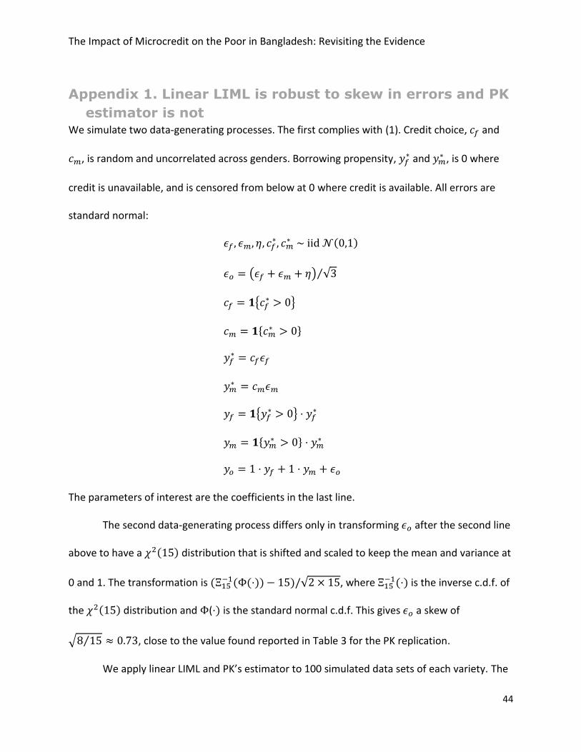
Appendix 1. Linear LIML is robust to skew in errors and PK

estimator is not We simulate two data-generating processes. The first complies with (1). Credit choice, and

, is random and uncorrelated across genders. Borrowing propensity, and

, is 0 where

credit is unavailable, and is censored from below at 0 where credit is available. All errors are

standard normal:

The parameters of interest are the coefficients in the last line.

The second data-generating process differs only in transforming after the second line

above to have a distribution that is shifted and scaled to keep the mean and variance at

0 and 1. The transformation is , where

is the inverse c.d.f. of

the distribution and ( is the standard normal c.d.f. This gives a skew of

, close to the value found reported in Table 3 for the PK replication.

We apply linear LIML and PK’s estimator to 100 simulated data sets of each variety. The


45

linear LIML regressions instrument and with and . The results confirm that, contrary

to the criticism in PK (2012) relating to weak instruments, linear LIML is consistent; and that the

PK estimator is more efficient when its assumptions are satisfied (left half of Table A-1). But

when the normality assumption is violated (right half), the PK estimator is inconsistent. This

again contradicts PK (2012)—or at least answers their argument that no one has proved that

their estimator is inconsistent.

Table A-1. Mean coefficient estimates, 100 simulations, with and without skew in second-stage error

y f y m y f y m

PK estimator 0.996 0.998 1.112 1.124

(0.025) (0.025) (0.030) (0.031)

Linear LIML 0.996 0.990 0.990 1.008

(0.046) (0.054) (0.050) (0.054)

True coefficients are 1.0. Standard deviations in parentheses.

Normal error Skewed error

The Impact of Microcredit on the Poor in Bangladesh Impact of Microcredit on the Poor in Bangladesh:...

Documents

Transcript of The Impact of Microcredit on the Poor in Bangladesh Impact of Microcredit on the Poor in Bangladesh:...