Moving The Nigerian Economy From Recession To Renaissance ...

NEAR EAST UNIVERSITYTHE GRADUATE SCHOOL OF SOCIAL SCIENCES
ECONOMICS DEPARTMENTMASTER OF SCIENCE ECONOMICS
MASTER’S THESIS
THE IMPACT OF FISCAL POLICY ON THENIGERIAN ECONOMY (1980-2012)
MUHAMMAD A. MUHAMMAD20124882
THESIS SUPERVISOR: ASSIT. PROF. DR. ERGIN AKALPLER
NICOSIA(2015)

ii
DEDICATION
To my lovely parents Alhaji Muhammad AwwalNuhu, HajiyyaHauwa Muhammad,Alhaji Muhammad Sani Ashraf Nuhu, HajiaAsabe Muhammad and late Officer MusaYawale. I dedicate this thesis to them as they are the most important people in my life.

iii
ABSTRACT
This study investigates the impact of fiscal policy on economic growth in Nigeria. The
data used is time series and span 1980-2012. Cointegration and Vector Error Correction
Model (VECM) is the approach used for data analysis. The series were tested to
determine their statistical properties using Augmented Dickey Fuller (ADF) and Phillip
Perron (PP). The series were found to be stationary or integrated of order one, that is, I
(1). Furthermore, a cointegration test was conducted. The result shows that, Trace Test
has 3 cointegration and Maximum Eigenvalue results indicates 2 cointegrating equations
of the series use in our model. The result of VECM shows that deficit financing,
domestic debt and government consumption expenditure are negative and significant
determinants of gross domestic product in Nigeria at 5% (α =0.05) level of significance.
However, external debt and government revenue are positive and statistically significant
determinants at 5% level of significance. The granger causality test shows some
variables having bi-directional causality, uni-directional causality and others without any
form of causality. The impulse response function shows that the variables have various
levels of shocks and innovation on itself and others. In trying to achieve macroeconomic
stability and sustainable growth in recent years, there has been excessive reliance on
public expenditure at different levels (Federal, State and local Government) that mostly
results to borrowing to finance fiscal deficits or complement internal resources. The
study suggests the need for conscious efforts to improve the quality of government
expenditure and the capacity to manage public resources.
Keywords: Fiscal Policy, Economic Growth, Co-integration, Vector Error Correction
Model.

iv
ACKNOWLEDGEMENTS
All praises and glories are for Allah (SWT) for his guidance, favor and bounties. MayThe peace and mercy of Allah be on our prophet Muhammad (SAW) and hisCompanions and those who follow him faithfully till the Day of Judgment.
I would like to thank my supervisor. Asst. Prof. Dr. Ergin Akalplerfor his continuousguidance, inspiration, support, opinion and encouragement in the preparation of thisthesis. My thanks are not enough for his continuous help.
I would like to express my special thanks to my family for their invaluable andcontinuous support throughout my studies and my life. They are: Abdurrahman Awwal,SalisuAwwal, Abdul-azisAwwal, Zakiyyu Sani Ashraf, Abdul-rashadAwwal, KhalidYussif, TahaSain Ashraf, Ahmed Sani Ahraf, Sadia, Hasia, Rahina, Ilham, Widad,Rashida, and Hamdiya may the Almighty Allah award them abundantly.
Furthermore, I would like to thank all of my friends for their endless support andencouragement in my life. Abdul-halim Ahmed, MustaphaHussainiGarinGabas,NuhuMuktarNuhu,Bashir AwwalAbubakar, Umar AminuAbdullahi, Muhammad Saeed Alyahaya (Erabil), Hydar Bashir Aliyu, MuhammadYasar, AbdulqayumAwwalAbubakar, ZainulAbideenJibril, Muhammad Sani Bello. MayGod bless and reward them abundantly.
My sincere appreciation goes to all the academic and non-academic staff of EconomicsDepartment, Near East University, especially, MrsTijenÖzügüney, Assoc.Prof. Dr.HüseyinÖzdeşer Head of Economic Department, MrsBehiyet, and Prof. Dr. Irfan Civcirfor their valuable and commendable helping hand towards the actualization of thisprogram.
I am indebted to Saadatu Musa Yawale (my fiancée) for encouraging me to studyabroad.May God reward her and the family abundantly.
My perpetual gratitude, appreciation and prayers go to those not mentioned but are inmy memory and those lost out of my memory. May God most profusely reward them all.

v
TABLE OF CONTENTSDEDICATION...................................................................................................................iiABSTRACT......................................................................................................................iiiACKNOWLEDGEMENTS..............................................................................................ivLIST OF TABLES...........................................................................................................viiLIST OF FIGURES ........................................................................................................viiiLIST OF ABBREVIATIONS...........................................................................................ixCHAPTER ONE ................................................................................................................1GENERAL INTRODUCTION..........................................................................................1
1.0 Introduction..............................................................................................................11.1 Background of the Study.......................................................................................31.2 Statement of the Problem.......................................................................................51.3 Objectives of the study...........................................................................................61.4 Research Questions ...............................................................................................61.5 Hypotheses of the Study ..........................................................................................71.6 Significance of the Study .........................................................................................71.7 Scope of the Study ...................................................................................................81.8 Organization of the Study ........................................................................................8
CHAPTER TWO ...............................................................................................................9LITERATURE REVIEW AND THEORETICAL FRAMEWORK .................................9
2.0 Conceptual Issues.....................................................................................................92.1 Tools of fiscal policy .............................................................................................122.2 Tools of Monetary Policy ......................................................................................132.3 Theoretical Review ................................................................................................142.4 Empirical review ....................................................................................................172.5 Theories of fiscal policy.........................................................................................222.6 Theoretical Framework ........................................................................................23
CHAPTER THREE .........................................................................................................28OVERVIEW OF FISCAL REGIMES AND PERFORMANCE IN NIGERIA ..............28
3.1 Fiscal Policy and Economic Outlook in Nigeria....................................................283.2 Performance of Domestic Debt in Nigeria...........................................................33

vi
3.3 Reason for Rising Domestic Debt Profile in Nigeria..........................................343.4 Nigeria's Debt Management Strategies ..................................................................353.4.2 Debt-Equity Conversion .....................................................................................373.4.3 Debt Forgiveness ..............................................................................................37
METHODOLOGY AND DATA ANALYSIS ................................................................384.2 Definitions of Variables ....................................................................................394.3 Technique of Analysis ...........................................................................................414.3.1 Unit Root Test for Stationarity (ADF and PP) ..............................................414.3.2Cointegration Test................................................................................................424.3.3Granger Causality Test.........................................................................................434.5. Empirical Results ..................................................................................................444.5.1 Unit Root Test of Stationarity..........................................................................444.5.2 Johansen Cointegration Test ...........................................................................45
CHAPTER FIVE .............................................................................................................57SUMMARY OF FINDINGS, CONCLUSION AND POLICY RECOMMENDATIONS..........................................................................................................................................57
5.1 Summary of Findings..........................................................................................575.2 Conclusion ..........................................................................................................585.3 Policy Recommendations ..................................................................................58
BIBLIOGRAPHY............................................................................................................60APPENDIX I: VECTOR ERROR CORRECTION MODEL ESTIMATION................66APPENDIX II: IMPULSE RESPONSE (Figure) ...........................................................70APPENDIX III: GRANGER CAUSALITY....................................................................73APPENDIX IV: DATA ...................................................................................................75APPENDIX V: FIGURE 3 ..............................................................................................77APPENDIX VI: FIGURE 2 .............................................................................................78APPENDIX VII: FIGURE 1............................................................................................79

vii
LIST OF TABLES
Table 4.1 ADF and PP Unit Root Tests for Stationarity 53
Table 4.2(a) Johansen Co-integration Test (Trace Test) 55
Table 4.2(b) Johansen Co-integration Test (Maximum Eigenvalue) 56
Table 4.3 Vector Error Correction Model Estimated Result 58
Table 4.4 Pairwise Granger Causality Test 59
Table 4.5 Impulse Response 60

viii
LIST OF FIGURES
Figure 1 Real GDP and Fiscal Deficit Trend (% of GDP) 37
Figure 2 GDP, EXD and DMD Relationships (% of GDP) 38
Figure 3 Real GDP and Government Revenue (% of GDP) 39

ix
LIST OF ABBREVIATIONS
ADF Test Augmented Dickey-Fuller test
AIC Akaike Information Criteria
DF Deficit Financing
DMD Domestic Debt
ECM Error Correction Model
ECT Error Correction Term
EXD External Debt
GCE Government Consumption Expenditure
GDP Gross Domestic Product
GRV Government Revenue
IMF Internal Monetary Fund
PP Test Phillips-Perron test
RGDP Real Gross Domestic Product
SIC Schwartz Information Criterion
VAR Vector Auto Regressive
WDI World Development Indicators

1
CHAPTER ONE
GENERAL INTRODUCTION
1.0 Introduction
Nigerian government over the years had consistently embarked on diverse
macroeconomic policy options in order to direct the economy on the path of growth and
development. One of the measures or policy option the government frequently used, is
the fiscal policy. Fiscal policy refers to a deliberate attempt by the government to
manipulate its expenditure, taxes and public debts to achieve macroeconomic objectives
of the governments among which are economic growth. Several economic problems
bedevilled the growth and development of the economy which may be identified as high
rate of unemployment, inflation, under capacity utilization in industrial sector, poor
infrastructures and a host of other problems which necessitated the frequent government
intervention in the management of the economy through its fiscal policies.
Despite huge amount of revenues accruing to the federal government of Nigeria through
the sale of crude oil and improved tax system, successive government borrowing both
internal and external to finance ever increasing government expenditure and direct
government involvement through various public enterprises, an overview of the Nigeria
economy for the past two decades shows that inflation still remain high in Nigeria,
unemployment has increased to an unimaginable size, economic growth has also been

2
little until 2000s when it start improving significantly, the balance of payment also faces
pressure over the period.
Several fiscal measures have been implemented and given the importance of fiscal
policy in macroeconomic management in Nigeria, economic growth has not accelerated.
The growth of the economy has been sluggish although recently improved, that does not
translate in the living standard of the populace as poverty level is increasing by the day,
youth unemployment reaching unprecedented level, inadequate and mal functioning
infrastructures. It is therefore very important to examine the effects of some fiscal policy
instrument on the growth of the Nigerian economy over the years under study in order to
access their contribution or otherwise.
Exploration into the literature has also shown that, fiscal policy is widely recognized as a
strong tool for improving economic growth in most economies of the world, though the
Nigerian experience is tending to suggest otherwise. A number of studies have examined
the empirical relationship between fiscal policy and economic growth. The results of
these studies are varied. Studies such as that of Barro& Martin (1990);
Glomm&Ravikumar (1997); Genetski& Chin (1978); Eusterly and Rebelo (1993) have
examined the relationship between some fiscal policy variables (taxation and public
expenditure) and economic growth. Their statistical result is not unanimous, while some
studies found out that taxes have long term influence on growth rate, others found no
significant effect. Hence, the need for other studies that will try to find out whether fiscal
policy have any substantial impact on Nigeria’s economic development in order to clear
the uncertainties and the counter results of the previous studies.
Moreover, given the nature and importance of the relationship between fiscal policy and
the gross domestic product, the study becomes necessary in Nigeria, where output and
capacity utilization have suffered rapid fluctuations. Since the public desires is to
increase total expenditure in the economy through its fiscal policy which can either
increase its spending or reduce taxes in ensuring stability in the economy, it is therefore
the researcher’s interest to investigate the impact of such fiscal policy instruments as;
government revenue, government expenditure, external and internal debt and deficit
financing on the growth of the Nigerian economy.

3
1.1 Background of the Study
Fiscal and monetary policies are important instruments use to achieve stable and viable
macroeconomic environment in a drive towards the achievement of economic growth
and development of economies especially developing countries. It is evident that in a
fast integrated world, macroeconomic fluctuations with political instability and
doubtfulness hampered long term growth, development and welfare (Adefeso and
Mobolaji, 2010; Hnatkovska and Loayza, 2005). As a result economies around the globe
keep fine tuning their policies to place their economies on growth path in a sustainable
manner.
The macroeconomic policy objectives that economies seek to achieve include price
stability, economic growth, full employment and balance of payments. In addition,
developing economies also seek to achieve exchange rate stability and equitable
distribution of income or resources. This has been an economic policy priority of
advance and developing countries because of the degree of exposure of macroeconomic
variables to volatility in the face of globalization (Zhattau, 2013; Omitogun and Ayinla,
2007). To gain macroeconomic policy targetsit requires the use of fiscal and monetary
policy instruments.
The main fiscal policy instruments include public expenditure and tax (Wosowei, 2013).
The fiscal policy is crucial for the performance of an economy. This is because the
ability of the government to collect tax and use it to provide public goods enhanced
economic and social activities that propel economic growth and development. This role
played by government in growth process also significant for the performance of the
private sector. For instance, government spending can provide the incentive for private
sector growth on the one hand, though on the other hand it can crowd-out of the private
sector scarce resources in a situation where budget deficits leads to competition for
scarce financial resources from the banking sector as the government seeks to finance its
deficit. This can be harmful to the growth of the economy by outweighing any short-
term benefits of an expansionary fiscal policy. Therefore, determining and ensuring a
balance in the management of fiscal regime (in addition to the monetary policy) is
fundamental for its effectiveness. While it is necessary to generate enough income to

4
meet up with government expenditure outlays and support growth driven activities, it
should not be in a manner that will affect the level of financial resources required by the
private sector to invest and boost industrial activities.
The Nigerian economy over the years has been characterised by fiscal policy instability
(Akani and Osiniwo, 2013). The level of fiscal instability has been a function of
fluctuations in government revenue largely because of the heavy dependence of the
economy on crude oil revenue that is subject to international market price volatility. To
reduce the extent of such impact the monetary authority (Central Bank of Nigeria) is
compelled to implement policies that act to neutralize and in some instances leads to
further macroeconomic instability (Vincent et al., 2013; Obiyeluaku, 2006). Beside the
fact that Nigeria is one of the developing economies, one of its major economic
challenges is that it is susceptible to volatile macroeconomic environment constrained by
external terms of trade shocks and reliance on crude oil export. The focus on oil has
hampered the diversification of the Nigerian economy and Industrialization.
Nigeria discovered oil in 1956 but began to export oil in 1958. Beginning from early
1970s oil has become the prevailing factor in Nigerian economy and the revenue from it
is the major source of government income. The oil price volatility in the international
market has had its share on fiscal instability in Nigeria which largely has channelize its
effect to the rest of the economy with fundamental effect on government revenue and
provision of public goods. The recent oil price decline that started mid-last year with the
price above US$100 now sale for around US$50 (January, 2015). The effect of such
decline is oil price is usually felt on real exchange rate and growth performance. More
worrisome, is the fact that the Federal Government of Nigeria budget of 2015 fiscal year
is predicated on US$65 per barrel while actual price of crude oil is around US$50. This
indicates a deficit of about US$15 and still counting.
The deficit financing has remained unyielding in Nigeria because of the public sector’s
lacking the power or unfitness to manage her fiscal abreast in a sustainable manner
(CBN, 2014). Since the forceful oil price fall of early 1980s including the contemporary
oil price decline challenge, fiscal policy management in Nigeria has lost the desirable
characteristics required for its effectiveness as a tool for aggregate demand management

5
(Medee and Nenbee, 2012). Ezeoha and Chibuike (2005) observed that government at
all levels (three tiers) are fiscally reckless and more often than not contradicts the
fundamental monetary policy objective of price stability. The consequence has been the
potential for destabilizing the macroeconomic environment that can retard economic
productivity and development. Therefore, the search for viable and stable
macroeconomic environment through sound fiscal and monetary policies cannot be
overemphasized.
The quest to finance fiscal deficit usually results in public debt policy to fill the resource
gap arising from the inadequacy of non-debt national and international financial
resources. This is required to implement public policies and development programmes
of government. In view of this, the Nigerian government overtime has resorted to
procuring loans from both internal and external sources to supplement non-debt sources
of financing growth. The use of debt instruments accordingly, has provided mixed
results (Bamidele and Joseph, 2013; Vincent et al., 2012). Debt over hang became a long
economic problem that confronted Nigeria in 1980s and 1990s, until debt relief or
forgiveness that was granted in the early 2000s.
1.2 Statement of the Problem
The Nigerian government have made effort through policy measures to address fiscal
challenges (external and domestic), this has remained intractable and persistent with its
adverse effect on macroeconomic fundamentals. In developing economies like Nigeria,
borrowing from international financial institutions and Central Bank to finance sizeable
portion of the deficits contribute to liquidity and inflation (Bamidele and Joseph, 2013;
Cohen, 2005). This is because rather than spending the borrowed money on capital
expenditure such that has the capacity to improve standard of living of which in turn
may improve the country’s economic growth, such borrowed money is used on
unproductive ventures (Iyeli and Ijomah, 2013; Iyoha, 1999). This has led to situations
where expenditure could not be cut back or cut short, resources could not be raised for
fear of adverse effects, and greater deficits fuelled more inflation on one hand, while
debt increase pose another threat of high debt service on the economy.
6
The impact of fiscal deficit on macro-economic aggregates depends or reckon on the
financing techniques (Inflation tax). Also the use of expansionary monetary policy often
leads to inflation while domestic borrowing inevitably or unavoidable leads to a credit
squeeze or pressure through higher interest rates or through credit allocation (Easterly
and Robello 1994 Sowa, 1994).
However, though there are recent studies on the impact of fiscal policy on economic
growth in Nigeria with particular reference to the impact of fiscal deficit and debt
(Bamidele and Joseph, 2013; Akani and Osiniwo, 2013; Vincent et al., 2013), there is no
consensus on the subject matter. Some have argued that the level of economic
development and the fiscal structure of Nigerian economy compound the problem
(Medee and Nenbee, 2012; Ndekwu, 1996). Besides, some studies have advanced in
characterising the implications of alternative sources and composition of deficits
spending without investigating whether fiscal deficit lead to economic growth (Nathan,
2012). Thus, studies on fiscal policy instruments seem to have divergent or different
views.
1.3 Objectives of the study
The objectives analyze the impact of fiscal policy on the Nigerian economy (1980-
2012).
The specific objectives are:
(i) To examine the impact of fiscal policy instruments on Nigerian economy.
(ii) To determine the causal relation between fiscal policy and economic
performance in Nigeria and
(iii) To analyze the trend of fiscal policy instruments in Nigeria.
1.4 Research Questions
The study addresses the following questions:
(i) What is the impact of fiscal policy on Nigerian economy?
(ii) What is the impact of fiscal policy instruments on Nigerian economy?
(iii) What is the causal relation between fiscal policy and economic performance in
Nigeria?

7
(iv) What is the trend of fiscal policy instruments in Nigeria?
1.5 Hypotheses of the Study
Hypothesis is tested to know whether fiscal policy instruments have over the years,
impact positively or negatively on economic growth. Also, to test whether fiscal policy
instruments are effective and efficient source of managing development in Nigeria. The
hypotheses that this study seeks to test are stated in null form below:
(i) H0: β0< 0; Fiscal policy does not affect economic performance in Nigeria
(ii) H0: β0< 0; Fiscal policy instruments does not affect economic performance in
Nigeria.
(iii) H0: β0< 0; There is no causal relationship between fiscal policy and economic
performance in Nigeria.
1.6 Significance of the Study
The aim of every government is to ascertain the security of life and property and fast
tracteconomic growth and development. This is even to a greater extent important in
Nigeria where the citizen looks up to government for the provision of most of its basic
needs including developing human capital. To achieve this, government directly or
indirectly mobilize long term fund (internally and externally) for its development
programmes, to achieve high and prolong level of economic growth.
This study recognized the important role of debt financing over the years. However, the
quest for reducing debt financing instruments because of its impact on the economy for
non-debt in recent times has not been properly covered in most studies.
Therefore, the study is significant in a number of ways. Looking at the range and the
procedure adopted, it’s observed that, the result of the present study will make a
meaningful policy preparation and carrying out in the development of an economic
growth in Nigeria. It will also, provide evidence for researchers with interest on the
subject field matter.

8
1.7 Scope of the Study
The study examines the impact of fiscal policy on economic growth in Nigeria covering
the period 1980–2012. The specific fiscal instruments of interest are rate of deficit
financing and debt (external and internal).
1.8 Organization of the Study
To achieve the objective of this study, the work is organized into five chapters. Apart
from chapter one which this part conclude as introduction, Chapter two is literature
review. The chapter provides conceptual, empirical and theoretical review as well as
theoretical framework and review previous studies. Chapter three is overview of fiscal
regimes and performance in Nigeria. Chapter four this chapter describes source and type
of data and methods of data analysis and empirical analysis and discussion of result.
Chapter five is summary, conclusion and recommendation.

9
CHAPTER TWO
LITERATURE REVIEW AND THEORETICAL FRAMEWORK
2.0 Conceptual Issues
Fiscal policy refers to the deliberate attempt of government policy to manipulate its
expenditure and the raising of gross or tax revenue through taxation and other sources
and determining on the level and figure of consumption for the purpose of regulating
economic activities (Munogo, 2012). It can also be seen as a policy whereby the
government uses its expenditure and revenue programmes to produce worthy effects and
prevent unworthy effects on national income, production and utilization. According to
Jhingan, 2003 fiscal policy is a deliberate spending and taxation actions undertaken by
government in order to control inflation, achieve economic growth, and to bring about
nation’s output and employment to desired levels.
Fiscal policy can be seen in two different ways that is discretionary and non-
discretionary. The discretionary fiscal policy is a deliberately attempt or measure by the
government or its agencies to influence the economy in a desired direction in order to
achieve macroeconomic objectives through taxes and government expenditure. On the
other hand, non-discretionary fiscal policy we mean the actions that occur
automatically without any deliberate attempt but due to the existence of automatic built-
in stabilizers within the economy such as, unemployment benefits and progressive tax
system. Since this non discretional fiscal policy tends to help the economic
automatically it’s refer to as automatic built-in stabilizers. There is need for government

10
to stabilize the economy, specifically by making some adjustment to the level and
allocations of taxes and expenditure. Federal taxation and expenditure policies are
designed to level the business cycle and achieve full employment, price stability and
sustained growth of the economy.
Fiscal policy can also be expansionary and contractionary. An expansionary fiscal policy
is desired to stimulate aggregate demand thereby increasing economic activities in order
to reduce or fight depletion, unemployment and to achieve economic growth. This
policy is always adopted when government wants to pull the economy out of recession.
While contractionary fiscal policy refers to the policy designed by the government to
reduce aggregate demand in order to fight inflation and correct balance of payments
problem.
The main objectives of fiscal policy according to Anyanwu and Oaikhenan (1995) are
generation of significant revenue for the government with which she can provide other
services that benefit the entire society diversification of revenue sources away from
crude oil-based revenues, deduction in the tax burden on individuals and corporate
bodies; maintenance of economic equilibrium, particularly to control inflationary
pressures, speed up economic growth, decrease Balance of Payments deficits, and yield
increased employment.
Fiscal deficit it is the disruption within the government’s total expenditure and the total
of its revenue receipts and non-debts capital receipts, (Buhari 1994). Which exemplify
the total amount of borrowed funds demand by the government to totally meet its
spending. It can also be defined as the surplus of total expenditure including loans net of
payments over revenue receipts and non-debt capital receipts. It also indicates or
suggests the total borrowing of the government, and the growth or increase to its
outstanding debt.
Debt on the other hand is produce by the act of borrowing. It can be defined according to
Oyejideet al (2004) as the resource or money use by an establishment or governing body
that is not contributed by its owner and does not in any other way belong to them. It is a
financial obligation represented by a financial tool or other formal equivalent. External
debt therefore can be defined as the resources of money in use in a country that is not

11
yield internally and does not in any way come from local citizens whether corporate or
individual. Oke (2012) defined external debt as the total amount of money at any given
time disbursed or pay out and outstanding or unpaid contractual indebtedness of
residents to pay interest, either with principal or without principal.
When a government borrows, the debt is a nation debt. Nation debts internal and
external are debts receive by government through borrowing in domestic and
international markets in order to finance domestic investment. Therefore, national debt is
observed as all claims against the government maintain by the private sectors of the
economy or by the foreigners, whether interest aim or not, less any claims held by the'
government against the private sectors and foreigners (Anyanwu,1999). Public debt can
be internal or external: internal debt can be described as when debt is owed or held by
the subject of the indebted government. Whereas, international debt refers to unpaid
portion of external resources acquired for developmental purposes and BOPs supports,
which could not be repaid when they cut down payable (Salawu, 2004). In other words,
external debts are debts owed by a country to institutions or countries abroad, that is, the
creditors are foreigners in which case, its services and repayment will mean drainage of
national resources in favor of the foreigners.
One of the most important objectives of macroeconomic policy in recent years has been
the rapid economic growth of an economy. Economic growth can be defined or seen as
the process whereby the real per capita income of a country increases over a long
duration of time. Economic growth is measured by the increase in the total amount of
goods and services produced in a particular country. A growing economy produces more
goods and services in each successive time duration. In its wider aspect, economic
growth implies raising the standard of living of the people and reducing inequality of
income distribution (Jhingan, 2003).
The relationship between government expenditure and economic growth has continued
to generate series of debate among scholars. Some scholars argued that increase in
government socio-economic and physical infrastructure encourages economic growth.
For example, government spending on wellness and education raises the productivity of
labour and increase growth of national output. Likewise expenditure on infrastructure

12
such as roads, communications, power, etc., enhance private sector investment, reduces
production costs and gainfulness of firms, thus, raising economic growth.
Overall, the Keynesian revolution changed the meaning of fiscal policy moving it away
from the tax or revenue side of the budget to include both revenue and spending. For the
Keynesians, fiscal policy refers to the manipulation of taxes and public spending to
influence aggregate demand which also include its stabilization role.
2.1 Tools of fiscal policy
A rational government basically uses government expenditure taxes and subsidy as good
tools to achieve its stated goals of macroeconomic variables through the manipulation of
fiscal policy.
1. Government Expenditure: - If government wants to embark on an expansionary
fiscal policy in order to stimulate the aggregate demand, it will increase its expenditure.
This is usually adopted during the period of recession when there is high rate of
unemployment, low demand and decrease in output of goods and services.
On the other side if the objective of the government is to embark on a contractionary
fiscal policy it will decrease its expenditure and increase taxes in order to reduce the
aggregate demand. This is usually adopted during the period of inflation or when
balance of payment is in deficit.
2. Taxation: - Tax is another tool or instrument used by the government in order to
achieve the stated macroeconomic goals. If the government wants to embark on an
expansionary fiscal policy taxes could be reduced and as a result of reduction in taxes,
money is made available in the hands of individuals and this will result to an increase in
demand for goals and services. This will stimulate producers or manufacturers to hire
more factors of production and this will raise the level of output. This policy is usually
adopted during the period of recession and low aggregate demand.
On the other hand, if the government wants to embark on contractionary fiscal policy it
will increase taxes, this will in turn lead to a decrease in the purchasing power of
individuals and aggregate demand will also fall. This policy is adopted in time of
inflation or when the country’s balance of payment is in disequilibrium.

13
3. Government Subsidy: - Government should subsidize when it is embarking on an
expansionary fiscal policy. This is usually put into use when there is unemployment.
For a contractionary fiscal policy, the government should reduce its subsidy. This is
usually done during the period of inflation and during the period of balance of payment
deficits.
2.2 Tools of Monetary Policy
The Federal government of Nigeria find it very difficult to control inflation and also
influence the country output as well as employment directly instead it uses the monetary
policy tools which are as follows:
1. Open Market Operations
Open market operations refer to sale and purchase of securities in the money market by
central bank, when prices are rising and there is need to control them, the central bank
sells securities. The reserves of commercial banks are reduced and they are not in a
position to lend more to the business community. Further investment is discouraged and
the rise in prices is checked. It is expansionary or contractionary.
2. Bank Rate
The bank rate is the minimum lending rate of the central bank at which it rediscounts
first class bills of exchange and government securities held by the commercial banks.
The rate influences the other interest rates in the economic activities within a given
economy.
3. Funding
This refers to the conversion of short-term government securities. For example, treasury
bills (short-term liabilities) could be converted to long-term securities(such as bonds) if
the Central Bank feels that the condition of the economy has not yet improved for the
short-term loans to be repaid. If inflation persists, short-term securities may be converted
to long –term ones.

14
4. Reserve Ratio
Every commercial bank is required by law to maintain a minimum percentage of its
deposits with the central bank, the minimum amount of reserve with the central bank
may be either a percentage of its time and demand deposits separately or of total
deposits, whatever the amount of money remains with the commercial bank over and
above these minimum reserves is known as the excess reserves
2.3 Theoretical Review
The Keynesian theory advocates the use of fiscal policy to offset imbalances in the
economy. According to Keynes, a government should use fiscal policy to stimulate an
economy slowed down by recession through deficit, which means it should spend more
than what it collects from taxes. On the other hand, to slow down an economy that is
threatened by inflationary pressures, government should increase taxes or cut
expenditure to create a budget surplus that would act as a drag on the economy
(Grossman 1987). Stabilization policy requires that policy makers can determine feasible
targets and can effectively control the instrumental variables for which the government
seek desirable values.
The continual inclusive opinions regarding the role of government in managing the
economy using fiscal policy lies in two dominant theoretical views. The first is the
Keynesian perspective, which makes up the subject that government can play a major
role in determining the level of national income. The alternative is the Ricardian
perspective, which states that, the level of national output is basically neutral to
government policy. The effectiveness of fiscal policy will therefore depend very much
on which view persists (Chamberlin and Yueh, 2006). The difference between the
Keynesian and the Ricardian view of the world comes down to the type of consumption
function that is used, while the Keynesian model states that expansion of government
expenditure (expansionary fiscal policy) accelerates real GDP, endogenous growth
models do not allocate any significant role to government in the growth process, but
Barro and Sala-Martin (1992); Easterly and Rebelo (1993) emphasized the importance
of government intervention in economic activities to enhance economic growth.

15
The literature on fiscal federalism provides guidance on how expenditure assignment
could be optimally designed on the grounds of distribution efficiency, flexibility,
independence and accountability. Over a period of time, government intervention has
increased in absolute and relative terms, particularly in developing countries of the
world. This growth in public sector size has been attributed to some reasons (according
to Wagner’s hypothesis), which involves increasing income, elasticity of voters needs
for public goods, comparative price changes effects such as depressions, interest group
needs for instance, public sector employees productivity, redistribution, motivations as
well as centralization of government activities (Musgrave and Musgrave 2005;
Grossman, 1992).
For instance, Barro (1990) and Diamond (1990) formally endogenized government and
the rate of growth and savings. From an allocating view of point, an increase in public
consumption leads to capital formation or private consumption. Some development
economists of the structuralize school opined that some categories of government
expenditures are necessary to overcome constraints to economic growth (Chenery and
Syrguin, 1975). From the foregoing, it is clear that if fiscal policy is used with
circumspection and synchronized with other measures, which will probably smoothen
out trade cycles and lead to economic growth and stability.
Governments directly and indirectly influence the way resources are used in the
economy. Fiscal policy that increases total demand directly through an increase in
government expenditure is typically called expansionary or sloppy. By contrast, fiscal
policy is often considered contractionary or “tight” if it reduces demand via lower
spending (Horton and El-Ganainy, 2009). Horton and El-Ganainy (2009) observed that
besides providing goods and services, the objectives of fiscal policy differ. In the short
run, governments may emphasis on macroeconomic stabilization. In an oil-producing
country, fiscal policy might aim to moderate pro-cyclical spending; moderating both
bursts when oil prices rise and painful cuts when they drop.
Richard et al., (2009) noted that fiscal policy affects national output, the country’s
capacity to produce goods and services and the distribution of income. In the short run,
changes in expenditure or taxing can alter both the magnitude and the pattern of demand

16
for goods and services. With time, this national output affects the allocation of resources
and the productive capacity of an economy through its influence on the returns to factors
of production, the development of human resource, the allocation of capital expenditure
and investment in technological breakthrough. Fiscal policy together with monetary
policy according to Omitogun and Ayinla (2007) and Adeoye (2006) is the most
important means of regulating the rate of inflation in an economy and preventing or
controlling depression. They noted that when there is economic recession or depression,
government usually plans budget deficit, popularly known as expansionary fiscal policy.
Grayet al., (2007) asserts that government can use fiscal policies to reduce the demand
for goods and services. It can prevent depressions by increasing expenditure, while the
rate of inflation can be controlled by decreasing expenditure. Fiscal policy determines
tax rates, which in turn influence the level of expenditure by influencing the total
amount of money people have for consumption expenditure. Government can also
decrease or increase its own spending to manage inflation and depression.
Fiscal policies that increase the deficit will result in future taxes being higher than they
otherwise would have been, but, depending on the policies’ effects on incentives for
investing in human or physical capital, they might also raise future living standards.
(Horton and El-Ganainy, 2009).
Blinder (2006) argued that views on the use of discretionary fiscal policy as a tool for
macroeconomic stabilization have undergone changes since the early 1960s, when it was
generally viewed that discretionary fiscal policy was effective and desirable for taming
the trade cycle, and that fiscal policy was the most important tool with which to conduct
stabilization policy. He concluded that the weight of the evidence supports the view that
both temporary and permanent tax changes do affect consumption spending. In the final
analysis, argued that monetary policy should be relied upon as the primary policy tool
for macroeconomic stabilization, but that discretionary fiscal policy can play an
important stabilization role under unusual circumstances. When a recession is unusually
long or when a short-term nominal interest rate approaches zero, then it is appropriate to
supplement monetary policy with fiscal stimulus.

17
2.4 Empirical review
The empirical literature is rich of studies on the impact of fiscal policy on economic
growth ranging from countries with undeveloped economies to developed economies,
with diverse methodologies. It is evident from the wide range of previous studies that the
results are mixed and varies upon the economic development activity and stability of the
studied country. For instance, Adam and Bevan, (2004) using panel data of 45
developing countries analyzed the relationship between fiscal deficits and growth. The
study revealed a beginning effect of the deficit around 1.5 percent of GDP. This
threshold tangled a change in slope and a change of sign in the relation irrespective of
the budget category. This studies framework states that a non-steady point economy,
short range funding might be growth-enhancing. This result points to the fact that the
activity of economic growth has impact on deficit financing. This result is not
appropriate for an economy like Nigeria. Also, it fails to capture fiscal dynamics of
economies around the world.
Brauninger, (2002) examined the interactions between budget deficit, Public debt and
endogenous growth. The study found that a fixed deficit ratio by the government holds
below an unfavorable degree. Brauninger concluded that there is no equilibrium if the
deficit ratio surpasses the unfavorable level. Moreover capital growth declines
incessantly and capital itself is driven down to zero in finite time.
De Castro, (2004) took Spain as a sample and investigated the effect of Fiscal Policy, he
found that a shock to government expenditure boosts Gross Domestic Product, private
consumption and investment, accompanying with a positive multiplier close to one in
the short term and a negative multiplier in both the medium and long terms. These
studies largely focus on steady state growth but economics are largely dynamic and
cannot he explain by static models. Studies in Europe may not also explain fiscal
dynamics of African countries like Nigeria.
18
Benos, (2004) investigated the OECD countries revealing a V-shaped relationship
between government expenditure on social amenities and energy. On the other hand a U-
shaped relationship with growth was found among other variables namely: the rate of
per-capita growth, public expenditures on social protection, social assistance and
transportation and communication. Moreover the effect of growth from public spending
on education and social expenditure is stronger, the poorer the country is. In contrast the
contradictory is true for expenditure on health. The study also showed that a positive
effect exists between budget surplus and growth.
Cohen, (2005) attempted to find the extent of attribution of the debt crisis of the 1980’s
to the growth slowdown of the 1990’s. Moreover measure what could be a suitable debt-
to-export target. This study found that the debt crisis of the 1980’s played a significant
role in leading to the growth slowdown of Latin America and Africa in the 1990’s
period. Exposing a debt-to-export ratio of between 200 percent and 250percent was a
strong signal for an approaching debt crisis. This high percent stressed the need of
African countries to a debt to export ratio to be brought to 198%. Fiscal dynamics of
economies are not time bound and the effect may vary depending on the nature of the
shocks. Thus, the 21 crisis may be different from 1980s or 1990s crisis.
Edward (2001) Using a panel data of 104 LDCs for three periods (1970-1979, 1980-
1989, 1990-1998), investigated to what extent economic growth may be adversely affect
from the uncertainty in the annual debt service payments, specifically for heavily
indebted poor countries. He justified that the large time to time fluctuations in debt
service payment make it difficult for the governments of poor countries to precisely
expect the sufficient amount of resource available to carry out economic reforms.
Edward suggested a sweeping debt relief initiative may help contribute to regain these
economies growths. This can be reached by reducing uncertainty with respect to debt
service payments assuming it will increase the effectiveness of future government
policies and therefore providing the private sector with positive signals regards their
future possibilities of profitability. The use of panel data by the study may not provide a
country specific effect as a country specific study may be preferable.
19
Pattillo and Ricci, (2004) investigated the quantitative effect of debt on economic
growth using multiple regression analysis. Their findings stated that debt and economic
growth presented an inverted U-shaped relationship. Accordingly a positive impact on
economic growth is likely to be when countries accept more foreign capital and start
borrowing. In addition, a negative contribution was shown from debt to economic
growth over the period from 1960’s to 1970’s. In a similar fashion, the study used panel
data and could not provide country specific results thus the need for a disaggregated
model.
Grossman and Elhannan, (1990) Investigated the impact of Jordan’s external
indebtedness on its economic growth. The results revealed the existence of a positive
relationship between external debt and economic growth below 53 percent of GDP. In
cases where the debt increases beyond this level, its effect on the Jordanian economy
turn out to be negative significant. The threshold determined in Jordan cannot be
universal due to country specific examination.
Kraav and Vihani (2004) from 1968 to 1998 examined the ways through which debts
affects growth by applying on 60 developing countries. Non-linearity was shown as
evidence to the relationship between sources of growth and the level of debt of the
country. TFP growth had a positive influence on growth with little debts levels in
contrast had a negative influence at great debt levels. In addition, the existence of a
negative effect from physical capital on TFP growth was shown. Conclusions were that
boosting both capital accumulation and productivity growth will make to reduce debt
level and therefore will give to growth increment.
Munongo, (2012) covering the time period from 1980 to 2010 of Zimbabwe’s economy,
Munongo investigated the efficiency of fiscal policy in encouraging economic growth.
In order to take in consideration of short-run dynamics Error-correction models were
applied. The results indicated that both government consumption and tax income
positively influenced significantly Zimbabwe’s economic growth during the period of
coverage. In contrast capital expenditures had a negative effect accompanied with a
long-run relationship. Zimbabwean economy has experience some level of crisis in

20
recent times with high level of instability politically and economically. This seems to
affect economic fundamentals in Zimbabwe.
Onah, (1994) by selecting eight African countries examined the affection of external on
their GNP growth prospects. Onah summed up his results that, the extensive and
significant increments in these countries’ GNP are still consistent with increments in
debt. The debt ratio to GNP for all countries becomes large to tolerate at 5 percent
increment in debt and more. Moreover improvement of the growth of the economics can
be achieved by a reduction of debt.
Essien and Onwioduokit (2002) found that the degree of responsiveness of growth to
external finance in Nigeria was elastic. They advised to place appropriate debt
management strategies in order to give feasibility studies for plans financed by
externally injected resources invested in productive ventures.
Nathan (2012) investigated the causality between selected variables namely: exports,
fiscal deficits and money supply as a representation of analyzing the impact of economic
policies on economic growth of the Nigeria in a time span between 1970 and 2010. Co-
Integration, Error Correction Model (ECM) and a Two Hand Recursive Least Square
tests were the test applied on the data. The objective was to explore the influence of the
selected variables on the relative effectiveness of Nigeria’s economies’ past
implemented fiscal policies. Outcomes of the study showed evidence that a significant
causal relationship between gross domestic product (GDP) and both exports and fiscal
policies exists. The policy variables employed in this study did not capture government
income and consumption which are important indicators of fiscal policy. There is need
to examine the effect of such variables on the performance of the economy.
Iyeli and Ijomah (2013) applied a co-integration and Error Correction Model technique
to investigate the influence of selected fiscal policy variables on Nigeria’s economic
growth between the period 1970 and 2011. A long run relationship between economic
growth and the selected variables existed in the outcomes of the study.
Vincent et al., (2012) studied the bond between economic fiscal deficits and economic
growth. They applied the analysis over a time period from 1970 to 2006. A modeling
technique that incorporates co-integration with structural analysis was used. The studies

21
outcomes showed that fiscal deficit influences economic activity negatively if a lag is
accompanied in the system. Moreover a one percent rise in fiscal deficit is expected to
decrease economic growth by 0.023 percent. Also existence of a strong negative
relationship between economic growth and government expenditure was shown in the
analysis.
Zhattau, (2013) argued that economic growth is a powerful engine for generating long-
term standard of living and that fiscal policy has been identified as a means of
generating growth. Taxation as a major source of government revenue as well
government expenditure is an important channels of transmission between fiscal policy
and growth. He employed a descriptive method to review the effect of fiscal policy in
Nigeria. The study revealed that there are various challenges facing fiscal policy and tax
implementation in Nigeria and that an appropriate method of tax implementation will
increase the revenue of the country thereby accelerating economic growth. The stud
submitted that efficiency of tax system is not just a matter of appropriate tax laws hut
also the efficiency and integrity of tax administrators.
Wosowei (2013) investigated the relationship among macroeconomic performance in
Nigeria and its fiscal deficit for the period span from 1980 to 2010, with a view to define
the impact on macroeconomic aggregates from fiscal deficits, and whether fiscal deficit
had led lo economic growth in Nigeria. He used OLS in analyzing the model. The
findings showed that fiscal deficits even though that it met the economic a prior in terms
of its negative coefficients so did not significantly affect macroeconomic productivity.
The result also revealed a bi- causal relationship between governmental balance deficit
and GDP, government tax, and unemployment, while a uni-causality between economic
deficit and government expenditures and inflation. This study used a static model and
requires some form of verification using a dynamic model approach including the causal
linkages.
From the various past studies in which analyzed the linkages between economic growth
and the fiscal policies it is assured that the results are in a variety of outcomes. Some
studies found a negative relationship while others found a positive in contrast.

22
2.5 Theories of fiscal policy
The fiscal policy analysis in the light of macroeconomics is founded by some theories.
In particular, we have Keynesian and Ricardian Equivalence theories. The mechanism
behind the fiscal policy is clarified by the Keynesian income-expenditure method. The
fiscal policy according to Keynesians has significant cause on income, employment and
productivity in the short term without money supply. It asserts that aggregate demand is
a determinant of output. An increase in government expenditure will reflect a cause and
surge in domestic income. As internal income increases, imports will also increases and
finally decrease the surplus in the trade cycle. Also, the Keynesians open economy
model asserts that a casual relation runs from budget deficit to aggregate demand.
Specifically rise in budget deficit will increase the interest rates as acompensation of the
loss and a source of fund. Therefore increases the capital inflows thereby increasing the
demand on the local currency (Barro. 1989).
Enders and Lee (1990) opined that public debt is as crucial as the stock of money. A
country with a balance of payments deficit will borrow resources from the rest of the
world and give a negative representation of that country’s economic situation. For
example if a countries’ invests the borrowed funds into better profitable opportunities,
paying back the borrowed funds to foreigners will be no possible. This will lead to the
country to decrease and limit its debt in the future. In contrast the Ricardian equivalence
theory says if the balance of payments is used to just raise the share of consumption and
no practical improvement in the economies capital stock or exports, this increment will
lead to less capacity to repay the borrowed funds in the future.
The Ricardian Equivalence theory argued that the budget deficit has no influence on the
current account deficit. This is justified that when the government take actions to reduce
taxes by then increases its default, the public expects a later rise of the taxes in the
future. As a consequence consumers decrease their consumption spending and increase
their savings to face the expected increase in the taxes latter on.
According to Barro (1974) and his theory of infinitely-lived families, government debt is
a scheme named Ricardian-equivalence. In this theory government’s debt policy is
redistributed along with its tax burden on the generations of the country. However

23
families, who want smooth their consumption over time, inverse the effects of the debts
redistribution process through their bequests.
On the other hand according to Peter Diamond (1965) the Diamond-Samuelson theory
of overlapping-generations state that societies smooth consumption over its own
lifetime. Nonetheless there is no bequest motive. When the government issues debt, it
enriches some generations at the expense of others by that it crowds out capital from
these generations and this leads to a reduction in the steady-state living standards of
other generations.
Though, in cooperation the Diamond-Samuel model and Barro-Rarnsey model
undertake the assumption that all the households of the economy use financial markets
to smooth consumption over time as which researchers are skeptical.
2.6 Theoretical Framework
It is an established fact in macroeconomic literature that fiscal policy is one of the key
instrument through which the government effect changes in an economy and direct the
affairs of the economy into a desired direction. Government in both developed and
underdeveloped countries have used fiscal policy to achieve macroeconomic stability
and move its economy forward. In line with the above, different attempts were made by
various scholars in both developed and developing countries to investigate empirically
the effectiveness fiscal policy in promoting growth and stabilizing the economy.
This tradition dates back to the 1960s with studies by Meiselman and Friedman (1963)
as the pioneering work. These two gentlemen tries to investigate empirically the
responsiveness of general level of price, aggregate demand, level of employment and
general output to the autonomous level of government expenditure. They conclude that
many of the fiscal policy instruments are proved to have the desired output and good
measures of correcting macroeconomic imbalances. Other studies in the area have also
come up with opposite view of the researchers above. For example, a study by Ajisafe
(2001) found out that the higher emphasis and priority given by the government to fiscal
policy options has eventually led to higher distortions in the Nigerian economy.

24
However, among all economists Keynes was the one who gave the highest emphasis on
fiscal policy as a tool of fine turning an economy. Keynes has emphasized on the role of
fiscal policy as means of stabilizing an economy. He regards government revenue,
public expenditures, taxation and public debt as exogenous factors that can be used to
achieve the government macroeconomic objectives.
From the Keynesian point of view thought, government revenue and expenditure if
managed prudently can contribute positively to economic growth. Therefore
government can use instruments of fiscal policy such government revenue, public
expenditure, public debt, budget deficit and others to influence the economy in a desired
direction and has been used to by the government in Nigeria over the years as proposed
by Keynes and his supporters. This idea provides the theoretical foundation to the study
and all discussions in the study will be based on these views.
According to Nurkse (1953), the problem of the countries was that there is small
capacity to save resulting from low level of real income. The low level of real income is
a reflection of low productivity, which in turn is due largely to the lack of capital. The
lack of capital is a result of small capacity to save. It is evident that to break out of this
vicious circle of poverty, the country must increase its savings. The country's
incremental saving ratio is the crucial determinant of growth. The general problem is to
maximize the marginal saving ratio, that is, the proportion of any increment in income
that is saved.
This earlier analysis included various strategies as to how the saving rates could be
increased. Lewis (1955) argued that since the users and sources of the savings are the
private sector, the government should develop and implement policies which would
encourage saving, including tax exemptions and granting monopoly rights. This
consideration was based on the assumption that a developing country has the potential to
finance its investment requirement, if only the government would create an environment
conducive for its mobilization and effective utilization.
Given the need for larger capital stock and the inadequacy of domestic saving to boost
investment that would make this possible, it was concluded that domestic savings should
be supplemented by foreign resources. This shifted the issue from whether external

25
resources are useful to developing countries, to how much is it sufficient to help them
realize their growth potential.
However, the general case for borrowing abroad is to add to total resources, not just to
acquire specific resources. Foreign borrowing performs two roles in development
(Eshag, 1983); first, it can increase resources available for investment by supplementing
domestic savings; second, it can augment foreign exchange resources by supplementing
export earnings. A country's foreign borrowing requirements depend on its total
expenditure in relation to total domestic production. Accordingly, in national income
accounting, an excess of investment (I) expenditure over domestic savings (S) is
equivalent to a surplus of imports (M) over exports (X). At equilibrium, the following
identities hold
I - S = M - X 2.1
S - I = X - M 2.2
Expression (2.1) or (2.2) says that the domestic resource gap (S-I) is identical to the
foreign exchange or external sector gap (X - M). An excess of imports over exports
necessarily implies an excess of resources used by an economy over resources generated
by it, or an excess of investment over savings. This means that the need for foreign
borrowing over time is determined by the rate of investment in relation to domestic
savings. However, the two gaps in equation (2.1) and (2.2) may not be equal. Where
there is complete substitutability between imports and domestic resources, theoretically,
there is one gap ex ante as well as ex post (Thirwall, 1978). For a country desiring to
achieve a particular target rate of growth, such growth may be limited by lack of
domestic savings or foreign exchange (Obadan, 1988). Growth it is argued is limited by
the larger of the two gaps and foreign borrowing is required to meet the larger gap.
However, the model view of the dual-gap analysis is that a number of goods necessary
for growth cannot be produced by many developing countries themselves and must
therefore be imported with the aid of external assistance. In general, however, the rate of
growth of output will be faster with capital imports, provided new inflows of foreign
capital exceed the loss of domestic savings to pay interest. This is a rather stringent

26
condition. If, however, interest charges are met by new borrowing, capital imports
should have a favorable effect on the rate of output. Furthermore, the rate of growth of
income with capital imports will be faster as long as the productivity of capital imports
exceeds the rate of interest on foreign loans.
The two-gap model or dual-gap approach rests on the simple extension of the Harrod-
Domar model which was expanded by Solow model, the essence of which is presented
below following Ashinze and Onwioduokit, (2001):
(i) Calculate the incremental capital output ratio (ICOR) either historically for
technologically:
k∆K / ∆Y 2.3
Where ∆K is ICOR, k is capital stock and ∆Y is income/output and
represented change: Thus, represents additions to the capital stock and (∆Y)
additional output attributed to the increase in capital stock.
(ii) Determine the desired level of output y* and, using this obtains the amount of
additional investment (1 *) necessary to achieve this output:
1 * = KY* 2.4
(iii) Project the possible level of domestic and foreign savings that could be generated
by the country:
S = (Y-T-CP) + (G-Cg) + (M-X-R) 2.5
Where S is total resources made up of:
(i) Private sector domestic saving which equal income (Y) less taxes (T) and
private consumption (CP)
(ii) Government saving which equals revenue (G) less government consumption
(Cg) and

27
(iii) Foreign savings which equal imports (M) less exports (X) and net transfer (R)
the volume of savings thus generated is compared with the volume of investment
required, and where there is inequality, attempts are made to remove the difference by
either scaling down investment and/or increasing saving through foreign resources.

28
CHAPTER THREE
OVERVIEW OF FISCAL REGIMES AND PERFORMANCE IN
NIGERIA
3.1 Fiscal Policy and Economic Outlook in Nigeria
The Mid 70’s marks an important milestone in the economic development of Nigeria
with a shift from its main source of earnings i.e. agriculture to crude oil. The exploration
of the oil sector brought huge earnings to the nation’s economy that deeply eased foreign
exchange constraints on development. Despite the income from the international earning
from oil (crude) the country still borrow from the foreign and domestic source for
budget deficit financing, which lead to a huge state of spending and misallocation of the
country resources in the economy (Obadan and Uga, 2004).
The Nigerian economic crisis erupted in the early 80s as a result of shocking shocks
from the economic environmentreflected in recession and declining world commodity
prices. Other areas of economic crisis included the deformation andstructural imbalances
in the economy due to the oil boom. Furthermore, the collapsed of oil prices adversely
affected the nations income and alsogave rise to high fiscal shortfall, huge external
current account deficit, high external debt burden or high unemployment and inflation
rates (Nathan, 2012).
The real GDP growth rate was depressing in the first half of the early 80s and though
positive in the second halve the figures were very low and on the average just 2.0
percent. The population growth at the same time was put above 3.0 percent. The deficit

29
financing as a ratio of GDP was negative and average 8.2 percent for the period under
review. The external debt as ratio of GDP that was barely 2.0 percent in 1986 rose to
115.7 percent in 1990 and reduced to 64 percent in 2010. The investment as ratio of
GDP stood at 11.0 percent averagely on the period under review (CBN, 2012).
(Figure1) Real GDP & Fiscal Deficit Trend
Source: Researcher’s plotting Using Data from CBN
The graph above shows the trend in the GDP growth rate and the trend of fiscal
deficit/GDP ratio. From the graph we can see that GDP experienced a negative growth
between 1980 up to 1984 from there it becomes positive till 2012. From the graph also
we can see that Nigeria has been experiencing deficit throughout the period under study
except for 1995 and 1996. We can also understand from the curve that both GDP growth
and that of government budget deficit has shown similar trends over the years. Thus we
can say that budget deficit is an inverse function of gross domestic product. (Figure 1)
-20
-15
-10
-5
0
5
10
15
1975 1980 1985 1990 1995 2000 2005 2010 2015
Real GDP growth rate Fiscal deficit/GDP

30
(Figure2) Real GDP, EXD & DMD Relationships
Source: Researchers Plotting Using Data from CBN
The dynamic relationship between the growth of external debt domestic debt and that of
GDP as presented by the table above provides evidence concerning the economy’s debt
sources and the relation that exist between the two and the growth of domestic product.
It is clearly shown in the graph that Nigeria’s external debt has reached its all-time peak
in 1999 and it declines thereafter to zero and even negative from 2004 to 2008.
Domestic debt is not much compared to external debt as the economy always relies on
foreign donors for debt sourcing. Both the two sources of debt have shown little or no
similar trend with the GDP growth due to mismanagement of debt by the government.
(Figure2)
-150
-100
-50
0
50
100
150
200
250
300
350
1975 1980 1985 1990 1995 2000 2005 2010 2015
Real GDP growth rate EXD % OF GDP DMD % GDP

31
(Figure 3) Trend of Real GDP & Government Revenue
Source: Researchers Plotting Using Data from CBN
The graph above depicts the relationship between the growth of government revenue and
that of gross domestic product over the years under study. The graph shows that
government revenue has shown higher fluctuations over the period as government
revenue in Nigeria is highly dependent on the price of crude oil in the international
market which is highly volatile. Although it (revenue) has shown greater fluctuations it
has certain similarities in terms of movement of the trends with that of GDP. We can
therefore understand that both GDP growth and that of government revenue show
similar trends indicating a positive correlation among the two in Nigeria over the years.
(Figure3).
Despite the fact that, Nigeria is an oil-rich state with a huge amount of revenue from the
oil in its balance of payments, the country has how ever experienced ups and down in
the government budget deficits and aggregation of international debt. During 1970s to
2004, there was a serious deterioration of the government finances in Nigeria. In
addition, the period 1975-1978 also witnessed very large and increasing fiscal deficits.
-60
-40
-20
0
20
40
60
80
100
120
140
1975 1980 1985 1990 1995 2000 2005 2010 2015
Real GDP growth rate GRV % GDP

32
Another feature of the economy was the movement towards high inflation rate. In the
70s the total inflation averaged stood at 15 percent, where as in the 80s it increased to an
average of 23 percent approximately. Furthermore, in the 90s the average inflation rate
was 31 percent. Meanwhile by 2006, the economy witnessed a drastic average fall of 18
percent in the inflationary trend (CBN, 2012). It has been ascertained that the main
causes of inflationary trend were the widening of fiscal instability and the devaluation of
the Naira exchange rate. However, the transformation to high inflation rates over the
duration resulted in substantial real cost and huge losses in income, at the same time as
the performance of the economy as a whole decreases as a result of broadening fiscal
deficits and reducing oil revenues, pursuing the breakdown of oil prices in the early
1980s, aggravated by political uncertainty and poor macroeconomic management.
Furthermore, late 1980s were also noticeable by the increase in the fiscal deficit which
led to the infliction of International Monetary Fund (IMF) and World Bank induced
Structural Adjustment Program (SAP) intent at making more approving conditions for
the restoration of the economy along a sustainable growth rate. The drastic decreasing in
the average rate of inflation has been mainly assigned to the adoption of close monetary
and fiscal policies which, on the one hand, were designed to ease the success of the
Structural Adjustment Program (SAP) to facilitate relieve the government’s
unsatisfactory fiscal programs (Ekpo, 1995). It is important to note that, the
macroeconomic measure enabled the economy to return to acceptable levels of fiscal
performance, which make the economy to run on a more stable part of economic growth
since the early 80s.
As a result of the above mentioned, the government was only able to maintained its level
of spending by increasing its international debt burden and through other internal
sources such as, private sector debt. The process may also include policies to widen the
government sources of revenue, decreasing in government subsidies, imports,
government interference in economic activities and redirecting the economy away from
the public sector in favour of the private sector.

33
The growth rate of the Nigerian economy was very discouraged during the 1981 and
1984. Furthermore, it continues to improve from mid-80s to 2008 when it’s economic
shrink due to the global economic meltdown. But year 2000 to early 2008 witnessed a
strong growth averaging 5.6%. The deficit financing as ratio ofGDP was
largelynegative. It increased from -4.0% in 1980 to -11.0% in 1986 which declined to -
0.2% in 1997, -3.0% in 2008 and -2.0% in 2012.
Nigeria's International debt misfortune can be traced to both endogenous and exogenous
factors. Some of the endogenous factors include: incoherent domestic policies, capital
flight, unlimited borrowing, and application of funds to unproductive and unviable
projects, fiscal disorderliness and exchange rate over valuation. The exogenous factors
include oil glut which led to declining foreign exchange receipts, declining trend in
world oil prices, and unfavorable terms of trade, rising foreign interest rate and the
global economic recession also contributed to the debt crisis. In general, the debt crisis
includes neglect of agricultural development, dependent industrialization, debt inducing
social reforms, failure to diversify export base and heavy defense expenditure.
3.2 Performance of Domestic Debt in Nigeria
It has reviewed that, domestic debt was just increasing to an average of 115.0% of bank
deposits. In the period 1994, debt as percentage of bank deposits was 250. Furthermore,
it has also observed that in 1994, the treasury invoice calculated for 42% of internal
debts, Treasury bond measured for 48%, treasury certificate for 9.2% and development
inventory for 8.2% of also domestic debt and that was the business cycle up to the period
2007.
In 2002, treasury bill accounted for 62.93%, treasury bond accounted for 36.93% and
development stock which is the long term instrument accounted for a mere 0.14% of
domestic debt. The implication of this is that the debt was used to finance recurrent
expenditure which was not growth inducing. But this situation reversed from 2007 as the
contribution of treasury bills to domestic debt fell to 26.50%, Treasury bond accounted
for 18.80% and federal government bonds which are the long term instrument accounted
for 54.67% of the domestic debt (CBN, 2012).

34
3.3 Reason for Rising Domestic Debt Profile in Nigeria
There are many reasons responsible for government domestic debt according to Alison
et al (2003). There are: Financing of budget deficit, monetary policy implementation and
developing of the financial sector. Nigeriahas used many factors in explaining the
changes of domestic debt profile since 1960s up to date (Odozi 1996; Rapu, 2003).
Those factors include: decrease in productivity, increase in the rate of inflation, high
budget deficits, increase in expenditure growth and narrow revenue base witnessed in
1980s. But, .The fiscal operation of the federal government resulted in large deficit
averaging 1.93% of GDP between 1994 and 2010. From an average deficit of 1.56% of
GDP for the period 1994-1979, it increased on average to 3.35% in 1999-2010 and then
reduced to 0.86% of GDP in 2004-2010. A very remarkable feature of the government
fiscal expansion was the financing of the excess expenditure from domestic debt
averaging 114.98% of bank deposit between 1994 and 2010 (CBN, 2012).
Domestic debt reduction in Nigeria has taken certain stage for conversing realistic
pricing of petroleum products in Nigeria as the domestic debt profile has been rising
astronomically and if not controlled could create some unfavorable consequences as
crowding out private sector investment, poor GDP growth etc (Okonjo-Iweala, 2011).
On the other hand, government has to continue to finance projects to grow the economy
and one viable option of doing so is by issuing debt instruments. For example, the 2012
national budget presented to the national assembly contains a deficit of N1.11trillion
which has to be financed majorly through domestic debt. As at September 2012,
Nigerian domestic debt stood at N5.3 trillion, an equivalent of $34.4 billion while
external debt was $5.6 billion bringing the National debt to a total of 40 billion dollar
which amounted to 19.6 percent of GDP, (Nwankwo, 2011).
Domestic debts are debts instrument issues by the federal government and denominated
in local currency. State and local government can also issue debt instrument, but debt
instrument currently in issue consists of Nigerian treasury bills, federal government
development stocks and treasury bonds. Out of these treasury bills and development
stocks are marketable and negotiable, while treasury bonds; ways and means advances
are not marketable but held solely by the central bank of Nigeria, (Adafu et al 2010).

35
The central bank of Nigeria as banker and financial adviser to the federal government is
charged with the responsibility for managing the domestic public debt.
3.4 Nigeria's Debt Management Strategies
The Nigerian economy in recent past was highly indebted which caused a lot of ripples.
The instruments of debt management have to be weighted before use, otherwise the
nation could strained her relationship with the outside world or jeopardize her future
economic growth and the socioeconomic prospects of future generations.
On due consideration of some of these facts, Nigeria in time past restrained herself from
the use of debt management options such as debt repudiation, which is unilateral
decision of refusing to settled due debt obligation; debt cancellation by creditors, which
African countries are jointly exploring (Nigeria during Obasanjo administration
benefited from this option); and the payment in full of all debt obligations as and when
due. Nigeria has adopted the debt management option of negotiation for debt relief or
debt reduction as well as the adjustment of some internal variables.
Meanwhile, Nigeriaused some instruments of debt relief and reduction which are as
follows:
(i) There were some rules placed on the international borrowing during1980s that
means, the country can only borrow if only it is necessary.
(ii) The federal government also pegged the exchange rate for debt service payments
in the year 1986 so that, the external exchange earning will not be more than 30%.
(iii) Refinancing of debt and its rescheduling
(iv) Conversion of debt equity swap
(v) Debt forgiveness
The last three strategies are analyzed below to have a clearer picture of what the options
connotes.
3.4.1 Refinancing of debt and its rescheduling
Debt refinancing involves acquiring a new loan to pay off the old debt which is due
while the debt rescheduling involves making a new arrangement for the repayment of

36
existing loans. Debt rescheduling could cover the repayments of principal or principal
and interests, who are due in particular period, say a year. In this sort of new
arrangement the debtor country continues to pay interest on the outstanding debt until
fully liquidated.
In 1983, Nigeria refinanced 1.5 billion of trade debts in confirmed letters of credit to be
repaid in three years including a period of six month grace at an interest rate of 1l/4
percent of LIBOR (London Interbank Offer Rate). These claims were fully paid in 1986.
Another attempt was made to further refinance trade arrears by the issuance of
promissory notes of six year maturity with two years grace period. The promissory notes
worth US$3,834.4 million at an interest rate of 1.0 percent above LIBOR and the
redemption were to begin in 1986. Nigeria was unable to redeem the notes on due dates
so the principal was refinance and the interest due was capitalized amounting to US$4.8
billion. This rescheduled in January 1988 with a repayment period of 22 years including
2 years of grace. Thus, refinancing transforms short term debt obligation into long term
ones (Anyiwe and Izedonmi, 2005).
Some rescheduling efforts made by Nigeria included that with London Club in 1989
according to Anyiwe and Izedonmi, which provided for:
(i) Repayment between 1989 and 1991 of payable debt of US$500 million;
(ii) Repayment between 1999 and 2003 of refinanced letters of credit of 2.4 billion;
(iii) Repayment between 1992 and 2008 of medium/long term debt amounting to
US$2.8 billion, interest rates of 13/16 and 7/8 percent above LIBOR or refinancing and
restructuring amendment agreements respectively, while payable debt is non- interest,
provided there is no default:
The debt rescheduling reached with the Paris Club in 1989 also involved rescheduling of
various debts for payments between 1989 and 1999. Efforts towards debt rescheduling
or debt relief continued. For instance, in 1996 work on the preparation of Medium Term
Economic Programme (MTEP) aimed at resorting macroeconomic stability and thereby
pave the way for negotiations for debt relief with the Paris Club creditors was given a
fillip (CBN, 1996).

37
3.4.2 Debt-Equity Conversion
Debt-equity swap or conversion involves conversion of debt at face value and at
prevailing exchange rate for the currency of the debtor-country, the proceed are
designated as registered capital investment of the creditor in the debtor country and used
strictly for financing an entirely new company, expanding an existing one, recapitalizing
portfolio investment (Sanusi, 1987).
Thus, it implies the conversion of external or foreign debt into domestic debt in local
currency of foreign investment in the debtor country. Debt conversion is of several types
including:
(i) The exchange of a country's external debt denomination in foreign currency for
local currency and the proceeds may be used to set up new enterprises or used to buy
equity shares of classified existing enterprises.
(ii) The exchange of external debt for domestic debt, which maybe
Sold in the secondary market for cash;
(iii) The exchange of a country's exports for cash in foreign currency and part of its
external debt.
Nigeria's Debt Conversion Committee (DCC) was established in February 1988. In the
1990s the external debt management strategy continued to be targeted at reducing the
level and growth of the nation's external debt stock by collaborating with international
agencies in order to gain access to concessional debt relief. Also, external borrowings
were restricted to facilities with concessional terms (CBN, 1996).
3.4.3 Debt Forgiveness
The Nigerian government over the years solicited for debt relief from its creditors
especially in 1990s. This could not be achieved because the creditors perceive Nigeria as
a reach country that does not need debt forgiveness throughout right cancellation of the
amount owed by World Bank, International Monetary Fund, and Paris. However, in
2004 through the effort of the Nigerian government, some of the creditors granted
Nigeria debt forgiveness.

38
CHAPTER FOUR
METHODOLOGY AND DATA ANALYSIS
4.1 Model Specification
The Theoretical literature on fiscal policy and economic growth has been considerably
subjective byBarro (1990). Endogenous growth models have emphasized the size and
organization of taxation and public spending as having influence on the potential growth
of the economy. The Productive management of public expenditure also influences
growth (Kneller, et al. 1999), this is so in developing countries with comparatively low
infrastructures facilities.
Based on this discussion, a model of the impact of fiscal policy and its instruments on
the Nigerian economy can be adopted from a previous study conducted by Wosowei
(2013) with some few adjustments. The final form of the model will take the form:
GDP =f(DF, EXD, DMD, GCE, GRV) 4.1
In the specified model in equation (4.1), GDP is the gross domestic product at current
basic prices; DF is deficit financing; EXD is external debt stock; DMD is domestic debt
stock; GCE is the federal government consumption expenditure; GDR is federal
government total revenue.

39
4.2 Definitions of Variables
After specification of the models, the next important task involves describing the
variables and their source as well as giving the theoretically expected signs of the
coefficients.
Real Gross Domestic Product: Is a macroeconomic measure of the economic value of
economic output weighted or well-balance for price alteration, modification or changes.
This adjustment transforms the money value measure, normal GDP into an indicator or
forefinger for quantity of total output. GDP is the summation or totality of consumer
spending investment made by industry, surplus of Exports over Imports and Government
disbursement. Due to inflation, GDP increase and does not actually reflect the time
growth in economy. Which is the reason inflation rate must be deducted from the GDP
to get the real growth percentage called the real GDP.
Deficit Financing: This arises when the Government of a particular country outlay
more money than it receives as revenue or result from government in efficiency,
reflecting widespread tax nonpayment or evasion. This divergence is produce by
borrowing or minting of new funds.
Government Consumption Expenditure: This variable is measured as the ratio of
government expenditure to GDP. Government expenditure is expected to bear a direct
relationship to economic growth. This is because a higher level of government
consumption should translate into provision of more social capital that should encourage
production and growth.
Government Revenue: Government revenue has long being a tool of influencing the
economic activities in Nigeria and was used by various researchers to access the
effectiveness of fiscal policy in achieving macroeconomic objectives. In this study we
use the ratio of government revenue to GDP as a proxy to government revenue.
Domestic Debt Stock: Debt itself is a liability one mustrepay. It may also be a financial
warrantee, allegiance or commitment one must honor on time. Debt can be short or long,
the short time debt is a loan that is repay within twelve months (12) whereas long time
liability or debt has a maturity date exceeding one (1) year. Domestic debt otherwise
called national debt consist of liabilities that a country citizens or government owe.

40
External Debt Stock: Is the total debt a particular country owes to international
creditors. Those debtors can be public, organizations or citizens of that particular
country. These debts are money owed to private commercial banks, International
Financial Institutions which are IMF and World Bank.
The expected sign for the variables is that deficit financing (DF) is expected to be
negative (-) in relation to GDP, external debt stock (EXD) is either positive or negative
depending on level (+ -) in relation to GDP, the domestic debt stock (DMD) is expected
to be negative or positive depending on level (+ -) in relation to GDP, the government
consumption expenditure (GCE) is expected to have a positive (+) relation with GDP,
and government total revenue (GRV) is expected to have a positive (+) relationship with
GDP.
The specified model in 4.1 can be stated in Vector Error Correction Model (VECM)
form where GDP may not immediately adjust to their long run equilibrium levels in
which the speed of adjustment between the short run and long run levels can be captured
ECTt-1 in the Error Correction equation in 3.3, where ∆ indicates change in GDP and
fiscal instruments proxies.
+
Therefore, the expected sign or a priori expectations are such that β1, β4 and β5, > 0 while
β2 and β3 < 0.
Therefore, the model to be estimated is equation (4.2) and the parameters to be estimated
are β0 - β5.

41
4.3Technique of Analysis
This study will employ Vector Error Correction Model (VECM) techniques to estimate
the impact of fiscal policy on the Nigerian economic growth.The statistical properties of
the series will be examined. Engel and Granger (1987) observed that most economic
time series data are not stationary over time. This prompts the investigation of the
statistical properties of the variables. The three statistical test for our series are
Augmented Dickey Fuller (ADF) and Phillips-Perron (PP) unit root tests, Johansen co-
integration tests which is used to determine the long run relationship among fiscal policy
and economic growth and Granger causality tests which is used to determine the
transmission mechanism of causality among variables (endogenous and exogenous).
4.3.1 Unit Root Test for Stationarity (ADF and PP)
Most of economic data are having unit roots (i.e. are not stationary) and this result to the
problem of spurious regression. In order to do away with this problem the study
conducts a test for stationarity for the time series data using the Augmented Dickey
Fuller (ADF) and Phillips-Perron (PP) tests. The optimum lag length for ADF test will
be determinedby Schwarz information criterion (SIC). When there is unit root in the
data,the corresponding time series will be considered non- stationary.The formal ADF
test procedure can be presented by the following equation:
4.3
Where
ΔXtdenotes first difference of the time series data whilep represent the lag order and t is
representing time. Inthe ADF result, we will reject the the null hypothesis that
variable(x) is nonstationary (H0:β = 0) if β is significantly negative.
The Philip-Perron (PP) test on the other hand will also be employed due to its additional
advantage over the ADF test as it was adjusted to do away with the assumption that the
error terms are serially independent and include serial correlation through the use of

42
theNewey-West (1994) covariance matrix. In the PP test the order of integration in our
variables are based on the test which includes both the intercept and time trend. We can
therefore present the general form of the test using the following equation:
Xt = a1 + b2Xt – 1 + a3(t + 4.4
where a1, a2, and a3are thecoefficients of the regression whileT is the number of
observations in the model. Here we also test the null hypothesis that the series are
having unit root against alternative that assumes the opposite.
If our variables are found non stationary at level, they will be converted to first
difference in order to achieve their stationarity and the null hypothesis will be tested at
the conventional 1%, 5% and 10% level of significance.
4.3.2Cointegration Test
If the stationarity of our variables is established that is to say, all our variables are
established to be of the same order of integration we go ahead to test for the existence of
cointegration among the included variables. What we do here is to test whether there is a
long run relationship between non stationary data that is cointegrated of the same order.
As introduced by Johansen (1988) and Johansen and Juselius (1990). The test for
cointegration is performedin order to examine if our variables exhibits long run
equilibrium relationship.The Johansen approach to cointegration test is presented using
the equation below:
ΔYt -1 = Γ0 + Γ1ΔYt – 1 + Γ1ΔYt – 2 + ... + Γk – 1 ΔYt – k + ΠYt – k + εt (t = 1, 2, .., T)
4.5
Where:Δ denotes difference operator, Ytrepresent ap × 1 vector of non stationary
variables (at level), while Г0 is the deterministic trend of model and etis the random

43
errors term. Пis the error correction terms (ECT) which provides information about the
adjustment to the long-run equilibrium of the VECM.
As argued by Engle and Granger (1987) the cointegrated series must have an ECM
representation. This why the cointegration analysis becomes popular as it provides a
formal background for testing and estimating both the short-run and long run
relationships among economic variables. Moreover, the ECM procedure provides an
adjustment to the possible problem associated with regression.
4.3.3Granger Causality Test
The test for Granger causality as argued by Granger (1969) implied that a time series
variable (say,y) is granger caused by another time series variable (say, x) if values of y
can better be predicted if we add the past values of both ‘y’ and ‘x’ than it is predicted
from the past values of ‘y’only. In this study we present a simple bi-variate model that
test y is Granger caused by x by the following equation:
.7
From the equation is the constant and εtrepresent the error term.
As explained by the Granger representation theorem, Granger causality shows that, at
least one out of various adjustment coefficients must have a non-zero value if a long run
relationship among the variables must hold.
In its conventional form, Granger causality result shows two way feedback relationships.
4.4 Source of Data
Central Bank of Nigeria (CBN) statistical Bulletin (various versions); Debt Management
Office (DMO) reviews of debt reviews (external and domestic) Federal Ministry of
Finance (FMF) reviews of federal government public revenue and expenditure. Where
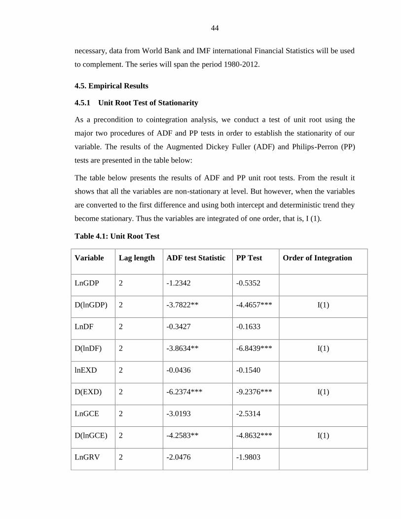
44
necessary, data from World Bank and IMF international Financial Statistics will be used
to complement. The series will span the period 1980-2012.
4.5. Empirical Results
4.5.1 Unit Root Test of Stationarity
As a precondition to cointegration analysis, we conduct a test of unit root using the
major two procedures of ADF and PP tests in order to establish the stationarity of our
variable. The results of the Augmented Dickey Fuller (ADF) and Philips-Perron (PP)
tests are presented in the table below:
The table below presents the results of ADF and PP unit root tests. From the result it
shows that all the variables are non-stationary at level. But however, when the variables
are converted to the first difference and using both intercept and deterministic trend they
become stationary. Thus the variables are integrated of one order, that is, I (1).
Table 4.1: Unit Root Test
Variable Lag length ADF test Statistic PP Test Order of Integration
LnGDP 2 -1.2342 -0.5352
D(lnGDP) 2 -3.7822** -4.4657*** I(1)
LnDF 2 -0.3427 -0.1633
D(lnDF) 2 -3.8634** -6.8439*** I(1)
lnEXD 2 -0.0436 -0.1540
D(EXD) 2 -6.2374*** -9.2376*** I(1)
LnGCE 2 -3.0193 -2.5314
D(lnGCE) 2 -4.2583** -4.8632*** I(1)
LnGRV 2 -2.0476 -1.9803

45
D(lnGRV) 2 -3.6750** -4.5812*** I(1)
Critical Values
1% -4.3139 -4.3139 -
5% -3.5742 -3.3742 -
10% -3.2226 -3.2224 -
*** represents stationary at 1% level of significance; ** represents stationary at 5%
level of significance; * represents stationary at 10% level of significance
Level represents Logarithms of variables; ‘D’ represents that the variable has been
differenced.
4.5.2 Johansen Cointegration Test
The result of Johansen cointegration test based on trace test is depicted in Table 4.2a.
The test based on trace statistics test the null hypothesis that there is no cointegration
among the variables. We reject the null hypothesis if the test statistic is greater than the
critical values of the trace tests at 1% or 5%.
Table 4.2b provides the results of Johansen cointegration test based on the maximum
eigenvalue. The test (maximum eigenvalue) is conducted on the null hypothesis of the
number of cointegrating equations (r) against the alternative hypothesis of number of
cointegrating equations plus one (r + 1). The null hypothesis cannot be rejected if the
test statistic is smaller than the maximum eigenvalue test critical value.
In table 4.2a, the trace test which is much stricter reflected that at least three
cointegrating equations exist at 5 per cent level of significance. As such the null
hypothesis of no cointegration will be rejected if the trace (test) statistic of 272.8, 160.6
and 88.8 is greater than the 5 per cent critical value of approximately 142.9, 90.7 and
73.8 respectively. Hence the trace statistics specified 3 cointegrating relationship at 5 per
cent levels of significance.
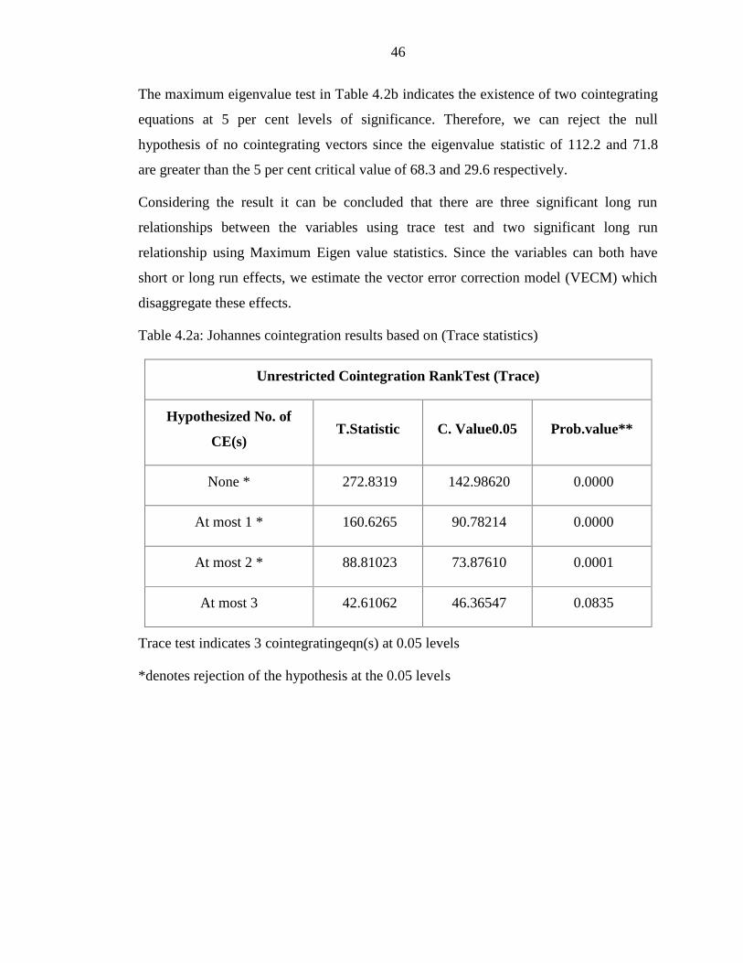
46
The maximum eigenvalue test in Table 4.2b indicates the existence of two cointegrating
equations at 5 per cent levels of significance. Therefore, we can reject the null
hypothesis of no cointegrating vectors since the eigenvalue statistic of 112.2 and 71.8
are greater than the 5 per cent critical value of 68.3 and 29.6 respectively.
Considering the result it can be concluded that there are three significant long run
relationships between the variables using trace test and two significant long run
relationship using Maximum Eigen value statistics. Since the variables can both have
short or long run effects, we estimate the vector error correction model (VECM) which
disaggregate these effects.
Table 4.2a: Johannes cointegration results based on (Trace statistics)
Unrestricted Cointegration RankTest (Trace)
Hypothesized No. of
CE(s)T.Statistic C. Value0.05 Prob.value**
None * 272.8319 142.98620 0.0000
At most 1 * 160.6265 90.78214 0.0000
At most 2 * 88.81023 73.87610 0.0001
At most 3 42.61062 46.36547 0.0835
Trace test indicates 3 cointegratingeqn(s) at 0.05 levels
*denotes rejection of the hypothesis at the 0.05 levels
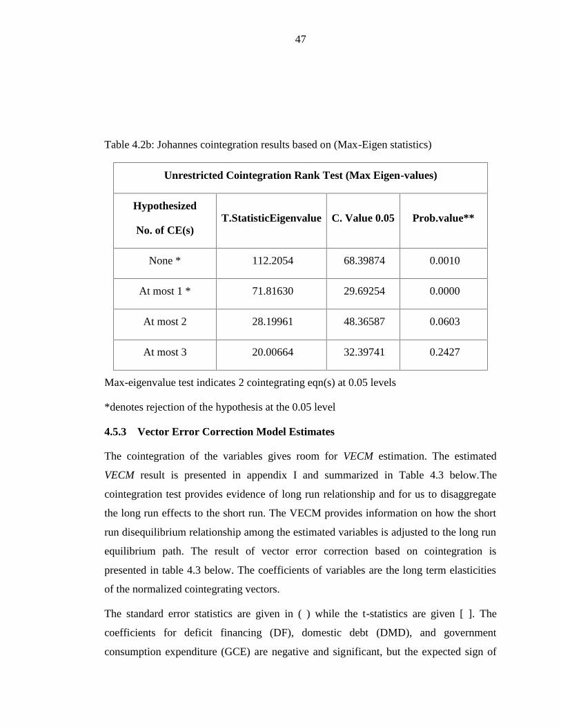
47
Table 4.2b: Johannes cointegration results based on (Max-Eigen statistics)
Unrestricted Cointegration Rank Test (Max Eigen-values)
Hypothesized
No. of CE(s)T.StatisticEigenvalue C. Value 0.05 Prob.value**
None * 112.2054 68.39874 0.0010
At most 1 * 71.81630 29.69254 0.0000
At most 2 28.19961 48.36587 0.0603
At most 3 20.00664 32.39741 0.2427
Max-eigenvalue test indicates 2 cointegrating eqn(s) at 0.05 levels
*denotes rejection of the hypothesis at the 0.05 level
4.5.3 Vector Error Correction Model Estimates
The cointegration of the variables gives room for VECM estimation. The estimated
VECM result is presented in appendix I and summarized in Table 4.3 below.The
cointegration test provides evidence of long run relationship and for us to disaggregate
the long run effects to the short run. The VECM provides information on how the short
run disequilibrium relationship among the estimated variables is adjusted to the long run
equilibrium path. The result of vector error correction based on cointegration is
presented in table 4.3 below. The coefficients of variables are the long term elasticities
of the normalized cointegrating vectors.
The standard error statistics are given in ( ) while the t-statistics are given [ ]. The
coefficients for deficit financing (DF), domestic debt (DMD), and government
consumption expenditure (GCE) are negative and significant, but the expected sign of
48
GCE were supposed to be positive it’s negative because of crowding out effects of
government expenditure to private investments.
On the other hand, the coefficients of external debt (EXD) and government revenue
(GRV) are positive and significant.
In Table 4.3 (Panel A), lnDF is negative and statistically significant at 5% level of
significance, as it relates to the level of gross domestic product. A 10% increase in
deficit financing will results in a decrease in gross domestic product by 0.9%. The result
for EXD is positive and significantly related to gross domestic product. A 10% increase
in external debt will results in an increase in gross domestic product by 0.8%. The result
for DMD is negatively and significantly related to GDP. A 10% increase in DMD will
results in a decrease in GDP by 1.9%. The result for GCE is negative and significantly
related to GDP. A 10% increase in GCE will results in a decrease in GDP by 1.1%. The
result for government revenue is positively and significantly related to GDP. A 10%
increase in GRV will results in an increase in GDP by 6.7%.
The speed of adjustment (dynamics of short run) is shown by the coefficient of the error
correction terms (ECM). The results are presented in Table 4.3 (Panel B). The
coefficient of D(lnGDP) is -0.398141. This indicates that, the speed of adjustment is
39.8% approximately. The implication is that, if there is a deviation from equilibrium
only 39.8% is corrected in one year as the variable moves towards restoring equilibrium.
Thus, there is relatively no strong pressure on lnGDP to restore long run equilibrium
wherever there is a disturbance. The speed of adjustment coefficient has the correct sign
(negative) and statistically significant with t-value of (-1.46).

49
Table 4.3: Results of Vector Error Correction Model
Panel A: Normalized Cointegrating Coefficients (Long Run Estimates)
lnGDP(-
1)
lnDF(-1) lnDMD(-
1)
lnEXD(-1) lnGCE(-1) lnGRV(-1) Constant
1.000000 -0.009565
(0.00294)
[-3.2536]
-0.192063
(0.03615)
[-5.3135]
0.083652
(0.01037)
[8.0702]
-0.112357
(0.03458)
[-3.2495]
0.675628
(0.03182)
[21.2302]
-1.465186
Panel B: Coefficients of Error Correction Terms
D(lnGDP) D(lnDF) D(lnEXD) D(lnDMD) D(lnGCE) D(lnGRV)
-0.398141
(0.27191)
[-1.46422]
-15.68030
(15.4445)
[-1.01526]
0.053027
(0.32830)
[0.16152]
1.971664
(0.91185)
[2.16227]
0.421998
(0.38826)
[1.08690]
2.186346
(0.45035)
[4.85481]
Source: Author’s computation as summary of appendix I (E-Views 7.0 iterations
Results);
Note: standard errors in ( ) and t-statistics in [ ]
4.5.4 Pairwise Granger Causality Test Analysis
Although the estimation of the Johansen cointegration established the existence of a
long-run equilibrium relationship among the variables of the VECM models, but this
does not provide any information about which of the variables cause the other. That is it
does not indicate the direction of causality among variables. It therefore (Granger
causality test) helps to determine the direction of causality between different variables of

50
the VEC model. The result of pairwise Granger causality test between gross domestic
product and instruments of fiscal policy can be presented in the table below:
.
The results in the table below indicate that a bi-directional causal relationship exists
between DMD to GDP; GRV to GDP and GRV to GCE. The result also provides
evidence for a uni-directional causal relationship running from GDP to GCE; GCE to
DF; EXD to DMD; EXD to GCE; and GCE to DMD.
Table 4.4: Pairwise Granger Causality Tests
Null Hypothesis: Obs F-Statistic Prob.
LNDMD does not Granger Cause LNGDP31
7.75739 0.0023
LNGDP does not Granger Cause LNDMD 5.37902 0.0111
LNGCE does not Granger Cause LNGDP31
0.14064 0.8695
LNGDP does not Granger Cause LNGCE 2.58915 0.0543
LNGRV does not Granger Cause LNGDP31
11.0523 0.0003
LNGDP does not Granger Cause LNGRV 11.2843 0.0003
LNGCE does not Granger Cause LNDF31
3.11928 0.0411
LNEXD does not Granger Cause LNDMD 2.87466 0.0545
LNGCE does not Granger Cause LNEXD31
0.48775 0.6195
LNEXD does not Granger Cause LNGCE 3.73711 0.0374
LNGRV does not Granger Cause LNEXD31
0.41789 0.6628
LNEXD does not Granger Cause LNGRV 1.39448 0.2659

51
LNGCE does not Granger Cause LNDMD31
8.71391 0.0013
LNDMD does not Granger Cause LNGCE 14.3404 0.0005
LNGRV does not Granger Cause LNDMD31
1.31753 0.2851
LNDMD does not Granger Cause LNGRV 14.7749 5.00E-05
LNGRV does not Granger Cause LNGCE31
3.18837 0.0478
LNGCE does not Granger Cause LNGRV 4.86886 0.016
Source: E-Views 7.0 iterations Test Results
4.5.5 Estimates for Impulse Responses
The response of GDP, DF, EXD, DMD, GCE and GRV to itself and to other variables in
the generalized ordering for the 9 years is presented and the analysis is based on three
periods of each term, where 1 to 3 periods represent the short term, 4 to 6 periods for
medium term and 7 to 9 periods for long term. Hence, the figures given at each of the
first periods are the basis of this analysis.
Table 4.51
Response of LOGGDP:
Period LOGGDP LOGDF LOGDM
DLOGEX
DLOGGR
VLOGGC
E
Short Term 685867.5 0.000000 0.000000 0.000000 0.000000 0.000000
MediumTerm 1941838. -455550 472842.9 324262.7 -291876.5 252088.8
Long Term 3397367. -2074265 1931315. 24021.96 -258084.4 475125.9
Source: E-Views 7.0 iterations Test Results
The response of LOGGDP to itself and other macroeconomic variables in table 4.5.1
above shows that, one unit shock of itself accounted for a positive response throughout
the periods. Also, a unit shock of LOGDMD and LOGGCE are positive throughout the
periods. But a unit shock of LOGDF and LOGGRV, are accounted for a negative
response of LOGGDP in the medium and long term but positive in the short term.

52
Response of LOGDF:
PeriodLOGGD
PLOGDF
LOGDM
DLOGEXD
LOGGR
V
LOGGC
E
Short Term 0.596874 4.224945 0.000000 0.0000000.00000
0
0.00000
0
Medium
Term-0.58241 1.628817 1.823122 -0.777107
0.95038
1
-
0.346546
Long Term -0.08185 0.252763 2.820783 -0.9156840.68015
1
0.02650
9
Source: extract from estimation output using E-views 7
The response of LOGDF to itself and other macroeconomic variables in table 4.5.2
Above shows that, one unit shock of itself accounted for a positive response throughout
the periods which is the same with LOGDMD and LOGVR. But a unit shock of
LOGGDP and LOGEXD accounted for a positive response in the short term but
negative in the medium and long term periods. Also, LOGGCE is accounted for a
negative response in the medium term but positive in the short and long term period.

53
Response of LOGDMD:
Period LOGGDP LOGDF LOGDMD LOGEXD LOGGRV LOGGCE
Short Term -23159-
40926.4142426.1 0.000000 0.000000 0.000000
Medium
Term198828.9 -219651 157850.9 13665.10 39498.22 -11292.5
Long Term 433903.7 -572613 526682.1 -123248.5 47651.30 48101.72
Source: extract from estimation output using E-views 7
The response of LOGDMD to itself and other macroeconomic variables in table 4.5.3
Above shows that, one unit shock of itself accounted for a positive response throughout
the periods which is the same with LOGGRV. But, LOGDF is negative throughout the
three periods. Also, a unit shock of LOGGDP is negative in the short term but positive
in the medium and long term periods. LOGEXD accounted for a positive response in
the short term and the medium but negative in long term period. Also, LOGGCE is
accounted for a negative response in the medium term but positive in the short and long
term period.

54
Response of LOGEXD:
PeriodLOGGD
PLOGDF
LOGDM
D
LOGEX
D
LOGGR
V
LOGGC
E
Short Term 104679.2 -108165 224053.8 197583.0 0.000000 0.000000
Medium
Term-761495 -240819 707245.3 186596.3 -500199 285876.9
Long Term -546054292112.
893815.21 340813.5 -436035.8 187769.2
Source: extract from estimation output using E-views 7
The response of LOGEXD to itself and other macroeconomic variables in table 4.5.4
Above shows that, one unit shock of itself accounted for a positive response throughout
the periods which is the same with LOGGCE and LOGDMD. But, LOGDF is negative
in the short and medium term but positive in the long term. Furthermore, a unit shock of
response in LOGGDP and LOGGRV are positive in the short term but negative in the
medium and long term periods.

55
Response of LOGGRV:
PeriodLOGGD
PLOGDF
LOGDM
D
LOGEX
D
LOGGR
V
LOGGC
E
Short Term 387478.372.5675
4-70727.8
-
146368.197264.98 0.000000
Medium
Term769568.6 -180073 42188.01 178734.7 -240424 192987.6
Long Term 889951.2 -294119 618577.2-
30288.61-422623.6 381135.7
Source: extract from estimation output using E-views 7
The response of LOGGRV to itself and other macroeconomic variables in table 4.5.5
Above shows that, one unit shock of itself accounted for a positive response in the short
term and a negative in the other periods which is the same with LOGDF. In addition,
LOGGDP and LOGGCE are positive throughout the three periods. LOGDMD is
negative in short but positive in medium and long term. But, LOGEXD is negative in the
short and long term but positive in the medium term.

56
Response of LOGGCE:
PeriodLOGGD
PLOGDF
LOGDM
D
LOGEX
D
LOGGR
V
LOGGC
E
Short Term -8836.66945.00
317695.47 6740.455 -24229.97 15431.48
Medium
Term15287.72
12002.4
614018.69 8359.236 -32978.58 22484.36
Long Term 27305.21 -2164.16 25213.74 1433.179 -21934.68 17284.40
Source: extract from estimation output using E-views 7
The response of LOGGCE to itself and other macroeconomic variables in table 4.5.6
Above shows that, one unit shock of itself accounted for a positive response throughout
the periods which is the same with LOGEXD and LOGDMD. But, LOGGDP is negative
in the short term and positive in the medium and long term. Furthermore, a unit shock of
response in LOGDF is positive in the short and medium term but, negative in the long
term periods.

57
CHAPTER FIVE
SUMMARY OF FINDINGS, CONCLUSION AND POLICY
RECOMMENDATIONS
5.1 Summary of Findings
This study investigates the impact of fiscal policy (using selected policy instruments as
proxies) on economic growth in Nigeria. The data used is time series and span 1980-
2012. The econometric technique used for the estimation of the model is Vector Error
Correction Model (VECM). The series were tested to determine their statistical
properties using Augmented Dickey Fuller (ADF) and Phillip Perron (PP). The series
were found to be stationary or integrated of order one, that is, I (1). Also, a cointegration
test was conducted. The result shows that, in Trace Test 3 cointegrating equation and 2
in Maximum Eigenvalue of the series used in the model.
The result of VECM shows that deficit financing, domestic debt and government
consumption expenditure are negative and significant determinants of gross domestic
product at 5% (α =0.05) level of significance. However, external debt and government
revenue are positive and statistically significant at 5% level of significance. The granger
causality test shows some variables having bi-directional causality, uni-directional
causality and others without any form of causality. The impulse response function shows
that the variables have various levels of shocks and innovation on itself and others.

58
5.2 Conclusion
In trying to achieve macroeconomic stability and sustainable growth in recent years,
there has been excessive reliance by the government at different levels (Federal, State
and local Government) on borrowing from different sources to finance fiscal deficits or
complement internal resources. Furthermore, It’s observed that, budget deficit is not the
critical issue of interest. Instead it’s the funding source, and quality of spending. The
problem of debt would of course result if those resources that should have been
deployed for the carrying out of productive programsare employed in the financing of
current or past consumption. It will bring about the need to evaluate the economic and
social rate of return of all government projects. Although some of the policy instruments
were found to be statistically insignificant, but the overall fiscal policy effect on the
Nigerian economic performance is significant looking at the result of Granger causality
and impulse response function.
5.3 Policy Recommendations
From the findings it’s observed that:
There is the need to address the problem of transparency on the part of the government.
Most of the government policies targets are deviated from the actual as a result of
secrecy in carrying out government programs and projects. Thereby, giving the policy
more credibility and public expectations may come closer to the objectives of the
government.
Conscious efforts must be made to improve the quality of government expenditure
especially in terms of contracts awards and execution. This is to ensure value for the use
of public resources.
Productive use of borrowed funds must be taking as a matter of necessity. Such funds
should be used in carrying out productive programs so that, the settlements of principal
and that of the interest elements will be improved. A powerful management of debt
demands that borrowed resources should not be unproductively utilized so that social
rate and that of the economic repay will be more than the future servicing cost of the
debt.

59
There is also the need to employed civil servants that are well grounded in policy
making. Most of the people in the field are not experts therefore cannot make policies
that will engender a great change.

60
BIBLIOGRAPHY
Abbas, S. and Christensen, J. (2007) the role of domestic debt market in economic growth:An Empirical Investigation for Low Income Countries and EmergingMarkets-IMF working Paper
Abubakar, M. (2008) ‘The Implication of Global Financial Crisis on InternationalMarketing’ Unpublished M.Sc. Assignment on International MarketingBayero University, Kano.
Adafu, S. N., Ogbolo F. and Essi D. (2010). Fiscal Policy and Economic Growth: Evidencefrom Nigeria (1970-2006). Journal of Economics, Management Studies andPolicy (JEMSAP), 3(1), 1 - 15.
Adam, C. S. and Bevan, D. L. (2004).Fiscal Deficits and Growth in Developing Countries.Journal of Public Economics, Vo.89, pp. 511-597.
Adefeso, G. and Mobolaji, W. (2010) Domestic debt and the Nigerian Economy, CurrentResearch Journal of Economic Theory 2(1):22-26
Adeoye, T. (2006) “Fiscal Policy and Growth of Nigerian Economy: An EmpiricalPerspective” NISER Monograph Series No 3, NISER Ibadan.
Adofu, I and Abula, M. (2010).Domestic debt and the Nigerian economy,Current ResearchJournal of Economic Theory 2(1):22-26
Ajayi, E.A. (1989). Nigerian debt management experience, Central Bank Nigeria, 13 (2)
Akanni K. A. and Osinowo O. H. (2013) “Effect of Fiscal Instability on Economic Growthin Nigeria”, Advances in Economics and Business 1(2): pp. 124-133.
Alison, J., (2003). Key issues for analyzing domestic debt sustainability. Debt ReliefInternational Publication, ISBN: 1-903971-07-1
Aniyanwu, J. E. and Oaikhenan, H. E. (1995).Modern Macroeconomics: Theory andApplications in Nigeria, Joanee Educational Publisher Ltd. pp363-386
Anyanwu, J.C. (1999) “An Analysis of the External Debt Burden of sub-Saharan Africa” inAfrica Debt Burden and Economic Development, NES days Conference inLagos.
Ashinze, R. and Onwioduokit, E. A. (2001), “Nigeria’s Economic Growth and ForeignDebt: An Analytical Re-Examination” CBN Economic and FinancialReview, 3(1), March.
61
Asogwa, R.C. (2005). Domestic government debt structure, risk characteristics andmonetary policy conduct, evidence from Nigeria. Access from:http://www.inf.org/external/np/res/seminars/2007/macro/pdf/asogwa.pdf
Bamidele, T. B. and Joseph, A. I. (2013), “Financial Crisis and External Debt Managementin Nigeria”, International Journal of Business and Behavioural Sciences3(4): pp. 62-
Barro, R. (1990). Government spending in a Simple model of Endogenous Growth.Journalof Political Economy, 98, S103 - S125.
Barro, R. and Sala-Martin, X. (1992).Public Finance in Models of Economic Growth.Review of Economic Studies, 59, 645 – 661
Barungi, B. and Michael, A. (2000) “Growth and Foreign Debt: The Ugandan Experience”in Ajai and Khan, External Debt and Capital Flight in sub-Saharan Africa,IMF.
Blinder, A. J. (2006) “The case against the case against discretionary fiscal policy”.In Themacroeconomics of fiscal policy. Cambridge: MIT Press.
Brauninger, M. (2002), “The Budget Deficit, Public Debt and Endogenous Growth”,Journal of Economics, 63(41): pp.1-15.
CBN, (2005) Statistical Bulleting, Central Bank Nigeria December, Vol. 16 Access from:http://www.cenbank.org/OUT/PUBLICATIONS/RE[PRTS/RD/207/STABULL-2005.PDF
Central Bank of Nigeria (2012) Annual Report and Statement of Accounts 31st Dec. 2012,Abuja.
Central Bank of Nigeria (2012) CBN Statistical Bulletin. CBN, Abuja.
Chamberlin, G. and Yueh, L. (2006).Macroeconomics.London: Thomsom Publishers.
Chenery, H. and Syrquim, M. (1975).Patterns of Development, 1950 - 1970. London:Oxford University Press.
Christensen, J., (2004), Domestic debt market in Sub-Saharan Africa. IMF Working PaperWp/0646.
Cohen, A. (2005) “Low Investment and Large LDC Debt in the 1980s” America EconomicReview, 34: pp. 199-208.
De Castro, F. (2004). The Macroeconomic Effects of Fiscal Policy in Spain”, Banco deEspana, Working Paper Series, http//www.bde.es
Diamond, J. (1990). Fiscal Indicators for Economic Growth: An Illusory Search. IMFWorking Paper, August.
Dickey, D. A. and Fuller, W. A. (1979). “Distribution of the Estimators for AutoregressiveTime Series with a Unit Root”, Journal of the American Statistical Association,74: pp. 427– 431.
Easterly, and Schmidt-Hebbel, K. (1993).Fiscal Adjustment and MacroeconomicPerformance. Outreach 10 May, (World Bank Policy Research Department).

62
Easterly, W. and Rebelo, S. (1994), ‘Fiscal Policy and Economic Growth: An EmpiricalInvestigation’, Journal of Monetary Economics, 32: 417-458.
Edwards, S. (2001) “Debt Relief and Fiscal Sustainability” NBER Working Paper 8939,Cambridge.
Ekpo, A. H. (1995). Public Expenditure and Economic Growth in Nigeria, 1960 - 1992.Fiscal Report, AERC, Nairobi, Kenya
Engel, R and Granger, C (1987) co-integration and error correction: representationestimation, testing, econometrics, 55:251-276
Engle, R. F., and Granger, C. W. J. (1987). Co-integration and Error Correction:Representation, Estimation, and Testing. Econometrica, 55, 251–276.
Eshang, E. (1983)An Expenditure Tax. Allen and Urwin, London.
Essien, E. A. andOnwioduokit, E. A. (2002) “Nigeria’s Economic Growth and ForeignDebt: An Analytical Re-Examination” CBN Economic and Financial Review,3(1), March.
Fatas, A. (2002) “The Effects of Business Cycles on Growth” Central Bank of ChileWorking Papers No 156.
Gemmel, N. (2001). Fiscal Policy in a Growth Framework.World Institute forDevelopment Economic Research, Discussion Paper No.2001/84, pp.1-23.
Granger, C. (1969).Developments in the Study of Cointegrated Economic Variables.Oxford Bulletin of Economics and Statistics, 48 (3), 355 - 369.
Gray, C. Tracey, L. and Varoudakis A. (2007): Fiscal Policy and Economic Growth.Lessons for Eastern Europe and Central Asia.World Bank; Washington, DC.
Grossman, H. and Elhannan, R. W. (1990) “Foreign Aid, Taxes and Public Investment”Journal of Development Economics, 24: pp. 355-369.
Grossman, P. J. (1997). Fiscal Decentralization and Public Sector Size in Austrialia.TheEconomic Record, 68(202), 240 – 246
Gunning, R. M. (1999)Economic Development. Allen and Urwin, London
Hnatkovska, V. and Loayza, N. (2005) “Volatility and Growth”, the World BankWorking Paper Series, No 3184.
Horton, M. and El-Ganainy, A. (2009) “What is Fiscal Policy?” Finance and Development.IMF’s Fiscal Affairs Department.
IMF (2001) Developing government bond markets: A Handbook (Washington).
Iyeli I. I. and Ijomah M. A. (2013), “A Re-examination of Fiscal Policy Applicability inNigeria’s Economic Growth Process: An Econometric Policy Evaluation fromEmpirical Evidence”, AMERICAN JOURNAL OF SOCIAL ISSUES ANDHUMANITIES, Vol. 3, Issues 4: pp. 180-
Iyoha, M. A. (1999) “External Debt and Economic Growth in sub-Saharan AfricanCountries: An Economic Study”, AERC Research Paper 90, Nairobi, Kenya.

63
Jhingan, M. L. (2003). Macroeconomic Theory.New Delhi: Vrinda Publishers.
Johansen, S. and Juselius, K. (1990).Maximum Likelihood Estimation and inference onCointegration, with Applications for the Demand for money.Oxford Bulletin ofEconomics and Statistics (52), 169 - 210.
Johansen, S., (1988).A Statistical Analysis of Co-integration Vectors.Journal of EconomicDynanmics& Control Vol. 12, pp. 231–254.
Kraay, A. and Vikram, N. (2004) “What is External Debt Sustainability”, World BankPolicy Research Working Paper 3200, February.
Lewis, W. A. (1955) the Theory of Economic Growth. Allen and Urwin, London.
Medee, P. N. and Nenbee, S. G. (2011), “Econometric Analysis of the Impact of FiscalPolicy Variables on Nigerian’s Economic Growth”, (1970 - 2009)”,International Journal of Economic Development Research and Investment,2(1): pp. 171-186.
Mihaljek, D.Scatigna, M. and Villar, A. (2002). Resent trend in bond markets BIS WorkingPaper 11,13-41
Mjema, G. D. (1996) “The Impact of Foreign Debt and Servicing in the Economic ofTanzania” African Journal of Economic Policy, 3(1).
Mohammed, S. T. (2009) “Domestic Debt Dynamics and Fiscal Sustainability in Nigeria:An Empirical Evidence” MPRA Paper No.18452, November.http://mpra.ub.uni- muenchen.de/18452/
Munongo, S. (2012), “Effectiveness of Fiscal Policy in Economic Growth: The Case ofZimbabwe”, International Journal of Economic Review 3(6): pp. 93 - 99
Musgrave, R. A and Musgrave P. B. (2005).Public Finance in Theory and Practice.(5thed.) New Delhi: Tata McGraw Hill publishing company.
Nathan, P. A. (2012), “The Impact of Fiscal Policy on the Nigerian Economy”,International Review of Social Sciences and Humanities 4(1): pp. 142-150.
Ndekwu, E. C. (1996) “Government Borrowing, Money Supply and Monetary Policy inNigeria”, NISER, Ibadan.
Newey, W. and K. West (1994).Automatic Lag Selection in Covariance Matrix Estimation.Review of Economic Studies, Vol. 61, pp. 631-653.
Nurske, R. (1953)Problems of Capital Formation in Underdeveloped Countries.OxfordUniversity Press.
Nwankwo, A. (2011). Federal government plans N794billion local debt to finance 2012deficit, The Nation News Paper of 17th Dec. 2011.
Obadan, M. I. (1988) “External Loans and National Development: The NigerianExperience” New Nigerian Bank Economic and Business Review, 1(2).
Obadan, M. I. and Uga, E. O. (2004) “Public Policies for Economic Development in aDeregulated Economy”, NCEMA Policy Analysis Series, 1.

64
Obiyeluaku, M. (2006) Fiscal Policy in Nigeria; fixed or Variable?University of KwaZulu-Natal.
Odozi, V.A (1996), Nigeria’s domestic public debt stock, an assessment CBN Debt Trend.20(2)
Oke, M. O. (2012) External Debt, Economic Growth and Investment in Nigeria: EuropeanJournal of Business and Management Vol. 4, No. 11
Okonjo-Iweala N. and Osafo K. P. (2007) ‘Nigeria’s Economic Reforms: Progress andChallenges’, The Brooking Institution, Washington, DC.www.brookings.edu/global
Okonjo-Iweala, (2011) “Frets over rising domestic liabilities”, The Nation News Paper of25th August, 2011.
Olukole, R(1991) Management of external debt of Nigeria, CBN Bullion,Vol.15, No 2
Omitogun, O. and Ayinla, T.A (2007) “Fiscal Policy and Nigeria Economic Growth”.Journal of research in national development volume 5 no 2, December 2007.
Oyejide T.A., Soyede A. and M.O. Kayode (2004): Nigeria and the IMF. HeinemannEducational book Nig. Ltd Ibadan.
Pattillo, C. A., Poirson, H., and Ricci, L. A. (2002).External debt and growth (IMFWorking Papers No. 02/69).International Monetary Fund.
Perotti R (2004). Estimating the effects of fiscal policy in OECD Countries.IGIER-University Bocconi and Centre for Economic Policy pp 1-43.
Philips, A. O (1997) “Nigerian Fiscal Policy, 1998 –2010”, Nigerian Institute of SocialEconomic Research (NISER), Monograph Series No. 17, Ibadan.
Phillips, P.C.B. and Perron, P. (1988)..Testing for a Unit Root in Time Series Regression.Biometrika, Vol.75, pp.335–346.
Rapu , S (2003) Assessment of Nigerian domestic debt sustainability- CBN Economic andFinancial Review, Vol 42 No2, 41-66.
Richard, W. K., Geoffrey, M. B. and Robert, K. T. (2009); “The Macroeconomics of FiscalPolicy”, Cambridge: MIT Press.
Salawu, A. (2004),“The Budget Deficit and Economic Performance: A Survey”,University of Wollongong, Economic Working Paper Series.
Sanusi, J (1988), Genesis of Nigerian debt problems and prospect of debt conversion; ALecture delivered on Debt Conversion/ Asset Trading organized byContinental Merchant Bank of Nigeria Limited.
Sowa, N.K. (1994) Fiscal Deficit, Output Growth and Inflation Target in Ghana”, WorldDevelopment 22(8).
Vincent N. E., Ioraver N. T. and Ezi-Herbert W. (2012) “Economic Growth and FiscalDeficits: Empirical Evidence from Nigeria”, Economics and FinanceReview 2(6): pp. 85 – 96.

65
World Bank, (2003) “Nigeria Policy Options for Growth and Stability”, Report No. 26215-NGA, Washington DC: The World Bank.
Wosowei E. (2013), “Fiscal Deficits and Macroeconomic Aggregates in Nigeria”, KuwaitChapter of Arabian Journal of Business and Management Review Vol. 2, No.9;May, 2013 : pp. 72-
Zaglar, M. &Durnker, G. (2003) “Fiscal policy and economic growth” Journal ofEconomic Surveys, 17(3.)
Zhattau, V. S. (2013) “Fiscal Policy as an Engine of Economic Growth in Nigeria”,International Journal of Arts and Humanities (African Researches Review) 2(2): pp. 282-298.

66
APPENDIX I: VECTOR ERROR CORRECTION MODELESTIMATION
LGDP = LNDF, LNEXD LNDMD, LNGCE LNGRV
Vector Error Correction Estimates
Date: 11/15/14 Time: 09:26
Sample (adjusted): 1983 2012
Included observations: 30 after adjustments
Standard errors in ( ) & t-statistics in [ ]
Cointegrating Eq: CointEq1
LNGDP(-1) 1.000000
LNDF(-1) -0.009565
(0.00294)
[-3.25361]
LNDMD(-1) -0.192063
(0.03615)
[-5.31353]
LNEXD(-1) 0.083652
(0.01037)
[ 8.07022]

67
LNGCE(-1) -0.112377
(0.03458)
[-3.24951]
LNGRV(-1) 0.675628
(0.03182)
[21.2302]
C -1.465186
Error Correction: D(LNGDP) D(LNDF) D(LNDMD) D(LNEXD) D(LNGCE) D(LNGRV)
CointEq1 -0.398141 -15.68030 0.053027 1.971664 0.421998 2.186346
(0.27191) (15.4445) (0.32830) (0.91185) (0.38826) (0.45035)
[ -1.46422] [-1.01526] [ 0.16152] [ 2.16227] [ 1.08690] [ 4.85481]
D(LNGDP(-1)) 0.134823 9.767444 0.335661 -1.369727 -0.058227 -0.490631
(0.36409) (20.6799) (0.43959) (1.22095) (0.51987) (0.60300)
[ 0.37030] [ 0.47232] [ 0.76358] [-1.12186] [-0.11200] [-0.81365]
D(LNGDP(-2)) -0.619723 4.791764 0.455930 -0.749295 0.687783 -1.375880
(0.31871) (18.1024) (0.38480) (1.06877) (0.45507) (0.52785)
[-1.94449] [ 0.26470] [ 1.18486] [-0.70108] [ 1.51137] [-2.60659]
D(LNDF(-1)) 0.007109 -0.220442 -0.013363 0.006697 -0.004777 0.024516
(0.00599) (0.34027) (0.00723) (0.02009) (0.00855) (0.00992)
[ 1.18675] [-0.64785] [-1.84751] [ 0.33338] [-0.55842] [ 2.47093]
D(LNDF(-2)) -0.001216 -0.136558 -0.014664 0.004264 -0.009613 0.001759
(0.00420) (0.23868) (0.00507) (0.01409) (0.00600) (0.00696)
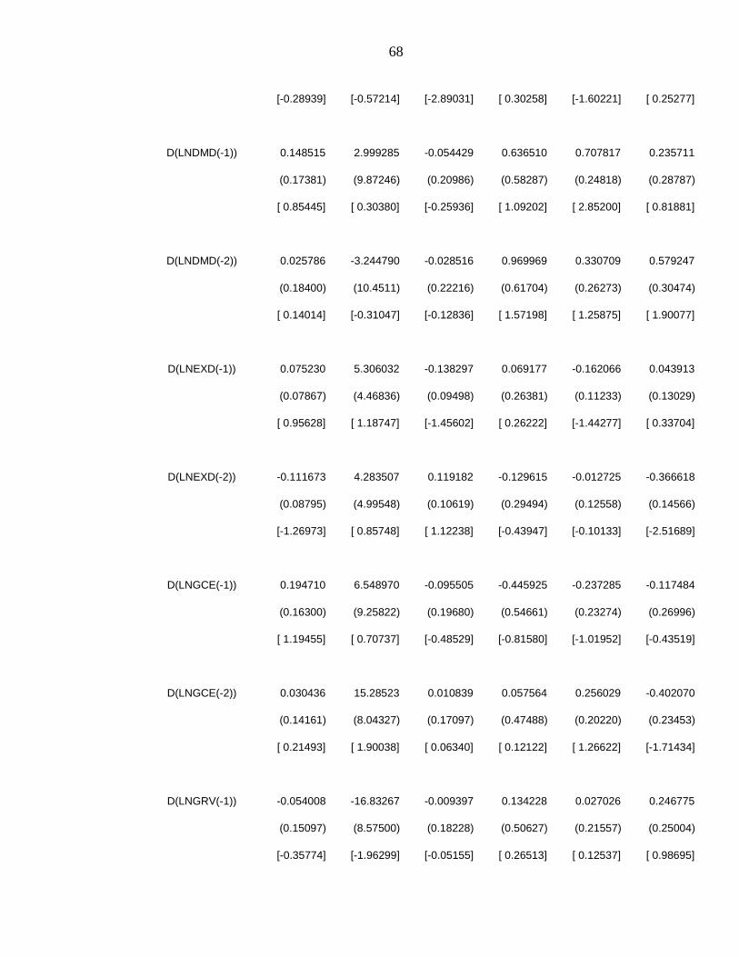
68
[-0.28939] [-0.57214] [-2.89031] [ 0.30258] [-1.60221] [ 0.25277]
D(LNDMD(-1)) 0.148515 2.999285 -0.054429 0.636510 0.707817 0.235711
(0.17381) (9.87246) (0.20986) (0.58287) (0.24818) (0.28787)
[ 0.85445] [ 0.30380] [-0.25936] [ 1.09202] [ 2.85200] [ 0.81881]
D(LNDMD(-2)) 0.025786 -3.244790 -0.028516 0.969969 0.330709 0.579247
(0.18400) (10.4511) (0.22216) (0.61704) (0.26273) (0.30474)
[ 0.14014] [-0.31047] [-0.12836] [ 1.57198] [ 1.25875] [ 1.90077]
D(LNEXD(-1)) 0.075230 5.306032 -0.138297 0.069177 -0.162066 0.043913
(0.07867) (4.46836) (0.09498) (0.26381) (0.11233) (0.13029)
[ 0.95628] [ 1.18747] [-1.45602] [ 0.26222] [-1.44277] [ 0.33704]
D(LNEXD(-2)) -0.111673 4.283507 0.119182 -0.129615 -0.012725 -0.366618
(0.08795) (4.99548) (0.10619) (0.29494) (0.12558) (0.14566)
[-1.26973] [ 0.85748] [ 1.12238] [-0.43947] [-0.10133] [-2.51689]
D(LNGCE(-1)) 0.194710 6.548970 -0.095505 -0.445925 -0.237285 -0.117484
(0.16300) (9.25822) (0.19680) (0.54661) (0.23274) (0.26996)
[ 1.19455] [ 0.70737] [-0.48529] [-0.81580] [-1.01952] [-0.43519]
D(LNGCE(-2)) 0.030436 15.28523 0.010839 0.057564 0.256029 -0.402070
(0.14161) (8.04327) (0.17097) (0.47488) (0.20220) (0.23453)
[ 0.21493] [ 1.90038] [ 0.06340] [ 0.12122] [ 1.26622] [-1.71434]
D(LNGRV(-1)) -0.054008 -16.83267 -0.009397 0.134228 0.027026 0.246775
(0.15097) (8.57500) (0.18228) (0.50627) (0.21557) (0.25004)
[-0.35774] [-1.96299] [-0.05155] [ 0.26513] [ 0.12537] [ 0.98695]
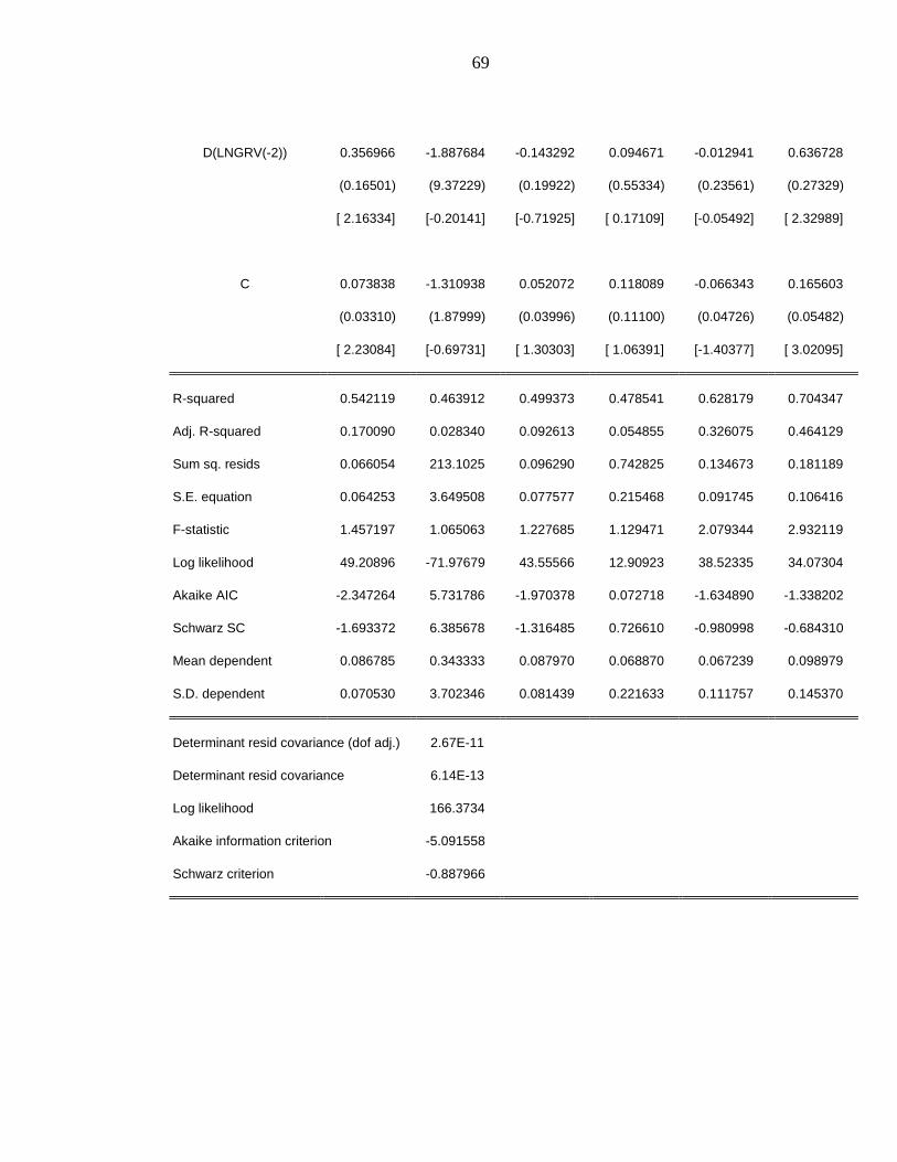
69
D(LNGRV(-2)) 0.356966 -1.887684 -0.143292 0.094671 -0.012941 0.636728
(0.16501) (9.37229) (0.19922) (0.55334) (0.23561) (0.27329)
[ 2.16334] [-0.20141] [-0.71925] [ 0.17109] [-0.05492] [ 2.32989]
C 0.073838 -1.310938 0.052072 0.118089 -0.066343 0.165603
(0.03310) (1.87999) (0.03996) (0.11100) (0.04726) (0.05482)
[ 2.23084] [-0.69731] [ 1.30303] [ 1.06391] [-1.40377] [ 3.02095]
R-squared 0.542119 0.463912 0.499373 0.478541 0.628179 0.704347
Adj. R-squared 0.170090 0.028340 0.092613 0.054855 0.326075 0.464129
Sum sq. resids 0.066054 213.1025 0.096290 0.742825 0.134673 0.181189
S.E. equation 0.064253 3.649508 0.077577 0.215468 0.091745 0.106416
F-statistic 1.457197 1.065063 1.227685 1.129471 2.079344 2.932119
Log likelihood 49.20896 -71.97679 43.55566 12.90923 38.52335 34.07304
Akaike AIC -2.347264 5.731786 -1.970378 0.072718 -1.634890 -1.338202
Schwarz SC -1.693372 6.385678 -1.316485 0.726610 -0.980998 -0.684310
Mean dependent 0.086785 0.343333 0.087970 0.068870 0.067239 0.098979
S.D. dependent 0.070530 3.702346 0.081439 0.221633 0.111757 0.145370
Determinant resid covariance (dof adj.) 2.67E-11
Determinant resid covariance 6.14E-13
Log likelihood 166.3734
Akaike information criterion -5.091558
Schwarz criterion -0.887966

70
APPENDIX II: IMPULSE RESPONSE (Figure)
Response of
LOGGDP:
Period LOGGDP LOGDF LOGDMD LOGEXD LOGGRV LOGGCE
1 685867.5 0.000000 0.000000 0.000000 0.000000 0.0000002 1146656. -22407.86 490017.3 176611.5 -374210.1 280725.13 1711082. -389289.6 141597.4 160200.9 -63992.13 97416.304 1941838. -455550.4 472842.9 324262.7 -291876.5 252088.85 2170160. -1030653. 962821.2 222497.7 130446.6 -8660.0676 2614934. -1541188. 1592688. -59430.70 -207712.5 346743.77 3397367. -2074265. 1931315. 24021.96 -258084.4 475125.98 3987775. -2903990. 2053797. 121273.3 319312.6 59712.699 4385355. -3731786. 3210575. -28488.32 148528.2 289740.3
Response of
LOGDF:
Period LOGGDP LOGDF LOGDMD LOGEXD LOGGRV LOGGCE
1 0.596874 4.224945 0.000000 0.000000 0.000000 0.0000002 0.963461 3.300207 1.054401 -0.099660 -0.014579 0.2115233 -0.209701 2.570294 1.268056 -0.564768 0.396273 0.0531934 -0.582406 1.628817 1.823122 -0.777107 0.950381 -0.3465465 -0.907491 1.027903 3.113749 -0.968769 0.500492 0.0249136 -0.358026 0.451728 2.858029 -1.239113 0.418171 0.2464897 -0.081846 0.252763 2.820783 -0.915684 0.680151 0.0265098 -0.096247 -0.803935 3.813540 -1.158922 1.646342 -0.6373059 0.448591 -1.831276 5.482024 -2.027388 0.927876 0.210528
Response ofLOGDMD:
Period LOGGDP LOGDF LOGDMD LOGEXD LOGGRV LOGGCE
1 -23159.02 -40926.42 142426.1 0.000000 0.000000 0.0000002 26599.54 -134122.7 204068.5 -59531.38 -5519.605 20349.503 134129.0 -148698.7 211431.8 -40232.99 -93166.81 94772.094 198828.9 -219650.9 157850.9 13665.10 39498.22 -11292.505 186343.7 -307079.7 297585.7 -20303.34 46131.01 -11406.736 259572.1 -412570.4 489173.4 -101581.7 -16916.59 74080.007 433903.7 -572613.1 526682.1 -123248.5 47651.30 48101.72
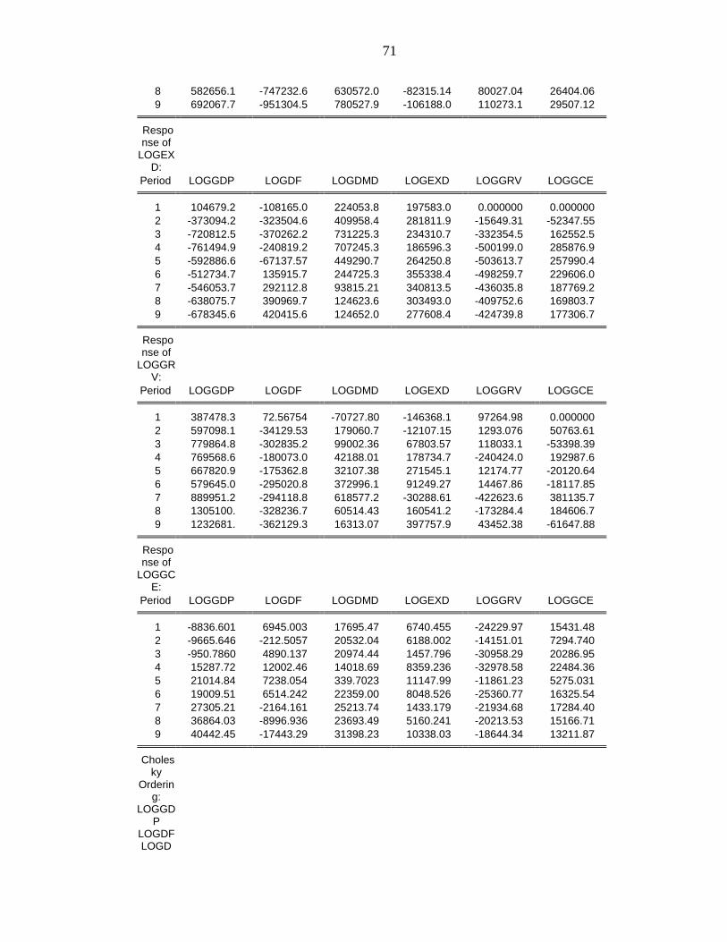
71
8 582656.1 -747232.6 630572.0 -82315.14 80027.04 26404.069 692067.7 -951304.5 780527.9 -106188.0 110273.1 29507.12
Response of
LOGEXD:
Period LOGGDP LOGDF LOGDMD LOGEXD LOGGRV LOGGCE
1 104679.2 -108165.0 224053.8 197583.0 0.000000 0.0000002 -373094.2 -323504.6 409958.4 281811.9 -15649.31 -52347.553 -720812.5 -370262.2 731225.3 234310.7 -332354.5 162552.54 -761494.9 -240819.2 707245.3 186596.3 -500199.0 285876.95 -592886.6 -67137.57 449290.7 264250.8 -503613.7 257990.46 -512734.7 135915.7 244725.3 355338.4 -498259.7 229606.07 -546053.7 292112.8 93815.21 340813.5 -436035.8 187769.28 -638075.7 390969.7 124623.6 303493.0 -409752.6 169803.79 -678345.6 420415.6 124652.0 277608.4 -424739.8 177306.7
Response of
LOGGRV:
Period LOGGDP LOGDF LOGDMD LOGEXD LOGGRV LOGGCE
1 387478.3 72.56754 -70727.80 -146368.1 97264.98 0.0000002 597098.1 -34129.53 179060.7 -12107.15 1293.076 50763.613 779864.8 -302835.2 99002.36 67803.57 118033.1 -53398.394 769568.6 -180073.0 42188.01 178734.7 -240424.0 192987.65 667820.9 -175362.8 32107.38 271545.1 12174.77 -20120.646 579645.0 -295020.8 372996.1 91249.27 14467.86 -18117.857 889951.2 -294118.8 618577.2 -30288.61 -422623.6 381135.78 1305100. -328236.7 60514.43 160541.2 -173284.4 184606.79 1232681. -362129.3 16313.07 397757.9 43452.38 -61647.88
Response of
LOGGCE:
Period LOGGDP LOGDF LOGDMD LOGEXD LOGGRV LOGGCE
1 -8836.601 6945.003 17695.47 6740.455 -24229.97 15431.482 -9665.646 -212.5057 20532.04 6188.002 -14151.01 7294.7403 -950.7860 4890.137 20974.44 1457.796 -30958.29 20286.954 15287.72 12002.46 14018.69 8359.236 -32978.58 22484.365 21014.84 7238.054 339.7023 11147.99 -11861.23 5275.0316 19009.51 6514.242 22359.00 8048.526 -25360.77 16325.547 27305.21 -2164.161 25213.74 1433.179 -21934.68 17284.408 36864.03 -8996.936 23693.49 5160.241 -20213.53 15166.719 40442.45 -17443.29 31398.23 10338.03 -18644.34 13211.87
Cholesky
Ordering:
LOGGDP
LOGDFLOGD

72
MDLOGEX
DLOGGR
VLOGGC
E

73
APPENDIX III: GRANGER CAUSALITY
Pairwise Granger Causality Tests
Date: 11/13/14 Time: 14:12
Sample: 1980 2012
Lags: 2
Null Hypothesis: Obs F-Statistic Prob.
LNDF does not Granger Cause LNGDP 31 1.40974 0.2623
LNGDP does not Granger Cause LNDF 1.56428 0.2283
LNEXD does not Granger Cause LNGDP 31 1.33466 0.2807
LNGDP does not Granger Cause LNEXD 0.06000 0.9419
LNDMD does not Granger Cause LNGDP 31 7.75739 0.0023
LNGDP does not Granger Cause LNDMD 5.37902 0.0111
LNGCE does not Granger Cause LNGDP 31 0.14064 0.8695
LNGDP does not Granger Cause LNGCE 2.58915 0.0543
LNGRV does not Granger Cause LNGDP 31 11.0523 0.0003
LNGDP does not Granger Cause LNGRV 11.2843 0.0003
LNEXD does not Granger Cause LNDF 31 1.22694 0.3096
LNDF does not Granger Cause LNEXD 0.47273 0.6286

74
LNDMD does not Granger Cause LNDF 31 1.76778 0.1906
LNDF does not Granger Cause LNDMD 0.11576 0.8911
LNGCE does not Granger Cause LNDF 31 3.11928 0.0411
LNDF does not Granger Cause LNGCE 0.08078 0.9226
LNGRV does not Granger Cause LNDF 31 1.54923 0.2314
LNDF does not Granger Cause LNGRV 1.01005 0.3780
LNDMD does not Granger Cause LNEXD 31 0.39479 0.6778
LNEXD does not Granger Cause LNDMD 2.87466 0.0545
LNGCE does not Granger Cause LNEXD 31 0.48775 0.6195
LNEXD does not Granger Cause LNGCE 3.73711 0.0374
LNGRV does not Granger Cause LNEXD 31 0.41789 0.6628
LNEXD does not Granger Cause LNGRV 1.39448 0.2659
LNGCE does not Granger Cause LNDMD 31 8.71391 0.0013
LNDMD does not Granger Cause LNGCE 14.3404 6.E-05
LNGRV does not Granger Cause LNDMD 31 1.31753 0.2851
LNDMD does not Granger Cause LNGRV 14.7749 5.E-05
LNGRV does not Granger Cause LNGCE 31 3.18837 0.0478
LNGCE does not Granger Cause LNGRV 4.86886 0.0160
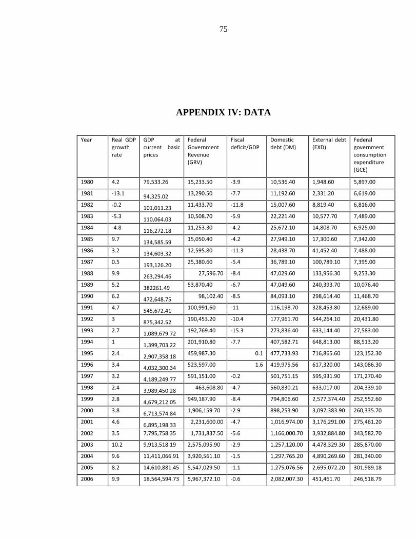
75
APPENDIX IV: DATA
Year Real GDPgrowthrate
GDP atcurrent basicprices
FederalGovernmentRevenue(GRV)
Fiscaldeficit/GDP
Domesticdebt (DM)
External debt(EXD)
Federalgovernmentconsumptionexpenditure(GCE)
1980 4.2 79,533.26 15,233.50 -3.9 10,536.40 1,948.60 5,897.00
1981 -13.1 94,325.02 13,290.50 -7.7 11,192.60 2,331.20 6,619.00
1982 -0.2 101,011.23 11,433.70 -11.8 15,007.60 8,819.40 6,816.00
1983 -5.3 110,064.03 10,508.70 -5.9 22,221.40 10,577.70 7,489.00
1984 -4.8 116,272.18 11,253.30 -4.2 25,672.10 14,808.70 6,925.00
1985 9.7 134,585.59 15,050.40 -4.2 27,949.10 17,300.60 7,342.00
1986 3.2 134,603.32 12,595.80 -11.3 28,438.70 41,452.40 7,488.00
1987 0.5 193,126.20 25,380.60 -5.4 36,789.10 100,789.10 7,395.00
1988 9.9 263,294.46 27,596.70 -8.4 47,029.60 133,956.30 9,253.30
1989 5.2 382261.49 53,870.40 -6.7 47,049.60 240,393.70 10,076.40
1990 6.2 472,648.75 98,102.40 -8.5 84,093.10 298,614.40 11,468.70
1991 4.7 545,672.41 100,991.60 -11 116,198.70 328,453.80 12,689.00
1992 3 875,342.52 190,453.20 -10.4 177,961.70 544,264.10 20,431.80
1993 2.7 1,089,679.72 192,769.40 -15.3 273,836.40 633,144.40 27,583.00
1994 1 1,399,703.22 201,910.80 -7.7 407,582.71 648,813.00 88,513.20
1995 2.4 2,907,358.18 459,987.30 0.1 477,733.93 716,865.60 123,152.30
1996 3.4 4,032,300.34 523,597.00 1.6 419,975.56 617,320.00 143,086.30
1997 3.2 4,189,249.77 591,151.00 -0.2 501,751.15 595,931.90 171,270.40
1998 2.4 3,989,450.28 463,608.80 -4.7 560,830.21 633,017.00 204,339.10
1999 2.8 4,679,212.05 949,187.90 -8.4 794,806.60 2,577,374.40 252,552.60
2000 3.8 6,713,574.84 1,906,159.70 -2.9 898,253.90 3,097,383.90 260,335.70
2001 4.6 6,895,198.33 2,231,600.00 -4.7 1,016,974.00 3,176,291.00 275,461.20
2002 3.5 7,795,758.35 1,731,837.50 -5.6 1,166,000.70 3,932,884.80 343,582.70
2003 10.2 9,913,518.19 2,575,095.90 -2.9 1,257,120.00 4,478,329.30 285,870.00
2004 9.6 11,411,066.91 3,920,561.10 -1.5 1,297,765.20 4,890,269.60 281,340.00
2005 8.2 14,610,881.45 5,547,029.50 -1.1 1,275,076.56 2,695,072.20 301,989.18
2006 9.9 18,564,594.73 5,967,372.10 -0.6 2,082,007.30 451,461.70 246,518.79

76
2007 9.7 20,657,317.67 6,034,615.60 -2.3 2,941,813.48 431,079.85 460,539.99
2008 8.5 24,296,329.29 7,866,590.38 -5.7 2,320,310.00 523,254.09 453,716.95
2009 6.4 24,794,238.66 4,844,592.34 -3.4 3,228,030.00 590,437.13 445,086.51
2010 6.3 33,984,754.13 7,303,671.55 -0.3 4,551,820.00 689,837.49 587,664.67
2011 7.8 37,409,860.61 11,116,900.00 -1.3 5,622,800.00 896,849.62 654,437.09
2012 8.5 40,544,099.94 10,654,724.87 -1.5 6,537,536.31 1,026,903.92 709,090.81

77
APPENDIX V: FIGURE 3
Year Real GDP growth rate GRV % GDP1980 4.2 01981 -13.1 -12.754783861982 -0.2 -13.970881461983 -5.3 -8.0901195591984 -4.8 7.0855576811985 9.7 33.742102321986 3.2 -16.309201081987 0.5 101.50050021988 9.9 8.7314720691989 5.2 95.205948541990 6.2 82.108170721991 4.7 2.9450859511992 3 88.58320891993 2.7 1.216151791994 1 4.7421426841995 2.4 127.81708561996 3.4 13.828577441997 3.2 12.901907381998 2.4 -21.575232051999 2.8 104.73897392000 3.8 100.82005892001 4.6 17.073086792002 3.5 -22.394806422003 10.2 48.691542942004 9.6 52.249129832005 8.2 41.485602662006 9.9 7.5777963682007 9.7 1.1268528072008 8.5 30.357770922009 6.4 -38.415601862010 6.3 50.759259762011 7.8 52.209747162012 8.5 -4.157410159

78
APPENDIX VI: FIGURE 2
YearReal GDP growthrate
EXD % OFGDP DMD % GDP
1980 4.2 0 01981 -13.1 19.63460946 6.227933641982 -0.2 278.3201784 34.085020461983 -5.3 19.93673039 48.067645731984 -4.8 39.99924369 15.528724561985 9.7 16.82727046 8.8695509911986 3.2 139.6009387 1.751755871987 0.5 143.1441847 29.362804911988 9.9 32.90752671 27.835690461989 5.2 79.45680793 0.0425264091990 6.2 24.21889592 78.732869141991 4.7 9.992619244 38.178637721992 3 65.70491801 53.152918231993 2.7 16.33036241 53.873782951994 1 2.474727724 48.84168431995 2.4 10.4887849 17.2115299
1996 3.4 -13.88622916-
12.090070721997 3.2 -3.464669863 19.471511631998 2.4 6.223043271 11.774573911999 2.8 307.1572169 41.719648092000 3.8 20.17593951 13.015405262001 4.6 2.5475402 13.216764212002 3.5 23.82004042 14.653934122003 10.2 13.86881457 7.8146865612004 9.6 9.198526334 3.233199695
2005 8.2 -44.88908751-
1.7482854372006 9.9 -83.24862317 63.284885422007 9.7 -4.514635461 41.296982
2008 8.5 21.38217316-
21.126542672009 6.4 12.83946772 39.120634742010 6.3 16.83504559 41.009222342011 7.8 30.0088257 23.528610532012 8.5 14.50123823 16.26834157

79
APPENDIX VII: FIGURE 1
YearReal GDPgrowth rate Fiscal deficit/GDP
1980 4.2 -3.91981 -13.1 -7.71982 -0.2 -11.81983 -5.3 -5.91984 -4.8 -4.21985 9.7 -4.21986 3.2 -11.31987 0.5 -5.41988 9.9 -8.41989 5.2 -6.71990 6.2 -8.51991 4.7 -111992 3 -10.41993 2.7 -15.31994 1 -7.71995 2.4 0.11996 3.4 1.61997 3.2 -0.21998 2.4 -4.71999 2.8 -8.42000 3.8 -2.92001 4.6 -4.72002 3.5 -5.62003 10.2 -2.92004 9.6 -1.52005 8.2 -1.12006 9.9 -0.62007 9.7 -2.32008 8.5 -5.72009 6.4 -3.4

80
2010 6.3 -0.32011 7.8 -1.32012 8.5 -1.5


