Institute for Research on Poverty Discussion Paper no. 1305-05

The Impact of Family Income on Child Achievement

Gordon Dahl University of Rochester

and NBER

Lance Lochner University of Western Ontario

and NBER

August 2005

We thank Mark Bils, David Blau, David Dahl, Greg Duncan, Rick Hanushek, Shakeeb Khan, Uta Schoenberg, Todd Stinebrickner, Chris Taber, and Mo Xiao for helpful comments. We also thank seminar participants at Brigham Young University, the Federal Reserve Bank of Cleveland, the Institute for Research on Poverty Summer Workshop, the National Bureau of Economic Research Summer Meetings, Northwestern University, and the University of Toronto for their comments. Marina Renzo and Fernando Levia provided excellent research assistance. Both authors gratefully acknowledge financial support from the William T. Grant Foundation. Lochner also acknowledges support from the Social Sciences and Humanities Research Council of Canada. IRP Publications (discussion papers, special reports, and the newsletter Focus) are available on the Internet. The IRP Web site can be accessed at the following address: http://www.irp.wisc.edu

Abstract

Understanding the consequences of growing up poor for a child’s well-being is an important

research question, but one that is difficult to answer due to the potential endogeneity of family income.

Past estimates of the effect of family income on child development have often been plagued by omitted

variable bias and measurement error. In this paper, we use a fixed effect instrumental variables strategy to

estimate the causal effect of income on children’s math and reading achievement. Our primary source of

identification comes from the large, non-linear changes in the Earned Income Tax Credit (EITC) over the

last two decades. The largest of these changes increased family income by as much as 20 percent, or

approximately $2,100. Using a panel of over 6,000 children matched to their mothers from National

Longitudinal Survey of Youth datasets allows us to address problems associated with unobserved

heterogeneity and endogenous transitory income shocks as well as measurement error in income. Our

baseline estimates imply that a $1,000 increase in income raises math test scores by 2.1 percent and

reading test scores by 3.6 percent of a standard deviation. The results are even stronger when looking at

children from disadvantaged families who are affected most by the large changes in the EITC, and are

robust to a variety of alternative specifications.

1 Introduction

In 2003, 12.9 million children in the U.S. under the age of 18, or more than one in six children, were

living in poverty (U.S. Census Bureau, 2004). Given such a high poverty rate, the consequences

of growing up poor on child well-being and future success has emerged as an important research

topic. Of particular interest is whether income support programs like the Earned Income Tax

Credit (EITC) can improve child development. However, the extent to which income maintenance

programs, and family income more generally, impact children is not easily estimated.

The major challenge faced by researchers attempting to estimate the causal effect of family

income on children’s outcomes has been the endogeneity of income. In particular, children growing

up in poor families are likely to have adverse home environments or face other challenges which

would continue to affect their development even if family income were to increase substantially.

These concerns have prevented the literature from reaching a consensus on whether family income

has a casual effect on child development (e.g., see Duncan and Brooks-Gunn (1997), Haveman

and Wolfe (1995), Mayer (1997)).

Since the mid-1990’s, one of the largest federal anti-poverty programs in the U.S. has been the

EITC, which provides cash assistance to low-income families and individuals who have earnings

from work.1 Low income families with two or more children can receive a credit of up to 40% of

their income in recent years (up to $4,204 in 2003), while families with one child can receive a

credit of up to 34%. In 2003, the EITC provided $37.5 billion in income benefits to 20.8 million

families and individuals, lifting more children out of poverty than any other government program

(Center on Budget and Policy Priorities, 2005). It is natural to ask what effect the EITC and

other income maintenance programs have on disadvantaged children. In this paper, we analyze

the impact of changes in family income on child cognitive outcomes.

We use a fixed effect instrumental variables (FEIV) strategy to estimate the causal effect

of income on children’s achievement. Our approach accounts for both permanent unobserved

heterogeneity and temporary shocks to children’s outcomes which may be correlated with family

income. Permanent heterogeneity is dealt with using fixed effects methods, while transitory shocks

to the family are addressed using instrumental variables. We estimate the effect of changes in

after-tax/transfer family income (rather than pre-tax income) on changes in children’s outcomes.1See Hotz and Scholz (2003) for a more detailed description of the EITC program and a summary of related

research.

1

As our instrument for changes in after-tax/transfer income, we use predicted changes in after-

tax/transfer family income based on predetermined, exogenous family characteristics (such as

race and mother’s age) and changes in the federal EITC schedule.

To estimate our FEIV model, we use panel data on over 6,000 children matched to their

mothers in the Children of the National Longitudinal Survey of Youth (NLSY). These data

contain a rich set of income and demographic measures. More importantly, these data have up

to five repeated measures of cognitive test scores per child taken every other year, which allows

us to account for unobserved child fixed effects.

Our primary source of identification comes from the large changes in the EITC schedule that

took place throughout the 1980s and 1990s (see Figures 1 and 2). The largest increase began

in 1994, when sizeable expansions of the credit were phased in over a three-year period. From

1993 to 1997, the subsidy rate for low income families with two children rose from 19.5% to

40%, while the maximum allowable credit more than doubled, rising from $1,801 to $3,923 (in

year 2000 dollars). Since changes in the federal EITC schedule should not be correlated with

idiosyncratic shocks to families, predicted changes in EITC benefits (where the predictions are

based on exogenous characteristics of the mother) can serve as an exogenous source of changes

in family income.

A simple example helps illustrate our identification strategy. Consider using race as an ex-

ogenous predictor of family income. Since blacks have lower family income on average and the

EITC expansion in the mid-1990s targeted low income families, black families were more likely

to receive an exogenous boost to their family income over that period. If family income has a

positive causal effect on children, the increase in EITC income for black families relative to white

families should have improved the relative outcomes of black children. Based on this observation,

one could construct a simple Wald estimate of the effect of family income on child test scores.

That is, one could divide the change in the average difference in test scores between black and

white children before and after the EITC increase by the change in the average difference in

income. Our estimation strategy is analogous, although we use a vector of exogenous variables to

predict income changes and take advantage of changes in the EITC schedule over multiple years

to obtain more precise estimates.

We also consider a second novel source of identification, which exploits changes in the national

earnings structure over time, to identify exogenous changes in income that vary across families.

2

For example, consider the dramatic increase in the return to education over the last few decades.

This implies that family income has risen more, on average, for more educated families. As a

consequence, everything else equal, child test scores from families with more educated parents

should have improved relative to those from families with less educated parents. Our estimation

strategy also incorporates this insight using multiple years of data and other exogenous parental

characteristics to predict income changes.

Using our FEIV approach, we find that current income has a significant effect on a child’s math

and reading test scores. Our baseline estimates imply that a $1,000 increase in family income

would raise math test scores by 2.1% and reading test scores by 3.6% of a standard deviation.

The effects are substantially stronger for blacks and hispanics than for whites. When we account

for changes in maternal labor supply or consider alternative specifications, our main conclusions

are unaffected. All of our findings suggest that supplementing the income of poor parents can

significantly increase the scholastic achievement of children.

Our FEIV estimates, while modest, are larger than cross-section OLS or standard fixed effects

estimates. One explanation is that income is noisily measured, so that OLS and FE estimates

suffer from attenuation bias. It is also possible that income matters more for the most disad-

vantaged, and that our instrument is largely picking up the effect for these families. Perhaps

the most interesting explanation is that expectations about future income play an important role

in determining child outcomes. In this case, permanent changes in family income should have

larger effects on children than do temporary changes. To the extent that changes in the EITC

are expected to last longer than most other shocks to family income, our FEIV estimates should

be greater than traditional fixed effect estimates. Additionally, FEIV estimates should be greater

during periods when the EITC changed most and for families predicted to receive the largest

EITC increases. Our estimates are consistent with all of these predictions.

The remainder of this paper proceeds as follows. In the next section, we provide a brief

literature review. Section 3 discusses our strategy for estimating the effect of family income

on child outcomes. We then discuss our data and document the large changes in the EITC in

Section 4. Section 5 presents the baseline estimates of the effect of income on math and reading

test scores, and Section 6 presents robustness checks. We conclude in Section 7.

3

2 Previous Research

A growing empirical literature questions how poverty affects a child’s well-being and whether

income support programs can improve children’s life chances. However, evidence on the extent to

which family income affects child development is mixed. Previous studies differ in data, methods,

and findings, as discussed in the recent collection of studies in Brooks-Gunn and Duncan (1997)

or the surveys in Haveman and Wolfe (1995) and Mayer (1997).

Researchers have provided several explanations for why family income might affect child de-

velopment. First, poverty is associated with increased levels of parental stress, depression, and

poor health – conditions which might adversely affect parents’ ability to nurture their children.

For example, in 1998, 27% of kindergartners living in poverty had a parent at risk for depression,

compared to 14% for other kindergartners (Child Trends and Center for Child Health Research,

2004). Low income parents also report a higher level of frustration and aggravation with their

children, and these children are more likely to have poor verbal development and exhibit higher

levels of distractability and hostility in the classroom (Parker et. al, 1999). Extra family income

might also matter if parents use the money for child-centered goods like books, for quality daycare

or preschool programs, for better dependent health care, or to move to a better neighborhood.2

Until recently, empirical studies linking poverty and income to child outcomes have done

little to eliminate biases caused by the omission of unobserved family and child characteristics.

Most studies employ regressions of an outcome variable (such as scholastic achievement) on some

measure of family income and a set of observable family, child, and neighborhood characteristics.

While these studies reveal the correlations between income and child outcomes, they do not

necessarily estimate a causal relationship as Mayer (1997), Brooks-Gunn and Duncan (1997), and

others have pointed out. Children living in poor families may have a worse home environment or

other characteristics that the researcher does not observe. These omitted variables may be part of

the reason for substandard achievement and may continue to affect children’s development even

if family income were to rise.

Blau (1999), Duncan, et. al (1998), and Levy and Duncan (1999) use fixed effects estima-

tion strategies to eliminate biases caused by permanent family or child characteristics. All three2Low income parents have fewer children’s books in their homes and spend less time reading to their children,

markers which are negatively associated with future academic performance. Children in poor families are also lesslikely to receive adequate health care and nutrition, both of which might affect performance in school. Finally,neighborhood poverty has been associated with underfunded public schools and lower achievement scores amongyoung children (Child Trends and Center for Child Health Research, 2004).

4

studies use differences in family income levels across siblings to remove fixed family factors when

estimating the impacts of income on child outcomes. Using PSID data, both Duncan, et. al

(1998) and Levy and Duncan (1999) find that family income at early ages is more important for

determining educational attainment whether they control for fixed family effects or not. Using

data from the Children of the NLSY, Blau (1999) reaches somewhat different conclusions. When

controlling for “grandparent fixed effects” – comparing the children of sisters – he finds larger

impacts for “permanent income” than when running standard OLS regressions. On the other

hand, he finds smaller and insignificant effects of current family income on ability and behav-

ioral outcomes when he uses fixed effect strategies (regardless of whether he uses comparisons of

cousins, siblings, or repeated observations for the same individual). While these papers represent

a significant step forward, they do not control for endogenous transitory shocks and they may

suffer from severe attenuation bias, since growth rates in income are noisily measured.3

Another line of research uses data from welfare and anti-poverty experiments conducted during

the 1990s. Except for a recent working paper by Duncan, et. al (2004), these studies focus on

program impacts, but do not separate out the effects of family income from other aspects of the

programs. Duncan, et. al (2004) combine data from four of these experiments in an attempt to

separately estimate the effect of family income versus employment and welfare effects induced

by the programs. They find a relatively large effect of family income on school achievement for

preschool children but not older children.

The different conclusions reached by recent studies suggest that unobserved heterogeneity

may be an important issue. In the following section, we propose a new FEIV strategy which

eliminates omitted variable biases due to both permanent and temporary shocks correlated with

family income. Our approach also eliminates attenuation bias due to measurement error.

3 Fixed Effect Instrumental Variables Estimation Strategy

3.1 Modeling the Effect of Income on Child Outcomes

A typical model for child i’s outcome in period t, yit, is

yit = xiβx + witβw + θIit + µi + εit, (1)3Taking a slightly different approach, Carniero and Heckman (2002) estimate the effects of income at different

ages of the child on subsequent college enrollment, controlling for the present discounted value of family incomeover ages 0-18 of the child (a measure of “permanent income”) and math test scores at age twelve. While theyestimate significant effects of “permanent income”, the estimated effects of income at early childhood ages and atlater childhood ages are insignificant.

5

where family income is represented by Iit, permanent family background characteristics which

may affect child outcomes are represented by the vector xi, and temporary or time varying family

characteristics are given by the vector wit. A permanent individual fixed effect is captured by µi

and temporary individual- and age-specific shocks are represented by εit, with E(εit) = 0.

Most previous studies (e.g., see those in Brooks-Gunn and Duncan, 1997), estimate some

form of equation (1) using OLS. Because no dataset contains all of the relevant variables that

reflect the quality of the child’s home environment, failure to account for permanent unobserved

heterogeneity µi almost certainly yields biased results. Some authors (e.g., Blau, 1999, and Levy

and Duncan, 1999) have, therefore, employed fixed effects methods to estimate equation (1).

However, when temporary shocks, εit, are correlated with shocks to current family income, Iit,

both standard OLS and fixed effects estimators will be biased. To the extent that factors affecting

parental income in a given year also affect their parenting capacity (e.g., parental depression,

sickness in the home, marital stress, or stress associated with moving or a new job), such a bias

would seem to be important. In many cases, this bias will be larger for fixed effects strategies

than cross-sectional OLS estimation.4

Despite the recent emphasis in the literature on fixed effects estimation, it is not clear that

this approach produces more accurate estimates than cross-sectional OLS estimation. While fixed

effects estimation should eliminate any bias from permanent family or child differences, it may

exacerbate bias due to unobserved temporary family shocks. Additionally, fixed effects estimation

may magnify any bias due to measurement error in income, since growth rates in income are more

noisily measured than levels. Our FEIV strategy addresses both of these potential problems.

To measure full family income, we use the federal tax code to calculate EITC benefits and

taxes. Full family income (i.e., post-tax and post-transfer) for child i in period t is given by

Iit = PIit + τ sitt (PIit), (2)

where PIit represents reported pre-tax/EITC family income and τ sitt (PIit) represents net transfers

(i.e., EITC less taxes) to the child’s family in period t. The function τ sitt (·) is given by the federal

tax code in year t, where the superscript sit denotes which tax and EITC schedule child i’s family

faces in year t based on family characteristics like marital status and the number of children4 For example, suppose income has a permanent individual-specific component and a stationary autoregressive

component, so Iit = ψi + νit, E(νit) = E(νitψi) = 0 ∀t, E(νitνi,t−j) = ρjσ2ν ∀j ≥ 0, the variance of ψi is σ2

ψ,and ρ ∈ (0, 1). When E(νi,t−1εit) = E(ψiεit) = 0, the ratio of the bias due to correlated transitory shocks from

estimating equation (1) in first-differences to that of cross-sectional OLS estimation isσ2ψ+σ2

ν

σ2ν(1−ρ) ≥ 1.

6

qualifying for the EITC. Past studies often ignore the impact of taxes and transfers on family

income, even though these amounts can be quite large.5

The fixed effect µi can be eliminated by transforming all variables into deviations from

individual-specific means. Define the deviations operator ∆ as

∆yit = yit −1Ti

Ti∑t=1

yit,

where Ti is the number of years child i appears in the sample. Applying this deviations operator

to each variable appearing in equation (1) yields

∆yit = ∆witβw + θ∆Iit + ∆εit. (3)

This deviations model eliminates individual-specific fixed effects and serves as the starting point

for our instrumental variables estimator.

3.2 Constructing the Instrument

Our approach employs an instrumental variable strategy to estimate equation (3), using the

fact that total family income is a function of both family characteristics and the tax code. We

conceptually separate the set of variables xi and wit appearing in equation (1) into those that

are assumed to determine pre-tax income and those that do not. Denote the subset of exoge-

nous characteristics that affect income as zit (e.g., mother’s age, race, education at age 23, and

AFQT percentile). Expressing pre-tax (and pre-EITC) family income as a linear function of these

exogenous family characteristics and a mean zero error term yields

PIit = zitγt + ηit. (4)

Thus, using equation (2), total family income is simply Iit = zitγt + ηit + τ sitt (zitγt + ηit). We

point out that both γt and the function τ sitt (·) are allowed to vary over time, and their variation

will play an important role in our estimation strategy.

As is typically assumed in fixed effects analyses, we assume C(∆wit,∆εit) = 0. For the

exogenous predictors of pre-tax income appearing in equation (4), we assume strict exogeneity:6

E(εit|zi1, ..., ziTi) = 0 ∀i, t. (5)5Mayer (1997), and Duncan, et. al (2004) are notable exceptions.6See Arellano and Honore (2001) for a detailed discussion of this assumption and its use in panel data models.

Note that a strict exogeneity assumption involving all wit’s would imply C(∆wit,∆εit) = 0.

7

This condition implies that εit is uncorrelated with all past, current, and future values of zit.

Moreover, it implies zero covariance between ∆εit and any function of past, current, or future

values of zit. Although xi is differenced out in equation (3), some xi characteristics will be used

in our instrumental variable strategy. Therefore, it should be noted that E(εit|xi) = 0 is assumed

to hold for those xi variables that are included in zit.

A valid instrument must be uncorrelated with ∆εit. Given assumption (5), any function of zit

will meet this criteria. One could, in principle, use zit itself as an instrument for ∆Iit as long as

C(∆Iit, zit|∆wit) 6= 0. For example, if earnings increased more for more educated mothers than

less educated mothers due to macroeconomic changes in the labor market, then using maternal

education as a zit variable would provide a valid instrument. In a sense, this is based on the same

assumptions implicit in a difference-in-differences strategy that compares test score gains among

children of low educated mothers with the gains among children of more educated mothers. Of

course, the instrument cannot be perfectly collinear with ∆wit, or there would be no additional

variation induced by the instrument beyond the variables directly determining child outcomes.

As such, we cannot use ∆zit as an instrument for ∆Iit in equation (3) since all time-varying zit

variables are a subset of wit. However, more general functions of current and past values of zit

can be used as instruments given our assumption in equation (5) as long as those functions are

not linear in ∆wit.

Our objective, then, is to find an instrument that is highly correlated with changes in family

income (or, more precisely, deviations from a family’s average income) conditional on ∆wit but

which is not correlated with temporary family or child shocks, ∆εit.7 We use an instrumental

variable based on both the exogenous zit variables and exogenous changes in the EITC schedule,

taking advantage of the fact that EITC and tax schedules are known functions of pre-tax income.

Construction of our instrumental variable proceeds in three steps. First, we estimate pre-

tax/EITC income based on exogenous family characteristics zit (equation 4) using OLS to obtain

predicted pre-tax/EITC income: P Iit(zit) = zitγt. Second, we calculate predicted post-tax/EITC

family income. To do this, we calculate the EITC (and other taxes and transfers) based on the

appropriate schedule for that year to obtain τ sitt (P Iit).8 Adding predicted income and the EITC

7As we discuss in detail at the end of Section 3.3, our identification strategy relies on the implicit assumptionthat coefficients in the income equation, γt, or the tax schedule τsitt may change over time, while the coefficientsin the child outcome equation (equation 1) do not.

8In order to apply the correct tax schedule, we make use of current marital status and the number of children inthe family. However, to minimize any potential problems with their endogeneity, we do not include these variablesin zit when predicting pre-tax/EITC income. To check whether endogeneity of these variables is a problem for our

8

(plus other taxes and transfers) yields our measure of predicted full family income

Iit = zitγt + τ sitt (zitγt),

which only depends on strictly exogenous individual characteristics and the tax/EITC schedule

for that year. Finally, we apply the deviations operator to Iit to get

∆Iit = ∆zitγt + ∆τ sitt (zitγt),

which serves as our instrumental variable for ∆Iit in equation (3).

There are several things worth noting about our instrument. First, it is only a function of

the zit variables and the tax code. With strict exogeneity of zit and the assumption that changes

in the tax schedule are exogenous with respect to individual family shocks, εit, the instrument

is valid (i.e., C(∆Iit,∆εit|∆wit) = 0). Second, the fact that we use estimates of γt to construct

∆Iit does not affect the validity of our instrument. As noted earlier, we could have used any

function of the zit’s to get a measure of pre-tax/EITC income and still had a valid instrument.

Of course, the most natural linear combination would use the true γt’s, since that would give the

best prediction of pre-tax/EITC income. Since we do not know the true γt’s, we use consistent

estimates instead. A third point to note is that we do not need to correct our standard errors

in the second stage FEIV regression for the fact that we use estimates of γt, since estimation of

instruments has no effect on the asymptotic variance of IV estimates (see Newey, 1993). Finally,

our approach is not only intuitive, but it is similar in spirit to using the optimal instrument.9

estimation strategy, we examined how our results change when we do not use them to assign tax/EITC schedules.For example, consider marital status. We first calculated predicted after-tax income for each child-year using eachof the potential (married and head of household) schedules. We also predicted the probability that a mother ismarried versus unmarried using only the zit characteristics to get predicted probabilities a child’s family faces eachtax/EITC schedule. Finally, we used these predicted probabilities to compute an expected post-tax/EITC incomemeasure. The results from this exercise were virtually identical and are available on request (the coefficients oncurrent income for both math and reading differ from those appearing in Table 5 by less than 5%). This exercisesuggests that endogeneity of marital status and the number of children (insofar as they affect assignment of theappropriate tax schedule) does not bias our results.

9If pre-tax income PIit depends on zit as described in equation (4), then the optimal function (up to scale)of the instruments is given by h(zit) = E(∆εit

2|zit)−1E(∆Iit|zit) (see Newey, 1993). If the error term ∆εit isconditionally homoskedastic, the expression (up to scale) simplifies to h(zit) = ∆zitγt + E[∆τsitt (zitγt + ηit)|zit].This expression is very similar to our instrument ∆Iit, although the two are not identical since we use an estimateof γt and because E[τsitt (zitγt + ηit)] 6= τsitt (zitγt) due to non-linearity of the tax schedule. This non-linearitymakes it impractical to use the optimal instrument given by h(zit). Although our instrument is not identical tothe optimal one (and is, therefore, inefficient), it is still valid.

9

3.3 Identification

Identification in our FEIV approach requires that our instrument ∆Iit be correlated with ∆Iit but

not perfectly collinear with ∆wit. Having established conditions for a valid instrument above, we

still must establish that our instrument is not perfectly collinear with ∆wit. We now discuss three

main sources of variation in ∆Iit that can be used to identify the effect of income on children, θ.

First, nonlinearity of the tax code can help identify θ, although this source of identification is not

particularly interesting, as we discuss below. Instead, we emphasize two other, more important

sources of identification. Our second source of identification takes advantage of the highly non-

linear changes in the EITC which took place throughout the 1980s and 1990s (see Figures 1

and 2). These changes affected some families more than others and provide an exogenous source

of variation in family income over time. As a third source, we exploit changes in the labor

market returns to exogenous maternal characteristics (e.g., education) that occurred over this

time period. As we discuss below, time invariant covariates provide an important source of

identification. These fixed characteristics can be thought of as exclusion restrictions, since they

predict changes in post-tax/EITC income but do not appear in the differenced outcome equation

(3).

To understand the several sources of identification, it is useful to consider each source individ-

ually, with the other sources “turned off”. To simplify the discussion, consider two time periods

and suppose all individuals face the same tax/EITC schedule, τt(·). In this case, identification

requires that

∆1Iit = (zitγt + τt(zitγt))− (zit−1γt−1 + τt−1(zit−1γt−1))

cannot be collinear with ∆1zit = zit − zit−1 (or, more generally, ∆1wit = wit − wit−1).10

First, consider identification from nonlinearity in the tax/EITC schedule. To turn off the other

sources of identification, suppose (i) there are no changes in the EITC or tax schedules between

periods t and t− 1 (i.e., τt(·) = τt−1(·) = τ(·)) and (ii) there is a stable earnings relationship over

time (i.e., γt = γt−1 = γ). Then, identification is achieved via the nonlinearity in the EITC/tax

schedule and changes in zit over time. In practice, this identification would come from kinks in

the EITC schedule and movements of individuals from one region of the schedule to another over

time. With the assumption of a stable earnings relationship over time, this source of identification10With only two periods of data, it is easiest to use first-differences for our instrument and equation (3), which

we denote by ∆1, rather than the more general deviation-from-mean notation.

10

relies on time varying zit; otherwise, no individual would be predicted to move from one region

of the EITC schedule to another.

This first form of identification is not particularly attractive, since it relies heavily on the

assumption that the child outcome equation (1) is specified correctly as a linear function of the

zit variables. Any misspecification of the relationship between child outcomes and these variables

would likely lead to bias. For example, suppose that the child outcome equation was more

generally written as

yit = xiβx + g(wit) + θIit + µi + εit. (6)

It is easy to see that this model is only identified insofar as g(wit) is a known function that differs

from τ(zit). In short, without any changes in the τ(·) function or the γ’s over time, one must

rely on functional form assumptions for the FEIV strategy to work. Fortunately, our other two

sources of identification do not rely on a specific relationship between the zit variables and child

outcomes.

A more convincing source of identification comes from the large changes in EITC benefits

over time. To focus on this source of identification and eliminate other sources, suppose (i) there

is a stable earnings relationship over time (i.e., γt = γt−1 = γ) and (ii) all zit variables are time

invariant (i.e., a subset of xi), thereby eliminating the previous source of identification. Letting

zit = zi, we see that ∆1Iit = τt(ziγ)− τt−1(ziγ), and the only independent source of variation in

the instrument comes from variation in τt(·) over time. In general, changes in the EITC or tax

schedule can identify θ even in the general model of equation (6).11 Even though all xi variables

difference out in equation (3), those in zi directly determine changes in predicted income for the

family. With a non-linear change in the tax/EITC schedule, families with different characteristics

will experience different predicted changes in their family income. For example, black families

(which are poorer on average), should receive a larger boost in income due to expansions of

the EITC compared to white families. Children from families with larger increases in predicted

EITC payments should exhibit larger improvements in their test scores if there exists a causal

relationship between income and test scores.

Figures 1 and 2 show that the changes in the EITC schedule over time have been highly

nonlinear. Not only has the maximum benefit amount increased substantially, but the range of

family income which qualifies for EITC benefits has also expanded. The maximum credit rose11Even a constant shift up or down of the tax schedule could, in principle, be used to identify θ, but this would

require the strong assumption that average child test scores do not change over time.

11

in real terms (in year 2000 dollars) from $1,256 in 1990 to $1,561 in 1991 for families with two

or more children. A much larger change in the EITC began in 1994, when sizeable increases

in the credit for families with children were phased in over a three-year period. From 1993 to

1997, the subsidy rate for low income families with two children rose from 19.5% to 40% while the

maximum allowable credit more than doubled, rising from $1,801 to $3,923 (in year 2000 dollars).

Since changes in the EITC schedule are not correlated with changes in idiosyncratic shocks to

families, these EITC changes should produce a valid instrument.

In contrast to the large changes in the EITC, Figure 3 shows that there have been few changes

in the general tax schedule over this same time period.12 This figure graphs net taxes and transfers

(including the EITC) as a function of pre-tax income for every other year from 1987-99 (in year

2000 dollars) for married couples with two children. The graph shows taxes and transfers for

those families earning less than $100,000 in real terms, the income range for most of our NLSY

sample. While the large changes in the EITC are evident for incomes below $30,000, the rest

of the tax schedule has been remarkably stable for this income range over the time period used

in our analysis. One minor deviation is the year 1999 (the lowest line on the graph), which is

slightly lower because of the $200 per child tax credit introduced that year. The other minor

deviation is the year 1987, which had an 11% tax bracket and higher tax rates for high income

individuals (individuals earning more than approximately $90,000 in real terms). The stability of

the general tax code suggests that most of the variation in τt(·) over time has come from changes

in the EITC schedule for the period of our data.

Our final source of identification comes from changes in the earnings structure over time. To

focus on this source of identification, assume (i) there are no changes in the EITC or tax schedules

between periods t and t− 1 (i.e., τt(·) = τt−1(·) = τ(·)) and (ii) all zit variables are time invariant

(i.e., zit=zi). In this case, identification is achieved via differences in the financial returns to

fixed characteristics over time, since ∆1Iit = ziγt + τ(ziγt) − (ziγt−1 + τ(ziγt−1)). Variation in

the earnings structure embodied in γt over time can be used as another source of identification,

much like changes in the tax or EITC schedule can be used. For example, the fact that the return

to education has risen over time should result in a bigger increase in family income for better

educated mothers. Relative test scores for children of more educated mothers should, therefore,12The Tax Reform Act of 1986 introduced several changes to the tax code, with large shifts at the high end of

the income distribution. To focus our analysis on poor families and on changes in the EITC, we consider the period1987-2000.

12

be increasing over time if income positively affects child outcomes. Similar reasoning applies to

changes in the coefficients on race or other exogenous variables in the income equation. As in the

previous case, time-invariant factors can be used to identify the general model when time-varying

factors cannot.13

In understanding our identification strategy, it is helpful to think about the general rela-

tionship between family income, family background characteristics, and child outcomes. When

family income depends on a subset of the background characteristics appearing in equation (1)

as we have assumed, identification relies on instruments that alter the relationship between fam-

ily characteristics and family income but not the relationship between those characteristics and

child outcomes. We rely on changes to the EITC schedule and wage structure which alter the

relationship between family characteristics and family income over time but do not affect the

inter-working of families themselves. Identification from our two preferred sources relies on this

assumption. Stated somewhat differently, we allow time to interact with determinants of pre-

dicted income, either through changes in the EITC/tax schedule or exogenous changes in the

earnings structure. However, we restrict the coefficients in the differenced child outcome equation

to remain constant over time. As is typical in the literature, our main results do not allow growth

rates in test scores to depend on zit characteristics; however, we explore the importance of this

assumption below in Section 6.2.

4 Data

We use data from the Children of the NLSY and the main NLSY sample of mothers. These

data are ideal for studying the effects of family income on children for several reasons. First,

we can link children to their mothers, and second, we can follow families over time. Third,

the NLSY contains repeated measures of various child outcomes and comprehensive measures of

family income. Finally, the NLSY oversamples poor and minority families, which provides a larger

sample of families eligible for the EITC. We use data drawn from more than 6,000 interviewed

children born to over 3,500 interviewed mothers.

The NLSY collects a rich set of variables for both children and mothers repeatedly over time.

For children, biannual measures of family background and cognitive and behavioral assessments

are available from 1986 to 2000. Detailed longitudinal demographic, educational, and labor13With only two periods of data, time varying zit do not help with this source of identification; however, they

can help when more periods of data are used for each person.

13

market information for the mothers is available annually from 1979 through 1994 and biannually

thereafter. Equally important, family income measures are available in all years for the mothers

up to 1994 and biannually thereafter.14 Hence, for children born after 1979, we can compile an

income history for almost every year since birth (except for non-responses, of course). While the

NLSY contains a broad array of income questions, it does not ask an individual how much they

received in EITC payments or paid in taxes.15 Therefore, we impute a family’s federal EITC

payment and tax burden using the TAXSIM program maintained by Daniel Feenberg and the

NBER.16 The NLSY data also contain repeated (bi-annual) outcome measures for the children.

One of the main benefits of the panel is that we can estimate models which account for fixed

effects.

In our analysis, we focus primarily on measures of scholastic achievement in math and reading

based on standardized scores on Peabody Individual Achievement Tests (PIAT). The assessments

measure ability in mathematics, oral reading ability, and the ability to derive meaning from

printed words. From 1986 to 2000, the tests were administered biannually to children five years

of age and older.17 We restrict our main sample to children who take at least one PIAT test

within our sample time frame and for whom we can calculate a valid family income measure.

Children are scheduled to take the PIAT tests biannually, so that the maximum number of

repeated test score measurements for any child is five.18 In our empirical analysis, we combine

the reading recognition and reading comprehension scores into a single reading measure by taking

a simple average. In addition, to make the PIAT test scores more easily interpretable, we create

standardized test scores by subtracting off the mean score for the random sample of test takers

(i.e., excluding the poor and minority oversamples) and dividing by the sample standard devia-14The survey reports various components of family income, which we add together to generate measures of total

pre-tax/transfer family income. See Appendix A for a description of the procedure used to construct total familyincome and rules used to impute missing income values.

15We note that the take-up rate of EITC benefits is high. Both the IRS (2002) and Scholz (1994) estimate thatroughly 80 to 87 percent of eligible households receive the credit.

16See Feenberg and Coutts (1993) for an introduction to the TAXSIM program. The program can be accessedvia the internet at http://www.nber.org/taxsim. We input earned income, marital status, and number of childreninto TAXSIM, which then calculates EITC payments, and other taxes based on the Federal IRS tax code for eachyear.

17Starting in 1994, the tests were given only to children who had not reached their 15th birthday by the end ofthe calendar year. Around two percent of children took the PIAT tests after their 15th birthday before this rulewas put in place. We include these children in the analysis; the results are very similar if they are excluded.

18Children in our sample completed the math and reading recognition tests as scheduled 91% of the time, andthe reading recognition test 75% of the time. The number of children taking the PIAT tests in any given year variesfrom a low of 2,073 (for reading recognition in 2000) to a high of 3,703 (for math in 1993). Many children ages 5-7do not have valid standardized scores for the reading recognition test, because their scores were out of range basedon the national norming sample in 1968. See the NLSY79 User’s Guide for details.

14

tion. Thus, test scores are scaled to have a mean of zero and standard deviation of one in the

random sample of test takers; our full sample that includes oversamples of blacks, hispanics, and

poor whites typically has a negative mean given that the children in the oversamples are more

disadvantaged on average.19

Our empirical strategy exploits changes in the EITC over time to create an instrument for

changes in family income. Children take the math and reading PIAT tests biannually from 1986

to 2000. We exclude the 1986 survey year (which records lagged income for 1985) to focus our

analysis on changes in the EITC, rather than the large changes in the tax code which resulted

from the Tax Reform Act of 1986. The large changes in the EITC targeted poor families, while

the Tax Reform Act of 1986 introduced much broader changes in the tax structure, especially at

the high end of the income distribution. Since we are primarily interested in the effect of income

on children from more disadvantaged backgrounds, we prefer to use only the highly non-linear

changes in the EITC.20

Table 1 provides summary information on family income and EITC eligibility for the years in

which our key outcome measures (PIAT math and reading test scores) are available. The third

column in the table reveals that median family income (from all sources which can be identified

in the NLSY) rose in real terms from $25,874 in 1988 to $50,000 in 2000. The time trend in

family income, which outpaced inflation, can partly be attributed to the aging of mothers in this

sample. The relevance of changes in the EITC for the children in our sample is also shown in

Table 1. Using the income measure in column (3), on average 40% of the children in our sample

live in families which qualify for the EITC. This is in large part due to the fact that the NLSY

oversamples minorities and poor families, which is ideal for the present study. The number of

children in families which benefited from the EITC decreases over time as family incomes rise.

However, the average benefit for those who qualify for the EITC increases dramatically over time.

Looking at column (6), for the subsample of children in families receiving the EITC with two or

more kids, the median benefit nearly triples in real terms, rising from $801 in 1988 to $2,312 in

2000. While EITC benefits amounted to 8 percent of total family income on average for these

children in 1988, by 2000 the credit grew to 21 percent of income for families with two or more19As discussed in NLSY79 User’s Guide, the initial standardized test scores we begin with are already normalized

by age of the child to have a mean of 100 and a standard deviation of 15. Thus, our re-standardized test scoredistributions are nearly identical within each age group, having close to a mean of zero and standard deviation ofone.

20Since a limited number of children in the NLSY sample are old enough to take the math and reading tests inthe 1986 survey year, excluding the 1986 survey year reduces the sample by less than 7%.

15

children.

Table 2 describes the sample characteristics of the children, their mothers, and their families.

Column 1 provides summary statistics for the entire sample, which includes all children who took

at least one PIAT test between 1988 and 2000. There are over seven thousand children in this

sample, with each child showing up in three survey years on average. Over half the sample is

black or hispanic due to the oversampling of minorities. The average age of mothers is 33 years

old, although the youngest mother with child in the sample is 23 years old. When predicting

income used to construct our instrumental variable, we use mother’s completed education as of

age 23 (to avoid any potential endogeneity), while for the outcome regressions, we use current

education.21

Columns 2 and 3 in Table 2 break down the summary statistics based on whether a child’s

family is eligible for the EITC. A few striking contrasts stand out. Almost half of the EITC sample

is black, compared to only 21% of the non-EITC sample. In addition, only 34% of mothers in the

EITC sample are married, compared to 81% in the non-EITC sample. The EITC mothers are also

less educated on average and have lower scores on the Armed Forces Qualifying Test (AFQT).

Even when the mothers in the EITC sample are married, their husbands have significantly less

education, with over one-third of their husbands being high school dropouts. Children in families

eligible for the EITC also reside in larger families on average. These differences suggest that

some children will be more directly affected by changes in the generosity of the EITC (e.g.,

black children with unmarried, low educated mothers versus white children with married, highly

educated mothers).

5 The Effect of Income on Cognitive Test Scores

In this section, we discuss our estimates of the impact of family income on child math and

reading test scores. We first replicate the findings of earlier studies using a much larger sample

than previously used. We then examine whether previous OLS and fixed effects estimates are

likely to suffer from attenuation bias due to measurement error. We do this using income from

lagged survey years (when income is observed but a test score is not) as an instrument for current

income. Finally, we explore the effects of income on children using our fixed effects instrumental

variable strategy, which accounts for measurement error, permanent unobserved heterogeneity,2111.5% of mothers increase their education level (as measured by the four categories in Table 2) sometime

between the age of 23 and 30.

16

and temporary unobserved shocks.

5.1 OLS and Fixed Effect Estimates

We begin our empirical analysis by presenting OLS and fixed effects estimates for the effect of

family income on child achievement. These estimates use nearly three times the sample size of

most earlier studies and are, therefore, substantially more precisely estimated.22 The top panel

of Table 3 reports estimates from regressions of a child’s test score on current family income,

separately for the PIAT math and reading tests. When only controlling for the age of the child,

the estimated effect is large and significant. The estimate implies that a $10,000 increase in

family income will increase a student’s performance on the PIAT tests by approximately one-

tenth of a standard deviation. Including controls for the characteristics of the mother and the

child drastically reduces the size of the coefficient. Including information on the spouse and

additional controls reduces the coefficient even further, although the estimate remains statistically

significant. This set of regressions suggests that current income is correlated with other observed

characteristics which also predict whether a child will be successful. The problem with the OLS

approach, of course, is that there may be several other unobserved variables which also belong in

the regression equation that are correlated with current income.

The second panel of Table 3 uses average income instead of current income as the explanatory

variable of interest. Researchers have motivated these types of regressions in several ways. Some

argue that an average income measure is more relevant because it measures permanent income

(e.g., Blau, 1999). Another benefit is that it reduces the effect of measurement error. As previous

research has found, the estimated effects of average income are much larger than the estimated

effects of current income. As with the estimates using current income in the top panel, the

estimates decline substantially as more background characteristics are included in the regression.

Thus, concerns about omitted unobserved characteristics are not fully alleviated.

An alternative estimation approach uses fixed effects, which are shown in the third panel of

Table 3. These results are not very sensitive to the inclusion of additional control variables, since

most of the covariates used in the upper two panels are time invariant. The fixed effect estimates

suggest a much smaller (though statistically significant) effect of income on reading scores than

do the cross-sectional OLS estimates. They show no significant effect of income on math scores.

Taken altogether, these patterns are typical of the literature. Estimates tend to be greater22The results in Table 3 correspond closely to those of Blau (1999).

17

when using measures of income averaged over many years than when using current income alone.

While the estimates using average income have some advantages, they do not adequately address

concerns about unobserved heterogeneity and may even worsen such problems. It is possible that

reductions in measurement error associated with using average income or a higher correlation

with unobserved family characteristics may explain why these estimates are typically larger than

estimates using only current income. It is also typical to find that fixed effects estimates tend

to be smaller than cross-sectional estimates when examining the effects of income on child out-

comes. While using fixed effects methods helps mitigate problems with permanent unobserved

heterogeneity, it is likely to exacerbate problems associated with measurement error in income.

Additionally, neither approach addresses temporary shocks to the family which may directly affect

both parental earnings and child development.

5.2 Attenuation Bias Due to Measurement Error in OLS and FE Estimates

Before turning to our fixed effects instrumental variables results, we first examine whether mea-

surement error is likely to be a problem for the OLS and FE estimates appearing in Table 3. As

is well-known, income is noisily measured in most surveys, and the NLSY is no exception. If the

measurement error is classical, this would bias the OLS estimates towards zero. The problem

becomes more severe in a fixed effects regression, since the positive correlation in income over

time implies that changes in income will be even more noisily measured than income levels.

We can take advantage of the panel nature of the NLSY data to eliminate the effects of

measurement error. As previously mentioned, PIAT tests are administered to children every

other year. However, up until 1994, family income measures are collected every year. We can

use income from lagged survey years (when income is observed but a test score is not) as an

instrument for income in the year a PIAT test is taken. Since income is correlated over time,

lagged income should be strongly correlated with current income. If measurement error is the

only problem, using lagged income as an instrument should correct any attenuation bias. While

this approach only corrects for measurement error and not endogeneity, it provides some insight

regarding the magnitude of bias due to mismeasured income in previous studies and the estimates

of Table 3. In the following section, we correct for endogeneity as well as measurement error using

our FEIV approach described in Section 3.

Table 4 uses the same sample and covariates as in Table 3, with the exception that the sample

18

period only spans 1988 to 1994 (i.e., the years when lagged income is available).23 The top

panel reveals that measurement error is a problem even in levels. The instrumental variable (IV)

estimates are larger for both the math and reading estimates; for example, in columns (3) and (6)

which control for a variety of observed covariates, the IV estimates are two to three times larger

than the OLS estimates. For math, the estimates jump from approximately .020 to .047 while for

reading the estimates rise from .016 to .047. As expected, lagged income is strongly positively

correlated with current income, which is reflected in the large t-statistics from the first stage.

The bottom panel in Table 4 estimates a fixed effects model, using lagged deviations from

means as instruments for deviations from means for the current survey year income measure.

Note that the lagged income variables are taken from entirely different survey years compared to

the current income variables. Hence, there is no overlap and using the lagged income variables as

instruments should eliminate any bias due to measurement error. In contrast to Table 3, the FE

estimates which instrument using lagged income are quite similar to the OLS estimates (at least

once a rich set of controls are included), calling into question the conclusions from previous studies

that use fixed effects regressions to claim that income has little or no effect on child development.

Accounting for measurement error using lagged income as an instrument for current income, both

cross-sectional and fixed effects strategies suggest similar positive effects of income on math and

reading outcomes.

5.3 Baseline Fixed Effect Instrumental Variables (FEIV) Estimates

To overcome the potential criticisms and drawbacks of cross-sectional OLS and FE estimation,

we now turn to our FEIV approach, using predicted changes in EITC (and other) income as

instruments. Our approach proceeds in three steps. First, we predict income based on variables

that are predetermined and exogenous to changes in the EITC. Second, we use this income

prediction to calculate predicted EITC and tax payments to generate a measure of predicted

after-tax income. In the third step, we use this predicted after-tax income as our instrument in

a fixed-effects regression (equation 3).

In the baseline specification, we allow the coefficients in first step OLS regressions to vary

year-by-year. In these regressions, we only include covariates that are most credibly exogenous:

mother’s age and age-squared, race, education at age 23, AFQT score, and dummy variables for23For comparison purposes, we note that the estimates appearing in Table 3 do not change much if the sample

is restricted to the time period 1988 to 1994.

19

whether the mother is foreign born, lived in a rural area at age 14, and lived with both parents

at age 14. Except for the quadratic in mother’s age, all of these variables are fixed and therefore

drop out of the second-stage outcome equation. In addition, none of these variables can change

in response to changes in the EITC. The R-squared values for these income prediction regressions

range from 0.24 to 0.27 depending on the year. We then calculate predicted EITC payments and

predicted taxes using the TAXSIM program. This program applies the Federal IRS tax and EITC

schedule to our predicted income variable, resulting in a measure of predicted after-tax income.

In the baseline specifications, predicted after-tax income is strongly correlated with actual

after-tax income.24 Since we will be estimating FEIV regressions, however, what is more relevant

is the correlation after accounting for fixed effects. The t-statistics on predicted income in these

“first stage” FE regressions (which include all of the covariates appearing in the “second stage”

outcome equation) are highly significant. The coefficient on predicted after tax income is 0.67

(se=.07) for the math sample and 0.65 (.08) for the reading sample.25

The baseline results from the second stage FEIV estimation procedure are shown in Table 5.

The age of the child, the mother, and the spouse are all important determinants of the change

in a child’s test score. A majority of the other variables are not significant. There seems to be

some gain to the child if the mother or father returns to school, and potentially some impact of

changes in household composition.26

The key finding in Table 5 is that current income is a significant determinant of changes in a

child’s test performance over time. The estimates for the math test indicate that an additional

thousand dollars will increase a student’s score by 2.1% of a standard deviation. The estimates

for the PIAT reading test are even stronger, suggesting that an additional thousand dollars will

raise a child’s performance by 3.6% of a standard deviation.27 These estimated effects are larger

than the corresponding cross-sectional OLS and FE estimates of Table 4 that attempt to correct24When referring to “actual after-tax income”, we mean after-tax income as calculated by applying the tax code

to a family’s income. We do not have reported measures of EITC or tax payments. We call this imputed after-taxincome “actual after-tax income” to avoid confusion with the imputed “predicted after-tax income”.

25Using similar first stage regressions of actual after-tax income on the components of predicted after-tax income,the standard errors on the individual components are large, even though the coefficients are jointly significant. Forexample, the estimate on the EITC component variable is 1.08 (se=.62) and the estimate on predicted taxes is .69(.68). The joint F-test for all components is highly significant.

26Recall that to predict income, we use education at age 23, while we allow current education to enter in theoutcome regression. If we use current education to predict income, the results are similar, with somewhat smallerstandard errors.

27A similar analysis for behavioral problems shows no significant effects, consistent with previous studies (e.g.,Blau, 1999).

20

for measurement error. We discuss a few possible reasons for this at the end of Section 6.

While the estimated impacts of Table 5 are modest, they are also encouraging. They imply

that the maximum EITC credit of approximately $4,000 increases the math scores of affected chil-

dren by one-twelfth of a standard deviation and reading scores by nearly one-sixth of a standard

deviation. By comparison, the Tennessee STAR experiment, which spent approximately $7,500

per pupil to reduce class size in elementary school, raised future performance on standardized

tests by approximately one-fifth of a standard deviation (Krueger and Whitmore, 2001).

A number of recent studies (e.g., Mulligan, 1999, Murnane, et al., 2000, and Lazear, 2003)

estimate the effects of achievement test scores on subsequent earnings. All find similar results:

a one standard deviation increase in test scores raises future income by about 12%, holding

final schooling levels constant. Taking into account the fact that improvements in test scores

also increase schooling attainment, Murnane, et al. (2000) estimate that the full effect of a one

standard deviation increase in math test scores is to increase future earnings by 15-20%. Combined

with our estimates, every $10,000 increase in family income should raise the subsequent earnings

of children by 3-4% (0.21 standard deviation increase in math scores × 15-20% increase in income

per standard deviation change).28 The maximum EITC credit of about $4,000 should, therefore,

raise the future incomes of children by about 1-2%.

In Table 5, and throughout the paper, we adjust the standard errors to account for arbitrary

heteroskedasticity and correlation over time in a child’s error term (εit in equation (1)). Cluster

robust standard errors are often not reported for fixed effect estimates, since researchers implicitly

assume an i.i.d. process for the error term remaining after the fixed effect component has been

removed. That is, researchers implicitly assume that the only correlation over time in a child’s

error term is the fixed effect component µi and that εit is homoskedastic. However, we recognize

that temporary shocks to children’s outcomes might be correlated over time or have child-specific

variances. Indeed, the cluster robust standard errors reported in the tables are generally about

50% larger compared to unadjusted standard errors.28Hanushek and Kimko (2000) show the importance of test scores for economic growth. Their estimates suggest

that a one standard deviation change in a nation’s test scores is related to a one percent change in growth rates ofGDP per capita.

21

6 Additional FEIV Estimates

In this section, we examine in more detail the relationship between income and children’s scholas-

tic achievement using our identification strategy. We provide additional estimates to explore

which type of family our instrument is affecting most and whether our main findings are robust

to alternative specifications.

6.1 Estimates for Subsets of the Data

It is worth exploring whether income plays an important role in determining the outcomes of

children from families most affected by the EITC and its expansion, and how the impacts of

income on children differ across families. Figure 4 plots the average EITC payment over time

for various family characteristics. The biggest change in the EITC occurred in 1994, but since

income reported in a survey year refers to income from the previous year, the increase does not

show up until the following survey period. The large changes in the EITC occurring between

the 1994 and 1996 survey years most affected disadvantaged families and families with two or

more children – families who were already receiving a sizeable credit. For example, children with

unmarried mothers experienced an $800 increase in family income on average due to the rise in

the EITC. Children with married mothers saw less than a $200 increase. Differential impacts are

also apparent by race, maternal education (as of age 23), and number of children in the family.

A large part of the difference by number of children can be traced to the fact that the benefit

increased far less for single child families (see Table 1).

In Table 6, we provide separate FEIV estimates for the groups appearing in Figure 4. For both

the math and the reading outcomes, the estimated effects are generally significant and large for

those groups most affected by the EITC expansion of the mid-1990s. The coefficient estimates for

the black and hispanic sample are over 2 and 3 times larger for the math and reading outcomes,

respectively, compared to the white sample. The difference in the estimates is significant at

the 5% confidence level for the reading outcome. There is a large difference in the estimated

math coefficients (but only a small difference for reading) when comparing low-educated versus

high-educated mothers. For the unmarried sample, both the math and reading estimates are

higher, although the standard errors are large for the unmarried sample. The same is true for

the comparison between families with one child versus two or more children, although the sample

of one child families is so small that the accompanying standard error is large. The fact that

22

a majority of mothers in our sample have two or more children helps with identification from

changes in the EITC, since the biggest increases are concentrated among these families. As we

discuss below in Section 6.5, these patterns – larger estimated effects for groups most affected by

the EITC change – may help explain why our FEIV estimates are larger than traditional fixed

effects or cross-sectional OLS estimates.

We also explore whether our estimates differ across time periods characterized by expansion or

stability of the EITC. In Table 7, we report FEIV estimates for three periods: 1) years before the

large increase in benefits, 2) years straddling the increase in benefits, and 3) years after the large

increase in benefits. Each period contains three years of data covering a six-year time interval. In

the “pre-EITC increase” and “post-EITC increase” periods, real changes in EITC benefits were

relatively minor. During the “straddle” period, the maximum EITC benefit more than doubled

(see Figure 2). The estimates suggest a sizeable effect over the straddle period, with no significant

effect during the pre- and post-periods. Estimates for the straddle period are approximately twice

as large as the baseline estimates in Table 5. In Section 6.5, we offer two potential explanations

for these dramatic differences.29

6.2 Checking the Source of Identification and Specification Robustness

As a robustness check, in the top panel of Table 8 we shut down the time varying coefficients for

predicted income, forcing identification to come through changes in the EITC over time. For this

robustness check, we run a single common income regression for all years when predicting family

income as in equation (4). The income specification is identical to the year-by-year regressions

used in the baseline case, except it does not allow the coefficients on education, race, etc. to vary

over time (although we do include year dummies in the regression).

The top panel of Table 8 shows that the FEIV estimated effects of current income are larger

and significant at the 10 percent level with this specification. Not surprisingly, the standard errors29If our baseline estimates are identified primarily from changes in the EITC, one might expect more precise

estimates for the sample period straddling the EITC expansion than for the pre- or post-periods. Yet, the standarderrors are smallest in the post-period. This is because the standard errors are largely driven by the ability to predictpre-tax income changes well rather than changes in the EITC received by a family. Thus, the small standard errorsin the post-period reflect more precisely estimated pre-tax income equations (primarily because parents in thesample are older and more economically stable) and not the fact that the EITC changes are unimportant. Moreto the point, estimates for the pre- and post-periods break down entirely (i.e., first and second stage estimates arevery imprecise) if we restrict the γ coefficients in equation (4) to be the same over time as we do for the full samplein Table 8. In contrast, restricted estimates over the straddle period are quite similar to those in Table 7 (withsomewhat larger standard errors), suggesting that the EITC expansion is an important source of identification overthis period.

23

for the coefficient of interest rise three-fold for the math sample and seven-fold for the reading

sample. The t-statistics for both the math and reading first stage regression fall substantially

when restricting the income coefficients to be identical across years. Using a single regression to

predict income in all years does a poor job, since the effects of covariates which determine income

are not stable over time. For example, the return to education is rising over time in our sample,

and black families are losing ground relative to white families. While we are able to estimate the

effects of income solely from variation in the EITC (and tax schedule) over time, using variation

in the structure of earnings (with respect to education, race, and other exogenous characteristics)

substantially improves the precision of our estimates.

To test whether our estimates rely heavily on income entering linearly in the outcome equation,

we explore an alternative functional form in the bottom panel of Table 8. In these regressions,

we let the log of income explain a child’s performance on the math and reading achievement tests

(using the log of predicted income as an instrument). The t-statistic from the first stage remains

highly significant in this specification. Both the math and reading estimates are significant at the

5% level, suggesting that our findings are robust to other functional forms.

Given our primary sources of identification come from changes in the EITC and in γt coeffi-

cients over time, we cannot allow for general changes in the effects of zi characteristics on child

outcomes over time (or, equivalently, by child’s age).30 We are forced to restrict the relationship

between the exogenous variables used to predict income, zi, and child test scores at different

ages. Our main results assume zi has the same effect on children at all ages, thereby ruling out

differential achievement growth rates by race, parental education, and other fixed child or family

characteristics. While this assumption is common in the literature examining the relationship be-

tween family income and child outcomes, it is natural to question its significance. To the extent

that changes in the relationship between zi characteristics and after-tax/EITC income do not

follow a smooth time trend throughout our sample period, it is possible to allow for differential

growth rates in test scores by zi (i.e. to introduce interactions between zi characteristics and

child’s age in equation 1).31 As discussed earlier, changes in the EITC were more dramatic in

the mid-1990s than during other periods, so it may be possible to allow interactions of child’s age30Because all of our variables represent deviations from individual-specific means, there is no distinction in our

FEIV estimation between child’s age, mother’s age, and time. Consequently, interactions of zi with child’s age areequivalent to interactions of time and zi.

31Mathematically, including interactions of time invariant zi characteristics with child’s age requires that zi(γt−γt′) + τt(ziγt) − τt′(ziγt′) 6= λzi for all t, t′; otherwise, predicted post-tax income is perfectly collinear with theinteraction between child’s age and zi once deviations from individual-specific means are taken.

24

with race and mother’s education or AFQT and still have identification.

We find that introducing an interaction of mother’s education with child’s age has virtually

no effect on our estimates. Introducing race and ethnicity interactions with child’s age reduces

the estimated effect of income on math scores by about one-fifth and reading scores by about

two-fifths, while introducing interactions of AFQT terciles with child’s age reduces the estimated

effects of income by around fifty percent. The effects of income remain statistically significant at

the 10% level in each case.32 While allowing for differential growth rates in test scores by race

and mother’s AFQT appears to reduce the estimated effects of income on children, it does not

change our main conclusion that income has important effects on children’s math and reading

scores.

6.3 Accounting for Labor Supply Responses

It is natural to question whether the large changes in the EITC generated any labor supply re-

sponses among mothers which may have affected children. Most empirical studies have found

very small negative effects of the EITC expansions on hours worked by women who were already

working. There appears to be a positive effect on labor market participation among single moth-

ers, but minor negative effects on married mothers with working husbands.33 To the extent that

the EITC expansions encouraged single mothers to work, this is likely to negatively bias our esti-

mates if parental time with the child is a positive input into child production. Since the findings

reported in Table 6 suggest that the effects of income are larger among single parent families, it

is unlikely that this type of bias is empirically very important.

In Table 9, we add a labor force participation variable to the math and reading regression

equations. Columns (1) and (3) treat participation as exogenous, but continue to instrument

for current income as before. These columns indicate that children with a working mother do

somewhat worse, although the negative estimate is significant for the reading outcome only. More

importantly, the coefficients on current income are virtually unchanged from the baseline results

reported in Table 5.

The endogeneity of which mothers choose to work is an obvious concern for this specification.32Including interactions of mother’s education with child age, we estimate income effects on math equal to 0.203

(0.068) and on reading equal to 0.362 (0.071). Including race interactions, we estimate income effects on mathequal to 0.163 (0.060) and on reading equal to 0.206 (0.062), Including AFQT interactions, we estimate incomeeffects on math equal to 0.110 (0.062) and on reading equal to 0.169 (0.063).

33See Dickert, et. al (1995), Eissa and Hoynes (2004), Eissa and Liebman (1996), Hotz, et. al (2000), Meyer(2002), and Meyer and Rosenbaum (2001).

25

Therefore, in columns (2) and (4) we treat participation as endogenous and attempt to instru-

ment for whether a mother works. We use the changing parameters of the EITC schedules in

each year as additional instrumental variables. In particular, the phase-in rate, the maximum

credit, and point at which the credit phase-out begins are likely to be important determinants of

participation. They are also likely to be exogenous to any unobserved shocks appearing in the

math and reading outcome equations. Using these additional measures as instruments for labor

market participation, we re-estimate our model. The estimated coefficients on participation are

noisy and statistically insignificant. However, the estimated effects of family income on children

are quite similar to those reported in Table 5. Accounting for mother’s labor market participation

does not appear to affect our main conclusions.34

6.4 Time and Age Varying FEIV Estimates

Other researchers have found that income matters more when a child is young than when a child

is older. To test this possibility, in Table 10, we allow separate coefficients for income based on

whether the child is older than 9, or between the ages of 5 and 9. Somewhat surprisingly, the

coefficient estimates for both math and reading are virtually identical for both age groups. One

partial reconciliation with the previous literature is that our data do not uncover the effect of

income on the very young, since children in our data first take cognitive tests when they are five.

Previous studies have found the strongest effects of income during the child’s pre-school years.

(See, e.g., Duncan, et. al (1998) and Duncan, et. al (2004), which both find stronger effects for

children under the age of five.)

Extending our analysis in a different way, we briefly examine whether or not past income

affects current child outcomes. That is, do changes in income have lasting effects on children,

as human capital theory would suggest? Consider a simple specification based on the idea that

income at all past ages may affect current outcomes:

yit = xiβx + witβw +t−1∑j=0

αjtIij + θIit + εit. (7)

This extends the model of equation (1) by including all past measures of income, where αjt

represents the effects of family income earned when the child is age j on the child outcome34In Table 9, participation is defined as a mother working any number of hours for pay. When participation is

defined as working more than 250 hours a year for pay, results are very similar. Using hours worked by the motherinstead of a dummy variable for a working mother also yields similar findings.

26

measure at age t. Allowing for linear depreciation of income effects, a reasonable assumption

on the αjt terms is αjt = α0 + α1(t − j), where α1 measures the rate at which income effects

depreciate over time. A positive α0 and negative α1 suggests that income has lasting effects

on children but that those effects decline over time. This specification can be estimated by

introducing two additional measures of past income to our main specification (equation 1): (i)

the sum of all past income and (ii) the sum over all past periods of income in period j times

(t − j), ort−1∑j=0

(t − j)Iij . We instrument for these additional past income variables using their

corresponding predicted after-tax counterparts. The assumptions needed for this regression to be

interpreted as causal are stronger, since we now instrument for past income measures but do not

allow past values of time-varying covariates to appear in the outcome equation.35

Table 11 reports the results for this more general specification. While some of the income

coefficients are not individually significant, an F-test reveals that they are jointly significant. For

math achievement, it appears that past income matters but depreciates slowly over time. For

reading achievement, past income actually appears to appreciate. One explanation for this pattern

is that for reading, early investments are important for future reading success and outweigh any

effects of depreciation.36 It would be interesting to estimate a much more general model which

allows for income to have different temporary and permanent effects at different ages. However,

with our current data, the FEIV approach is not feasible for more general models.

6.5 Discussion of FEIV Estimates

Our FEIV results indicate small, but encouraging, effects of family income on children’s scholastic

achievement. Although our estimates are modest in an absolute sense, they are large relative to

most estimates in the literature and relative to the OLS and FE estimates reported in Table

3.37 As a comparison of Tables 3 and 4 shows, measurement error may explain some of the

difference between our FEIV estimates and those of most previous studies using OLS or fixed

effects estimation. Yet, there is still a sizeable difference between the estimates which only correct

for measurement error (around 0.05 for both math and reading) and our baseline FEIV estimates

in Table 5 (0.21 for math and 0.36 for reading).35Since few covariates vary over time, this is not as strong of an assumption as it might first appear. It essentially

requires that changes in past marital status and the number of children in the household do not affect a child’scurrent test scores.

36Research has documented that early language and literacy development is related to future academic successand that reading deficits persist and even widen throughout a child’s school years (Otaiba and Fuchs, 2002).

37Duncan, et. al (2004) is a notable exception, which also finds a sizeable effect.

27

Table 6 suggests that some of this discrepancy may be due to the fact that income matters

more for the most disadvantaged and that our FEIV estimate largely reflects the effect for dis-

advantaged families that are predicted to benefit from EITC increases. When we condition on

disadvantaged and advantaged samples and repeat the exercise of correcting only for measurement

error (i.e., instrumenting with lagged income as in Table 4), we find some evidence that supports

this explanation. For example, for the conditional sample of unmarried, black, less-educated (high

school or below) mothers, the estimates are .11 (se=.04) for math and .09 (se=.04) for reading.

In contrast, for the conditional sample of married, white, high-educated mothers, the estimates

are -.01 (se=.02) for math and .001 (se=.02) for reading.38

An interesting third explanation recognizes that an expansion of the EITC will raise the

incomes of some families for many years. To the extent that families are forward-looking and

react to this long-term rise in income more than they would a transitory increase in income, we

might expect larger estimated effects using the EITC expansion as an instrument than we would

from a transitory exogenous shock to income. Appendix B develops this idea more formally,

letting shocks to both γt and the tax structure be either transitory or permanent. The results

show that the FEIV estimator converges to a weighted average of the effect of a one-period current

income change and the effect of a permanent increase in income, where the weights depend on the

fraction of predicted income changes (∆It) due to permanent vs. transitory shocks. If changes

in predicted income are largely temporary, our FEIV estimator will tend to estimate the effect

of a single-period income change. On the other hand, if the changes are largely permanent, our

estimator will be much closer to the effect of a permanent income change. More generally, one

can read the estimated effects in Table 5 as an over-estimate of the impact of increasing income

by $10,000 for one year and an under-estimate of the impact of increasing income by $10,000

every year from now into the forseeable future.

Comparing the FEIV estimator with a standard fixed effects estimator when individuals are

forward-looking, Appendix B shows that the FEIV estimator should be larger whenever income

shocks are not correlated with the error in the child outcome equation (i.e., no endogeneity

bias). In the absence of endogeneity bias, the standard fixed effects estimator also converges to a

weighted average of the impact of a single-period income change and a permanent income change;

however, it places much more weight on the smaller effect of a single-period income change. This38These conditional estimates are analogous to the top panel cross-sectional IV estimates of columns (3) and (6)

in Table 4.

28

offers an interesting explanation for the pattern of estimates in Tables 3, 4, and 5.

Estimates in Tables 6 and 7 also lend credibility to the hypothesis of forward-looking families.

Assuming families view the EITC changes as permanent, the greater the fraction of predictable

income changes due to changes in the EITC, the larger should be the FEIV estimate. Table

6 reveals that the FEIV estimates are largest for the family types that experienced the largest

change in their EITC benefits, while Table 7 shows substantially larger estimates for the period

when the EITC expanded. Both of these patterns are consistent with forward-looking families

and the fact that EITC changes are long-lasting.

7 Conclusion

Understanding the consequences of growing up poor for a child’s well-being is an important re-

search question, but one that is difficult to answer due to the potential endogeneity of family

income. The question is particularly interesting to policymakers, since part of the explicit ra-

tionale for income support programs (such as the EITC) is to improve the lot of children. Past

estimates of the effect of family income on child development have often been plagued by omitted

variable bias. That is, children growing up in poor families are likely to have home environments

or face other challenges which would continue to affect development even if family income rose

substantially.

In this paper, we use a fixed effect instrumental variables (FEIV) strategy to estimate the

causal effect of income on children’s math and reading achievement. Using a panel of over 6,000

children matched to their mothers allows us to address problems associated with both unobserved

heterogeneity and endogenous transitory income shocks. Our FEIV strategy relies on two sources

of identification from exogenous changes in family income. The first source derives from the large,

non-linear changes in the EITC over the last two decades. The largest of these EITC changes

doubled benefit amounts for some families, accounting for as much as $2,100 in extra income.

On average, the EITC expansion raised income by nearly 10% for EITC eligible families with

two or more children. We also propose a somewhat novel approach to identification that exploits

well-known exogenous changes in the earnings structure over time, such as the rising return to

education. The fact that these changes affected some families more than others is used to estimate

the impacts of exogenous changes in family income on child test scores.

Our results indicate that current income has significant effects on a child’s math and reading

29

test scores. Our estimates imply that a $1,000 increase in income raises math test scores by 2.1%

and reading test scores by 3.6% of a standard deviation. The results are even stronger when

looking at children in families most likely to be affected by the large changes in the EITC, and

are robust to a variety of specifications, including the inclusion of maternal labor supply. We

also find some evidence of interesting dynamic relationships between past income and current

outcomes, although we are limited in the dynamics we can incorporate. Finally, we uncover

evidence consistent with the hypothesis that families are forward-looking and that expectations

about future income affect child outcomes.

We speculate that our estimates are larger than those of most previous studies due to a

combination of three reasons: (i) the elimination of attenuation bias due to measurement error,

(ii) a larger impact for the disadvantaged children affected by our instrument, and (iii) the income

changes associated with the EITC are long-lasting and families are forward-looking. It would be

interesting to see future research on the relationship between child outcomes and family income

incorporate additional dynamics to explore more deeply some of these issues.

For children growing up in poor families, extra income does appear to have a positive causal

effect. While our estimated effects are modest, they are also encouraging. They imply that the

maximum EITC credit of approximately $4,000 increases the math scores of affected children by

one-twelfth of a standard deviation and reading scores by nearly one-sixth of a standard deviation.

Based on previous estimates of the effects of test scores on subsequent earnings, our results suggest

that the EITC raises the future earnings of affected children by as much as 1-2%.

30

References

[1] M. Arellano and B. Honore. Panel Data Models: Some Recent Developments. In J. Heck-

man and E. Leamer, editors, Handbook of Econometrics, volume 5, pages 3229–3296. North

Holland, 2001.

[2] D. Blau. The Effect of Income on Child Development. Review of Economics and Statistics,

81(2):261–276, May 1999.

[3] J. Brooks-Gunn, P. Klebanov, and G. Duncan. Ethnic Differences in Children’s Intelligence

Test Scores: Role of Economic Deprivation, Home Environment, and Maternal Characteris-

tics. Child Development, 67:396–408, 1996.

[4] P. Carniero and J. Heckman. The Evidence on Credit Constraints in Post-Secondary School-

ing. Economic Journal, 112:705–34, 2002.

[5] Center on Budget and Policy Priorities. The 2005 Earned Income Tax Credit Outreach Kit.

Washington, D.C., 2005.

[6] Child Trends and Center for Child Health Research. Early Child Development in Social

Context. New York, 2004.

[7] S. Dickert, S. Houser, and J. Scholz. The Earned Income Tax Credit and Transfer Programs:

A Study of Labor Market and Program Participation. In J. Poterba, editor, Tax Policy and

the Economy, pages 1–50. 1995.

[8] G. Duncan and J. Brooks-Gunn. Consequences of Growing Up Poor. Russell Sage Founda-

tion, New York, 1997.

[9] G. Duncan, J. Brooks-Gunn, and P. Klebanov. Economic Deprivation and Early Childhood

Development. Child Development, 65:296–318, 1994.

[10] G. Duncan, P. Morris, and C. Rodrigues. Does Money Really Matter? Estimating Impacts

of Family Income on Children’s Achievement with Data from Random-Assignment Experi-

ments. Working Paper, 2004.

[11] G. Duncan, W. Yeung, J. Brooks-Gunn, and J. Smith. How Much Does Childhood Poverty

Affect the Life Chances of Children? American Sociological Review, 63:406–423, June 1998.

31

[12] N. Eissa and H. Hoynes. Taxes and the Labor Market Participation of Married Couples:

The Earned Income Tax Credit. Journal of Public Economics, 88:1931–1958, 2004.

[13] N. Eissa and J. Liebman. Labor Supply Response to the Earned Income Tax Credit. Quar-

terly Journal of Economics, 111:605–637, 1996.

[14] D. Feenberg and E. Coutts. An Introduction to the TAXSIM Model. Journal of Policy

Analysis and Management, 12(1):189–94, 1993.

[15] E. Hanushek and D. Kimko. Schooling, Labor Force Quality, and the Growth of Nations.

American Economic Review, 90(5):1184–1208, 2000.

[16] R. Haveman and B. Wolfe. The Determinants of Children’s Attainments: A Review of

Methods and Findings. Journal of Economic Literature, 33(4):1829–1878, Dec. 1995.

[17] V. Hotz, J. Scholz, and C. Mullin. The Earned Income Tax Credit and Labor Market

Participation of Families on Welfare. Working Paper, 2000.

[18] Internal Revenue Service. Participation in the Earned Income Tax Credit Program for Tax

Year 1996. Washington, D.C., 2000.

[19] A. Krueger and D. Whitmore. The Effect of Attending a Small Class in the Early Grades on

College-Test Taking and Middle School Test Results: Evidence from Project Star. Economic

Journal, pages 1–28, 2001.

[20] E. Lazear. Teacher Incentives. Swedish Economic Policy Review, 10(2):179–214, 2003.

[21] D. Levy and G. Duncan. Using Sibling Samples to Assess the Effect of Childhood Family

Income on Completed Schooling. Working Paper, 1999.

[22] S. Mayer. What Money Can’t Buy: Family Income and Children’s Life Chances. Harvard

University Press, Cambridge, 1997.

[23] B. Meyer. Labor Supply at the Extensive and Intensive Margins: The EITC, Welfare, and

Hours Worked. American Economic Review, 92:373–379, 2002.

[24] B. Meyer and D. Rosenbaum. Welfare, the Earned Income Tax Credit, and the Labor Supply

of Single Mothers. Quarterly Journal of Economics, 116:1063–1114, 2001.

32

[25] C. Mulligan. Galton Versus the Human Capital Approach to Inheritance. Journal of Political

Economy, 107(6, pt. 2):S184–S224, 1999.

[26] R. Murnane, J. Willett, Y. Duhaldeborde, and J. Tyler. How Important are the Cognitive

Skills of Teenagers in Predicting Subsequent Earnings? Journal of Policy Analysis and

Management, 19(4):547–68, 2000.

[27] W. Newey. Efficient Estimation of Models with Conditional Moment Restrictions. In G. Mad-

dala, C. Rao, and H. Vinod, editors, Handbook of Statistics, volume 11, pages 419–545.

Elsevier Science, 1993.

[28] S. Otaiba and D. Fuchs. Characteristics of Children Who Are Unresponsive to Early Literacy

Intervention: A Review of the Literature. Remedial and Special Education, 23(5):300–316,

2002.

[29] F. Parker, A. Boak, K. Griffin, C. Ripple, and L. Peay. Parent-Child Relationship, Home

Learning Environment, and School Readiness. School Psychology Review, 28(3):413–25, 1999.

[30] J. Scholz. The Earned Income Tax Credit: Participation, Compliance, and Anti-Poverty

Effectiveness. National Tax Journal, 47(1):59–81, 1994.

[31] J. Smith, J. Brooks-Gunn, and P. Klebanov. Consequences of Living in Poverty for Young

Children’s Cognitive and Verbal Ability and Early School Achievement. In G. Duncan

and J. Brooks-Gunn, editors, Consequences of Growing Up Poor, chapter 7, pages 132–189.

Russell Sage Foundation, New York, 1997.

[32] U.S. Census Bureau, Current Population Reports, Series P60. Poverty in the United States:

2003. U.S. Government Printing Office, Washington, DC, 2004.

33

Appendix A: Description of NLSY Children Data Creation

Child Characteristics

Most child characteristics are taken directly from the Children of the NLSY survey responses. In

addition, we create normalized measures of PIAT math and reading using the standardized scores.

These scores are initially normed by the NLSY based on a random sample of 1968 children to have

a constant mean (100) and standard deviation (15) for each age. For interpretation purposes, we

re-normalize math, reading recognition, and reading cognition scores by subtracting the sample

mean from the NLSY random sample and then dividing by the sample standard deviation. This

produces individual test scores with a mean of zero and standard deviation of one for the random

sample of respondents. To create a combined reading measure, we sum the normalized reading

scores and re-normalize so that this measure is mean zero and has a standard deviation of one.

Parental Characteristics

Most parental characteristics are taken directly from the NLSY survey responses. Additionally,

we create an age adjusted, normalized AFQT measure using the percentile scores reported based

on the 1979 calculation. We first create a normalized value by subtracting off the mean from the

random sample and dividing by the sample standard deviation. Then, we regress these normalized

scores on age dummies and use the residuals from this regression as our adjusted AFQT measure.

We also fill in missing values for education and marital status using observed values in surrounding

years.

Family Income

We calculate total family income combining all available measures of income in the NLSY, de-

flating them using the annual CPI-U so that they are in year 2000 dollars. Because many of the

income measures are missing in one or more years, imputations are necessary. First, we describe

the available measures of family income that come from a battery of income questions that differ

slightly from year to year; then, we discuss imputation of missing values.

We include all reported income of the respondent (i.e., the child’s mother) and her spouse

(or partner), including income from wages, salary and tips, business or farm income, and in-

come from military service, unemployment income, educational benefits, veteran benefits, worker

compensation or disability payments, income from savings, rental income, social security income,

34

welfare/AFDC, alimony, and child support. We also include the total amount of money received

by the respondent (or wife/husband) from persons living outside the household and from other

related adults that live in the household. Summing income from all of these sources produces our

measure of total family income.

We adopt two imputation procedures after setting missing values with a valid skip to zero and

values greater than $200,000 to missing. The first method uses family-level regressions of total

family income on the mother’s age and age-squared, using all positive income measures. From

these estimates, income is imputed for all missing years if at least 8 non-missing income measures

are available. Negative imputed values are set to missing. The second method imputes missing

values for components of income and then sums those components for an imputed measure of

total family income. The components include (1) respondent’s earned income plus income from

unemployment compensation, education benefits, and income from persons living outside the

house; (2) spouse’s earned income plus income from unemployment compensation and education

benefits; (3) partner’s income from any source; (4) income from other sources (e.g., savings, social

security, rental income, veteran’s benefits, worker compensation or disability payments); (5) total

income from other person’s living in the household; (6) income from alimony and child support;

and (7) mother’s welfare income. Missing values for components (1) to (3) are imputed from

family-specific regressions on mother’s age using all positive income measures (at least 8 positive

observations are required for imputing component 1 and at least five are required for imputing

components 2 and 3). Missing values for components (4)-(6) are imputed from family-specific

means of all positive values if at least three non-missing observations are available; if all values are

missing or zero, then missing values are set to zero. Missing values for component (7) are imputed

from a regression on the number of children in the household, mother’s education, reported income

of the mother and spouse (i.e., the sum of components 1 and 2), and reported income-squared.

If the imputed value is negative or reported income of the mother and spouse is greater than

$40,000, the value is set to zero. After a few other minor adjustments, these components are

summed to create our second imputed measure of total family income. Any imputed total income

values equal to zero or greater than $200,000 are set to missing and not used in our analysis.

Our final measure for total family income replaces missing values with their imputed values

from the second procedure if available; if no imputation from that procedure can be made, the

imputed value from the first procedure is used. We use the second imputation as the primary

35

method, since the respondent’s earned income and spousal earned income are often reported when

other income components that typically make up only a small fraction of total family income are

missing. The second imputation procedure uses the actual observed components and only imputes

values for those components that are missing. So, if an income measure for a minor component of

total income is missing, the second procedure only imputes that component and uses the actual

value reported for other more important components in generating our measure of total family

income.

We note that varying the imputation method has little effect on estimates of the effect of

family income on our child outcome measures. The correlation between all imputed total income

measures using method 1 with all imputed total income measures using method 2 is 0.79. The

correlation for all total income measures (including those that are non-missing) using the two

different methods is 0.95. More detailed notes on the imputation procedure are available from

the authors upon request.

Appendix B: Permanent Income Model and Estimation

In this appendix, we discuss FEIV and fixed effects estimation approaches when child outcomes

depend on ‘permanent income’, defined here as the expected present value of current and future

income, rather than only current income. Under reasonable assumptions, we show that our FEIV

estimator converges to a weighted average of the effect of changing income in only the current

period and the effect of changing income in the current period plus all future periods. In the

absence of endogeneity bias, the standard fixed effects estimator also converges to a weighted

average of the two effects. The weights depend on the fraction of variation in income changes

that can be explained by transitory vs. permanent shocks. The fixed effects estimator places more

weight on the effect of a single-period income change than the FEIV estimator and is, therefore,

smaller (in the absence of endogeneity bias).

For expositional purposes, we simplify the problem here and only consider permanent charac-

teristics, zi, that may affect earnings. We also limit discussion to the case when the relationship

between after-tax income and zi characteristics is linear.39 Specifically, assume family income can

be written as

Iit = ψi + ziγt + vit,

39Of course, zi could include polynomials, indicator functions, or splines in any underlying characteristic, so itdoes allow for fairly general relationships.

36

where ψi is an individual fixed effect and vit is an iid transitory mean zero income shock.

Here, the coefficient vector γt embodies the effects of characteristics on pre-tax income along

with any effects of the tax code on post-tax income. This coefficient vector may vary over time

due to changes in either the earnings structure or the tax code. To focus on the role of transitory

vs. permanent changes in the earnings structure and tax system, consider the case γt = γ+ηt+ωt,

where ηt are transitory shocks and ωt are permanent shocks that follow a random walk. That is,

assume

E(ηt+1|ηt) = E(ηt) = 0,

and

E(ωt+1|ωt) = ωt, E(ωt) = 0.

We further assume that each of the time-specific shocks are independent of each other so

vit ⊥⊥ (ηt′ , ωt′) and ηt ⊥⊥ ωt′ , ∀t, t′.

Given these assumptions and a discount rate β ∈ (0, 1), it is possible to compute the expected

discounted present value of future family income conditional on current information, Ωit, which we

denote by Iit = E

(∞∑

j=0βjIi,t+j |Ωit

). (For simplicity, we assume an infinite horizon.) Assuming

that an individual’s information set includes zi, ψi, and γ, along with all current values of the

shocks affecting income (ηt, ωt, vit),

Iit = E

∞∑j=0

βjIi,t+j |zi, ψi, ηt, ωt, vit

= (ψi + zi[γ + ηt + ωt] + vit) +

∞∑j=1

βj(ψi + zi[γ + E(ηt+j + ωt+j |ηt, ωt)])

= (ψi + zi[γ + ηt + ωt] + vit) +∞∑

j=1

βj(ψi + zi[γ + ωt])

= B(ψi + zi[γ + ωt]) + ziηt + vit

where the constant B = 11−β > 1.

Suppose child outcomes at date t depend on the expected present value of lifetime income as

of that date such that

yit = xiβ + θIit + µi + εit, (8)

where we will assume that E(εit|zi) = 0 and εit ⊥⊥ (ψi, ηt′ , ωt′) for all t, t′. (As above, we simplify

the exposition by abstracting from time-varying individual or family characteristics.)

37

As we will consider fixed effects models, it is useful to consider each of the relevant variables

in deviations from their individual means:

∆Iit = zi∆ωt + zi∆ηt + ∆vit,

∆Iit = Bzi∆ωt + zi∆ηt + ∆vit,

∆yit = θ∆Iit + ∆εit.

Our FEIV estimation method uses changes in predicted income

∆Iit = zi∆γt

as an instrumental variable for ∆Iit in a regression of changes in outcomes on changes in current

income (∆yit = θ∆Iit + ∆εit). With consistent estimates of γt (for all observed periods) and the

assumptions above, this estimator, θFEIV , converges in probability to

plim θFEIV =Cov(∆yit,∆Iit)Cov(∆Iit,∆Iit)

= θ

[Cov(∆Iit,∆Iit)Cov(∆Iit,∆Iit)

]

= θ

[Cov(Bzi∆ωt + zi∆ηt + ∆vit, zi∆γt)Cov(zi∆ωt + zi∆ηt + ∆vit, zi∆γt)

]= θ

[Cov(Bzi∆ωt + zi∆ηt + ∆vit, zi∆ωt + zi∆ηt)Cov(zi∆ωt + zi∆ηt + ∆vit, zi∆ωt + zi∆ηt)

]= θ

[BV ar(zi∆ωt) + V ar(zi∆ηt)V ar(zi∆ωt) + V ar(zi∆ηt)

]= (1−ΠFEIV )θ + ΠFEIV

(θ

1− β

), (9)

where

ΠFEIV =V ar(zi∆ωt)

V (zi∆ωt) + V ar(zi∆ηt).

Equation (9) is quite intuitive once one recognizes that θ represents the effect of increasing current

income by a dollar, while θ1−β reflects the impact of permanently increasing income by a dollar

every year from the current period into the infinite future. Thus, when ‘permanent’ income

determines child outcomes, our FEIV estimator produces a weighted average of the effect of a

single-period income change and a permanent income change, where the weight on the latter

effect, ΠFEIV , equals the fraction of the variance in predicted income changes explained by

changes in permanent income coefficient shocks. If shocks determining γt are largely temporary,

38

our FEIV estimator will tend to estimate the effect of a single-period income change. On the

other hand, if the shocks are largely permanent, our estimator will be much closer to the effect

of a permanent income change. As 11−β > 1, our FEIV estimator will tend to be biased upward

for the single-period effect and downward for the effect of a permanent income change.

Now, consider the standard fixed effects estimator. This estimator converges to

plim θFE =Cov(∆yit,∆Iit)V ar(∆Iit)

= (1−ΠFE)θ + ΠFE

(θ

1− β

)+

Cov(∆εit,∆vit)V ar(zi∆ωt) + V ar(zi∆ηt) + V ar(∆vit)

,

where ΠFE represents the fraction of the total variance in income changes (predictable and

unpredictable) due to permanent coefficient shocks:

ΠFE =V ar(zi∆ωt)

V ar(zi∆ωt) + V ar(zi∆ηt) + V ar(∆vit).

Comparing ΠFE with ΠFEIV , observe that

ΠFE =[

V ar(zi∆ωt) + V ar(zi∆ηt)V ar(zi∆ωt) + V ar(zi∆ηt) + V ar(∆vit)

]ΠFEIV ≤ ΠFEIV .

Thus, in the absence of endogeneity bias (i.e., if Cov(∆εit,∆vit) = 0), the fixed effects estimator

will be smaller and closer to the effect of a single-period income change, θ, than the FEIV

estimator. Intuitively, this is because the fixed effects estimator incorporates more idiosyncratic

fluctuations in income embodied in ∆vit. If most of the variation in income changes is difficult

to predict when projecting those changes onto zi (i.e., the R2 in a regression of income changes

on zi characteristics is very low), ΠFE will tend to be much smaller than ΠFEIV and the two

estimators may differ considerably.

39

Tabl

e 1.

Fam

ily In

com

e, E

ITC

Elig

ibili

ty, a

nd E

ITC

Inco

me

over

Tim

e.

For

Chi

ldre

n in

Fam

ilies

Qua

lifyi

ng fo

r th

e E

ITC

Ave

rage

EIT

C P

aym

ent a

s a

Frac

tion

of P

re-T

ax F

amily

Inco

me

Y

ear

N

umbe

r of

C

hild

ren

M

edia

n L

agge

d Fa

mily

Inco

me

(in y

ear

2000

$)

Fr

actio

n of

C

hild

ren

in E

ITC

E

ligib

le F

amili

es

M

edia

n L

agge

d Fa

mily

Inco

me

(in y

ear

2000

$)

M

edia

n E

ITC

Pa

ymen

t (in

yea

r 20

00 $

)

1 C

hild

Fam

ilies

2+ C

hild

Fam

ilies

(1)

(2)

(3)

(4)

(5)

(6)

(7)

(8)

1988

2,

955

25,8

74

.46

12,9

78

801

.08

.08

1990

3,

134

30,1

93

.44

14,2

86

981

.08

.08

1992

3,

727

31,3

14

.42

14,7

18

1,19

3 .0

9 .0

9 19

94

3,70

5 34

,044

.3

9 14

,649

1,

344

.10

.11

1996

3,

493

39,3

62

.37

16,4

01

2,16

3 .1

4 .1

8 19

98

3,19

6 41

,520

.3

6 16

,150

2,

294

.15

.21

2000

2,

336

50,0

00

.30

15,9

70

2,31

2 .1

4 .2

1

A

ll Y

ears

22

,546

35

,078

.4

0 14

,770

1,

223

.10

.13

Not

es:

Dat

a ar

e fr

om th

e C

hild

ren

of th

e N

LSY

link

ed to

thei

r mot

hers

in th

e m

ain

NLS

Y79

. Th

e un

it of

obs

erva

tion

is a

chi

ld.

For e

ach

year

, the

sam

ple

incl

udes

thos

e ch

ildre

n ta

king

a m

ath

or re

adin

g PI

AT

test

that

yea

r. Y

ear i

n co

lum

n (1

) ref

ers t

o th

e N

LSY

surv

ey y

ear;

inco

me

and

EITC

pay

men

t var

iabl

es

refe

r to

the

prev

ious

yea

r’s i

ncom

e. I

ncom

e in

this

tabl

e is

pre

-tax

and

pre-

trans

fer.

Table 2. Sample Characteristics for Children, Their Mothers, and Their Families.

Entire Sample

Eligible for EITC

Not Eligible for EITC

Difference (2)-(3)

(1) (2) (3) (4)

Median Family Income (in year 2000 $) 35,078 14,770 51,483 36,713 Mother Variables Age 33.1 32.4 33.5 -1.1 Race Black .32 .49 .21 .28 Hispanic .21 .22 .20 .02 White (not Hisp.) .47 .29 .59 -.30 Education (at age 23) H.S. Dropout .23 .39 .13 .26 High School .49 .47 .50 .03 Some College .20 .14 .25 -.11 College Graduate .08 .01 .12 -.11 AFQT Score (normalized & age adjusted) -.46 -.91 -.16 -.75 AFQT Score Missing .03 .03 .03 .00 Foreign Born .07 .07 .07 .00 Lived in Rural Area (at age 14) .21 .20 .21 -.01 Lived with Both Parents (at age 14) .64 .53 .71 -.18 Married .63 .34 .81 -.47 Number of Children One .11 .10 .12 -.02 Two .39 .32 .44 -.12 Three .30 .30 .30 .00 Four or more .20 .27 .15 .12 Child Variables Age 9.5 9.7 9.3 .4 Male .50 .50 .50 .00 Spouse Variables (for Married Mothers) Age 36.2 35.8 36.2 -.4 Education H.S. Dropout .16 .36 .12 .24 High School .45 .48 .44 .04 Some College .21 .12 .22 -.10 College Graduate .18 .04 .21 -.17 Additional Variables Mother’s Mother Present in HH .06 .08 .05 .03 Mother’s Father Present in HH .03 .03 .03 .00 Number of Adult Family Members in HH 1.8 1.6 2.0 -.04 Years of Schooling Completed By Mother’s Mother 9.6 8.6 10.3 -1.7 By Mother’s Father 8.5 6.7 9.6 -2.9 Observations 22,546 8,930 13,616 Number of Children 7,374 3,839 5,317

Notes: Data are from the Children of the NLSY linked to their mothers in the main NLSY79. The sample includes children taking a math or reading PIAT test in the 1988 survey year or later. The unit of observation is a child-year, where a child and his or her parents can appear repeatedly in the sample. The Additional Variables have some missing values (around 1 percent), so the sample sizes for these variables are smaller.

Table 3. OLS and Fixed Effect Estimates of the Effect of Income on a Child’s Test Scores.

Math Reading (1) (2) (3) (4) (5) (6)

OLS Estimates Current Income .1028** .0318** .0196** .0955** .0301** .0162** (.0035) (.0035) (.0036) (.0036) (.0037) (.0038) Control Variables Age & Age2 of Child X X X X X X Mother & Child Controls X X X X Spouse & Additional Controls X X R-squared .090 .214 .223 .142 .267 .278 Observations 22,476 22,476 22,476 18,568 18,568 18,568 Number of Children 7,371 7,371 7,371 6,757 6,757 6,757 OLS Estimates with Average Income Average Income .3349** .1110** .0808** .3170** .1126** .0712** (.0120) (.0122) (.0129) (.0117) (.0124) (.0132) Control Variables Age & Age2 of Child X X X X X X Mother & Child Controls X X X X Spouse & Additional Controls X X R-squared .115 .216 .224 .168 .270 .279 Observations 22,476 22,476 22,476 18,568 18,568 18,568 Number of Children 7,371 7,371 7,371 6,757 6,757 6,757 Fixed Effect Estimates Current Income .0024 .0022 .0008 .0091** .0085** .0085** (.0041) (.0042) (.0043) (.0041) (.0041) (.0043) Control Variables Age & Age2 of Child X X X X X X Mother & Child Controls X X X X Spouse & Additional Controls X X R-squared .012 .014 .016 .085 .088 .095 Observations 21,407 21,407 21,407 17,391 17,391 17,391 Number of Children 6,302 6,302 6,302 5,580 5,580 5,580

Notes: Cluster robust standard errors in parentheses, adjusted for arbitrary within-child correlation and heteroskedasticity. Income is measured in 10,000 of year 2000 dollars. Data are from the Children of the NLSY linked to their mothers in the main NLSY79. The sample includes children taking a math or reading PIAT test in the 1988 survey year or later. The unit of observation is a child-year, where a child and his or her parents can appear repeatedly in the sample. Mother, Child, Spouse, and Additional variables are as defined in Table 2, with the addition of quadratic terms in age of the mother, child, and spouse. Year dummies are also added in columns (3) and (6). Dummies indicating whether Additional variables are missing are also included in the regressions (around 1 percent are missing). There is also a dummy for a missing AFQT score (around 3 percent are missing); the average of the AFQT variable is substituted for individuals with missing AFQT scores. **Significant at the 5% level, *significant at the 10% level

Table 4. Cross-Sectional and Fixed Effect Estimates of the Effect of Income on a Child’s Test Scores, Instrumenting Current Income with Lagged Income.

Math Reading (1) (2) (3) (4) (5) (6)

Cross-Sectional IV Estimates Current Income .1419** .0581** .0470** .1385** .0614** .0469** (.0067) (.0071) (.0083) (.0068) (.0073) (.0084) Control Variables Age & Age2 of Child X X X X X X Mother & Child Controls X X X X Spouse & Additional Controls X X t-statistic from 1st Stage 53.26 41.26 33.68 47.29 36.91 30.18 Observations 13,464 13,464 13,464 10,918 10,918 10,918 Number of Children 5,661 5,661 5,661 4,896 4,896 4,896 Fixed Effect IV Estimates Current Income .0497 .0519* .0641* .0432 .0448 .0458 (.0305) (.0310) (.0383) (.0272) (.0275) (.0338) Control Variables Age & Age2 of Child X X X X X X Mother & Child Controls X X X X Spouse & Additional Controls X X t-statistic from 1st Stage 9.27 9.21 7.83 7.82 7.75 6.63 Observations 13,047 13,047 13,047 10,509 10,509 10,509 Number of Children 5,244 5,244 5,244 4,487 4,487 4,487

Notes: Cluster robust standard errors in parentheses, adjusted for arbitrary within-child correlation and heteroskedasticity. Income is measured in 10,000 of year 2000 dollars. The sample and included covariates are the same as in Table 3, with the exception that the sample covers the shorter period 1988 to 1994 (since income is only measured biannually after 1994). The PIAT math and reading tests along with current income come from the 1988, 1990, 1992, and 1994 NLSY surveys, while lagged income is taken from the 1987, 1989, 1991, and 1993 NLSY surveys. **Significant at the 5% level, *significant at the 10% level

Table 5. Baseline Fixed Effects Instrumental Variables Estimates.

Math Reading (1) (2)

Current Income .2050** .3606** (.0596) (.0766) Mother Variables Age -.0990* -.1824** (.0546) (.0679) Age2 .0012* .0023** (.0007) (.0009) Current Education (dropout omitted) High School .0619 .0927 (.0678) (.0913) Some College .2301** .2048* (.0900) (.1192) College Graduate .1180 .1361 (.1411) (.1808) Married .1014* .0387 (.0552) (.0626) Number of Children (one omitted) Two .0134 .0290 (.0481) (.0825) Three .0131 .0348 (.0582) (.0614) Four or more -.0316 .0625 (.0737) (.0508) Child Variables Age .1489** -.1395** (.0329) (.0423) Age2 -.0073** .0039** (.0009) (.0012) Spouse Variables Age -.0154** -.0249** (.0049) (.0062) Age2 .0002 .0002** (.0001) (.0001) Education (dropout omitted) High School -.0150 .1389** (.0596) (.0704) Some College -.0608 .0437 (.0727) (.0881) College Graduate -.0472 .0625 (.1053) (.1236) Additional Variables Mother’s Mother Present in HH .0090 -.0190 (.0528) (.0641) Mother’s Father Present in HH -.1070 -.0963 (.0712) (.0889) Number of Adult Family Members in HH -.0397* -.0850** (.0216) (.0268) t-statistic from 1st Stage 9.31 7.81 Observations 21,407 17,391 Number of Children 6,302 5,580

Notes: Cluster robust standard errors in parentheses, adjusted for arbitrary within-child correlation and heteroskedasticity. Income is measured in 10,000 of year 2000 dollars. Regressions also include year dummies and three separate dummies indicating whether each of the “Additional Variables” is missing. **Significant at the 5% level, *significant at the 10% level

Table 6. Fixed Effects Instrumental Variable Estimates for Various Subgroups.

Math Reading (1) (2) (3) (4)

Black or Hispanic White (not Hisp.) Black or Hispanic White (not Hisp.) Current Income .2996** .1395* .4772** .1324* (.1152) (.0742) (.1564) (.0725) t-statistic from 1st Stage 5.45 6.89 4.74 5.56 Observations 11,512 9,895 9,420 7,971 Number of Children 3,317 2,985 2,992 2,588 High School or Less Some College + High School or Less Some College + Current Income .2548** .0479 .3839** .3148** (.0782) (.1017) (.0940) (.1522) t-statistic from 1st Stage 7.69 4.47 6.49 3.67 Observations 15,538 5,869 12,752 4,639 Number of Children 4,617 1,685 4,139 1,441 Not Married Married Not Married Married Current Income .2730 .1725** .6077** .2385** (.1666) (.0737) (.2270) (.0888) t-statistic from 1st Stage 5.00 7.16 4.42 5.55 Observations 8,101 13,306 6,679 10,712 Number of Children 2,998 4,451 2,637 3,832 2+ Children One Child 2+ Children One Child Current Income .1998** .0297 .3401** ..2384 (.0594) (.1947) (.0725) (.4533) t-statistic from 1st Stage 9.36 1.61 7.99 1.27 Observations 19,047 2,360 15,539 1,852 Number of Children 5,762 985 5,111 782

Notes: Cluster robust standard errors in parentheses, adjusted for arbitrary within-child correlation and heteroskedasticity. Income is measured in 10,000 of year 2000 dollars. Regressions include the same covariates as in Table 5. **Significant at the 5% level, *significant at the 10% level

Table 7. Fixed Effects Instrumental Variable Estimates Before, Straddling, and After the Large Increase in the EITC.

Math Reading (1) (2) (3) (4) (5) (6)

Pre EITC Increase

Straddle Increase

Post EITC Increase

Pre EITC Increase

Straddle Increase

Post EITC Increase

(88, 90, 92) (92, 94, 96) (96, 98, 00) (88, 90, 92) (92, 94, 96) (96, 98, 00) Current Income -.1416 .4150** .0015 .1109 .5774** .1019 (.2947) (.1632) (.0827) (.2650) (.2165) (.0736) t-statistic from 1st Stage 2.69 5.15 7.19 2.54 4.36 6.33 Observations 9,407 10,752 8,360 7,448 8,871 6,882 Number of Children 4,424 5,272 4,024 3,660 4,527 3,472

Notes: Cluster robust standard errors in parentheses, adjusted for arbitrary within-child correlation and heteroskedasticity. Income is measured in 10,000 of year 2000 dollars. Regressions include the same covariates as in Table 5. **Significant at the 5% level, *significant at the 10% level

Table 8. Specification Checks for the Fixed Effects Instrumental Variables Estimates.

Math Reading (1) (2)

Constant Coefficients across Years to Predict Family Income Current Income .3426* .9383* (.1704) (.5423) t-statistic from 1st Stage 3.23 2.18 Observations 21,407 17,391 Number of Children 6,302 5,580 Natural Logarithm of Income Log of Income .5872** .6744** (.2762) (.2573) t-statistic from 1st Stage 7.04 6.60 Observations 21,407 17,391 Number of Children 6,302 5,580

Notes: Cluster robust standard errors in parentheses, adjusted for arbitrary within-child correlation and heteroskedasticity. Income is measured in 10,000 of year 2000 dollars. Regressions include the same covariates as in Table 5. **Significant at the 5% level, *significant at the 10% level

Table 9. Fixed Effects Instrumental Variable Estimates Accounting for Labor Force Participation.

Math Reading Participation

Treated as Exogenous

Instrumenting for Working

Mother

Participation Treated as Exogenous

Instrumenting for Working

Mother (1) (2) (3) (4)

Current Income .2037** .2169** .3553** .3198** (.0589) (.0618) (.0750) (.0730) Working Mother -.0342 .2998 -.1069** -.6819 (.0277) (.6663) (.0324) (.6250) F-statistic from 1st Stage Current Income Equation 66.54 23.11 46.91 16.86 [p-value] [.0000] [.0000] [.0000] [.0000] Working Mother Equation 5.97 5.87 [p-value] [.0001] [.0001] Observations 21,407 20,996 17,391 17,074 Number of Children 6,302 5,891 5,580 5,273

Notes: Cluster robust standard errors in parentheses, adjusted for arbitrary within-child correlation and heteroskedasticity. Income is measured in 10,000 of year 2000 dollars. Regressions include the same covariates as in Table 5. Working Mother is a dummy variable equal to one if the mother works for pay. All specifications instrument for current income as in the baseline model in Table 5. In columns (2) and (4), the phase-in rate, the maximum credit, and the point at which the credit phase out begins are included as additional instruments. **Significant at the 5% level, *significant at the 10% level

Table 10. Fixed Effects Instrumental Variable Estimates Allowing the Effect of Income to Vary by Age.

Math Reading (1) (2)

Current Income when Young (5 ≤ Age ≤ 9) .1768** .3078** (.0609) (.0762) Current Income when Old (Age > 9) .1865** .3261** (.0595) (.0743) Observations 21,407 17,391 Number of Children 6,302 5,580

Notes: Cluster robust standard errors in parentheses, adjusted for arbitrary within-child correlation and heteroskedasticity. Income is measured in 10,000 of year 2000 dollars. Regressions include the same covariates as in Table 5. **Significant at the 5% level, *significant at the 10% level

Table 11. Fixed Effects Instrumental Variable Estimates with Past Income and Linear Depreciation.

Math Reading (1) (2)

Current Income .0721 .0851 (.0726) (.0600) Past Income (α0) .0183** .0103 (.0092) (.0074) Linear Depreciation Term (α1) -.0011 .0011 (.0010) (.0007) Joint F-test for Three Income Terms 9.95 59.50 [p-value] [.0000] [.0000] Observations 21,405 17,391 Number of Children 6,301 5,580

Notes: Cluster robust standard errors in parentheses, adjusted for arbitrary within-child correlation and heteroskedasticity. Income is measured in 10,000 of year 2000 dollars. Regressions include the same covariates as in Table 5. **Significant at the 5% level, *significant at the 10% level

0 4000 8000 12000 16000 20000 24000 280000

500

1000

1500

2000

2500Figure 1a: Federal EITC Schedules in Selected Years for Families with One Child (2000 Dollars)

Income

EIT

C

1987 1989

1991

1993

1995+

0 4000 8000 12000 16000 20000 24000 28000−200

0

200

400

600

800

1000

1200

1400Figure 1b: Changes in Federal EITC Relative to 1987 for Families with One Child (2000 Dollars)

Income

Cha

nges

in E

ITC

(re

lativ

e to

198

7)

1989

1991

1993

1995+

0 4000 8000 12000 16000 20000 24000 28000 320000

500

1000

1500

2000

2500

3000

3500

4000Figure 2a: Federal EITC Schedules in Selected Years for Families with Two or More Children (2000 Dollars)

Income

EIT

C

19871989

1991

1993

1995

1997+

0 4000 8000 12000 16000 20000 24000 28000 32000−500

0

500

1000

1500

2000

2500

3000Figure 2b: Changes in Federal EITC Relative to 1987 for Families with Two or More Children (2000 Dollars)

Income

Cha

nges

in E

ITC

(re

lativ

e to

198

7)

1989

1991

1993

1995

1997+

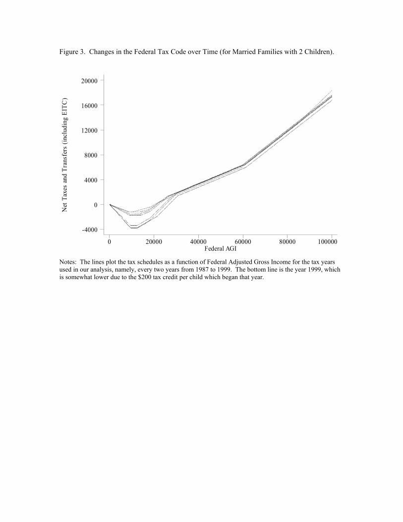
Figure 3. Changes in the Federal Tax Code over Time (for Married Families with 2 Children).

Net

Tax

es a

nd T

rans

fers

(inc

ludi

ng E

ITC

)

Federal AGI0 20000 40000 60000 80000 100000

-4000

0

4000

8000

12000

16000

20000

Notes: The lines plot the tax schedules as a function of Federal Adjusted Gross Income for the tax years used in our analysis, namely, every two years from 1987 to 1999. The bottom line is the year 1999, which is somewhat lower due to the $200 tax credit per child which began that year.

Figu

re 4

. A

vera

ge E

ITC

Pay

men

t ove

r Tim

e by

Mat

erna

l Cha

ract

eris

tics,

Bas

ed o

n La

gged

Inco

me.

0

200

400

600

800

1000

1200

1400

1600

1800

1988

1990

1992

1994

1996

1998

2000

Surv

ey Y

ear

Average EITC Payment(inflated to year 2000 dollars)

Bla

ck o

r His

pani

cW

hite

Hig

h Sc

hool

or L

ess

Som

e C

olle

ge o

r Mor

eN

ot M

arrie

dM

arrie

d2+

Chi

ldre

n1

Chi

ld