The Impact of CO , H O and Other “Greenhouse Gases” on ...

International Journal of Atmospheric and Oceanic Sciences 2021; 5(2): 29-40 http://www.sciencepublishinggroup.com/j/ijaos doi: 10.11648/j.ijaos.20210502.12 ISSN: 2640-1142 (Print); ISSN: 2640-1150 (Online)

The Impact of CO2, H2O and Other “Greenhouse Gases” on Equilibrium Earth Temperatures

David Coe1, *

, Walter Fabinski2, Gerhard Wiegleb

3 1Retired from Codel International Ltd, Bakewell, England 2Retired from ABB Automation, Frankfurt, Germany 3Department of Electrical Engineering (Research Group for Environmental Monitoring), University of Applied Sciences Dortmund, Dortmund,

Germany

Email address:

*Corresponding author

To cite this article: David Coe, Walter Fabinski, Gerhard Wiegleb. The Impact of CO2, H2O and Other “Greenhouse Gases” on Equilibrium Earth Temperatures. International Journal of Atmospheric and Oceanic Sciences. Vol. 5, No. 2, 2021, pp. 29-40. doi: 10.11648/j.ijaos.20210502.12

Received: August 2, 2021; Accepted: August 11, 2021; Published: August 23, 2021

Abstract: It has long been accepted that the “greenhouse effect”, where the atmosphere readily transmits short wavelength incoming solar radiation but selectively absorbs long wavelength outgoing radiation emitted by the earth, is responsible for warming the earth from the 255K effective earth temperature, without atmospheric warming, to the current average temperature of 288K. It is also widely accepted that the two main atmospheric greenhouse gases are H2O and CO2. What is surprising is the wide variation in the estimated warming potential of CO2, the gas held responsible for the modern concept of climate change. Estimates published by the IPCC for climate sensitivity to a doubling of CO2 concentration vary from 1.5 to 4.5°C based upon a plethora of scientific papers attempting to analyse the complexities of atmospheric thermodynamics to determine their results. The aim of this paper is to simplify the method of achieving a figure for climate sensitivity not only for CO2, but also CH4 and N2O, which are also considered to be strong greenhouse gases, by determining just how atmospheric absorption has resulted in the current 33K warming and then extrapolating that result to calculate the expected warming due to future increases of greenhouse gas concentrations. The HITRAN database of gaseous absorption spectra enables the absorption of earth radiation at its current temperature of 288K to be accurately determined for each individual atmospheric constituent and also for the combined absorption of the atmosphere as a whole. From this data it is concluded that H2O is responsible for 29.4K of the 33K warming, with CO2 contributing 3.3K and CH4 and N2O combined just 0.3K. Climate sensitivity to future increases in CO2 concentration is calculated to be 0.50K, including the positive feedback effects of H2O, while climate sensitivities to CH4 and N2O are almost undetectable at 0.06K and 0.08K respectively. This result strongly suggests that increasing levels of CO2 will not lead to significant changes in earth temperature and that increases in CH4 and N2O will have very little discernable impact.

Keywords: Carbon Dioxide, Climate Sensitivity, Greenhouse Effect, Climate Change

1. Introduction - Equilibrium Climate

Sensitivity

Equilibrium Climate Sensitivity (ECS) is generally understood to be the increase in earth surface temperature resulting from a doubling of atmospheric CO2 levels after thermal equilibrium has been achieved (Zhong and Haigh 2013) [1]. Values for ECS deduced from a variety of climate models show a high degree of uncertainty with a typical range

of 1.5 to 4.5°C (AR5-WG1-SPM, p16) [2]. More recent work, however, suggests ECS values of less than 1degC (Harde-2017) [3] (Wijngaarden and Happer 2020) [4].

The difficulty is that there are countless atmospheric variables which can be judged to have an impact upon this value. This situation is neatly summed up in the note by the UK MET Office, “What is Climate Sensitivity?” (metoffice.gov.uk).

“As there is no ‘perfect’ way of estimating climate sensitivity, it remains a hotly debated area of science and there

International Journal of Atmospheric and Oceanic Sciences 2021; 5(2): 29-40 30

remains a wide range of estimates of what the ECS could be.” This is an unfortunate situation since world governments

are implementing ambitious and expensive plans to limit the increase of global temperatures by reduction of CO2 emissions to atmosphere, and to achieve a net zero carbon economy, in the belief that CO2 emissions are the main driver of global temperature increases. In order to justify such a fundamental change to the global economy and indeed the associated risk to an “established way of life” it is of paramount importance that an accurate value for ECS is determined. To do this, it will be necessary to cut a swathe through the complexities of atmospheric thermodynamics and find a simple method of accurately estimating ECS.

1.1. The “Greenhouse Effect”

The average temperature of the earth is determined solely by the energy balance at the top of the atmosphere (TOA). At equilibrium, energy input from the sun is balanced by the energy radiating from the earth, which is a function of its temperature. The term “greenhouse effect” is used to describe the process whereby short wavelength solar radiation is transmitted through the atmosphere, whereas components of the long wavelength radiation emitted by the earth are absorbed by the atmosphere, thus limiting reradiation into space with a consequential warming of the earth (Schwartz 2018) [5, 6]. The atmospheric gases which absorb this energy, principally CO2 and H2O, are collectively referred to as “greenhouse gases”. In order to quantify this warming, it is first necessary to identify the key contributing variables.

1) Solar Radiation. This is the radiated energy received by the earth from the sun. It may be calculated from a knowledge of the sun surface temperature and the diameter and distance of the earth from the sun. This value is corroborated by direct measurement from orbital satellites. (Trenberth et al 2009) [7].

2) Earth’s Albedo. The earth’s reflectivity to solar radiation. This is a measurement of how much of the solar radiation is reflected into space, thus weakening the solar radiation input.

3) Earth’s Emissivity. All bodies emit thermal radiation as a function of their temperature according to the Planck equation for black body emission. The emissivity of the earth determines what fraction of that black body radiation is actually emitted by the earth.

4) Atmospheric Absorption. Absorption of the long wavelength radiation emitted from the earth by atmospheric gases, in particular H2O and CO2, both possessing strong infra-red radiation absorption characteristics.

5) Retention of Absorbed Energy. This is the key issue which contributes much to the uncertainty in determination of climate sensitivity. What happens to the energy absorbed by the atmosphere? There are only two possibilities; some of the energy is reradiated through to space by the warmed atmosphere, or the energy is retained by the earth and its atmosphere thus contributing to the planetary warming. This energy retention is a function of complex atmospheric thermodynamics and its estimation is a major cause of the

wide variations in climate sensitivity estimations.

1.2. Retained Energy

Variables 1 to 4 in the list above are all easily identifiable and may be determined with reasonable accuracy. Variable 5, Retention of Absorbed Energy, however, is in a different league. Atmospheric thermodynamics are immensely complicated and to use them to determine an accurate estimate of the fraction of absorbed energy that is retained is near impossible in the non-linear chaotic system that is the earth’s atmosphere and is the primary contributor to the wide range of estimates of climate sensitivity (Stevens B. et. al., 2016) [8]. There is, however, an alternative method of determining this retained energy factor using the calculations of earth temperature.

1.3. Effective Earth Temperature Te

If I0 is the energy flux received by earth from the sun, the total incident energy will be I0∙πr2, where “r” is the radius of the earth. A fraction “f” of this energy will be reflected by the earth into space (earth’s albedo). The energy received by the earth is then (1 – f)∙I0∙πr2. The energy R radiated by the earth as a result of its temperature T will be e ∙E ∙4πr2 (energy radiated over the complete earth surface of 4πr2), where “e” is the earth emissivity. E, the emissive power, is readily calculated from the Stefan Boltzmann equation

E=σT4 σ is Stefan’s constant

At equilibrium, energy received is equal to the energy emitted to space, so that

(1 – f)∙I0∙πr2=e∙σT4∙4πr2

And therefore

T=�(��)∙��∙

� (1)

This value, known as the Effective Earth Temperature Te, is generally agreed to be 255 Kelvin. This is the equilibrium earth temperature for a zero-atmosphere condition, where no absorption of the radiated energy occurs (Wilson and Gea-Banacloche 2012) [9].

1.4. The Impact of Retained Energy

The effect of an atmosphere of infra-red absorbing gases is that some of the emitted radiation will be absorbed by the atmosphere. Let “a” be the total radiative absorptivity of the atmosphere. The energy absorbed will be a∙R and the energy transmitted through to space will be (1 – a)∙R. What happens to this absorbed energy? Some will be retained by the atmosphere/earth system and some will be reradiated by the atmosphere through to space. Let “n” represent the “energy retention factor”, the fraction of the absorbed energy a∙R that is retained by the atmosphere/earth system, so that the fraction transmitted to space is (1 – n)∙a∙R. The total energy now transmitted to space is

31 David Coe et al.: The Impact of CO2, H2O and Other “Greenhouse Gases” on Equilibrium Earth Temperatures

Total energy transmitted=(1 – a)·R + (1 – n)·a·R

=(1 – n·a)·R

And for equilibrium at the TOA

(1 – f)·I0·πr2=(1 – n·a)· e·σT4·4πr2

So that equilibrium temperature T=� ��·��· ��·��

�

Therefore

T=��

√��·�� (2)

since from (1), the term T=��·��· � is already established as

the effective earth temperature of 255K. This equation applies for all atmospheric conditions,

including any effect due to atmospheric absorption of incoming solar radiation and the average impact of cloud cover. The temperature is influenced by just two variables, atmospheric absorptivity “a” and the energy retention factor “n”. Atmospheric absorptivity “a” may be calculated from a knowledge of gaseous composition, atmospheric “thickness” and the infra-red absorption spectra of those gases. Designating the total absorptivity of the current atmospheric condition as “a0” and re-arranging (2) gives the result

n.a0=(1 – (255/T)4)

Without any knowledge of, or assumptions about, atmospheric thermodynamics, the value of “n” can be ascertained from the current Equilibrium Earth Temperature T, usually considered to be 288K so that

n·a0=(1 – (255/288)4)

n·a0=0.385

This value represents the total fraction of the radiated energy which is absorbed and retained by the earth/atmosphere system, leaving 61.5% of the radiated energy transmitted through to space (Wilson and Gea-Banacloche 2012) [9]. The energy retention factor “n” is then determined from a knowledge of the total absorptivity a0 of the current atmosphere.

n=0.385/a0 (3)

This result does not suggest that “n” is a function of atmospheric absorption “a”. It is simply a method of using a known boundary condition, that is the current earth temperature and atmospheric absorption “a0” due to the current composition of greenhouse gases, to determine the unknown variable “n”.

By determining “n” it is then possible to evaluate with some accuracy, from a knowledge of the infra-red absorption characteristics of the atmosphere, how variations in atmospheric composition, particularly CO2, will impact on atmospheric absorptivity and consequently, the earth temperature. This results in a precise assessment of climate

sensitivity not only to CO2, but other radiation absorbing gases such as CH4 and N2O as well as an estimation of the feedback effects of H2O. It is first necessary however to calculate the absorptivity “a0” for the current atmospheric concentrations of H2O, CO2, CH4 and N2O.

Figure 1. Spectral radiance v Wavelength µm for a black body radiator at

288Kelvin.

2. Atmospheric Absorptivity

2.1. Spectral Radiance

Incoming radiation from the sun is predominantly short wavelength visible and near infra-red radiation. This passes through the atmosphere without significant absorption. The radiation from the earth however is purely a function of its temperature and is readily calculated by the Planck equation

Spectral Radiance Lλ=c1λ-5/(exp(c2/λT) – 1) W/m3 (4)

Whereλ is the wavelength of emitted radiation, c1 and c2 are the radiation constants. Figure 1 shows the spectral radiance from a body at a temperature of 288K, the average temperature of the earth’s surface. The radiation extends over a wide range of wavelengths from 3 to 100 µm (10-6 m).

2.2. HITRAN Database

In order to assess the impact of atmospheric greenhouse gases, it is necessary to be able to calculate exactly what fraction of the radiated energy is absorbed by differing concentrations of those gases, particularly CO2, H2O, CH4 and N2O throughout this radiation spectrum. For this a web database known as HITRAN (I. E. Gordon et al 2017) [10] has been invaluable.

The HITRAN database tabulates the transmissivity of a wide variety of gases over a range of concentrations, pressure and temperature throughout this spectral range of the radiated energy. The gases of interest are principally CO2 and H2O, being the abundant atmospheric “greenhouse gases”, and CH4 and N2O as minor atmospheric constituents. A “greenhouse gas” is defined simply as one which can absorb infra-red energy within this spectral range of 3 to 100µm.

The atmosphere, however, is not a uniform medium. As altitude increases, pressure, temperature and gas density all decrease, with the result that the transmissivity of infra-red


radiation through the atmosphere varies with altitude. Additionally, H2O concentrations are a function of the saturated vapour pressure (SVP) of water which determines how much gaseous H2O can be held by the atmosphere. SVP is also a function of temperature and therefore of altitude.

2.3. Atmospheric Altitude Variation

The variation with altitude of pressure, temperature and SVP are calculated using the following formulae.

2.3.1. Temperature

Temperature reduces at the adiabatic lapse rate of 6.5K/km to a temperature of 216K at 11000m and then remains relatively constant to 35000m.

2.3.2. Pressure

Atmospheric pressure variation with altitude can be represented by the approximation

P(alt)=P0(1 – L.h/T0)(g.M/RL)

Where P(alt) is Pressure at altitude (pascals) P0 is Pressure at sea surface (pascals) L is Adiabatic Lapse Rate (-0.0065K/m) h is Altitude (m) g is Acceleration due to gravity (9.807m/s2) M is Molar mass of dry air (0.029kg/mol) R is Gas Constant (8.314J/mol.K) See Figure 2 (US Standard Atmosphere 1976) [11].

Figure 2. Estimated atmospheric pressure variation with altitude used in the

HITRAN transmissivity downloads.

2.3.3. H2O Concentration

The concentration of water vapour is governed by the Saturation Vapour Pressure (SVP) which is a unique function of temperature. SVP is the maximum amount of water vapour that can exist without precipitating out into liquid water, i.e. cloud and rain. Actual average values of water vapour concentration are always lower than the SVP and are usually represented by the term Relative Humidity (RH) which is % of SVP. A value of 80%RH is generally assumed for average atmospheric water content, although local levels can be found across the globe varying anywhere from almost zero to 100%.

2.3.4. Saturation Vapour Pressure (SVP)

The following empirical “Buck” equation has been used to calculate SVP(kPa) (A. L. Buck 1981) [12].

SVP=0.61121exp((18.678 – T/234.5)(T/(257.14 + T)) (5)

where T is temperature in degree Celsius Figure 3 shows the variation of water vapour concentration

with an RH of 80% at atmospheric altitudes up to 35000m. As can be seen water vapour concentration drops to almost zero above 10,000m.

Figure 3. Altitude variation of H2O concentration at 80%RH.

2.3.5. CO2, CH4 and N2O Concentration

Unlike water vapour, the mean CO2 concentration will remain constant at all atmospheric levels, although its density will reduce as altitude increases and pressure and temperature decrease. CO2 concentration however will vary considerably with location and with seasons, as biospheric photosynthesis removes substantial seasonal amounts of CO2 from the atmosphere. A mean level of 400ppm has been assumed for the following calculations of atmospheric absorptivity. Similarly, CH4 and N2O concentrations will be considered to remain constant at current average levels of 1.8ppm and 0.32ppm respectively.

2.4. Calculation of Absorptivity

As can be seen from the previous graphs, pressure, temperature and water vapour concentration vary with altitude, particularly in the lower levels below 10,000m. In order to take account of these variations, the HITRAN data base has been used to calculate the transmission of radiated energy in the wavelength range 3 to 100µm through each 100m section of the atmosphere from 0 to 35000m altitude, taking into account the variations of temperature, pressure and SVP.

Let tλ.co2.h represent the transmissivity of the gas CO2 at a specific wavelength λ at the altitude “h”. Similar representations will be made for the other gasses’ H2O, CH4, N2O. The values of tλCO2.h for the temperature and pressure conditions at the specific altitude h and CO2 concentration of 400ppm are determined from the HITRAN database. The aggregate transmissivity thn to altitude level hn at the wavelengthλ is then found by:


tλ.CO2.hn=tλ.CO2.h1· tλCO2.h2·……..tλ.CO2.hn

=Πm(tλ.CO2.hm) for m=1 to n

The combined transmissivity at wavelength λ for multiple gases is found from

tλ.CO2.H2O.CH4.N2O.hn=(tλ.CO2.h1·tλ.H2O.h1·tλ.CH4.h1·tl.N2O.h1) x (tλ.CO2.h2·tλ.H2O.h2·tλ.CH4.h2·tλN2O.h2) x…………..

(tλ.CO2.hn·tλ.H2O.hn·tλ.CH4.hn·tλ.N2O.hn)

=Πm(tλ.CO2.hm·tλ.H2O.hm.·tλ.CH4.hm·tλ.N2O.hm) for m=1 to n

HITRAN data is presented in terms of wavenumber, which is the reciprocal of wavelength, in units of cm-1, a preferred unit in the field of spectroscopy. To obtain the total transmissivity over the wavenumber band 10 to 3333cm-1 (equivalent to 3 to 100µm wavelength), it is necessary to integrate the tλ’s over the entire waveband of 10 to 3333cm-1.

It is also important to decide the resolution in terms of wavenumber for the determination of the values of “tλ”. The higher the resolution the more accurate will be the final answers, but at the expense of increased computational resource. There is a resolution limit however in that pressure broadening of the individual absorption lines tends to smooth the spectral lines as resolution increases. A compromise spectral resolution of 0.1 cm-1 has been used for these calculations (Harde 2013) [13, 14] To determine the actual transmission of radiated energy at the wavelength λthrough the atmosphere it is a matter of multiplying the transmissivities tλ by the spectral radiance Lλ (4) at the wavelength λ. Transmitted Radiation Eλ at wavelength λis provided by

Eλ=(Πm(tλCO2.hm·tλ.H2O.hm.·tλCH4.hm·tλ.N2O.hm·Lλ) W/m3 for m=1 to 350 (35000m)

The total energy transmitted EE through the atmosphere is determined by integrating the radiation Eλ over the wavelength range 3 to 100µm

EE=Σλ(Eλ· ∆λ W/m2 for λ=3.0 to 100.0µm

where ∆λ is the wavelength increment at wavelength λ equivalent to the wavenumber increment of 0.1cm-1, which is the resolution chosen for the HITRAN data. The atmospheric transmissivity is then calculated from EE/σT4.

Figure 4. Spectral Transmission through the atmosphere of 400ppm CO2 v

Wavelength µm.

2.5. Atmospheric Absorption Spectra for CO2 and H2O

Figures 4, 5 and 6 show the transmission of the spectral radiation Eλ, through current atmospheric concentrations of CO2 and H2O and through the combination of the two gases. Absorptivities of both CO2 and H2O, as well as CH4 and N2O, have been determined over the range 3 to 100µm to a resolution of 0.1cm-1. It is clear that significant amounts of radiated energy are absorbed by both CO2 and H2O. It is also clear that there is considerable overlap of the absorption bands of CO2 and H2O with the H2O absorption being the dominant factor.

Figure 5. Spectral Transmission through the atmosphere of H2O v Wavelength

µm.

Figure 6. Combined CO2 + H2O Spectral Transmission through the

atmosphere v Wavelength µm.

Figure 7. Atmospheric absorptivity variation with altitude.

It is also possible to calculate the absorption of energy as it


passes from sea level to 35000m as shown in Figure 7. As can be seen, most of the radiation absorption occurs in the lower 5000m of the atmosphere. Beyond that point the radiation in the CO2 and H2O absorption bands has been absorbed and reduced to almost zero. Little further absorption can occur. The calculations and this graph show the total atmospheric absorptivity due to H2O and CO2 to be 72.6%, with the dominant absorber, H2O, contributing 67.0% while the impact of 400ppm CO2 provides the additional 5.6%. Note that without the presence of H2O, the absorption due to CO2 would be 18%. The overlapping spectral absorption bands of the dominant H2O molecules reduce the CO2 impact to 5.6%.

2.6. Impact of Methane (CH4) and Nitrous Oxide (N2O)

CH4 and N2O are recognized as strong absorbers of long wavelength infra-red energy and are considered to be significant contributors towards global warming. It is claimed that CH4 has a global warning potential 86 times stronger per unit mass than CO2 (Etminan, Myhre, Highwood and Shine, 2016) [15].

2.6.1. Current Atmospheric Concentrations 1.8ppm CH4 and

0.32ppm N2O

The spectral transmissions of 1.8ppm CH4 and 0.32ppm N2O, are also calculated using HITRAN data base and are shown in Figures 8 and 9. All the infra-red absorption for these two gases occurs at wavelengths below 20µm. When total atmospheric infra-red transmission, including.

Figure 8. Spectral Transmission through the atmosphere of 1.8ppm CH4 v

Wavelength µm.

Figure 9. Spectral Transmission through the atmosphere of 0.32ppm N2O v

Wavelength µm.

Figure 10. Total Spectral Transmission CH4 + N2O + CO2 + H2O through the

atmosphere v Wavelength µm.

CH4 and N2O is shown in figure 10, superimposed over the transmission through H2O and CO2 alone, it is immediately clear that the impact of both CH4 and N2O is almost completely swamped by the combined overlapping absorption bands of H2O and CO2. Nevertheless, there is a small measurable effect in that the total atmospheric absorptivity is increased from 72.6% to 73.0%, an increase of 0.4%, by the contribution of these two gases at current atmospheric concentrations.

Figure 11. Atmospheric absorptivity variation with CH4 and N2O

concentration.

2.6.2. Increasing Concentrations of CH4 and N2O

CH4 and N2O are indeed very powerful absorbers of infra-red radiation. Increasing the concentrations of each gas to 30ppm (a 16fold increase in the case of CH4 and an almost 100fold increase in N2O) would result in a combined absorption of 15%, close to the value of 18% for 400ppm of CO2. The combined absorptive impact in the presence of H2O and CO2 however reduces this absorption to less than 3% as can be seen in Figure 11 due to the overlap of the absorption bands of CO2 and H2O. It would thus take a huge increase in atmospheric concentrations of these gases to have any significant impact on total atmospheric infra-red absorption.

2.7. Retention of Absorbed Energy

The calculated value of 0.730 for the absorption of the earth’s radiated energy for the current average atmospheric


condition (400ppm CO2, 80% Relative Humidity, 1.8ppm CH4, 0.32ppm N2O and temperature 288K), allows us to determine, without any assumption or even knowledge of the complex atmospheric thermodynamics, the fraction “n” of absorbed energy which is retained by the earth.

Figure 12. Total atmospheric radiation transmission and retained absorption.

Sector 1 Blue % Radiated energy transmitted to space 61.5% Sector 2 Orange % Radiated energy absorbed by CO2 3.0% Sector 3 Grey % Radiated energy absorbed by H2O 35.3% Sector 4 Yellow % Radiated energy absorbed by CH4 + N2O 0.2%

From (3) n=0.385/a0 While a0=0.730 Thus n=0.5274 This suggests that only 52.74% of the radiated energy

absorbed by the atmosphere is actually retained by the earth/atmosphere system. So, the net retention of the radiated energy is 52.74% of 73.0%=38.5%, leaving 61.5% of radiated energy being transmitted to space to balance the solar energy input and produce an average earth temperature of 288 Kelvin. The total absorption and transmission of radiated energy is summarised in the pie chart of Figure 12.

By calculating the absorptivity “a” for a range of atmospheric gas concentrations using the HITRAN database, the earth temperature T can now be determined from (2) by substituting n=0.5274. so that

T=��

√��.��·�� Kelvin (6)

allowing an accurate assessment of climate sensitivity to variations in atmospheric absorptivity and hence to concentration of “greenhouse gases”.

Table 1. Variation of atmospheric absorptivity with CO2 concentration.

CO2 ppm 0 10 50 100 200 400 800 1600

CO2 Absorption % 0.0 9.7 13.5 15.2 17.0 18.7 20.4 22.3

Total Absorption % 67.7 70.2 71.2 71.8 72.4 73.0 73.0 74.6

Figure 13. Atmospheric absorptivity v ppm CO2.

3. Atmospheric Impact on Equilibrium

Earth Temperatures

3.1. Variation of Total Absorptivity with Atmospheric CO2

Concentration

Repeating the calculation procedure using HITRAN data for CO2 concentrations from 50ppm through to 1600ppm results in the data in Table 1 and Figure 13 for total absorption which includes the absorption due to H2O, 1.8ppm CH4 and 0.32ppm N2O.

3.2. Variation of Equilibrium Earth Temperature with CO2

Concentration

Using (5) T=��

√��.��·�� Kelvin

The corresponding temperature changes, as absorptivity varies with CO2 concentration, are as shown in the following Table 2 and Figure 14. Increasing CO2 concentrations from the current 400ppm to 1600ppm will increase global temperatures from 288K to 289K, an increase of just 1Kelvin.

Table 2. Variation of earth equilibrium temperature with CO2 concentration,

assuming all other atmospheric constituents remain at their current values.

CO2 ppm 10 50 100 200 400 800 1600

Temperature Kelvin 284.8 286.2 286.9 287.6 288.0 288.4 289.0

Figure 14. Earth Temperature variation with CO2 concentration.


3.3. Variation of Equilibrium Earth Temperature with CH4

and N2O Concentration

3.3.1. CH4 Methane

The absorptivity of methane in the atmosphere at concentrations up to 28.8ppm, 16 times current atmospheric levels, is calculated using HITRAN data and is shown in Table 3. Also, in Table 3 are the total atmospheric absorption levels, including the impact of current atmospheric levels of CO2, H2O and N2O and the resulting equilibrium temperature calculated using (5).

Table 3. Variation of atmospheric absorptivity and earth temperature with

variation in CH4 concentration up to 16 times the current level of 1.8ppm.

ppm CH4 1.8 3.6 7.2 14.4 28.8

CH4 absorption % 1.6 2.1 2.8 3.7 4.7 Total absorption % 73.03 73.1 73.22 73.36 73.54 Temperature Kelvin 287.97 288.02 288.09 288.17 288.28

Table 4. Variation of atmospheric absorptivity and earth temperature with

variation in N2O concentration up to 16 times the current level of 0.32ppm.

ppm N2O 0.32 0.64 1.28 2.56 5.12

N2O absorption % 1.7 2.6 3.8 5.4 7.3 Total absorption % 73.03 73.14 73.30 73.54 73.87 Temperature Kelvin 287.97 288.04 288.14 288.28 288.49

3.3.2. N2O Nitrous Oxide

Similar HITRAN calculations for N2O concentrations up to 5.1ppm, again 16 times current atmospheric levels of 0.32ppm, are provided in Table 4 showing the impact on absorptivity and temperature.

While both CH4 and N2O are both recognised as strong absorbers of infra-red radiation their impact is muted by the dominant H2O radiation absorption to the point that an unlikely 16fold increase in concentrations would result in an increase in the earth’s temperature of 0.3K due to CH4 and 0.5K due to N2O.

3.4. The Impact of H2O

The maximum H2O concentration that can be held in the atmosphere is a direct consequence of temperature and is governed by the saturated vapour pressure. Actual H2O concentrations are mostly lower than this maximum value, represented by the fraction “Relative Humidity” RH. An RH of 0.8 has been assumed throughout for these calculations. It would be useful to determine what impact variations in RH will have upon atmospheric absorption and earth temperatures. The results of calculations of RH variations from 0.6 through to 1.0 are provided in Table 5 and Figures 15 and 16. A variation in Relative Humidity of +/- 20% results in a variation of average earth temperature of +/- 0.6K.

Table 5. The impact of variations in mean relative humidity RH on

atmospheric absorptivity and earth temperature.

Relative Humidity % 0.6 0.7 0.8 0.9 1.0

H2O absorption % 65.1 66.1 67.0 67.8 68.6 Total absorption % 72.0 72.5 73.0 73.5 73.9 Temperature Kelvin 287.3 287.7 288.0 288.2 288.5

This is, at first sight, a surprisingly low temperature variation, until the realisation sets in that the main H2O absorption bands are already well saturated, in that almost all the infra-red energy in those bands has already been absorbed. Changes in H2O concentration have little further impact.

Figure 15. Atmospheric absorptivity variation with average earth Relative

Humidity.

Figure 16. Earth Temperature variation with Relative Humidity.

3.5. Water Vapour Feedback

It is often claimed that increasing temperatures due to increasing CO2 levels will result in a positive feedback since the SVP of H2O will also increase thus enabling the atmosphere to retain higher levels of moisture, giving rise to significantly higher climate sensitivity values (Held and Soden 2000) [16].

Assume a temperature increase ∆T0 for whatever reason. That increase will result in an increase in H2O saturated vapour pressure and an increase in H2O concentration ∆H2O, proportional to the temperature increase. ∆H2O=j·∆T0 where “j” is the concentration proportionality constant.

In turn, the increased concentration will increase infra-red absorption resulting in a further increase in temperature ∆T1 proportional to ∆H2O.

∆T1=k · ∆H2O “k” is the temperature proportionality constant.

Thus ∆T1=j·k·∆T0 Of course, this temperature increase ∆T1 will itself produce

a further temperature increase ∆T2 where

∆T2=j·k·∆T1=(j·k)2 ∆T0

And so on, resulting in a total temperature increase

∆T=∆T0 + ∆T1 + ∆T2 +…... ∆Tn +…….


=∆T0·Σn(j·k)n for n=0 to ∞

Σn(j·k)n is an infinite series that, if (j·k) � 1, will diverge and the atmospheric system will be unstable, and the earth uninhabitable. If (j.k) is < 1 the series will converge, and the impact of H2O will be to amplify the original temperature increase ∆T0. The question now is by how much?

To answer this, numerical values must be allocated to the coefficients, “j” and “k”. Differentiating the equation for SVP (5) with respect to T, provides values for the SVP sensitivity to temperature d(SVP)�dT (Figure 17).

From this data for SVP variation with temperature a value for “j” can be allocated. Since temperature, and thus SVP reduce with altitude, the sensitivity of SVP to changes in temperature d(SVP)�dT also varies with altitude. However, from Figure 17 it is easy to see that the lower altitude levels of the atmosphere have by far the strongest effects on absorptivity. A realistic, and indeed worst case, value for the constant “j” would be the value at sea level, which is

j=0.088%�K

Figure 17. Rate of change of Saturated Vapour Pressure with Temperature v

Altitude.

For “k” it is necessary to look first at Figure 16, which shows temperature change for variations in RH value. Specifically, it is clear that an RH variation from 0.6 to 1.0 results in an almost linear temperature change of 1.2K. From Figure 4 the H2O concentration at sea level assuming 80% RH is 1.36%. Thus a change of RH from 0.6 to 1.0 results in a change in concentration of 0.68%.

Thus k=1.2K�0.68%=1.765 K�%H2O And so, j·k=0.088 x 1.765=0.155 This results in the infinites series Σn(j·k)n converging to a

value of 1.183, which becomes an amplification factor due to H2O for any change in temperature in Kelvin, for any reason.

3.6. Temperature Feedback

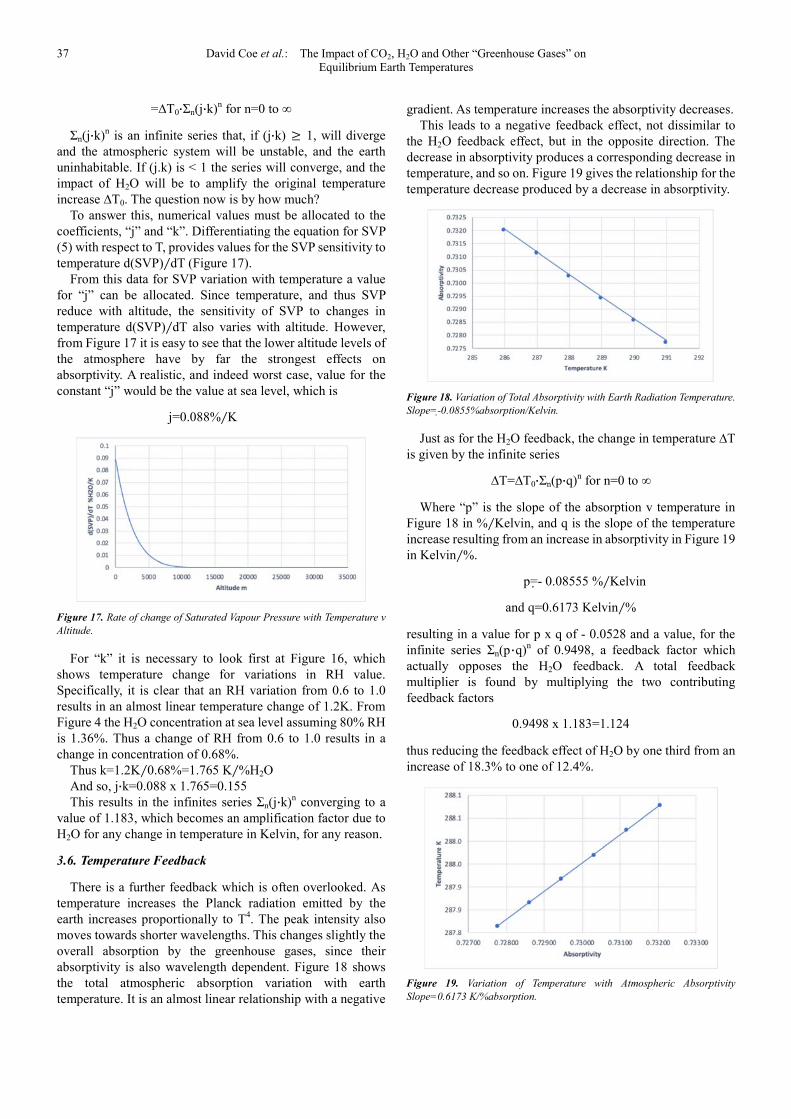
There is a further feedback which is often overlooked. As temperature increases the Planck radiation emitted by the earth increases proportionally to T4. The peak intensity also moves towards shorter wavelengths. This changes slightly the overall absorption by the greenhouse gases, since their absorptivity is also wavelength dependent. Figure 18 shows the total atmospheric absorption variation with earth temperature. It is an almost linear relationship with a negative

gradient. As temperature increases the absorptivity decreases. This leads to a negative feedback effect, not dissimilar to

the H2O feedback effect, but in the opposite direction. The decrease in absorptivity produces a corresponding decrease in temperature, and so on. Figure 19 gives the relationship for the temperature decrease produced by a decrease in absorptivity.

Figure 18. Variation of Total Absorptivity with Earth Radiation Temperature.

Slope=-60.0855%absorption/Kelvin.

Just as for the H2O feedback, the change in temperature ∆T is given by the infinite series

∆T=∆T0·Σn(p·q)n for n=0 to ∞

Where “p” is the slope of the absorption v temperature in Figure 18 in %�Kelvin, and q is the slope of the temperature increase resulting from an increase in absorptivity in Figure 19 in Kelvin�%.

p=- 0.08555 %�Kelvin

and q=0.6173 Kelvin�%

resulting in a value for p x q of - 0.0528 and a value, for the infinite series Σn(p·q)n of 0.9498, a feedback factor which actually opposes the H2O feedback. A total feedback multiplier is found by multiplying the two contributing feedback factors

0.9498 x 1.183=1.124

thus reducing the feedback effect of H2O by one third from an increase of 18.3% to one of 12.4%.

Figure 19. Variation of Temperature with Atmospheric Absorptivity

Slope=0.6173 K/%absorption.


4. Equilibrium Climate Sensitivity

It is now possible to infer meaningful and accurate values for climate sensitivities to all “greenhouse gases” defined as the change in average earth temperature upon reaching equilibrium from the effects of a doubling of the gas concentration.

4.1. Climate Sensitivity to CO2

From section 3.2 Table 2 shows the variation of equilibrium temperature for successive doublings of CO2 concentration from 50ppm through to 1600ppm. The corresponding changes in temperature for each doubling are readily calculated in Table 6 and are shown in Figure 20. As can be seen “climate sensitivity” is not constant, but slowly increases with increasing CO2 concentrations. Nevertheless, the values indicate that climate sensitivity at current CO2 levels (400ppm) is of the order of 0.45 Kelvin. Applying the combined feedback H2O and temperature multiplying factor of 1.124, increases the CO2 climate sensitivity to 0.50 Kelvin, still significantly lower than most published values.

Table 6. CO2 Climate Sensitivity.

CO2 ppm doubling 50-100 100-200 200-400 400-800 800-1600

Climate sensitivity K 0.34 0.38 0.41 0.45 0.54

Sensitivity x feedback K 0.38 0.42 0.46 0.50 0.61

Figure 20. Climate Sensitivity to CO2.

4.2. Climate Sensitivity to CH4 and N2O

Section 3.3 provides the data for changes in earth temperature for successive doublings of the concentrations of CH4 and N2O.

Methane CH4:- Table 7 and Figure 21

Table 7. CH4 Climate Sensitivity.

CH4 ppm doubling 1.8-3.6 3.6-7.2 7.2-14.4 14.4-28.8

Climate sensitivity K 0.05 0.07 0.09 0.11

Sensitivity x feedback K 0.06 0.08 0.10 0.12

Figure 21. Climate Sensitivity to CH4.

Nitrous Oxide N2O:-Table 8 and Figure 22

Table 8. N2O Climate Sensitivity.

N2O ppm doubling 0.32-0.64 0.64-1.28 1.28-2.56 2.56-5.12

Climate sensitivity K 0.07 0.10 0.15 0.21

Sensitivity x feedback K 0.08 0.11 0.16 0.23

Figure 22. Climate Sensitivity to N2O.

It is clear that climate sensitivity for these two gases is not a constant. It increases with concentration, for the simple reason that at these low concentrations the main radiation absorption bands are not yet saturated. At current atmospheric levels of 1.8ppm CH4 and 0.32ppm N2O the current climate sensitivities including feedback effects are 0.06 and 0.08 Kelvin respectively. While both gases are described as strong greenhouse gases their actual impact upon earth temperatures at current concentration levels is actually so small as to be almost unmeasurable.

5. Other Considerations

5.1. The Impact of Clouds

The obvious impact of clouds is to increase the reflectivity of the earth thus reducing the level of incoming solar radiance I0 which will have a cooling influence on the earth. However, this paper is concerned with the effects of retained IR emissions from the earth.

Cloud cover will not affect the absorbance of atmospheric greenhouse gases, but it will impact upon the total energy


absorbed and possibly upon the energy retention factor “n”, in ways that would be difficult to quantify. However, by using the current average earth condition, which includes cloud, as a calibration point to determine an effective value for ”n” consistent with the mean earth temperature of 288K, the current average impact of cloud has, in effect, already been taken into account. This however does not, in itself, identify what this impact is.

The structure of clouds is diverse and complex. It is close to impossible to derive a set of equations to describe the formation, structure and impact of clouds on the retention of absorbed energy and hence the radiative balance of the earth. This paper has so far relied upon the extensive HITRAN spectral database, basic physics and simple mathematics to determine values for climate sensitivity. Any attempts to estimate the further impact of cloud would be based upon speculation only and would not be appropriate for this paper.

5.2. Effect of Recently Increased Atmospheric CO2

It is of some interest to calculate the increase in temperature that has occurred due to the increase in atmospheric CO2 levels from the 280ppm prior at the start of the industrial revolution to the current 420ppm registered at the Mona Loa Observatory. (K. W. Thoning et. al. 2019) [17]. The HITRAN calculations show that atmospheric absorptivity has increased from 0.727 to 0.730 due to the increase of 140ppm CO2, resulting in a temperature increase of 0.24Kelvin. This is, therefore, the full extent of anthropogenic global warming to date.

6. Conclusions

In order to satisfy radiative equilibrium at the “top of the atmosphere” (TOA) at an average earth temperature of 288Kelvin, only 61.5% of the earth’s radiated energy should be transmitted through to space, leaving 38.5% to be absorbed and retained by the atmosphere/earth. Use of the HITRAN data base of gaseous absorption spectra shows the current atmospheric absorption to be 73.0% of total radiative emissions of which 52.74% must be retained by the earth/atmosphere to satisfy the current TOA equilibrium. This is a simple expression of the current earth temperature equilibrium.

The 38.5% retained radiation absorption comprises 35.3% attributed to H2O, 3.0% to CO2 and a mere 0.2% to CH4 and N2O combined. From this it follows that the 33Kelvin warming of the earth from 255Kelvin, widely accepted as the zero-atmosphere earth temperature, to the current average temperature of 288Kelvin, is a 29.4K increase attributed to H2O, 3.3K to CO2 and 0.3K to CH4 and N2O combined. H2O is by far the dominant greenhouse gas, and its atmospheric concentration is determined solely by atmospheric temperature. Furthermore, the strength of the H2O infra-red absorption bands is such that the radiation within those bands is quickly absorbed in the lower atmosphere resulting in further increases in H2O concentrations having little further effect upon atmospheric absorption and hence earth temperatures. An increase in

average Relative Humidity of 1% will result in a temperature increase of 0.03Kelvin.

By comparison CO2 is a bit player. It however does possess strong spectral absorption bands which, like H2O, absorb most of the radiated energy, within those bands, in the lower atmosphere. It also suffers the big disadvantage that most of its absorption bands are overlapped by those of H2O thus reducing greatly its effectiveness. In fact, the climate sensitivity to a doubling of CO2 from 400ppm to 800ppm is calculated to be 0.45 Kelvin. This increases to 0.50 Kelvin when feedback effects are taken into account. This figure is significantly lower than the IPCC claims of 1.5 to 4.5 Kelvin.

The contribution of CH4 and N2O is miniscule. Not only have they contributed a mere 0.3Kelvin to current earth temperatures, their climate sensitivities to a doubling of their present atmospheric concentrations are 0.06 and 0.08 Kelvin respectively. As with CO2 their absorption spectra are largely overlapped by the H2O spectra again substantially reducing their impact.

It is often claimed that a major contributor to global warming is the positive feedback effect of H2O. As the atmosphere warms, the atmospheric concentration of H2O also increases, resulting in a further increase in temperature suggesting that a tipping point might eventually be reached where runaway temperatures are experienced. The calculations in this paper show that this is simply not the case. There is indeed a positive feedback effect due to the presence of H2O, but this is limited to a multiplying effect of 1.183 to any temperature increase. For example, it increases the CO2 climate sensitivity from 0.45K to 0.53K.

A further feedback, however, is caused by a reduction in atmospheric absorptivity as the spectral radiance of the earth’s emitted energy increases with temperature, with peak emissions moving slightly towards lower radiation wavelengths. This causes a negative feedback with a temperature multiplier of 0.9894. This results in a total feedback multiplier of 1.124, reducing the effective CO2 climate sensitivity from 0.53 to 0.50 Kelvin.

Feedback effects play a minor role in the warming of the earth. There is, and never can be, a tipping point. As the concentrations of greenhouse gases increase, the temperature sensitivity to those increases becomes smaller and smaller. The earth’s atmosphere is a near perfect example of a stable system. It is also possible to attribute the impact of the increase in CO2 concentrations from the pre-industrial levels of 280ppm to the current 420ppm to an increase in earth mean temperature of just 0.24Kelvin, a figure entirely consistent with the calculated climate sensitivity of 0.50 Kelvin.

The atmosphere, mainly due to the beneficial characteristics and impact of H2O absorption spectra, proves to be a highly stable moderator of global temperatures. There is no impending climate emergency and CO2 is not the control parameter of global temperatures, that accolade falls to H2O. CO2 is simply the supporter of life on this planet as a result of the miracle of photosynthesis.


Symbols and Abbreviations

a Atmospheric absorptivity a0 Current atmospheric absorptivity c1 1st radiation constant c2 2nd radiation constant e Earth emissivity E Emissive Power W/m2

Eλ Energy transmitted through atmosphere at wavelength λ

EE Total energy transmitted through the atmosphere f Earth albedo hn Altitude level (in 100m sections) I0 Solar Irradiance W/m2

IPCC Intergovernmental Panel on Climate Change j H2O concentration proportionality constant %/K k Temperature proportionality constant K/% K Kelvin L Spectral Radiance W/m3 p Absorption temperature coefficient %/K ppm Concentration in parts per million q variation of temperature with absorption K/% r Earth radius m R Earth radiated emission W/m2

t transmissivity tE Total energy transmitted W/m2 tλ Transmissivity at wavelength λ T Earth temperature Kelvin Te Effective earth temperature Kelvin TOA Top of the atmosphere ∆H H2O concentration incremental increase % λ Radiation wavelength µm σ Stefan’s Constant W/m2/K4

References

[1] Zhong, W. Y., and J. D. Haigh (2013), The greenhouse effect and carbon dioxide, Weather, 68 (4), 100–105, doi: 10.1002/wea.2072.

[2] G. Myhre et al, Anthropogenic and Natural Radiative Forcing, Climate Change 2013: The Physical Science Basis. Contribution of Working Group I to the Fifth Assessment Report of the Intergovernmental Panel on Climate Change. Cambridge University Press, Cambridge, United Kingdom (2013).

[3] H. Harde, Radiation Transfer Calculations and Assessment of Global Warming by CO2, International Journal of Atmospheric Sciences, Vol. 2017, Article ID 9251034.

[4] W. A. van Wijngaarden & W. Happer, Dependence of Earth’s

Thermal Radiation on Five Most Abundant Greenhouse Gases. Atmospheric and Oceanic Physics arXiv: 2006.03098 (2020).

[5] S. E. Schwartz, Resource Letter GECC-1: The Greenhouse Effect and Climate Change: Earth’s Natural Greenhouse Effect, Am. J. Phys. 86, (8), 565-576, (2018).

[6] S. E. Schwartz, Resource Letter GECC-2: The Greenhouse Effect and Climate Change: The Intensified Greenhouse Effect, Am. J. Phys. 86, (9), 645-656, (2018).

[7] K. E. Trenberth, J. T. Fasullo and J. Kiehl, “Earth’s Global Energy Budget”, Bulletin of the American Meteorological Society, vol. 90, no. 3, pp 311-323, 2009.

[8] Stevens, B., S. C. Sherwood, S. Bony, and M. J. Webb (2016), Prospects for narrowing bounds on Earth’s equilibrium climate sensitivity, Earth’s Future, 4, 512-522. Future, 4, 512–522 doi: 10.1002/2016EF000376.

[9] D. J. Wilson and J. Gea-Banacloche, Simple Model to Estimate the Contribution of Atmospheric CO2 to the Earth’s Greenhouse Effect, Am. J. Phys. 80 306 (2012).

[10] I. E. Gordon, L. S. Rothman et al., The HITRAN2016 Molecular Spectroscopic Database, JQSRT 203, 3-69 (2017).

[11] U.S. Standard Atmosphere 1976, National Oceanic and Atmospheric Administration, National Aeronautics and Space Administration, Washington, DC, USA, 1976.

[12] A. L. Buck (1981), New equations for computing vapour pressure and enhancement factor, J. Appl. Meteorol., 20: 1527-1532.

[13] Hermann Harde, "Radiation and Heat Transfer in the Atmosphere: A Comprehensive approach on a Molecular Basis", International Journal of Atmospheric Sciences, vol. 2013, Article ID 503727, 26 pages, 2013. https://doi.org/10.1155/2013/503727.

[14] H. Harde, Radiative and Heat Transfer in the Atmosphere: A Comprehensive Approach on a Molecular Basis, Int. J. Atm. Sci. 503727, (2013).

[15] M. Etminan, G. Myhre, E. J. Highwood and K. P. Shine, Radiative Forcing of Carbon Dioxide, Methane and Nitrous Oxide: A Significant Revision of the Methane Radiative Forcing, Geophys. Res. Lett. 43, 12614 (2016).

[16] I. M. Held and B. J. Soden (2000) Water Vapour Feedback and Global Warming, Annual Review of Energy and the Environment, Vol. 25:441-475 (Nov 2000).

[17] K. W. Thoning, A. M. Crotwell, and J. W. Mund (2021), Atmospheric Carbon Dioxide Dry Air Mole Fractions from continuous measurements at Mauna Loa, Hawaii, Barrow, Alaska, American Samoa and South Pole. 1973-2019, Version 2021-02 National Oceanic and Atmospheric Administration (NOAA), Global Monitoring Laboratory (GML), Boulder, Colorado, USA.

The Impact of CO , H O and Other “Greenhouse Gases” on ...

Documents

Transcript of The Impact of CO , H O and Other “Greenhouse Gases” on ...