The Impact of an Abortion Ban on Socio-Economic …cp2124/papers/unwanted_latest.pdfThe Impact of an...

The Impact of an Abortion Ban on Socio-EconomicOutcomes of Children: Evidence from Romania∗

Cristian Pop-Eleches�

Columbia University

October 2005

Abstract

This study examines educational and labor outcomes of children affected bya ban on abortions. I use evidence from Romania, where in 1966 dictator NicolaeCeausescu declared abortion and family planning illegal. Birth rates doubled in1967 because formerly abortion had been the primary method of birth control.Children born after the abortion ban attained more years of schooling and greaterlabor market success. This is because urban, educated women were more likely tohave abortions prior to the policy change, and the relative number of children bornto this type of woman increased after the ban. However, controlling for compositionusing observable background variables, children born after the ban on abortions hadworse educational and labor market achievements as adults. Additionally, I provideevidence of crowding in the schooling system and some suggestive evidence thatcohorts born after the introduction of the abortion ban had higher infant mortalityand increased criminal behavior later in life. While in the short-run the abortionban differentially increased fertility of more educated women, in the long-run theban differentially increased fertility among less educated women. This suggests thateducated women changed their behavior more drastically as a result of the ban.

∗I am especially grateful to my dissertation advisors Michael Kremer, Larry Katz, Caroline Hoxbyand Andrei Shleifer for their guidance and support. I received helpful comments from two editors, twoanonymous referees, Merriol Almond, Abhijit Banerjee, David Cutler, Rajeev Dehejia, Esther Dußo,Ed Glaeser, Claudia Goldin, Robin Greenwood, Ofer Malamud, Sarah Reber, Ben Olken, EmmanuelSaez, Tara Watson, and seminar participants at Boston University, Clemson, Columbia, Harvard, NBERSummer Institute, NEUDC, Princeton, Vanderbilt, and the World Bank. Any errors are solely mine.Financial support from the Social Science Research Council Program in Applied Economics, the Centerfor International Development and the Kokkalis Program at Harvard is gratefully acknowledged.

�Department of Economics and SIPA, Columbia University, 420West 118th Street, Rm. 1022 IABMC 3308, New York, NY 10027, [email protected]

1

1 Introduction

A number of recent studies have used the legalization of abortion in the US in the 1970�s

to analyze how the change in access to abortion affects child outcomes later in life. These

studies Þnd that the cohorts of children resulting from pregnancies that could have been

legally terminated display better socio-economic outcomes along a wide range of indica-

tors: they are less likely to live in a single household and less likely to live in poverty and

in a household receiving welfare (Gruber, Levine, and Staiger, 1999), they consume fewer

controlled substances (Charles and Stephens, 2002), have lower teen childbearing rates

(Donohue, Grogger and Levitt, 2002) and are less likely to commit crimes (Donohue and

Levitt, 2001).

This paper is also an effort to understand the link between access to abortion and socio-

economic outcomes of children, but using a major policy change in the opposite direction.

In 1966 Romania abruptly shifted from one of the most liberal abortion policies in the

world to a very restrictive regime that made abortion and family planning illegal for most

women. This policy was maintained, with only minor modiÞcations, until December 1989,

when following the fall of communism, Romania reverted back to a liberal policy regarding

abortion and modern contraceptives. The short-run impact of the 1966 change in policy

was an immediate and enormous increase in births: the total fertility rate increased from

1.9 to 3.7 children per woman between 1966 and 1967.

On average, children born in 1967 just after abortion became illegal display signiÞ-

cantly better educational and labor market achievements than children born just prior to

the change. This seemingly paradoxical result is the opposite of what one would expect in

light of the Þndings from the US, but can be explained by a change in the composition of

women having children: urban, educated women were more likely to have abortions prior

to the policy change, so a higher proportion of children were born into urban, educated

households after abortions became illegal. Controlling for this type of composition using

observable background variables, children born after the abortion ban had worse school-

ing and labor market outcomes. This Þnding is consistent with the view that children

who were unwanted during pregnancy had inferior socio-economic outcomes once they

became adults. Additionally, I provide evidence that the increase in cohort size due to

2

the abortion ban resulted in a crowding effect in the schooling system.

The Þnal part of the paper contains two extensions to the main analysis. First I show

that while in the short-run the more educated women were mostly affected by the abortion

ban, in the long-run the less educated women had the largest increases in fertility as a

result of Romania�s 23 year period (1967-1989) of continued pronatalist policies. This

implies that educated women changed their behavior more drastically as a result of the

ban and suggests that more educated women are more effective in reaching their desired

fertility when access to birth control methods is difficult. Secondly, I offer some suggestive

evidence that cohorts born after the introduction of the abortion ban had higher infant

mortality and increased criminal behavior later in life.

Following is the plan of the paper. Section 2 provides an overview of the channels

through which an unwanted birth might affect the socio-economic outcome of a child.

Section 3 describes the unusual history of abortion legislation in Romania. In section 4,

I describe the data and empirical strategy. Section 5 presents the results of the main

analysis. Section 6 includes the two extensions and section 7 concludes.

2 The mechanisms by which an abortion ban affects

socio-economic outcomes of children

Consider a woman�s decision as to whether to use birth control: if the costs of using a

certain birth control method increases substantially, she will likely use less of it. Instead,

she will rely on abstinence, use alternative birth control technologies, and/or have more

births. Thus, the children born under a restrictive birth control regime are more likely

to be unplanned, unwanted or mistimed, relative to a world where a woman exercised

costless control over her fertility. I will refer to children, whose births are a result of the

increased cost of fertility control, as �unwanted.� How might unwantedness affect adult

outcomes?

A Þrst way in which an unwanted birth might affect the quality of a child derives

from the standard model of the child quality/quantity trade-off (Becker, 1981). Since it is

assumed that parents desire equal levels of quality for each of their children, an increase

in the number of children as a result of an unwanted pregnancy leads to a decrease in

3

child quality for all children in the household.

Secondly, optimal timing of birth might play an important role in the future develop-

ment of a child. If access to birth control methods becomes difficult, women are less able

to delay childbearing until conditions are more favorable for raising children. Unfavorable

conditions might arise for a number of reasons. Childbearing can conßict with the longer

term educational and labor market plans of a mother (Angrist and Evans, 1996), which

can have a negative effect on the child. In addition a mother, who gives birth to an

unwanted child prior to marriage, might either enter an undesired marriage or face single

parenthood. Finally, a whole range of additional factors, broadly related to a mother�s

(and father�s) physical and emotional well-being resulting from involuntary parenthood

might affect the development of children within a family.

Finally, in the presence of selection in terms of pregnancy resolution, a change in

access to birth control methods can affect the average quality of children. A number of

studies (Grossman and Jacobowitz 1981; Joyce 1987; Grossman and Joyce 1990) show

that increased access to abortion increased the weight of children at birth and decreased

neonatal mortality, suggesting positive selection on fetal health.

The different theoretical channels just reviewed all predict that making access to

abortions harder will have a negative effect on a child�s development. Thus, for the

purposes of this paper, I will call the combined effect of the three channels the effect of

unwantedness on child outcomes. In addition to the mentioned US based research, the

papers by Myhrman (1988) for Finland, Bloomberg (1980) for Sweden and Dytrych et

al. (1975), David and Matejcek (1981) and David (1986) for the Czech Republic have

studied outcomes of children born to mothers who have been denied access to abortion.

Unwanted children display a number of negative outcomes, ranging from poorer health,

lower school performance, more neurotic and psychosomatic problems, a higher likelihood

of receiving child welfare, to more contentious relationships with parents and higher teen

sexual activity. The major drawback of these studies is their inability to convincingly

account for the self-selection of a certain type of mothers into the treatment group.1

1The Heckman bivariate selection model (Heckman, 1979) is the standard approach to control for non-random selection into the treatment group. Without making strong structural form assumptions, thisestimator generally needs an exclusion restriction; in this case there are no plausible exclusion restrictionsacross the selection into treatment and child outcome equations.

4

There are two additional ways through which a change in abortion legislation could

affect the average socio-economic outcome of children. First, one has to understand how

the change in policy inßuences the composition of women who carry pregnancies to term.

The direction of the effect is theoretically ambiguous and ultimately requires an empirical

analysis of which types of women are most affected by the change in policy. While the

evidence from the US (Gruber, Levine and Staiger, 1999) suggests that women from

disadvantaged backgrounds are more likely to use abortion and thus are more affected

by a change in abortion regime, the present analysis shows that in the case of Romania,

abortion was used primarily by urban, educated women.

Finally, if the fertility impact of the ban on abortions is large, one could imagine a

negative crowding effect resulting from a larger cohort competing for scarce resources.2

The importance of possible crowding effects is an interesting question of its own and will

be addressed in a later section.

3 Abortion and birth control policy regimes in Ro-

mania

Prior to 1966, Romania had one the most liberal abortion policies in Europe, since

abortions were legal in the Þrst trimester and provided at no cost by the state health care

system. Abortion was the most widely used method of birth control (World Bank, 1992)

and in 1965, there were four abortions for every live birth (Berelson, 1979). Worried by a

rapid decrease in fertility,3 Romania�s communist dictator, Nicolae Ceausescu, issued an

unexpected decree in the fall of 1966: abortion and family planning were declared illegal

and the immediate cessation of abortions was ordered. Legal abortions were allowed only

for women over the age of 45, women with more than four children, women with health

2Apart from the direct crowding effect caused, for example, by having more children in the schoolsystem, there could also be an additional compositional effect resulting from having proportionally moredifficult peers in school as a result of the abortion ban.

3The rapid decrease in fertility in Romania in this period is atributed to the country�s rapid economicand social development and the availability of access to abortion as a method of birth control. Beginningwith the 1950s, Romania enjoyed two decades of continued economic growth as well as large increases ineducational achievements and labor force participation for both men and women.

5

problems, and women with pregnancies resulting from rape or incest.

The immediate impact of this change in policy was a dramatic increase in births: the

birth rate4 increased from 14.3 to 27.4 between 1966 and 1967 and the total fertility rate5

increased from 1.9 to 3.7 children per woman (Legge, 1985). As can be seen in Figure

1, the large number of births continued for about 3-4 years, after which the fertility rate

stabilized for almost 20 years, albeit at a higher level than the average fertility rates

in Hungary, Bulgaria, and Russia. Abortions remained illegal and the law was strictly

enforced without major modiÞcations until December 1989, when the communist gov-

ernment was overthrown.6 Following the liberalization of access to abortion and modern

contraceptives in 1989, the reversal in trend was immediate, with a decline in the fertility

rate and a sharp increase in the number of abortions. In 1990 alone, there were 1 million

abortions in a country of only 22 million people (World Bank, 1992).

This legislative history suggests a simple difference strategy to estimate the effects of

changes in access to abortion on educational and labor market outcomes of children. The

basic idea is to compare outcomes of children born just after the policy change and just

before the change. Figure 2 plots the fertility impact of the policy by month of birth of

the children. The decree came into effect in December of 1966 and the sharp increase in

fertility was observed about six months later beginning in June 1967.7 Therefore most of

the women who gave birth immediately after June of 1967 were already pregnant at the

time the law change happened.8 From July to October of 1967 the average monthly birth

rate was about three times higher than during January to May of 1967. A substantial

fraction of these children would not have been born in the presence of access to abortion:

this is the identiÞcation assumption of my study.

4The birth rate is the number of births per 1,000 population in a given year.5The total fertility rate is the average total number of births that would be born per woman in

her lifetime, assuming no mortality in the childbearing ages, calculated from the age distribution andage-speciÞc fertility rates of a speciÞed group in a given reference period.

6I discuss the fertility impact of the policy in detail in Pop-Eleches (2005).7The six month lag between policy announcement and the fertility response results from the fact that

a pregnancy lasts about nine months and abortions under the liberal policy were legal within the Þrstthree months of pregnancy.

8In fact a rough calculation of the number of pregnancies, abortions, and births around the time ofthe policy suggests that at least in the Þrst couple of months following the ban basically all pregnancieswere carried to term.

6

4 Data and empirical strategy

4.1 Data

The primary data for this analysis come from a 15% sample of the Romanian 1992

census. This dataset provides basic socio-economic information, such as gender, region of

birth, educational attainment and labor market outcomes, for about 50,000 individuals

for each year of birth. In addition the census provides not only the year but also the

month of birth for each person, an important variable that will be used to identify the

effect of the abortion ban within a narrow time window.

I mainly rely on the sample consisting of all children born between January and

October 1967, producing more than 55,000 observations. The period between January

and October is chosen primarily because it will allow me to separate the crowding effect

from the other two effects of the abortion ban (unwantedness effect and composition

effect). Although the spike in births (see Figure 2) occurred from July to October 1967,

all children born from January to May had, by law, to enroll in school in the same year

with the much larger group born in the later months. Therefore the entire group was

exposed to the same crowding effect in school and later upon entry into the labor market.

Secondly, the short time period will also minimizes the effect of other unobserved time

trends and pre-conception behavioral responses to the policy. However, in order to control

for possible cohort of birth effects and to examine potential effects of crowding on child

outcomes, one of the speciÞcations adds to the analysis children born in similar periods

of 1965 and 1966, the two years prior to the policy change.

The cohort of interest for the present analysis (those born in 1967) was about 25

years old at the time of the 1992 census. At that age the vast majority of people in

the cohort had Þnished school. Census information on current school enrollment is used

to correct for expected educational achievement. But a shortcoming of the data is that

labor market outcomes can be observed only early in the cohort�s career and also just three

years after the fall of communism. Because the large majority of individuals still in school

at the time of the census were enrolled in universities, I exclude from the labor market

regressions all those currently enrolled in university, with a university degree or with a

postgraduate degree. Since most university graduates are likely to have good labor market

7

outcomes, their exclusion from the labor market regressions will unfortunately decrease

the variability in labor outcomes.9

I focus on two measures of socio-economic outcomes for children: educational achieve-

ment and labor market activity. The educational variables are a range of dummies for

school achievement10: apprentice (vocational) school, high school or more, and univer-

sity or postgraduate.11 The labor market outcomes are three skill specialization dum-

mies based on ISCO occupational codes:12 (1) elementary-skill (which includes individ-

uals working in elementary occupations), (2) intermediate-skill (for workers employed as

clerks, service and sales workers, skilled agriculture, craft workers, plant operators and

assemblers, and (3) high-skill (which contains employees who are technicians, associate

professionals and professionals).13

The census, however, contains socio-economic background variables of parents only

for children who still live with their parents.14 These parental background variables are

needed in order to control for the changes in the composition of the cohort of children

born to parents of differing socio-economic status within a given cohort. The proportion

of children born in the Þrst ten months of 1967 who still live with their mother is large

(about 50%) and somewhat lower (about 40%) for those who live with both parents. Table

1, which presents the summary statistics for the main sample, shows that children born

in the Þrst ten months of 1967 who lived with their parents in 1992 were more educated,

worked in higher skill jobs, were more likely to be born in an urban area and were less

likely to be female than children who were not living with their parents. These results are

consistent with the common Romanian custom whereby children live with their parents

9The variables used in this analysis are further deÞned in Appendix A.10The omitted educational categories below apprentice school are elementary school and junior high

school. Only about 2% in the sample only Þnish elementary school.11Henceforth I will refer to post graduates and university students and graduates under the rubric

�university� and to those with at least a high school degree as �high school�.12The ISCO (International Standard ClassiÞcation of Occupations) codes classify jobs with respect to

the type of work performed and the skill level required to carry out the tasks and duties of the occupations.ISCO is the standard classiÞcation of the International Labor Organization (ILO).

13The high skill dummy combines ISCO skill levels 3 and 4 because of the small number of professionalsin the sample (corresponding to ISCO skill level 4). See appendix A for more information on the deÞnitionof variables.

14The sample does not capture the large number of unwanted children born as a result of the abortionban who were abandoned by their parents. Thus the results provide arguably only a lower bound of thetrue effects caused by the abortion ban.

8

until they get married. Thus, children who marry later, such as males and those who get

more education, are more likely to still live with their parents at the time of the census.15

While the usable sample is unrepresentative of the total population, Figure 2 conÞrms

that the proportion of individuals born in a given month within this sample tracks the

birth records from Romania�s vital statistics.

4.2 Empirical strategy:

I estimate a simple difference equation to capture the overall impact of the change in

abortion policy:

(1) OUTCOMEi = α0 + α1 · afteri + εi,

where OUTCOMEi is one of the measures of educational or labor market outcomes for

an individual born between January and October of 1967; afteri is a dummy taking value

1 if an individual was born after the policy came into effect (between June-October), 0

otherwise. Within this framework, the overall impact of the change in abortion legislation

on the socio-economic outcomes of the children is captured by the coefficient α1.

The next equation incorporates controls for other observable characteristics of a child�s

parents:

(2) OUTCOMEi = β0 + β1 · afteri + β2 ·Xi + εi,

where OUTCOMEi and afteri are the same as in the basic framework, Xi contains

two sets of control variables. The Þrst group contains family background variables: 2

indicator variables for mother�s education, 2 indicator variables for father�s education, an

urban dummy for place of birth of the child, a dummy for the sex of the child and 46

region of birth dummies. These background variables are likely to be fairly exogenous

to the policy change.16 The second group includes household speciÞc variables: home

ownership, rooms per occupant, square feet per occupant, availability of toilet, bath,

15Therefore, Romanian children who are 25 and still live with their parents are very different fromchildren from the US of the same age who live at home. In the US, children leave their parents� homemuch earlier, so the small fraction of children who still live at home in their mid twenties are probably alot less representative of their birth cohort than it is the case in Romania.

16One potential worry is the endogeneity of the mother�s education, given that the birth of a child mayhave a negative effect on a woman�s educational achievement (Goldin and Katz, 2002). I believe thatin the case of Romania this is not likely to be a signiÞcant problem, since the fraction of women withtertiary education is very small (about 3%) and in Romania�s traditional society the vast majority ofindividuals Þnish their education before getting married and most children are born to married couples.

9

kitchen, gas, sewage, heating and water. The household controls are potentially more

endogenous, because they refer to household variables at the time of the census in 1992.

By including these variables in the regression, I can partially control for composition into

the sample that results from the differential policy response across groups.17 Assuming

that I have controlled for changes in the composition of families having children using

the available socio-economic variables and that any unobservable factors that inßuence

education and labor outcomes are constant across individuals, the coefficient β1 can be

interpreted as the negative unwantedness effect.

The basic framework does not allow one to test for crowding effects in the schooling and

labor market due to sharp increases in cohort sizes, which is one of the potential channels

through which a change in access to abortion affects child outcomes. In addition, the

basic framework just outlined does not account for potential period of birth effects.

I will estimate an extended regression model to shed light on these issues. In this

model children born in 1965 and 1966, the two years prior to the policy change, are also

included in the sample and I use a slightly different range of months. First, children born

after September 15th are dropped from the sample, because this is the government cut-off

date for school enrollment and this ensures that all the children born in a given year in

the sample enrolled in the same grade. Secondly, since the group of children born in May

of 1967 might already contain some children born as a result of the policy change (see

Figure 2), I drop children born in May from this speciÞcation in order to differentiate

better between unwantedness and crowding effects.

The extended framework is described by the following equation:

(3)OUTCOMEi = γ0+γ1 ·afteri+γ2 ·born(June−September)i+γ3 ·yearofbirthi+

γ4 ·Xi + εi,

where OUTCOMEi andXi are the same as in the basic framework, afteri is a dummy

taking value 1 if a person was born after the policy came into effect (between June-

September 15th of 1967), 0 otherwise; born(June−September)i is a dummy taking value1 if a person was born between June-September 15th, 0 otherwise; and yearofbirthi is a

dummy taking value 1 if a person was born in 1967, 0 otherwise. I interpret the coefficient

17Urban and educated families used abortions more frequently prior to the policy change and thereforethe fraction of children born into such families is likely to have risen once abortion was made available.

10

γ1 as the combined negative unwantedness effect once I have controlled for period of birth,

crowding and composition effects, while the coefficient γ3 measures possible crowding

effects.

5 Results

5.1 Graphical analysis

The overall impact of the 1966 abortion ban in Romania on average education out-

comes of children can be easily captured in graphs. Figure 3 shows the percentage of

persons in a particular education or labor market category who were born in a given

month between January 1966 and December 1968. The pattern of educational and labor

market achievement is consistent with the view that children born after the restrictive

policy change came into effect have better outcomes: they are more likely to have Þn-

ished high school and university and they are less likely to work in a job requiring only

elementary skills and more likely to work in a job requiring high skills.

This apparently surprising result of superior educational and labor market outcomes

of children born after the abortion ban can be explained by changes in the composition

of women having children: urban, educated women working in good jobs were more likely

to have abortions prior to the policy change, so a higher proportion of children were

born into urban, educated households afterwards. Table 2 presents evidence of the size

and statistical signiÞcance of these compositional changes using a simple comparison of

means of parents� background variables that had children in the period January - October

1967. The percentage of urban women who gave birth between January and May was

35%, whereas the percentage for the period June to October was 42.2%. In terms of

the educational level, the proportion of mothers who gave birth after the abortion ban

came into effect and had only primary education decreased from 49.4% to 44.6%. For

women with secondary education the proportion increased from 47.6 % to 52.1%. Similar

differences can be observed in the educational level of fathers who had a child born during

this ten-month period in 1967.18

18Table 2 also presents evidence that the average age at which women gave birth changed after theintroduction of the policy, suggesting that the ban on abortions affected the optimal timing of children.

11

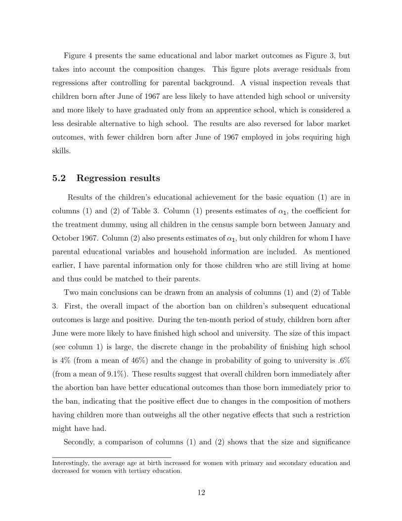
Figure 4 presents the same educational and labor market outcomes as Figure 3, but

takes into account the composition changes. This Þgure plots average residuals from

regressions after controlling for parental background. A visual inspection reveals that

children born after June of 1967 are less likely to have attended high school or university

and more likely to have graduated only from an apprentice school, which is considered a

less desirable alternative to high school. The results are also reversed for labor market

outcomes, with fewer children born after June of 1967 employed in jobs requiring high

skills.

5.2 Regression results

Results of the children�s educational achievement for the basic equation (1) are in

columns (1) and (2) of Table 3. Column (1) presents estimates of α1, the coefficient for

the treatment dummy, using all children in the census sample born between January and

October 1967. Column (2) also presents estimates of α1, but only children for whom I have

parental educational variables and household information are included. As mentioned

earlier, I have parental information only for those children who are still living at home

and thus could be matched to their parents.

Two main conclusions can be drawn from an analysis of columns (1) and (2) of Table

3. First, the overall impact of the abortion ban on children�s subsequent educational

outcomes is large and positive. During the ten-month period of study, children born after

June were more likely to have Þnished high school and university. The size of this impact

(see column 1) is large, the discrete change in the probability of Þnishing high school

is 4% (from a mean of 46%) and the change in probability of going to university is .6%

(from a mean of 9.1%). These results suggest that overall children born immediately after

the abortion ban have better educational outcomes than those born immediately prior to

the ban, indicating that the positive effect due to changes in the composition of mothers

having children more than outweighs all the other negative effects that such a restriction

might have had.

Secondly, a comparison of columns (1) and (2) shows that the size and signiÞcance

Interestingly, the average age at birth increased for women with primary and secondary education anddecreased for women with tertiary education.

12

of the treatment effects for the full and restricted sample are similar. Children still

living with their parents (and for whom I can recover parent background variables) are

on average not affected very differently by the policy compared to the whole population

of children. Thus, I feel comfortable proceeding to the next step of the analysis using

this sub-group to control for the composition of children born into families with different

socio-economic characteristics.

Columns (3) and (4) of Table 3 present the estimates of β1, the coefficient on the treat-

ment dummy after controlling for only the more exogenous background variables (column

3) and both background and household variables from the reduced form equation (2).

This coefficient can be interpreted as the negative unwantedness effect after controlling

for composition effects. As mentioned earlier, this combined unwantedness effect could be

caused by a variety of different theoretically plausible channels, and the present analysis

cannot distinguish between them.

The results in column (4) conÞrm the existence of a large and signiÞcant negative

unwantedness effect. After controlling for family composition, the effect of the abortion

ban on the probability of attending high school or university becomes negative.19 The

results are statistically signiÞcant and substantively large. The change in the probability

of Þnishing high school is -1.7% (from a mean of 51.2%) and the change in probability

of Þnishing university is -1.5% (from a mean of 13.2%). At the same time, the proba-

bility of going to an apprentice school - considered in Romania the default and a less

desirable alternative to high-school - increases by 2.1% (from a mean of 23.2%). Thus,

it appears that, controlling for family background, children born after the introduction

of the abortion ban have worse educational outcomes. As mentioned earlier, I assume

that any unobservable factors that might affect outcomes of children are constant across

individuals. Given the rough control variables available and the fact that composition

and unwantedness have opposite effects in the Romanian case, I believe that if anything

the estimates on the effect of unwantedness are lower bound estimates of the true effect.

As mentioned earlier, one concern with the speciÞcations used in columns (4) is that

some of the controls for the children�s socio-economic background might have been affected

19The reversal of the direction of the association between the abortion ban and child outcomes aftercontrolling for family background is an example of Simpson�s paradox (Simpson, 1951).

13

by the policy change. In particular, the unexpected birth of a child might affect the

household variables (such as square feet per occupant). The regressions in columns (3)

try to correct for this potential source of bias by using only control variables largely

determined at the time of birth: region of birth dummies, urban/rural dummy of birth

for the child, and parents� education.20 Since the results in column (3), which the more

exogenous background variables are generally qualitatively and quantitatively similar to

those in column (4), the discussion of the results will focus primarily on results in column

(4) which include both set of controls.

Table 4 presents the results when conducting the same tests but using labor market

variables instead of educational achievement as outcomes. In the Þrst column I present the

reduced form estimates of equation (1) using the full sample. Similar to the educational

outcomes, the overall effect of the abortion ban on type of employment is positive and

large. The children affected by the policy change were, as adults, less likely to work in

elementary occupations (by -0.6% from a mean of 6.4%) and more likely to work in jobs

requiring a high level of skill (by 0.7% from a mean of 8.6%).

The second column of Table 4 shows estimates from the same regression as in column

(1) but uses the restricted sample. The coefficients are similar to those in the previous

column, although as in the case of the educational outcomes, children living with their

parents have somewhat better outcomes. In columns (3) and (4) I present results from the

estimation of reduced form regression (2), which includes different sets of controls. The

results in column (4) suggest the existence of a negative unwantedness effect in the labor

market. After controlling for family background, the effect of the abortion ban reduces the

probability of working in a high-skill jobs from 9.1% to 8.4% and the change in probability

of working in a job requiring intermediate-skill 1.2% (from a mean of 85.3%).21 The effect

is potentially greater since the census data records employment patterns very early in the

career of the people I study, when there is less variability in outcomes across individuals.

The labor market effect is potentially a lower bound also due to reduced variability in

20Furthermore, the inclusion of different sets of control variables does not affect the basic results. Inall speciÞcations the mother�s education seems to be the most powerful control for family background.

21Additional results not shown here used an alternative deÞnition to create Þve broad occupationaldummy variables, which are broadly reßecting increasing skill in employment: (1) elementary occupations,(2) skilled agriculture, (3) clerical or sales, (4) production, and (5) managers and professionals. The sizeand signiÞcance of these results are similar to those found in the high skill/intermediate skill regressions.

14

employment outcomes resulting from the exclusion of university graduates from the labor

outcome regressions. The use of a later dataset would provide a much better setting for

looking at labor market effects. In particular the currently unreleased 2002 Romanian

census would be a good data source, but by this time we expect very few individuals to

live with their parents.22

5.3 Crowding effects and robustness checks

Table 5 presents the results from the extended framework for schooling outcomes,

including children born in 1965 and 1966, the two years preceding the policy change.

Column (4) of Table 5 conÞrms the existence of large crowding effects in the educational

market. Children born in 1967, who went to school with a cohort that was more than twice

as large as the cohort of the previous year, experience lower educational achievements: the

probability of Þnishing high-school and university decreases by 3.9% and 1.3% respectively,

while the probability of Þnishing only apprentice school increased by 1.7% (from a mean

of 23%). Table 6 suggests that crowding effects in the labor market are small at best.

While the coefficients point in the right direction, they are small and statistically not

signiÞcant.23 The larger crowding effects in schooling outcomes compared to labor market

outcomes are not surprising. The structure of the school system entails that each age

cohort is in a separate grade, so the crowding effects are potentially very large. On the

other hand, the labor market does not have such a tight alignment of jobs to cohorts, so

the crowding effect is spread over the entire labor market in Romania.

The extended framework can also be used to check the robustness of my main Þndings.

The estimates of γ1, the coefficient for the treatment dummy, are broadly similar to the

results from the basic model. If we control for family background, we see that children

22One question of interest concerns the effects in educational and labor market outcomes differ depend-ing on the sex of the child, the urban/rural place of birth, the region of birth of the child and the educationlevels of the parents. In regressions (not reported in the paper), the interaction of these variables withthe treatment dummy were generally small and insigniÞcant. The only exception was the interactionbetween treatment and a female dummy which is positive and signiÞcant in the education regressions.In other words, female children were less likely than male children to suffer the adverse consequences ofthe law.

23The interpretation of the crowding effect in the labor market should be treated with care, since ageeffects might play a signiÞcant role especially at the beginning of the labor market career of individuals.Age effects should be less of a concern for educational outcomes since most people in Romania haveÞnished getting an education by age 25.

15

born after the policy change experience lower educational achievements. While the size of

the magnitude of the probability of Þnishing apprentice school, high school and university

are very similar to those in Table 3, in this speciÞcation the estimate of the high-school

variable is no longer statistically different from 0 at the 5% level. The labor market

outcomes reported in Table 6 are somewhat smaller than my previous Þnding. However,

they generally conÞrm that, once I control for possible compositional and crowding effects,

children born after the ban are less likely to work in high-skill jobs and more likely to

work in intermediate-skill jobs.

Tables 5 and 6 also conÞrm that the effects of being born in the period June 1st

to September 15th are generally very small. Finally, the results of the analysis are not

sensitive to the length of the cohort of birth intervals used, to the inclusion of monthly

time trends or to clustering the standard errors on the treatment dummy.

6 Extensions

6.1 The long-term fertility impact of the policy

This section uses census data from Romania and Hungary to measure the long-term

effect of Romania�s restrictive policies towards abortion and modern contraceptive meth-

ods on fertility levels in general, as well as the differential impact across educational

groups. The magnitude of the long-term fertility impact of this policy is important be-

cause my analysis so far has provided evidence that excess fertility can negatively affect

children�s outcomes. Understanding the long-term effect of the policy across educational

groups is of interest, given that the change in the composition of women who gave birth

had a signiÞcant effect on average child outcomes.

The 1992 Romanian census asked women about the number of children ever born and

thus for women who were over 40 in 1992 (or born prior to 1952) this variable is a good

proxy for lifetime fertility. In Figure 5, I display the average number of children by year

of birth for women born between 1900 and 1955. For women born between 1900 and

1930 I see a gradual and signiÞcant decline in fertility, which is broadly consistent with

the timing of Romania�s rapid demographic transition after World War II. The fertility

impact of the restrictive policy can be observed for women born after 1930. Women born

16

around 1930 were in the their late thirties in 1967 and thus towards the end of their

reproductive years at the time of the policy change. In contrast, the cohorts born around

1950 were in their late teens in 1967 and thus spent basically all their fertile years under

the restrictive regime. The difference in fertility between these two cohorts is large (about

0.4 children or a 25% increase) and is probably a lower bound of the supply side impact

since Romania�s rapid economic development in this period probably decreased demand

for children. Figure 5 also plots the mean number of children born to Hungarians living

in Romania (from the 1992 Romanian census) and to the population in Hungary (from

the 1990 Hungarian census). Hungary and the Hungarian population in Romania provide

good comparison groups, since Hungary did not restrict access to birth control methods.

Figure 5 shows the similar trend in fertility for Hungarians in both countries for women

born prior to 1930 and the divergence in fertility levels afterwards.

Figure 6 presents evidence of increases in the fertility differential between educated and

uneducated women over time. The fertility differential between educated and uneducated

women experienced a gradual decline over time for cohorts born prior to 1930 followed

by a gradual increase for cohorts born afterwards. The differential almost doubled when

cohorts born around 1930 and 1950 are compared.24 Thus the short-run and long-run im-

pacts of the policy were very different between educational groups since educated women

had the largest fertility increases immediately after the introduction of the ban but expe-

rienced the smallest fertility increases during Romania�s 23 year long restrictive policy.25

In a related paper (Pop-Eleches, 2005), I use detailed reproductive microdata26 to pro-

vide an extensive analysis of the fertility impact of the Romanian pronatalist policy. My

results suggest the signiÞcant importance that birth control methods play in inßuencing

fertility levels and the effect of education on fertility.

24The relatively small number of uneducated Hungarians in the Romanian census sample and theinability to properly match educational levels between the Romanian and Hungarian data prevented ananalysis of fertility differentials over time for the Hungarian population.

25This result is complementary to the Þndings of de Walque (2004), who shows the substantial evolutionin the HIV/education gradient during an HIV/AIDS information campaign in Uganda.

26The main dataset used in that paper is the 1993 Romanian Reproductive Health Survey. I am alsousing the 1997 Moldovan Reproductive Health Survey as a control.

17

6.2 Early child outcomes and crime behavior

In this section I explore the effect of the abortion ban on two other socio-economic

variables: early infant outcomes and crime behavior. Figure 7 plots the infant mortality

rate and the late fetal death rate in Romania over the period 1955-1995. The data clearly

suggest that the introduction of the restrictive policy caused large short-term increases

in stillbirths and in infant deaths. Between 1966 and 1968, the infant mortality rate

increased by 27% (from 46.6 to 59.5) and the late fetal death rate increased in the year

following the introduction of the restrictive policy by 22% (from 14.7 to 17.9). Another

indication of the negative impact of the policy change is the similarly large increase in low

birth weights during this period. The percentage of low birth weight children increased

between 1966 and 1967 from 8.1% to 10.6%. These results are consistent with the view

that unwantedness at conception negatively affects early child outcomes. However, these

results could also be explained by reduced access to pre and post-natal care due to possible

crowding in hospitals and health clinics.

Next, following the work of Donohue and Levitt (2001) for the United States, I turn

to the effects of the change in abortion regime on crime behavior later in life. The

crime data27contain all the penal cases in the period 1991-2000 prepared by the regional

tribunal of Sibiu county28 for the regional courts.29 For each of the over 1900 penal cases,

I have basic information about the type of crime committed and most importantly for

my purpose, the year of birth of the persons. I use this information to construct year-age

cells for cohorts born between 1931 and 1985, dividing the number of crimes by the birth

cohort population recorded at the 1992 census. The empirical strategy uses the following

regression framework:

(5) crimeit = θ0 + θ1 · agei + θ2 · yeart + θ3 · born 67 69i + θ4 · born after70i + εi,

where crimeit is a year-age crime rate, agei and yeart are a set of age and year

27Since no government agency collects crime statistics at the individual level for the whole country, thebest alternative was to manually collect data from original archival documents in one region.

28Sibiu, one of Romania�s 42 counties, is located in the center of the country. With a populationof roughly half a million inhabitants, Sibiu is a medium sized county with an above average level ofsocio-economic development.

29In Romania, the regional tribunals with the help of the regional police prepare a detailed report forevery penal crime comitted. This report is then sent to the regional courts who use this evidence todecide the cases.

18

dummies, born 67 69i is an indicator if a cohort was born between 1967 and 1969, the

three years of high fertility. Finally born after70i takes value 1 for cohorts born after

1970.

The basic idea is to look at the crime behavior of cohorts born after the policy change

after accounting for possible age effects and year effects. The cohort of birth indicator

for the period immediately following the introduction of the policy (1967-1969) should

account for the strong compositional changes described earlier, in addition to the nega-

tive unwantedness effect. The effect of the policy change on crime is potentially better

measured for the cohorts born after 1970, a group that is less inßuenced by changes in

the composition of families having children. Column 1 of Table 7 provides regression

results for the total crime rate, which are consistent with my earlier Þndings. The cohort

1967-1969 had an average crime rate30 that was 0.12 lower than the average crime rate of

0.89 for cohorts born prior to 1967. However, cohorts born after 1970 had a 0.3 increase

in their crime rate compared to the cohorts born prior to the policy change. The nega-

tive coefficient for the cohort 1967-1969 suggests that the compositional changes have the

strongest effect on crime behavior, just as in the education and labor regressions. The

positive and signiÞcant coefficient for the cohorts born under the restrictive policy after

1970 provides some suggestive evidence that cohorts born in a period without access to

abortion might experience higher crime rates during adulthood. Since in the medium

and long-run the policy disproportionately affected disadvantaged women (Pop-Eleches,

2002), the increased criminality of cohorts born after 1970 could be explained not just

by changes in the proportion of unwanted children but also by compositional factors.31

However, the present framework cannot control for other time speciÞc factors that might

also have affected the criminal behavior of cohorts born after 1970. As an example, these

results could also be explained by increased criminal behavior of young people during the

transition process.32

30The crime rate equals the number of crimes per 1000 residents in a given birth cohort.31Thus the compositional effect of the ban on abortion for cohorts born after 1970 might have a negative

effect on crime rates, just like in the US after Roe v. Wade (Donohue and Levitt, 2001).32The results in Table 7 are weakened and lose their statistical signiÞcance in speciÞcations that include

age-speciÞc trends.

19

7 Conclusion

This paper has used Romania�s unusual history of abortion legislation to assess the

impact of a change in abortion regime on the socio-economic outcomes of children. On

average, children born after abortion became illegal display better educational and labor

market achievements, and this outcome can be explained by a change in the composition

of families having children: urban, educated women working in good jobs were more

likely to have abortions prior to the policy change, so a higher proportion of children

were born into urban, educated households. Moreover, the analysis shows that after

controlling for this type of compositional changes, the children born after the abortion

ban had signiÞcantly worse schooling and labor market outcomes. I interpret this result

as evidence of the existence of a negative unwantedness effect. The analysis also shows

that crowding in schools, due to the large increase in fertility immediately following the

abortion ban, lowered educational achievements of the cohorts affected. Finally, I have

provided some suggestive evidence consistent with the view that cohorts born after the

introduction of the abortion ban had inferior infant outcomes and increased criminal

behavior later in life.

While the present study has shown evidence of negative developmental effects caused

by a change in abortion policy, the relevance of these Þndings could be of a broader

nature and does not have to refer strictly to abortion legislation. The Þndings of this

study may be relevant in many settings where social, political or economic factors cause

excess fertility, due to lack of access to birth control methods.

20

References

Angrist, J. and Evans, W. (1999), �Schooling and Labor Market Consequences of the

1970 State Abortion Reforms�, Research in Labor Economics, 18, 75-114 .

Becker, G., A Treatise on the Family. Cambridge, MA: Harvard University Press, 1981.

Becker, G. and Lewis, H., �On the Interaction between the Quantity and Quality of

Children�. Journal of Political Economy, 81(2, pt. 2), S279-S288.

Berelson, B. (1979), �Romania�s 1966 Anti-Abortion Decree: The Demographic Expe-

rience of the First Decade�, Population Studies, 33,2, 209-222.

Bloomberg, S (1980), �Inßuence of maternal distress during pregnancy on postnatal

development,� Acta Psychiatrica Scandinavica, 62, 405-417.

Charles, K. and Stephens, M. (2002), �Abortion Legalization and Adolescent Substance

Use�, NBER working paper, no. 9193, Cambrige, MA.

Corman, H. and Grossman, M. (1985), �Determinants of Neonatal Mortality Rates in

the US: A Reduced Form Model,� Journal of Health Economics, 4, 213-236.

David H. P. eds (1999), From Abortion to Contraception, London: Greenwood Press.

David H.P. and Z. Matejcek (1981), �Children Born to Women Denied Abortion: An

Update,� Family Planning Perspectives, 13, 32-34.

David H. P. (1986), �Unwanted Children: A Follow Up from Prague�, Family Planning

Perspectives, 18, 143-144.

de Walque, D. (2004), �How Does the Impact of an HIV/AIDS Information Campaign

Vary with Educational Attainment? Evidence from Rural Uganda�, World Bank Policy

Research Working Paper No. 3289.

Donohue J. J., Grogger, J. and S. D. Levitt (2002), �The Impact of Legalized Abortion

on Teen Childbearing�, University of Chicago mimeo

Donohue J. J. and S. D. Levitt (2001), �The Impact of Legalized Abortion on Crime.�,

Quarterly Journal of Economics, 116(2), 379-420.

21

Dytrych et al.(1975), �Children Born to Women Denied Abortion�, Family Planning

Perspectives, 7, 165-171.

Grossman, M. and Jacobowitz. (1981), �Variations in Infant Mortality Rates Among

Counties of the United States: The Roles of Public Policies and Programs,� Demogra-

phy, 18(4), 695-713.

Goldin, C. and Katz, L. (2002), �The Power of the Pill: Oral Contraceptives and

Women�s Career and Marriage Decisions,� , Journal of Political Economy, 110(4), 730-

770.

Grossman, M. and Joyce, T. (1990), �Unobservables, Pregnancy Resolutions, and Birth

Weight Production Functions in New York City,� Journal of Political Economy, 98(5),

983-1007.

Gruber, J. Levine, P.B. and Staiger, D. (1999), �Abortion Legalization and Child Living

Circumstances: Who is the �Marginal Child?�, Quarterly Journal of Economics, 114(1):

263-291.

Heckman, J. J. (1979), �Sample Selection Bias as a SpeciÞcation Error�, Econometrica,

47(1): 153-161.

Joyce, Th.(1985), �The Impact of Induced Abortion on Birth Outcomes in the United

States.� NBER working paper, no. 1757, Cambrige, MA.

Legge, J. (1985), Abortion Policy: An Evaluation of the Consequences for Maternal

and Infant Health, Albany: State University of New York Press.

Levine, P.B. Staiger, G. Kane, T.J. and Zimmerman, D.J. (1999), �Roe v. Wade and

American Fertility,� American Journal of Public Health, 89(2), 199-203

Pop-Eleches, C. (2005), �The Supply of Birth Control Methods, Education and Fertility:

Evidence from Romania,� Columbia University mimeo

Roy, A. (1951), �Some Thoughts on the Distribution of Earnings,� Oxford Economic

Papers, 3,135-146.

22

Simpson, E.H. (1951), �The Interpretation of Interaction in Contingency Tables�, Jour-

nal of the Royal Statistical Society, Series B, 13: 238-241.

World Bank Country Study. (1992), Romania: Human Resources and the Transition

to a Market Economy. Washington, DC.

World Bank. (1978-1998) World Development Report. New York: Oxford University

Press for the World.

23

FIGURE 1: TOTAL FERTILITY RATES

0

0.5

1

1.5

2

2.5

3

3.5

4

1950 1955 1960 1965 1970 1975 1980 1985 1990 1995 2000YEAR

TFR

Romania

Average (Bulgaria,Hungary, Russia)

Abortion banned

Abortion legalized

Notes: The total fertility rate is the average total number of births that would be born per woman in her lifetime, assuming no mortality in the childbearing ages, calculated from the age distribution and age-specific fertility rates of a specified group in a given reference period. Source: UN (2002).

FIGURE 2: MONTHLY BIRTH RATES - VITAL STATISTICS AND REPRESENTATION INTHE 1992 CENSUS SAMPLE

0

10000

20000

30000

40000

50000

60000

70000

-20 -15 -10 -5 0 5 10 15 20MONTH OF BIRTH (from Jan. 1966 to Dec. 1968)

NU

MB

ER

BO

RN

Monthly Birth Rates

Number of people in census* 7.5

Number of people in censusliving with parents * 15

Notes: This graph plots the number of persons born between 1966 and 1968 by month of birth. Month 0 refers to June 1967, the first month with large fertility increases due to the restrictive abortion policy. Also plotted are the number of persons born in the same period included in the census sample (scaled 1:7.5) and those in the census sample who still lives with their parents (scaled 1:15). Source: 1992 Romanian

FIGURE 3: EDUCATIONAL AND LABOR MARKET ACHIEVEMENTS - RAW DATA

Notes: This graph plots average educational and labor market achievements by month of birth for persons born between 1966 and 1968. Month 0 refers to June 1967, the first month with large fertility increases due to the restrictive abortion policy. Variables are further defined in Appendix A. Source: 1992 Romanian Census.

.15

.22

.3P

erce

nt o

f tot

al

- 1 8 0 18M o n th o f b ir th ( f r o m Ja n . 1 9 6 6 to D e c . 1 9 6 8 )

P a n e l A : A p p re n tic e S c h o o l

.35

.45

.55

Per

cent

of t

otal

- 1 8 0 1 8M o n th o f b ir th ( f r o m Ja n . 1 9 6 6 to D e c . 1 9 6 8 )

P a n e l B : H ig h S c h o o l o r m o re.0

5.1

.15

Per

cent

of t

otal


P a n e l C : U n iv e rs ity o r m o re

.03

.06

.09

Per

cent

of t

otal


P a n e l D : E le m e n ta ry s k ills

.8.8

5.9

Per

cent

of t

otal


P a n e l E : I n te rm e d ia te S k ills

.06

.09

.12

Per

cent

of t

otal


P a n e l F : H ig h S k ills

FIGURE 4: EDUCATIONAL AND LABOR MARKET ACHIEVEMENTS - RESIDUALS AFTER CONTROLLING FOR PARENTAL BACKGROUND

Notes: This graph plots average residuals from educational and labor marker outcome regressions after controlling for parental background by month of birth for persons born between 1966 and 1968. Month 0 refers to June 1967, the first month with large fertility increases due to the restrictive abortion policy. Variables are further defined in Appendix A. Source: 1992 Romanian Census.

-.04

0.0

4P

erce

nt o

f tot

al


P a n e l A : A p p re n t ic e S c h o o l

-.04

0.0

4P

erce

nt o

f tot

al


P a n e l B : H ig h S c h o o l o r m o re-.0

40

.04

Per

cent

of t

otal


P a n e l C : U n iv e rs ity o r m o re

-.04

0.0

4P

erce

nt o

f tot

al


P a n e l D : E le m e n ta ry S k ills

-.04

0.0

4P

erce

nt o

f tot

al


P a n e l E : I n te rm e d ia te S k ills

-.04

0.0

4P

erce

nt o

f tot

al


P a n e l F : H ig h S k ills

FIGURE 5: FERTILITY LEVELS OF WOMEN BORN BETWEEN 1900-1955

1

1.5

2

2.5

3

1915 1920 1925 1930 1935 1940 1945 1950 1955

YEAR OF BIRTH

CH

ILD

RE

N E

VE

R B

OR

N (M

EA

N)

Romania overall Hungarians in Romania overall Hungary overall

Notes: This graph plots the average number of children born in Romania by year of birth of the mother. Similar data is shown for the Hungarian minority in Romania and for Hungary. Hungary did not implement a similar restriction during this time period. Source: 1992 Romanian Census, 1990 Hungarian Census.

FIGURE 6: FERTILITY LEVELS IN ROMANIA BY EDUCATION

0

0.5

1

1.5

2

2.5

3

3.5

4

1915 1920 1925 1930 1935 1940 1945 1950 1955YEAR OF BIRTH

CH

ILD

REN

EV

ER B

OR

N (M

EAN

)

Uneducated Educated Differential (Uneducated-Educated)

Notes: This graph plots the average number of children born by year of birth of the mother and educational level. Source: 1992 Romanian Census.

FIGURE 7: INFANT MORTASLITY RATE, LATE FETAL DEATH RATE, AND LOW BIRTH WEIGHT RATE IN ROMANIA (1955-1995)

0

10

20

30

40

50

60

70

80

1955 1960 1965 1970 1975 1980 1985 1990 1995YEAR

INFA

NT

MO

RT

AL

ITY

AN

D L

AT

E F

ET

AL

DE

AT

H R

AT

E

0

0.02

0.04

0.06

0.08

0.1

0.12

LO

W B

IRT

H W

EIG

HT infant mortality rate

late fetal death rate

low birth weight

Notes: This graph plots the infant mortality rate, the late fetal death rate and the low birth weight rate for Romania in the period 1955-1995. Source: Government of Romania, Statistical Office.

Table 1: Summary statistics

Full Sample Do not live Restricted sample Full Sample Full Sample Restricted Sample Restricted SampleDependent Variables with either (Live with Diff. Controls Treatments Diff. Controls Treatments Diff.

(Jan.-Oct. 1967) parent both parents) (Jan.-May 1967) (June-Oct.1967) (Jan.-May 1967) (June-Oct.1967)

Female 0.481 0.626 0.331 -0.295*** 0.474 0.484 0.009** 0.313 0.339 0.026***

Urban 0.397 0.347 0.436 0.089*** 0.350 0.421 0.072*** 0.374 0.464 0.089***

Apprentice School 0.226 0.222 0.232 0.001*** 0.222 0.228 0.006* 0.231 0.233 0.0020.460 0.420 0.512 0.092*** 0.435 0.472 0.038*** 0.484 0.525 0.041***

University or more 0.091 0.058 0.132 0.074*** 0.087 0.093 0.006** 0.127 0.133 0.006

0.064 0.068 0.056 -0.012*** 0.068 0.061 -0.006** 0.060 0.054 -0.006*0.850 0.849 0.853 0.004 0.851 0.850 -0.001 0.852 0.854 0.002

High Skills 0.086 0.083 0.091 0.008*** 0.081 0.089 0.007*** 0.088 0.092 0.004

Observations 55337 27417 22847 18339 36998 7147 15700Obs. for Job Type 41898 20648 17335 13840 28058 5416 11919

Notes: The full sample contains people born between January and October of 1967. The restricted sample contains children living with both their parents at the time of the census in 1992, for whom I could obtain basic socio-economic variables of their parents. The persons born between January and May of 1967 are in the control group, while those born between June and October are in the treatment group. * indicates statistical significance at the 10% level, ** at 5% and *** at 1% for the difference in means.Variables are further defined in Appendix A.

Child's Job Type

Elementary SkillsIntermediate Skills

Gender of Child

Place of Birth

Child's Education

High School or more

Table 2: Selection effects of the change in abortion legislation: comparison of means

Control Group Treatment Group (Jan.-May 1967) (June-October 1967) Difference

Urban 0.350 0.422 0.071***

Observations 19156 38494

Primary 0.494 0.446 -0.048***

Secondary 0.476 0.521 0.045***

Tertiary 0.030 0.033 0.003


Primary 0.370 0.323 -0.047***

Secondary 0.576 0.613 0.038***

Tertiary 0.055 0.064 0.009***Observations 7574 16601

Primary 29.188 29.497 0.309***

Secondary 25.874 26.452 0.578***

Tertiary 28.743 27.969 -0.774**


Notes: The sample contains parents who had children born between January and October of 1967and living at home at thetime of the census in 1992. The Control Group contains people born between January and May 1967. The Treatment Groupcontains people born between June - October 1967. * indicates statistical significance at the 10% level, ** at 5% and *** at1% for the difference in means. Variables are further defined in Appendix A.

Place of Birth of Child

Mother's Highest Educational Level

Mother's Age at Birth by Education

Father's Highest Educational Level

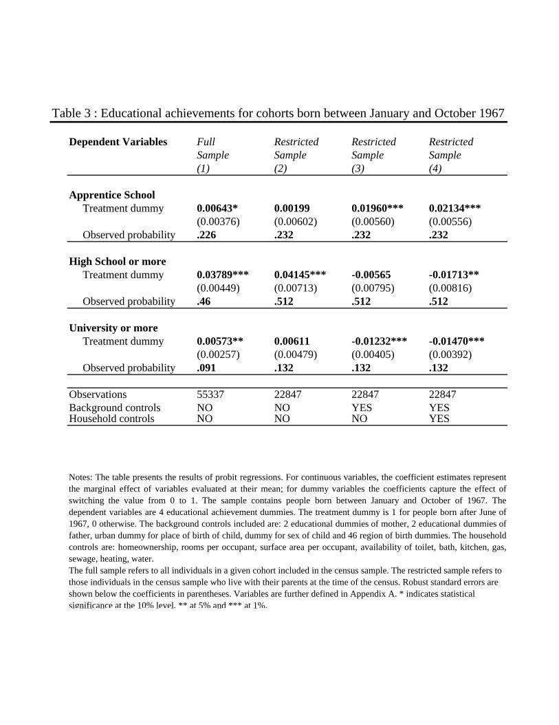
Table 3 : Educational achievements for cohorts born between January and October 1967

Dependent Variables Full Restricted Restricted RestrictedSample Sample Sample Sample(1) (2) (3) (4)

Apprentice School Treatment dummy 0.00643* 0.00199 0.01960*** 0.02134***

(0.00376) (0.00602) (0.00560) (0.00556) Observed probability .226 .232 .232 .232

High School or more Treatment dummy 0.03789*** 0.04145*** -0.00565 -0.01713**


University or more Treatment dummy 0.00573** 0.00611 -0.01232*** -0.01470***


Observations 55337 22847 22847 22847Background controls NO NO YES YESHousehold controls NO NO NO YES

Notes: The table presents the results of probit regressions. For continuous variables, the coefficient estimates representthe marginal effect of variables evaluated at their mean; for dummy variables the coefficients capture the effect ofswitching the value from 0 to 1. The sample contains people born between January and October of 1967. Thedependent variables are 4 educational achievement dummies. The treatment dummy is 1 for people born after June of1967, 0 otherwise. The background controls included are: 2 educational dummies of mother, 2 educational dummies offather, urban dummy for place of birth of child, dummy for sex of child and 46 region of birth dummies. The householdcontrols are: homeownership, rooms per occupant, surface area per occupant, availability of toilet, bath, kitchen, gas,sewage, heating, water. The full sample refers to all individuals in a given cohort included in the census sample. The restricted sample refers to those individuals in the census sample who live with their parents at the time of the census. Robust standard errors are shown below the coefficients in parentheses. Variables are further defined in Appendix A. * indicates statistical significance at the 10% level, ** at 5% and *** at 1%.

Table 4 : Labor market outcomes for cohorts born between January and October 1967

Dependent Variables Full Restricted Restricted RestrictedSample Sample Sample Sample(1) (2) (3) (4)

Elementary Skills Treatment dummy -0.00644** -0.00608 -0.00287 -0.00167


Intermediate Skills Treatment dummy -0.00098 0.00186 0.01214** 0.01241**


High Skills Treatment dummy 0.00742*** 0.00422 -0.00639 -0.00729*


Observations 41898 17335 17335 17335Background controls NO NO YES YESHousehold controls NO NO NO YES

Notes: The table presents the results of probit regressions. For continuous variables, the coefficient estimates representthe marginal effect of variables evaluated at their mean; for dummy variables the coefficients capture the effect ofswitching the value from 0 to 1. The sample contains people born between January and October of 1967. Thedependent variables are 3 skill specialization dummies based ISCO 88 occupational codes. The treatment dummy is 1for people born after June of 1967, 0 otherwise. The background controls included are: 2 educational dummies ofmother, 2 educational dummies of father, urban dummy for place of birth of child, dummy for sex of child and 46region of birth dummies. The household controls are: homeownership, rooms per occupant, surface area per occupant,availability of toilet, bath, kitchen, gas, sewage, heating, water.The full sample refers to all individuals in a given cohort included in the census sample. The restricted sample refers to those individuals in the census sample who live with their parents at the time of the census. Robust standard errors are shown below the coefficients in parentheses. Variables are further defined in Appendix A. * indicates statistical significance at the 10% level, ** at 5% and *** at 1%.

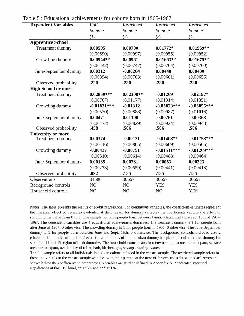
Table 5 : Educational achievements for cohorts born in 1965-1967Dependent Variables Full Restricted Restricted Restricted

Sample Sample Sample Sample(1) (2) (3) (4)

Apprentice School Treatment dummy 0.00595 0.00700 0.01772* 0.01969**

(0.00590) (0.00997) (0.00955) (0.00952) Crowding dummy 0.00944** 0.00961 0.01663** 0.01675**

(0.00442) (0.00747) (0.00704) (0.00700) June-September dummy 0.00312 -0.00264 0.00448 0.00430

(0.00394) (0.00703) (0.00661) (0.00656) Observed probability .220 .230 .230 .230High School or more Treatment dummy 0.02869*** 0.02308** -0.01269 -0.02197*

(0.00707) (0.01177) (0.01314) (0.01351) Crowding dummy -0.01831*** -0.01312 -0.03823*** -0.03855***

(0.00530) (0.00888) (0.00987) (0.01016) June-September dummy 0.00471 0.01100 -0.00261 -0.00363

(0.00472) (0.00829) (0.00924) (0.00948) Observed probability .458 .506 .506 .506University or more Treatment dummy 0.00374 -0.00131 -0.01408** -0.01758***

(0.00416) (0.00805) (0.00609) (0.00565) Crowding dummy -0.00437 -0.00751 -0.01511*** -0.01269***

(0.00310) (0.00614) (0.00488) (0.00464) June-September dummy 0.00185 0.00781 0.00053 0.00223

(0.00273) (0.00559) (0.00441) (0.00413) Observed probability .092 .135 .135 .135Observations 84508 30657 30657 30657Background controls NO NO YES YESHousehold controls NO NO NO YES

Notes: The table presents the results of probit regressions. For continuous variables, the coefficient estimates representthe marginal effect of variables evaluated at their mean; for dummy variables the coefficients capture the effect ofswitching the value from 0 to 1. The sample contains people born between January-April and June-Sept.15th of 1965-1967. The dependent variables are 4 educational achievement dummies. The treatment dummy is 1 for people bornafter June of 1967, 0 otherwise. The crowding dummy is 1 for people born in 1967, 0 otherwise. The June-Septemberdummy is 1 for people born between June and Sept. 15th, 0 otherwise. The background controls included are: 2educational dummies of mother, 2 educational dummies of father, urban dummy for place of birth of child, dummy forsex of child and 46 region of birth dummies. The household controls are: homeownership, rooms per occupant, surfacearea per occupant, availability of toilet, bath, kitchen, gas, sewage, heating, water. The full sample refers to all individuals in a given cohort included in the census sample. The restricted sample refers to those individuals in the census sample who live with their parents at the time of the census. Robust standard errors are shown below the coefficients in parentheses. Variables are further defined in Appendix A. * indicates statistical significance at the 10% level, ** at 5% and *** at 1%.

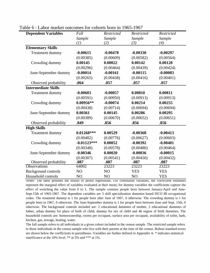
Table 6 : Labor market outcomes for cohorts born in 1965-1967Dependent Variables Full Restricted Restricted Restricted

Sample Sample Sample Sample(1) (2) (3) (4)

Elementary Skills Treatment dummy -0.00615 -0.00478 -0.00330 -0.00297

(0.00385) (0.00609) (0.00582) (0.00564) Crowding dummy 0.00145 0.00022 0.00142 0.00128

(0.00296) (0.00464) (0.00439) (0.00424) June-September dummy -0.00014 -0.00161 -0.00115 -0.00083

(0.00265) (0.00438) (0.00416) (0.00401) Observed probability .064 .057 .057 .057Intermediate Skills Treatment dummy -0.00603 -0.00057 0.00810 0.00811

(0.00591) (0.00950) (0.00913) (0.00913) Crowding dummy 0.00956** -0.00074 0.00214 0.00255

(0.00438) (0.00714) (0.00694) (0.00694) June-September dummy 0.00361 0.00145 0.00286 0.00295

(0.00389) (0.00670) (0.00652) (0.00651) Observed probability .849 .856 .856 .856High Skills Treatment dummy 0.01268*** 0.00529 -0.00368 -0.00413

(0.00482) (0.00776) (0.00627) (0.00603) Crowding dummy -0.01123*** 0.00052 -0.00392 -0.00401

(0.00348) (0.00578) (0.00480) (0.00464) June-September dummy -0.00346 0.00020 -0.00036 -0.00015

(0.00307) (0.00541) (0.00450) (0.00432) Observed probability .087 .087 .087 .087Observations 64002 23223 23223 23223Background controls NO NO YES YESHousehold controls NO NO NO YESNotes: The table presents the results of probit regressions. For continuous variables, the coefficient estimatesrepresent the marginal effect of variables evaluated at their mean; for dummy variables the coefficients capture theeffect of switching the value from 0 to 1. The sample contains people born between January-April and June-Sept.15th of 1965-1967. The dependent variables are 3 skill specialization dummies based ISCO 88 occupationalcodes. The treatment dummy is 1 for people born after June of 1967, 0 otherwise. The crowding dummy is 1 forpeople born in 1967, 0 otherwise. The June-September dummy is 1 for people born between June and Sept. 15th, 0otherwise. The background controls included are: 2 educational dummies of mother, 2 educational dummies offather, urban dummy for place of birth of child, dummy for sex of child and 46 region of birth dummies. Thehousehold controls are: homeownership, rooms per occupant, surface area per occupant, availability of toilet, bath,kitchen, gas, sewage, heating, water. The full sample refers to all individuals in a given cohort included in the census sample. The restricted sample refers to those individuals in the census sample who live with their parents at the time of the census. Robust standard errors are shown below the coefficients in parentheses. Variables are further defined in Appendix A. * indicates statistical significance at the 10% level, ** at 5% and *** at 1%.

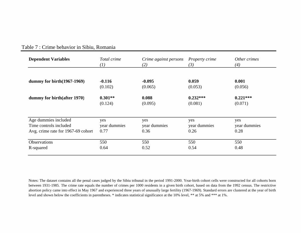
Table 7 : Crime behavior in Sibiu, Romania

Dependent Variables Total crime Crime against persons Property crime Other crimes(1) (2) (3) (4)

dummy for birth(1967-1969) -0.116 -0.095 0.059 0.001(0.102) (0.065) (0.053) (0.056)

dummy for birth(after 1970) 0.301** 0.088 0.232*** 0.221***(0.124) (0.095) (0.081) (0.071)

Age dummies included yes yes yes yesTime controls included year dummies year dummies year dummies year dummiesAvg. crime rate for 1967-69 cohort 0.77 0.36 0.26 0.28

Observations 550 550 550 550R-squared 0.64 0.52 0.54 0.48

Notes: The dataset contains all the penal cases judged by the Sibiu tribunal in the period 1991-2000. Year-birth cohort cells were constructed for all cohorts bornbetween 1931-1985. The crime rate equals the number of crimes per 1000 residents in a given birth cohort, based on data from the 1992 census. The restrictiveabortion policy came into effect in May 1967 and experienced three years of unusually large fertility (1967-1969). Standard errors are clustered at the year of birthlevel and shown below the coefficients in parentheses. * indicates statistical significance at the 10% level, ** at 5% and *** at 1%.

Appendix A: Definition of the variables

This table describes the variables from the 1992 Romanian census used in this study.

1. Dependent variables:

Educational achievements:

Romania’s educational system is organized as follows: after 8 years of primary school, which virtually all children attend, a student has the choice to go to high-school for four years or to go to an apprentice school. The apprentice schools, which resemble the vocational schools in other European countries, are also 4 years long and they combine formal schooling with on job practical training but do not allow a student to apply for a university degree. Only graduates of high-schools are allowed to apply to universities. Definition of education variables:

Apprentice School – this variable takes value 1 if an individual has graduated from an apprentice school, 0 otherwise

High School or more– this variable takes value 1 if an individual has graduated from high school, 0 otherwise. Thus, this variable includes those individuals who received tertiary education

University or more – this variable takes value 1 if an individual has graduated from university or a postgraduate school or is currently enrolled in university, 0 otherwise. Current enrollment in university is defined as having a high school degree and being currently in enrolled in school.

Labor market outcomes:

The labor market outcomes refer to those individuals currently employed in one of the four major ISCO skill Groups. The ISCO (International Standard Classification of Occupations) codes classify jobs with respect to the type of work performed and the skill level required to carry out the tasks and duties of the occupations. The ISCO is the standard classification of the International Labor Organization (ILO). Since a sizeable fraction of individuals were still enrolled in university at the time of the survey, individuals with a university degree or those currently enrolled in university were dropped from the labor market regressions. Definition of labor market variables:

Elementary skills– this variable takes value 1 if an individual is employed at the time of the census in an ISCO skill level 1 occupation, 0 if employed in a different skill level occupation.

Intermediate skills– this variable takes value 1 if an individual is employed at the time of the census in an ISCO skill level 2 occupation, 0 if employed in a different skill level occupation.

High skills– this variable takes value 1 if an individual is employed at the time of the census in an ISCO skill level 3 or 4 occupation, 0 if employed in a different skill level occupation.

2. Independent variables:

Educational achievements of parents:

Secondary Education – this variable takes value 1 if an individual has graduated from secondary school (either high school or apprentice school), 0 otherwise.

Tertiary Education – this variable takes value 1 if an individual has tertiary education , 0 otherwise.

Household variables (refer to endowment of household at the time of the census in 1992): Homeownership – this variable takes value 1 if a household owns the home where it lives at the time of the

census, 0 otherwise. Rooms per occupant– this variable measures the number of rooms in the household per number of

household members at the time of the census. Surface area per occupant– this variable measures the surface area (measured in square meters) in the

household per number of household members at the time of the census.

Toilet – this variable takes value 2 if a household has a toilet inside the dwelling unit, 1 if a household has a toilet outside the dwelling unit, 0 if a household has no toilet

Bath– this variable takes value 2 if a household has a bath inside the dwelling unit, 1 if a household has a bath outside the dwelling unit, 0 if a household has no bath.

Kitchen– this variable takes value 2 if a household has a kitchen inside the dwelling unit, 1 if a household has a kitchen outside the dwelling unit, 0 if a household has no kitchen.

Gas– this variable takes value 1 if a household has access to gas for cooking in the household, 0 otherwise Sewage– this variable takes value 1 if a household is connected to a sewerage system, 0 otherwise Heating– this variable takes value 1 if a household has central heating in the household, 0 otherwise Water– this variable takes value 1 if a household has access to hot water in the household, 0 otherwise

Other variables:

Urban – this variable takes value 1 if an individual was born in a urban area, 0 otherwise. Sex– this variable takes value 1 if an individual is female, 0 otherwise. Region of birth– these are a set of 47 region of birth dummies. Fertility – the number of live births born to a female respondent at the time of the 1992 census

The Impact of an Abortion Ban on Socio-Economic …cp2124/papers/unwanted_latest.pdfThe Impact of an...

Documents

Transcript of The Impact of an Abortion Ban on Socio-Economic …cp2124/papers/unwanted_latest.pdfThe Impact of an...