The Impact of Aggregate Changes in Fundamental Analysis on ...
48
The Impact of Aggregate Changes in Fundamental Analysis on Macroeconomic Forecasts Master Thesis Hans Bresser, 32342 Finance Double Degree Program Supervisor: Maria João Major Nova School of Business and Economics Date: 11.12.2018
Transcript of The Impact of Aggregate Changes in Fundamental Analysis on ...

The Impact of Aggregate Changes in Fundamental
Analysis on Macroeconomic Forecasts
Master Thesis
Hans Bresser, 32342
Finance
Double Degree Program
Supervisor: Maria João Major
Nova School of Business and Economics
Date: 11.12.2018

1
1. Introduction
Macroeconomic forecasts are crucial for the well-being of the economy as they provide
stakeholders with information on the macro as well as micro level to optimise resource allocation,
minimise waste and ensure a stable business environment. Thus, this thesis attempts to use
aggregate accounting information to contribute to the enhancement of macroeconomic forecasts.
Several potential user groups for macroeconomic forecasts exists. Central banks intend to
foresee future developments of the economy to set a desired level of inflation by lowering (raising)
interest rates to incentivise (discentivise) investors during recessions (upswings) to keep the
economy close to equilibrium (Carlin & Soskice, 2015). Individuals and entrepreneurs intend to
benefit from booms or reduce their downside risk. Beyond, employers utilise forecasts to set
benchmarks for wage setting purposes and business planners must be informed about the current
stage of the business cycle to evaluate the sustainability of existing or new product lines (Carlin
& Soskice, 2015). Therefore, it is crucial to continuously refine macroeconomic forecast models.
Konchitchki and Patatoukas (2014) started the ball rolling by investigating the usefulness
of aggregate accounting data on macroeconomic forecasting and find financial performance ratios
to contain predictive power for subsequent macroeconomic growth. Their idea is intended to be
further developed and tested by highlighting the usefulness of the F-Score (Piotroski, 2000), a
financial performance metric created to assess firms’ financial fundamentals. The F-Score is
composed of so-called binary signals that sum up to a final score. Hence, aggregate changes in
Total F-Score, as well as its components (Partial F-Scores), serve as explanatory variables to
predict subsequent macroeconomic growth.
As the name suggests, macroeconomic forecasts are forward looking, a characteristic necessary
for being valuable. For example, when regarding monetary policy, the economy displays a lagged
reaction of at least six months with the consequence that macroeconomic forecasts, as well as
monetary policy, must be forward looking to compensate for the delayed response in the economy

2
(Carlin & Soskice, 2015). Nevertheless, this characteristic comes at the cost of imprecision, as
even the most thorough analysis and forecast is incapable to perfectly predict the future. This
inevitable imprecision leads to at least partially faulty resource allocation and thus to an overall
loss to the economy. To minimise this imprecision and its associated costs, macroeconomists
attempt to improve forecasting models and conceive new ideas to reduce forecasting errors. One
such attempt is the research conducted by Konchitchki and Patatoukas (2014), who investigate a
relatively unexplored approach by utilising financial statement analysis for macroeconomic
predictions and analyse the extent to which the Survey of Professional Forecasters (SPF) by the
Federal Reserve Bank of Philadelphia, incorporates this type of information.
Financial statement analysis summarises the economic consequences of a company’s business
activities. Accounting standards such as the US GAAP intend to provide a framework for
companies to deal with the trade-off between overly loose and overly tight regulations. These
standards limit the company’s ability to inaccurately represent their financial position and
facilitate comparisons between various firms (Kieso, Weygandt & Warfield, 2014; Palepu, Healy
& Peak, 2016). Furthermore, companies’ financial positions appear to be persistent over time,
making them predictable and therefore valuable as incremental information for macroeconomic
projections (Soliman, 2008). Konchitchki and Patatoukas (2014), advertise the usefulness of
aggregate accounting data of the largest corporations in the United States (US). Their study makes
use of the fact that listed firms represent a large part of the US economy, and thus changes in their
financials are informative for overall economic activity. This simplicity and thus its low-cost
characteristics is the most significant strength of their methodology, as only a small number of
firms must be analysed.
Building up on this research, this thesis attempts to further illuminate the usefulness of financial
statement and fundamental analysis on macroeconomic forecasts by assessing the explanatory
power of the F-Score. The F-Score assesses three areas of a company’s financial position:

3
profitability, financial liquidity/leverage and operational efficiency. Detailed descriptions about
the composition of the F-Score are provided in the literature review.
Combining fundamental analysis with macroeconomic forecasting is a new field of study.
Konchitchki and Patatoukas (2014) abandon the idea of using aggregate accounting information
solely on the firm level but attempt to make use of macroeconomic predictive characteristics of
aggregated financial statement analysis of influential firms. Moreover, this idea fills a void in the
literature in terms of evaluating SPF forecast errors. While much prior literature deals with
improvements related to econometric models (Bratu, 2012; Croushore, 2010), the concept of
Konchitchki and Patatoukas (2014) considers the heretofore disregarded usefulness of aggregate
accounting data. Also, Kalay, Nallareddy & Sadka (2018) pick up on their research, to
demonstrate the explaining power of firm-level shocks on macroeconomic shocks. The intention
of this study is to further widen the perspective and assess the predictive power of fundamental
analysis, proxied by the F-Score, on macroeconomic forecasts.
In the following subsection the evolution of the usefulness of financial statement data is discussed.
Section 3 addresses the utilised data sources and applied methodology. Section 4 presents the
results of the proposed models, including statistical interpretation and economical intuition.
Section 5 concludes the study by addressing the main findings and acknowledging about
limitations of the study and presenting concerns for future research.
2. Literature Review
2.1 Evolution of the Utilisation of Accounting Earnings Data
Konchitchki and Patatoukas (2014) shift the focus of the predictive power of financial statement
analysis from the micro to the macro level. Therefore, the following section serves as quick
orientation of the evolution of financial statement analysis and the use of its predictive power.
In the late 1980s, Ou and Penman (1989) propose a strategy for yielding abnormal returns
based on financial statement analysis. The basic idea is to invest in firms that show strong

4
fundamentals and thus benefit from imperfect financial markets, as these fundamental measures
are not fully incorporated in current stock prices, which leads to the undervaluation
(overvaluation) of equity values with strong (weak) fundamentals. This discovery can be
considered as first indicator that accounting data contain leading information for subsequent
periods and thus be the starting point for this study. This research is further refined by Abarbanell
and Bushee (1998) by considering the grouped variables in isolation and adding causal reasoning
to the statistical relationships. The methodology is developed even further when Soliman (2008)
researches the persistence of financial ratios by utilising the so-called DuPont analysis which
decomposes return on net operating assets (RNOA), into the two-profitability driver asset turnover
(ATO) and profit margin (PM). Decomposed into the DuPont profitability ratio, the variables
demonstrate persistence and therefore the potential to possess predictive power for subsequent
periods. Lately, the American Accounting Association has built up on research conducted by
Dechow (1994) who demonstrates that accrual earnings are more advanced for measuring firm
performance in the short term than actual cash flows, suggesting that accounting earnings data
possess much better predictive power for subsequent cash flows than cash flows of the current
period (Moehrle et al., 2009). By following the wide-spread assumption that firm value is equal
to the present value of companies’ future cash-flows (Berk & DeMarzo, 2014), the use of
accounting data can lead improvements for firm valuation and economic projections in general.
Following these mostly incremental changes in the utilisation of accounting earnings data
Konchitchki and Patatoukas (2014) introduce a game changing idea that utilises the predictive
power of aggregate accounting data on the macro instead of micro level. The academics focus on
the 100 most influential firms ranked by market capitalisation in the US, which are responsible
for about 80% of the country’s economic activity and therefore provide a reasonable and cost-
effective method to proxy the real economy. Their results show that aggregate accounting data
contain predictive power for macroeconomic projections and professional forecasters partially

5
revise their projections of real economic activity according to recently published aggregate
accounting data. However, they are not as fully attuned to aggregate accounting data as to stock
market data leaving room for improvement. As the classic DuPont breakdown, as well as further
refinements of this breakdown are the focus of the latest literature stream and serve as the
foundation for this study, they are explained in detail in the following section.
2.2 Breakdowns
In the backbone paper of this study, Konchitchki and Patatoukas (2014) assess firm performance
by measuring RNOA and decomposing it into the DuPont profitability ratio which is composed
of two parts: ATO, measured by volume of sales over net operating assets and PM, which is
calculated by operating income after depreciation over volume of sales. The former measures
firms’ asset utilisation, or how efficiently assets are used to generate sales and consequently the
extent to which firms are able to materialise on their assets. The latter measures firms’ operating
efficiency by revealing how much money firms generate per dollar of sales and their ability to
control costs and charge premium prices (Fairfield & Yohn, 2001). Thus, the DuPont profitability
ratio provides insights about the drivers of firms’ operating profitability and demonstrates firms’
value creation potential, as it is based on unlevered financial statements and unbiased by any
financing decisions (Baumann, 2014). They find that RNOA is a significant predictor for
subsequent GDP growth, which is mainly driven by the predictive power of PM.
Ivanov (2016) argues that the classic DuPont breakdown does not represent the optimal
breakdown for the purpose of macroeconomic forecasting. Thus, he introduces the alternative
DuPont breakdown, which incorporates the effect of financial leverage:
𝑅𝑂𝐸 = 𝑅𝑂𝐵𝐴 + (𝑅𝑂𝐵𝐴 − 𝐴𝑓𝑡𝑒𝑟 𝑡𝑎𝑥 𝐶𝑜𝑠𝑡 𝑜𝑓 𝐷𝑒𝑏𝑡) × 𝐹𝑖𝑛𝑎𝑛𝑐𝑖𝑎𝑙 𝐿𝑒𝑣𝑒𝑟𝑎𝑔𝑒
Spread
The central difference to the classic DuPont breakdown is that ROE, rather than RNOA, is
decomposed. Return on business assets (ROBA) measures the profitability from the company’s

6
operating and investment activities. The spread is calculated as the difference between ROBA and
the after-tax cost of debt. It infers the crucial importance that a company earns more than the
invested funds cost as otherwise, the company destructs, rather than creates value for both
shareholder and debtholder. Hence, if firms manage to earn a higher return than their cost of debt,
they have the potential to grow, which in turn can be an indicator for macroeconomic growth.
Ivanov (2016) finds that the spread component is a powerful predictor for subsequent
macroeconomic activity and thus proves that a levered perspective on firm performance provides
valuable information for macroeconomic forecasting.
F-Score (Total_FScore)
As this study attempts to further simplify the methodology, the F-Score is utilised to benefit from
its easily understandable binary nature. The F-Score is a financial performance metric that aims
to assess firms’ fundamentals according to nine binary financial performance signals. It is first
introduced by Piotroski in 2000, who attempts to assess firms’ financial health to foresee price-
adjusting effects. Consequently, firms with weak (strong) fundamentals are on average overvalued
(undervalued). Thus, investors can earn abnormal profits by investing (divesting) in undervalued
(overvalued) stocks and hence exploiting market inefficiencies (Piotroski, 2000; Piotroski & So,
2012). However, the proposed simplicity comes at a cost. Relevant factors may not be considered
in the assessment due to its binary nature which can lead to biased outcomes. Nevertheless,
Piotroski (2000) and Piotroski and So (2012), show that the F-Score leads to significant results
and implications for firms’ current financial positions and contains information about firm’s next
period’s financial strength. To test the extent to which quarterly aggregate changes in Total F-
Scores provide insights for forecasting, the first hypothesis is proposed:
Hypothesis 1: Quarterly aggregate changes in Total F-Scores contain predictive power for
subsequent macroeconomic growth.

7
The composition of the F-Score can be grouped into three so-called Partial F-Scores, which are
assigned to the following areas: profitability, liquidity/leverage and operational efficiency. Hence,
the second hypothesis refers to the overall predictive power of the three Partial F-Scores:
Hypothesis 2: Quarterly aggregate changes in Partial F-Scores contain predictive power for
subsequent macroeconomic growth.
Current profitability and cash collection provide information about a company’s ability to
generate funds internally. Any enterprise experiencing a positive cash flow or earning profits can
demonstrate that it is capable of generating funds from operating activities. Moreover, increasing
earnings is an accurate predictor of a company’s future ability to generate positive cash flows.
However, earnings that are primarily driven by positive accrual accounting adjustments are a bad
signal for future profitability. Having excessive positive accrual accounting adjustments indicates
that earnings exceed cash flow from operations (CFO), this is in turn, an indicator that the
company is unable to collect cash and realise its returns. (Piotroski, 2000; Sloan, 1996). Piotroski
(2000) defines four variables in order to assess firms’ profitability: ROA (BS1_ROA), change in
ROA (BS2_ROA), CFO (BS3_CFO) and current year’s net income before extraordinary items
less CFO (BS4_Accrual). The predictive power of the profitability Partial F-Score is consequently
tested, which leads to the following hypothesis:
Hypothesis 2.1: Quarterly aggregate changes in the profitability Partial F-Scores show power
for subsequent macroeconomic growth
The second area of financial performance signals refers to a company’s ability to meet future (debt
service) obligations. Piotroski (2000) assumes that an increase in leverage, a lack of current assets
and the reliance on external funding are signals for weak financial fundamentals. Therefore, he
introduces three variables related to debt obligations and liquidity issues: Change in a firm’s long-
term debt levels (BS5_Debt), change in a firm’s current ratio (BS6_currentratio), Equity Issuance
(BS7_Equity). Overall, the liquidity and leverage Partial F-Score indicates a firm’s ability to yield

8
a higher return than the used cost of capital and thus provides insights into the well-being of a
company, since a successful and sustainable firm does not only rely on overall profitability but is
also required to pay back it’s debtholders (Piotroski, 2000). Therefore, whether the predictive
power of financial liquidity/ on macroeconomic forecasts is investigated:
Hypothesis 2.2: Quarterly aggregate changes in the liquidity and leverage Partial F-Score show
predictive power for subsequent macroeconomic growth.
As final area for firms’ financial health, operational efficiency is assessed. Therefore, the two
components of the classic DuPont breakdown, the decomposition of ROA into ATO (BS8_ATO)
and PM (BS9_PM), are tested for their implications for macroeconomic forecasting:
Hypothesis 2.3: Quarterly aggregate changes in the operational efficiency Partial F-Score show
predictive power for subsequent macroeconomic growth.
2.4 The Stock Market as Benchmark Model for publicly available Information
Macroeconomic predictions based on aggregate accounting data are only relevant for future
research if they do not overlap with information that is already used by the public. Therefore, an
easily available benchmark model must be chosen to examine whether variables demonstrate
incrementally useful value in addition to information that is already captured by the market.
According to the efficient market hypothesis, the stock market reflects timely information about
the current well-being and consequently also about the future outlook of the economy.
Consequently, the stock market can be considered as leading indicator for future changes in
macroeconomic growth. (Fama, 1990; Fama & French, 1992). The most famous and broad-based
stock market index for the US economy is the S&P 500 index, it includes the most valuable
companies in the United States which are listed on the NYSE or NASDAQ stock market
exchanges. The S&P 500 differs from other popular US stock indexes, such as the Dow Jones
Industrial Average or the NASDAQ composite index, as the incorporated companies are much
more diverse and therefore provide a useful solution to proxy the entire economy (Berk &

9
DeMarzo,2014). Consequently, fluctuations do not depend excessively on distinct industries but
reflect a broad-based set of companies from various areas and hence serves as a good proxy for
the entire US economy. Consequently, it is tested for the extent to which the findings are
incrementally useful to information that is already incorporated in the stock market:
Hypothesis 3: Adjusting models for predicting macroeconomic growth (GDP) by adding insights
from financial statement analysis adds incremental value and does not coincide with already
available information in the market, proxied by the S&P 500 stock market index.
2.5 Proxy for the Real Economy
The key strength of the research design of Konchitchki and Patatoukas (2014) is its simplicity and
cost efficiency, because only the 100 most influential firms need to be analysed in order to create
a reasonable proxy for the real economy. The top 100 account for roughly 82% of the overall
market capitalisation and show that the correlation between aggregate changes in accounting
profitability (proxied by RNOA) of the 100 largest firms and all firms is 0.99.
The researchers use firms’ market value (MV) to determine their relative size and thus rank the
corporations. Using MV as ranking method leads to potential drawbacks. Firstly, stocks are
publicly traded and reflect high volatility. Secondly, markets are not as efficient in practice as in
theory, so that the ranking can be biased due to market imperfections (Berk & DeMarzo, 2014).
Contrarily, utilising MV is reasonable assuming that those stocks receive the most attention from
the public and are part of private portfolios and portfolios from institutional investors. Therefore,
these companies do have significant impacts on the real economy.
Another approach could be the use of book values (BV). This approach has the advantage that BV
are more regulated than MV due to accounting standards that aim to provide comparability and
transparency. Moreover, BV are only updated quarterly, while MV show significant volatility on
a daily basis. On the other hand, BV can also be biased by differing accounting habits between
different companies while still complying with the regulations. Moreover, intangibles are hard to

10
estimate and usually poorly represented by the BV of a company. Further, assets, particularly
property, plants & equipment, that were purchased several years before the reporting date can be
biased due to effects of inflation. Consequently, it is hard to define which method is best for
determining a ranking that precisely reflects the 100 largest firms. Nevertheless, in this thesis, MV
are used to make the study more comparable to the findings of Konchitchki and Patatoukas (2014).
2.6 Survey of Professional Forecasters and macroeconomic forecasting
In 1968, the American Statistical Association (ASA) and the National Bureau of Economic
Research (NBER) began conducting research to develop the ASA/NBER Economic Outlook
Survey, which is today known as the SPF. At this point of time the they sent out surveys to experts
in different professions to precisely anticipate future economic trends. Despite changes, the key
variables of the study have always referred to output, inflation and interest rate predictions. The
surveys are sent anonymously to participating experts to encourage their willingness to participate
in the survey (Federal Reserve Bank of Philadelphia, 2018). In 1990 the Federal Reserve Bank of
Philadelphia took over the SPF after ASA and NBER showed a lack of interest in continuing to
conduct the survey. (Federal Reserve Bank of Philadelphia, 2018). In respect to this study, these
macroeconomic forecasts are crucial to further test for the incremental usefulness of the tested
variables and investigate if forecasters already incorporate this type of data in their models.
Hypothesis 4: SPF macroeconomic forecasters revise their macroeconomic forecasts according
to recently published accounting data, proxied by Piotroski’s (2000) Total F-Score or Partial F-
Scores.
2.6.1 SPF Criticism
The primary point of criticism of the SPF is its unsatisfying performance during respectively
before crisis. One possible explanation is proclaimed by Fildes and Stekler (2002), who argue that
macroeconomic forecasters tend to make systematic errors. They underestimate growth during
periods of economic expansion and overestimate it in recessions. This systematic behaviour is
11
highly linked to the overreaction of forecasters during economic downturns and the underreaction
during economic booms, which ultimately leads to the conclusion that macroeconomic forecasts
demonstrate a smoothing trend compared to the observed variable (Wieland & Wolters, 2011).
The ultimate goal of the SPF is to create accurate projections about the future
macroeconomic development and minimise forecast errors. Hence, to test whether forecasters are
fully or only partially attuned to the examined aggregate accounting performance metrics, it is
investigated whether forecast errors are predictable based on leading information contained in
aggregate changes in Partial or Total F-Scores:
Hypothesis 5: SPF macroeconomic forecasters are fully attuned to the predictive power of
quarterly aggregate changes in Total and Partial F-Scores.
3. Methodology
3.1 Data Collection
To sufficiently conduct the proposed research, it is necessary to gather data from three different
sources. Firstly, accounting data on a quarterly basis are retrieved from Compustat. Data are
extracted for each individual company per quarter from the S&P 500 index. Although only the
100 largest companies ranked by MV per quarter are considered for the research, the dataset is
further reduced by removing companies containing unavailable data from the sample. To
compensate for these companies, the next largest company (according to MV) is added to the
dataset. The observed time horizon spans from 1990 Q1 and 2018 Q1. The time span cannot be
further expanded as Compustat does not provide data for several key statistics (e.g. operating cash
flow and costs of goods sold) prior to 1989. As year-over-year changes are used in order to adjust
for the effect of seasonality, the time span is reduced further to begin in 1990. Moreover, quarterly
S&P 500 returns are extracted from Compustat as well, to compute 3-, 6-, 9-, 12- and 24-month
buy-and-hold returns for every examined period. Secondly, quarterly measures of real GDP and
its respective growth rates are retrieved from the Bureau of Economic Analysis. Finally, quarterly

12
projections from the SPF from the Federal Reserve Bank of Philadelphia are extracted. For the
purpose of this study two-and one-period ahead GDP forecasts are relevant.
3.2 Variable Clarification
To check for leading aggregate changes in Total and Partial F-Scores the ultimate goal is to
compute the quarterly changes in aggregate F-Scores. Therefore, the aggregate averages of the
individual companies’ binary signals are calculated per quarter. Year-over-year changes are
subsequently computed in order to control for the effect of seasonality. In the following, these
aggregate changes serve as independent variables. For instance, to compute the profitability Partial
F-Score variable (Profitability), the aggregate averages of the four profitability-related binary
signals are summed up per quarter and subsequently transformed into aggregate changes by taking
the year-over-year changes. The top 100 companies are ranked according to their MV at the end
of the quarter. To test whether macroeconomic forecasters utilise recently published financial
statements data in their macroeconomic projections, it is tested whether they adjust their forecasts
according to the newly available data. Therefore, the difference between GDP forecasts at quartert-
1 and quartert-2 is constructed as a dependent variable. Furthermore, a dependent variable is
constructed that indicates forecast errors (projected minus actual value), which aims to clarify
whether forecasters fully consider aggregate accounting data in their projections.
3.3 Models
To check for the proposed hypotheses, all models and their respective tables have been calculated
and created with the statistical software packages of Microsoft Excel and Stata. The following
subsection introduces the proposed models, which aim to validate or reject the hypotheses.
Model 1 tests for the predictive power of Total F-Scores as proposed in Hypothesis 1:
𝑔𝑞+1 = 𝛼 + 𝛽1 × ΔA𝑔𝑔𝑟𝑒𝑔𝑎𝑡𝑒 𝑇𝑜𝑡𝑎𝑙 𝐹𝑆𝑐𝑜𝑟𝑒𝑞 + 𝑞+1 (1)
If equation (1) does not yield significant results the partial F-Scores: profitability, leverage/
liquidity and operational efficiency are tested for significant predictive power for real GDP

13
growth. If equation (1) does show a significant relationship to real GDP growth, Hypotheses 2 to
2.3 are tested to determine which of the Partial F-Scores most impact this relationship:
𝑔𝑞+1 = 𝛼 + Σ 𝛽𝑘 × Δ𝐴𝑔𝑔𝑟𝑒𝑔𝑎𝑡𝑒 𝑃𝑎𝑟𝑡𝑖𝑎𝑙 𝐹𝑆𝑐𝑜𝑟𝑒𝑠𝑞𝑘 + 𝑞+1 (2)
To further investigate the individual driver for a significant relationship between Partial F-Scores
and subsequent GDP growth the binary signals are tested for their individual predictive power.
𝑔𝑞+1 = 𝛼 + Σ 𝛽𝑘 Δ𝐴𝑔𝑔𝑟𝑒𝑔𝑎𝑡𝑒 𝐼𝑛𝑑𝑖𝑣𝑖𝑑𝑢𝑎𝑙 𝐵𝑖𝑛𝑎𝑟𝑦 𝑆𝑖𝑔𝑛𝑎𝑙𝑞𝑘 + 𝑞+1 (3)
To check for incremental value for macroeconomic forecasting, it is tested whether adding the
previously tested aggregate accounting data to a model that predicts subsequent GDP growth by
stock market returns improves the quality of the model. To use a strong variable to predict real
GDP growth by stock market data, different time periods are assessed. The timespan with the
strongest explanatory power is used as basis to check for the incremental value of aggregate
accounting data and test the third hypothesis.
𝑔𝑞+1 = 𝛼 + 𝛾 ∗ 𝑠𝑡𝑜𝑐𝑘𝑚𝑎𝑟𝑘𝑒𝑡 𝑟𝑒𝑡𝑢𝑟𝑛𝑡−𝑘→𝑡 + Σ 𝛽𝑘 × Δ𝐴𝑔𝑔𝑟𝑒𝑔𝑎𝑡𝑒 𝑇𝑜𝑡𝑎𝑙 𝐹𝑆𝑐𝑜𝑟𝑒𝑞𝑘 + 𝑞+1 (4)
In case Model (4), or a modification (e.g., testing for Partial F-Scores or individual binary signals),
yields an improvement in terms of model fit, it is further tested whether macroeconomic
forecasters incorporate this type of data and revise their forecasts after recently available financial
statement data have been published. Therefore, Hypothesis 4 is tested through forecast revisions,
meaning the difference between the two- and one-period-ahead forecasts can be explained by the
information contained in newly available financial statement data associated with Total and Partial
F-Scores as well as the binary signals.
𝐸𝑞[𝑔𝑞+1] − 𝐸𝑞−1[𝑔𝑞+1] =
𝛼 + 𝛾 ∗ 𝑠𝑡𝑜𝑐𝑘𝑚𝑎𝑟𝑘𝑒𝑡 𝑟𝑒𝑡𝑢𝑟𝑛𝑡−𝑘→𝑡 + Σ 𝛽𝑘 × Δ𝐴𝑔𝑔𝑟𝑒𝑔𝑎𝑡𝑒 𝑇𝑜𝑡𝑎𝑙/𝑃𝑎𝑟𝑡𝑖𝑎𝑙𝐹𝑆𝑐𝑜𝑟𝑒𝑞𝑘 + 𝑞+1 (5)
Nonetheless, this does not necessarily explain the extent to which professionals make use of these
explanatory variables. Thus, forecast errors are further investigated. If aggregate changes in Total
F-Scores and Partial F-Scores show significant predictive power to project forecast errors, this

14
reveals that macroeconomic forecasters are not fully attuned to this type of leading information
and real GDP growth projections could be improved in an economically significant manner.
𝑔𝑞+1 − 𝐸𝑞[𝑔𝑞+1] =
𝛼 + 𝛾 ∗ 𝑠𝑡𝑜𝑐𝑘𝑚𝑎𝑟𝑘𝑒𝑡 𝑟𝑒𝑡𝑢𝑟𝑛𝑡−𝑘→𝑡 + Σ 𝛽𝑘 × Δ𝐴𝑔𝑔𝑟𝑒𝑔𝑎𝑡𝑒 𝑇𝑜𝑡𝑎𝑙/𝑃𝑎𝑟𝑡𝑖𝑎𝑙𝐹𝑆𝑐𝑜𝑟𝑒𝑞𝑘 + 𝑞+1 (6)
4. Results and Discussion
The conducted statistical analysis provides mixed inferences for the proposed hypotheses with the
consequence that the interpretation of the results requires further guidance and alternative
explanations must be discussed. Hence, the results and the interpretation of the results are
presented together. The subsequent sections reintroduce the models, evaluates the proposed
hypotheses, presents the result and interprets the findings in an economical context.
4.1 Descriptive Statistics
The descriptive statistics of the analysed variables are measured at the end of each calendar
quarter; thus, their timeliness depends on the respective reporting date of the individual
companies. Table 7 displays summary statistics of the key variables. The dependent variable of
greatest concern, real GDP growth (GDP), fluctuates between -1.86% and 2.45% with a mean
of 1.11% and a standard deviation of 0.63%. The Partial F-Scores show the following fluctuations:
Profitability (Profitability) fluctuates around a mean of 0.47% with a standard deviation of 4.5%,
liquidity/ leverage (Liq_Lev) shows a mean of 0.62% with a standard deviation of 8.99% and
operational efficiency (Operational_Eff) fluctuates around a mean of 0.46% with a standard
deviation of 8.65%. The summary statistics of the Total F-Score (Total_FScore) is less volatile
due to the influence of all three partial F-Scores which balance the individual effects.
Table 8 displays pairwise correlations and provides first tendencies about the respective predictive
power of the variables. It depicts that the model does not suffer from multicollinearity, as the three
Partial F-Scores do not show significant correlation with each other. Additionally, a variance

15
inflation factor analysis is performed and confirms the results of no multicollinearity. Moreover,
all three Partial F-Scores show significant and strong correlation with the Total F-Score, which is
logical, since on the individual firm level, Total F-Scores are the sum of Partial F-Scores.
Furthermore, the table indicates a weakly significant correlation of the Partial F-Score of liquidity
and leverage with GDP growth and a highly significant correlation with forecast errors.
4.2 Predictive Power of Aggregate Changes in Total and Partial F-Scores
Throughout the study, several time series regressions are presented. The models are compared by
the goodness-of-fit measure adjusted R-squared (R2), as it indicates the extent to which the
dependent variable is predictable from the independent variable(s) and penalises for the inclusion
of redundant variables (Sharpe, DeVeaux & Velleman, 2012). Moreover, the models are estimated
by ordinary least squares regressions, and the statistical interferences are based on Newey and
West’s (1987) standard errors and two-sided p-values. All of the explanatory variables withstand
the robustness tests for up to four lags. As robustness tests, an augmented Dickey Fuller test and
additionally a Dickey-Fuller-General Least Squares test are used. Newey and West’s (1987)
standard errors possess the advantage of being robust to autocorrelation and heteroscedasticity;
however, this comes at the cost of putting more pressure on the significance of variables.
To begin, Table 1 refers to the predictive power of aggregate Total F-Scores, as well as Partial F-
Scores on subsequent GDP growth. Aggregate changes in Total F-Scores do not appear to be a
significant predictor of GDP growth. The coefficient of 0.02 is not significant at the 90%
confidence level but indicates a p-value of 0.167. Consequently, Hypothesis 1 is rejected, as the
tests establish, at best, very weakly significant predictive content within aggregate changes in
Total F-Scores. At first, this finding is surprising, as the Total F-Score is a sound estimator for
firm’s fundamental strength on the micro-level. From the results, three potential and not mutually
exclusive, conclusions can be drawn. First, aggregate changes in Total F-Scores are only relevant
and meaningful on the micro-level as indicated by Piotroski (2000). Second, aggregate changes

16
in Total F-Scores are only partially meaningful, and hence potentially meaningful results are
cancelled out by other insignificant factors. Third, the considered key metrics are meaningful and
contain leading information to predict subsequent macroeconomic activity, but due to the
transformation into binary signals, much information is lost, and the predictive power is reduced.
To determine whether the F-Score in general does not entail predictive power or whether
various factors within the components cancel each other out, the three partial F-Scores are
analysed: In Model 2 to 2.4, it becomes obvious that the Partial F-Scores representing profitability
and operational efficiency are very weak variables and do not incorporate predictive power for
subsequent real GDP growth. Conversely, the Partial F-Scores representing liquidity and leverage
do show significant results for macroeconomic projections. With two highly insignificant
variables in Model 2 the goodness-of-fit measure adjusted-R2 even becomes negative, which
further highlights their redundancy. Using the Partial F-Score of liquidity and leverage in isolation
(Model 2.2), the predictive content remains significant at the 95% confidence level, and a
coefficient of 0.0109. As a matter of fact, a one percent aggregate increase in this variable is
associated with a 0.0109 % increase in real GDP growth in the subsequent quarter. The results are
related to the previously obtained pairwise correlations that do not show significant correlation
for the two insignificant Partial F-Scores with subsequent GDP, but. indicate a positive correlation
for the Liq_Lev variable which is close to be significant at the 90% confidence level. Although
the adjusted-R2 improves in comparison to the previous model that includes all three Partial F-
Scores, the quality of the model remains relatively weak, as the included variable only accounts
for 1.45% of the total variation of the dependent variable. Therefore, Hypothesis 2.1 and 2.3 are
rejected, while Hypothesis 2.2 is supported by the results.
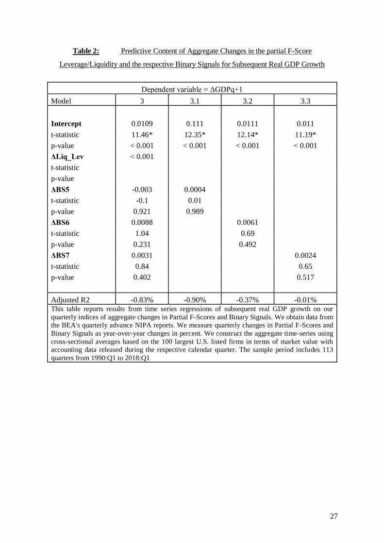
To further investigate the results, the liquidity/leverage variable is decomposed into its three
binary signals to determine precisely what exactly causes the variable to be a significant predictor.
Regarding Table 2 it is striking that neither grouped nor in isolation do the three binary signals

17
indicate predictive power for subsequent real GDP growth. The negative adjusted-R2 stresses
further the poor predictive ability of the explanatory variables. Thus, it appears likely that in
combination the liquidity/leverage variable is an accurate indicator for measuring individual firm
fundamentals, as advertised by Piotroski (2000). Hence, it becomes obvious that the set of
variables needs to be chosen carefully, as only when they are bundled as a grouped variable, the
predictive content becomes significant. Considering the operational efficiency Partial F-Score, the
insignificant results seem to be caused by two complementary effects. Firstly, while Konchitchki
and Patatoukas (2014) report that PM is a leading indicator for subsequent GDP growth, the results
of this study establish no significant predictive power, thus, it is obvious that a substantial amount
of information is lost during the transformation into the binary signals. Secondly, the chosen set
of variables for the profitability Partial F-Score is inappropriate to demonstrate predictive power
on the macro level. Konchitchki and Patatoukas (2014) indicate that ATO does not contain
predictive power to forecast subsequent macroeconomic growth. Consequently, the two binary
signals that comprise to the operational efficiency Partial F-Score do not complement each other.
One reason why ATO and thus operational efficiency are not a leading indicator for subsequent
GDP growth are their lagged effects on firm performance. Improvements in operational efficiency
do not cause an immediate effect but instead respond with a lag of several periods. As a
consequence, the variable does not contain predictive power for subsequent GDP growth. The
same reasoning holds for the profitability Partial F-Score, except that profitability related
improvements tend to show a sooner effect on firm performance. (Baik et al., 2013)
4.4 Incremental Predictive Power of Aggregate Changes in Total and Partial F-Scores
The collection and analysis of aggregate accounting data incurs non-trivial costs, while stock
market data are easily accessible and do not impose any costs on macroeconomic forecasters.
Hence, from a practical perspective, the analysis of aggregate accounting data can only be relevant
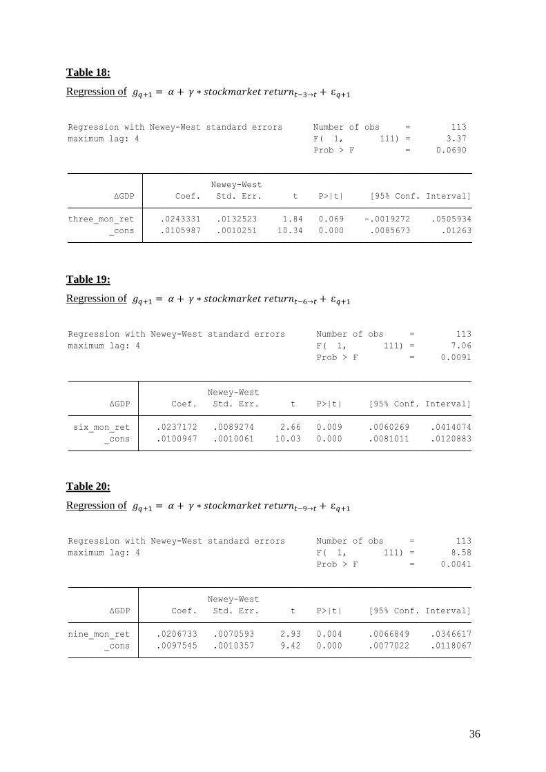
in terms of its incremental predictive power compared to stock market returns data. Table 6

18
suggests that one-year stock market returns provide the most powerful model to foresee
subsequent macroeconomic activity and are hence used as benchmark model. These findings are
in line with the research from Konchitchki and Patatoukas (2014).
Table 3 shows the respective results of Total F-Score (Model 4.1) as well as the liquidity and
leverage Partial F-Score (Model 4.2) as explanatory variables. Model 7.4 indicates, as expected,
that the one-year stock market return variable is a significant predictor for macroeconomic
activity. The adjusted-R2 is increased in comparison to Model 7.4 which only considers one-year
stock market returns as single explanatory variable. The goodness-of-fit measure increases from
20.77 % to 21.67 %. Hence, aggregate changes in Total F-Scores seem to indeed contain
incrementally useful information to predict subsequent macroeconomic activity. However, it
needs to be noted that the model only improves slightly and the contribution of the Total F-Score
is, at best, weakly significant so that any conclusions should be drawn carefully.
Similar observations can be made when considering Model 4.2, which includes the liquidity and
leverage Partial F-Score and one-year stock market returns as explanatory variables. The stock
market return variable is, again, significant, while the Partial F-Score is just like the Total F-Score
at best weakly significant as with a p-value of 0.15 it is not significant at the 90% confidence level.
The quality of the model, measured by the adjusted-R2, improves slightly from 20.77% to 21.37%.
Again, these findings need to be considered carefully as the added variable that is supposed to
cause the model improvement is, at best, weakly significant. Nevertheless, as the model fit
improves, it is assumed that aggregate changes in Total and Partial F-Score can have a positive
impact on macroeconomic forecasting, although this impact is minor.
4.5 The use of aggregate changes in Total and Partial F-Scores by macro forecasters
In Table 4 macroeconomic forecast revisions are chosen as dependent variable to investigate if
the professional forecasters adjust their projections according to newly available financial
statement data and consequently newly available changes in aggregate Total and Partial F-Scores.

19
The findings in Model 5.1 depict, as expected, significant results for the stock market returns
variable at the 99% confidence level, with a positive coefficient of 0.0221. The Total F-Score
coefficient indicates a positive coefficient of 0.0201 as well. However, the coefficient comes with,
at best, a weak statistical significance and a p-value of 0.153 and thus insignificant at the 90%
confidence level. Nevertheless, the quality of the model appears to have improved, as the adjusted-
R2 increases from 16.34% to 16.53% when stock market data are used in isolation to predict
forecast revisions from professional forecasters. Hence, it can be concluded that macroeconomic
forecasters are aware of some powerful information within aggregate Total F-Scores. However,
as the F-Score variable in Model 5.1 demonstrates, at best, a weak statistical significance,
conclusions should only be drawn with special considerations. The liquidity/leverage Partial F-
Score variable does not contain explanatory power forecast revisions. Thus, professional
forecasters do not seem to be aware of the incremental predictive power of this variable on
subsequent GDP growth. Consequently, the fourth hypothesis is rejected from the findings.
Another interesting observation that aligns with the findings of Konchitchki and Patatoukas
(2014) is that the intercepts of the discussed models are all significantly negative, revealing that
macroeconomic forecasters tend to revise their macroeconomic projections downwards as the
release date for the BEA NIPA report approaches. These findings are further evidence for the so-
called ‘walk-down’ phenomenon, associated with micro-level accounting research, which states
that an analyst’s optimism decreases as earnings reporting dates approach (Bamber, Barron, &
Stevens, 2011; Barron, Byard, Kim, 2002; Richardson, Teoh, & Wysocki, 2004).
4.6 Predictability of Forecast Errors on aggregate Changes in Total and Partial F-Scores
To examine whether forecasters are fully attuned to the examined variables and whether they can
help to minimise forecast errors, time series regressions on subsequent forecast errors with
aggregate changes in Total and Partial F-Scores and stock market returns data are conducted.

20
As weak statistical predictive power for forecast revisions in Total F-Scores is found, no
predictive power for subsequent forecast errors is expected. If macroeconomic forecasters are
aware of the predictive power of the variables and indeed utilise this information, the variables
would not sufficiently explain forecast errors, as the information would have already been
included in projections about subsequent macroeconomic activity. Consequently, the Total F-
Score variable is expected to contain no predictive power for subsequent forecast errors made by
professional forecasters. By assuming that the weak statistical significance of aggregate changes
in Total F-Scores for subsequent GDP growth and forecast revisions are valid, the results establish
that professionals consistently utilise information contained in aggregate changes of Total F-
Score. Moreover, as this study does not identify any predictive power of the liquidity/leverage
Partial F-Score variable on subsequent forecast revisions, significant predictive power of this
variable on forecast errors made by forecasters would suggest that professionals miss out on the
predictive power of aggregate changes in the liquidity/leverage Partial F-Score.
Regarding the examination of aggregate changes in Total F-Scores in isolation from stock market
returns data, no significant predictive power for subsequent forecast errors can be observed. With
a relatively high p-value of 0.198 and a very weak explanatory power for the total variation of the
dependent variable (adjusted-R2 0.87%), the results suggest either that forecasters are already fully
attuned to the leading information of aggregate changes in Total F-Scores or that aggregate
changes in Total F-Scores lack predictive power to explain GDP growth and thus forecast errors
or a combination of both. However, an, at best, statistically weak relationship between forecast
revisions and aggregate changes in Total F-Scores exists. By assuming that the weak statistical
predictive power of aggregate changes in Total F-Score on subsequent GDP growth is valid, the
results suggest that forecasters consistently utilise information included in this variable. Hence, it
is possible that professionals incorporate information about fundamental analysis in general,

21
which is correlated with aggregate changes in Total F-Scores despite potential information
outflow due to their binary nature.
Model 6.2 considers the liquidity/leverage Partial F-Score variable as single explanatory variable,
the coefficient of 0.0397 is positive and significant at the 99% confidence level. Moreover, the
adjusted-R2 increases greatly in comparison to Model 6.1 to 10.15%. Thus, aggregate changes in
the liquidity/leverage Partial F-Score explain 10.15% of the total variation of subsequent forecast
errors. These findings support the identified predictive power of the liquidity/leverage Partial F-
Score and reveal that forecasters do not integrate this information in their projections.
Moreover, stock market returns data are considered as single explanatory variable for subsequent
forecast errors. The findings do not align with Konchitchki and Patatoukas (2014), who find no
predictive power of stock market returns data on forecast errors. Several factors may explain these
contradictory findings. First, different time frames are considered; thus, circumstances and the
behaviour of macroeconomic forecasters, could have changed. Second, the contradictory findings
may result from forecasters making systematic errors. If this occurs, information that could
actually help to predict GDP growth may be excluded or improperly considered. Besides, stock
market returns data might include information that forecasters are unaware of, resulting in their
failure to fully consider them for projections about subsequent GDP growth. In addition,
forecasters may have adjusted their methods according to the findings of Konchitchki and
Patatoukas (2014) and have thus shifted their focus to aggregate accounting data and away from
relevant information from stock market returns. Nevertheless, this potential shift could only be
marginally responsible, as Konchitchki and Patatoukas’ (2014) findings were published in 2014
and could thus only affect the tests in a maximum of four of the nearly 30 years of observations.
Regarding the incremental usefulness of the liquidity/leverage variable after adding stock market
returns data as explanatory variable to the regression, the results suggest that the variable adds
incremental value. Both variables remain significant at the 99% confidence level, and the quality

22
of the model improves substantially, from an adjusted-R2 of 8.89% for stock market returns data
in isolation to 17.39% when considering both variables in the model.
The results fulfil the expectations. In Model 6.3, the liquidity/leverage variable shows a coefficient
of 0.0368 meaning that a one percent increase in the liquidity/leverage Partial F-Score is
associated with a 0.0368% increase in subsequent forecast errors. By assuming that the
incrementally useful and weak statistical predictive power of the variable on subsequent GDP
growth is valid, the results establish that forecasters fail to utilise the leading information of this
variable. The reason that forecast errors are predictable based on the liquidity/leverage Partial F-
Score and not the Total F-Score may also be rooted in the tendency of professionals to consider
fundamental analysis in general and thus be more attuned to Total F-Scores than to Partial F-
Scores. Compared to Konchitchki and Patatoukas (2014) who establish that macroeconomic
forecasters fully impound stock market returns data, this study finds different results, as stock
market returns data explains a significant part of subsequent forecast errors.
The findings establish either that forecasters are already fully attuned to aggregate changes in
Total F-Scores or that they do not contain predictive power for GDP growth, or a combination of
both. Moreover, a significant relationship between forecast errors and aggregate changes of the
liquidity/leverage Partial F-Score and stock market returns data is found. Both variables are
incrementally useful to predict forecast errors. The magnitudes of the estimated coefficients imply
that macroeconomic forecasts can be enhanced significantly. Hence, Hypothesis 5 is rejected.
5. Conclusion
This study is based upon a new stream of literature regarding the use of financial statement
analysis and macroeconomic forecasting. By utilising a sample of the top 100 US firms ranked by
MV, quarterly data on firm fundamentals, proxied by Total and Partial F-Scores, is aggregated.
The results suggest, at best, that aggregate changes in Total F-Scores have weak predictive power,
which fails to be significant at the 85% confidence level. By investigating the three Partial F-

23
Scores, only the liquidity/leverage Partial F-Score variable proves to contain significant predictive
power for subsequent macroeconomic growth. The inclusion of the stock market variable puts
pressure on the significance of the liquidity/leverage Partial F-Score, suggesting that a substantial
portion of the information is already captured by stock market returns data.
Testing for the predictive power of Partial F-Scores on forecast revisions establishes that
professionals do not integrate information on the liquidity/leverage variable into their projections,
and, at best, some information that is contained within aggregate changes of Total F-Scores.
As final step the predictive power on subsequent forecast errors is assessed. As this study
does not find predictive power of the liquidity/leverage Partial F-Score variable on subsequent
forecast revisions, but on subsequent real GDP growth and forecast errors, the results suggest that
forecasters miss out on the predictive power of aggregate changes in liquidity/ leverage Partial F-
Scores and the potential to improve their projections.
5.1 Limitations
Certainly, the conducted study comes with limitations and needs to be considered with
reservations. Firstly, the data set needed to be thinned out due to missing data for individual
companies and variables. Roughly about one-fourth of the considered companies had to be
eliminated and replaced by the next largest company based on MV in the respective quarter. Some
of these unanalysed companies were very influential to the economy.
Secondly, as binary variables were analysed, it is conceivable that the analysed variables over- or
underestimate the actual effects. The insignificance of the binary signal representing aggregate
changes in PM on subsequent macroeconomic growth, serves as a clear indication that substantial
information is lost during the transformation.
Thirdly, Financial statements are, according to GAAP, nominal. Konchitchki (2013) finds
inflation-based investment strategies yielding abnormal returns, resulting from investors who

24
incorrectly estimate the effects of inflation. If this theory proves to be correct and the market does
miss the effect of inflation, it has a significant influence on the financials and value of companies.
Finally, the methodology applied in this study differs slightly from the original.
Konchitchki and Patatoukas (2014) align fiscal quarters with calendar quarters to create a timely
match between the time of publishing accounting data and distributing SPF questionnaires. In this
study, calendar quarters are assumed, thus financial statements available until the end of the
calendar quarter are considered. This approach reduces the number of firms that must be excluded
and captures a more representative sample of the top 100 companies in the US. However, it creates
a slight mismatch between released accounting data and the distribution of the SPF questionnaires.
Hence, the aggregate accounting data used as explanatory variables were, at best, published one
month before the distribution of the questionnaires. This might affect the predictive power of the
explanatory variables, as the most recent events are not included in the explanatory variables.
5.2 Future Research
Macroeconomic forecasting will never be complete but will continuously be developed and
refined. Before Konchitchki and Patatoukas (2014) published their findings, professionals were
not aware that aggregate accounting data contain predictive power for macroeconomic growth.
The transformation into binary signals should be further studied to assess the impact of the
information loss. Moreover, alternative financial metrics should be analysed to assess their
usefulness for macroeconomic forecasting and optimise resource allocations in the economy.
As the sample size of 100 firms appears to be sufficiently large to contain predictive power
for the entire economy, it is of great interest whether the sample size could further be reduced.
The ambiguous results about the predictive power of stock market returns data on forecast
errors, compared to the findings of Konchitchki and Patatoukas (2014), should be further
investigated to detect potential biases or shifts in forecasting methodology.

25
6. References
Baik, B., Chae, J., Choi, S. & Farber, D. B. (2013). Changes in Operational Efficiency and Firm Performance: A Frontier Analysis
Approach. Contemporary Accounting Research, 30(3). 996-1026. doi:10.1111/j.1911-3846.2012.01179.x
Bamber, L. S., Barron, O. E. & Stevens, D. E. (2011). Trading Volume Around Earnings Announcements and Other Financial
Reports: Theory, Research Design, Empirical Evidence, and Directions for Future Research. Contemporary Accounting
Research, 28(2). 431-471. doi:10.1111/j.1911-3846.2010.01061.x
Barron, O. E., Byard D., & Kim O. (2002). Changes in Analysts' Information around Earnings Announcements. The Accounting
Review, 77(4), 821-846.
Baumann, M. P. (2014). Forecasting operating Profitability with DuPont Analysis: Further Evidence. Review of Accounting and
Finance, 13(2), 191-205.
Berk J. & DeMarzo P. (2014). Corporate Finance (3rd ed.). Harlow: Pearson Education Limited.
Bratu, M. (2012). Point Forecasts based on the Limits of the Forecast Intervals to improve the SPF Predictions. Business and
Economic Horizons, 8(2), 1-11.
Carlin W. & Soskice D. (2015). Macroeconomics – Institutions, Instability and the Financial System (3rd ed.). New York, NY:
Oxford University Press.
Croushore, D. (2010). An Evaluation of Inflation Forecasts from Surveys Using Real-Time Data. The B.E. Journal
Macroeconomics, 10(1), 1935-1960 DOI: 10.2202/1935-1690.1677
Dechow, P. (1994). Accounting Earnings and Cash Flows as Measures of Firm Performance: The Role of Accounting Accruals.
Journal of Accounting and Economics, 18(1), 3-42.
Fairfield, P. M. & Yohn T. L. (2001). Using Asset Turnover and Profit Margin to forecast Changes in Profitability. Review of
Accounting Studies, 6(4), 371-385.
Fama, E. F. (1990). Stock Returns, expected Returns, and real Activity. The Journal of Finance, 45(4), 1089-1108.
Fama, E. F., & French, K. R. (1992). The Cross-section of expected Returns. The Journal of Finance, 47(2), 427-465.
Federal Reserve Bank of Philadelphia. (2018, August 29) Survey of Professional Forecasters. Retrieved from
https://www.philadelphiafed.org/research-and-data/real-time-center/survey-of-professional-forecasters/
Fildes, R., Stekler, H. (2002). The state of macroeconomic forecasting. Journal of Macroeconomics, 24(4), 435-468.
Ivanov K., (2016). Taking the pulse of the real economy III: Sharpening macro forecasts with the debt point of view.
MaastrichtUniversity School of Business and Economics.
Kalay, A., Nallareddy, S. & Sadka.G. (2018). Uncertainty and sectoral shifts: The Interaction between Firm-Level and Aggregate-
Level Shocks, and Macroeconomic Activity. Management Science 64 (1): 198–214.
Kieso, D., Weygandt, J. and Warfield, T. (2014). Intermediate Accounting (2nd ed.). Hoboken: John Wiley & Sons, Inc.
Konchitchki, Y. (2013). Accounting and the Macroeconomy: The Case of Aggregate Price-Level Effects on Individual Stocks.
Financial Analysis Journal, 69(6), 40-54.
Konchitchki, Y., & Patatoukas, P. N. (2014). Taking the pulse of the real economy using financial statement analysis: Implications
for macro forecasting and stock valuation. The Accounting Review, 89(2), 669-694.
Konchitchki, Y., & Patatoukas, P. N. (2014). Accounting Earnings and Gross Domestic Product. Journal of Accounting and
Economics, 57(1), 76-88.
Moehrle, S. R., Anderson, K. L. Ayres, F. L., Bolt-Lee, C. E., Debreceny, R. S., Dugan, M. T. & Plummer, E. (2009). The Impact
of Academic Accounting Research on Professional Practice: An Analysis by the AAA Research Impact Task Force.
Accounting Horizons, 23(4), 411-456.
Newey, W. K., & West, K. D. (1987). A Simple Positive, Semi-definite, Heteroscedasticity and Autocorrelation consistent
Covariance Matrix. Economtrica, 55(3), 703-708.
Ou, J. A., & Penman, S. H. (1989). Financial statement analysis and the Prediction of Stock Returns. Journal of Accounting and
Economics 11(4), 295-329.
Palepu, K., Healy, P. and Peek, E. (2016). Business analysis and valuation (4th ed.). Andover: Cengage Learning EMEA.
Piotroski, J. D. (2000). Value Investing: The Use of Historical Financial Statement Information to Separate Winners from Losers.
Journal of Accounting Research Center, 38(1), 1-41.
Piotroski, J. D. & So, E. C. (2012). Identifying Expectation Errors in Value/Glamour Strategies: A Fundamental Analysis Approach.
The Review of Financial Studies, 25(9), 2841-2875.
Richardson, S., Teoh, S. H. & Wysocki, P.D. (2004). The walk-down to beatable analyst Forecasts: The Role of Equity Issuance
and Insider Trading incentives. Contemporary Accounting Research, 21(4). 885-924-
Sharpe, N., DeVeaux, R. D., Vellemann, P. (2012). Business Statistics (2nd ed.). Boston, MA: Pearson Education Inc.
Soliman, M. T. (2008). The Use of DuPont Analysis by Market Participants. The Accounting Review, 83(3), 823-853.
Sloan, R. G, (1996). “Do Stock Prices fully reflect Information in Accruals and Cash Flows about Future Earnings?” The Accounting
Review, 71(3), 289-315.
Wieland, V., Wolters, M. (2011). The Diversity of Forecasts from Macroeconomic Models of the US Economy. Economic Theory
47(2/3), 247-292.

26
8. Appendix
Table 1: Predictive Content of Aggregate Changes in Total F-Score and Partial F-Scores
for Subsequent Real GDP Growth
Dependent variable = ΔGDPq+1
Model 1 2 2.1 2.2 2.3
Intercept 0.011 0.011 0.111 0.0108 0.111
t-statistic 12.02* 11.78* 11.54* 12.44* 11.82*
p-value < 0.001 < 0.001 < 0.001 < 0.001 < 0.001
ΔTotal_FScore 0.02
t-statistic 1.39
p-value 0.167
ΔProfitability 0.0036 0.57
t-statistic 0.28 0.569
p-value 0.783 0.0078
ΔLiq_Lev 0.0104 0.0109
t-statistic 2.41* 2.35*
p-value 0.018 0.02
ΔOperational_Eff 0.0023 0.003
t-statistic 0.39 0.49
p-value 0.695 0.624
Adjusted R2 0.93% -0.18% -0.60% 1.45% -0.73%
This table reports results from time series regressions of subsequent real GDP growth on our quarterly
indices of aggregate changes in Total F-Score and Partial F-Scores. We obtain data from the BEA's quarterly
advance NIPA reports. We measure quarterly changes in Total F-Score and Partial F-Scores as year-over-
year changes in percent. We construct the aggregate time-series using cross-sectional averages based on the
100 largest U.S. listed firms in terms of market value with accounting data released during the respective
calendar quarter. The sample period includes 113 quarters from 1990:Q1 to 2018:Q1
27
Table 2: Predictive Content of Aggregate Changes in the partial F-Score
Leverage/Liquidity and the respective Binary Signals for Subsequent Real GDP Growth
Dependent variable = ΔGDPq+1
Model 3 3.1 3.2 3.3
Intercept 0.0109 0.111 0.0111 0.011
t-statistic 11.46* 12.35* 12.14* 11.19*
p-value < 0.001 < 0.001 < 0.001 < 0.001
ΔLiq_Lev < 0.001
t-statistic
p-value
ΔBS5 -0.003 0.0004
t-statistic -0.1 0.01
p-value 0.921 0.989
ΔBS6 0.0088 0.0061
t-statistic 1.04 0.69
p-value 0.231 0.492
ΔBS7 0.0031 0.0024
t-statistic 0.84 0.65
p-value 0.402 0.517
Adjusted R2 -0.83% -0.90% -0.37% -0.01% This table reports results from time series regressions of subsequent real GDP growth on our
quarterly indices of aggregate changes in Partial F-Scores and Binary Signals. We obtain data from
the BEA's quarterly advance NIPA reports. We measure quarterly changes in Partial F-Scores and
Binary Signals as year-over-year changes in percent. We construct the aggregate time-series using
cross-sectional averages based on the 100 largest U.S. listed firms in terms of market value with
accounting data released during the respective calendar quarter. The sample period includes 113
quarters from 1990:Q1 to 2018:Q1

28
Table 3: Incremental Predictive Content of Aggregate Changes in Total F-Score and
Partial F-Scores and Stock Market Returns for Subsequent Real GDP Growth
Dependent variable = ΔGDPq+1
Model 4.1 4.2 7.4
Intercept 0.0094 0.0094 0.0095
t-statistic 9.18* 8.94* 8.61*
p-value < 0.001 < 0.001 < 0.001
ΔTotal_FScore 0.019
t-statistic 1.55
p-value 0.125
ΔLiq_Lev 0.0081
t-statistic 1.45
p-value 0.15
one_year_ret 0.0179 0.017 0.0181
t-statistic 3.12* 2.91* 2.96*
p-value 0.002 0.004 0.004
Adjusted R2 21.67% 21.37% 20.77%
This table reports results from time series regressions of subsequent real GDP growth on our quarterly
indices of aggregate changes in Partial F-Scores and Binary Signals. We obtain data from the BEA's
quarterly advance NIPA reports. We measure quarterly changes in Partial F-Scores and Binary
Signals as year-over-year changes in percent. We construct the aggregate time-series using cross-
sectional averages based on the 100 largest U.S. listed firms in terms of market value with accounting
data released during the respective calendar quarter. The Stock market returns are measured over one
year. The stock market portfolio is proxied by the S&P 500 index sample period includes 113 quarters
from 1990:Q1 to 2018:Q1

29
Table 4: Association of Revisions in Expectations about Subsequent Real GDP Growth
with Aggregate Changes in Total F-Score and Partial F-Scores and Stock Market Returns
Dependent variable = Forecast Revisions (FR)
Model 5.1 5.2 5.3
Intercept -0.0024 -0.0023 -0.0023
t-statistic -2.86* -2.81* -2.72*
p-value 0.005 0.06 0.007
ΔTotal_FScore 0.0201
t-statistic 1.44
p-value 0.153
ΔLiq_Lev 0.0068
t-statistic 0.87
p-value 0.388
one_year_ret 0.0221 0.0281 0.0222
t-statistic 5.48* 5.35* 5.20*
p-value < 0.001 < 0.001 < 0.001
Adjusted R2 16.53% 16.07% 16.34%
This table reports results from time series regressions of subsequent real GDP growth on our
quarterly indices of aggregate changes in Partial F-Scores and Binary Signals. We obtain data
from the BEA's quarterly advance NIPA reports. We measure quarterly changes in Partial F-
Scores and Binary Signals as year-over-year changes in percent. We construct the aggregate time-
series using cross-sectional averages based on the 100 largest U.S. listed firms in terms of market
value with accounting data released during the respective calendar quarter. The Stock market
returns are measured over one year. The stock market portfolio is proxied by the S&P 500 index
sample period includes 113 quarters from 1990:Q1 to 2018:Q1

30
Table 5: Predictive Content of Aggregate Changes in Total F-Scores and Partial F-Scores
and Stock Market Returns for Subsequent Real GDP Growth Forecast Errors
Dependent variable = Forecast Errors (FE)
Model 6.1 6.2 6.3 6.4
Intercept 0.0007 0.0006 -0.001 -0.001
t-statistic 0.46 0.42 -0.74 -0.66
p-value 0.644 0.677 0.461 0.513
ΔTotal_FScore 0.0336
t-statistic 1.29
p-value 0.198
ΔLiq_Lev 0.0397 0.0368
t-statistic 3.95* 4.40*
p-value < 0.001 < 0.001
one_year_ret 0.0185 0.0202
t-statistic 3.38* 3.89*
p-value 0.001 < 0.001
Adjusted R2 0.87% 10.15% 17.39% 8.69%
This table reports results from time series regressions of subsequent real GDP growth forecast errors on
our quarterly indices of aggregate changes in Partial F-Scores and Binary Signals and stock market
returns. We measure subsequent real GDP growth forecast errors as the difference between subsequent
real GDP growth and the corresponding mean consensus forecast as of quarter q from the SPF. We obtain
data from the BEA's quarterly advance NIPA reports. We obtain the SPF mean consensus forecasts of
real GDP growth from the Federal Reserve Bank of Philadelphia. We measure quarterly changes in
Partial F-Scores and Binary Signals as year-over-year changes in percent. We construct the aggregate
time-series using cross-sectional averages based on the 100 largest U.S. listed firms in terms of market
value with accounting data released during the respective calendar quarter. The Stock market returns are
measured over one year. The stock market portfolio is proxied by the S&P 500 index sample period
includes 113 quarters from 1990:Q1 to 2018:Q1

31
Table 6: Predictive Content of Stock Market Returns (Proxy: S&P 500) for Subsequent
Real GDP Growth
Dependent variable = ΔGDPq+1
Model 7.1 7.2 7.3 7.4 7.5
Intercept 0.106 0.0101 0.0098 0.0095 0.0095
t-statistic 10.34* 10.03* 9.42* 8.61* 7.06*
p-value < 0.001 < 0.001 < 0.001 < 0.001 < 0.001
three_mon_ret 0.2433
t-statistic 1.84
p-value 0.069
six_mon_ret 0.0237
t-statistic 2.66*
p-value 0.009
nine_mon_ret 0.2067
t-statistic 2.93*
p-value 0.004
one_year_ret 0.0181
t-statistic 2.96*
p-value 0.004
two_year_ret 0.0082
t-statistic 2.33*
p-value 0.022
Adjusted R2 7.46% 15.95% 19.35% 20.77% 10.53%
This table reports results from time series regressions of subsequent real GDP growth on buy-and-
hold stock market returns. Stock market returns are measured over 3-, 6-, 9-, 12- & 24-month periods.
We obtain data on real GDP growth from BEA's quarterly advance NIPA reports. The S&P 500 index
is used as proxy for the stock market portfolio The sample period includes 113 quarters from 1990:Q1
to 2018:Q1

32
Table 7: Descriptive Statistics
Table 8: Pairwise Correlations

33
Table 9:
Regression of 𝑔𝑞+1 = 𝛼 + 𝛽1 × ΔA𝑔𝑔𝑟𝑒𝑔𝑎𝑡𝑒 𝑇𝑜𝑡𝑎𝑙 𝐹𝑆𝑐𝑜𝑟𝑒𝑞 + 𝑞+1
Table 10:
Regression of 𝑔𝑞+1 = 𝛼 + Σ 𝛽𝑘 × Δ𝐴𝑔𝑔𝑟𝑒𝑔𝑎𝑡𝑒 𝑃𝑎𝑟𝑡𝑖𝑎𝑙 𝐹𝑆𝑐𝑜𝑟𝑒𝑠𝑞𝑘 + 𝑞+1
Table 11:
Regression of 𝑔𝑞+1 = 𝛼 + × 𝛽1 ΔA𝑔𝑔𝑟𝑒𝑔𝑎𝑡𝑒 𝑃𝑟𝑜𝑓𝑖𝑡𝑎𝑏𝑖𝑙𝑖𝑡𝑦 𝑃𝑎𝑟𝑡𝑖𝑎𝑙 𝐹𝑆𝑐𝑜𝑟𝑒𝑞 + 𝑞+1
_cons .0110311 .000918 12.02 0.000 .0092121 .0128502
ΔTotal_FScore .0203045 .0146001 1.39 0.167 -.0086265 .0492355
ΔGDP Coef. Std. Err. t P>|t| [95% Conf. Interval]
Newey-West
Prob > F = 0.1671
maximum lag: 4 F( 1, 111) = 1.93
Regression with Newey-West standard errors Number of obs = 113
_cons .0110136 .0009353 11.78 0.000 .0091599 .0128673
ΔOperationa~f .0022495 .0057254 0.39 0.695 -.009098 .013597
ΔLiq_Lev .0104209 .0043308 2.41 0.018 .0018374 .0190044
ΔProfitabil~y .00362 .013094 0.28 0.783 -.0223319 .0295718
ΔGDP Coef. Std. Err. t P>|t| [95% Conf. Interval]
Newey-West
Prob > F = 0.1260
maximum lag: 4 F( 3, 109) = 1.95
Regression with Newey-West standard errors Number of obs = 113
_cons .0110692 .000959 11.54 0.000 .0091689 .0129694
ΔProfitabil~y .0077981 .0136676 0.57 0.569 -.0192851 .0348813
ΔGDP Coef. Std. Err. t P>|t| [95% Conf. Interval]
Newey-West
Prob > F = 0.5695
maximum lag: 4 F( 1, 111) = 0.33
Regression with Newey-West standard errors Number of obs = 113
34
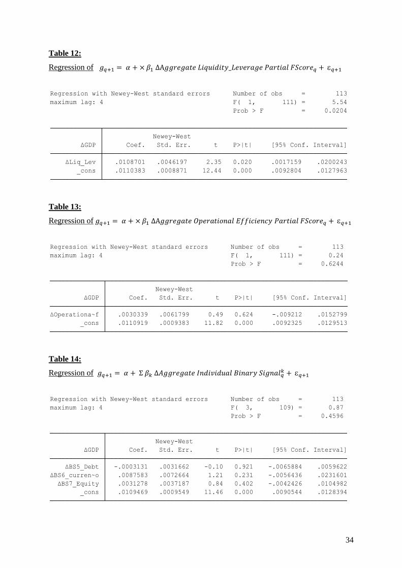
Table 12:
Regression of 𝑔𝑞+1 = 𝛼 + × 𝛽1 ΔA𝑔𝑔𝑟𝑒𝑔𝑎𝑡𝑒 𝐿𝑖𝑞𝑢𝑖𝑑𝑖𝑡𝑦_𝐿𝑒𝑣𝑒𝑟𝑎𝑔𝑒 𝑃𝑎𝑟𝑡𝑖𝑎𝑙 𝐹𝑆𝑐𝑜𝑟𝑒𝑞 + 𝑞+1
Table 13:
Regression of 𝑔𝑞+1 = 𝛼 + × 𝛽1 ΔA𝑔𝑔𝑟𝑒𝑔𝑎𝑡𝑒 𝑂𝑝𝑒𝑟𝑎𝑡𝑖𝑜𝑛𝑎𝑙 𝐸𝑓𝑓𝑖𝑐𝑖𝑒𝑛𝑐𝑦 𝑃𝑎𝑟𝑡𝑖𝑎𝑙 𝐹𝑆𝑐𝑜𝑟𝑒𝑞 + 𝑞+1
Table 14:
Regression of 𝑔𝑞+1 = 𝛼 + Σ 𝛽𝑘 Δ𝐴𝑔𝑔𝑟𝑒𝑔𝑎𝑡𝑒 𝐼𝑛𝑑𝑖𝑣𝑖𝑑𝑢𝑎𝑙 𝐵𝑖𝑛𝑎𝑟𝑦 𝑆𝑖𝑔𝑛𝑎𝑙𝑞𝑘 + 𝑞+1
_cons .0110383 .0008871 12.44 0.000 .0092804 .0127963
ΔLiq_Lev .0108701 .0046197 2.35 0.020 .0017159 .0200243
ΔGDP Coef. Std. Err. t P>|t| [95% Conf. Interval]
Newey-West
Prob > F = 0.0204
maximum lag: 4 F( 1, 111) = 5.54
Regression with Newey-West standard errors Number of obs = 113
_cons .0110919 .0009383 11.82 0.000 .0092325 .0129513
ΔOperationa~f .0030339 .0061799 0.49 0.624 -.009212 .0152799
ΔGDP Coef. Std. Err. t P>|t| [95% Conf. Interval]
Newey-West
Prob > F = 0.6244
maximum lag: 4 F( 1, 111) = 0.24
Regression with Newey-West standard errors Number of obs = 113
_cons .0109469 .0009549 11.46 0.000 .0090544 .0128394
ΔBS7_Equity .0031278 .0037187 0.84 0.402 -.0042426 .0104982
ΔBS6_curren~o .0087583 .0072664 1.21 0.231 -.0056436 .0231601
ΔBS5_Debt -.0003131 .0031662 -0.10 0.921 -.0065884 .0059622
ΔGDP Coef. Std. Err. t P>|t| [95% Conf. Interval]
Newey-West
Prob > F = 0.4596
maximum lag: 4 F( 3, 109) = 0.87
Regression with Newey-West standard errors Number of obs = 113

35
Table 15:
Regression of 𝑔𝑞+1 = 𝛼 + × 𝛽1 ΔAggregate BS5_Debt𝑞 + 𝑞+1
Table 16:
Regression of 𝑔𝑞+1 = 𝛼 + × 𝛽1 ΔAggregate BS6_Currentratio𝑞 + 𝑞+1
Table 17:
Regression of 𝑔𝑞+1 = 𝛼 + × 𝛽1 ΔAggregate BS7_Equity𝑞 + 𝑞+1
_cons .0111053 .0008991 12.35 0.000 .0093237 .012887
ΔBS5_Debt .0000441 .0032979 0.01 0.989 -.0064909 .0065792
ΔGDP Coef. Std. Err. t P>|t| [95% Conf. Interval]
Newey-West
Prob > F = 0.9893
maximum lag: 4 F( 1, 111) = 0.00
Regression with Newey-West standard errors Number of obs = 113
_cons .0110844 .0009132 12.14 0.000 .0092747 .012894
ΔBS6_curren~o .0061311 .0088912 0.69 0.492 -.0114875 .0237496
ΔGDP Coef. Std. Err. t P>|t| [95% Conf. Interval]
Newey-West
Prob > F = 0.4919
maximum lag: 4 F( 1, 111) = 0.48
Regression with Newey-West standard errors Number of obs = 113
_cons .0110013 .0009835 11.19 0.000 .0090524 .0129501
ΔBS7_Equity .0024606 .003788 0.65 0.517 -.0050455 .0099668
ΔGDP Coef. Std. Err. t P>|t| [95% Conf. Interval]
Newey-West
Prob > F = 0.5173
maximum lag: 4 F( 1, 111) = 0.42
Regression with Newey-West standard errors Number of obs = 113
36
Table 18:
Regression of 𝑔𝑞+1 = 𝛼 + 𝛾 ∗ 𝑠𝑡𝑜𝑐𝑘𝑚𝑎𝑟𝑘𝑒𝑡 𝑟𝑒𝑡𝑢𝑟𝑛𝑡−3→𝑡 + 𝑞+1
Table 19:
Regression of 𝑔𝑞+1 = 𝛼 + 𝛾 ∗ 𝑠𝑡𝑜𝑐𝑘𝑚𝑎𝑟𝑘𝑒𝑡 𝑟𝑒𝑡𝑢𝑟𝑛𝑡−6→𝑡 + 𝑞+1
Table 20:
Regression of 𝑔𝑞+1 = 𝛼 + 𝛾 ∗ 𝑠𝑡𝑜𝑐𝑘𝑚𝑎𝑟𝑘𝑒𝑡 𝑟𝑒𝑡𝑢𝑟𝑛𝑡−9→𝑡 + 𝑞+1
_cons .0105987 .0010251 10.34 0.000 .0085673 .01263
three_mon_ret .0243331 .0132523 1.84 0.069 -.0019272 .0505934
ΔGDP Coef. Std. Err. t P>|t| [95% Conf. Interval]
Newey-West
Prob > F = 0.0690
maximum lag: 4 F( 1, 111) = 3.37
Regression with Newey-West standard errors Number of obs = 113
_cons .0100947 .0010061 10.03 0.000 .0081011 .0120883
six_mon_ret .0237172 .0089274 2.66 0.009 .0060269 .0414074
ΔGDP Coef. Std. Err. t P>|t| [95% Conf. Interval]
Newey-West
Prob > F = 0.0091
maximum lag: 4 F( 1, 111) = 7.06
Regression with Newey-West standard errors Number of obs = 113
_cons .0097545 .0010357 9.42 0.000 .0077022 .0118067
nine_mon_ret .0206733 .0070593 2.93 0.004 .0066849 .0346617
ΔGDP Coef. Std. Err. t P>|t| [95% Conf. Interval]
Newey-West
Prob > F = 0.0041
maximum lag: 4 F( 1, 111) = 8.58
Regression with Newey-West standard errors Number of obs = 113
37
Table 21:
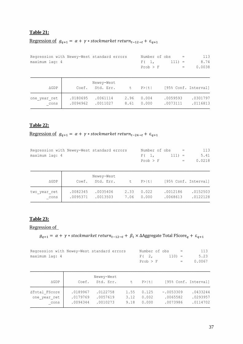
Regression of 𝑔𝑞+1 = 𝛼 + 𝛾 ∗ 𝑠𝑡𝑜𝑐𝑘𝑚𝑎𝑟𝑘𝑒𝑡 𝑟𝑒𝑡𝑢𝑟𝑛𝑡−12→𝑡 + 𝑞+1
Table 22:
Regression of 𝑔𝑞+1 = 𝛼 + 𝛾 ∗ 𝑠𝑡𝑜𝑐𝑘𝑚𝑎𝑟𝑘𝑒𝑡 𝑟𝑒𝑡𝑢𝑟𝑛𝑡−24→𝑡 + 𝑞+1
Table 23:
Regression of
𝑔𝑞+1 = 𝛼 + 𝛾 ∗ 𝑠𝑡𝑜𝑐𝑘𝑚𝑎𝑟𝑘𝑒𝑡 𝑟𝑒𝑡𝑢𝑟𝑛𝑡−12→𝑡 + 𝛽1 × ΔAggregate Total FScore𝑞 + 𝑞+1
_cons .0094962 .0011027 8.61 0.000 .0073111 .0116813
one_year_ret .0180695 .0061114 2.96 0.004 .0059593 .0301797
ΔGDP Coef. Std. Err. t P>|t| [95% Conf. Interval]
Newey-West
Prob > F = 0.0038
maximum lag: 4 F( 1, 111) = 8.74
Regression with Newey-West standard errors Number of obs = 113
_cons .0095371 .0013503 7.06 0.000 .0068613 .0122128
two_year_ret .0082345 .0035406 2.33 0.022 .0012186 .0152503
ΔGDP Coef. Std. Err. t P>|t| [95% Conf. Interval]
Newey-West
Prob > F = 0.0218
maximum lag: 4 F( 1, 111) = 5.41
Regression with Newey-West standard errors Number of obs = 113
_cons .0094344 .0010273 9.18 0.000 .0073986 .0114702
one_year_ret .0179769 .0057619 3.12 0.002 .0065582 .0293957
ΔTotal_FScore .0189967 .0122758 1.55 0.125 -.0053309 .0433244
ΔGDP Coef. Std. Err. t P>|t| [95% Conf. Interval]
Newey-West
Prob > F = 0.0067
maximum lag: 4 F( 2, 110) = 5.23
Regression with Newey-West standard errors Number of obs = 113

38
Table 24:
Regression of
𝑔𝑞+1 = 𝛼 + 𝛾 ∗ 𝑠𝑡𝑜𝑐𝑘𝑚𝑎𝑟𝑘𝑒𝑡 𝑟𝑒𝑡𝑢𝑟𝑛𝑡−12→𝑡
+ 𝛽1 × ΔAggregate Liquidity_Leverage Partial FScore𝑞 + 𝑞+1
Table 25:
Regression of 𝐸𝑞[𝑔𝑞+1] − 𝐸𝑞−1[𝑔𝑞+1] =
𝛼 + 𝛾 ∗ 𝑠𝑡𝑜𝑐𝑘𝑚𝑎𝑟𝑘𝑒𝑡 𝑟𝑒𝑡𝑢𝑟𝑛𝑡−𝑘→𝑡 + 𝛽1 × ΔAggregate Total FScore𝑞 + 𝑞+1
_cons .0094792 .0010608 8.94 0.000 .0073769 .0115815
one_year_ret .017692 .0060845 2.91 0.004 .0056341 .02975
ΔLiq_Lev .0081351 .0056067 1.45 0.150 -.002976 .0192462
ΔGDP Coef. Std. Err. t P>|t| [95% Conf. Interval]
Newey-West
Prob > F = 0.0017
maximum lag: 4 F( 2, 110) = 6.76
Regression with Newey-West standard errors Number of obs = 113
_cons -.0023515 .0008231 -2.86 0.005 -.0039827 -.0007203
one_year_ret .0220613 .0040271 5.48 0.000 .0140805 .0300422
ΔTotal_FScore .020087 .013963 1.44 0.153 -.0075844 .0477584
F_Revision Coef. Std. Err. t P>|t| [95% Conf. Interval]
Newey-West
Prob > F = 0.0000
maximum lag: 4 F( 2, 110) = 16.48
Regression with Newey-West standard errors Number of obs = 113

39
Table 26:
Regression of 𝐸𝑞[𝑔𝑞+1] − 𝐸𝑞−1[𝑔𝑞+1] =
𝛼 + 𝛾 ∗ 𝑠𝑡𝑜𝑐𝑘𝑚𝑎𝑟𝑘𝑒𝑡 𝑟𝑒𝑡𝑢𝑟𝑛𝑡−𝑘→𝑡 + 𝛽1 × ΔAggregate Liquidity_Leverage Partial FScore
+ 𝑞+1
Table 27:
Regression of
𝐸𝑞[𝑔𝑞+1] − 𝐸𝑞−1[𝑔𝑞+1] = 𝛼 + 𝛾 ∗ 𝑠𝑡𝑜𝑐𝑘𝑚𝑎𝑟𝑘𝑒𝑡 𝑟𝑒𝑡𝑢𝑟𝑛𝑡−𝑘→𝑡 + 𝑞+1
_cons -.0023004 .0008191 -2.81 0.006 -.0039236 -.0006772
one_year_ret .0218429 .0040849 5.35 0.000 .0137477 .0299382
ΔLiq_Lev .0068167 .0078618 0.87 0.388 -.0087636 .0223969
F_Revision Coef. Std. Err. t P>|t| [95% Conf. Interval]
Newey-West
Prob > F = 0.0000
maximum lag: 4 F( 2, 110) = 14.30
Regression with Newey-West standard errors Number of obs = 113
_cons -.0022862 .0008391 -2.72 0.007 -.003949 -.0006233
one_year_ret .0221592 .0042582 5.20 0.000 .0137212 .0305972
F_Revision Coef. Std. Err. t P>|t| [95% Conf. Interval]
Newey-West
Prob > F = 0.0000
maximum lag: 4 F( 1, 111) = 27.08
Regression with Newey-West standard errors Number of obs = 113

40
Table 28:
Regression of
𝑔𝑞+1 − 𝐸𝑞[𝑔𝑞+1] = 𝛼 + 𝛽1 × ΔAggregate Total FScore𝑞 + 𝑞+1
Table 29:
Regression of
𝑔𝑞+1 − 𝐸𝑞[𝑔𝑞+1] = 𝛼 + 𝛽1 × ΔAggregate Liquidity_Leverage Partial FScore + 𝑞+1
_cons .0007108 .0015318 0.46 0.644 -.0023245 .0037462
ΔTotal_FScore .0336295 .0259912 1.29 0.198 -.0178739 .0851329
F_Error Coef. Std. Err. t P>|t| [95% Conf. Interval]
Newey-West
Prob > F = 0.1984
maximum lag: 4 F( 1, 111) = 1.67
Regression with Newey-West standard errors Number of obs = 113
_cons .0005877 .0014078 0.42 0.677 -.0022019 .0033774
ΔLiq_Lev .0396919 .0100497 3.95 0.000 .0197778 .059606
F_Error Coef. Std. Err. t P>|t| [95% Conf. Interval]
Newey-West
Prob > F = 0.0001
maximum lag: 4 F( 1, 111) = 15.60
Regression with Newey-West standard errors Number of obs = 113

41
Table 30:
Regression of 𝑔𝑞+1 − 𝐸𝑞[𝑔𝑞+1] =
𝛼 + 𝛾 ∗ 𝑠𝑡𝑜𝑐𝑘𝑚𝑎𝑟𝑘𝑒𝑡 𝑟𝑒𝑡𝑢𝑟𝑛𝑡−𝑘→𝑡 + 𝛽1 × ΔAggregate Liquidity_Leverage Partial FScore
+ 𝑞+1
Table 31:
Regression of 𝑔𝑞+1 − 𝐸𝑞[𝑔𝑞+1] =
𝛼 + 𝛾 ∗ 𝑠𝑡𝑜𝑐𝑘𝑚𝑎𝑟𝑘𝑒𝑡 𝑟𝑒𝑡𝑢𝑟𝑛𝑡−𝑘→𝑡 + 𝑞+1
_cons -.001047 .0014148 -0.74 0.461 -.0038509 .0017569
one_year_ret .01855 .0054834 3.38 0.001 .0076832 .0294168
ΔLiq_Lev .0368243 .0083762 4.40 0.000 .0202246 .0534239
F_Error Coef. Std. Err. t P>|t| [95% Conf. Interval]
Newey-West
Prob > F = 0.0000
maximum lag: 4 F( 2, 110) = 25.44
Regression with Newey-West standard errors Number of obs = 113
_cons -.00097 .0014793 -0.66 0.513 -.0039013 .0019613
one_year_ret .0202587 .0052073 3.89 0.000 .0099401 .0305772
F_Error Coef. Std. Err. t P>|t| [95% Conf. Interval]
Newey-West
Prob > F = 0.0002
maximum lag: 4 F( 1, 111) = 15.14
Regression with Newey-West standard errors Number of obs = 113

42
Table 32: Dickey Fuller – Generalised Least Squares for ΔBS5_Debt
Table 33: Dickey Fuller – Generalised Least Squares for ΔBS6_currentratio
1 -6.577 -3.564 -3.012 -2.721
2 -5.125 -3.564 -2.997 -2.707
3 -6.061 -3.564 -2.980 -2.691
4 -3.959 -3.564 -2.961 -2.674
5 -3.134 -3.564 -2.941 -2.656
6 -2.799 -3.564 -2.919 -2.636
7 -3.373 -3.564 -2.897 -2.615
8 -2.513 -3.564 -2.873 -2.593
9 -2.804 -3.564 -2.848 -2.570
10 -2.447 -3.564 -2.823 -2.547
[lags] Test Statistic Value Value Value
DF-GLS tau 1% Critical 5% Critical 10% Critical
DF-GLS for ΔBS5_Debt Number of obs = 102
1 -4.039 -3.564 -3.012 -2.721
2 -4.625 -3.564 -2.997 -2.707
3 -7.450 -3.564 -2.980 -2.691
4 -4.558 -3.564 -2.961 -2.674
5 -4.185 -3.564 -2.941 -2.656
6 -4.772 -3.564 -2.919 -2.636
7 -4.902 -3.564 -2.897 -2.615
8 -3.451 -3.564 -2.873 -2.593
9 -3.374 -3.564 -2.848 -2.570
10 -3.680 -3.564 -2.823 -2.547
[lags] Test Statistic Value Value Value
DF-GLS tau 1% Critical 5% Critical 10% Critical
DF-GLS for ΔBS6_currentra~o Number of obs = 102
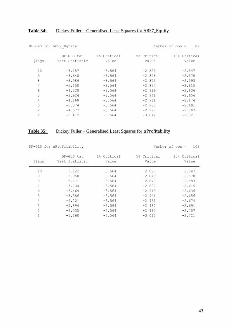
43
Table 34: Dickey Fuller – Generalised Least Squares for ΔBS7_Equity
Table 35: Dickey Fuller – Generalised Least Squares for ΔProfitability
1 -5.412 -3.564 -3.012 -2.721
2 -4.577 -3.564 -2.997 -2.707
3 -5.574 -3.564 -2.980 -2.691
4 -4.168 -3.564 -2.961 -2.674
5 -3.924 -3.564 -2.941 -2.656
6 -4.328 -3.564 -2.919 -2.636
7 -5.150 -3.564 -2.897 -2.615
8 -3.986 -3.564 -2.873 -2.593
9 -3.648 -3.564 -2.848 -2.570
10 -3.187 -3.564 -2.823 -2.547
[lags] Test Statistic Value Value Value
DF-GLS tau 1% Critical 5% Critical 10% Critical
DF-GLS for ΔBS7_Equity Number of obs = 102
1 -5.160 -3.564 -3.012 -2.721
2 -4.535 -3.564 -2.997 -2.707
3 -5.894 -3.564 -2.980 -2.691
4 -4.201 -3.564 -2.961 -2.674
5 -3.586 -3.564 -2.941 -2.656
6 -3.469 -3.564 -2.919 -2.636
7 -3.704 -3.564 -2.897 -2.615
8 -3.171 -3.564 -2.873 -2.593
9 -3.058 -3.564 -2.848 -2.570
10 -3.122 -3.564 -2.823 -2.547
[lags] Test Statistic Value Value Value
DF-GLS tau 1% Critical 5% Critical 10% Critical
DF-GLS for ΔProfitability Number of obs = 102
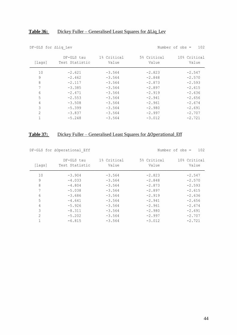
44
Table 36: Dickey Fuller – Generalised Least Squares for ΔLiq_Lev
Table 37: Dickey Fuller – Generalised Least Squares for ΔOperational_Eff
1 -5.248 -3.564 -3.012 -2.721
2 -3.837 -3.564 -2.997 -2.707
3 -5.399 -3.564 -2.980 -2.691
4 -3.508 -3.564 -2.961 -2.674
5 -2.553 -3.564 -2.941 -2.656
6 -2.471 -3.564 -2.919 -2.636
7 -3.385 -3.564 -2.897 -2.615
8 -2.117 -3.564 -2.873 -2.593
9 -2.462 -3.564 -2.848 -2.570
10 -2.621 -3.564 -2.823 -2.547
[lags] Test Statistic Value Value Value
DF-GLS tau 1% Critical 5% Critical 10% Critical
DF-GLS for ΔLiq_Lev Number of obs = 102
1 -6.815 -3.564 -3.012 -2.721
2 -5.202 -3.564 -2.997 -2.707
3 -8.311 -3.564 -2.980 -2.691
4 -5.926 -3.564 -2.961 -2.674
5 -4.641 -3.564 -2.941 -2.656
6 -3.686 -3.564 -2.919 -2.636
7 -5.038 -3.564 -2.897 -2.615
8 -4.804 -3.564 -2.873 -2.593
9 -4.033 -3.564 -2.848 -2.570
10 -3.904 -3.564 -2.823 -2.547
[lags] Test Statistic Value Value Value
DF-GLS tau 1% Critical 5% Critical 10% Critical
DF-GLS for ΔOperational_Eff Number of obs = 102

45
Table 38: Dickey Fuller – Generalised Least Squares for ΔTotal_FScore
Table 39: Dickey Fuller – Generalised Least Squares for ΔGDP
1 -5.422 -3.564 -3.012 -2.721
2 -3.719 -3.564 -2.997 -2.707
3 -5.243 -3.564 -2.980 -2.691
4 -3.839 -3.564 -2.961 -2.674
5 -2.941 -3.564 -2.941 -2.656
6 -2.508 -3.564 -2.919 -2.636
7 -2.840 -3.564 -2.897 -2.615
8 -2.268 -3.564 -2.873 -2.593
9 -2.399 -3.564 -2.848 -2.570
10 -2.637 -3.564 -2.823 -2.547
[lags] Test Statistic Value Value Value
DF-GLS tau 1% Critical 5% Critical 10% Critical
DF-GLS for ΔTotal_FScore Number of obs = 102
1 -4.362 -3.564 -3.012 -2.721
2 -3.802 -3.564 -2.997 -2.707
3 -3.384 -3.564 -2.980 -2.691
4 -3.474 -3.564 -2.961 -2.674
5 -3.164 -3.564 -2.941 -2.656
6 -3.144 -3.564 -2.919 -2.636
7 -3.131 -3.564 -2.897 -2.615
8 -2.614 -3.564 -2.873 -2.593
9 -2.566 -3.564 -2.848 -2.570
10 -3.029 -3.564 -2.823 -2.547
[lags] Test Statistic Value Value Value
DF-GLS tau 1% Critical 5% Critical 10% Critical
DF-GLS for ΔGDP Number of obs = 102

46
Table 40: Dickey Fuller – Generalised Least Squares for Δone_year_ret
Table 41: Dickey Fuller – Generalised Least Squares for ΔF_Revision
1 -3.767 -3.564 -3.012 -2.721
2 -3.877 -3.564 -2.997 -2.707
3 -4.416 -3.564 -2.980 -2.691
4 -2.749 -3.564 -2.961 -2.674
5 -3.462 -3.564 -2.941 -2.656
6 -3.224 -3.564 -2.919 -2.636
7 -3.201 -3.564 -2.897 -2.615
8 -2.515 -3.564 -2.873 -2.593
9 -2.782 -3.564 -2.848 -2.570
10 -3.070 -3.564 -2.823 -2.547
[lags] Test Statistic Value Value Value
DF-GLS tau 1% Critical 5% Critical 10% Critical
DF-GLS for one_year_ret Number of obs = 102
1 -6.287 -3.564 -3.012 -2.721
2 -4.554 -3.564 -2.997 -2.707
3 -4.097 -3.564 -2.980 -2.691
4 -4.274 -3.564 -2.961 -2.674
5 -3.507 -3.564 -2.941 -2.656
6 -3.653 -3.564 -2.919 -2.636
7 -4.018 -3.564 -2.897 -2.615
8 -3.411 -3.564 -2.873 -2.593
9 -3.238 -3.564 -2.848 -2.570
10 -3.320 -3.564 -2.823 -2.547
[lags] Test Statistic Value Value Value
DF-GLS tau 1% Critical 5% Critical 10% Critical
DF-GLS for F_Revision Number of obs = 102
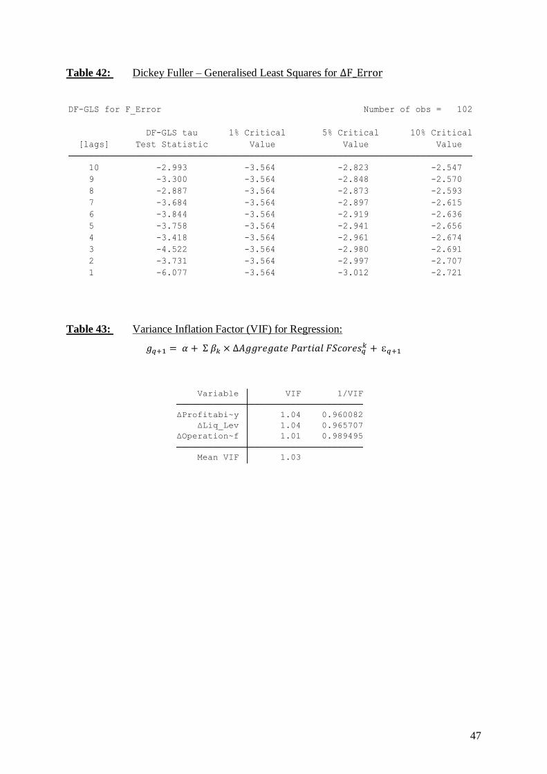
47
Table 42: Dickey Fuller – Generalised Least Squares for ΔF_Error
Table 43: Variance Inflation Factor (VIF) for Regression:
𝑔𝑞+1 = 𝛼 + Σ 𝛽𝑘 × Δ𝐴𝑔𝑔𝑟𝑒𝑔𝑎𝑡𝑒 𝑃𝑎𝑟𝑡𝑖𝑎𝑙 𝐹𝑆𝑐𝑜𝑟𝑒𝑠𝑞𝑘 + 𝑞+1
1 -6.077 -3.564 -3.012 -2.721
2 -3.731 -3.564 -2.997 -2.707
3 -4.522 -3.564 -2.980 -2.691
4 -3.418 -3.564 -2.961 -2.674
5 -3.758 -3.564 -2.941 -2.656
6 -3.844 -3.564 -2.919 -2.636
7 -3.684 -3.564 -2.897 -2.615
8 -2.887 -3.564 -2.873 -2.593
9 -3.300 -3.564 -2.848 -2.570
10 -2.993 -3.564 -2.823 -2.547
[lags] Test Statistic Value Value Value
DF-GLS tau 1% Critical 5% Critical 10% Critical
DF-GLS for F_Error Number of obs = 102
Mean VIF 1.03
ΔOperation~f 1.01 0.989495
ΔLiq_Lev 1.04 0.965707
ΔProfitabi~y 1.04 0.960082
Variable VIF 1/VIF