THE IMPACT OF A PROFESSIONAL SPORTS FRANCHISE

ON COUNTY EMPLOYMENT AND WAGES

John Jasina

Claflin University

School of Business

Kurt Rotthoff

Seton Hall University

Stillman School of Business

Last working version, final version published in:

International Journal of Sport Finance November 2008, Vol. 3, Is. 4

John Jasina can be contacted at: jjasina@claflin.edu, Claflin University, 400 Magnolia St., Orangeburg, SC 29115 and Kurt Rotthoff at: rotthoku@shu.edu, Seton Hall University, JH 621,

400 South Orange Ave, South Orange, NJ 07079. We would like to thank Skip Sauer, Mike

Maloney, Curtis Simon, Chad Turner, Hillary Morgan, and three anonymous referees for the

helpful comments. Any mistakes are ours.

1

ABSTRACT

Stadium boosters have long used the promise of economic development as a

means of gaining public support to finance local sports teams. Past research has

shown little or no impact on employment or income when viewed at the MSA

level. This paper expands the current literature on the economic impact of

professional sports franchises. Following Coates and Humphreys (2003) we look

at employment and wages at the county level using detailed SIC and NAICS

industry codes. We find mixed results on employment within a county, but find a

negative effect on the payrolls within these industries.

2

I. INTRODUCTION

The use of public funds to subsidize privately owned professional sport franchises

has been a hot topic. Across the United States politicians are singing the praises

of sports as a way to develop the economy in their city. Places like Arlington, TX

are supporting the development of new stadiums to lure, or keep, a franchise in

their city. Judith Grant Long (2005) has estimated public subsidies amount to

$177 million per facility while Rappaport and Wilkerson (2001) say more than $6

billion in public funds were spent on stadium and arena construction in the 1990s.

Politicians often claim the local economy will benefit from the creation of new

jobs and higher incomes in order to gain public support for the use of tax dollars

to fund stadium and arena construction.

These claims have lead to research on the actual advantages sports franchises

bring to their city, measured in terms of local economic activity. Over time there

have been many studies on this issue. In earlier works Baade and Dye (1988,

1990) look at retail sales and aggregate income in Metropolitan Statistical Areas

(MSAs). Their 1988 paper finds little support of a link between major league

sports and manufacturing activity, while their 1990 paper finds an insignificant

impact of stadiums on MSA incomes. Baade (1996) looks at a professional sports

team’s ability to create jobs, again failing to find a positive correlation. When

looking at the employment in ten MSAs, Baade and Sanderson (1997) find nine

cities with a significant impact from the presence of a professional sports team.

Interestingly, of the nine significant cities, five were positive and four were

negative.

More recently, Coates and Humphreys (2003) find a small positive, and

significant, effect on the earnings and employment in the amusement and

recreation sector, but they find an offsetting decrease in earnings and employment

in other sectors. This supports the idea that franchises do not create employment

and income, they just cause a shift in consumption, from one sector to another.

Additional studies have attempted to estimate the non-use benefits franchises

bring. For example, when an individual has the ability to watch a local game on

television, read about it in the newspaper, or talk about it with friends, they are

receiving benefits beyond raised income and jobs (Noll and Zimbalist, 1997;

Rapport and Wilkerson, 2001; Johnson, Groothuis, and Whitehead 2001; and

Owen 2006).1

1 Noll and Zimbalist (1997) state that these non-use benefits may be important. However,

Johnson, Groothuis, and Whitehead (2001) find that while the Pittsburgh Penguins generate

substantial civic pride, the value of these public goods falls far short of the cost of the new arena.

3

Many studies have looked at the impact these franchises have had on MSAs,

because MSAs give us a good look at how sports franchises impact economic

activity. However, sports related spending is a small portion of overall spending

in a MSA. For this reason, it may be difficult to pick up the impact of a franchise

when measuring it over such a ‘large area’. This may also be the reason many of

the previous studies find mixed results. This paper expands the current literature

by using county level data, instead of the larger MSA, and by using more detailed

industry codes. This will provide the opportunity, given it exists, to measure the

benefits sports, and new sports arenas, have on economic activity.

The next section discusses the data used. Section three describes the setup of the

model, followed by the presentation of results in section four. Finally, section

five concludes and discusses further research.

II. DATA

Sports related spending represents a small fraction of total spending in an MSA,

so it can be difficult to detect an effect when examining the presence of a sports

franchise and it’s impact on employment. This paper narrows the area of

observation in two ways:

First we use the County Business Pattern dataset, which is produced by the

US Census Bureau, to get county level data from 1986 to 2005.

Secondly we use more detailed, two and four-digit, SIC (Standard

Industrial Classification) employment data.

By narrowing the geographic region of interest, it is anticipated that some impact

from the presence of a sports franchise, should it exist, will be more readily

detected. Using this more defined data set will give us more accuracy in picking

up changes in employment and income related to a sports franchise.

This is contradicted by Carlino and Coulson (2004) who estimate the willingness to pay for an

NFL franchise by looking at rental rates and wages in cities. Their hypothesis is that sports fans

are willing to pay for a team by accepting lower wages and paying higher rental rates. Based on

their results, they conclude that in order to retain an NFL franchise, some subsidies may be justified in large cities. When measuring quality of life, Rappaport and Wilkerson (2001) find that

although residents generally revise the estimates upward (of their willingness to pay) after losing a

football team, only one area allocated considerably more public funding to obtain a new team (or

to try to persuade the old team to come back).

4

Coates and Humphreys (2003 – hereafter C&H) find a small positive effect on

earnings per employee in amusement and recreation, but an offset decrease in

earnings and employment in other sectors. Although they find only one industry

benefits at the cost of other industries, these other industries are thought, by some,

to have a positive benefit from a franchise. The apparel and accessory store

industry is said to benefit because of an increase in foot traffic of visitors of

stadium events. Fans of the local sports teams will also purchase sports related

memorabilia from local stores. If this occurs in stores near new stadiums,

additional spending at these stores will increase retail employment. Employment

in eating and drinking places may also increase due to a new sports team. The

argument is that fans that frequent the stadium will also spend money at local

restaurants and bars. Also, fans not attending the game will seek out bars and

restaurants to watch the events on television. If the claims made in economic

impact studies are correct, then we should be able to observe an increase in

employment and income in these industries after a new franchise moves into the

area (or a decrease as a franchise leaves).

The industries used in this study are areas thought to benefit from the presence of

a sports franchise. We will use apparel and accessory stores (SIC code 56,

NAICS2 code 448), hotels and other lodging (7011, 7211), drinking places (5813,

7224), eating places (5812, 722) and liquor stores (5921, 4453). We will be

looking at employment and wages for all five of these industries. In addition we

will look at the total employment and total wages within the county, for all

industries.

The data include all counties in the US that have, or had, a professional sports

team from 1986-2005. Sports include: baseball (MLB), basketball (NBA),

hockey (NHL), and football (NFL). This means we have information on 58

different counties in the US, many of which have more than one franchise in the

county at any given period of time.3 As an example (Table I) there are 35

counties in the US that have, or had, a professional football team during this time

period, three of which both lost and gained a team over the twenty years included

in our study.

2 The NAICS (North American Industrial Classification System) code has replaced the SIC code, according to the US Censuses Bureau (http://www.census.gov/epcd/www/naics.html), as a more

accurate and standardized way of representing industries. 3 We drop New Orleans (Orleans county) out of the data set, although it is one of the 58. We do

this because of hurricane Katrina causing this county to have extreme abnormalities in the data

that are unrelated to the sporting industry.

5

Table I - NFL Franchises in Dataset:4

County State Team Last or First year with a team*

Alameda CA Raiders Gained Team, 1995

Allegheny PA Steelers

Baltimore MD Ravens Gained Team, 1996

Bergen NJ Giants and Jets

Brown WI Packers

Cook IL Bears

Cuyahoga OH Browns Lost Team, 1995 - Gained Team, 1999

DC Redskins Lost Team, 1996

Dallas TX Cowboys

Davidson TN Titans Gained Team, 1997

Denver CO Broncos

Duval FL Jaguars Gained Team, 1995

Erie NY Bills

Fulton GA Falcons

Hamilton OH Bengals

Harris TX Oilers and Texans Lost Team, 1997 - Gained Team, 2002

Hennepin MN Vikings

Hillsborough FL Buccaneers

Jackson MO Chiefs

King WA Seahawks

Los Angeles CA Raiders Lost Team, 1994

Maricopa AZ Cardinals Gained Team, 1988

Marion IN Colts

Mecklenburg NC Panthers Gained Team, 1995

Norfolk MA Patriots

Miami Dade FL Dolphins

Oakland MI Lions Lost Team, 2001

Orange CA Rams Lost Team, 1994

Orleans LA Saints

Philadelphia PA Eagles

Prince George’s MD Redskins Gained Team, 1997

San Diego CA Chargers

San Francisco CA 49ers

St. Louis MO Cardinals and Rams Lost Team, 1987 - Gained Team, 1995

Wayne MI Lions Gained Team, 2002

* - NFL franchise moves from 1986-2005.

4 A list of all counties can be found in appendix A.

6

We have two different sets of information, county specific data (Table II) on each

of the 58 counties, as well as team specific data (Table III) for each of the

franchises located in these counties. The county data include the employment

within each industry, total payroll in that industry, average wage per employee

(total payroll divided by employees), the number of establishments within that

industry, as well as yearly dummy variables to capture any time trends.

Table II - County Variables:

Variable Description

emp Employment

ap Total Payroll (wages)

qp1 Total First Quarter Payroll (wages)

avgpay Average Wage per Employee (ap/emp)

est Number of Establishments

Y1987-y2005 Yearly Dummy Variables (years 1987-2005)

The team specific data include a dummy variable if a team is present, as well as a

dummy if the stadium used by that team is a multiple use stadium. We also

include the capacity of each stadium (with capacity squared, to capture non-linear

possibilities) and a dummy variable to capture the novelty effect of a new

stadium. To control for this novelty effect, we have dummies set up for both five

and ten years. We also control for entry and exit of teams within five years and

ten years in each sport.

Table III – Sports Related Variables:

Variable* Description

L Dummy variable if a team is present

Lmulti Dummy if L stadium is multi-use

L_capac Capacity of the Stadium

L_capac2 Capacity squared

Lco5 Dummy variable for the opening of a new stadium (5yr)

Lco10 Dummy variable for the opening of a new stadium (10yr)

Lentry5 Five year entry dummies

Lentry10 Ten year entry dummies

Lexit5 Five year exit dummies

Lexit10 Ten year exit dummies

* Where L stands for the league (each MLB, NBA, NHL and NFL)

We have the data to do the opening, entry, and exit variables at both the five and

ten year level. However when using both, we use too many degrees of freedom.

7

We have therefore decided to use the five year dummies in our regressions, but

find no significant differences when regressions are run using both variables

together or either year lag separately.

III. MODEL

In this study, we replicate the C&H model with more specific data described in

the previous section. We use a linear reduced form model; imitating earlier

methodology by using employment, payroll, and average wages for each of the

five different industry codes, as well as for the total employment. Following the

same functional form, we use:

yjit = βj xit + γj zit + μjit

Assuming:

μjit=ejit+vji+ujt

Where t is the year, i is the county and j indexes the three dependent variables of

interest. There are three dependent variables (employment, payroll, and average

wage per employee) each run on the five industry codes as well as the total county

data (18 different regressions). Continuing to follow C&H, we assume that the

dependent variables differ, so that we can use the same explanatory variables, xit

and zit, but are able to estimate different vectors of unknown parameters, βj and γj.

As with their model, the vector of xit captures the general economic climate in

each county over the sample period. This includes the lagged value of the

dependent variable. However, we will use the number of establishments in the

county instead of the growth rate in the population. To control for time trends, or

county trends, we will test the model for the appropriate use of fixed effects or

random effects.

The zit captures sport specific controls: dummies for the four major sports (MLB,

NBA, NHL and NFL) with year dummies for the existence of a team (dummy

equals 0 for no team and equals 1 for having a team, and the counties that

experience a team move have both 0’s and 1’s, while the counties that have a

team throughout the data set will have all 1’s), variables for those counties that

have multi-use stadiums5, as well as capacity and capacity squared (for each

league individually) are all included in this vector. It also includes five year

5 The multi-use variables are statistically significant, however not economically meaningful.

8

dummies for each of the following: opening of a new stadium, the entry of a team,

and the exit of a team.

We assume the μjit follows the same functional form as in C&H. C&H state:

where v is a disturbance specific to dependent variable j in MSA i which persists

throughout the sample period, u is a time t specific disturbance which affects all

areas in the same way, and e is a random shock to dependent variable j in MSA i

at time t which is uncorrelated across dependent variables and MSAs [counties] as

well as over time. Estimated this way, the regression purges the dependent

variable of the effect of national events on each jurisdiction in a given year and

generates an MSA-specific impact.6

We also control for a novelty effect of a new stadium. People find new stadiums

to be a great place to visit, however this does not necessarily mean the impact of a

stadium will have a sustained increase. Coffin (1996) finds the novelty effect of a

new stadium begins to decline in the third year. Because of this, we use a dummy

(example: NFLco5) for the five years after a new stadium is built to make sure we

capture all of the novelty effect. This controls for a short burst in activity a new

stadium creates. We also control for the entry (NFLentry5) or exit (NFLexit5) of

a franchise (in each of the leagues) for the five years after they come or leave,

respectively.

There can be issues in using a lagged dependent variable in the regression; biases

can exist due to its high correlation with the dependent variable. But as shown in

Judson and Owen (1997), this should not affect the independent variables. We

believe it is not a problem because the coefficient of interest is not the lagged

dependent variable; it is the other independent variables which will show any

impact.

IV. RESULTS

In addition to the independent variables we still need to control for variations in

the counties. An omitted variable bias may exist without additional independent

variables including a control for county trends. C&H used year and county

dummies to control for time trends and county trends, while we use year dummy

variables for the time trends and a fixed effects model to control for county

trends. Below (Tables IV, V, and VI) show the regressions using fixed effects.

The FE at the bottom of each regression shows the results of the Hausman test, to

6 From Coates and Humphrey’s 2003 work “The effect of professional sports on earnings and

employment in the service and retail sectors in US cities“, page 182 describing equation 2.

9

see if the Fixed Effects model is a better estimator than a random effects model.

A yes in the FE means that the X2 of the Hausman test is significantly large

enough to reject the null.7

Our test shows that the random effects are inefficient (except Hotel in

employment and Total for both employment and payroll), so fixed effects should

be used. However it is important to note that using fixed effects means that all

counties that have a team throughout the study are essentially dropped from the

regression. Using a fixed effects model takes away our ability to measure any

variable that does not change across time, so if there is an NFL team in a given

county over the whole sample, we cannot estimate the effects of the NFL

(Dummy variable for having a team present) for that county. The benefit of using

this model is that we only test counties which have franchise movement, helping

us answer the question: does a franchise moving into town (or out of town) have

an effect on employment and payroll in these industries? This is exactly what we

need to answer in order to look at the politicians’ claims that these franchises

increase employment and payroll.

Table IV reports the estimated effects on employment within the county from

having a major sports franchise present.

Table IV – Employment:8

Employment

Clothing Drinking Food Hotel Liquor Total

MLB 3085.464 -905.191 14143.1 2543.024 39.198 55770.02

(2.57)* (0.84) (2.43)* (1.05) (0.24) (1.30)

NBA 2360.039 -644.795 2896.93 1358.418 -215.237 -28221.6

(3.57)** (1.10) (0.89) (1.06) (2.20)* (1.21)

NHL -2539.28 -1095.35 3577.842 2941.385 321.911 102174.1

(1.01) (0.48) (0.29) (0.57) (0.93) (1.13)

NFL -7482.31 -5082.85 45854.2 10798.15 -1568.97 -6373.36

(2.19)* (1.67) (2.76)** (1.41) (3.31)** (0.08)

FE Yes N/A Yes Yes N/A N/A

Joint Sig Yes No Yes No Yes No

Absolute value of z-statistics in parentheses

* significant at 5% level; ** significant at 1% level

7 A N/A in the row FE means that the Hausman test was unable to be run. 8 Appendix B shows the full regressions for the Employment Data.

10

When looking at employment, it is shown that the presence of a Major League

Baseball team positively affects the clothing and food industry in terms of

employment. The National Basketball Association is split; they increase

employment in the clothing industry but decrease employment in the liquor

industry. The league that has the most significant impact is the NFL. The NFL

has a negative effect on the clothing and liquor industries while having a positive

impact on the food industry. The NHL has no significant impacts.

Table V reports the estimated effects on payroll within the county from having a

major sports franchise present.

Table V – Payroll:9

Payroll

Clothing Drinking Food Hotel Liquor Total

MLB 23161.03 -30533.2 -41357.2 14463.66 -2858.98 1845916

(0.93) (2.88)** (0.61) (0.23) (0.80) (0.56)

NBA 13275.33 809.057 71407.82 14200.92 807.748 1733267

(0.97) (0.14) (1.89) (0.43) (0.39) (0.97)

NHL 21782.57 -3145.42 125915.3 36508.29 -5903.36 -1996375

(0.42) (0.14) (0.88) (0.28) (0.79) (0.29)

NFL -95482.9 -81503.8 -621858 145047.3 -22100.4 -3081013

(1.35) (2.73)** (3.22)** (0.73) (2.16)* (0.48)

FE Yes Yes N/A No Yes N/A

Joint Sig No Yes Yes No No No

Absolute value of z-statistics in parentheses

* significant at 5% level; ** significant at 1% level

When looking at payroll, the NBA and NHL have no significant impact whereas

both the MLB and the NFL have an impact in some industries. However, all

payroll effects are negative. MLB has a negative effect on the drinking industry

and the NFL has a negative effect on drinking, food, and liquor.

Table VI reports the estimated effects on the average wage per employee within

the county from having a major sports franchise present.

9 Appendix C shows the full regressions for the Payroll Data.

11

Table VI – Average Wages per Employee:10

Average Wage per Employee

Clothing Drinking Food Hotel Liquor Total

MLB 0.413 -1.843 0.349 -0.854 3.239 1.988

(0.27) (1.10) (0.34) (0.30) (0.83) (0.83)

NBA -0.955 1.058 -0.457 0.324 0.21 0.608

(1.13) (1.16) (0.80) (0.22) (0.09) (0.47)

NHL -4.081 1.845 -0.838 -11.124 -2.881 -8.339

(1.26) (0.52) (0.39) (1.86) (0.35) (1.64)

NFL 4.006 -3.569 2.053 2.804 1.83 2.717

(0.92) (0.75) (0.70) (0.31) (0.16) (0.58)

FE Yes Yes Yes Yes N/A Yes

Joint Sig No No No No No No

Absolute value of z-statistics in parentheses

* significant at 5% level; ** significant at 1% level

Looking at the average wage per employee, calculated by dividing the payroll by

the employment in that industry, we find no significant impact by any industry.

There is also no evidence of joint significance in any industry. This shows that

although we find some effect on employment and payroll at the county level, it

has an affect on overall workers (more or less workers in the industry), but not the

individual worker.

Three key findings:

Support of the theory that jobs are not created, there is just movement between

industries.

Employment in the clothing sector is mixed, employment in the liquor

sector decreases, and there is an increase in the food sector.

Payrolls don’t increase, they only decrease.

The presence of franchises have virtually no effect on payrolls, and when

it does have an effect (NFL – drinking, food, and liquor and MLB –

drinking) it is negative.

Total employment and payroll of a county are independent of the existence of a

professional sports franchise.

10 Appendix D shows the full regressions for the Average Wage per Employee.

12

The joint significance (Joint Sig) test shows that, not only do sports

franchises have no impact on the total employment and payroll in a

county, but all sports jointly have no impact on the total county

employment (this is in all industries).

Table VII - Overall Effect:

Employment Payroll Average Wage per

Employee

Positive Negative Positive Negative Positive Negative

Clothing 2 1 0 0 0 0

Drink 0 0 0 2 0 0

Food 2 0 0 1 0 0

Hotel 0 0 0 0 0 0

Liquor 0 2 0 1 0 0

Total 0 0 0 0 0 0

Sum 4 3 0 4 0 0

As seen in Table VII, there are mixed effects in the employment industries from a

franchise moving into (or leaving) a county. This supports the work done by

C&H at the MSA level. However we find only negative effects on payroll and

average wages as a franchise moves into a county, implying there is a positive

effect on payrolls and average wages as a franchise leaves a county.

V. CONCLUSION

Public subsidies for professional sports stadiums are often used as a means to

stimulate economic development in local communities. Economic impact studies,

as well as the politicians pushing them, claim that stadiums will induce job

creation and revenue expansion. Using data on metropolitan statistical areas,

academics find little to support the claims that stadiums help create jobs and

increase the income in the local economy. This paper adds to the current

literature by using detailed county level data to analyze the effect of a stadium on

a smaller area around the stadium.

This study finds that employment within these industries (clothing, drinking,

food, hotel, and liquor) have mixed results when a franchise is present, this is

consistent with Coates and Humphrey’s (2003). However, although most of the

payroll data is insignificant, the coefficients that are significant are all negative.

This also supports Coates and Humphrey’s (2003) findings that real per capita

13

income falls when sports franchises are present. Continued research using this

more detailed data at the county level, over longer periods of time, will bring us

more incite into the true effects of having these franchises present. In addition,

research into the changes in rental rates of the industries when a stadium comes to

town would be information revealing.

14

REFERENCES

Baade, R. A. (1996). Professional sports as catalysts for metropolitan economic

development. Journal of Urban Affairs, 18(1), 1-17.

Baade, R. A. and Dye. R. F. (1988). An analysis of the economic rational for

public subsidization of sports stadiums. The Annals of Regional Sciences,

22(2), 37-47.

Baade, R. A. and Dye, R. F. (1990). The impact of stadiums and professional

sports on metropolitan area development. Growth and Change, 1-14.

Baade, R. A. and Sanderson, A. R. (1997). The employment effect of teams and

sports facilities. Sports, Jobs and Taxes: The Economic Impact of Sports

Teams and Stadiums. Washington, DC: Brookings Institute.

Carlino, G. and Coulson, N. E. (2004). Compensating differentials and the social

benefits of the NFL. Journal of Urban Economics, 56, 25-50.

Coates, D. and Humphreys, B.R. (1999). The growth effects of sport franchises,

stadia and arenas. Journal of Policy Analysis and Management, 18(4),

601-624.

Coates, D. and Humphreys, B. R. (2003). The effect of professional sports on

earnings and employment in the services and retail sectors in US cities.

Regional Science and Urban Economics, 33, 175-198.

D.A. Coffin. (1996). If you build it, will they come? Attendance and new stadium

construction. In: J. Fizel, E. Gustafson and L. Hadley, Editors, Baseball

Economics: Current Research, Praeger, Westport, CT, pp. 33–46.

Judson, R.A. and Owen, A.L. (1997). Estimating Dynamic Panel Data Models: A

Practical Guide for Macroeconomists. fEDS, 1997-3.

Johnson, Bruce K., Peter A. Groothuis and John C. Whitehead. (2001). The Value

of Public Goods Generated by a Major League Sports Team: The CVM

Approach. Journal of Sports Economics 2:1 p. 6-21.

Long, J. G. (2005). Full count: The real cost of public funding for major league

sports facilities. Journal of Sports Economics, 6(2), 119-143.

15

Owen, J. G. The Intangible Benefits of Sports Teams. (2006). Public Finance and

Management 2006. 6(3), 321-345.

Rappaport, Jordan and Wilkerson, Chad. (2001). What Are the Benefits of hosting

a Major League Sports Franchise? Federal Reserve Bank of Kansas City –

Economic Review, First Quarter 2001

16

APPENDIX A

Counties in Dataset

Alameda CA Hamilton OH Oakland MI Allegheny PA Harris TX Oklahoma OK Baltimore MD Hartford CT Orange CA

Bergen NJ Hennepin MN Orange FL

Bernalillo NM Hillsborough FL Orleans LA

Bexar TX Jackson MO Philadelphia PA

Bronx NY Jackson TN Pinellas FL Brown WI King WA Prince George’s MD

Clark NV Los Angeles CA Queens NY

Cobb GA Maricopa AZ Ramsey MN Cook IL Maricopa AZ Sacramento CA Cuyahoga OH Marion IN Salt Lake UT

Cuyahoga OH Marion IN San Diego CA

D C Mecklenburg NC San Francisco CA

Dallas TX Miami Dade FL Santa Clara CA Davidson TN Miami Dade FL Shelby TN Denver CO Milwaukee WI St. Louis MO

Duval FL Montgomery PA Suffolk MA Erie NY Multnomah OR Summit OH

Fairfax VA Nassau NY Tarrant TX

Franklin OH Norfolk MA Wake NC Fulton GA NY NY Wayne MI

Guilford NC Oakland MI

17

APPENDIX B

Employment Regressions

Employment

Clothing Drink Food Hotel Liquor Total

emp emp emp emp emp emp

L.emp 0.647 0.363 0.326 0.686 0.529 0.738

(31.44)** (20.14)** (18.27)** (27.10)** (26.44)** (39.25)**

est 5.34 12.297 16.503 8.617 2.896 5.325

(17.39)** (31.67)** (44.85)** (4.72)** (19.38)** (11.80)**

mlb 3085.464 -905.191 14143.1 2543.024 39.198 55770.02

(2.57)* (0.84) (2.43)* (1.05) (0.24) (1.30)

mlbco5 -106.172 69.455 223.609 215.841 7.234 5937.624

(1.18) (0.86) (0.51) (1.13) (0.59) (1.83)

mlbentry5 272.517 -115.453 -678.183 -271.011 12.585 -82.833

(1.52) (0.71) (0.78) (0.79) (0.52) (0.01)

mlbexit5 0 0 0 0 0 0

(0.00)** (0.00)** (0.00)** (0.00)** (0.00)** (0.00)**

mlbmulti 0 15.5 215.629 597.737 -15.895 30.538

(0.00)** (0.12) (0.31) (2.06)* (0.79) (0.01)

mlb_capac -0.1 0.053 -0.618 -0.086 -0.001 -2.569

(2.30)* (1.36) (2.95)** (0.99) (0.21) (1.66)

mlb_capac2 0 0 0 0 0 0

(1.97)* (1.78) (3.30)** (1.01) (0.39) (1.87)

nba 2360.039 -644.795 2896.93 1358.418 -215.237 -28221.6

(3.57)** (1.10) (0.89) (1.06) (2.20)* (1.21)

nbaco5 23.687 -169.235 -3.81 -125.072 -3.834 816.681

(0.32) (2.53)* (0.01) (0.82) (0.37) (0.31)

nbaentry5 84.971 131.426 419.185 -648.062 41.818 -7153.49

(0.64) (1.10) (0.65) (2.32)* (2.14)* (1.52)

nbaexit5 356.524 12.006 -1774.6 -7.323 0.811 -3456.56

(2.13)* (0.08) (2.15)* (0.02) (0.03) (0.58)

nbamulti 53.839 228.851 1472.227 -366.149 -18.014 4961.555

(0.35) (1.69) (2.01)* (1.18) (0.86) (0.92)

nba_capac -0.254 -0.006 -0.438 -0.09 0.017 2.676

(4.71)** (0.12) (1.57) (0.87) (2.18)* (1.39)

nba_capac2 0 0 0 0 0 0

(5.26)** (1.18) (2.48)* (1.02) (1.89) (1.35)

nhl -2539.28 -1095.35 3577.842 2941.385 321.911 102174.1

(1.01) (0.48) (0.29) (0.57) (0.93) (1.13)

nhlco5 -109.003 -120.385 -1296.08 111.982 -18.9 -91.249

(1.11) (1.36) (2.71)** (0.54) (1.38) (0.03)

nhlentry5 87.993 89.378 833.243 506.567 18.393 -7570.86

(0.82) (0.92) (1.59) (2.15)* (1.26) (1.94)

18

nhlexit5 -108.378 -2.173 382.484 -524.553 -18.494 3583.446

(0.78) (0.02) (0.56) (1.56) (0.98) (0.72)

nhlmulti 0 0 0 0 0 0

(0.00)** (0.00)** (0.00)** (0.00)** (0.00)** (0.00)**

nhl_capac 0.238 0.051 -0.387 -0.287 -0.038 -8.904

(0.91) (0.21) (0.30) (0.54) (1.06) (0.94)

nhl_capac2 0 0 0 0 0 0

(0.87) (0.01) (0.26) (0.41) (1.12) (0.78)

nfl -7482.31 -5082.85 45854.2 10798.15 -1568.97 -6373.36

(2.19)* (1.67) (2.76)** (1.41) (3.31)** (0.08)

nflco5 -14.098 73.054 -314.899 64.358 -10.172 5338.499

(0.13) (0.78) (0.62) (0.26) (0.71) (1.48)

nflentry5 83.733 34.504 248.11 -159.763 22.32 -16782.8

(0.62) (0.29) (0.37) (0.49) (1.21) (3.65)**

nflexit5 -382.468 6.722 -1131.67 -600.314 -32.976 14851.81

(2.60)** (0.05) (1.60) (1.80) (1.60) (2.89)**

nflmulti 251.92 0 0 0 0 0

(1.76) (0.00)** (0.00)** (0.00)** (0.00)** (0.00)**

nfl_capac 0.216 0.166 -1.328 -0.288 0.046 0.139

(2.28)* (1.97)* (2.88)** (1.36) (3.47)** (0.06)

nfl_capac2 0 0 0 0 0 0

(2.51)* (2.27)* (3.08)** (1.26) (3.73)** (0.01)

y1987 0 -769.814 2970.164 -678.919 9.357 0

(0.00)** (7.44)** (5.60)** (2.52)* (0.61) (0.00)**

y1988 -77.506 -584.371 3099.92 -316.954 -0.679 3985.991

(0.74) (5.87)** (5.83)** (1.17) (0.05) (1.11)

y1989 -78.876 -358.386 4385.142 -53.634 -14.851 15635.09

(0.75) (3.67)** (8.09)** (0.20) (1.00) (4.33)**

y1990 -168.259 -299.79 5123.326 89.794 -17.821 9268.983

(1.60) (3.09)** (9.30)** (0.34) (1.20) (2.54)*

y1991 -54.827 -103.603 4249.385 -410.113 -28.455 -10700

(0.52) (1.07) (7.65)** (1.59) (1.95) (2.91)**

y1992 -327.445 -439.825 2145.627 -729.998 -26.951 -11082.5

(3.07)** (4.47)** (4.08)** (2.78)** (1.86) (3.03)**

y1993 93.773 -396.787 1872.285 -324.784 -40.762 -1816.68

(0.88) (4.05)** (3.65)** (1.23) (2.85)** (0.50)

y1994 -36.243 -452.402 1111.894 -685.9 -29.442 -1615.58

(0.33) (4.63)** (2.17)* (2.57)* (2.07)* (0.44)

y1995 67.244 -220.017 3262.807 -259.33 -23.617 11397.52

(0.60) (2.28)* (6.32)** (0.97) (1.69) (3.05)**

y1996 -96.183 -489.725 1692.225 -473.132 -12.716 4953.335

(0.86) (5.02)** (3.37)** (1.79) (0.91) (1.31)

y1997 388.569 -324.454 0 4.389 -21.884 14458.92

(3.36)** (3.34)** (0.00)** (0.02) (1.57) (3.73)**

y1998 671.432 -369.24 -6767.25 -366.982 0 17616.84

19

(6.16)** (3.82)** (10.21)** (1.37) (0.00)** (4.48)**

y1999 126.156 -280.63 1592.089 -165.941 7.939 18600.07

(1.13) (2.93)** (2.63)** (0.60) (0.57) (4.63)**

y2000 587.016 -274.056 1649.823 -195.427 0.435 23419.18

(5.22)** (2.92)** (2.72)** (0.73) (0.03) (5.77)**

y2001 309.034 -145.263 1004.201 -215.64 8.444 14440.23

(2.68)** (1.56) (1.66) (0.81) (0.60) (3.47)**

y2002 57.173 -186.312 657.008 -1614.03 17.515 -20657.4

(0.50) (2.01)* (1.09) (6.09)** (1.24) (4.95)**

y2003 736.304 39.935 407.425 69.838 3.778 878.391

(6.31)** (0.43) (0.69) (0.27) (0.27) (0.22)

y2004 982.749 29.935 -45.1 227.34 5.281 -2848.8

(8.17)** (0.33) (0.08) (0.87) (0.37) (0.69)

y2005 463.996 0 -165.781 0 -26.755 -6946.75

Number of id 57 57 56 56 56 57

Constant -1181.19 -1278.31 -10593.3 1842.471 -48.508 -27460.1

(4.89)** (7.84)** (10.70)** (3.05)** (1.84) (2.51)*

R Squared 0.946 0.622 0.864 0.949 0.769 0.997

Observations 1054 1066 1064 839 1017 1083

Absolute value of z-statistics in parentheses

* significant at 5% level; ** significant at 1% level

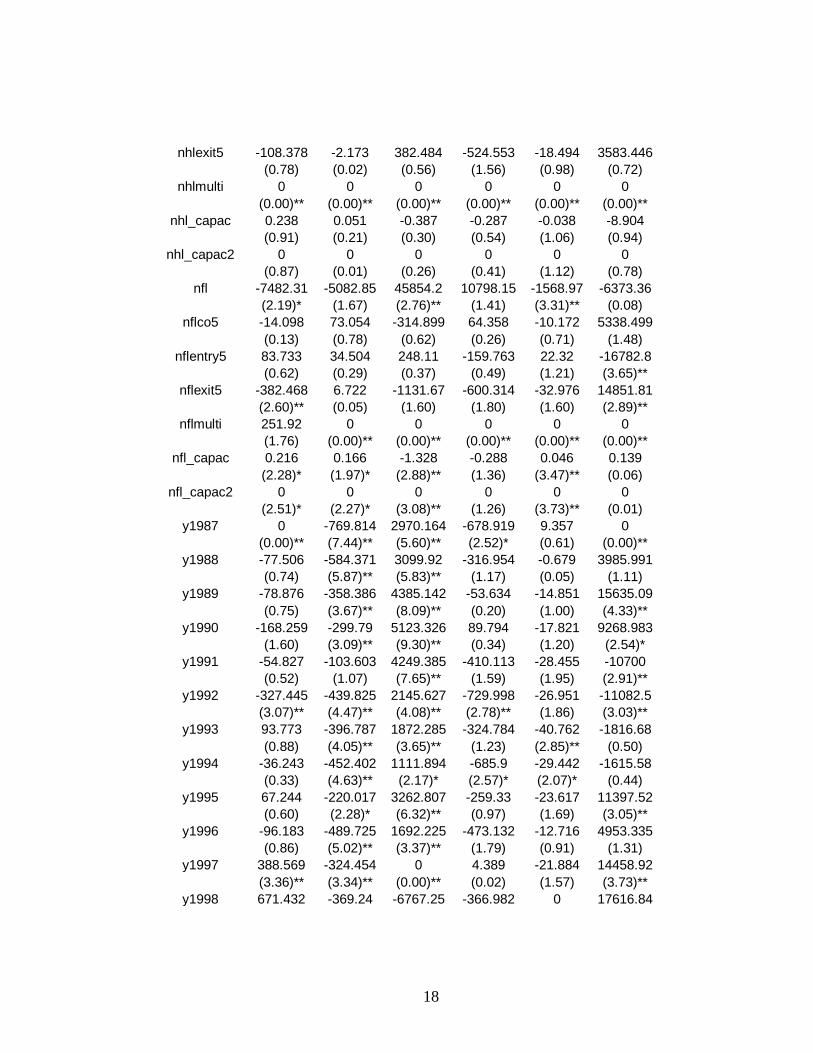
20

APPENDIX C

Payroll Regressions

Payroll

Clothing Drink Food Hotel Liquor Total

ap Ap ap ap ap ap

L.ap 1.016 0.641 0.247 0.985 0.765 0.962

(93.07)** (34.26)** (14.75)** (58.40)** (31.68)** (105.89)**

est 42.734 62.459 203.168 144.445 16.207 167.573

(8.10)** (17.98)** (49.81)** (2.96)** (6.75)** (6.53)**

mlb 23161.03 -30533.2 -41357.2 14463.66 -2858.98 1845916

(0.93) (2.88)** (0.61) (0.23) (0.80) (0.56)

mlbco5 -2827.84 259.297 5260.358 -2702.02 -187.816 -73618.7

(1.52) (0.33) (1.03) (0.55) (0.71) (0.29)

mlbentry5 3124.926 -822.148 7906.574 -225.693 -393.26 -13250.8

(0.84) (0.52) (0.78) (0.03) (0.75) (0.03)

mlbexit5 0 0 0 0 0 0

(0.00)** (0.00)** (0.00)** (0.00)** (0.00)** (0.00)**

mlbmulti 0 -1454.26 14213.6 12381.89 -75.349 250089

(0.00)** (1.15) (1.75) (1.65) (0.17) (0.64)

mlb_capac -0.782 1.333 2.278 -0.461 0.142 -82.097

(0.87) (3.48)** (0.93) (0.21) (1.11) (0.69)

mlb_capac2 0 0 0 0 0 0.001

(0.65) (3.86)** (1.24) (0.17) (1.24) (0.61)

nba 13275.33 809.057 71407.82 14200.92 807.748 1733267

(0.97) (0.14) (1.89) (0.43) (0.39) (0.97)

nbaco5 625.094 -757.95 -2204.07 1306.3 -25.391 167859.4

(0.41) (1.16) (0.53) (0.33) (0.11) (0.83)

nbaentry5 2815.736 1687.855 12687.97 -6028.76 281.616 -56108.6

(1.03) (1.43) (1.69) (0.85) (0.67) (0.16)

nbaexit5 3206.062 905.973 9444.884 -1130.4 377.327 -220104

(0.93) (0.61) (0.99) (0.13) (0.75) (0.47)

nbamulti 4141.72 767.134 -7168.92 -1582.09 318.878 438478.7

(1.31) (0.58) (0.84) (0.20) (0.69) (1.05)

nba_capac -1.202 -0.607 -13.103 -1.205 -0.182 -129.191

(1.08) (1.29) (4.11)** (0.45) (1.07) (0.87)

nba_capac2 0 0 0 0 0 0.002

(0.56) (2.30)* (5.77)** (0.51) (1.56) (0.54)

nhl 21782.57 -3145.42 125915.3 36508.29 -5903.36 -1996375

(0.42) (0.14) (0.88) (0.28) (0.79) (0.29)

nhlco5 687.855 -1136.41 1708.066 401.988 -435.544 -200319

(0.34) (1.31) (0.31) (0.07) (1.47) (0.74)

nhlentry5 -153.942 802.055 -2743.24 10141.41 583.041 -324945

(0.07) (0.84) (0.45) (1.67) (1.85) (1.09)

21

nhlexit5 -539.041 -1001.76 12721.64 -5929.5 -381.639 20739.9

(0.19) (0.81) (1.60) (0.68) (0.94) (0.05)

nhlmulti 0 0 0 0 0 0

(0.00)** (0.00)** (0.00)** (0.00)** (0.00)** (0.00)**

nhl_capac -2.955 -0.276 -15.29 -3.939 0.46 162.92

(0.55) (0.12) (1.02) (0.29) (0.60) (0.22)

nhl_capac2 0 0 0 0 0 -0.003

(0.60) (0.32) (1.14) (0.23) (0.46) (0.16)

nfl -95482.9 -81503.8 -621858 145047.3 -22100.4 -3081013

(1.35) (2.73)** (3.22)** (0.73) (2.16)* (0.48)

nflco5 2984.059 -860.287 -4530.46 1207.863 481.157 232811.4

(1.37) (0.94) (0.77) (0.19) (1.56) (0.84)

nflentry5 -3691.73 2196.606 6718.147 -2247.39 26.815 -663367

(1.31) (1.86) (0.86) (0.27) (0.07) (1.87)

nflexit5 -1403.08 -696.383 -11953.5 -4994.69 -469.846 269112.3

(0.46) (0.54) (1.45) (0.58) (1.05) (0.68)

nflmulti 5076.586 0 0 0 0 0

(1.71) (0.00)** (0.00)** (0.00)** (0.00)** (0.00)**

nfl_capac 2.843 2.373 18.831 -3.929 0.622 82.099

(1.44) (2.86)** (3.51)** (0.72) (2.18)* (0.45)

nfl_capac2 0 0 0 0 0 -0.001

(1.59) (3.05)** (3.83)** (0.65) (2.29)* (0.44)

y1987 0 -8508.28 -39181.8 -5198.58 0 0

(0.00)** (7.97)** (6.14)** (0.81) (0.00)** (0.00)**

y1988 -3629.95 -7565.45 -24696.5 -168.607 489.196 195343.6

(1.68) (7.43)** (3.93)** (0.03) (1.58) (0.70)

y1989 -1505.42 -6679.45 -251.068 1980.04 311.963 99199.55

(0.69) (6.77)** (0.04) (0.31) (1.01) (0.36)

y1990 -2482.9 -6931.96 22194.55 1036.13 110.468 21432.38

(1.14) (7.18)** (3.48)** (0.17) (0.35) (0.08)

y1991 -7265.01 -5026.21 25303.67 -6376.96 374.749 -598902

(3.34)** (5.18)** (3.95)** (1.03) (1.20) (2.14)*

y1992 -4467.43 -6273.68 -1380.07 -8427.48 159.179 -106470

(2.04)* (6.30)** (0.22) (1.36) (0.51) (0.38)

y1993 -5179.52 -5953.9 -6940.96 -2139.86 53.107 -335617

(2.35)* (6.00)** (1.15) (0.35) (0.17) (1.19)

y1994 -2043.09 -6256.9 -4192.76 -6500.86 370.444 -153688

(0.92) (6.35)** (0.70) (1.05) (1.17) (0.54)

y1995 -5124.88 -4832.28 27649.6 -46.58 475.122 469080.4

(2.24)* (5.00)** (4.63)** (0.01) (1.50) (1.62)

y1996 -393.456 -5559.1 23295.26 2281.9 608.266 512220.6

(0.17) (5.67)** (3.99)** (0.38) (1.90) (1.75)

y1997 3978.856 -4741.11 0 4497.529 896.041 578237

(1.65) (4.88)** (0.00)** (0.76) (2.75)** (1.92)

y1998 21057.16 -4080.12 -54678.3 8340.614 1268.863 1231080

22

(9.29)** (4.23)** (7.26)** (1.34) (3.83)** (4.04)**

y1999 2774.697 -3509.69 21848.46 0 1287.581 1057250

(1.18) (3.68)** (3.10)** (0.00)** (3.86)** (3.40)**

y2000 32.193 -2678.24 32403.59 17030.75 1363.952 1989645

(0.01) (2.88)** (4.59)** (2.58)* (4.08)** (6.32)**

y2001 -2387.42 -2191.68 27688.97 -28825.2 1450.337 -129766

(0.99) (2.40)* (3.95)** (4.25)** (4.30)** (0.40)

y2002 -3932.65 -2098.81 25671.2 -25269.9 1616.214 -1780898

(1.63) (2.30)* (3.69)** (3.71)** (4.82)** (5.48)**

y2003 -2302.01 -557.938 21195.47 2642.109 754.593 -525807

(0.93) (0.62) (3.09)** (0.40) (2.21)* (1.63)

y2004 534.956 -337.045 22008.9 14933.36 1608.141 261128.3

(0.21) (0.38) (3.23)** (2.11)* (4.72)** (0.80)

y2005 489.776 0 24224.74 19704.06 2116.831 495463.1

Number of id 57 57 56 56 56 57

Constant -23085.7 (0.00)** -90814 (2.76)** (6.16)** -4056923

(4.54)** -0.09 (7.75)** -0.78 -0.77 (4.65)**

R Squared 0.964 1066.00 0.832 839.00 1017.00 0.988

Observations 1054 0.556 1064 0.976 0.721 1083

Absolute value of z-statistics in parentheses

* significant at 5% level; ** significant at 1% level

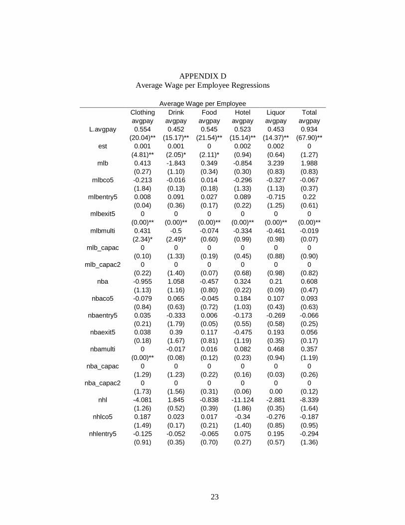
23

APPENDIX D

Average Wage per Employee Regressions

Average Wage per Employee

Clothing Drink Food Hotel Liquor Total

avgpay avgpay avgpay avgpay avgpay avgpay

L.avgpay 0.554 0.452 0.545 0.523 0.453 0.934

(20.04)** (15.17)** (21.54)** (15.14)** (14.37)** (67.90)**

est 0.001 0.001 0 0.002 0.002 0

(4.81)** (2.05)* (2.11)* (0.94) (0.64) (1.27)

mlb 0.413 -1.843 0.349 -0.854 3.239 1.988

(0.27) (1.10) (0.34) (0.30) (0.83) (0.83)

mlbco5 -0.213 -0.016 0.014 -0.296 -0.327 -0.067

(1.84) (0.13) (0.18) (1.33) (1.13) (0.37)

mlbentry5 0.008 0.091 0.027 0.089 -0.715 0.22

(0.04) (0.36) (0.17) (0.22) (1.25) (0.61)

mlbexit5 0 0 0 0 0 0

(0.00)** (0.00)** (0.00)** (0.00)** (0.00)** (0.00)**

mlbmulti 0.431 -0.5 -0.074 -0.334 -0.461 -0.019

(2.34)* (2.49)* (0.60) (0.99) (0.98) (0.07)

mlb_capac 0 0 0 0 0 0

(0.10) (1.33) (0.19) (0.45) (0.88) (0.90)

mlb_capac2 0 0 0 0 0 0

(0.22) (1.40) (0.07) (0.68) (0.98) (0.82)

nba -0.955 1.058 -0.457 0.324 0.21 0.608

(1.13) (1.16) (0.80) (0.22) (0.09) (0.47)

nbaco5 -0.079 0.065 -0.045 0.184 0.107 0.093

(0.84) (0.63) (0.72) (1.03) (0.43) (0.63)

nbaentry5 0.035 -0.333 0.006 -0.173 -0.269 -0.066

(0.21) (1.79) (0.05) (0.55) (0.58) (0.25)

nbaexit5 0.038 0.39 0.117 -0.475 0.193 0.056

(0.18) (1.67) (0.81) (1.19) (0.35) (0.17)

nbamulti 0 -0.017 0.016 0.082 0.468 0.357

(0.00)** (0.08) (0.12) (0.23) (0.94) (1.19)

nba_capac 0 0 0 0 0 0

(1.29) (1.23) (0.22) (0.16) (0.03) (0.26)

nba_capac2 0 0 0 0 0 0

(1.73) (1.56) (0.31) (0.06) 0.00 (0.12)

nhl -4.081 1.845 -0.838 -11.124 -2.881 -8.339

(1.26) (0.52) (0.39) (1.86) (0.35) (1.64)

nhlco5 0.187 0.023 0.017 -0.34 -0.276 -0.187

(1.49) (0.17) (0.21) (1.40) (0.85) (0.95)

nhlentry5 -0.125 -0.052 -0.065 0.075 0.195 -0.294

(0.91) (0.35) (0.70) (0.27) (0.57) (1.36)

24

nhlexit5 0.022 -0.126 0.117 0.242 0.037 -0.074

(0.12) (0.65) (0.97) (0.62) (0.08) (0.27)

nhlmulti 0.837 0 0 0 0 0

(4.24)** (0.00)** (0.00)** (0.00)** (0.00)** (0.00)**

nhl_capac 0 0 0 0.001 0 0.001

(1.17) (0.58) (0.38) (1.80) (0.37) (1.58)

nhl_capac2 0 0 0 0 0 0

(1.07) (0.60) (0.35) (1.70) (0.38) (1.45)

nfl 4.006 -3.569 2.053 2.804 1.83 2.717

(0.92) (0.75) (0.70) (0.31) (0.16) (0.58)

nflco5 0.347 -0.421 0.031 0.083 -0.054 -0.074

(2.58)* (2.89)** (0.35) (0.29) (0.16) (0.37)

nflentry5 -0.466 0.338 -0.24 -0.185 -0.287 -0.14

(2.67)** (1.81) (2.03)* (0.49) (0.66) (0.55)

nflexit5 0.126 0.003 0.028 0.423 -0.828 -0.17

(0.67) (0.01) (0.22) (1.09) (1.70) (0.59)

nflmulti 0 0 0 0 0 0

(0.00)** (0.00)** (0.00)** (0.00)** (0.00)** (0.00)**

nfl_capac 0 0 0 0 0 0

(0.77) (0.67) (0.56) (0.32) (0.30) (0.71)

nfl_capac2 0 0 0 0 0 0

(0.66) (0.60) (0.47) (0.34) (0.42) (0.85)

y1987 0 0 0 0 -5.859 -2.241

(0.00)** (0.00)** (0.00)** (0.00)** (13.62)** (6.21)**

y1988 -0.048 0.48 0.127 0.081 -4.502 -2.026

(0.36) (3.39)** (1.45) (0.36) (10.46)** (5.80)**

y1989 0.397 0.446 0.291 0.307 -4.605 -2.481

(2.93)** (3.08)** (3.31)** (1.39) (11.26)** (7.38)**

y1990 0.565 0.722 0.544 0.507 -4.485 -2.145

(4.10)** (4.82)** (6.07)** (2.25)* (11.18)** (6.52)**

y1991 0.157 0.936 0.775 0.765 -4.001 -2.107

(1.11) (6.07)** (8.40)** (3.36)** (10.15)** (6.60)**

y1992 0.998 0.849 0.817 1.111 -3.979 -1.385

(7.10)** (5.56)** (8.59)** (4.74)** (10.36)** (4.47)**

y1993 0.437 0.663 0.846 1.284 -4.279 -2.307

(2.95)** (4.32)** (8.64)** (5.30)** (11.43)** (7.85)**

y1994 0.997 1.03 0.985 1.475 -3.777 -1.96

(6.77)** (6.72)** (9.75)** (5.84)** (9.96)** (6.79)**

y1995 0.847 1.263 1.108 1.71 -3.362 -1.541

(5.47)** (7.92)** (10.60)** (6.58)** (9.10)** (5.54)**

y1996 1.705 1.424 1.455 2.722 -3.54 -1.228

(10.84)** (8.78)** (13.40)** (10.05)** (9.78)** (4.60)**

y1997 1.805 1.403 1.281 2.497 -2.668 -1.311

(10.27)** (8.33)** (10.84)** (8.38)** (7.30)** (5.14)**

y1998 2.739 1.9 0.762 3.9 -2.408 -0.536

25

(15.65)** (11.05)** (6.06)** (11.92)** (6.81)** (2.19)*

y1999 2.742 2.02 1.406 3.459 -2.078 -0.696

(13.54)** (11.10)** (11.99)** (8.95)** (6.03)** (3.01)**

y2000 2.073 2.557 1.796 4.746 -1.686 0.123

(9.50)** (13.61)** (14.72)** (11.82)** (5.02)** (0.56)

y2001 2.675 2.498 1.699 3.118 -1.616 -1.561

(12.57)** (12.41)** (12.96)** (7.05)** (4.89)** (7.47)**

y2002 2.865 2.539 1.772 4.951 -1.34 -1.587

(12.90)** (12.38)** (13.17)** (11.58)** (4.09)** (7.69)**

y2003 2.408 2.237 1.697 3.884 -1.699 -1.645

(10.28)** (10.71)** (12.34)** (8.58)** (5.22)** (8.05)**

y2004 2.292 2.699 1.915 5.159 -1.113 -0.462

(10.01)** (13.18)** (13.83)** (11.28)** (3.44)** (2.29)*

y2005 3.239 3.527 1.985 5.838 0 0

Number of id 57 57 56 56 56 57

Constant 3.39 3.612 (13.88)** 5.229 10.927 3.714

(9.35)** (11.18)** (13.49)** (8.37)** (13.16)** (4.22)**

R Squared 0.857 0.713 1064.00 0.86 0.631 0.968

Observations 1054 1066 0.865 839 1017 1083

Absolute value of z-statistics in parentheses

* significant at 5% level; ** significant at 1% level