THE IMPACT OF A BUDGET DEFICIT ON TRANSPORT …

THE IMPACT OF A BUDGET DEFICIT ON TRANSPORT INFRASTRUCTURE

INVESTMENT IN SOUTH AFRICA

BY

APHIWE NANTO

A DISSERTATION SUBMITTED IN FULFILMENT OF THE REQUIREMENTS

FOR THE DEGREE

MASTER OF COMMERCE

(TRANSPORT ECONOMICS)

DEPARTMENT OF ECONOMICS

FACULTY OF COMMERCE AND MANAGEMENT

UNIVERSITY OF FORT HARE

SOUTH AFRICA

SUPERVISOR: PROF. R. NCWADI

2013

brought to you by COREView metadata, citation and similar papers at core.ac.uk

provided by South East Academic Libraries System (SEALS)

https://core.ac.uk/display/145043278?utm_source=pdf&utm_medium=banner&utm_campaign=pdf-decoration-v1

i

ABSTRACT

Persistent government budget deficits and government debt have become major concerns in

both developed and developing countries. This study investigates the impact of a budget

deficit on transport infrastructure investment in South Africa. Quarterly time series data,

covering the period 1990q1- 2009q4, was used in this project. The study tests for stationarity

using the Augmented Dickey- Fuller and Phillips Perron; it tests for cointegration using the

Johansen (1991, 1995) methodology. A vector error correction model is used as an estimation

technique. The results of this study show that a budget deficit has a negative impact on

transport infrastructure investment in South Africa.

Keywords: Budget deficit, transport infrastructure investment, VECM, South Africa.

ii

DECLARATION

I, the undersigned, Aphiwe Nanto, hereby declare that this dissertation is my own original

work and that all sources have been accurately reported, acknowledged and referenced.

Moreover, I declare that this document has not previously been submitted at any university

for a similar or any other academic qualification.

Signature …………………………

Date ………/………/………….

iii

ACKNOWLEDGEMENTS

Firstly, I thank my savior the Lord Jesus Christ for his love and strength that he has given me

to make all things possible. Secondly, I thank the National Department of Transport and the

Govan Mbeki foundation for their financial assistance; none of this would have been possible

without your support. I also express my sincere gratitude to my supervisor, Prof. R. Ncwadi,

for his unlimited advice, encouragement and guidance. Finally, I thank my family and

friends who gave me the much needed words of encouragement and advice throughout the

years, it is highly appreciated.

iv

DEDICATION

This thesis is dedicated to my parents, my brothers and my daughter.

v

LIST OF ACRONYMS

ADF: Augmented Dickey Fuller

ARDL: Auto regression distribution lags

AIC: Akaike Information Criterion

ASGISA: Accelerated Shared Growth Initiative for South Africa

BBBEE: Broad Based Black Economic Empowerment

CGC: Classical Growth Cycles

CPI: Consumer Price Index

DF: Dickey Fuller

DTI: Department of Trade and Industry

ECM: Error Correction Model

FDI: Foreign Direct Investment

FPE: Final Prediction Error

GDP: Gross domestic Product

GEAR: Growth, Employment and Redistribution

GFSY: Government Financial Statistics Yearbook

HQ: Hannan-Quinn

IMF: International Monetary Fund

IRF: Impulse Response Functions

JB: Jarque- Bera

KPSS: Kwiatkowski Phillips Schmidt Shin

LM: Lagrange Multiplier

LR: Likelihood Ratio

MTEF: Macro Transport Infrastructure Forum

NEER: Nominal Effective Exchange Rate

NGP: New Growth Path

OECD: Organisation for Economic Co-operation and Development

OLG: Overlapping Generations

OLS: Ordinary Least Squares

PIMS: Political Information and Monitoring Services

PP: Phillips-Perron

R&D: Research and Development

RDP: Reconstruction and Development Programme

vi

RGDP: Real Gross Domestic Product

SAIIA: South African Institute of International Affairs

SARB: South African Reserve Bank

SC: Schwarz Criterion

STATSSA: Statistics South Africa

SUR: Seemingly Unrelated Regression

TII: Transport Infrastructure Investment

TVP-VAR: Time Varying Parameter -Vector Auto Regression

UNCTAD: United Nations Conference on Trade and Development

US: United States

VAR: Vector Auto regression

VECM: Vector Error Correction Model

vii

Table of Contents

ABSTRACT ............................................................................................................................................. i

DECLARATION .................................................................................................................................... ii

ACKNOWLEDGEMENTS ................................................................................................................... iii

DEDICATION ....................................................................................................................................... iv

LIST OF ACRONYMS .......................................................................................................................... v

LIST OF TABLES .................................................................................................................................. x

LIST OF FIGURES ............................................................................................................................... xi

CHAPTER ONE ................................................................................................................................... 1

INTRODUCTION ................................................................................................................................. 1

1.1 Background and Problem Statement ............................................................................................. 1

1.2 Objectives of the study .................................................................................................................. 3

1.3 Hypothesis of the study ................................................................................................................. 4

1.4 Significance of the study ............................................................................................................... 4

1.5 Organisation of the study .............................................................................................................. 4

CHAPTER TWO .................................................................................................................................. 5

LITERATURE REVIEW .................................................................................................................... 5

2.1 Introduction ................................................................................................................................... 5

2.2 Theoretical Literature .................................................................................................................... 5

2.2.1 Harrod-Domar Model ................................................................................................................ 5

2.2.2 Robert Solow Model .................................................................................................................. 6

2.2.2.1 Limitations of the neo-classical growth model ....................................................................... 8

2.2.3 Endogenous Growth Model ....................................................................................................... 9

2.2.3.1 The Lucas Endogenous Growth Model ................................................................................ 10

2.2.3.2 The Romer Model of Endogenous Growth ........................................................................... 11

2.2.3.3 Limitations of the endogenous growth model ....................................................................... 13

2.2.4 Assessment of the Theories...................................................................................................... 13

2.3 Empirical Literature .................................................................................................................... 14

2.3.1 Empirical Evidence from Developed Countries ...................................................................... 14

2.3.2 Empirical Evidence from Developing Countries ..................................................................... 22

2.3.3 Empirical Evidence from South Africa .................................................................................... 29

2.4 Conclusion .................................................................................................................................. 34

CHAPTER THREE ............................................................................................................................ 36

viii

AN OVERVIEW OF THE SOUTH AFRICAN BUDGET DEFICIT AND TRANSPORT

INFRASTRUCTURE INVESTMENT ............................................................................................. 36

3. 1 Introduction ................................................................................................................................ 36

3.2 Historical overview ..................................................................................................................... 36

3.2.1 South African Public Transport Infrastructure Investment 1980-2011 .................................... 37

3.3 Government Revenue 1980-2011 ............................................................................................... 39

3.4 Government Expenditure 1980-2011 .......................................................................................... 41

3.5 Budget Deficit/Surplus 1980-2011 ............................................................................................. 45

3.6 Foreign Direct Investment 1980-2011 ........................................................................................ 47

3.7 Real Gross Domestic Product 1980-2011 ................................................................................... 49

3.8 Conclusion .................................................................................................................................. 52

CHAPTER FOUR ............................................................................................................................... 53

RESEARCH METHODOLOGY ...................................................................................................... 53

4.1 Introduction ................................................................................................................................. 53

4.2 Model specifications ................................................................................................................... 53

4.3 Definition of the variables and data sources ............................................................................... 54

4.4 Expected Priori ............................................................................................................................ 54

4.5 Estimation Techniques ................................................................................................................ 55

4.5.1 Testing for Stationarity/Unit Root ........................................................................................... 55

4.5.2 The Augmented Dickey–Fuller test and Phillips Perron test ................................................... 56

4.5.3 Cointegration and vector error correlation modeling (VECM) ................................................ 57

4.5.4 Diagnostic Tests ....................................................................................................................... 60

4.5.4.1 Autocorrelation LM Test ...................................................................................................... 61

4.5.4.2 Heteroscedasticity test........................................................................................................... 61

4.5.4.3 Residual normality test.......................................................................................................... 61

4.5.5 Impulse response and variance decomposition ........................................................................ 61

4.5.5.1 Impulse response ................................................................................................................... 62

4.5.5.2 Variance Decomposition ....................................................................................................... 62

4.6 Conclusion .................................................................................................................................. 63

CHAPTER FIVE ................................................................................................................................ 64

PRESENTATION OF EMPIRICAL RESULTS ............................................................................. 64

5.1 Introduction ................................................................................................................................. 64

5.2 Stationarity/unit root test ............................................................................................................. 64

5.3 Cointegration............................................................................................................................... 70

ix

5.4 Vector Error Correction Model and the long run relationship .................................................... 74

5.4 Diagnostic Tests .......................................................................................................................... 76

5.5 Impulse response and Variance decomposition .......................................................................... 77

5.6 Variance Decomposition ............................................................................................................. 78

5.7 Conclusion .................................................................................................................................. 80

CHAPTER SIX ................................................................................................................................... 81

SUMMARY OF THE MAIN FINDINGS, CONCLUSIONS, IMPLICATIONS AND

RECOMMENDATIONS .................................................................................................................... 81

6.1 Summary of the study and conclusions ....................................................................................... 81

6.2 Conclusions ................................................................................................................................. 82

6.3 Recommendations ....................................................................................................................... 82

6.4 Delimitations and recommendations for future research ............................................................ 82

REFERENCES .................................................................................................................................... 83

APPENDIX .......................................................................................................................................... 92

Data used in the regression analysis ..................................................................................................... 92

x

LIST OF TABLES

Table 2.1: Summary of selected empirical literature on the budget deficit and transport

infrastructure investment……………………………………………………………………..33

Table 5.1: Unit root/Stationarity Tests……………………………………………………….68

Table 5.2: Phillips-Perron……………………………………………...…………………….70

Table 5.3: Lag Length Criteria……………………………………………………………….72

Table 5.4: Johansen cointegration rank test results………………………………………….73

Table 5.5: Results of both the Long run and Short run Relationship………………………..75

Table 5.6: Results of the Diagnostic Tests…………………………………………………...77

Table 5.7: Variance Decomposition………………………………………………………….80

xi

LIST OF FIGURES

Figure 2.1: Solow Growth Model……………………………………………………………..7

Figure 3.1: Trends in Transport Infrastructure Investment (1980-2011)..…………………...38

Figure 3.2: Trends in Government Revenue (1980-2011)…………………………………...40

Figure 3.3: Trends in Government Expenditure (1980-2011)……………………………….44

Figure 3.4: Trends in the budget deficit/surplus (1980-2011)………………………….…...46

Figure 3.5: Trends in foreign direct investment (1980-2011)………………………………..48

Figure 3.6: Trends in RGDP (1980-2011)…………………………………………………...51

Figure 5.1: Plots of all variables in logarithm form 1990q1-2009q4………………………...66

Figure 5.2: Plots of all variables after differencing 1990q1-2009q4………………………...67

Figure 5.3: Johansen Cointegration Vector…………………………………………………..74

Figure 5.4: Impulse Response………………………………………………………………..78

1

CHAPTER ONE

INTRODUCTION

1.1 Background and Problem Statement

The term ‘budget deficit’ is described as the negative budget surplus whereby government

expenditure exceeds government revenue. Budget revenue includes three important

components, which are: tax revenue, tax exempt revenue and private revenues. The most

important component of the budget revenue is tax revenue. However, budget expenditure

involves four important elements, which are: current expenditure, investment expenditure,

real expenditure and transfer payments (Mwakalikamo, 2011). Current expenditure is the

kind of expenditure related to nondurable goods and services like the payment of wages and

salaries, and it is used for short term expenses. Investment expenditure is related to

investment and capital development, such as the construction of infrastructure and purchasing

of capital goods like tractors and other machines for production (Mwakalikamo, 2011).

Transfer payment includes grants and subsidies which have an indirect impact to the GDP. If

the budget expenditure exceeds budget revenue, which are both important components of the

budget, then it is stated to be a budget deficit.

Persistent government budget deficits and computing government debt have become major

concerns in both developed and developing countries. Extensive theoretical and empirical

literature has been developed to examine the relationship between budget deficits and

macroeconomic variables (Akinbobola and Oladipo, 2011). The monetarists share the view

that fiscal deficits are harmful to an economy. While some of the increases in the deficits

have been associated with declining tax revenue, resulting from the recession, others relate to

the increase in debt service payments on public debt. The development of a budget deficit is

often traced to the Keynesian inspired expenditure-led growth theory of the 1970s (Olomola

and Olagungu, 2004). Most countries of the world adopted the theory that the government has

to spend more in order to stimulate economic growth. However, its consequences on

macroeconomic variables cannot be underestimated in most countries of the world.

The South African government recognises the importance of transport infrastructure in

economic growth in South Africa. In South Africa, the improvement in public transport

infrastructure has served to link undeveloped and developed regions, such as towns and rural

2

areas, and it has been seen as the most valuable policy tool because it acts as a stimulus

during economic downturns (Negota, 2001). The improved transport infrastructure has also

improved trade, to a large extent, since goods can now be delivered without any transport

infrastructure complications (Negota, 2001). Public transport infrastructure investment in the

form of seaports, airports, rail and roads causes South Africa to move towards a sustained and

growing development (Fourie, 2006). This enables all South Africans, especially the poor, to

enjoy greater access to economic empowerment through job creation.

The Minister of Finance, Gordhan, in his budget speech stated that South Africa’s investment

in infrastructure gives impetus to growth in the economy (National Treasury, 2012). An

improvement in economic growth contributes towards the reduction of inequality, poverty

and the creation of decent work for people, especially for those who are not skilled (National

Treasury, 2012). In this regard, the New Growth Path which is currently a South African

macroeconomic strategy creates a way of making the South African economy more

developed and equitable for sustained growth. This strategy encourages stronger investments

in infrastructure, by both the public and private sectors, in order for the country to create the

necessary employment opportunities and at the same time reduce poverty.

Given these objectives of the government to stimulate the economy towards a higher growth

path, there are two primary instruments, amongst others, that a country can use, namely:

fiscal policy and monetary policies. A monetary policy is used mainly to regulate money

supply through interest rates (Mollentze & Van der Merwe, 2010). A fiscal policy on the

other hand, deals with government revenue through tax and expenditure (Nattrass, 2000 and

Ajam and Aron, 2007).

A budget is considered a useful tool of control utilised by companies. It can help set

developmental policies in the country. Budget is a record of the earning and spending of an

organization. When the actual expenditures are in conformity with the planned expenditure,

then planning becomes useful for that unit. Budget can either be a deficit or surplus. A budget

deficit results in situations where the expenditures of the country exceed its revenues, earned

from taxes and other sources. According to Sill (2005), the expenditure of an entity, which

exceeds its earning or income, has been termed a budget deficit. In the absence of financing

from external sources the deficit is carried forward to the next financial year. The deficit can

be a result of delays in the collection of revenues i.e. sales, taxes or other sources of revenues.

Budget revenues decrease due to erosion of the tax base, while expenditures most often rise

3

due to an increase in transfers to the population such as unemployment benefits, social

welfare, etc. (Anušić , 1994). The country entered a recession in 2008 with the government

already spending more than it was taking in tax. However, in any recession, the budget deficit

increases because of the automatic stabilizers that kick in where tax receipts fall and welfare

spending increases. That deficit will not last longer; it will change as soon as the country

experiences increasing returns in the economy.

South Africa reported a government budget deficit equal to 4.80 percent of the country's

Gross Domestic Product in 2011 (National Treasury, 1995). During this period 1989 until

2011, South Africa’s Government Budget averaged -3.03 percent of GDP reaching an all-

time high of 0.90 percent of GDP in December 2007 and a record low of -7.40 percent of

GDP in December 1992. Government Budget is an itemized accounting of the payments

received by government (taxes and other fees) and the payments made by government

(purchases and transfer payments).

Given this scenario of a budget deficit, if not funded by foreign aid and/or increased taxes,

the government may not invest in infrastructure. A lack of infrastructural investment may

lead to a decline in growth as well as job opportunities. However, given these large figures of

a budget deficit on GDP, the question at hand is: does the budget deficit have an effect on

infrastructure investments? How has the budget deficit affected the infrastructure investment

over the years, both in the long and short run? Lastly, what policy recommendations could be

implemented to reduce budget deficits?

1.2 Objectives of the study

The primary objective of this study is to investigate the impact of a budget deficit on public

transport infrastructure investment in South Africa. This broad objective is explored through

the following sub objectives:

To review the trends of both public transport infrastructure investments and budget deficit

from 1990-2009.

To investigate the short run and the long run response of the public transport

infrastructure investment to changes in the budget deficit from the period 1990-2009.

To make policy conclusions and recommendations based on the findings.

4

1.3 Hypothesis of the study

H0: Government budget deficit has a significant negative relationship with transport

infrastructure investment in South Africa.

HA : Government budget deficit does not have a significant negative relationship with

transport infrastructure investment in South Africa.

1.4 Significance of the study

The relationship between the budget deficits on transport infrastructure investment has

attracted a vast amount of literature from both theoretical and empirical fronts in recent years.

Many researchers investigated the relationship between the two, but they have reached

conflicting results. There is still a debate as to whether there is a positive relationship or a

negative relationship, if any, between budget deficit and transport infrastructure investment.

Therefore, this study seeks to fill in that gap by examining the relationship between the two

in South Africa.

1.5 Organisation of the study

Following this introduction, Chapter two reviews both the theoretical and empirical literature

pertaining to the relationship between public transport infrastructure investment and budget

deficit. The chapter made use of the following theories: the Harrod-Domar growth theory;

Robert Solow’s theory and the Endogenous Growth model. The empirical evidence

conducted was from developed and developing countries as well as South Africa specifically.

Chapter three provides an overview of trends in the relationship between public transport

infrastructure investment and budget deficit in South Africa. Chapter four discusses the

methodology and sources of data used in this study. Chapter five estimates the regression

model and interprets the results. Chapter six presents a summary of the study and policy

recommendations. The last chapter points out some limitations associated with the study.

5

CHAPTER TWO

LITERATURE REVIEW

2.1 Introduction

The purpose of this chapter is to explore the various theories of infrastructure investment.

The Harrod-Domar growth theory, Robert Solow’s theory and the Endogenous growth theory

are discussed in this chapter. These theories are important in that they provide the

determinants and fundamental dynamics of infrastructure investment and economic growth.

This chapter is divided into three sections. The first section presents growth theories. The

second section deals with the empirical literature on infrastructure investment and budget

deficit from developed, developing countries and from South Africa. The last section

provides the concluding remarks of this chapter.

2.2 Theoretical Literature

This section is aimed at investigating the determinants of infrastructure investments.

Traditional theories of infrastructure investment, namely; the Harrod-Domar growth theory,

Robert Solow’s theory and Endogenous Growth Models are discussed herein.

2.2.1 Harrod-Domar Model

The Harrod-Domar model stipulates that growth depends on the quality of labour and

investment leads to capital accumulation which later affects the economic growth of a

country (Jones, 2013). This theory has the following assumptions:

1. Output is a function of capital stock i.e.

Y= f (K)

Where Y = Gross Domestic Product and K = Level of Capital Stock

2. The marginal product of capital is constant. This means that marginal and average products

of capital are equal.

3. The product of the savings rate and output equals investment.

sY= S= I

4. The change in the capital stock is equal to investment less depreciation of the capital stock.

6

ΔK= I- δ K

This theory states that in order for the country to grow it solely depends on government

expenditure on investments and savings. The development of a country includes the rate of

output growth solely the rate of infrastructure investment being made in which the

government has enough capital. The main strength of this theory is that the absence of the

economic shocks predicts economic growth in the short run.

2.2.2 Robert Solow Model

The neoclassical growth theory was developed by Robert Solow (1956), a prominent

economist of the twentieth century (Uwasu, 2006). In a nutshell, the Solow model predicted

that a country may experience growth accelerations and growth slowdowns. This model

consists of both a supply and demand side, but it focuses primarily on the supply side. With

reference to this study, this means that it focuses on government expenditures that tend to

have an effect on the public transport infrastructure investment which later affects the

economic growth of a country.

The Solow model states that an increase in the labour supply results in a larger output. This

can only happen if a lot of people take part in a country’s production (for example, if those

who are not part of the labour force start working); when the transport infrastructure takes

place, real output increases. Solow stated that a productivity increase can, for example, take

place when investments in equipment like computers and machinery reduce labour hours.

Productivity increases explain the increase in output that cannot be explained by labour and

capital (inputs), called the productivity of an input, and is affected by a lot of factors.

According to this model, the productivity of an input is affected by technological factors such

as differences in capital per worker and differences in knowledge (Burda and Wyplosz,

2001).

The theory starts with a simplified assumption that there is no technological progress in the

economy; that is, output is a function of the capital-labour ratio and is expressed as follows,

Y= f (K)………………………………………………………………………………….…..2.1

Y = output per head

K = capital per head

The Solow growth model is illustrated in Figure 2.1 below.

7

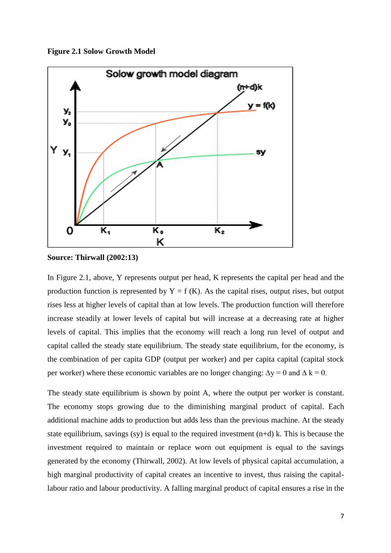
Figure 2.1 Solow Growth Model

Source: Thirwall (2002:13)

In Figure 2.1, above, Y represents output per head, K represents the capital per head and the

production function is represented by Y = f (K). As the capital rises, output rises, but output

rises less at higher levels of capital than at low levels. The production function will therefore

increase steadily at lower levels of capital but will increase at a decreasing rate at higher

levels of capital. This implies that the economy will reach a long run level of output and

capital called the steady state equilibrium. The steady state equilibrium, for the economy, is

the combination of per capita GDP (output per worker) and per capita capital (capital stock

per worker) where these economic variables are no longer changing: ∆y = 0 and ∆ k = 0.

The steady state equilibrium is shown by point A, where the output per worker is constant.

The economy stops growing due to the diminishing marginal product of capital. Each

additional machine adds to production but adds less than the previous machine. At the steady

state equilibrium, savings (sy) is equal to the required investment (n+d) k. This is because the

investment required to maintain or replace worn out equipment is equal to the savings

generated by the economy (Thirwall, 2002). At low levels of physical capital accumulation, a

high marginal productivity of capital creates an incentive to invest, thus raising the capital-

labour ratio and labour productivity. A falling marginal product of capital ensures a rise in the

http://en.wikipedia.org/wiki/File:Solow_growth_model1.png

8

capital-output ratio and a declining incentive to invest until a point is reached at which the

full savings (and hence investment) generated by the economy are employed in order to

supply new labour hours entering the workforce with the same capital intensity as existing

previous labour hours available for production.

The only way for the economy to grow or move from the steady state equilibrium is for the

economy to raise its savings level and maintain a lower labour force growth rate. This can

only happen if savings have risen relative to investment requirements and therefore more is

saved than required to maintain the capital per head constant. This higher savings rate implies

that there will be an incentive to invest, thus increasing the capital-labour ratio and labour

productivity. A high population growth rate leads to a decline in labour productivity

(Thirwall, 2002). A lower growth rate of the labour force allows the use of investment for the

purposes of capital deepening rather than capital widening; again, the consequence is a rising

capital-labour ratio and higher labour productivity. Both changes in the savings rate and

changes in the growth rate of the labour force result in a temporary change in the growth rate

of output as the economy moves towards a new steady state defined by the new savings rate

and labour force growth rate. In a steady state the natural growth rate of the economy would

again prevail (Fedderke & Simkins, 2006). With constant-returns-to-scale production, in the

short run, savings tend to increase the growth rate of output but they do not affect the growth

rate of output in the long run. The implication here is that a higher savings rate initially

increases output or growth but the economy will reach new steady state equilibrium in the

long run.

2.2.2.1 Limitations of the neo-classical growth model

The neo-classical growth model assumes that economies reach long run steady state

equilibrium and the only way for the economy to grow is through technological progress. It

however leaves the determinants or sources of this exogenous variable unexplained. The

model assumes that in the absence of shocks or technological change all economies will

diverge to zero growth. Rising per capita incomes are only a temporary phenomenon

resulting from a change in technology. Any increase in per capita income that cannot be

attributed to labour or capital is ascribed to what is known as the Solow residual. In his

empirical studies, Solow showed that approximately 50 percent of historical growth in

industrialised nations is attributed to the residual (Fedderke & Simkins, 2006). However, it is

impossible to analyse the determinants of technological advances because it is completely

independent (exogenous) of the decisions of economic agents. Another weakness of the

9

Solow growth model is that it fails to explain large differences in residuals across different

countries. The conception that poor countries will eventually catch up with developed

countries, if technological progress is the same, is not effective if there is no explanation of

the determinants of these technological advances (Fedderke & Simkins, 2006). In view of the

weaknesses of the Solow growth model, the new growth theory (endogenous) emerged;

hence, it is discussed in the next sub section.

2.2.3 Endogenous Growth Model

The main purpose of the endogenous growth model is to explain the existence of increasing

returns to scale and contradictory long term growth patterns. The endogenous growth theory

was formed by (Romer, 1986) and (Lucas, 1988). The endogenous growth model outlines

how human capital development as well as research and development (R&D) contribute to

long run economic growth. The endogenous growth model is based on two approaches taken

by the (Romer, 1986) and (Lucas, 1988) models. The theory assumes that there are positive

externalities associated with human capital formation (education and training, for example)

and research and development that prevent marginal product from declining (Thirwall, 2002).

The theory begins with the assumption that there are constant returns in production.

The endogenous growth theory is an extension of the Solow growth model, expressed as

follows:

Y = AK…………………………………………………………………………………..…2.2

Where Y = output

A = total factor productivity (technology)

K = physical and human capital

Equation 2.2 shows that output is proportional to capital. Total factor productivity represents

the marginal product of capital which is constant. The above formula of the endogenous

growth theory proposes that there is no decreasing marginal product of capital and

endogenises technological progress. Therefore, the production function has a constant

marginal product of capital. To prevent the decrease of marginal product of capital it was

proposed that the concept of capital be increased to include human capital (Lucas, 1988). The

concept of human capital, as outlined by Lucas (1988), is explained in the next subsection.

10

2.2.3.1 The Lucas Endogenous Growth Model

The Lucas (1986) approach of endogenous growth introduces the concept of human capital as

opposed to physical labour in the production function. Human capital refers to the knowledge

accumulation or skills gained by workers through learning by doing. The Lucas (1986) model

states that the growth rate of the economy will be determined by the rate of growth of human

capital creation. The Lucas (1986) model of endogenous growth is expressed as follows:

Y = AF (Kα, H

1-α)………………………………………………………………………….2.3

Where: Y = output

A = total factor productivity

K = capital

H= human capital

α and 1-α = output elasticities of the factor inputs. (α and 1-α=1).

Equation 2.3 above illustrates human capital as a component of the production function.

Capital not decreasing and human capital displaying positive externalities, such as education

and training, enables the economy to reach long run economic growth (Todaro and Smith,

2009). Firms and consumers invest in human capital by gaining knowledge. All inputs of the

production function can thus be accumulated. The growth of capital generates new

knowledge about production in the economy as a whole. Growth is then created by assuming

that the motivation to invest in human capital is non-decreasing in human capital (Todaro and

Smith, 2009). The Lucas model of endogenous growth suggests a production function of

human capital which has constant returns to scale in human capital but with the possibility of

increasing returns to scale. Hence, the marginal product of human capital that determines the

incentive to invest in knowledge accumulation is constant. The Lucas model assumes that

human capital relates to the skills and experience gained by the labour force. Investment in

human capital has a positive impact on the growth process. The second approach to

endogenous growth, by Romer (1986, 1990), is discussed in the ensuing subsection.

11

2.2.3.2 The Romer Model of Endogenous Growth

The second aspect of the new endogenous growth theory is in line with research and

development (R&D). The path that a country could take in order to not experience

diminishing returns in the long run would be technological progress. Spending on research

and development (R&D) is considered an investment in knowledge that translates into new

technologies as well as using the resources of physical and human capital that are already in

existence more efficiently. Romer (1986) focuses on research and development as an

important tool to knowledge accumulation. The model adds R&D to the original production

function. This is expressed as follows:

Y = A (R) f (Ri, Ki, Li)............................................................................................................2.4

Where: Y = output

A = total factor productivity

Ki = capital

Li = labour

Ri = stock of results from expenditure on R&D in firm i and where spill over from private

research efforts lead to improvements in the public stock of knowledge.

Equation 2.4, above, shows an augmented production function that includes R&D. In this

model, output is not only a function of capital and labour but also R&D efforts by firms.

Economies of scale are external to firms as technology will move across to other firms

resulting in an improvement in public knowledge. The Romer model of endogenous growth

through technological progress has characteristics of a public good, which states that it is

non-rivalry and partially-excludable. The creation of new knowledge by one firm is assumed

to have a positive external effect on the production possibilities of other firms because

knowledge cannot be perfectly patented or kept secret. With spill-over effects, knowledge

production is an inadvertent side-product of all production and investment activity, and

would take place whether firms wish to undertake it or not, as long as they are engaged in

their standard productive activity (Fedderke & Simkins, 2006). The marginal cost of using

new knowledge is assumed to be zero or close to zero. The low cost of using existing

knowledge is also assumed to lower the cost of producing new knowledge, this results in

dynamic scale economies in knowledge accumulation.

12

The effect of knowledge spill-over is to ensure that the efficiency of the labour input at the

social level improves. The consequence of this is that the production function shows

increasing returns to scale at the social level (because of constant social returns to capital).

Once social returns to scale in capital are constant, it immediately follows that the marginal

product of capital also becomes constant. Consequently, the incentive to invest does not

change with a rising capital labour ratio, since the marginal product of capital and hence the

profit rate is constant. The source of the non-declining incentive to invest in Romer’s (1986)

model arises due to knowledge spill-over, which ensures a non-declining marginal product of

capital (Fedderke & Simkins, 2006). To illustrate how a firm can internalize economies of

scale, Romer (1990) developed a new production function as illustrated below.

The production function is augmented to endogenize technological progress (Romer, 1990).

Y = f (K, L, H, A)……………………………………………………………………….…...2.5

Where: Y= output

K = capital

L = labour

H = human capital

A = stock of knowledge about technological progress

The above equation includes human capital in the production function and technology is no

longer exogenous. This is because technology occurs as a result of R&D. In conducting

R&D, human capital and knowledge of capital stock are used which make technology

endogenous to the firm. In conducting R&D, the firm obtains increasing economies of scale

due to the non-declining nature of capital stock and human capital. Long run growth depends

on the human capital devoted to research and on the effectiveness of the human capital

engaged in the research.

With R&D, there seems to be stronger consent that R&D may have a persistent effect on

growth. As R&D expenditure gets higher, the growth rates tend to be higher. To the end,

overall expenditure on R&D as a share of GDP has increased since the 1980s, in most

countries, mainly as a result of increases in R&D activity in the business sector. The

endogenous growth theory emphasizes that the long-run rate of growth is not explained by

population growth, as in the Solow model, but rather by knowledge accumulation (Foss,

1998). Romer (1986) and Lucas (1988) argue that technological progress is an effect of

13

targeted research and development. Research and development results in improvement in

technological progress which, in turn, attracts more investment and leads to increased

productivity.

2.2.3.3 Limitations of the endogenous growth model

The assumption of decreasing marginal product of capital and changing the shape of the

production function to the extent that it exhibits constant marginal product of capital, violates

economic principles. The changed assumption implies that a firm with twice as much

machinery will produce twice as much output. If doubling capital doubles output, then

doubling all factors including labour will more than double output; this suggests increasing

returns to scale. The issue here is that larger and larger firms become more efficient and there

would eventually be one firm dominating the entire economy. This possibility of this

occurring is lost and therefore, increasing returns to scale to all factors is ruled out (Thirwall,

2002). The assumption that a non-declining marginal product of capital occurs as a result of

knowledge spill-over is difficult to defend. This is because the knowledge spill-over may be

difficult to internalize but it takes time for the knowledge to move across to other sectors,

regions or countries. The public good characteristic of technology, on which the theory relies,

is therefore doubtful. Another weakness of the model is the approach of technological

advancement. Even though the development theory has proven that technology has an

explicit origin (investment in capital stock) it still remains unexplained as an internal activity

on the part of economic factors. Technology continues to happen unexpectedly as it is a by-

product of intentional activity directed not at technological change itself, but at a quite

different productive activity. The expectation is of a reward from the act of investment in

physical capital rather than from technological change (Fedderke & Simkins, 2006).

2.2.4 Assessment of the Theories

A number of growth theories have been reviewed; however, the traditional neo-classical and

endogenous growth theories become relevant for the study. The neoclassical and endogenous

growth theories use a production function based approach in identifying factors that

contribute to economic growth (transport infrastructure investment). The neoclassical growth

theory assumes that capital and labour are the fundamental determinants of economic growth.

Nevertheless, the theory predicts that an economy will reach a steady state equilibrium due to

the diminishing marginal product of capital and technology (exogenous) which is the only

source of economic growth. The weakness of the neoclassical theory is that it fails to explain

the determinants of this exogenous variable. The prediction of absolute convergence, where

14

developing countries with the same access to technology as developed countries will catch

up, is another weakness. It would be very hard for developing countries to catch up if

technological determinants are not known. The endogenous growth theory is also reviewed

due to these weaknesses.

The endogenous growth model endogenises technological progress. The theory outlines that

positive externalities, such as human capital development and R&D, prevent marginal

product from declining. Technological progresses, unlike the neoclassical theory, are

attributed to these positive externalities. Human capital development through knowledge

accumulation and skills development contributes positively to growth in output. Human

capital development results in non-declining marginal product of labour and the possibility of

increasing returns to scale in production. The endogenous growth theory also attributes

technological progress to R&D activities. The endogenous growth becomes relevant because

it attributes long run economic growth to positive externalities gained through activities such

as human capital and R&D.

2.3 Empirical Literature

2.3.1 Empirical Evidence from Developed Countries

Moudud (1998), in the Jerome Institute, used the Classical Growth Cycles model (CGC) in

the study of government spending and growth cycles. The investigation was to reveal the

different situations in which government expenditure can lead to both crowding-in and

crowding-out of output and employment. It was found that an increase in government budget

deficit lowers the savings rate, investment growth rate, output and consumption. Higher

government budget deficits stimulate the demand for bank credit, thus negatively affecting

the finance charges of firms to accumulate to their cash flows. Increases in government

deficit tend to lead to a decline in investments which result in crowding out effects.

Therefore, an expansionary government deficit lowers the bond prices, raises the interest rate

of bonds, increases the demand for consumption and, lastly, raises the demand for money. A

rise in a budget deficit leads to a crowd-out effect because it increases the interest rate which

later negatively affects investment and economic growth.

Cohen and Percoco (2003) examined the fiscal implications of infrastructure developments in

Washington. The objective of this paper was to discuss government’s fiscal management with

infrastructure investments and advance a policy proposal in that regard for the Latin

15

American Region. The empirical results showed that both developing and developed

countries have faced a budget deficit which led to a debt crisis resulting in most of the

infrastructure investment being delayed or cancelled. By doing this, legislations were passed

in order to attract new investors (such as foreigners) to support infrastructure development

programs that could no longer be implemented by the government. An increase in private

infrastructure spending is associated with higher or more public spending on infrastructure.

More infrastructure spending does eliminate poverty and contributes to the improvement of

economic performance.

Bosch and Espasa (1999), in their working paper in Barcelona, saw that transport

infrastructure is one of the direct measures used to make an impact in the growth rate and the

geographical distribution of economic activity. The study used the VAR method to see how

the changes in infrastructure investment affect economic growth; it uses marginal product

calculation to check the intensity of infrastructure investment towards GDP. The data

analyzed is from the period 1991-2008 and is taken from the Department of Economy and

Finance. In order for transport infrastructure to have a significant effect on the growth rate it

depends on the availability of public capital. Transport infrastructure is an important tool in a

country as it brings opportunities such as trade and interpersonal relations between countries.

Spending on infrastructure stimulates the U.S economy and investing in infrastructure goes

beyond improvements to the quality of roads, sewers, highways and power plants. These

investments not only generate significant economic returns but also generate an increase in

the tax revenue for the government. It was found that investment in the transport

infrastructure has the most significant effect in generating economic gains in economic

growth.

The research conducted by Copeland, Levine and Mallet (2011) has as its main objective a

discussion of policy issues associated with how infrastructure can be used as a mechanism to

benefit economic recovery. The report showed that, when the government has enough

resources to spend on infrastructure investments to stimulate a sluggish economy in the short

run it leads to positive returns on the productivity of the country. It is found that the returns

are larger than the cost with spending in infrastructure and that, with more investment, there

is an increase in productivity growth. An increase in infrastructure spending stimulates labour

demand when the labour market is underutilized because workers are hired to accept

construction projects. Higher deficits slow down economic growth in the long run because

16

the government’s borrowing of funds tends to crowd out private investments. The data used

was obtained from Sweden, during a study which explored whether there is a negative

relationship between the budget deficit and the exchange rate.

Aschauer (1989) conducted a study regarding the relationship between aggregate productivity

and the flow of government spending. He found very high estimates of the elasticity of

private output with respect to public capital: 0.35 to 0.45. He argued that having the

government spend more on military variables, meaning core infrastructure such as airports,

seaports, roads, railways and sewers, brings more productivity and growth to the economy.

Aschauer (1990) stated that under certain circumstances, public capital and private factors of

production of labour and private capital may be balancing factors of production so that an

increase in the stock of public capital increases the productivity of private factors of

production. However it thereby generates increased demand for labour and private capital

investment goods. Aschauer postulates that public capital can have both a direct and indirect

effect on private output. The direct effect occurs because public capital changes the level of

output by making private labour and capital inputs more or less productive. However, an

indirect effect occurs because an increase in public capital will have an influence on marginal

product of labour or capital. He stated that the government implementing an effective fiscal

policy is a good and correct way in which the government could manage its expenditure and

could be an efficient strategy.

Moudud (1999) investigated the effect of government spending in a growing economy. A rise

in the budget deficit increases the growth rate of output and employment. By increasing

effective demand, the rise in the budget deficit raises potential business profits, thereby

stimulating investment spending. The positive effect of the budget deficit can be augmented

by expansionary monetary policies that maintain low interest rates. This has the dual effect of

providing greater monetary stimulus from the deficit and keeping financial charges on

business debt low.

Barro (1990), in his article “Government Spending in a Simple Model of Endogenous

Growth”, explored the relationship between government spending and economic growth. It

stipulates that in order to remain with a positive growth rate of output per capita, in the long

run, there must be advanced technologies in the form of new investments being made and

new processes. This theory assumes that all resources such as labour and capital are being

17

fully utilized. It states that fiscal policy measures can have an effect on the long run of the

economy. The capital used by the government to finance infrastructure investment increases

only if the capital stock also increases. Barro (1990) identifies the existence of a positive

correlation between government spending and long-run economic growth. Barro (1990)

believed that expenditure on investment and productive activities is expected to contribute

positively to economic growth, while government consumption spending is expected to retard

growth.

Georgantopoulos and Tsamis (2011) explored the Macroeconomic Effects of Budget Deficits.

This paper examined the causal links between budget deficit (BD) and other macroeconomic

variables such as Consumer Price Index (CPI), Gross Domestic Product (GDP) and Nominal

Effective Exchange Rate (NEER) in Greece. The study employed the Cointergration test,

Granger-causality using Vector Error Correction Models (VECM) and Variance

Decomposition analysis for the period 1980-2009. Data figures are calculated by employing

data obtained from the World Development Indicators (i.e. the World Bank database) and

UNCTAD (United Nations database). The Augmented Dickey-Fuller (ADF) test has been

used to test the unit roots of the concerned time series variables. It was found that the printing

of more money due to the budget deficit resulted in inflation. Budget deficit reduces the

supply of loanable funds, driving up the interest rates, crowds out investment and causes

other currencies to appreciate the domestic currency and further deteriorate the trade deficit.

Higher interest rates attract foreign investors, who want to earn higher returns. Hence, budget

deficits raise interest rates (both domestic and foreign) causing net foreign investment to fall.

The research conducted by Rutkowski (2009) in Poland found that improvements in the

quantity and quality of public infrastructure can have a positive impact on growth in Poland;

this is in line with the theory and empirical literature on the subject. A significant effort has

been made in recent years to increase public capital spending and this has contributed

towards smoothening the economic downturn during the crisis. The study employed the

vector auto regression model on quarterly variables over the period 1999-2007. Impulse

response functions point to a positive relationship between public investment, private

investment and GDP growth.

18

Tien-Ming and Yuli (2003) used Hakkio’s (1996) model in regards to seven Asian countries

and eight Euro-currency countries over the years 1951 to 2001. The Time-Series Cross-

Section Regression was applied with the Seemingly Unrelated Regression (SUR) approach to

data from 15 countries, in investigating the relationship between fiscal deficits and exchange

rates. The empirical relationship between deficit reduction and exchange rate is unclear

because the theoretical relationship is ambiguous. Deficit reduction has different effects on

the exchange rate, with some effects leading to a stronger exchange rate and other effects

leading to a weaker exchange rate. Budget deficit reduction may affect interest rates and

exchange rates both directly and indirectly. Direct effects decrease the exchange rate, while

indirect effects increase exchange rates. Theory and evidence both warn that large budget

deficits pose real threats to macroeconomic stability and, consequently to economic growth

and development. An increase in the budget deficit will result in a reduction in investment

and an increase in the current account deficit. A public sector deficit could lead to an external

debt crisis because of foreign borrowing, while borrowing domestically could result in higher

real interest rates.

Adam and Bevan (2004) studied the relationship between fiscal deficits and the economic

growth for a panel of 45 developing countries over the period 1970–1999. The OLG model is

employed. The evidence found was that of a threshold effect at a level of the deficit around

1.5% of GDP. It was also found that there is an interactive effect between deficits and debt

stocks, with high debt stocks exacerbating the adverse consequences of high deficits. The

impact of the deficit is likely to be complex, depending on the financing mix and outstanding

debt stock. In particular, deficits may encourage growth if financed by limited seigniorage;

they are likely to discourage growth if financed by domestic debt; and to have opposite flow

and stock effects if financed by external loans at market rates.

Anušić (1994) looked at the impact of the budget deficit and inflation in Croatia. The study

made use of the Keynesian economic theory which states that the increase in budget deficit

will cause ceteris paribus, the increase in real interest rate reason being due to budget deficit

occurrence the aggregate national demand increases as well. He found that the budget deficit,

along with its potential increase and its impact on the economy can cause a decrease in real

gross investment, which is called the crowding-out effect.

19

Kneller, Bleamey and Gemmell (1999) investigated the effects of a fiscal policy on growth in

Nottingham. The outcome was that an increase in government expenditure, namely investing

in public transport infrastructure, could lead to an increase in economic growth. Using the

vector auto regression method, the study stipulated that government spending or investing in

transport infrastructure constitutes benefits such as time saving and reducing the costs of

congestions. The data used was collected from a panel of 22 OECD countries from 1970 until

1995. Government budget data come from the Government Financial Statistics Yearbook

(GFSY) and from the World Bank Tables.

Zhan (2009) shows that public investments boost aggregate demand which boosts

employment and utilizes flexibility on low income countries, especially during economic

downturns. The fiscal policy can affect the investment in public transport infrastructure

negatively in such a way that some countries are not always aware of the economic downturn

that will take place during times of recession. This results in badly designed projects being

implemented during a crisis because the country failed to plan in advance, or implement

policy goals effectively. This could be problematic for an economy because the infrastructure

investments take time to be designed and evaluated.

Chmura (2011) used qualitative research to determine the long term benefits of the

government investing in public transportation infrastructure. The increase in government

expenditure does have an economic impact that is positive because it benefits the regional

industries supporting the infrastructure being developed such as trucks and site development

and later the people employed to do the infrastructure work spend their income on goods and

services resulting in regional businesses benefiting from government expenditure; all this

encourages economic growth. The economic impact of government expenditure increases the

country’s capacity of its public transportation network which provides time savings for

businesses and residents travelling using public transport. The time saving leads to higher

productivity for the country and it halves the unemployment rate.

Spoehr, Burgan and Molloy (2012) found that government expenditure on public transport

infrastructure investment does increase productivity, competitiveness and the capacity of

business to deliver high quality services. This affects the economy positively in the short run

but, in the long run, it affects it negatively. This tends to be negative in the long run because

the country is in public debt through financing the transport infrastructure.

20

Cata (2004) investigated the relationship between investment, growth and budget deficit

ceilings and found that a budget deficit crowds out the net exports of goods and services

causing an appreciation of the exchange rate and increasing the country’s debt. This budget

deficit would also force the government to raise taxes and reduce public expenditure, thus

affecting infrastructure investment negatively.

In a report submitted by Yongding (2010) in China, about the impact of the global financial

crisis on the economy, it has been shown that government surplus or a deficit can affect

investment in that the higher the national deficit, the less money there is available for

investment. It will not necessarily be negative if the total amount of money available is still

adequate for investment. In the case of the United States, a large part of the government

deficit is offset by net imports with foreigners lending the U.S. government money. In this

case, foreign loans can be used to boost the investment which would have been reduced by

the deficit spending. Each year’s deficit adds to the cumulative deficit, the total of which

would be the outstanding government debt. If government debt becomes very large, as a

proportion of an economy’s size, investors in the government debt may begin to fear that the

government may simply print money. Such a solution to reduce debt would lower the value

of that government’s money, resulting in high inflation and high interest rates, as lenders

would demand higher returns to account for the decrease of the money. Such an event might

also lead to the government’s money being worth less in relation to money from other

countries.

Pereira and Andraz (2010) explored the economic and fiscal effects of investments in road

transport infrastructure by using the vector auto regression model VAR. They made use of

impulse responses and found that investment in transport infrastructure has been a powerful

tool to increase private investments, to create new permanent jobs and to promote long term

economic growth in all countries. Policies such as a budget deficit that would reduce

investments will result in lower long term economic growth as well as worse budgetary

conditions in the future. Pereira showed that changes in public investment in road

infrastructure in the U.S. are positively correlated with lagged changes in output and

negatively correlated with lagged changes in employment. The study used annual data from

the period 1980-1998 which was obtained from the regional accounts published by the

National Institute of Statistics.

21

Srivyal and Venkata (2004) investigated the budget deficits and other macroeconomic

variables using the cointegration approach and Variance Error Correction Models (VECM)

for the annual period 1970-2002. The study tries to reveal the effects of a budget deficit with

other macroeconomic variables such as nominal effective exchange rate, GDP, Consumer

Price Index and money supply (M3). The Phillips Perron (PP) that allows weak dependence

and heterogeneity in residuals was employed, as well as the Engle and Granger (1987) and,

lastly, the maximum-likelihood test procedure established by Johansen and Juselius (1990)

and Johansen (1991). The empirical results reveal that the variables under study are

cointegrated and there is a bi-directional causality between budget deficit and nominal

effective exchange rates. However, it has not observed any significant relationship between

budget deficit and GDP, money supply and Consumer Price Index. It is also observed that the

GDP Granger causes budget deficit whereas budget deficit does not.

Chakraborty (2002) examined the real or direct and financial crowding out of investments.

An asymmetric vector autoregressive (VAR) model was employed. Data was drawn from the

new series of National Account Statistics published by the Central Statistical Organisation,

the Handbook of Statistics on Indian Economy, Reserve Bank of India. The period of analysis

is 1970–7 to 2002-03. The empirical results found that fiscal deficit does not put upward

pressure on the interest rate and high fiscal deficit affects capital formation in the economy

both by reducing private investment through an increase in the interest rate and through

reduction in the public sector’s own investment arising out of ever-increasing consumption

expenditure.

Goyal (2004), using monthly data, argues that there is a two-way causality between fiscal

deficit and interest rates. It was outlined that interest rates did not rise in recent years in spite

of high fiscal deficits because of larger liquidity available to the system. The Reserve Bank of

India has noted that raising public sector investment to boost aggregate demand in the

economy crowds-out both private consumption and investment with no long-lasting impact

on output. On the other hand, infrastructure investment by the public sector crowds-in private

investment while public investment in manufacturing crowds-out private investment.

Schäuble (2012), the Minister of Finance, stated that Germany's 2010 federal budget shows

that the country experienced a record-high deficit of well above €50 billion. Public-sector

debt surpassed €1.7 trillion, approaching 80% of GDP. The financial crisis and the ensuing

22

recession only went so far as explaining the high levels of indebtedness. The results show that

once a government's debt burden reaches a threshold perceived to be unsustainable more debt

will only stunt, not stimulate, economic growth.

Ball and Mankiw (1995) explored the case of the United States from 1960 to 1994. They

came to the same conclusion as that of research conducted on the pattern of government

expenditures for 30 developing countries. Huge budget deficits had significantly reduced the

level of national savings and private investment. Apart from that, high budget deficits will

signal to the citizens that the government has lost control in managing its funds. It was found

that the countries that faced budget deficits have a lower growth rate in comparison to

countries that faced a budget surplus. A continuous rise in budget deficits will also lead to the

problem of bankruptcy. As a result, the investors will have less confidence to invest in a

country and it will further reduce the economic growth of a country. Apart from that, the

budget deficit can also reduce the economic growth of a country based on the perspective of

politics and the election process.

Cogito (2010) found that there were large deficits in Canada which resulted in a rapidly

growing federal government debt. There has been a fierce debate over how the federal and

provincial budget deficit affected long-term growth. The supply of available funds for

investment decreases. This will result an increase in interest rates because of scarcity of

available funds. This higher interest rate then alters the behavior of firms that participate in

the loan market. Many demanders of loanable funds are discouraged by the higher interest

rate. Fewer families buy new homes and fewer firms choose to build new factories. The fall

in the investment, because of government borrowing, is called crowding out.

2.3.2 Empirical Evidence from Developing Countries

The Organisation for Economic Co-operation Development (OECD) (2002), using the cost

benefit analysis, found that investing in public transport infrastructure causes the resources to

be allocated and used efficiently in a country. Government expenditure increasing to invest in

transport infrastructure improves the accessibility of economic activities leading to an

increase in the market size for manufacturing, tourism and competitiveness. Investment in

transport infrastructure does encourage economic development in underdeveloped regions by

generating employment and improved environmental outcomes.

23

A study by Raju and Mukherje (2010) of fiscal deficit, crowding out and the sustainability of

economic growth in India from 1980-2009 shows that there is no long run relationship

between the variables. The study applied unit root tests and cointegration techniques that

allow for endogenously determined structural breaks. It was found that there is either

crowding in or crowding out of public spending and investment and the findings are in line

with the ricardian equivalence theory that implies that it does not matter whether a

government finances its spending with debt or tax increases. The convergence in fiscal deficit

and debt has helped to accelerate the rate of investment in the economy in the medium run.

Bose, Harque and Osborn (2007) investigate the relationship between budget deficit and

economic growth for 30 developing countries, from 1970 to 1990. By using panel data

analyses, they found that the budget deficit helps the economy to grow provided that the

deficits were due to productive expenditures such as education, health and capital

expenditures. The same conclusion is derived based on the research done by Fischer. A huge

budget deficit helps Morocco and Italy to grow since the excessive spending helps to increase

the level of private consumption in the short-run. It was due to the deficits which were used

to reduce the burden of taxation from the consumers’ perspective. In the long-run, huge

budget deficits ruined the level of economic growth for these two countries since they have to

struggle in paying back all the national debts.

Ramzan, Saleem and Butt (2013) explored the impact of budget deficit on economic growth

in Pakistan. Time series data was used for the period 1980 to 2010 and the study used

regression analysis. The Pearson Correlation test was also applied to check the relationship

among independent variables. The analysis reveals that the model was a good fit. The results

showed that there is moderate correlation between budget deficit and investment.

Odhiambo, Momanyi, Frederick and Othuon (2013) investigated the relationship between

fiscal deficits and economic growth in Kenya. The study used both exploratory and causal

research designs and employed time series secondary data for a period of 38 years (1970-

2009) and was estimated using the OLS method as well as the Johansen Cointegration test.

The study also performed various econometric tests such as the Dickey Fuller (DF) and

Augmented Dickey Fuller (ADF) unit root test as well as the error correction model.

Diagnostic tests, like multicollinearity, were also performed. The study found a positive

relationship between budget deficits and economic growth, in line with the Keynesian

24

assumptions and hence recommends prudent financial management and enhanced revenue

collection by revenue authorities so as not to crowd-out private sector investment by

borrowing domestically.

Kukk (2004), in a working paper about the effect of fiscal policy on economic growth in both

the short run and the long run, found that government revenue and government expenditure

have a significant effect on GDP because public investments are positively related to growth.

With the government improving its expenditure when it is needed the best results in GDP

growth can be achieved. By raising taxes and increasing investments the government could

experience accelerated growth rates. Using the cost function modelling approach and

augmented dickey fuller test for checking the unit roots it was found that underinvestment in

transport infrastructure was largely responsible for low levels of growth rates in output.

Roy, Heuty and Letouze (2006) investigated the fiscal space for public investment in

Singapore; they found that public investment has been declining since the 1980s especially in

public investment in infrastructure due to fiscal conditions such as the country experiencing a

fiscal deficit. A fiscal deficit is an important cause for the decline of public investments and

slows down economic growth. Public investments such as infrastructure have an important

role in kick starting economic growth, reducing the unemployment rate and, in turn, reducing

poverty. They used time series data from the period 1970-2000 that was obtained from the

International Monetary Fund.

Rahman (2012) explored the relationship between budget deficit and economic growth from

Malaysia’s perspective. Four variables were used, namely: real GDP, government debt,

productive expenditures and non-productive expenditures. The ARDL approach is used to

analyse the long-run relationship between all series since it can cater for a small sample size.

By using quarterly data from 2000 to 2011, it was found that there is no long-run relationship

between budget deficit and economic growth in Malaysia. However, productive expenditure

has a positive long-run relationship with the economic growth.

Hadiwibowo (2010) finds significant relationships between fiscal policy variables such as

government expenditure and government revenue and investments. In this study, the vector

error correction model was employed to investigate fiscal policy, investments and economic

growth in Indonesia. The study uses data obtained from Statistics Indonesia, Ministry of

25

Finance, world development indicators; it uses quarterly time series data from 1969-2008.

The Augmented Dickey Fuller test is applied as well as the Phillips Perron (PP) method to

check for unit roots; the Schwarz Information Criterion to determine the lag length in the

ADF tests and, lastly, the Newey West band width selection with Bartlett kernel in PP tests

was also employed. The results indicated that government development in developing

countries is more valuable because it provides higher returns, accelerates growth and the

government should be aware of the negative effects that expenditure could bring; such as, the

misallocation of resources in unproductive expenditure which would later imply budget

deficits and higher taxes. Government expenditure and government revenue (budget deficit)

have an adverse relationship with investment whereas a budget surplus has a relatively

positive relationship with investments. Higher budget deficits affect investments negatively

because of the crowding out effect and they generate higher interest rates which mean that the

cost of capital will be high, thus discouraging local investments and encouraging investments

from abroad (FDI).

Kuştepeli (2001), in Turkey, shows that a government deficit leads to inflation which later

brings uncertainty, which negatively affects economic growth. The study used Augmented

Dickey-Fuller tests to test for unit roots for the variables, the Engle Granger and Johansen

Cointergration tests and causality tests are performed. It was assumed that a high and

persistent deficit leads to increases in inflation and the monetary base; this affected the

growth of the economy negatively.

Fatima, Ahmed and Rehman (2011) investigated the effects of a budget deficit on economic

growth and looked at the indirect impact of fiscal deficit on GDP through investment as a

share of real GDP per capita in Pakistan. It used the time series data obtained from

International Financial Statistics, Pakistan Economic Surveys and the State Bank of

Pakistan’s annual reports and considered the period 1980-2009 which covers up to 30

observations; the regression analyses were performed to check the impact of a budget deficit

on economic growth. The ordinary least squares are employed in the study and it uses the

model developed by Shojai, in 1999, in investigating the effects of a budget deficit on

economic growth and the two-stage least squares method (2-SLS) is used to estimate

simultaneous equations. The results were that a budget deficit has a negative impact on the

country’s economic growth which will cause a major decline in real investments such as

transport infrastructure investments. The country’s deficit reached its highest percentage in

26

2007-2008 by 7.3% but later decreased to 4.7% of GDP in 2008-2009. With a 1% increase in

inflation it led to a decrease in investment by 84%; this indicated that there are adverse

effects of inflation to economic growth. The fiscal deficit itself showed a negative and

significant impact on investment. Lower investments will cause lower economic growth and

it clearly showed that fiscal deficit not only affected the economic growth directly but also

indirectly through investments. Moreover, the Durbin Watson statistics in the regressions

showed that the models are free from autocorrelation problems.

Reungsri (2010) examined the impact of public infrastructure investment on economic

growth in Thailand using the Dickey-Fuller and the Augmented Dickey-Fuller tests to justify

the stationary status. In addition, the OLS method can be used in estimation and ECM as well

as the ARDL. This study concentrated on quarterly time series data from 1993:Q1 to

2006:Q4 and was obtained from the Bank of Thailand, the National Economic and Social

Development Board, the Ministry of Finance, the Revenue Department, the Excise

Department, and the Customs Department. The results showed that a country experiencing a

large deficit could have a negative impact in productivity and there will be a failure in

promoting efficient and responsive goods and services, especially when the infrastructure is

financed by the public sector. The empirical results discovered that, with the government

having sufficient public capital, economic growth can be promoted through infrastructural

investments.

Joshi (2009) explores whether the does fiscal deficit of India hurt economic growth; he states

that the fiscal deficit was a budgeted 6.8 per cent of GDP in 2009-10. With a budget deficit

this is where the problem starts; it can be financed through domestic borrowing or foreign

borrowing which could, in turn, mean a cut back in spending on critical sectors such as

infrastructure. Where excessive domestic borrowing can lead to a hardening of interest rates,

too much foreign borrowing can lead to an external debt crisis. The domestic-borrowing

programme of the government puts pressure on domestic government-bond yields; this

complicates the implementation of a soft-interest rate policy by the central bank. Further, a

high deficit is bound to crowd out private investment, inflation and exchange rate

fluctuations.

27

Khan and Khattak (2008) investigated the analysis of short-term effects of budget deficits on

macroeconomic variables such as private investment, public investment, economic growth

and unemployment using the annual data for the period 1960-2005, taken from the

International Financial Statistic (2003). ECM was used for estimation. The Augmented

Dickey-Fuller (ADF) test has been used and the Akaike information criterion is used to select

the optimum ADF lag. Stationarity of the variables was checked and the Johansen

Cointegration test was used to ascertain the Cointegration in the regressions used for analysis.

The results show that short run changes in government consumption, private investment and

public investment have a positive impact on the short-run changes in growth. If the

government gives priority to long-term private public investment policies, it can gain better

results in economic growth, poverty alleviation and unemployment retardation. The parallel

and effective running of monetary, fiscal and exchange rate policies is needed to reduce the

balance of payment deficit.

According to Al-Khedar (1996), interest rates increases in the short run due to a budget

deficit but, in long run, there is not impact explored. The study employed the VAR model by

selecting the data of G-7 countries for the period 1964-1993. The outcome shows that the

deficit negatively affects the trade balance. However, the budget deficit has a positive and

significant impact on the economic growth of the country. Hence, the money borrowed from

abroad or domestically to finance the important sectors in the economy, such as transport

infrastructure, generates some returns that would make a positive impact on the growth rate.

The researcher made use of Barro’s empirical work which explores a positive and significant

impact of budget deficit on growth. This impact is due to the positive relationship between

the budget deficit and the inflation and the fact that budget deficits have a way of crowding in

investments, especially the constructive ones.

Ghali and Al-shamsi (1997) utilized Cointegration and Grangers causality to investigate the

effects of fiscal policy on economic growth for the small oil producing economy of the

United Arab Emirates, over the period 1973-1995. This study provides evidence that

government investment has a positive effect on economic growth, whereas the effect of

government consumption is insignificant. It concluded that an increase in investment leads to

an increase in the economic growth of the country.

28

Gulcan and Bilman (2005) used the cointegration method and causality test and applied ADF,

Phillips Perron and KPSS unit root tests to investigate the stationarity of the individual time

series. The data used from Turkey was for the period 1960 to 2003 and proved that there is a

strong impact of budget deficit on the real exchange rate. The study shows that the role of the

budget deficit in maintaining the real exchange rate is crucial. It was suggested that the

government must focus to stabilizing the budget because the trade balance is significantly

affected by the real exchange rate.

Joharji and Starr (2010) analysed the impact of fiscal policy on economic growth using time-

series methods and data for 1969-2005. The VAR, VECM and the Johansen Cointegration

tests found that an increase in government spending has a positive and significant long-run

effect on the rate of growth. Government investment in infrastructure and productive capacity

has been less growth-enhancing in Saudi Arabia than programs to improve the administration

and operation of government entities and support purchasing power. They concluded that

investment in transportation and communication has a positive and strong effect on growth.

Abayomi (2011) explored the effects of government expenditure on economic development

in Nigeria, using the econometrics model with Ordinary Least Square (OLS) technique. The

paper tested for presence of stationarity between the variables using the Durbin Watson unit

root test. The results showed an absence of serial correlation and that all variables

incorporated into the model were non-stationary at their levels. The findings show that there

is a positive relationship between real GDP as against recurrent and capital expenditure. The

budget deficit that leads to excessive debt has a negative effect on economic growth since

there will be reduced investments or they will be put on hold while the government searches

for other sources of financing the deficit.

Mwakalikamo (2011) analysed the public budget deficit in Tanzania and its impact on

macroeconomic variables such as inflation, trade deficit and the exchange rate. The results

indicate that an increase in budget deficit will cause a similar increase in the current account

deficit; government budget deficit has a positive impact on the real exchange rate through the

price level and government deficit impacts the inflation rate in terms of how the deficit is

financed. This means that if the government decides to increase deficit spending then Central

Bank will be obliged to increase the money supply and such monetization will easily lead to

inflation, at least in a long run. The data showed that when budget deficit increases, domestic

29

absorption - namely consumption and investment – increases; hence, importation will expand

and cause the current trade deficit. The study used descriptive and secondary data which was

collected from public documents, field notes, downloaded documents from the internet,

reports and the library.

Easterly and Hebbel (1992) investigated the public sector deficits and macroeconomic

performance varying sample of member countries of the OECD and developing countries.

The government deficit was blamed for the large part that encouraged all the downfalls that

developing countries experienced such as over indebtedness, led to a debt crisis, higher

inflation, poor investment and growth performance. The consequences of budget deficits

depend on how they are financed because: if the deficit is financed by printing more money

then it could lead to inflation; domestic borrowing leads to a credit squeeze through higher

interest rates or when interest rates are fixed through credit allocation; the external borrowing

leads to a current account deficit and real exchange rate appreciation, or an external debt.

Anayochukwu (2012), in Nigeria, explored the effects of a fiscal deficit and inflation using

the autoregressive distributed lags (ARDL) and the granger causality test from 1970-2009.

The fiscal deficit/GDP causes inflation, however, no feedback mechanism was observed. The

results from the ARDL test confirm a significant negative relationship between growth in

fiscal deficit (% of GDP) and inflation as the above results confirm the priori expectation.

Velnampy and Achchuthan (2013) studied fiscal deficit and economic growth in Sri Lanka.

Data on the fiscal deficit and economic growth from the year 1970 to 2010 was collected for

the purpose of this study. The results revealed that there is no significant impact of fiscal

deficit on the country’s economic growth. There is also no significant relationship between

fiscal deficit and economic growth from the Sri Lankan economic perspective.

2.3.3 Empirical Evidence from South Africa

The National Treasury (1998) shows that the government increasing its expenditure to

finance the infrastructure benefits the health system. Moreover people from rural areas get

access to hospitals, education increases because more learners enroll and there is more work

productivity, as well as strengthened tourism.

30

Mabungu and Chitiga (2009), in their annual report for the Financial and Fiscal Commission,

confirm that infrastructure spending is beneficial to the South African economy because

investment and consumption increases. An increase in the capital used to finance the

infrastructure investment drives other factors to increase such as employment.

Perkins, Fedderke and Luiz (2005), in their study of infrastructure investment in long run

economic growth, examined the impact of public sector spending in infrastructure on

economic growth in South Africa. The study employed the vector error correction model

(VECM) using time series data for the period 1976 to 2002. The study reported much

stronger evidence that government expenditure might lead to output growth and more

employment in South Africa. Results from the study are realistic and compatible with

economic theory. The study found that infrastructure investment is an important determinant

of GDP growth. Railway lines, the number of goods wagons, roads, the number of vehicles in

South Africa and the electricity generated in these also play a role in determining positive

economic growth. Government spending in infrastructure investment helps the country to

develop new assets but the government also faces some challenges in financing these

investments. That is caused by the financial crisis which leads to delays in projects,

inefficient operations and the poor utilization of infrastructure assets, thus forcing the

government to cut back on its public expenditure.

Ocran (2009) used the structural vector auto-regression model, with the aid of quarterly data

covering the period 1990:1 to 2008:4, in investigating fiscal policy and economic growth in

South Africa. It was found that government expenditure has a positive impact on growth,

taxes also contributed positively to economic growth and a deficit has no impact on growth. It

was found that with the presence of consumption and investment, spending could accelerate

growth more quickly. The results showed that output responds positively to a budget deficit

and 0.003 units of impulse response function. The response is also associated with a

relatively high level of uncertainty as shown by the standard error values and that standard

errors also increase over time thus making the estimates of IRF less reliable over time.

Interest rate showed a temporary negative response towards the deficit.

31

Jooste, Liu and Naraidoo (2012) employed the structural vector error correction model, time

varying parameter vector auto regression (TVP-VAR) to capture possible asymmetries, time

variation of fiscal impulses and the dynamic stochastic general equilibrium model to unearth

the effects of fiscal policy on consumption and employment. The impulse responses indicate,

first, that increases in government expenditure have a positive impact on GDP in the short

run; second, over the long run, the impact of government expenditure on GDP is insignificant

and; third, increases in taxes decrease the GDP over the short run, while having insignificant

effects over longer horizons. Jooste et al. found that with the use of the fiscal policy in South

Africa both output and consumption have been stimulated reflecting effective expenditure

made by the government. Since a large percentage of South Africans are poor, the fiscal

policy acts as a shield to individuals as well as to companies from negative economic shocks

such as the recession.

Khamfula (2004) utilized the full-information maximum likelihood method as it allows for

connections among variables from different equations within the system in checking

macroeconomic policies, shocks and economic growth in South Africa. The Johansen

technique is employed in investigating types and channels of shocks that affect long-run

economic growth and will augment the simultaneous equation method. South Africa had an

urgent need to complement its political liberation and its openness to global trade and

investment with economic growth that would benefit all members of the population. In

fulfilling this it would basically require increasing employment, since unemployment is

concentrated, to a large extent, amongst the poor. It will require improved education and

training so as to make the workforce become more employable and productive. If there is a

good environment for households and firms to invest in the developing world, economic

growth is generally observed.

Bonga-Bonga (2011) studied budget deficits and long-term interest rates in South Africa

using the co-integrating vector autoregressive (VAR) techniques whereby co-integrating

vectors were identified based on the Fisher effect theory and the expectation hypothesis of the

term structure in order to assess the effect of systematic changes in budget deficit on the long-

term interest rate. Moreover, the generalised impulse response functions obtained from the

co-integrating VAR were used to assess the effect of the surprise change in budget deficit on

the long-term interest rate. In regards to the relationship between budget deficits and interest

rates and the crowding out effect it showed that if a positive relationship between the

32

government’s budget deficit and long-term interest rates exists, then higher deficits would

crowd out public spending and slow down economic growth. Moreover, if deficit financing

has no effect on long term interest rates, then deficit spending may instead promote economic

growth. The results of the paper showed a positive relationship between budget deficits and

the long-term interest rate.

Kumo (2012) investigated infrastructure investment, employment and economic growth in

South Africa for the period 1960-2009. The study employed the Vector Auto Regression

(VAR) model with and without structural breaks. The result indicated that there is a strong

causality between economic infrastructure investment and GDP growth that runs in both

directions; this implies that economic infrastructure investment drives long term economic

growth in South Africa while improved growth feeds back into more public infrastructure

investments. It was also found that a strong two way causal relationship exists between

economic infrastructure investment and public sector employment reflecting the role of such

investments on job creation through construction, maintenance and the actual operational

activities, while increased employment could in turn contribute to further infrastructure

investments indirectly through higher aggregate demand and economic growth.

Schoeman, Robinson and de Wet (2000) explored foreign direct investment flows and fiscal

discipline in South Africa from the period 1970-1998 using the Engel, Yoo three step

approaches and the Error Correction Model with the data obtained from the International

Financial Statistics, South African Reserve Bank, Government Statistics and World Bank.

The results show that an increase in the South African corporate tax level reduces foreign

direct investment in South Africa and that changes in the budget deficit, before borrowing

relative to the GDP, have an even greater negative impact on foreign direct investment.

Table 2.1: Summary of selected empirical literature on the budget deficit and public

transport infrastructure investment

Study Country Methodology Findings

Moudud (1998) Jerome Classical Growth

Cycles model

Increases in

government deficit

lower the savings rate,

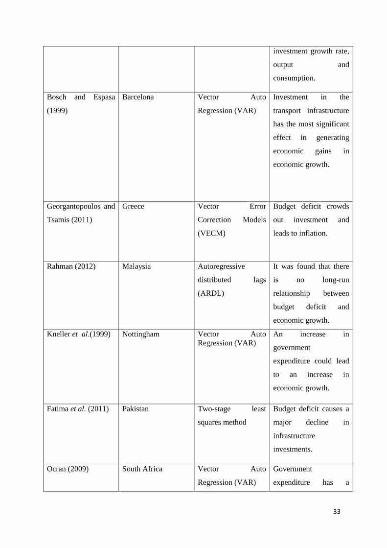
33

investment growth rate,

output and

consumption.

Bosch and Espasa

(1999)

Barcelona Vector Auto

Regression (VAR)

Investment in the

transport infrastructure

has the most significant

effect in generating

economic gains in

economic growth.

Georgantopoulos and

Tsamis (2011)

Greece Vector Error

Correction Models

(VECM)

Budget deficit crowds

out investment and

leads to inflation.

Rahman (2012) Malaysia Autoregressive

distributed lags

(ARDL)

It was found that there

is no long-run

relationship between

budget deficit and

economic growth.

Kneller et al.(1999)

Nottingham Vector Auto

Regression (VAR) An increase in

government

expenditure could lead

to an increase in

economic growth.

Fatima et al. (2011) Pakistan Two-stage least

squares method

Budget deficit causes a

major decline in

infrastructure

investments.

Ocran (2009) South Africa Vector Auto

Regression (VAR)

Government

expenditure has a

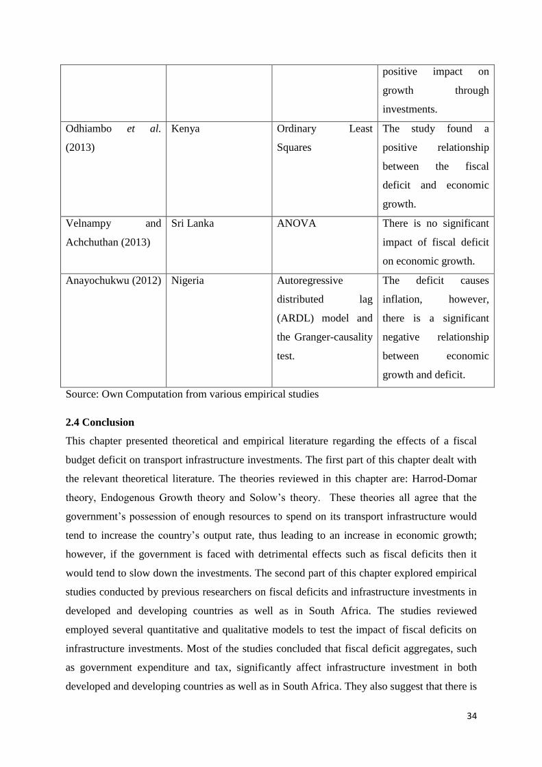
34

positive impact on

growth through

investments.

Odhiambo et al.

(2013)

Kenya Ordinary Least

Squares

The study found a

positive relationship

between the fiscal

deficit and economic

growth.

Velnampy and

Achchuthan (2013)

Sri Lanka ANOVA There is no significant

impact of fiscal deficit

on economic growth.

Anayochukwu (2012) Nigeria Autoregressive

distributed lag

(ARDL) model and

the Granger-causality

test.

The deficit causes

inflation, however,

there is a significant

negative relationship

between economic

growth and deficit.

Source: Own Computation from various empirical studies

2.4 Conclusion

This chapter presented theoretical and empirical literature regarding the effects of a fiscal

budget deficit on transport infrastructure investments. The first part of this chapter dealt with

the relevant theoretical literature. The theories reviewed in this chapter are: Harrod-Domar

theory, Endogenous Growth theory and Solow’s theory. These theories all agree that the

government’s possession of enough resources to spend on its transport infrastructure would

tend to increase the country’s output rate, thus leading to an increase in economic growth;

however, if the government is faced with detrimental effects such as fiscal deficits then it

would tend to slow down the investments. The second part of this chapter explored empirical

studies conducted by previous researchers on fiscal deficits and infrastructure investments in

developed and developing countries as well as in South Africa. The studies reviewed

employed several quantitative and qualitative models to test the impact of fiscal deficits on

infrastructure investments. Most of the studies concluded that fiscal deficit aggregates, such

as government expenditure and tax, significantly affect infrastructure investment in both

developed and developing countries as well as in South Africa. They also suggest that there is

35

a link between capital formation, which is investment in infrastructure, and economic growth.

However, it is important to note that in South Africa a large gap exists in literature regarding

the effects of fiscal deficits on infrastructure investments.

36

CHAPTER THREE

AN OVERVIEW OF THE SOUTH AFRICAN BUDGET DEFICIT AND

TRANSPORT INFRASTRUCTURE INVESTMENT

3. 1 Introduction

This chapter reviews developments and trends in the public transport infrastructure

investment for the period 1980-2011. The review highlights how changes in the budget

deficit contribute to the public transport infrastructure investment of the country for this

period. The chapter is divided into three sections: the first section provides the historical

background to the public transport infrastructure investment; the second section provides a

detailed analysis of the various variables used in the analysis, and the last section presents

concluding remarks.

3.2 Historical overview

South Africa is a developing country that has faced a number of transport challenges

including outdated rail rolling stock prone to malfunction, ports with high costs and less

optimal productivity rates as well as a road network that is under strain as 69% of freight is

being moved by road. The country also faced struggles with inadequate infrastructure

because of under-investment (National Treasury, 2012). This lack of investment, especially

evident in transport infrastructure such as railways, roads and ports has limited the rate at

which the local economy can grow without creating delays. Infrastructure development in

Africa has lagged behind the Western Hemisphere for centuries, even trailing Latin America

in recent decades. Infrastructure funding is largely provided by South Africa’s national

government and other companies have emerged in funding infrastructure; examples of these

are Eskom and Transnet.

In the interest of the long-term development of transport infrastructure in South Africa, it was

recommended that a Macro Transport Infrastructure Forum (MTIF), consisting of

representatives of all relevant parties, be established for South Africa. This would help to

achieve the political and economic objectives of the country. The MTIF would have the

responsibility of working with the government in order to determine a strategic focus

37

regarding transport infrastructure in South Africa and to pursue the development of a macro

plan by providing adjusted infrastructural development plans for the country.

The country has the ambition of having a multi-billion rand infrastructure development in

energy, electricity in particular, and transport infrastructure such as roads, railways and ports.

The government hopes that if it increases its investments further it will unlock the country’s

growth, which is what has been happening for the past seven years. With too much

expenditure on public transport infrastructure by the government it will make South Africa

reach a growth of 7% which will halve the high unemployment rate if the infrastructure plan

is successful (National Treasury, 2012).

3.2.1 South African Public Transport Infrastructure Investment

The International Transport Forum (2012) observed that Infrastructure investments are a key

determinant of performance in the transport sector. However, the sector lacks standardised

definitions and methods for measuring investment. The increasing mix of public and private

investors and operators in the transport sector adds to the complexity of measuring

investments and outcomes. Transport infrastructure has to be maintained and the

measurement of maintenance costs and outcomes differs widely across modes and countries.

However, the roadmap to achieving this aim has been less clear and is often challenging.

During the 1980s and 90s, investments in transport infrastructure were not taken into

consideration by the government, but were later recognized because of the explicit change

from non-market related controls towards market oriented policies (International Transport

Forum, 2012). The various role players were faced with the mounting challenge of using

transport systems to overcome the barriers of the apartheid spatial legacy, reconnecting

isolated nodes and communities long disconnected from opportunity.

Infrastructure has played a significant role in Africa’s recent economic turnaround, and will

need to play an even greater role if the continent’s development targets are to be reached. It is

a major constraint in doing business, and is found to depress firm productivity by around 40

percent. For most countries, the negative impact of deficient infrastructure is at least as large

as that associated with corruption, crime, financial market and red tape constraints (World

Bank, 2013).

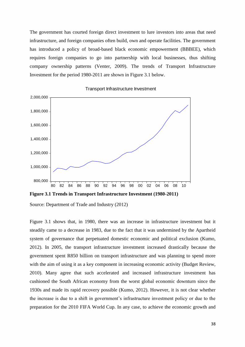
38

The government has courted foreign direct investment to lure investors into areas that need

infrastructure, and foreign companies often build, own and operate facilities. The government

has introduced a policy of broad-based black economic empowerment (BBBEE), which

requires foreign companies to go into partnership with local businesses, thus shifting

company ownership patterns (Venter, 2009). The trends of Transport Infrastructure

Investment for the period 1980-2011 are shown in Figure 3.1 below.

Figure 3.1 Trends in Transport Infrastructure Investment (1980-2011)

Source: Department of Trade and Industry (2012)

Figure 3.1 shows that, in 1980, there was an increase in infrastructure investment but it

steadily came to a decrease in 1983, due to the fact that it was undermined by the Apartheid

system of governance that perpetuated domestic economic and political exclusion (Kumo,

2012). In 2005, the transport infrastructure investment increased drastically because the

government spent R850 billion on transport infrastructure and was planning to spend more

with the aim of using it as a key component in increasing economic activity (Budget Review,

2010). Many agree that such accelerated and increased infrastructure investment has

cushioned the South African economy from the worst global economic downturn since the

1930s and made its rapid recovery possible (Kumo, 2012). However, it is not clear whether

the increase is due to a shift in government’s infrastructure investment policy or due to the

preparation for the 2010 FIFA World Cup. In any case, to achieve the economic growth and

800,000

1,000,000

1,200,000

1,400,000

1,600,000

1,800,000

2,000,000

80 82 84 86 88 90 92 94 96 98 00 02 04 06 08 10

Transport Infrastructure Investment

39

poverty alleviation goals set in its ASGISA agenda, the government had to ensure that

infrastructure investment would be accelerated and sustained in the long run.

Since 2006, there has been an increasing and upward trend of infrastructure investment in

South Africa. This increase was led by the power utility Eskom and transport group Transnet,

both of which were earmarked to receive 40% of the R372 billion the government set aside

for infrastructure development (National Treasury, 2012). Eskom was to spend R84 billion on

energy generation, transmission and distribution. Transnet was to spend R47 billion, R40

billion of which would be distributed to harbours, ports, railways and a petroleum pipeline.

Government spending on infrastructure in 2008 declined as a change in government and the

pressure to divert spending towards greater social expenditure mounted (Budget Review,

2010). In addition, government consumption expenditure ballooned – driven in large part by

the dramatic increase in the wage bill. This slant in expenditure towards current expenditure

and away from investment expenditure did not go unnoticed by ratings agencies. The lack of

investment caused a decrease or limit in the rate at which the economy can grow and one of

the highest increases in unemployment.

Despite government’s infrastructure drive, real growth in transport infrastructure investment

decreased in the recession year (2008-2009). However, prior to the recession, the government

realised the need for investment; hence, investments in the transport sector started to increase

in 2009 (Budget Review, 2010). South Africa has also seen large-scale infrastructural

investment in connection with the 2010 FIFA World Cup. In anticipation of millions of

soccer-loving tourists, the government spent over R40 billion to upgrade stadiums, airports,

trains and roads. Improvements in public transport, security, investment and tourism have

already been shown to benefit the people of our country. The hosting of the tournament also

resulted in job creation. South Africans demonstrated an explosion of national pride and

embraced each other, making the tournament a powerful nation-building tool.

3.3 Government Revenue 1980-2011

The South African tax revenue has been regarded as the largest source of budget revenue. If

the economy tends to be underperforming it will also perform poorly, hence, during the

economic downturn it showed a decreasing response. The Political Information and

Monitoring Services (PIMS) Budget Paper states that Revenue over-runs and a budget policy

favouring surpluses over the current medium-term expenditure period are related concepts.

http://www.eskom.co.za/

http://www.transnet.co.za/

40

Both embody aspects of a generally prudent and risk-averse approach taken by government to

macroeconomic management. These overruns have occurred under both the deficit and

surplus in previous years. Both revenue and expenditure convergence are firstly dependent on

the accuracy of the economic growth estimate. Revenue outcomes depend quite heavily on

growth outcomes since growth trends largely determine trends in the value of tax bases, such

as income and consumption. All else being equal, the more economic activity there is, the

more there is to be taxed, and the higher revenue collection will be for a given set of tax rates.

With the exception of 2003/04, actual tax revenues have considerably exceeded revenue

estimates. The value of revenue over-runs in the six years excluding 2003/04: R21.3 billion in

2004/05, R44.6 billion in 2005/06, R38.7 billion in 2006/07 and R14.5 billion in 2007/08

(National Treasury, 2012).

Total government revenue is budgeted to increase by a relatively substantial 11%y/y in fiscal

2013/2014, which seems high compared to a growth of only 6.1% in 2012/13; this is likely to

prove difficult to achieve given the modest GDP growth forecast (National Treasury, 2012).

The South African Revenue Service shows that it had another strong year in 2011 as it had

collected R742.7 billion in revenue which is more than the R4 billion the Finance Minister

Pravin Gordhan had budgeted for and R68 billion more than the amount collected in the

previous financial year. The government revenue is shown in Figure 3.2 below for the period

1980-2011.

Figure 3.2 Trends in Government Revenue (1980-2011)

Source: South African Reserve Bank (2012)

0

100,000

200,000

300,000

400,000

500,000

600,000

700,000

800,000

80 82 84 86 88 90 92 94 96 98 00 02 04 06 08 10

Government Revenue

41

From Figure 3.2, it is evident that tax on income and wealth over the period 1980 to 2011

grew at an exponential rate. The minimum tax revenue to ever be collected in the period was

in the year 1980 whilst the maximum was collected in 2008, decreased in 2009 and rose

again in 2011. Between 1994 and 2002, tax revenue rose at an increasing rate. This is because

the period was considered a period of fiscal and macroeconomic consolidation, were certain

tax policy changes and policy announcements that provide reference points for future reform

in the post 2002 tax reform era were made. Over this period, personal income tax was used to

raise the bulk of tax revenue; approximately 42.6 per cent was raised in 1999-2000 (National

Treasury, 2002). The period between 2002 and 2010 was a period of fiscal stabilisation. The

government was now able to comfortably adopt and support an expansionary fiscal stance as

set out in the 2002 budget, which is characterized by strong expenditure growth and

continued tax relief in the face of adverse global conditions. Since 2002, the National

Treasury stepped up the pace of fundamental income tax reforms with the distinct purpose of

aggressively broadening the tax base, thereby affording a significant rate reduction in line

with international trends (National Treasury, 2002). This broadening of the tax base increased

the tax revenue collected in current terms over the period leading up to 2011. Tax revenue, as

a percentage of GDP, has been significantly constant which shows that the government has

been more consistent in its tax collection over the years.

Revenue fell during the recession years thus creating the fiscal space for government to

expand investment, social grants and public-sector employment. Hence, the government

required higher levels of borrowing, resulting in a marked increase in debt-service costs

(Budget Review, 2010). The decline in revenue caused the government to increase or raise

its borrowing level and thus drove the country to a budget deficit. As the economy improved,

or recovered, from the recession the government revenue showed an increase in 2010 and

will continue to recover alongside the economic growth reducing the budget deficit.

3.4 Government Expenditure 1980-2011

Government spending, also called government expenditure is the amount of money that a

government spends on the public services provided to its citizens. Government expenditure

covers spending on goods and services like defence, and the judicial and education systems.

It excludes government transfers like social security and unemployment benefits (Trading

Economics, 2013). Expenditure varies with growth because lower growth may, amongst other

42

things, mean more eligible beneficiaries for entitlement-based spending. Over the past

decade, the redistributive and pro-poor character of public spending has significantly

improved, alleviating poverty and advancing social development. There is however growing

concern within government, in that additional budget allocations do not result in proper

improvements in service delivery. Government's ability to support accelerated growth,

increase employment, and reduce poverty and inequality is limited by two factors: the quality

of spending and the composition of spending, with a shift from consumption towards capital

investment becoming increasingly necessary (Trading Economics, 2013). The narrowing of

fiscal space, in combination with the erosion of the link between budget inputs and social

outputs, implies the need for additional measures to secure the country’s fiscal footing and

improve its quality of spending. While current levels of spending can be sustained over the

medium term, expenditure cannot grow at the rate at which it did over the last decade.

Every year the government spends several millions of rand on providing a better life for the

people living in South African. Over the years leading up to 2011, the South African government

strongly increased public spending (National Treasury, 2010). From 1980 to 1993 expenditure by

the apartheid government was to boost the economic, political and social wellbeing of South

Africans. During this period, government expenditure mainly benefited white South Africans who

selectively had access to good transportation systems, education, health facilities and recreational

services. Upon regime change in 1994, government expenditure focused on undoing the

inequalities created by the preceding apartheid regime. From 1994 to 2011, services that attracted

substantial attention from the ANC-led government were education, infrastructure (capital

expenditure), social welfare, debt, housing, health, protection, as well as water and agriculture

(National Treasury, 2010).

Government expenditure comes from the government’s revenue. This includes all

expenditure by the government towards infrastructural development in the country. The

rationale behind this is that improving the country’s infrastructure increases its long term

growth potential (Du Plessis and Smit, 2007). There seems to be advantages to a highly

functional infrastructure which include an increase in investment. Capital investment by the

public sector raises the country’s future growth potential by providing the economic

infrastructure required for trade and extended economic activity. This ultimately leads to

higher economic growth and trade.

43

Capital expenditure increased from R4 002 million in 1980 to R10 685 million in 1993,

averaging R8 203 million per year over thirteen years (DTI, 2011). During this period low

government revenue collections restricted the government’s capital investment. Logically, it

is also imperative to note that the government’s developmental obligation was only focussed

on a few communities that furthered the interests of minority white community. Black South

African communities were totally neglected and disenfranchised which resulted in less

government obligation to spend on investment (Levy, 1999). Nevertheless, upon attaining

democracy in 1994, government capital expenditure grew sharply as a reflection of an

inclusive budget that did not discriminate, on any account, in terms of race or gender.

Specific attention was, however, given to the previously disadvantaged black South Africans

(National Treasury, 2007). Government investment expenditure exponentially increased from

a minimum of R11 358 million in 1994 to R80 819 million in 2011, averaging R38 382

million per year over the years (DTI, 2011). The great public investment expenditure was a

result of social infrastructure programmes such as hospital revitalisation, school building and

sanitation, as well as others (National Treasury, 2010). These activities are crucial in the

delivery of government services and have thus received significant attention. The National

Treasury (2010) also postulated that spending on capital averaged 5.8 per cent of total

expenditure between 1994 and 2011 and is expected to average 7.2 per cent between 2011

and 2013. For the period 1980 to 2011, government expenditure exponentially increased from

R4 002 million (in 1980) to R80 819 million (in 2011), averaging R 24 753 million per year

over this period. The highest capital expenditure recorded over the period is R89 437 million,

which was observed in 2008 (DTI, 2011). According to the National Treasury (2010), the

figure was a result of massive government spending towards a successful 2010 FIFA Soccer

World Cup. Government expenditure over the period 1980 to 2011 is shown by Figure 3.3.

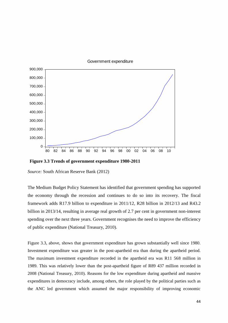
44

Figure 3.3 Trends of government expenditure 1980-2011


The Medium Budget Policy Statement has identified that government spending has supported

the economy through the recession and continues to do so into its recovery. The fiscal

framework adds R17.9 billion to expenditure in 2011/12, R28 billion in 2012/13 and R43.2

billion in 2013/14, resulting in average real growth of 2.7 per cent in government non-interest

spending over the next three years. Government recognises the need to improve the efficiency

of public expenditure (National Treasury, 2010).

Figure 3.3, above, shows that government expenditure has grown substantially well since 1980.

Investment expenditure was greater in the post-apartheid era than during the apartheid period.

The maximum investment expenditure recorded in the apartheid era was R11 568 million in

1989. This was relatively lower than the post-apartheid figure of R89 437 million recorded in

2008 (National Treasury, 2010). Reasons for the low expenditure during apartheid and massive

expenditures in democracy include, among others, the role played by the political parties such as

the ANC led government which assumed the major responsibility of improving economic

0

100,000

200,000

300,000

400,000

500,000

600,000

700,000

800,000

900,000

80 82 84 86 88 90 92 94 96 98 00 02 04 06 08 10

Government expenditure

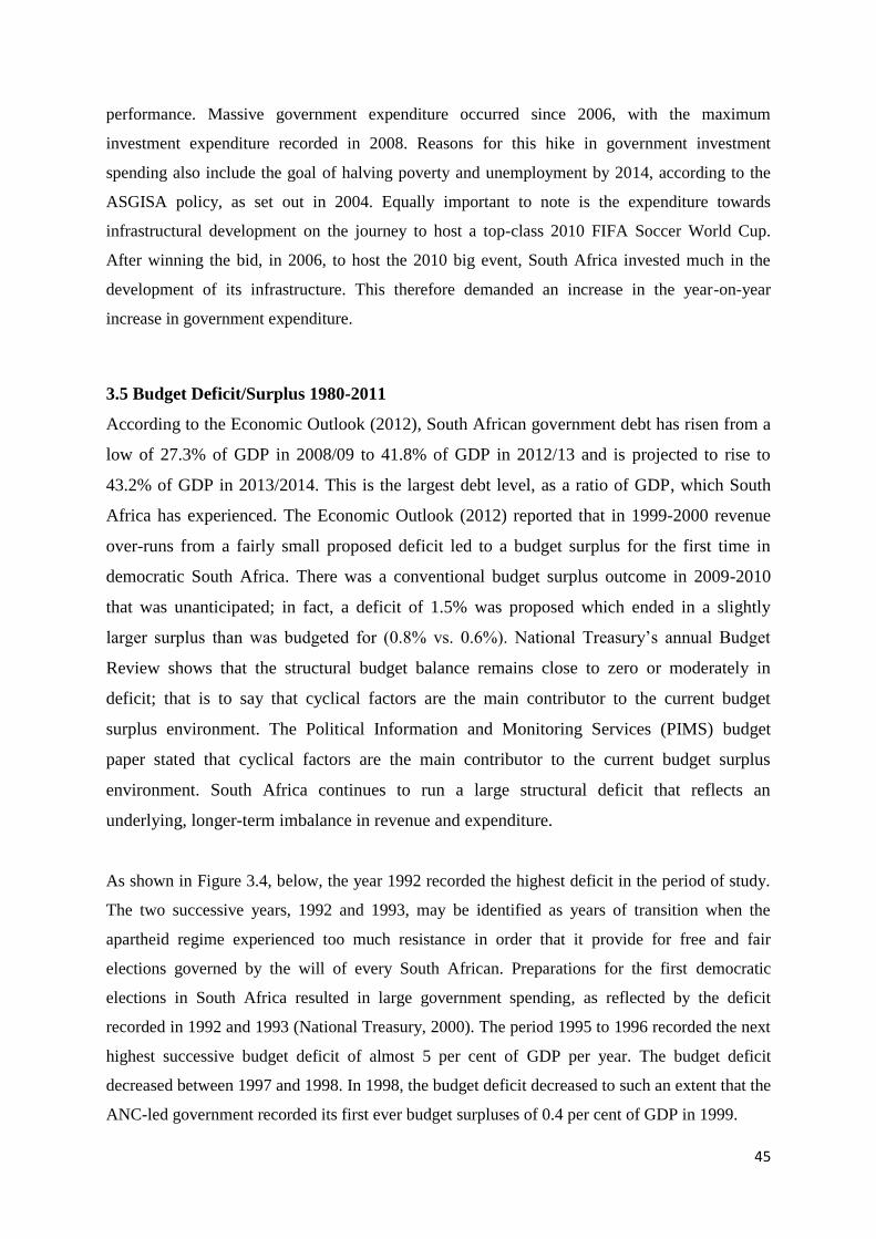
45

performance. Massive government expenditure occurred since 2006, with the maximum

investment expenditure recorded in 2008. Reasons for this hike in government investment

spending also include the goal of halving poverty and unemployment by 2014, according to the

ASGISA policy, as set out in 2004. Equally important to note is the expenditure towards

infrastructural development on the journey to host a top-class 2010 FIFA Soccer World Cup.

After winning the bid, in 2006, to host the 2010 big event, South Africa invested much in the

development of its infrastructure. This therefore demanded an increase in the year-on-year

increase in government expenditure.

3.5 Budget Deficit/Surplus 1980-2011

According to the Economic Outlook (2012), South African government debt has risen from a

low of 27.3% of GDP in 2008/09 to 41.8% of GDP in 2012/13 and is projected to rise to

43.2% of GDP in 2013/2014. This is the largest debt level, as a ratio of GDP, which South

Africa has experienced. The Economic Outlook (2012) reported that in 1999-2000 revenue

over-runs from a fairly small proposed deficit led to a budget surplus for the first time in

democratic South Africa. There was a conventional budget surplus outcome in 2009-2010

that was unanticipated; in fact, a deficit of 1.5% was proposed which ended in a slightly

larger surplus than was budgeted for (0.8% vs. 0.6%). National Treasury’s annual Budget

Review shows that the structural budget balance remains close to zero or moderately in

deficit; that is to say that cyclical factors are the main contributor to the current budget

surplus environment. The Political Information and Monitoring Services (PIMS) budget

paper stated that cyclical factors are the main contributor to the current budget surplus

environment. South Africa continues to run a large structural deficit that reflects an

underlying, longer-term imbalance in revenue and expenditure.

As shown in Figure 3.4, below, the year 1992 recorded the highest deficit in the period of study.

The two successive years, 1992 and 1993, may be identified as years of transition when the

apartheid regime experienced too much resistance in order that it provide for free and fair

elections governed by the will of every South African. Preparations for the first democratic

elections in South Africa resulted in large government spending, as reflected by the deficit

recorded in 1992 and 1993 (National Treasury, 2000). The period 1995 to 1996 recorded the next

highest successive budget deficit of almost 5 per cent of GDP per year. The budget deficit

decreased between 1997 and 1998. In 1998, the budget deficit decreased to such an extent that the

ANC-led government recorded its first ever budget surpluses of 0.4 per cent of GDP in 1999.

46

According to the National Treasury (2000), reasons for the shrinking deficits include the

government’s desire to achieve a marked redistribution of spending in favour of previously

disadvantaged communities using a sound fiscal policy framework that eliminates unsustainable

deficit spending and increasing public debt, among other issues. This was initiated to support the

sustainability of government finances and contribute to ensuring that the economic achievements

of the past years are protected from cyclical and external risks (National Treasury, 2008). The

deficit in 2009, among other reasons, emanates from the government intensifying its fixed capital

investment towards the 2010 FIFA World Cup. The Budget Deficit/Surplus from the period

1980-2011 is shown in Figure 3.4 below.

Figure 3.4 Trends in the Budget deficit/Surplus (1980-2011)


The period beginning in the early 1980s and ending with the transition to a new constitutional

and political environment was therefore marked by increasing government expenditure and

taxation, with the fiscal deficit increasing to 6.8 per cent of GDP in 1992. If moderate deficits

are run to facilitate infrastructure expansion that promises future economic returns, the deficit

may be seen in a positive light as an enabling fiscal action. The budget deficit declined to 3.0

per cent of GDP; public debt relative to GDP declined from 49.7 per cent in 1994 to 44.4 per

cent in 1998 and average borrowing costs decreased sharply, thus providing room for

-8

-4

0

4

8

12

80 82 84 86 88 90 92 94 96 98 00 02 04 06 08 10

Deficit/Surplus

47

government to spend more on social services and infrastructure (Naraidoo and Schoeman,

2011).

Although government had achieved a substantial reduction in its budget deficit target, from

6.8 per cent of GDP in 1993 to 0.6 per cent in 2008, the scenario has, in the interim, changed

again (Budget Review, 2010). This is mainly due to the slowdown in the world economy,

which also affected the revenue base of the South African economy. However, the policy of

fiscal prudence, during the period 2003 to 2008, resulted in a substantial decline in real debt

service cost, while the real growth rate of the economy increased considerably. Nevertheless,

there still exists a gap between the real debt service cost and the real growth rate since the

former exceeds the latter. Furthermore, it appears that public debt and budget deficit

reductions have been achieved at the expense of a relative reduction in service delivery

expenditure, as is evident in the reduction in the ratio of education expenditure to GDP from

an average of 6.21 per cent during the period 1990 to 1999, to an average of 5.6 per cent

during the period 2000 to 2008; and a reduction in health expenditure relative to GDP to an

average of 2.84 percent between 2000 to 2008 from 1990 to 1999 average of 2.93 per cent

(Naraidoo and Schoeman, 2011). During the economic downturn in 2008-2009 the revenue

fell; this required a significant increase in borrowing that resulted in an increase in the budget

deficit. The 2010 Medium Term Budget Statement Policy reflected that the budget deficit is

projected to narrow from 5.3 per cent of GDP to 3.2 per cent by 2013/14, reflecting a strong

recovery in revenue and moderate growth in spending.

Fiscal management will be more challenging towards the end of the forecast period because

deeper consolidation will be needed to stem the rise in debt service costs and protect investor

confidence. The government will therefore need to make some tough choices in the face of

persistent pressure to spend more on infrastructure, social welfare and wages especially in the

run-up to the 2014 elections (National Treasury, 2012).

3.6 Foreign Direct Investment 1980-2011

FDI (Foreign Direct Investment) is defined as private capital flows into a country different to

that in which the parent firm is situated. Foreign Direct Investment has become increasingly

important in a developing country in order to attract substantial and rising amounts of inward

FDI (Khaliq and Noy, 2007). Foreign Direct Investment (FDI) is seen as an increasingly

important driver of economic growth and development, particularly within the developing

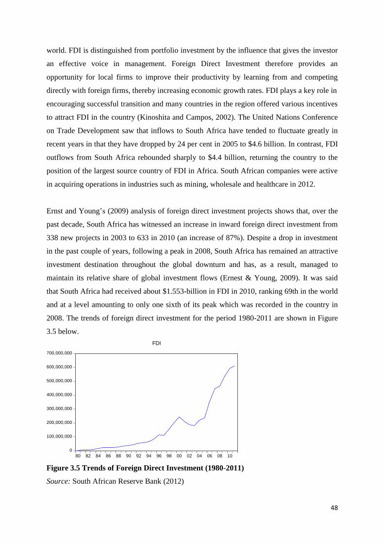
48

world. FDI is distinguished from portfolio investment by the influence that gives the investor

an effective voice in management. Foreign Direct Investment therefore provides an

opportunity for local firms to improve their productivity by learning from and competing

directly with foreign firms, thereby increasing economic growth rates. FDI plays a key role in

encouraging successful transition and many countries in the region offered various incentives

to attract FDI in the country (Kinoshita and Campos, 2002). The United Nations Conference

on Trade Development saw that inflows to South Africa have tended to fluctuate greatly in

recent years in that they have dropped by 24 per cent in 2005 to $4.6 billion. In contrast, FDI

outflows from South Africa rebounded sharply to $4.4 billion, returning the country to the

position of the largest source country of FDI in Africa. South African companies were active

in acquiring operations in industries such as mining, wholesale and healthcare in 2012.

Ernst and Young’s (2009) analysis of foreign direct investment projects shows that, over the

past decade, South Africa has witnessed an increase in inward foreign direct investment from

338 new projects in 2003 to 633 in 2010 (an increase of 87%). Despite a drop in investment

in the past couple of years, following a peak in 2008, South Africa has remained an attractive

investment destination throughout the global downturn and has, as a result, managed to

maintain its relative share of global investment flows (Ernest & Young, 2009). It was said

that South Africa had received about $1.553-billion in FDI in 2010, ranking 69th in the world

and at a level amounting to only one sixth of its peak which was recorded in the country in

2008. The trends of foreign direct investment for the period 1980-2011 are shown in Figure

3.5 below.

Figure 3.5 Trends of Foreign Direct Investment (1980-2011)


0

100,000,000

200,000,000

300,000,000

400,000,000

500,000,000

600,000,000

700,000,000

80 82 84 86 88 90 92 94 96 98 00 02 04 06 08 10

FDI

49

As a result, African countries in the 1980s reached a level where domestic firms were

allowed to be free of small markets and low productivity. This helped to build stronger links

between investment and exporting allowing free trade and free entry into foreign markets.

In this context, the shift in composition of FDI flows towards manufacturing was also slower

than elsewhere and was usually the result of heavy protection providing a captured market,

with insufficient attention to export promotion. This deterioration damaged investment

prospects and increased the sector’s vulnerability to further shocks, but was even more

decisive in constraining investment in the primary sector, where much production was

organized through state-owned companies in urgent need of restructuring and recapitalization

(UNCTAD, 2005). The developing countries have increasingly grown to receive the flow of

foreign direct investment that create an important infrastructure, but will they have an ability

to manage and respond to international economic fluctuations (Rena and Kefela, 2011).

3.7 Real Gross Domestic Product 1980-2011

South Africa’s economic development has been dominated by colonialism and apartheid.

Economic growth was conditioned, on the one hand, by changes in commodity prices and, on

the other, by a low-productivity and low-employment approach to production that took

advantage of limited competition from imports and cheap intermediate inputs. Public

transport, roads, and housing were insufficient to absorb migrants from rural or far-flung

industrial areas. Formal sector wage bargaining reflected the complex nature of households

split between rural and urban areas, elevated dependency ratios, and the high costs of

inefficient transport systems (UNCTAD, 2004b). Monetary policy became accommodative

by the 1980s, thus resulting in consistent negative real interest rates. These policies were

made possible by rigorous exchange controls, which prevented capital from crossing the

border. In the same period, public spending rose strongly in an effort to extend social

infrastructure and increase subsidies to industry. This resulted in large budget deficits and

rising debt levels.

The South African government recognised the importance of transport, transport

infrastructure in particular, and so it launched policy strategies such as the Reconstruction

and Development Programme (RDP 1994), the Growth Employment and Redistribution

(GEAR 1996) programme and the Accelerated Shared Growth Initiative for South Africa

(Mlambo-Ngcuka, 2006). The GEAR policy strategies focused primarily on improving output

50

and employment, increasing infrastructure allocations and encouraging trade. The strategy

achieved redistribution and improvement in basic living conditions because it generated some

increases in economic growth, low inflation, high demand, high commodity prices and rising

consumption. However, it was not a success in meeting the specified the employment

projections.

The Accelerated Shared Growth Initiative for South Africa (ASGISA) was developed when

the government saw the need for greater investments in infrastructure and other areas

contributing to economic growth and ensuring that the poor and unemployed share in the

country’s economic growth (Mlambo-Ngcuka, 2006). With the ASGISA strategy being

present, the government decided to make special budget allocations towards infrastructure

development in order to achieve the targeted 6% economic growth rate. ASGISA aimed to

develop scarce skills in the country by providing effective solutions such as special training

programmes for those who were inexperienced. The policy strategy failed to do what it had

aimed for and what the government had expected out of it.

There has been a considerable improvement in economic growth which averaged at about 3

per cent during the first decade of freedom. Since 2004, growth has tended to exceed 4 per

cent per year, reaching about 5 per cent in 2005 (National Treasury, 2006). According to Du

Plessis et al. (2007), if economic growth is increased, unemployment levels will fall. The

World Bank (2009) indicated that a 2 per cent increase in growth rates will result in a

reduction in unemployment ranging from 1 to 7 per cent, depending on the country.

South Africa's economy has been completely overhauled since the advent of democracy in

1994. The GDP growth rate analyses the economic performance of South Africa. The

economy rose at a real rate of 1.2% from 1994 to 2000, according to the statistics of the

South African Reserve Bank (South African Reserve Bank, 2012). Economic growth

eventually rose in 1996, because of the executed policies (GEAR) of the government of that

period and the economy showed a steady increase in economic growth to the level of 4% in

this year. This policy intended to accelerate growth that would be associated with the right

technology, was envisaged to increase employment while enabling the labour intensive

investment to rise. This was also intended to result in a major boost in the economy, and new

jobs were to be created each. This major increase in employment meant that the economy

51

would operate at full employment, thus fully utilising all its resources. The trends in real

gross domestic product, from the year 1980 to 2011, are shown in Figure 3.6.

Figure 3.6 Trends in RGDP (1980-2011)


After 1996, economic growth eventually declined in 1997 until an extreme decline was

evident in 1998, by 2.1%, which was caused by the accumulation of joblessness, an

accelerated rate of inflation due to the expansion of money supply, the collapse of the prices

of commodities, and a decline in foreign investment which also resulted in lower interest

rates. The economy’s growth rate declined to 0.5% (Loots, 1998). The economic growth rate

increased again after 1998 due to the tightening of monetary policy; this means that money

supply was decreased which resulted in a fall in inflation and increase in interest rates. Real

growth in GDP, over the past 10 years, has been strong, consistently above 2.5% per annum,

and reaching 5.5% in 2007.

South Africa was in a recession from 2008 to 2009; there were therefore only a few

investments made in the country because investors were reluctant to invest in a country where

there would be no returns or lower returns on their investment. This caused the economic

growth to decline since it had a negative effect on people, especially the poor (Catshile,

2010).

13.7

13.8

13.9

14.0

14.1

14.2

14.3

14.4

14.5

80 82 84 86 88 90 92 94 96 98 00 02 04 06 08 10

LOG_RGDP

52

The recession that was in place in 2008 and 2009 did not last long. The government

intervened and the country was subsequently attained its full capacity (Catshile, 2010). This

happened because it was preparing to host the 2010 FIFA World Cup so it quickly recovered

from the financial crisis and operated at full employment; there were now increased

investments taking place and consumers were no longer vulnerable to the high costs of goods

and services, while inflation was at a normal rate where the interest rates were low.

Real GDP is forecast to grow by 3.7% in 2011, as a result of higher consumer spending,

increased business investment and stronger external demand. Although growth will be too

slow to make an impact on unemployment, higher wages for those who work will support

consumer demand, as will low interest rates and subdued inflation (Ernst and Young, 2012).

Business, which has been cautious about investing in the wake of the recession, will regain

confidence in line with the wider upswing and increase the pace of investment in new

capacity. The government will also remain supportive of growth via an ongoing fiscal

stimulus, directed towards investment in infrastructure in particular.

3.8 Conclusion

This chapter provided an overview of the fiscal deficit and transport infrastructure investment

trends in South Africa, over the period 1980 to 2011. It was discovered that government tax

revenue grew exponentially between 1980 and 2011. With the country obtaining democracy

in 1994, government revenue suddenly increased in South Africa. The country experienced

increased investment, lifting of consents levelled against the apartheid regime, productivity

due to technological advancements and mobility, among other things. Government

investment increased significantly since 1980. The rationale behind the massive expenditures

in a democratic South Africa include, among others, the responsibility assumed by the ANC-

led government to create sustainable and inclusive economic development. The last part of

this chapter highlighted the policy tools implemented by the government to achieve

macroeconomic equilibrium. Several policy tools used by the government since 1994 include:

the Reconstruction and Development Programme (RDP), the Growth, Employment and

Redistribution Policy (GEAR), the Accelerated and Shared Growth Initiative for South Africa

(ASGISA) and the New Growth Path (NGP). These policy tools have helped to redistribute

wealth across races and improve the transport infrastructure in South Africa.

53

CHAPTER FOUR

RESEARCH METHODOLOGY

4.1 Introduction

This chapter presents the methodology employed in the investigation of the impact of the

budget deficit on transport infrastructure investment in South Africa. The empirical model for

the study and the relevant data issues are presented herein. The first part of the chapter

specifies the model and how estimation of the model was applied. This is followed by

specifying the data that was used, the definition of variables and outlining the expected

results. The last part of the chapter explores various tests for the model, including

stationarity, cointegration error correction and diagnostic testing.

4.2 Model specification

To determine the relationship between government budget deficit and transport infrastructure

investment in South Africa, this study uses the model specified by Hadiwibowo (2010) in his

analysis of the effects of fiscal policy on investment and economic growth in Indonesia. The

study applies the explanatory variables such as the budget deficit made up of government

expenditure and government revenue as well as foreign direct investment. Therefore, the

modified version of the model is formulated as follows:

TIIt t t ……………….………….. 4.1

Where: , β1, β2 and β3 are the coefficients and ε is the error term.

TII = Transport Infrastructure Investment

(T-G) = Budget Balance

GDP = Gross Domestic Product

FDI = Foreign Direct Investment

D = Dummy Variable

ε = error term

t = Time

54

4.3 Definition of the variables and data sources

Transport Infrastructure Investment is the gross capital formation made by the government in

the transport sector. Quarterly time series data for transport infrastructure investment, from

the first quarter of 1990 to the fourth quarter of 2009, was used in the estimation and was

sourced from the Department of Trade and Industry’s (DTI) economic database.

Gross Domestic Product (GDP) is the market value of all final goods and services produced

within the country over a given period of time. Quarterly time series data for GDP (constant

market prices) from the first quarter of 1990 to the fourth quarter of 2009 was used in the

estimation and was sourced from the South African Reserve Bank.

Budget Balance is government revenue minus the government expenditure of a country.

Quarterly time series data for budget balance from the first quarter of 1990 to the fourth

quarter of 2009 was used in the estimation and was sourced from the South African Reserve

Bank.

Foreign Direct Investment is the inflow of foreign capital into the country’s borders.

Quarterly time series data for foreign direct investment from the first quarter of 1990 to the

fourth quarter of 2009 was used in the estimation and was sourced from the South African

Reserve Bank.

4.4 Expected Priori

In estimating a regression equation, all economic variables are expected to conform to

economic theory. This research follows on literature reviewed in Chapter 2 and estimates a

relationship that conforms to economic theory. The coefficient β2 is expected to have a

positive relationship with transport infrastructure investment. When GDP increases it tends to

increase the government expenditure and leads to an increase in transport infrastructure

investment.

The coefficient β3 is expected to be positively related to transport infrastructure investment

because foreign investment supports growth in developing countries by increasing

government spending which covers public investments.

The coefficient β4 is a dummy variable taking 1 if deficit and 0 otherwise. An increase in the

deficit is expected to have a negative relationship with transport infrastructure investment.

55

4.5 Estimation Techniques

There are several techniques available for parameter estimation, ranging from classical

regression methods to cointegration based techniques. The former is based on the assumption

that all the variables included in a regression are stationary. However, most time series data is

not stationary in their levels such that estimations based on this technique will be

meaningless. Differencing the variables to mechanically turn them stationary has been a

preferred approach to dealing with this problem as it can offer very useful long run

information that may be in the data. The techniques employed to test for stationarity and co-

integration are reviewed in this section.

4.5.1 Testing for Stationarity/Unit Root

A stationary series is defined as one with a constant mean, constant variance and constant

auto covariance with each lag given (Brooks, 2003:319). A series that is not stationary is

referred to as non stationary. In addition, a series is said to be integrated and is denoted as I

(d), where d is the order of integration. The order of integration refers to the number of unit

roots in the series, or the number of differencing operations it takes to make a variable

stationary.

In the classical regression model, the focus is on the relationship between stationary

variables, but most of the variables usually follow a non stationary path. Variables that have a

linear relationship (non-stationary) can produce misleading results as they might show trends.

Stationarity refers to testing and making sure that the series are integrated of the same order.

Gujarati (2003: 806) shows that if the dependent variable is a function of a non stationary

process, the regression will produce meaningless results. In other words, the dependent

variable will follow the trend of its explanatory variables. In such a case, the results will be

spurious. In fact, the t-ratio on the slope of the coefficient would be expected not to be

significantly different from zero and the value for R2

would be very low even though the

trending variables are completely unrelated. Thus, the t-ratio will not follow the t-distribution

and the f-ratio will not follow the f-distribution. Consequently, unit root or stationarity tests

should be done on all the variables before proceeding with the tests for the cointegration and

estimation of parameters. In this study, the Augmented Dickey-Fuller and Phillips Perron unit

root tests are discussed.

56

4.5.2 The Augmented Dickey–Fuller test and Phillips Perron

The Augmented Dickey-Fuller and Phillips Perron are unit root tests for stationarity.

Variables are tested for stationarity because most economic series are not stationary in their

levels, which lead to estimations being meaningless. The ADF supplements the test by using

lags to the dependent variable. The alternative model in the ADF case can be written as:

∆yt = γ yt-1∑ ∆yt-1+1 +µt.................................................................................................. 4.2

In equation (4.2) yt is the relevant time series, ∆ is a first difference operator, t is a linear

trend and ut is the error term. The error term should satisfy the assumptions of normality,

constant error variance and independent error terms. The lags of ∆yt now infuse any dynamic

structure present in the dependent variable, to ensure that ut is not auto correlated. Equations

(4.2) represent the estimated without including a trend term and without a constant.

The equation with a constant and no trend is represented

∆yt= a0 + γ yt-1 + ∑ ∆yt-1+1 +µt........................................................................................4.3

The equation with both a trend and a constant is given by:

∆yt = a0 + γ yt-1 a2 ∑ ∆yt-1+1 +µt..................................................................................... 4.4

In these models:

= γ - (1- ∑ )

and

β = - ∑

The ADF test corrects for high-order serial correlation by adding a lagged differenced term

on the right-hand side of the equations. If the calculated statistic is less (in absolute terms)

than the MacKinnon (1991, 1996) values, which are used by the E-views 7 software, the null

hypothesis is accepted and will therefore mean that there is a unit root in the series. In other

words, it means the time series is not stationary. The opposite is true when the calculated

statistic is greater than the MacKinnon critical values. However, in this ADF equation the

coefficient of interest is γ, if γ = 0, the equation is entirely in first difference form and so has

no unit root. If the coefficients of a difference equation sum up to 1, at least one characteristic

root has unity. On the equations, if ∑ai =1, γ =0 and the system has a unit root.

57

4.5.3 Cointegration and vector error correlation modelling (VECM)

The reason for undertaking cointegration tests is to determine whether all the variables in the

unemployment model are cointegrated. According to Gujarati (2003:830), cointegration of

two or more times series suggest that there is a long-run or equilibrium relationship between

them. Cointegration exists when two or more series are linked to from an equilibrium

relationship spanning in the long run. Variables are defined as co-integrated if a linear

combination of them is stationary. A cointegrating relationship may, in other words, be seen

as a long-term or equilibrium occurrence. This is because it is possible that co-integrating

variables may deviate from their relationship in the short run, but their association would

return in the long-run. There are different ways of testing cointegration, such as: the Engle

Granger approach which is residual based and the Johansen and Julius technique which is

based on maximum likelihood estimation on a VAR system. However, the majority of these

techniques have numerous problems when applied to multivariate models. The Johansen

technique will be used in this study because it has emerged as a powerful and popular

technique in determining cointegration. The purpose of this cointegration test is to determine

whether the variables in the growth model are cointegrated or not. The Johansen (1991, 1995)

technique has become an essential tool in the estimation of models that involve time series

data. This approach is preferred as it captures the underlying time series properties of the

data and is a systems equation test that provides estimates of all cointegrating relationships

that may exist within a vector of non stationary variables or a mixture of stationary and non

stationary variables (Harris, 1995: 80). The Johansen technique has several advantages over

other cointegration based techniques. This technique is preferred in this study as it will allows

estimating a dynamic error correction specification, which provides estimates of both the

short and the long run dynamics in the growth model.

The following steps are involved when implementing the Johansen technique:

Step 1: Testing the order of integration

The first step in the Johansen approach is to test for the order of integration of the

variables under examination. All variables are preset to assess their order of

integration. When all the variables are integrated of the same order we can then

proceed with the co-integration test. The data must be plotted to see if a linear

time trend is present.

Step 2: Setting the appropriate lag length of the model

58

Estimate the model and determine the rank of П.

Step 3: Choosing the appropriate model regarding the deterministic components in the

multivariate system

Analyse the normalised cointegrating vector(s) and speed of adjustment coefficients.

Step 4: Determine the number of co-integrating vectors

Apply causality tests on the error correction model to identify a structural model and

determine whether the estimated model is reasonable.

Assume a vector: Xt = [LTII, LFDI, RGDP, DUMMY] and assume the vector is in VAR

representation of the form:

Xt = z + ∑ Xt-1 + µt....................................................................................................... 4.5

where z is a (n x 1) vector of deterministic variables, ε is a (n x 1) vector of white noise error

terms and ∏ is a (n x n) matrix of coefficients. In order to use the Johansen test, the VAR

(4.5), above, needs to be turned into a VECM; specification (Brooks, 2002: 403), which may

be specified as:

∆Xt= z + ∑ Xt-1 +µt....................................................................................................... 4.6

Where Xt is a vector of I (1) variables defined above, Δ Xt are all I (0) variables, Δ indicates

the first difference operator, B is a (n x n) coefficient matrix and ∏is a (n x n) matrix whose

rank determines the number of cointegrating relationships. The Johansen’s cointegration test

is to estimate the rank of the∏ matrix (r) from an unrestricted VAR and to test whether to

reject the restrictions implied by the reduced rank of ∏. If ∏is of full rank (r = n), it suggests

that variables are level stationary and if it is of zero rank (r = 0), no cointegration exists

among the variables. Alternatively, if ∏is of reduced rank (r<n), then there exists (n x r)

matrices α and β such that:

αβ`................................................................................................................................... 4.7

where α represents the speed of adjustment matrix, indicating the speed with which the

system responds to last period’s deviations from the equilibrium relationship and β is a

matrix of long run coefficients (Brooks, 2002: 404).

Before an attempt to rank the cointegrating relationship is made there are two steps that need

to be followed. The Johansen test requires an optimal lag length (k) to be selected and the

choice of the deterministic assumption. The rationale behind the selection of the lag length is

59

because the Johansen test can be affected by the lag length of the Vector Error Correction

Model (VECM). A set of information criteria is used in the selection of the optimal lag

length, this includes: the sequential modified likelihood ratio (LR), Akaike information

criterion (AIC), Final prediction error (FPE) Schwarz, information criterion (SC) and the

Hannan-Quinn information criterion (HQ). This information criteria usually centers around

one lag length but if its components are inconsistent then the AIC and SC are considered to

be the best predictors because of the prediction power.

The second step is the choice of the deterministic assumption that the Johansen test requires

in testing for cointegration. Various types of VAR can be estimated based on five

deterministic trend assumptions, for example, with or without a constant and trend in

cointegrating term and with or without a constant in the VAR equations. E-views 7

specifically provides the following deterministic trend assumptions that there is no

deterministic trend in the data and no intercept or trend in the VAR and in the cointegrating

equation (CE); there is no deterministic trend in the data, but an intercept in the CE and no

intercept in VAR; there is a linear deterministic trend in the data and an intercept in CE and

test VAR; there is a linear deterministic trend in data, intercept and trend in CE and no trend

in VAR; for a quadratic deterministic trend in data, intercept and trend in CE and linear trend

in VAR.

After the correct VAR order (k) and the deterministic trend assumption has been selected, the

rank of the ∏matrix can then be tested. The Johansen and Juselius (1990) has two variants of

the reduced rank test for determining the cointegration space, namely, the maximum

eigenvalue (λ-max) and the trace statistics (λ-trace). In interpreting the results of the null

hypothesis of no cointegrating vector can be rejected, it indicates that there is a long run

relationship among the variables in the model.

The Johansen and Juselius tests are represented by the following equations:

λ-max (r, r + 1) = -T ∑ (1- λi)……………………………………………..…..…......4.8

λ-trace (r) = -T∑ (1- λi) ................................................................................................4.9

Where: r is the number of cointegrating vectors, λi is the estimated values of the

characteristics root (also called eigenvalues) and T is the number of usable observations. The

larger λi, is, the more large and negative will be the test statistic. Therefore, if the eigenvalue

60

is non-zero, then ln (1λi) <0∀i>1., The largest for eigenvalue to have a rank of 1, it should be

significantly non-zero, while other eigenvalues will not be significantly different from zero.

The trace statistic sequentially tests the null hypothesis that the number of cointegrating

relations is r against the alternative of k cointegrating relations, where k is the number of

endogenous variables. The maximum eigenvalue conducts separate tests on each eigenvalue

and has as its null hypothesis that there are r cointegrating vectors against an alternative of

r+1 (Brooks, 2003: 405). Both these tests compare the eigenvalue and trace statistic values to

critical values. For both tests, if the test statistic is greater than the critical values, the null

hypothesis that there are r cointegrating vectors is rejected in favour of the corresponding

alternative hypothesis.

However, the trace and maximum eigenvalue statistics may yield contradictory results. To

deal with this problem, Johansen and Juselius (1990) recommend the examination of the

estimated cointegrating vector and basing one’s choice on the interpretability of the

cointegrating relations. Alternatively, Luintel and Khan (1999: 392) show that the trace test is

more robust than the maximum eigenvalue statistic in testing for cointegration. The two

approaches will be considered in this study when faced with such a problem.

After all the cointegrating vectors have been identified a Vector Error Correction Model may

be estimated. A VECM is merely a restricted VAR designed for use with non stationary

series that have been found to be cointegrated. The specified cointegrating relation in the

VECM restricts the long run behavior of the endogenous variables to converge on their

cointegrating relationships, while allowing for short run adjustment dynamics. Once

estimation is complete, the residuals from the VECM must be checked for diagnostic tests

such as normality, heteroskedasticity and autocorrelation, which are discussed in the next

sub-section

4.5.4 Diagnostic Tests

This is an important stage in the impact of a budget deficit on transport infrastructure

investment because it validates the parameter estimation outcomes achieved by the estimated

model. Diagnostic checks test the stochastic properties of the model such as residual

autocorrelation, heteroskedasticity and normality, among others. The multivariate extensions

of these residuals tests will be applied in this study; hence, they are briefly discussed herein.

61

4.5.4.1 Autocorrelation LM Test

The Lagrange Multiplier (LM) test used in this study is a multivariate test statistic for

residual serial correlation up to the specified lag order. Harris (1995: 82) argues that the lag

order for this test should be the same as that of the corresponding VAR. The test statistic for

the chosen lag order (m) is computed by running an auxiliary regression of the residuals (tμ)

on the original right-hand explanatory variables and the lagged residuals (m t− μ). Johansen

(1995) presents the formula of the LM statistic and provides details on this test. The LM

statistic tests the null hypothesis of no serial correlation against an alternative of auto

correlated residuals.

4.5.4.2 Heteroscedasticity test

According to Brooks (2003:148), there are a number of formal statistical tests for

heteroscedasticity. One such popular test is White’s (1980) general test for heteroscedasticity.

The test is useful because it has a number of assumptions; for example, it assumes that the

regression model estimated is of the standard linear. After running the regression residuals

are obtained and then test regression is run by regressing each product of the residuals on the

cross products of the regressors and testing the joint significance of the regression. The null

hypothesis for the White test is homoskedasticity and if we fail to reject the null hypothesis

then we have homoskedasticity. If we reject the null hypothesis, then we have

heteroskedasticity.

4.5.4.3 Residual normality test

The residual normality test that will be used in this study is the multivariate extension of the

Jarque-Bera test which compares the third and fourth moments of the residuals to those from

the normal distribution. The joint test is based on the null hypothesis that residuals are

normally distributed. A significant Jarque-Bera statistic, therefore, points to non-normality in

the residuals. However, the absence of normality in the residuals may not render

cointegration tests invalid (Gujarati, 2003).

4.5.5 Impulse response and variance decomposition

The reaction of the dependant variable (TII) to shocks to each of the other variables is of

great importance in VAR estimation. This is because it shows how these transmitted shocks

affect transport infrastructure investment and how long it takes transport infrastructure

investment to recover from such shocks to the system. The usual block F-tests and an

62

examination of causality in a VAR show which of the variables in the model have statistically

significant influences on the future values of each of the variables in the system. However,

these tests will not reveal whether changes in the value of a given variable have a negative or

positive influence on the other variables in the system, or how long it would take for the

effect to work through the system (Brooks, 2003: 341). To provide such information,

Lütkepohl and Reimers (1992) and Mellander et al. (1992) developed impulse response and

forecast error variance decomposition analyses for a VAR process with cointegrated

variables, as discussed below:

4.5.5.1 Impulse response

Impulse response analysis traces the responsiveness of the dependent variable in the VAR to

shocks to each of the other variables. It shows the sign, magnitude and persistence of shocks

to transport infrastructure investment. A shock to a variable in a VAR not only directly

affects that variable, but is also transmitted to all other endogenous variables in the system

through the dynamic structure of the VAR. For each variable used in the equations separately,

a unit or one-time shock is applied to the forecast error and the effects upon the VAR system

over time are observed. The impulse response analysis is applied on the VECM and, provided

that the system is stable, the shock should gradually die away (Brooks, 2003: 341). There are

several ways of performing an impulse response analysis, but the Cholesky orthogonalisation

approach to impulse response analysis, which is a multivariate model extension of the

Cholesky factorisation technique, is preferred in this study. This approach is preferred

because, unlike other approaches, it incorporates a small sample of degrees of freedom

adjustment when estimating the residual covariance matrix used to derive the Cholesky factor

(Lütkepohl, 1991: 155-158).

4.5.5.2 Variance Decomposition

Variance decomposition measures the proportion of forecast error variance in a variable that

is explained by innovations (impulses) in itself and the other variables. Variance

decompositions performed on the VECM may provide some information on the relative

importance of shocks to the growth model. Variance decompositions give the proportion of

the movements in the dependent variables that are due to their ‘own’ shocks (innovations),

versus shocks to the other variables (Brooks, 2003: 342). Brooks also observed that own

series shocks explain most of the forecast error variance of the series in a VAR. The same

63

method and information that is used in estimating impulse responses is applied in variance

decompositions.

4.6 Conclusion

This chapter presented the methodology used in building an empirical model. Having

identified empirical studies by Hadiwibowo (2010) which looked at the relationship between

the fiscal policy, investments and economic growth, the model included the dependant

variable Transport Infrastructure Investment and a number of modified independent variables

including Foreign Direct Investment, Budget Deficit and Gross Domestic Product.

The Augmented Dickey-Fuller and Phillips Perron were chosen to test for stationarity whilst

the Johansen technique was chosen to test for cointegration and error correction. Diagnostics

residual checks are done to test for the validity and robustness of the model; to determine the

impact, magnitude and proportion of shocks to the growth model impulse response and

variance decomposition checks are done. Having outlined the research methodology in this

chapter, the next chapter presents the empirical findings of the study.

64

CHAPTER FIVE

EMPIRICAL RESULTS

5.1 Introduction

This chapter presents the empirical results of the econometric analysis used in the study. This

chapter is divided into four sections, namely; stationarity and unit root tests, the long run

relationship and short run parameters, diagnostics checks and impulse response as well as

variance decomposition.

5.2 Stationarity/unit root test

The first step in the procedure is to test whether the time series are stationary. In this study,

one informal test for stationarity and two formal tests are employed. One of the most popular

informal tests for stationarity is the graphical analysis of the series. A visual plot of the series

is usually the first step in the analysis of any time series before pursuing any formal tests.

Therefore, an informal graphical analysis is conducted before the Phillips Perron and the

Augmented Dickey-Fuller tests, which are the formal tests. This preliminary examination of

the data is important as it allows the detection of any data capturing errors, and structural

breaks and gives one an idea of the trends and stationarity of the data set. Figures 5.1 and 5.2

show plots of all variables used in the model in their logarithm and first differences form

against time.

Figure 5.1 shows that all variables in their levels have a time variant mean and variance

suggesting that they are not stationary. The first two variables, LRGDP and LTII, have a trendy

behavior. They seem to have a growth trend even though there are fluctuations except for

LFDI which shows a downward trend until 1996 and begins to grow in the years after.

65

Figure5.1: Plots of all variables in logarithm form 1990q1-2009q4

Source: Own Computation using E-views 7

Figure 5.2 shows that some variables follow the stationarity after first differencing. The

variables DLRGDP and DLTII are stationary as they are hovering around their means.

DLFDI also shows the stationarity process as it seems to be hovering around the mean but the

7.6

8.0

8.4

8.8

9.2

9.6

90 92 94 96 98 00 02 04 06 08

LOG_TII

11.8

12.0

12.2

12.4

12.6

12.8

13.0

90 92 94 96 98 00 02 04 06 08

LOG_RGDP

14.5

15.0

15.5

16.0

16.5

17.0

90 92 94 96 98 00 02 04 06 08

LOG_FDI

66

variance is clearly not constant over time. To identify if time series data is stationary, one

checks if the plots on a graph are fluctuating around the zero mean. Data that fluctuates

around the zero mean indicates stationarity. However, one cannot precisely base conclusions

on the graphical analysis because it is an informal test for stationarity. Therefore, other

formal tests are conducted to support the graphical findings. In this regard, the Augmented

Dickey-Fuller and Phillips Peron are implemented and the results are presented in Tables 5.1

and 5.2.

Figure 5.2: Plots of all variables after first differencing 1990q1-2009q4


-.4

-.2

.0

.2

.4

90 92 94 96 98 00 02 04 06 08

DLTII

-.04

-.02

.00

.02

.04

90 92 94 96 98 00 02 04 06 08

DLRGDP

-2.5

-2.0

-1.5

-1.0

-0.5

0.0

0.5

90 92 94 96 98 00 02 04 06 08

DLFDI

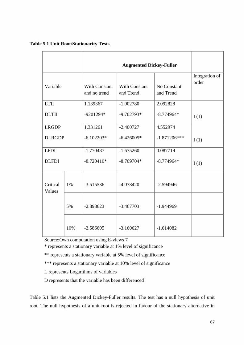
67

Table 5.1 Unit Root/Stationarity Tests

Augmented Dickey-Fuller

Variable

With Constant

and no trend

With Constant

and Trend

No Constant

and Trend

Integration of

order

LTII

DLTII

1.139367

-9201294*

-1.002780

-9.702793*

2.092828

-8.774964*

I (1)

LRGDP

DLRGDP

1.331261

-6.102203*

-2.400727

-6.426005*

4.552974

-1.871206***

I (1)

LFDI

DLFDI

-1.770487

-8.720410*

-1.675260

-8.709704*

0.087719

-8.774964*

I (1)

Critical

Values

1%

-3.515536

-4.078420

-2.594946

5%

-2.898623

-3.467703

-1.944969

10%

-2.586605

-3.160627

-1.614082

Source:Own computation using E-views 7

* represents a stationary variable at 1% level of significance

** represents a stationary variable at 5% level of significance

*** represents a stationary variable at 10% level of significance

L represents Logarithms of variables

D represents that the variable has been differenced

Table 5.1 lists the Augmented Dickey-Fuller results. The test has a null hypothesis of unit

root. The null hypothesis of a unit root is rejected in favour of the stationary alternative in

68

each case if the test statistic is more negative than the critical value. Therefore, a rejection of

the null hypothesis means that the series does not have a unit root. It should also be noted that

the tests were carried out with no constant and trend, with constant but no trend, with both

trend and constant. The unit root using constant and trend suggests that all series become

stationary after first differencing.

The results show that LTII is not stationary in levels in the ADF but does however become

stationary after it has been differenced. The t-statistic -9.702793 becomes bigger than the one

percent critical value -4.078420. When the test is applied to first differences of the series, all

variables become stationary, which suggests that they are all I(1). The null hypothesis of unit

root is therefore rejected and the alternative of no unit root in the series is accepted. The unit

root test using constant and trend assumption shows the most robust results.

The results show that LRGDP is not stationary in all levels but becomes stationary after it has

been differenced. The t-statistic -6.426005 is greater than the Mackinnon value which is -

4.078420 significant at one percent. The null hypothesis of unit root is therefore rejected and

the alternative of no unit root in the series is accepted. The unit root test using constant and

trend assumption shows the most robust results. LFDI was found not stationary in all levels

but becomes stationary when it is first differenced. This is because the ADF t-statistic -

8.774964 is bigger than the one percent Mackinnon value -2.594946. The null hypothesis of

unit is rejected in favour of the alternative hypothesis and the variables are all integrated of

the order I(1).

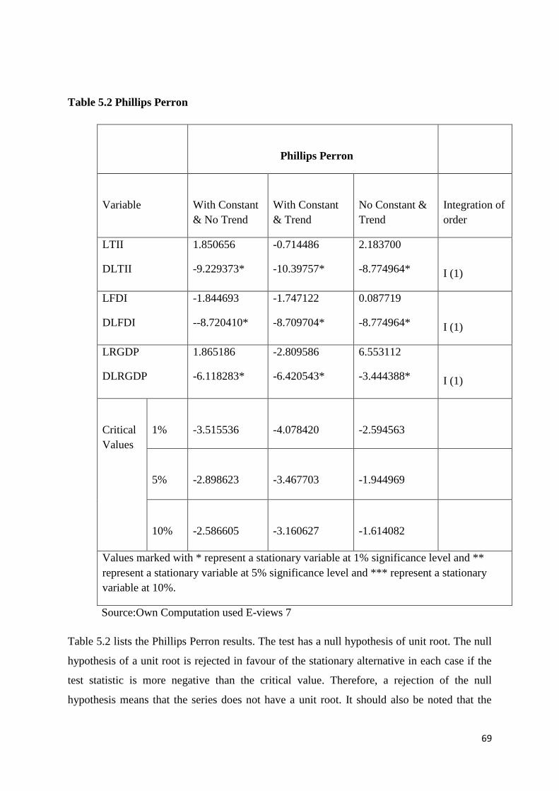
69

Table 5.2 Phillips Perron

Phillips Perron

Variable

With Constant

& No Trend

With Constant

& Trend

No Constant &

Trend

Integration of

order

LTII

DLTII

1.850656

-9.229373*

-0.714486

-10.39757*

2.183700

-8.774964*

I (1)

LFDI

DLFDI

-1.844693

--8.720410*

-1.747122

-8.709704*

0.087719

-8.774964*

I (1)

LRGDP

DLRGDP

1.865186

-6.118283*

-2.809586

-6.420543*

6.553112

-3.444388*

I (1)

Critical

Values

1%

-3.515536

-4.078420

-2.594563

5%

-2.898623

-3.467703

-1.944969

10%

-2.586605

-3.160627

-1.614082

Values marked with * represent a stationary variable at 1% significance level and **

represent a stationary variable at 5% significance level and *** represent a stationary

variable at 10%.

Source:Own Computation used E-views 7

Table 5.2 lists the Phillips Perron results. The test has a null hypothesis of unit root. The null

hypothesis of a unit root is rejected in favour of the stationary alternative in each case if the

test statistic is more negative than the critical value. Therefore, a rejection of the null

hypothesis means that the series does not have a unit root. It should also be noted that the

70

tests were carried out with no constant and trend, with constant but no trend, with both trend

and constant. The unit root using constant and trend suggests that all series become stationary

after first differencing.

The results show that LTII is not stationary in levels but does however becomes stationary

after it has been differenced. The t-statistic 10.39757 becomes bigger than the one percent

critical value -4.078420. When the test is applied to first differences of the series, all

variables become stationary, which suggests that they are all I(1). The null hypothesis of unit

root is therefore rejected and the alternative of no unit root in the series is accepted. The unit

root test using constant and trend assumption shows the most robust results.

The results show that LRGDP is not stationary in all levels but becomes stationary after it has

been differenced. The t-statistic -6.420543 is greater than the Mackinnon value which is -

4.078420 significant at one percent. The null hypothesis of unit root is therefore rejected and

the alternative of no unit root in the series is accepted. The unit root test using constant and

trend assumption shows the most robust results. LFDI was found not stationary in all levels

but becomes stationary when it is first differenced. This is because the t-statistic -8.774964 is

bigger than the one percent Mackinnon value -2.594563. The null hypothesis of unit root is

rejected in favour of the alternative hypothesis and the variables are all integrated of the order

I(1).

5.3 Cointergration

In order to test for Cointergration it is important to test for lag length. The procedure involved

specifying the optimal leg length and choosing the deterministic assumption that the Johansen

test requires. Table 5.3, shows the lag length criteria obtained from the unrestricted VAR.

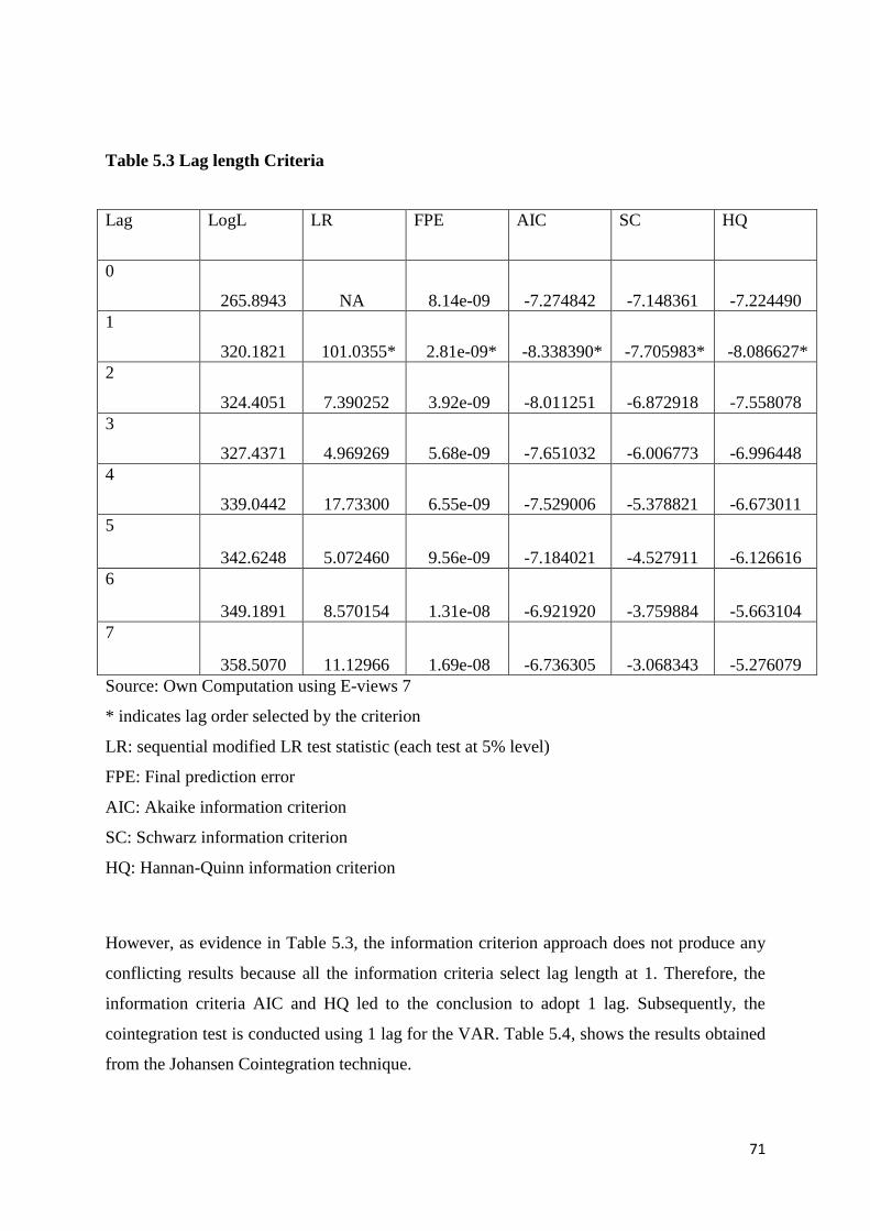
71

Table 5.3 Lag length Criteria

Lag LogL LR FPE AIC SC HQ

0

265.8943 NA 8.14e-09 -7.274842 -7.148361 -7.224490

1

320.1821 101.0355* 2.81e-09* -8.338390* -7.705983* -8.086627*

2

324.4051 7.390252 3.92e-09 -8.011251 -6.872918 -7.558078

3

327.4371 4.969269 5.68e-09 -7.651032 -6.006773 -6.996448

4

339.0442 17.73300 6.55e-09 -7.529006 -5.378821 -6.673011

5

342.6248 5.072460 9.56e-09 -7.184021 -4.527911 -6.126616

6

349.1891 8.570154 1.31e-08 -6.921920 -3.759884 -5.663104

7

358.5070 11.12966 1.69e-08 -6.736305 -3.068343 -5.276079


* indicates lag order selected by the criterion

LR: sequential modified LR test statistic (each test at 5% level)

FPE: Final prediction error

AIC: Akaike information criterion

SC: Schwarz information criterion

HQ: Hannan-Quinn information criterion

However, as evidence in Table 5.3, the information criterion approach does not produce any

conflicting results because all the information criteria select lag length at 1. Therefore, the

information criteria AIC and HQ led to the conclusion to adopt 1 lag. Subsequently, the

cointegration test is conducted using 1 lag for the VAR. Table 5.4, shows the results obtained

from the Johansen Cointegration technique.

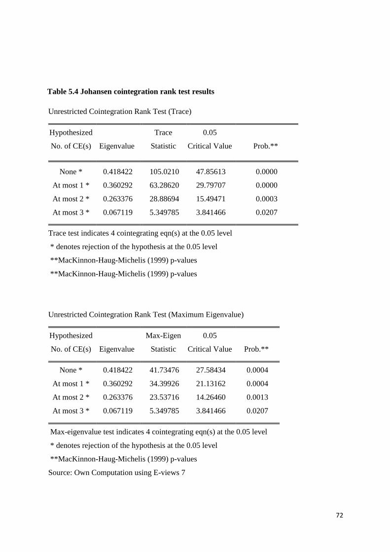
72

Table 5.4 Johansen cointegration rank test results

Unrestricted Cointegration Rank Test (Trace)

Hypothesized Trace 0.05

No. of CE(s) Eigenvalue Statistic Critical Value Prob.**

None * 0.418422 105.0210 47.85613 0.0000

At most 1 * 0.360292 63.28620 29.79707 0.0000

At most 2 * 0.263376 28.88694 15.49471 0.0003

At most 3 * 0.067119 5.349785 3.841466 0.0207

Trace test

indicates 4

cointegrating

eqn(s) at the

0.05 level

Trace test indicates 4 cointegrating eqn(s) at the 0.05 level

* denotes rejection of the hypothesis at the 0.05 level

**MacKinnon-Haug-Michelis (1999) p-values


Unrestricted Cointegration Rank Test (Maximum Eigenvalue)

Hypothesized Max-Eigen 0.05

No. of CE(s) Eigenvalue Statistic Critical Value Prob.**

None * 0.418422 41.73476 27.58434 0.0004

At most 1 * 0.360292 34.39926 21.13162 0.0004

At most 2 * 0.263376 23.53716 14.26460 0.0013

At most 3 * 0.067119 5.349785 3.841466 0.0207

Max-eigenvalue test indicates 4 cointegrating eqn(s) at the 0.05 level

* denotes rejection of the hypothesis at the 0.05 level



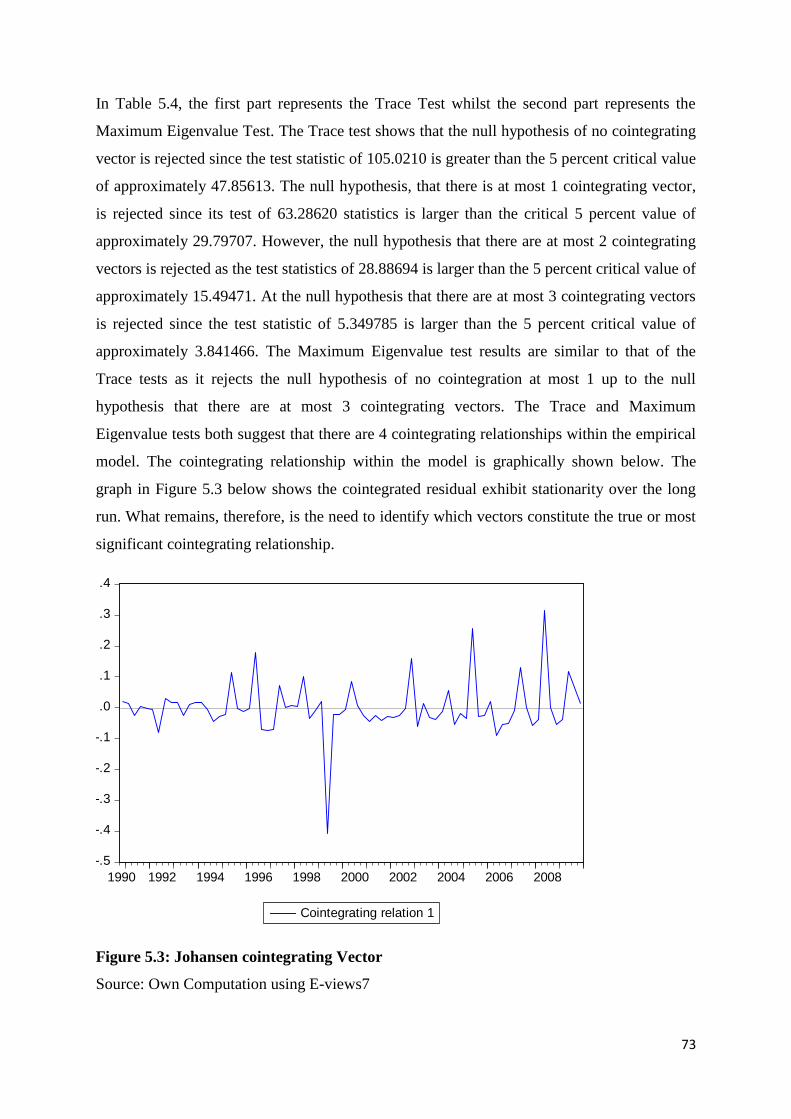
73

In Table 5.4, the first part represents the Trace Test whilst the second part represents the

Maximum Eigenvalue Test. The Trace test shows that the null hypothesis of no cointegrating

vector is rejected since the test statistic of 105.0210 is greater than the 5 percent critical value

of approximately 47.85613. The null hypothesis, that there is at most 1 cointegrating vector,

is rejected since its test of 63.28620 statistics is larger than the critical 5 percent value of

approximately 29.79707. However, the null hypothesis that there are at most 2 cointegrating

vectors is rejected as the test statistics of 28.88694 is larger than the 5 percent critical value of

approximately 15.49471. At the null hypothesis that there are at most 3 cointegrating vectors

is rejected since the test statistic of 5.349785 is larger than the 5 percent critical value of

approximately 3.841466. The Maximum Eigenvalue test results are similar to that of the

Trace tests as it rejects the null hypothesis of no cointegration at most 1 up to the null

hypothesis that there are at most 3 cointegrating vectors. The Trace and Maximum

Eigenvalue tests both suggest that there are 4 cointegrating relationships within the empirical

model. The cointegrating relationship within the model is graphically shown below. The

graph in Figure 5.3 below shows the cointegrated residual exhibit stationarity over the long

run. What remains, therefore, is the need to identify which vectors constitute the true or most

significant cointegrating relationship.

Figure 5.3: Johansen cointegrating Vector

Source: Own Computation using E-views7

-.5

-.4

-.3

-.2

-.1

.0

.1

.2

.3

.4

1990 1992 1994 1996 1998 2000 2002 2004 2006 2008

Cointegrating relation 1

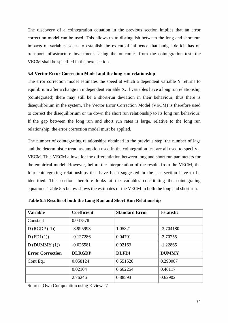
74

The discovery of a cointegration equation in the previous section implies that an error

correction model can be used. This allows us to distinguish between the long and short run

impacts of variables so as to establish the extent of influence that budget deficit has on

transport infrastructure investment. Using the outcomes from the cointegration test, the

VECM shall be specified in the next section.

5.4 Vector Error Correction Model and the long run relationship

The error correction model estimates the speed at which a dependent variable Y returns to

equilibrium after a change in independent variable X. If variables have a long run relationship

(cointegrated) there may still be a short-run deviation in their behaviour, thus there is

disequilibrium in the system. The Vector Error Correction Model (VECM) is therefore used

to correct the disequilibrium or tie down the short run relationship to its long run behaviour.

If the gap between the long run and short run rates is large, relative to the long run

relationship, the error correction model must be applied.

The number of cointegrating relationships obtained in the previous step, the number of lags

and the deterministic trend assumption used in the cointegration test are all used to specify a

VECM. This VECM allows for the differentiation between long and short run parameters for

the empirical model. However, before the interpretation of the results from the VECM, the

four cointegrating relationships that have been suggested in the last section have to be

identified. This section therefore looks at the variables constituting the cointegrating

equations. Table 5.5 below shows the estimates of the VECM in both the long and short run.

Table 5.5 Results of both the Long Run and Short Run Relationship

Variable Coefficient Standard Error t-statistic

Constant 0.047578

D (RGDP (-1)) -3.995993 1.05821 -3.704180

D (FDI (1)) -0.127286 0.04701 -2.70755

D (DUMMY (1)) -0.026581 0.02163 -1.22865

Error Correction DLRGDP DLFDI DUMMY

Cont Eq1 0.058124 0.551528 0.290087

0.02104 0.662254 0.46117

2.76246 0.88593 0.62902


75

The results in Table 5.5 suggest that there is a positive and statistically insignificant

relationship between a budget deficit and transport infrastructure investment in South Africa

during the period reviewed, with a t-statistic of 0.62902. However, in a long run the results

suggest at negative and statistically insignificant relationship between a budget deficit and

infrastructure investment in South Africa during the same period under review. The t-statistic

for this coefficient is -1.22865 at 1 percent significance interval pertaining that a percentage

increase in budget deficit lagged once leads to a decrease in the transport infrastructure

investment. This means that a persistent deficit causes a downward pressure on transport

infrastructure expenditure. According to Moudud (1998), increases in government deficit

tend to lead to a decline in investments which results in crowding out effects. Therefore, an

expansionary government deficit lowers the bond prices, raises the interest rate of bonds,

increases the demand for consumption and, lastly, raises the demand for money. A rise in a

budget deficit leads to a crowd-out effect because it increases the interest rate which later

negatively affects the investment and economic growth.

With respect to FDI, the results suggest a positive and statistically insignificant relationship

between FDIs and transport infrastructure investment in South Africa during the period under

review, with a t-statistic of 0.88593. However, in the long run there is a negative and

statistically significant relationship between FDIs and transport infrastructure investment in

South Africa with a t-statistic of -2.70755. Investment in transport infrastructure including

roads, rail to transport goods is a catalyst in attracting foreign direct investment (SAIIA,

2012). Increased FDI flows into South Africa are the outcome of more public sector

investment in economic infrastructure so as to facilitate more investment by local private

firms. Such increased investment increases confidence in the South African economy and

thereby attracts more foreign direct investment. However, in a long run, the results suggest a

decline in public investment in transport infrastructure. This could imply that, in a long run,

transport infrastructural facilities are sufficiently available meaning that the government’s

investment in transport infrastructure starts to diminish.

With regard to RGDP, the results show that there is a statistically significant but positive

relationship between RGDP and transport infrastructure in South Africa, with a t-statistic of

2.76246 under the period reviewed. However, in the long run there is a statistically

significant but negative relationship between RGDP and transport infrastructure investment

in South Africa, with a t-statistic of -3.74180. This can be explained by the fact that, in a long

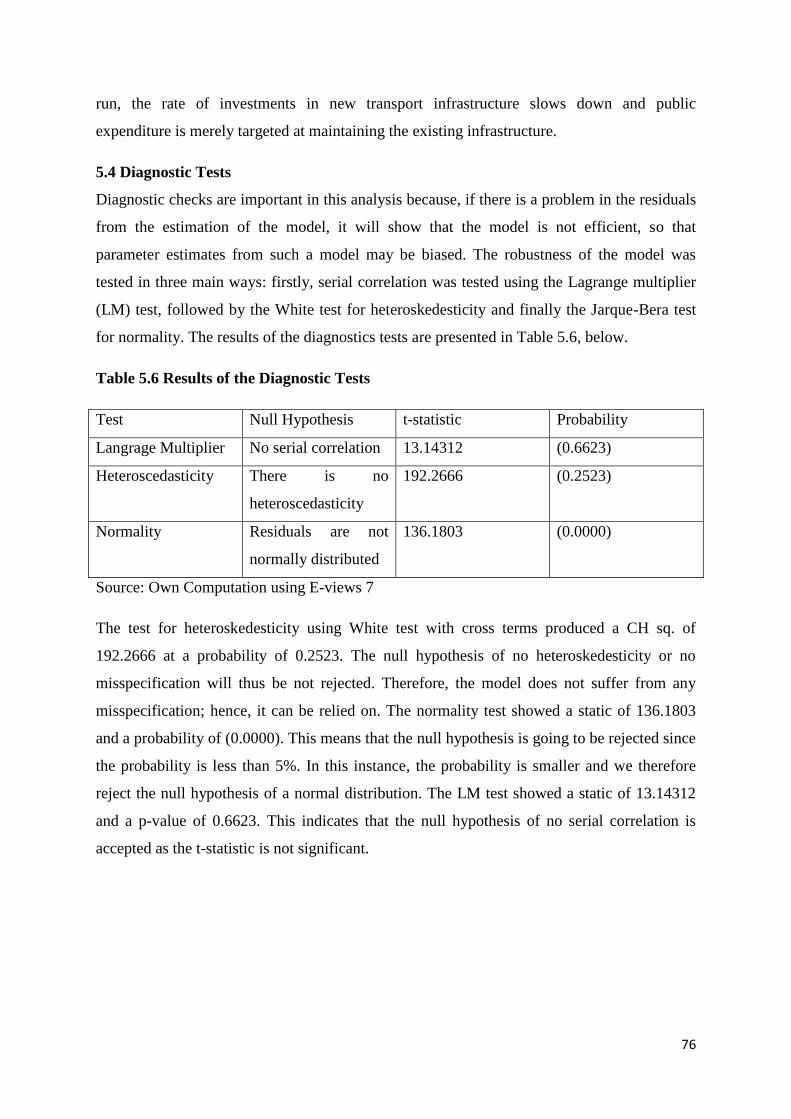
76

run, the rate of investments in new transport infrastructure slows down and public

expenditure is merely targeted at maintaining the existing infrastructure.

5.4 Diagnostic Tests

Diagnostic checks are important in this analysis because, if there is a problem in the residuals

from the estimation of the model, it will show that the model is not efficient, so that

parameter estimates from such a model may be biased. The robustness of the model was

tested in three main ways: firstly, serial correlation was tested using the Lagrange multiplier

(LM) test, followed by the White test for heteroskedesticity and finally the Jarque-Bera test

for normality. The results of the diagnostics tests are presented in Table 5.6, below.

Table 5.6 Results of the Diagnostic Tests

Test Null Hypothesis t-statistic Probability

Langrage Multiplier No serial correlation 13.14312 (0.6623)

Heteroscedasticity There is no

heteroscedasticity

192.2666 (0.2523)

Normality Residuals are not

normally distributed

136.1803 (0.0000)


The test for heteroskedesticity using White test with cross terms produced a CH sq. of

192.2666 at a probability of 0.2523. The null hypothesis of no heteroskedesticity or no

misspecification will thus be not rejected. Therefore, the model does not suffer from any

misspecification; hence, it can be relied on. The normality test showed a static of 136.1803

and a probability of (0.0000). This means that the null hypothesis is going to be rejected since

the probability is less than 5%. In this instance, the probability is smaller and we therefore

reject the null hypothesis of a normal distribution. The LM test showed a static of 13.14312

and a p-value of 0.6623. This indicates that the null hypothesis of no serial correlation is

accepted as the t-statistic is not significant.

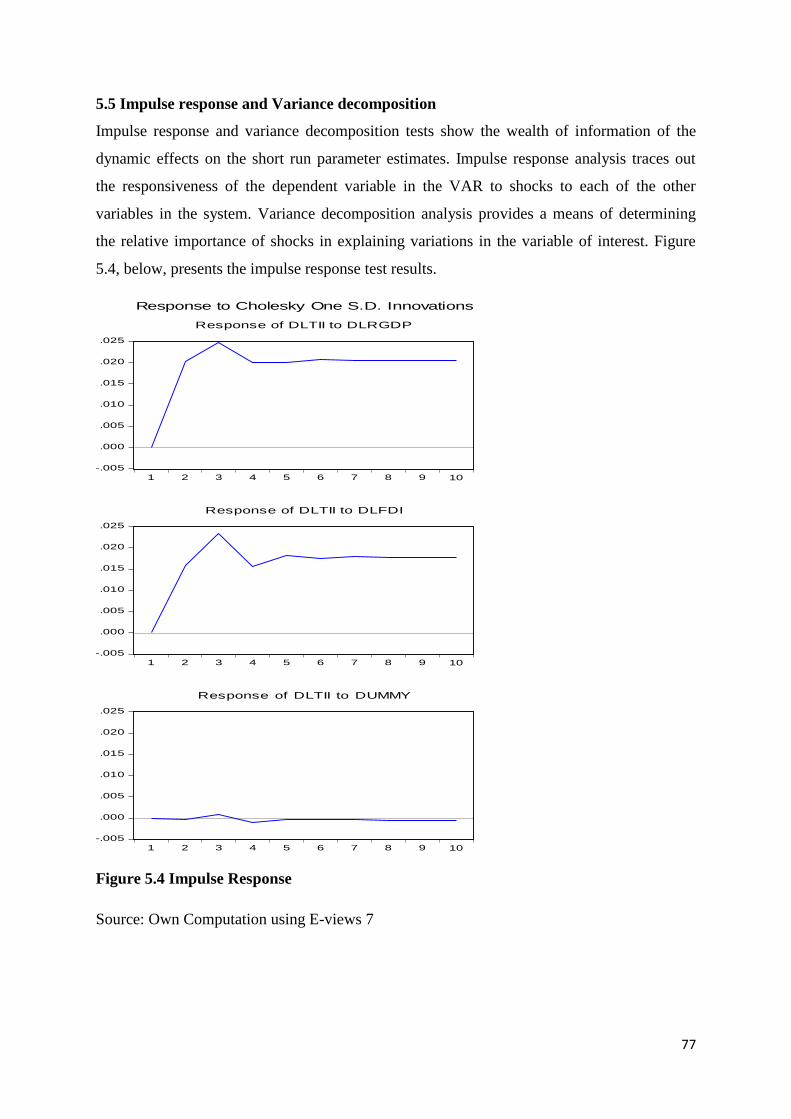
77

5.5 Impulse response and Variance decomposition

Impulse response and variance decomposition tests show the wealth of information of the

dynamic effects on the short run parameter estimates. Impulse response analysis traces out

the responsiveness of the dependent variable in the VAR to shocks to each of the other

variables in the system. Variance decomposition analysis provides a means of determining

the relative importance of shocks in explaining variations in the variable of interest. Figure

5.4, below, presents the impulse response test results.

Figure 5.4 Impulse Response


-.005

.000

.005

.010

.015

.020

.025

1 2 3 4 5 6 7 8 9 10

Response of DLTII to DLRGDP

-.005

.000

.005

.010

.015

.020

.025

1 2 3 4 5 6 7 8 9 10

Response of DLTII to DLFDI

-.005

.000

.005

.010

.015

.020

.025

1 2 3 4 5 6 7 8 9 10

Response of DLTII to DUMMY

Response to Cholesky One S.D. Innovations

78

These impulse response functions show the dynamic response of the transport infrastructure

investment to a one-period standard deviation shock to the innovations of the system and

indicate the directions and persistence of the response to each of the shocks over a 10 quarter

(2.5years) period. For the most part, the impulse response functions have the expected pattern

and confirm the results from the short run relationship. The first graph shows the response of

the independent variable to deviations by itself; this simply means that the effect or

responsiveness of transport infrastructure investment to changes in transport infrastructure

investment. The transport infrastructure investment had decreased in the second quarter for a

short run period but remained stable throughout the 10 quarter period. A one time period

standard deviation shock to RGDP the effect is stable but starts to appreciate in the second

quarter and starts to decrease until it reaches a stable state in the fourth quarter till the 10th

quarter. The effect of RGDP to TII explains the high coefficient and affects it in the long run.

A onetime standard deviation shock to FDI marginally decreases the TII in the fifth quarter

through-out the last quarter. Among all the analysed variables only RGDP is shown to have a

persistent and significant impact on transport infrastructure investment and conforms to the

results obtained, the rest seems to show a negative impact on transport infrastructure

investment.

5.6 Variance Decomposition

Variance decomposition analysis provides for a means of determining the relative importance

of shocks in explaining variations in the variable of interest. In the context of this study, it

therefore provides a way of determining the relative importance of shocks to each of the

budget deficits in explaining variations in transport infrastructure investment. The results of

the variance decomposition analysis are presented in Table 5.7 and these show the proportion

of the forecast error variance in transport infrastructure investment explained by its own

innovations and innovations in the budget deficit.

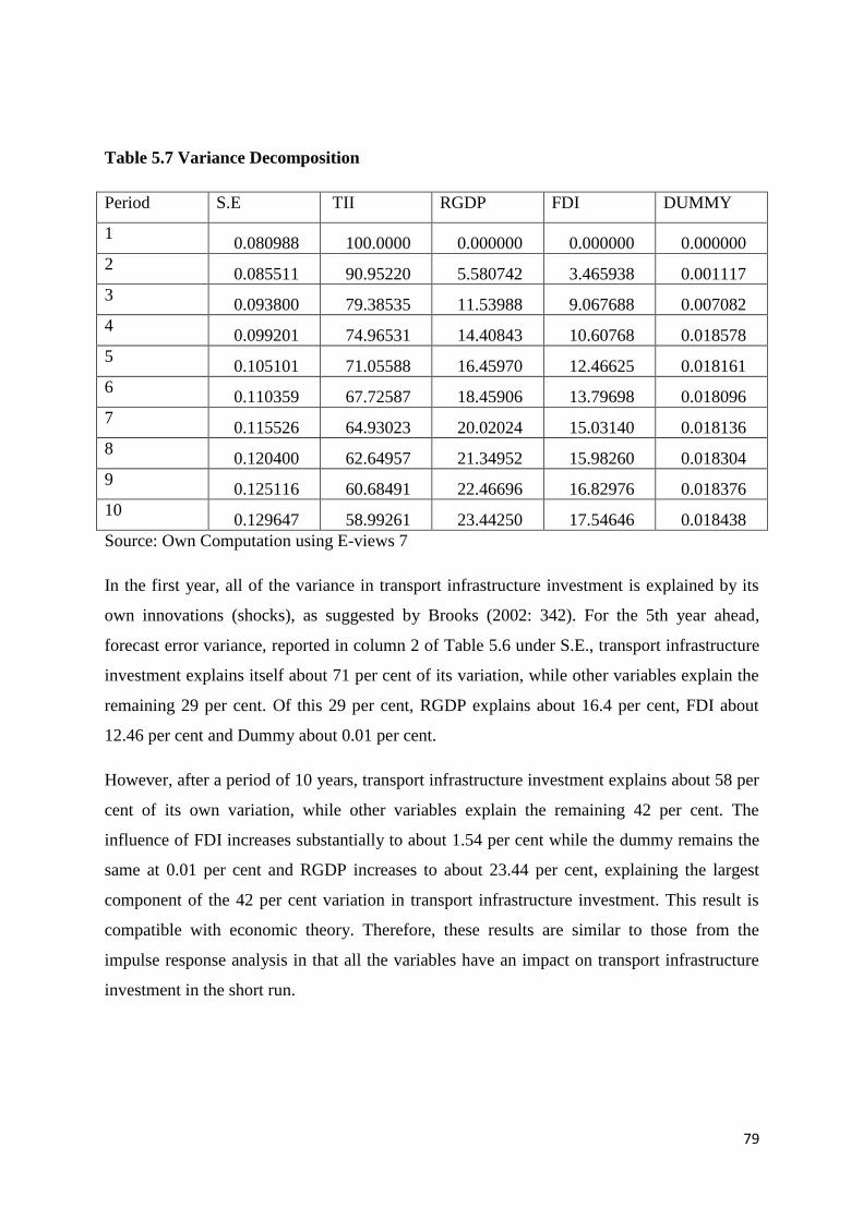
79

Table 5.7 Variance Decomposition

Period S.E TII RGDP FDI DUMMY

1 0.080988 100.0000 0.000000 0.000000 0.000000

2 0.085511 90.95220 5.580742 3.465938 0.001117

3 0.093800 79.38535 11.53988 9.067688 0.007082

4 0.099201 74.96531 14.40843 10.60768 0.018578

5 0.105101 71.05588 16.45970 12.46625 0.018161

6 0.110359 67.72587 18.45906 13.79698 0.018096

7 0.115526 64.93023 20.02024 15.03140 0.018136

8 0.120400 62.64957 21.34952 15.98260 0.018304

9 0.125116 60.68491 22.46696 16.82976 0.018376

10 0.129647 58.99261 23.44250 17.54646 0.018438


In the first year, all of the variance in transport infrastructure investment is explained by its

own innovations (shocks), as suggested by Brooks (2002: 342). For the 5th year ahead,

forecast error variance, reported in column 2 of Table 5.6 under S.E., transport infrastructure

investment explains itself about 71 per cent of its variation, while other variables explain the

remaining 29 per cent. Of this 29 per cent, RGDP explains about 16.4 per cent, FDI about

12.46 per cent and Dummy about 0.01 per cent.

However, after a period of 10 years, transport infrastructure investment explains about 58 per

cent of its own variation, while other variables explain the remaining 42 per cent. The

influence of FDI increases substantially to about 1.54 per cent while the dummy remains the

same at 0.01 per cent and RGDP increases to about 23.44 per cent, explaining the largest

component of the 42 per cent variation in transport infrastructure investment. This result is

compatible with economic theory. Therefore, these results are similar to those from the

impulse response analysis in that all the variables have an impact on transport infrastructure

investment in the short run.

80

5.7 Conclusion

The first section presented the unit root test where the Augmented Dickey-Fuller and Phillips

Perron tests were used to test for stationarity. Both methods revealed that the data series are

non-stationary in levels and stationary when first differenced. Therefore, the series are

integrated of the same order I (1).

Cointegration tests were presented in the second section where the lag order information

criteria approach was applied as a direction in choosing the lag order. 1 lag was used in order

to permit adjustments in the model and accomplish well behaved residuals. All the

information criteria approaches used selected 1 lag; therefore, a conclusion to adopt 1 lag for

VAR was made. The Johansen cointegration tests provided evidence that there is no

cointegration between transport infrastructure investment and the explanatory variables.

The short run dynamics are not consistent with literature showing the Foreign Direct

Investment, RGDP have a negative impact on TII while the budget deficit shows consistent

results of having a negative effect on TII. The impulse response showed that RGDP is the

only variable that has been persistent on TII whilst variance decomposition showed that all

the variables have an impact on transport infrastructure investment in the short run, but the

RGDP has the most significant effect followed by the FDI and the budget deficit.

The last section of this chapter presented the results of the diagnostic checks, impulsive

response and variance decomposition. Diagnostic checks revealed the suitability of the

model; there is serial correlation and no misspecification while the errors are normally

distributed. Both the impulse response and variance decomposition produced results that are

compatible with economic theory. Therefore, the results from this research can be relied

upon. Compelling conclusions on the impact of budget deficit and transport infrastructure

investment can be deduced and applicable policies can be safely formulated. The summary of

the main findings, conclusions and recommendations are presented in the ensuing chapter.

81

CHAPTER SIX

SUMMARY OF THE MAIN FINDINGS, CONCLUSIONS, IMPLICATIONS AND

RECOMMENDATIONS

6.1 Summary of the study and conclusions

The main objective of this research was to assess the impact of a budget deficit on transport

infrastructure investment in South Africa. The objective of this study was addressed by

looking at all the aspects contributing towards budget deficits. These aspects include the

financial crisis, debts and increasing social welfare expenditure. This chapter begins by

presenting some highlights of each chapter, which is followed by conclusions. The last part of

the chapter offers a set of policy recommendations based on the findings of this study.

The first chapter outlined that the aim of the study, its objectives, problem statement and the

significance of the study. Chapter Two presented an analysis of the theoretical and empirical

literature pertinent to the study. In the main, this chapter presented a literature review on

growth theories; namely, the Harrod-Domar, neo-classical and endogenous growth models.

Based on the discussion of growth theories, this study adopted endogenous growth models as

a theoretical framework for this study.

Chapter Three presented an overview of the variables included in the econometric model

used to analyse the data in this study. In this regard, trends on transport infrastructure

investment, gross domestic product, foreign direct investment as well as a budget balance

during the period under review was presented.

Chapter Four presents the research methodology employed in this study. The study is based

on quantitative research techniques using econometric analysis. Specifically, the time series

data covering the period 1990 to 2009 (quarterly data) was analysed using a vector error

correction model. All the methodological steps used in analysing the data were outlined in

Chapter Four; this includes stationarity tests, tests for cointegration and diagnostic tests, all of

which were explained in this chapter.

Chapter Five presents the analysis of data and the results of the analysis. The main findings

of this analysis show that a budget deficit negatively impacts investments in transport

82

infrastructure in South Africa, during the period under review. Based on these findings, the

results suggest that a null hypothesis presented in chapter one of this study cannot be rejected.

6.2 Conclusions

The results from the analysis of the variables included in the econometric estimation model

show that the variations in transport infrastructure investment are mainly explained by

economic growth followed by foreign direct investment and, lastly, by a budget deficit. The

main insight that can be drawn from this analysis is that a budget deficit has a negative

impact on transport infrastructure investment in the long run. The findings show that the

budget deficit is consistent in both the short and the long run negatively affecting transport

infrastructure investments. With the budget deficit increasing it does not only affect the

transport infrastructure investments but it also lowers the bond prices, raises the interest rates

and has a crowding-out effect.

6.3 Recommendations

Based on the results of this study, the following recommendations are provided:

In order to ensure that transport infrastructure investment is maintained on a positive

level, foreign direct investments should be attracted. In fact, a good transport

infrastructure on its own attracts foreign direct investments.

Policy makers should ensure that pro-growth policies are devised and implemented in

South Africa. This will help maintain sustainable economic growth in South Africa.

Whilst expansionary fiscal policy is desirable for its economic benefits, the Treasury

should ensure that there is fiscal discipline in the budget. This will help curtail a

budget deficit which will in turn help boost infrastructural investments in South

Africa.

6.4 Delimitations and recommendations for future research

This study focused primarily on data from 1990 to 2009, due to the unavailability of data in

some of the variables. The main thrust of this study is on the impact of a budget deficit and its

impact on transport infrastructure investment. Other factors that may influence transport

infrastructure investment were excluded. For future research the researchers could apply the

same econometric model but use the different period to check how the budget deficit affected

the transport infrastructure investment during the apartheid years.

83

REFERENCES

Abayomi, T. (2011). Government expenditure and economic development: Empirical

evidence from Nigeria. MPRA Paper. University Library of Munich. Germany.

Adam, C.S., Bevan, D.L. (2004). Fiscal deficits and growth in developing countries.

Department of Economics, University of Oxford, Oxford.

Ajam, T and Aron, J. (2007). Transforming Fiscal Governance. Department of Economics,

University of Oxford, Oxford.

Al-Khedair, S.I. (1996). The Impact of the Budget Deficit on Key Macroeconomic

variables in the Major Industrial Countries. PhD Dissertation, Florida Atlantic

University.

Anayochukwu, O.B. (2012). Fiscal Deficits and Inflation in Nigeria: The Causality

Approach. International Journal of Scientific & Technology Research Volume 1. Issue 8.

September 2012.

Anušić, Z. (1994). Budget Deficit and Inflation: Croatia in the years 1991 and 1992.

Ekonomski pregled, Zagreb, Vol. 7. No. 8.

Arrow, K, J & Kurz, M. (1970). Public Investment, Rate of Return and the Optimal

Fiscal Policy. Johns Hopkins University Press, Baltimore.

Arrow, K. J., Dasgupta, P. & Maler, K.G. (2003). The Genuine Savings Criterion and The

Value of Population. Economic Theory. Springer-Verlag.

Aschauer, D.A. (1985). Fiscal Policy and Aggregate Demand. American Review

Association. Vol (75). No (1).pp. 117-127.

Aschauer, D.A. (1989). Is Public Expenditure Productive. Journal of Monetary Economics.

Federal Reserve Bank of Chicago. pp. 177-200. North Holland.

Aschauer, D.A. (1989b). Does Public Capital Crowding Out Private Capital. Federal

Reserve Bank of Chicago Staff Memoranda.

Ball, L. and Mankiw, N.G. (1995). What Do Budget Deficits Do?.Federal Reserve Bank of

Kansas City.

Barro, R. (1987). Government Spending, Interest Rates, Prices and Budget Deficits in

the United Kingdom. Journal of Monetary Economics No (20). pp. 221-247

Barro, R. (1990). Government Spending in a Simple Model of Endogenous Growth.

Journal of Political Economy. 98(5), S103-S125.

Barro, R. and Grilli, V. (1994). European Macroeconomics. Ch.15-16. Macmillan.London

84

Bassanini, A., & Scarpetta, S. (2002). Growth, technological change and ICT diffusion:

Evidence form OECD countries. Oxford Review of Economic Policy, 18 (3): 324-344.

Bhorat, H. & Oosthuizen, M., (2005). The Post-Apartheid South African Labour Market.

DPRU Working Paper, No 05/923, Cape Town.

Bonga-Bonga, L. (2011). Budget deficit and long term interest rates in South Africa.

Department of Economics and Econometrics. University of Johannesburg.

Bosch, N. and Espasa, M. (1999). The central public sector transport infrastructure

investment deficit in Catalonia and future prospects. Barcelona Institute of Economics.

University of Barcelona.

Bose, N., Haque, M.E. and Osborn, D.R. (2007). Public expenditure and economic growth:

A disaggregated analysis for developing countries. Centre for Growth and Business Cycle

Research Discussion Paper Series. The Manchester School.75(5):533-556.

Brooks, C. (2003). Introductory Econometrics for Finance. Cambridge University

Burda, M. and Wyploszy, C. (2001). Macroeconomics: A European Text (3e). New York:

Oxford University Press.

Chakraborty, L.S. (2002). Fiscal Deficit and Rate of Interest: An Econometric Analysis of

the Deregulated Financial Regime. Economic and Political Weekly, 37(19).

Chmura Economics and Analytics. (2011). Economic and Fiscal Impacts of the

Construction Phase of Transportation Funding in Virginia and its Regions. Virginia.

Cogito. (2010). How Budget Deficit Affects Economic Growth? Word Press.com. [Online]

Available: http://qmarks.wordpress.com/2010/page/55/. (Accessed 20 November 2012).

Cohen, R. and Percoco, M. (2003). The Fiscal Implications of Infrastructure

Development. Bocconi University. Washington DC.

Copeland, C., Levine, L. and Mallet, W.J. (2011). The Role of Public Works

Infrastructure in Economic Recovery. Congressional Research Service

Du Plessis S. and Smit B., (2007). South Africa’s growth revival after 1994. Stellenbosch

Economic Working Papers: 01/06.

Easterly, W. and Hebbel K.S. (1992). Fiscal Adjustment and Macroeconomic

Performance: A Synthesis. Published for the World Bank. New York University Press.

Economics, 22: 3-42.

Ernst and Young. (2009-2012). Repositioning the South African Investment Case. Africa

Business Center. EYGM Limited.

Fatas, A. and Muhov, I. (2001). The Effects of Fiscal Policy on Consumption and

Employment: Theory and Evidence. CEPR Discussion Paper No. 2760.

http://qmarks.wordpress.com/2010/page/55/

85

Fatima, G., Ahmed, A.M. and Rehman, U.W. (2011). Fiscal Deficit and Economic Growth:

An Analysis of Pakistan’s Economy. International Journal of Trade, Economics and

Finance, Vol. 2, No. 6, December 201.

Fatima, G., Ahmed, A.M. and Rehman, U.W. (2012). Consequential Effects of Budget

Deficit on Economic Growth of Pakistan. International Journal of Business and Social

Science Vol. 3 No. 7.

Fedderke, J. and Garlick, R. (2008). Infrastructure Development and Economic Growth

in South Africa: A Review of the Accumulated Evidence. University of Cape Town.

Policy Paper No (12).

Fedderke, J. Perkins, P. and Luiz, J. (2005). Infrastructure Investment in Long Run

Economic Growth: South Africa 1875-2001. Preliminary Draft. [Online] Available:

http://www.uct.ac.za/economics. (Accessed 29 March 2012).

Fedderke, J. W., & Simkins, C. (2006). Economic Growth in South Africa since the late

nineteenth Century. Available:

www.commerce.uct.ac.za/economics/staff/jfedderke/.../ross.pdf. (Accessed 21 June 2013).

Fourie, J. (2006). A Review of Economic Infrastructure in South Africa. Masters

dissertation in partial fulfilment of the degree M.Comm Economics at the University of

Stellenbosch.

Georgantopoulos, A.G. and Tsamis, A.D. (2011). The Macroeconomic Effects of Budget

Deficits in Greece. International Research Journal of Finance and Economics - Issue 79

Ghali, K., & Al-Shamsi, F. (1997). Fiscal Policy and Economic Growth: A study Relating

to the United Arab Emirates. Economies International, 50, 519-533.

Goyal, R. (2004). Does Higher Fiscal Deficit Lead to Rise in Interest Rates? Economic

and Political Weekly 39(21): 2128–33.

Grant-Muller, S. and Laird, J. (2006). Costs of Congestion: Literature Based Review of

Methodologies and Analytical Approaches. Edinburgh. Scottish Executive.

Gujarati, D.N. (2003). Basic econometrics. 4th edition. New York. McGraw-Hill.

Gulcan, Y. and Bilman, M.E. (2005). The Effects of Budget Deficit Reduction on

Exchange Rate: Evidence from Turkey. Discussion Paper Series 05/07, Dokuz Eylül

University, Faculty of Business, Department of Economics.

Hadiwibowo, Y. (2010). Fiscal Policy, Investment and Long-Run Economic Growth:

Evidence from Indonesia. Graduate School for International Development and Cooperation,

Hiroshima University 1-5-1 Kagamiyama, Higashi-Hiroshima, Hiroshima, 739-8529, Japan

Hakkio, C.S. (1996). The Effects of Budget Deficit Reduction on the Exchange Rate.

Economic Review (Federal Reserve Bank of Kansas City), 81, 21-38.

http://www.uct.ac.za/economics

http://www.commerce.uct.ac.za/economics/staff/jfedderke/.../ross.pdf

86

Harris, R. (1995). Using Cointegration Analysis in Econometric Modelling. Prentice Hall.

London.

Harrod, R. (1939). An Essay in Dynamic Theory. The Economic Journal. Vol (49). No

(193)

International Transport Forum. (2012). Measuring Investment in Transport

Infrastructure. International Energy Agency. [Online] Available:

http://www.internationaltransportforum.org/Proceedings/InfrastructureInv/Investment%20wo

rkshop%20programme. (Accessed 25 November 2012).

Johansen, S. and Juselius K. (1990). The full information maximum likelihood procedure

for inference on cointegration-with applications to the demand for money. Oxford

Bulletin of Economics and Statistics Vol 52 pg 169-210

Johansen, S. (1991). Estimation and hypothesis testing of co-integration vectors in

Gaussian vector autoregressive models. Econometrica Vol 59 pg 1551-1580

Johansen, S., (1995). Likelihood-based inference in cointegrated vector autoregressive

models. Oxford University Press. Western Hemisphere.

Joharji, G.A. and Starr, M.A. (2012). Fiscal policy and growth in Saudi Arabia.

Department of Economics: Washington, DC.

Jooste, C., Liu, G. and Naraidoo, R. (2012). Analysing the Effects of Fiscal Policy Shocks

in the South African Economy. Department of Economics Working Paper Series.

University of Pretoria.

Joshi, V. (2009). Fiscal Policy in Macroeconomics. Washington, DC.

Kasende, L. Brixova, Z. and Ndikumana, L. (2010). Africa: Africa’s Counter Cyclical

Fiscal Policy Responses to the Crisis. Journal of Globalization and Development. 1(1) pp.

22–28.

Khaliq, A. and Noy, I. (2007). Foreign Direct Investment and Economic Growth:

Empirical Evidence from Sectoral Data in Indonesia. Department of Economics. Andalas

University, Indonesia.

Khamfula, Y. (2004). Macroeconomic Policies, Shocks and Economic Growth in South

Africa. School of Economic and Business Sciences. University of Witwatersrand.

Khan, A.Q. and Khattak, N.R. (2008). An Analysis of Short-Term Effects of Budget

Deficits on Macroeconomic Variables: Evidence from Pakistan (1960-2005). Sarhad J.

Agric. Vol.24, No.2,

Khinoshita, Y. and Campos, N.F. (2002). Foreign Direct Investment as a Technology

Transferred: Some Panel Evidence from the Transition Economies. William Davidson

Working Paper, No, 438.

http://www.internationaltransportforum.org/Proceedings/InfrastructureInv/Investment%20workshop%20programme.pdf

http://www.internationaltransportforum.org/Proceedings/InfrastructureInv/Investment%20workshop%20programme.pdf

87

Kneller, R., Bleaney, M. and Gemmell, N. (1999). Fiscal Policy and Growth: Evidence

from OECD Countries. Journal of Public Economics, 74, 171-90.

Kumo, W.L. (2012). Infrastructure Investment and Economic Growth in South Africa.

Working Paper Series N° 160 African Development Bank, Tunis.

Kustpeli, Y. (2001). The Effect of Nominal Government Deficits on Economic Growth.

Faculty of Business Department of Economics.

Levy, P. (1999). Sanctions on South Africa: What did they do? Center Discussion Paper

No. 796.

Loots, E. (1998). Job Creation and Economic Growth. South African Journal of

Economics. Vol 66, Issue 3, pg. 155-163.

Lucas, R. (1988). On the Mechanics of Economic Development. Journal of Monetary.

Luintel, K.B., & Khan, M. (1999). A Quantitative Reassessment of the Finance–Growth

Nexus: Evidence from a Multivariate VAR. Journal of Development Economics. 60: 381–

405.

Lütkepohl, H. and Reimers, H.E., (1992). Impulse response analysis of a cointegrated

system. Journal of Economic Dynamics and Control Vol 16 pg 53-78

Lütkepohl, H. (1991). Introduction to multiple time series analysis. New York: Springer-

Verlag.

Mabungu, R and Chitiga, M. (2009). “Public Infrastructure Investment” Annual

Submission on the Division of Revenue, Technical Report 2010-201, 19-41, Financial and

Fiscal Commission.

Mackinnon, J.G. (1991). Critical Values for Cointegration Tests. In: Engle, R.F. and

Granger, C.W.J. (1987). Long-run Economic Relationships. Oxford University Press: Oxford.

Mackinnon, J.G. (1996). Numerical Distribution Functions for Unit Root and

Cointegration Tests. Journal of Applied Econometrics, 11: 601-618.

Mellander, E., Vredin, A., and Warne, A. (1992). Stochastic trends and economic

fluctuations in a small open economy. Journal of Applied Econometrics Vol 7 pg 369-394.

Mlambo-Ngcuka, P. (2006). Accelerated and Shared Growth Initiative for South Africa.

[Online] Available: http: //www.info.gov.za/asgisa/.html. (Accessed 05 April 2012]

Mollentze, S. and Van der Merwe, E. (2010). Monetary economics in South Africa. Cape

Town: Oxford University Press.

Moudud, J.K. (1998). Government Spending and Growth Cycles: Fiscal Policy in a

Dynamic Context. The Jerome Levy Economics Institute.Jerome

88

Moudud, J.K. (1999). Government Spending in a Growing Economy. The Jerome Levy

Economics Institute of Bard College. Jerome.

Mwakalikamo, B. (2011). The Effect of a Budget Deficit on Inflation and Current

Accounts. Department of Economics.

National Treasury (2002). The South African Tax Reform Experience Since 1994.

Address by the Honourable Trevor Manuel, MP, Minister of Finance, Annual Conference of

The International Bar Association.

National Treasury. (1995 – 2013). National Budget Review. [Online] Available

http://www.treasury.gov.za/documents/nationalbudgetreview [Accessed 22 May 2013].

National Treasury. (1995 – 2013). National Budget Speech. [Online] Available

http://www.treasury.gov.za/documents/nationalbudgetspeech [Accessed 19 May 2013].

National Treasury. (1998). Fiscal Policy and the Budget Framework. The Medium Term

Budget Policy Statement.

National Treasury. (2012). Budget Speech. Pretoria.

Nattrass, N. (2000). Macroeconomics: Theory and Policy in South Africa. Second edition.

David Philip, Cape Town.

Negota, G.M. (2001). The impact of transport investment on infrastructure and

economic development: The debate. South Africa, 16–20 July.

Ocran, M.K. (2009). Fiscal Policy and Economic Growth in South Africa. Conference on

Economic Development in Africa. Oxford University. UK.

Odhiambo, O.S., Momanyi, G., Frederick, O.A., and Othuon, L. (2013). The Relationship

between Fiscal Deficits and Economic Growth in Kenya. Greener Journal of Social

Sciences Vol. 3 (6), pp. 306-323, July 2013.

Oladipo S.O. and Akinbobola T.O. (2011). Budget Deficit and Inflation in Nigeria. Journal

of Emerging Trends in Economics and Management Sciences, 2 (1) 1-8

Olomola, P.A. and Olagungu M.A. (2004). Fiscal Deficit and private consumption

behaviour in Nigeria: 1970-2001. The Indian Journal of Economics; Vol. LXXXIV, No

335, Pp 597-607.

Organisation for Economic Co-operation and Development (OECD). (2002). Impact of

Transport Infrastructure Investment on Regional Development. OECD France.

Perkins, P. (2003). An Analysis of Economic Infrastructure Investment in South Africa.

University of Witwatersrand working paper 2003- 04.

Perkins, P., Fedderke, J. and Luiz, J. (2005). An Analysis of Economic Infrastructure

Investment in South Africa. South African Journal of Economics, 73(2), 211-227.

89

Political Information and Monitoring Services. (2013). Revenue Estimation, the budget

balance and fiscal accountability in South Africa. Idasa. Budget Paper.

Rahman, N.H.A. (2012). The Relationship between Budget Deficit and Economic Growth

from Malaysia’s Perspective. International Conference on Economics, Business Innovation

IPEDR vol.38 (2012) IACSIT Press, Singapore.

Raju, S. and Mukherje, J. (2010). Fiscal Deficit, Crowding out and the sustainability of

the Economic Growth: The Case of the Indian Economy.

Ramzan, M., Saleem, S. and Butt, I.M. (2013). Budget Deficit and Economic Growth: A

case Study of Pakistan. Interdisciplinary Journal of Contemporary Research in Business.

Vol. 5, No.1.

Rena, R. and Kefela, G.T. (2011). Restructuring a fiscal policy encourages economic

growth – a case of selected African countries. Journal of Economics and Business. Volume

XIV – 2011, No 2 (23-39).

Reungsri, T. (2010). The impact of public infrastructure investment on economic growth

in Thailand. Victoria University. School of Economics and Finance.

Romer, P. (1986). Increasing Returns and Long-run Growth. Journal of Political

Economy, 94: 1002-37.

Romer, P. (1990). Endogenous Technological Change. Journal of Political Economy, 98

(5): 71-102.

Roy, R., Heuty, A. and Letouzé, E. (2006). Fiscal Space for Public Investments: Towards

a Human Development Approach. United Nations Development Programme. G-24

Technical Meeting Paper. Singapore.

Rutkowski, A. (2009). Public Investment, Transport Infrastructure and Growth in

Poland. European Commission’s Directorate-General for Economic and Financial Affairs.

Vol 6, Issue 11.

SARB (1998–2012). Annual Economic Reports. [Online] Available

http://www.resbank.co.za/Publications/Reports/Documents/Annual Report 2010.pdf

[Accessed 03 March 2013]

Schäuble, F. (2012). Review of the Federal Budget. Spiegel online international. [Online]

Available.http://www.spiegel.de/international/europe/german-finance-minister-schaeuble

says-worst-over-in-euro-crisis-a-874934.html. (Accessed 27 July 2013).

Schoeman, N.J, Robinson, Z.C. and de Wet, T.J. (2000). Foreign Direct Investment Flows

and Fiscal Discipline in South Africa. Department of Economics, University of Pretoria.

Shojai, S. (1999). Budget Deficits and Debt: A Global Perspective. Praeger. USA.

Sill, K. (2005). Do Budget Deficits Cause Inflation? Business Review, 26-33.

90

South African Year Book. (2010). Moving South Africa: A transport Strategy for 2020

Spoehr, J., Burgan, B. and Molloy, S. (2012). Public Investment, Productivity and

Economic Growth- The Role and Contribution of Debt Funding. Australian Institute for

Social Research.

Srivyal, V. and Venkata, S.S. (2004). Budget Deficits and other Macroeconomic Variables

in India. Applied Econometrics and International Development. AEEADE. Vol.4-1.

The World Bank (2013) .Global Economic Prospects: Commodity Markets at the

Crossroads. [Online] Available http://0-go.worldbank.org.wam.seals.ac.za/RWLJPPA0D0

[05 July 2013]

The World Bank. (2013). Infrastructure in Sub-Saharan Africa. Online Available.

http://web.worldbank.org/WBSITE/EXTERNAL/COUNTRIES/AFRICAEXT/0,contentMD

K:21951811~pagePK:146736~piPK:146830~theSitePK:258644,00.html. (Accessed 27 July

2013).

Thirwall, A.P. (2002). Growth and Development with special reference to Developing

Countries. 7th

Edition. Palgrave Macmillan, London.

Tien-Ming, S. and Yuli, S. (2003). The Impact of Budget Deficit on Currency Value: A

Comparison of Asian and European Countries.

Todaro, M.P. and Smith, S.C. (2009). Economic Development. Pearson Addison Wesley.

Trading Economics. (2013). South Africa Government Spending. Online Available:

http://www.tradingeconomics.com/south-africa/government-spending. (Accessed 14 April

2013).

United Nations Conference on Trade and Development. (2004b). Development and

Globalisation. United Nations. New York and Geneva.

United Nations Conference on Trade and Development. (2005). Rethinking the Role of

Foreign Direct Investment. Economic Development in Africa. United Nations. New York

and Geneva.

UWASU, M. (2006). The Solow Growth Model. [Online] Available:

http://www.econ.kuleuven.be.pdf (Accessed 29 June 2012).

Velnampy, T. and Achchuthan, S. (2013). Fiscal Deficit and Economic Growth: A study

on Sri Lankan Economic Perspective. Developing Country Studies. Vol. 3, No. 3.

Venter, A. (2009). Infrastructure Development in South Africa. Faculty of Engineering,

Built Environment and Information Technology. University of Pretoria.

White, H. (1980). A heteroskedasticity-consistent covariance matrix and a direct test for

heteroskedasticity. Econometrica vol 48 pg 817- 838.

http://web.worldbank.org/WBSITE/EXTERNAL/COUNTRIES/AFRICAEXT/0,contentMDK:21951811~pagePK:146736~piPK:146830~theSitePK:258644,00.html

http://web.worldbank.org/WBSITE/EXTERNAL/COUNTRIES/AFRICAEXT/0,contentMDK:21951811~pagePK:146736~piPK:146830~theSitePK:258644,00.html

http://www.tradingeconomics.com/south-africa/government-spending

http://www.econ.kuleuven.be/

91

Yongding, Y. (2010). The Impact of the Global Financial Crisis on the Chinese Economy

and China’s Policy Responses. Third World Network.

Zhan, J. (2009). The Role of Public Investment in Social and Economic Development.

Public Investment: Vital for Growth and Renewal but should it be a Counter Cyclical

Instrument. United Nations.

92

APPENDIX

Data used in the regression analysis

Years TII FDI RGDP DUMMY

1990Q1 3209.25 9615750 159971 1

1990Q2 3209.25 9615750 158383 1

1990Q3 3209.25 9615750 158468 1

1990Q4 3209.25 9615750 158752 1

1991Q1 3224.75 11042750 160118 1

1991Q2 3224.75 11042750 160810 1

1991Q3 3224.75 11042750 161706 1

1991Q4 3224.75 11042750 162770 1

1992Q1 2951.5 13582250 162150 1

1992Q2 2951.5 13582250 161803 1

1992Q3 2951.5 13582250 162029 1

1992Q4 2951.5 13582250 162176 1

1993Q1 2882.5 15255000 162441 1

1993Q2 2882.5 15255000 162841 1

1993Q3 2882.5 15255000 162960 1

1993Q4 2882.5 15255000 163156 1

1994Q1 2988.75 16924500 165208 1

1994Q2 2988.75 16924500 167932 1

1994Q3 2988.75 16924500 170084 1

1994Q4 2988.75 16924500 171975 1

1995Q1 3457 21247750 172966 1

1995Q2 3457 21247750 174029 1

93

1995Q3 3457 21247750 175458 1

1995Q4 3457 21247750 176428 1

1996Q1 3398 2850325 180089 1

1996Q2 3398 2850325 184353 1

1996Q3 3398 2850325 188753 1

1996Q4 3398 2850325 193106 1

1997Q1 3646.5 2829250 194069 1

1997Q2 3646.5 2829250 195118 1

1997Q3 3646.5 2829250 195722 1

1997Q4 3646.5 2829250 196515 1

1998Q1 4167.75 3934625 197019 1

1998Q2 4167.75 3934625 199795 1

1998Q3 4167.75 3934625 201260 1

1998Q4 4167.75 3934625 201339 1

1999Q1 3124.25 5075900 206855 1

1999Q2 3124.25 5075900 209139 1

1999Q3 3124.25 5075900 211457 1

1999Q4 3124.25 5075900 212816 1

2000Q1 3479 6116325 213916 1

2000Q2 3479 6116325 214718 1

2000Q3 3479 6116325 217315 1

2000Q4 3479 6116325 221040 1

2001Q1 3537.75 5329600 227158 0

2001Q2 3537.75 5329600 232269 0

2001Q3 3537.75 5329600 236842 0

2001Q4 3537.75 5329600 241531 0

94

2002Q1 3542.5 4747775 247019 0

2002Q2 3542.5 4747775 250251 0

2002Q3 3542.5 4747775 243344 0

2002Q4 3542.5 4747775 250046 0

2003Q1 3832.5 4512675 255989 1

2003Q2 3832.5 4512675 259461 1

2003Q3 3832.5 4512675 263376 1

2003Q4 3832.5 4512675 265666 1

2004Q1 4547 5500900 273173 1

2004Q2 4547 5500900 278446 1

2004Q3 4547 5500900 281244 1

2004Q4 4547 5500900 285313 1

2005Q1 5898 5962250 288187 0

2005Q2 5898 5962250 293692 0

2005Q3 5898 5962250 299077 0

2005Q4 5898 5962250 301060 0

2006Q1 6273 8856350 312688 0

2006Q2 6273 8856350 320797 0

2006Q3 6273 8856350 328856 0

2006Q4 6273 8856350 333667 0

2007Q1 7562 11215725 339870 0

2007Q2 7562 11215725 344026 0

2007Q3 7562 11215725 353202 0

2007Q4 7562 11215725 360906 0

2008Q1 11098.75 11621050 368838 1

2008Q2 11098.75 11621050 370801 1

95

2008Q3 11098.75 11621050 377891 1

2008Q4 11098.75 11621050 383430 1

2009Q1 12202.5 13391475 381409 1

2009Q2 12202.5 13391475 377163 1

2009Q3 12202.5 13391475 377753 1

2009Q4 12202.5 13391475 379623 1

THE IMPACT OF A BUDGET DEFICIT ON TRANSPORT …

Documents

Transcript of THE IMPACT OF A BUDGET DEFICIT ON TRANSPORT …