
The Imaging Ultraviolet Spectrograph (IUVS) for the MAVEN...
50
Space Sci Rev DOI 10.1007/s11214-014-0098-7 The Imaging Ultraviolet Spectrograph (IUVS) for the MAVEN Mission William E. McClintock · Nicholas M. Schneider · Gregory M. Holsclaw · John T. Clarke · Alan C. Hoskins · Ian Stewart · Franck Montmessin · Roger V. Yelle · Justin Deighan Received: 11 March 2014 / Accepted: 2 September 2014 © Springer Science+Business Media Dordrecht 2014 Abstract The Imaging Ultraviolet Spectrograph (IUVS) is one of nine science instruments aboard the Mars Atmosphere and Volatile and EvolutioN (MAVEN) spacecraft. MAVEN, launched in November 18, 2013 and arriving at Mars in September 2014, is designed to explore the planet’s upper atmosphere and ionosphere and examine their interaction with the solar wind and solar ultraviolet radiation. IUVS is one of the most powerful spectro- graphs sent to another planet, with several key capabilities: (1) separate Far-UV & Mid-UV channels for stray light control, (2) a high resolution echelle mode to resolve deuterium and hydrogen emission, (3) internal instrument pointing and scanning capabilities to allow com- plete mapping and nearly-continuous operation, and (4) optimization for airglow studies. Keywords Atmosphere · Exosphere · Mars · MAVEN · Spectrograph · Ultraviolet 1 Introduction The Imaging Ultraviolet Spectrograph is one of three science instrument suites aboard the Mars Atmosphere and Volatile and EvolutioN spacecraft. MAVEN, which launched on November 18, 2013 and arrives at Mars in September 2014, is designed to explore the planet’s upper atmosphere and ionosphere and examine their interaction with the solar wind W.E. McClintock (B ) · N.M. Schneider · G.M. Holsclaw · A.C. Hoskins · I. Stewart · J. Deighan Laboratory for Atmospheric and Space Physics, University of Colorado, 1234 Innovation Dr. Boulder, CO 80303, Boulder, USA e-mail: [email protected] J.T. Clarke Astronomy Department, Boston University, Boston, MA 02215, USA F. Montmessin LATMOS, CNRS, Guyancort, France R.V. Yelle Department of Planetary Sciences Lunar & Planetary Laboratory, University of Arizona, Tucson, AZ 85726, USA
Transcript of The Imaging Ultraviolet Spectrograph (IUVS) for the MAVEN...

Space Sci RevDOI 10.1007/s11214-014-0098-7
The Imaging Ultraviolet Spectrograph (IUVS)for the MAVEN Mission
William E. McClintock · Nicholas M. Schneider · Gregory M. Holsclaw ·John T. Clarke · Alan C. Hoskins · Ian Stewart · Franck Montmessin · Roger V. Yelle ·Justin Deighan
Received: 11 March 2014 / Accepted: 2 September 2014© Springer Science+Business Media Dordrecht 2014
Abstract The Imaging Ultraviolet Spectrograph (IUVS) is one of nine science instrumentsaboard the Mars Atmosphere and Volatile and EvolutioN (MAVEN) spacecraft. MAVEN,launched in November 18, 2013 and arriving at Mars in September 2014, is designed toexplore the planet’s upper atmosphere and ionosphere and examine their interaction withthe solar wind and solar ultraviolet radiation. IUVS is one of the most powerful spectro-graphs sent to another planet, with several key capabilities: (1) separate Far-UV & Mid-UVchannels for stray light control, (2) a high resolution echelle mode to resolve deuterium andhydrogen emission, (3) internal instrument pointing and scanning capabilities to allow com-plete mapping and nearly-continuous operation, and (4) optimization for airglow studies.
Keywords Atmosphere · Exosphere · Mars · MAVEN · Spectrograph · Ultraviolet
1 Introduction
The Imaging Ultraviolet Spectrograph is one of three science instrument suites aboard theMars Atmosphere and Volatile and EvolutioN spacecraft. MAVEN, which launched onNovember 18, 2013 and arrives at Mars in September 2014, is designed to explore theplanet’s upper atmosphere and ionosphere and examine their interaction with the solar wind
W.E. McClintock (B) · N.M. Schneider · G.M. Holsclaw · A.C. Hoskins · I. Stewart · J. DeighanLaboratory for Atmospheric and Space Physics, University of Colorado, 1234 Innovation Dr. Boulder,CO 80303, Boulder, USAe-mail: [email protected]
J.T. ClarkeAstronomy Department, Boston University, Boston, MA 02215, USA
F. MontmessinLATMOS, CNRS, Guyancort, France
R.V. YelleDepartment of Planetary Sciences Lunar & Planetary Laboratory, University of Arizona, Tucson,AZ 85726, USA

W.E. McClintock et al.
and solar ultraviolet radiation. A goal of the mission is to obtain a comprehensive picture ofthe current state of the Mars upper atmosphere and ionosphere and the processes that controlatmospheric escape. Data returned by MAVEN will allow us to determine the role that lossof volatile species from the atmosphere to space has played in shaping the history of Marsclimate, liquid water, and habitability. MAVEN is designed to answer three top-level sciencequestions (Jakowski et al., this issue):
• What is the current state of the upper atmosphere and ionosphere, and what processescontrol it?
• What are the rates of escape of atmospheric gases to space today and how do they relateto the underlying processes that control the upper atmosphere?
• What has been the total atmosphere loss to space through time?
MAVEN’s instrument complement answers these questions by combining observationsof Mars’ atmosphere and ionosphere with observations of the solar influences that control it.MAVEN has four instruments for atmospheric measurements that record atoms, moleculesand ions through in situ measurements, probing conditions at the location of the spacecraftas it passes through the upper atmosphere. (See accompanying articles in this issue.) Bycontrast, IUVS derives atmospheric properties at a distance through spectroscopic measure-ments of UV emissions of from atmospheric gases. IUVS makes quantitative measurementsof the Mars’ atmosphere between altitudes of 30 and 4500 km, over all latitudes, longitudesand local times.
Specifically, IUVS measures the composition and structure of the upper atmosphere bymeasuring:
• Thermosphere vertical profiles of neutrals (H, C, N, O, CO and N2) and ions (C+, CO+2 )
using limb scanning.• Column abundance maps of H, C, N, O, CO2, O3 and dust in the upper atmosphere over
the portion of the planetary disk that is illuminated and visible from high orbital altitudesusing disk mapping.
• Coronal vertical profiles of hot species (H, D and O) using coronal scans.• Mesosphere/thermosphere vertical profiles of CO2 and O3 using stellar occultations.
These observations offer three major contributions to MAVEN science: (1) making indepen-dent measurements of key properties also measured by in situ instruments for validation andredundancy; (2) providing the global context for in situ measurements taken along the space-craft orbit, and (3) making unique measurements of atmospheric constituents and propertiesnot possible with other instruments. Furthermore, thanks to instrument design and space-craft accommodation, IUVS can observe Mars nearly continuously throughout the mission.The traceability of MAVEN science objectives to the IUVS investigation described in thispaper is summarized in Table 1.
2 IUVS Science Objectives
2.1 Overview
Mars has already been intensely studied at UV wavelengths, first by the Mariner 6, 7 and 9spacecraft that visited 1969–1972 (Barth 1974; Barth et al. 1972a, 1971; Stewart et al. 1972;Stewart 1972). Then followed observations by four Earth-orbiting telescopes: the Ex-treme UV Explorer (Krasnopolsky and Gladstone 2005, 1996), Hubble Space Telescope

The Imaging Ultraviolet Spectrograph (IUVS) for the MAVEN Mission
Tabl
e1
IUV
SSc
ienc
eT
race
abili
tyM
atri
x
Mea
sure
men
tReq
uire
men
tsIn
stru
men
tand
Spac
ecra
ftR
equi
rem
ents
Scie
nce
Res
ults
Glo
bal-
Scal
eC
ompo
sitio
nan
dSt
ruct
ure
Imag
ing
Ultr
a-V
iole
tSp
ectr
osco
pyO
bser
vatio
nalA
ppro
ach
Der
ived
Phys
ical
Qua
ntiti
esSc
ient
ific
Prod
ucts
Ver
tical
profi
les
and
colu
mn
abun
danc
esof
H,C
,N,O
,CO
,N
2,a
ndC
O2
from
the
hom
opau
seup
totw
osc
ale
heig
hts
(∼15
00km
for
coro
nalH
and
O,∼
24km
for
CO
2)
abov
eth
eex
obas
ew
itha
vert
ical
reso
lutio
nof
one
scal
ehe
ight
for
each
spec
ies
and
25%
prec
isio
n
115–
330
nmw
avel
engt
hra
nge
Lim
bvi
ewin
gto
mea
sure
spec
ies
colu
mn
dens
ities
vs.
altit
ude
Col
umn
dens
ities
and
vert
ical
profi
les
ofH
,C,N
,O,C
O,N
2,
CO
2,C
+an
dC
O+ 2
Spat
ialm
aps
and
vert
ical
profi
les
ofth
eat
omic
,mol
ecul
ar,a
ndio
npr
oper
ties
ofth
eup
per
atm
osph
ere
and
iono
sphe
re,i
nclu
ding
the
D/H
ratio
inth
eup
per
atm
osph
ere
λ/�
λ∼
200
nom
inal
spec
tral
reso
lutio
n
6km
vert
ical
altit
ude
reso
lutio
non
the
limb
Plan
etm
appi
ngfr
omhi
ghal
titud
eea
chor
bit
Scal
ehe
ight
s,te
mpe
ratu
res,
and
altit
udes
ofth
eex
obas
ean
dof
the
airg
low
laye
rpe
aks
200
kmho
rizo
ntal
atdi
skce
nter
from
apoa
psis
Cor
onal
scan
sto
mea
sure
the
vert
ical
dist
ribu
tion
ofat
oms
inth
eex
osph
ere
D/H
ratio
Mea
sure
men
tsof
the
neut
ral
com
posi
tion
and
stru
ctur
eof
the
coro
na
Ver
tical
profi
les
and
colu
mn
abun
danc
esof
C+
and
CO
+ 2fr
omth
eio
nosp
heri
cm
ain
peak
upto
the
nom
inal
iono
paus
ew
ithon
eC
O+ 2
scal
ehe
ight
vert
ical
reso
lutio
nan
d25
%pr
ecis
ion
Bi-
mon
thly
stel
lar
occu
ltatio
nob
serv
atio
nca
mpa
igns
for
low
altit
ude
com
posi
tion
and
stru
ctur
e
D/H
ratio
abov
eth
eho
mop
ause
with
suffi
cien
tpr
ecis
ion
(∼30
%)
toca
ptur
esp
atia
l/tem
pora
lvar
iatio
ns(f
acto
rof
2)an
dco
mpa
rew
ithm
easu
red
D/H
inbu
lkat
mos
pher
e
λ/�
λ∼
1200
0no
min
alsp
ectr
alre
solu
tion

W.E. McClintock et al.
(Krasnopolsky et al. 1998), the Hopkins Ultraviolet Telescope (Feldman et al. 2000), andthe Far UV Spectroscopic Explorer (Krasnopolsky and Feldman 2002, 2001). Most recentlyMars has been observed in the UV by the SPICAM instrument on the Mars Express Space-craft (Bertaux et al. 2006; Leblanc et al. 2006), recently celebrating its tenth year in orbitaround Mars, and the Rosetta spacecraft flying by Mars en route to a comet (Feldman et al.2011). These studies revealed a planet whose ultraviolet spectrum was dominated by emis-sions caused by the absorption of UV sunlight by carbon dioxide, described in detail byBarth (1974) and Leblanc et al. (2006) and modeled by Fox and Dalgarno (1979). These in-vestigations have identified most or all of the major gases present, along with their excitationmechanisms. As described below, some of the most important findings from the SPICAMobservations are the strong variations in the upper atmosphere in composition and structure.Most of these variations remain unexplained due to the lack of observations of causal mech-anisms or the limitations of the data themselves. Major questions remain, many of whichwill be addressed by MAVEN’s IUVS.
Mars’ atmosphere has been traditionally divided into lower, middle and upper regions,to which we add a higher fourth layer above known as the exosphere or corona. The bottomlayer (formally the troposphere) has been extensively studied by prior spacecraft, and isnot the focus of the MAVEN mission. IUVS observations are therefore optimized for thethree altitude ranges above: the middle atmosphere (∼30–100 km), the upper atmosphere(∼100–225 km), and the corona or exosphere (200–4500 km). While there is some naturaldivision between observing techniques devised for each layer, there are no sharp dividinglines between the layers, and the observations overlap to create a unified picture of theatmosphere. The key science goals for each region are described in the following sectionsin more detail, along with the critical importance of understanding the coupling betweenthem. We begin with the upper atmosphere, the primary focus of the MAVEN mission, thencontinue with middle atmosphere that can drive processes from below, and end with thecorona, which is supplied by the upper atmosphere.
2.2 Science Goals for Mars Upper Atmosphere (100–225 km)
The upper atmosphere of Mars—more accurately the thermosphere and ionosphere—is pri-marily controlled by the deposition of EUV solar radiation on the dayside and the sub-sequent UV radiation. The incident radiation causes instantaneous chemical changes andUV emissions, and also creates and energizes a population of ionospheric electrons, whichcause further chemical change and emissions. As with the middle atmosphere, IUVS’s firstgoal is to use these emissions to characterize the structure of upper atmosphere in termsof atomic/ionic composition and temperature. The emissions (and associated physical pro-cesses) are known or suspected to be functions of altitude, latitude, longitude, solar zenithangle (SZA) and/or local time, solar activity, distance to the Sun, and Mars season. Crustalmagnetic fields are also observed to influence the state of the upper atmosphere, though thecontrolling mechanisms are not clear. The input of solar EUV energy into the thermospherecreates an extended corona, described in Sect. 2.4. The corona encompasses a flow of es-caping atoms, and, perhaps more importantly, a vast low-density cloud of neutrals exposedto a host of escape processes at the edge of space. In this role, processes occurring in thethermosphere are of central importance to the escape of Mars’ atmosphere.
FUV and MUV spectra of the upper atmosphere offer great insights into the underlyingprocesses occurring in the thermosphere (Fig. 1). Leblanc et al. (2006) offer a broad reviewof the field and prior observations while introducing the first in-depth thermospheric resultsfrom Mars Express SPICAM. Their Table 1 gives a complete line list with wavelengths

The Imaging Ultraviolet Spectrograph (IUVS) for the MAVEN Mission
Fig. 1 Predicted Mars FUV-MUV spectrum and flow down to retrieved quantities
ranges, excitations processes and key references. The major spectral features are atomic lines(H, O and C) and molecular bands (CO+
2 and CO). While one might naively conclude thatnothing could be learned about the primary constituent CO2, the contrary is actually the case:almost all of the molecular emissions and some of the atomic emissions “may be and prob-ably are produced by action of solar photons and photoelectrons on carbon dioxide” (Barthet al. 1971). This does not imply that little can be learned from the rich spectrum: differentchemical and emission processes dominate at different altitudes, and indeed the molecularspectrum is observed to change with altitude (Leblanc et al. 2006). Separation of importantdriving variables has proven challenging when vertical profiles are obtained through orbitalmotion, which combines the effects of altitude, SZA and geographic location.
Atmospheric characterization will be accomplished in several ways. At an empiricallevel, determination of reference altitudes such as the airglow peak will aid in identifyingthe overall response of the upper atmosphere to perturbations from the middle atmospherebelow, and determination of scale heights will reflect temperature conditions responding toheating mechanisms from above. Some composition information can be directly obtainedfrom observed brightnesses (e.g., atomic emissions), and while others will be retrieved fromself-consistently modeling of critical photochemical processes with the observed emissionprofiles (e.g. CO2 profiles). Critical processes affecting the molecules include ionization,dissociation and excitation, caused by either energetic photons or electrons. Critical pro-cesses affecting UV radiation include absorption and emission, plus resonant or fluorescentscattering. These processes are typically coupled together, such as photoionization or elec-tron impact dissociative excitation, with seven major processes in all (see Fig. 2). Once theatmospheric composition and structure are retrieved, atmospheric reference points such asthe ionospheric peak and classical exobase can be determined and their variations correlatedwith driving factors. IUVS scanning capability will prove especially useful in separating

W.E. McClintock et al.
Fig. 2 Schemes of the different mechanisms leading to the dayglow. λ,λ1 and λ2 are the wavelength of theincident or emitted photons. X and Y are atoms, and e− is an electron; X+ or Y+ is for a positive ion, andX∗, Y ∗,XY ∗, or X+∗ is an atom/molecule/ion in an excited state. From Leblanc et al. (2006)
SZA effects from other variations because it enables the instrument to make a dozen verticalscans as it moves along track during each periapsis pass.
FUV and MUV spectroscopy of the thermosphere and ionosphere are therefore powerfultools for finding composition and structure. Figure 1 highlights how the observed emissionsare connected to the atmospheric properties that can be retrieved directly or through mod-eling. Modeling can also retrieve rates of critical processes which are consistent with theobserved emissions, composition and radiation field. Examples include important reactionrates such as the production of O+
2 and subsequent dissociative recombination leading to hotoxygen escape.
The measured and retrieved properties described above are clearly important forMAVEN’s first goal of describing the current state of the Mars atmosphere and the processesthat control it. Retrieved properties based on reaction rates and the production of energeticatoms in the upper atmosphere supports MAVEN’s second objective of understanding at-mospheric escape and its driving processes. In addition to these high-level goals, IUVS willaddress additional issues. One is confirming that N2 can be detected in the Vegard-Kaplanband at 276 nm (Leblanc et al. 2007), which adds another constituent for study. Another isthe study of auroral emissions near zones of crustal magnetic fields as observed by SPICAM(Bertaux et al. 2005b; Leblanc et al. 2008, 2006)
Thermosphere/ionosphere observations are described further in Sect. 4.1.
2.3 Science Goals for Mars Middle Atmosphere (30–100 km)
The middle atmosphere or mesosphere of Mars lies well below the lowest altitudes MAVENwill reach. But important physical processes occur there which affect the regions MAVEN

The Imaging Ultraviolet Spectrograph (IUVS) for the MAVEN Mission
does visit, impacting the escape processes MAVEN seeks to measure. IUVS is MAVEN’sonly instrument capable of making measurements of the middle atmosphere and exploringthese critical phenomena.
The mesosphere structure is controlled for the most part by the balance between solarheating and radiative cooling, though non-LTE effects have made this a difficult region tostudy. Perturbations by waves, tides, clouds and hazes further complicate the picture whilemaking it a higher scientific priority. Atmospheric chemistry between minor species hasadditional effects on composition and vertical transport. For MAVEN purposes, we are es-pecially interested in how spatial and temporal variations in this layer influence the overlyingthermosphere and ionosphere. Seasonal effects, both in subsolar latitude and distance fromthe Sun, will create significant changes in the mesosphere, as will the concomitant changesin dust storms in the lower atmosphere, variable clouds, global circulation and transport.At the most basic level, seasonal changes warm or cool the lower atmosphere, causinga corresponding expansion or contraction of the atmosphere and a raising or lowering ofpressure-based reference altitudes. Tides and waves can also carry energy and momentumto the regions overlying the mesosphere.
Atmospheric chemistry in the mesosphere has significant effects on stability and escape.Water and its dissociation products, despite being minor species, play an important role in“repairing” dissociated CO2 molecules such that their constituent atoms are less suscepti-ble to escape (McElroy and Donahue 1972). These same water products, however, destroyozone. The HOx radicals responsible for ozone destruction have never been observed, soit is the absence of ozone, which reveals their presence in the mesosphere. The observedabundance of ozone is highly variable, being highest around the winter pole (Barth andDick 1974; Perrier et al. 2006) have confirmed that regions of high ozone abundance occurwhere General Circulation Models (GCM’s) predict the absence of water and HOx radi-cals. These ozone-rich areas thereby reveal regions where water may be depleted above themesosphere. The observed seasonal variation in ozone distribution implies a spatially andtemporally varying supply of water to the upper atmosphere, and therefore a potential forseasonally-varying escape of hydrogen, oxygen and carbon.
In light of these strong couplings between the mesosphere and layers above, IUVS willundertake multiple types of observation to measure the composition and structure of themiddle atmosphere as functions of latitude, longitude, local time/solar zenith angle, andtime/season to establish average atmospheric properties. IUVS accomplish these measure-ments through two primary observation types: stellar occultations and mid-UV imaging ofdayside solar reflectance. IUVS may also be capable of measuring and mapping nitric oxidenightglow emissions.
Stellar occultations are a well-established tool for retrieving vertical profiles of density,temperature and composition in Earth and planetary atmospheres. As stars rise or set be-hind a planet’s atmosphere, gases (and aerosols, if present) absorb light with their individualspectroscopic signatures. CO2 and O3 are the two gases readily identified in the IUVS wave-length range (Bertaux et al. 2006). Thousands of occultation events have been observed bySPICAM on Mars Express (Montmessin et al. 2006; Quémerais et al. 2006) and verticalprofiles have been used to understand and constrain models of the middle atmosphere. Tofirst order the vertical profile can reveal how the mesosphere has been raised, lowered orstretched out by heating or cooling processes. Statistically significant variations in the pro-files are evidence of waves, tides or other perturbations. SPICAM results have shown someprofiles that exceed saturation vapor pressure for the formation of CO2 clouds and H2O icehazes (Maltagliati et al. 2011). Clouds and hazes can be identified by their bland spectralsignatures in the observations; their altitudes and optical depths can be readily deduced fromthe observations.

W.E. McClintock et al.
MUV mapping is another traditional means of studying planetary mesospheres, provid-ing spatial information instead of vertical profiles. SPICAM observations have shown thatozone and dust can be well mapped, along with MUV surface albedo (Perrier et al. 2006).They further show that these properties vary significantly along a path across the planet, andvary seasonally. These suggestive results make a compelling case for full disk images tocomplete the global picture.
While most observations require sunlight (or starlight) for illumination or excitation,nightglow allows potentially one more means to study the Mars atmosphere. SPICAM de-tected significant NO emission bands at 190–270 nm on Mars’ nightside, attributing them(as at Venus) to the transport of reactant species carried from the dayside by global circula-tion (Bertaux et al. 2005a). Where circulation patterns meet and descend on the nightside,increasing densities result in their reaction and the release of UV photons. Although nota mission requirement, IUVS is expected to have the capability to measure and map theseemissions whenever observing geometry is favorable, thereby providing constraints on ofnightside thermospheric circulation.
Through occultations, MUV mapping and potentially nightglow observations, IUVSmeasurements will provide the most complete picture to date of the mesosphere. In ad-dition to characterizing the average conditions there, perturbing influences will be identi-fied through their spatial and temporal signatures, allowing a determination of their conse-quences on the mesosphere and layers above. In addition to serving as observational con-straints, the atmospheric baseline and its spatial/temporal variations will also provide inputfor testing Global Circulation Models of Mars. More information on the nature of the obser-vations in given in Sect. 4.1.
2.4 Science Goals for Mars Corona (Above 200 km)
In the corona, the most important physical processes are the loss of particles to space andthe resupply from below (Chamberlain 1963). (While the term exosphere usually applies toa physical region of the atmosphere and the corona to an observable region, the distinctionis not significant in the case of Mars and we use the terms interchangeably.) The corona isimportant for atmospheric loss through the escaping neutral particles it contains, but alsofor the target it presents to for numerous other loss processes. In principle the corona hasno upper altitude limit, but MAVEN’s routine observations only reach the orbit apoapsis of6200 km. The lower bound occurs at the top of the thermosphere, around 200 km, wherecollisions between particles start to become important. The most abundant constituents ofthe corona are H and O atoms. Each is likely to have a thermal component reflecting col-lisional conditions of the upper thermosphere, and populating what is commonly referredto as a Chamberlain exosphere (Chamberlain 1963). The hydrogen corona has been mea-sured by the Mariner spacecraft (Barth et al. 1972b) and Mars Express (Bertaux et al. 2006;Chaufray et al. 2008). Each of these species may also have a non-thermal component cre-ated by other processes. “Hot oxygen”, for example, can be created in the thermosphereby dissociative recombination of O+
2 (Fox and Hac 2014). Depending on the pre- and post-dissociation excitation states, the fragments may have escape energy or enough energy toreach hundreds or thousands of km into the corona. (In this context, “hot” is not meant toimply a high-temperature thermal distribution, only that average energies are well above thebackground thermal energy.) This process is known as photochemical escape, and it is theleading contender for losing O in proportion to H from H2O and C from CO2.
IUVS’s primary science goal for coronal observations is quantifying neutral atmosphericescape. Studies of the hydrogen corona have already demonstrated that the loss of hydrogen

The Imaging Ultraviolet Spectrograph (IUVS) for the MAVEN Mission
to space through thermal escape (also known as Jeans escape; Chamberlain 1963) can behighly variable, driven either by dust storms below or other seasonal changes (Chaffin et al.2014). Routine observation of the H corona at 121.6 nm by IUVS will provide a daily recordof H escape over the prime mission, and allow an unambiguous determination of the causethrough correlation studies. Hot oxygen has also been detected in a single profile (Feldmanet al. 2011), but deriving the escape rate from the shape of the profile is not straightforward.Observations of O at 130.4 nm, especially at altitudes of 1000 km or more will providestronger constraints on the loss of O due to photochemical escape. Since both hydrogen andoxygen are subject to optical thickness effects in the upper atmosphere and corona, carefulmodeling will be required to relate coronal brightnesses to densities and escape rates.
Trace amounts of atomic deuterium are also present in the Mars atmosphere and corona,and its abundance relative to atomic hydrogen is a measure of the reservoir of water availableto the atmosphere over the life of the planet. As a heavier form of hydrogen, its chemicalbehavior is nearly identical; but, its higher mass reduces its susceptibility to thermal escape.If substantial amounts of water have been broken down and the hydrogen lost by thermalescape, then the deuterium left behind will become enriched relative to hydrogen. D/H en-richment in the lower Mars atmosphere has been measured at 5.6 (Krasnopolsky et al. 1998),but its value in the corona where loss occurs has not been measured. IUVS will use an echellemode to spectrally resolve D and H Lyman alpha emission to find the coronal D/H ratio andits dependence on other variables, if any.
MAVEN’s coronal observations are described further in Sect. 4.1.
3 Measurement Requirements
The chief goal of the IUVS investigation is to determine the state of the Mars upper atmo-sphere by measuring the densities of species that populate it and their temperatures. Ref-erence to Fig. 1 indicates that H, D, C, N, O, C+, CO, CO+, CO+
2 and N2 are present andhave emission lines (for the atoms) and bands (for the molecules) that can be measured us-ing an ultraviolet spectrograph working in the 115–350 nm wavelength range. Most of thesecan be distinguished from one another with a spectral resolution λ/�λ ∼ 150–200. Theexception is H and D whose resonance emission lines have wavelengths of 121.567 nmand 121.534 nm and whose relative intensities are ∼200:1, respectively. Unambiguousseparation of these two species requires R ∼ 7500, or better. IUVS uses of limb altitudescanning (Fig. 5), a technique demonstrated by the Ultraviolet Spectrometers aboard theMariner spacecraft, in order to measure the vertical distribution of these species. Refereeingto Fig. 5b, sampling over at altitude range ∼100–220 km with a vertical resolution of ∼1scale height (12 km for CO2) is adequate for this purpose.
IUVS also measures column densities (total content from top to bottom of the upperatmosphere of important species including H, C, N, O, CO2, O3 as well as dust) by map-ping the disk at ultraviolet wavelengths near MAVEN orbit apoapsis. These maps provideglobal context for the limb scans performed near apoapsis. Reference to Fig. 6 indicates thatupper atmospheric structures are adequately sampled with spatial resolution of a few de-grees in latitude and longitude (aerocentric degrees). We have set, somewhat arbitrarily, theIUVS requirement for spatial resolution in these measurements to be 170 km (3 aerocentricdegrees) per image pixel.
Finally, IUVS probes the mesosphere/lower thermosphere using stellar occultations.An ultraviolet spectrometer with wavelength coverage and spectral resolution required forupper atmosphere emission studies is well suited for measuring altitude profiles of CO2 and

W.E. McClintock et al.
Table 2 IUVS Measurement Requirements
Parameter Requirement
Wavelength Coverage
Composition and Structure 120–330 nm
Deuterium-to-Hydrogen 121.1–122.1 nm
Stellar Occultation 125–310 nm
Spectral Resolution
Composition and Structure 0.6 nm (115–190 nm) and 1.2 nm (180–330 nm)
Deuterium-to-Hydrogen 0.009 nm (R ∼ 13,000)
Stellar Occultation 2.5 nm (115–190 nm) and 5.0 nm (180–330 nm)
Spatial Coverage
Altitude Range (Limb Scans) 90 km–220 km during periapsis passes
Spatial Resolution
Thermosphere (Limb Scans) 12 km below 750 km altitude (CO2 scale height)
Corona (Vertical Scans) 750 km above 750 km altitude (H and O)
Horizontal (Disk Maps) 170 km × 170 km pixel footprint (3° aerocentric pixel)
Stellar Occultation 4 km vertical resolution
Field of View
Limb Scans 0.176° (3 mrad) × 11.25° (8 spatial elements)
Disk Maps 1.4° × 11.25° (10 spatial elements)
Deuterium-to-Hydrogen 0.057° (1 mrad) × 1.7° (1 spatial element)
Stellar Occultation >0.6° square
Field of Regard
Limb Scans 24 × 10 Degrees
Disk Maps 60 × 10 Degrees
Radiometric Sensitivity
Composition and Structure [CO], [CO+2 ] 25 % precision, HCO,HCO+
215 % precision in
1 periapsis pass
Deuterium-to-Hydrogen Measure D intensity to 30 % precision
Stellar Occultation Top of Atmosphere SNR = 30 for Tint = 2 sec for the brightest stars
O3, which have variable strength, continuous absorption cross sections in the 115–200 nmand the 200–340 nm wavelength ranges, respectively. Occultations place requirements onspacecraft pointing that are not necessary for emission spectroscopy because the target starmust remain steady in instrument field of view during the entire observation in order toobtain an unambiguous measurement.
The IUVS measurement requirements that enable the science goals discussed aboveare summarized in Table 2. These are met by a small, single-element telescope feeding aplane-grating spectrograph with two observing modes. The first mode (referred to as ‘nor-mal mode’) provides both broad spectral coverage (120–330 nm) and moderate resolution(R ∼ 200) to measure global-scale upper-atmosphere composition and structure. The secondmode (referred to as ‘echelle mode’) measures column abundances of D and hydrogen H.This mode has high spectral resolution (R > 11,000 in order to separate the two emissionsby three resolution elements) and only a few nm of spectral coverage.

The Imaging Ultraviolet Spectrograph (IUVS) for the MAVEN Mission
Fig. 3 IUVS placement on theAPP aligns the slit with the APPi axis, the nadir Field-of-Regardwith +j and the limbField-of-Regard with −k. Bymotion of the two-axis gimbaland the scan mirror, whichrotates around the i axis, mostdesired pointings and orientationsof the slit can be accomplished.In practice these must becoordinated with otherinstruments and is subject tospacecraft constraints
4 Observing Strategy & Data Processing
4.1 IUVS Observing Strategy
After reaching Mars, the MAVEN spacecraft will enter a near-polar orbit with a 75° incli-nation, a 6250 km apoapsis altitude, a 160 km periapsis altitude, and a 4.5-hour duration.The orbit precesses around the planet due to the combination of gravitational and atmo-spheric drag effects, allowing a wide variety of viewing and sampling opportunities over the1-earth-year primary mission.
IUVS observations are organized by orbit phase: periapsis, apoapsis and “orbit sides”.The instrument is mounted to an Articulated Payload Platform (APP), which allows in-struments to maintain Mars-pointing while the spacecraft maintains Sun-pointing or othercontrolled attitudes, as shown in Fig. 3. Both the spacecraft and APP typically change orien-tation during the transition between orbit phases. IUVS shares the APP with the Neutral Gasand Ion Mass Spectrometer (NGIMS), and SupraThermal And Thermal Ion CompositionExperiment (STATIC). Each of these three instruments has specific pointing requirementsthat are unfavorable for the others, so some observations occur on alternate orbits. IUVSuses a pivoting plane mirror for mapping and scanning that does not affect the other twoinstruments’ pointing. The scan mirror can also select between two separate fields of regard(FOR) referred to as ‘limb’ and ‘nadir’. The combination of the APP, two FOR’s and thescan mirror allows IUVS to operate with a duty cycle between 50–100 % depending on theorbit-sharing plan with NGIMS and STATIC. The scheduling of observations during periap-sis and the orbit sides remains regular for periods of weeks, but changes based on instrumentopportunities or limitations and on the spacecraft’s sun-pointing requirements.
IUVS uses a long, narrow slit (11° × 0.06°) in the telescope focal plane to provideentrance to the spectrograph and define the instrument instantaneous field of view (IFOV).At an instant in time, IUVS uses array detectors to record images that contain spectra in onedimension and spatial variations along the slit in the other dimension. Altitude profiles anddisk maps are built up by successively displacing the slit perpendicular to its long axis andrecording additional spectral-spatial images.
Figure 4 summarizes IUVS observation types during the orbital phases. All three panelsshow views in the plane of the spacecraft orbit. During apoapsis imaging (A) the APP atti-tude is held constant with the j ’axis parallel the orbit line of apsides. IUVS moves its scanmirror with a whiskbroom motion in order to map the disk of Mars. Coronal scans and D-to-H ratio measurements are performed along the “orbit sides” (B) by pointing the IUVS line

W.E. McClintock et al.
Fig. 4 IUVS observation types: (a) Apoapsis imaging. The spacecraft motion carries the IUVS lines-of-sightacross the disk (upper diagram) while the scan mirror is used to make transverse swaths (lower diagram).Eight such swaths are made over 90 minutes. The angular length of the slit and the finite range to Mars atapoapsis distort the area of Mars seen in the image from the nominal hemisphere. (b) Coronal scanning. TheIUVS line-of-sight is confined to the orbit plane, with the slit parallel to the orbit normal. The look direction isthe same for both outbound and inbound orbit legs, to establish the contribution of planetary line emissions tothe light scattered by the coronal atoms. Twice during the outbound leg limb scans are performed, at differentlocations and under different conditions than those during the periapse segment. (These scans are similar tostellar occultations, not shown.) (c) Periapse limb scans. With the IUVS slit parallel to the orbit plane and tothe direction of spacecraft motion, the scan mirror is used to scan the limb over a selected range. Twelve suchscans are made during the 23-minute segment, and 21 measurements are made during each scan. For clarity,this motion is ignored in representing the individual limb scans
of sight points toward the line of apsides with the slit oriented parallel to orbit normal. IUVSpoints toward the line of apsides on the outbound leg and away from the line of apsides onthe inbound leg. Subtracting the latter from the former removes the contribution to signalarising from interplanetary Lyman alpha radiation. During periapsis limb scans (C), the slitis oriented parallel to the orbit plane and to the direction of spacecraft motion. IUVS usesits scan mirror to perform limb-altitude scans approximately perpendicular to the spacecraftvelocity vector.
The periapsis orbit phase spans the ∼23 minutes when the spacecraft altitude is less thanapproximately 500 km. For this period, the spacecraft orients the APP to place its i axisalong the spacecraft velocity vector to allow NGIMS to take data in the ram direction. Inthis part of the orbit IUVS rotates its scan mirror to view the atmosphere through the limbFOR, which is centered on a line in the APP j–k plane that is approximately 12° below the−k axis. Small rotations of the scan mirror project the spectrometer slit onto the limb of theplanet so that it traverses the 100–220 km altitude range of the daytime atmosphere at a rateof ∼0.1° per second. During this time the instrument detectors acquire images at a cadence

The Imaging Ultraviolet Spectrograph (IUVS) for the MAVEN Mission
Fig. 5 (a) IUVS limb scan geometry and (b) resulting data for one emission. Vertical profiles are inverted toyield density from the emission brightnesses and temperature from the slope of the logarithmic profile
of approximately 5 seconds producing ∼5 km smear in altitude sampling (Fig. 5). These areinverted to yield atmospheric densities and temperatures.
When the APP is tracking the spacecraft velocity vector at periapse, the projection of theslit onto the atmosphere is perpendicular to the planet’s radius vector at slit center (parallelto the tangent vector at slit center), and altitude above the limb is nearly constant along theslit. (If the center of the slit images at h = 100 km, then the curvature of the limb causesthe ends of the slit to image h = 100.5 km at a slightly larger distance from the spacecraft.)When the APP is tracking the velocity vector while the spacecraft is near the beginning andend of a periapsis pass, the slit can be tilted up to 13° with respect to the horizon. In this casethe altitude sampled at one end of the slit is 35 km above the altitude sampled at the otherend at any instant in time. Therefore, it is necessary to sum spectra from the detector rowsinto a number of equally spaced bins along the slit in order to meet the IUVS requirementfor 12 km vertical resolution in the limb scans (Table 2).
Near apoapsis the APP is oriented with its i axis perpendicular to the orbit plane and +jparallel to the line of apsides. From this vantage point the disk and extended atmosphere ofMars subtend an angle of ∼45° and IUVS views the planet through its nadir FOR, whichis centered on the +j axis. In this case, the combination of spacecraft and scan mirrormotion, as illustrated in the lower left panel of Fig. 6, are used to build up images of the diskwith ∼160 km resolution (panels b-f). From apoapsis altitude 160 km subtends an angle of∼1.5° and the required spatial resolution of 160 km along the spacecraft track is obtainedby summing spectra into ∼10 equally spaced bins along the slit. The instrument obtainscomparable resolution across track by taking approximately 44 exposures while scanningfrom limb to limb.
The regions of the orbit between apoapsis and periapsis are referred to as the orbit ‘sides’.On the outbound side the APP i axis (and therefore the slit) is oriented perpendicular to thespacecraft orbit plane, and the field of view is directed perpendicular to the line of apsides.Here, with the slit perpendicular to the limb, IUVS observes emissions from both the Marsextended atmosphere and from the interplanetary space beyond it. In this orientation it usesboth normal incidence and echelle modes to measure hydrogen, deuterium, and hot oxygen.On the inbound side IUVS maintains the same inertial point, which is now outward fromthe orbit, so that it measures emissions in the same direction observed on the outbound leg.Inbound and outbound are analysed together during ground data processing to characterizethe corona along the lines connecting the two sides of the orbit.

W.E. McClintock et al.
Fig. 6 IUVS disk maps. (d) IUVS uses a combination of spacecraft and scan mirror motion to constructglobal maps of the Mars atmosphere. Images at specific wavelengths are diagnostic of the surface and atmo-sphere. (a) Surface features are evident at 310 nm. (b) Attenuation from ozone absorption obscures the polarcap at 255 nm. (c) Atomic oxygen in the upper atmosphere can be seen at 130 nm. (e) A color compositeusing the images above combines all these phenomena. (f) A ratio of the 255 nm/310 nm images maps ozoneabsorption
Stellar occultation campaigns will take place every other month to characterize the mid-dle atmosphere on seasonal timescales. Campaigns last for five consecutive orbits, commen-surate with one planetary rotation, to give global overage. During these campaigns normaloperations are suspended and a combination of spacecraft pointing and APP articulationare used to point the IUVS telescope toward a succession of stars throughout the orbit thatmaximizes the latitude and local time coverage on the planet. Starlight is imaged into oneof the two keyholes, located at the top and bottom of the spectrograph entrance slit (seeFigs. 5 and 10), with the remainder of the slit pointed away from the planet in order to min-imize spectral contamination. The central region of the slit is too narrow to reliably captureall of the starlight during the course of an occultation in the presence of APP pointing er-rors and jitter. APP pointing performance and its impacts on keyhole design is discussed inSect. 5.2.2.
4.2 IUVS Data Processing
IUVS data take the form of two-dimensional images, with one axis in wavelength and theother in spatial location along the slit. Due to stringent limitations on data transmissionrates, all MAVEN instruments heavily bin and window their data for downlink. IUVS se-lects specific wavelength ranges within each detector according to the anticipated spectralfeatures, from dozens to hundreds of bins dependent on observing mode. The spatial dimen-sion is also binned according to expected spatial structure, typically 8–20 bins. In additionto science exposures, IUVS also obtains detector dark frames to remove backgrounds.

The Imaging Ultraviolet Spectrograph (IUVS) for the MAVEN Mission
Fig. 7 IUVS instrument imagetaken during instrument testing atthe Laboratory for Atmosphericand Space Physics (LASP) at theUniversity of Colorado. Thermalblankets, fabricated frommulti-layer-insulation (MLI)surround the telescope baffles.MLI blankets for the IUVShousing, which are installedbefore launch are not shown inthis image for clarity. Red-tagcovers protect the telescopeentrance apertures, detectorradiator, and an optical alignmentcube, which is removed for flight
As data from multiple observing modes are received on the ground, each type is passedto a pipeline for automated scientific processing. First the raw data in measurement units ofDNs (data numbers) are corrected for detector dark current, cosmic ray events and other de-tector backgrounds. Next they are converted to calibrated spectra with units of rayleighs/nm(A rayleigh is a radiance unit equal to 106 photons emitted into 4π steradians per sec-ond.), and then summed into specific spectral features (in rayleighs) by atomic or molecularspecies, with observed stray light backgrounds subtracted. The data are gridded in the spatialdimension and map-projected if appropriate. Finally, the reduced data are fed into retrievalalgorithms developed for each mode, which derive the relevant physical quantities withinthe atmosphere such as density, composition and temperature. Each retrieval algorithm em-ploys a “forward model” where atmospheric properties are interactively adjusted until thepredicted emission or absorption matches the observations. All data products, from raw datain DN to retrieved quantities in physical units will be archived together in the AtmospheresNode of NASA’s Planetary Data System.
5 Instrument Description
5.1 Instrument Overview
IUVS (Fig. 7) is the science instrument component of the MAVEN Remote Sensing (RS)Package that is mounted on the topside of the APP deck. The other component is the RemoteSensing Data Processing Unit (RSDPU), which provides the IUVS electrical interface to thespacecraft and is mounted on the opposite side of the APP deck from IUVS (it is not visiblein Fig. 7). An electrical block diagram for the entire RS Package is shown in Fig. 8. Table 3summarizes the key instrument design parameters. Figure 9 is an optical schematic of IUVS.The corresponding cross-section view through the instrument case in the dispersion plane isshown in Fig. 10.

W.E. McClintock et al.
Fig. 8 Remote Sensing Package electrical block diagram. IUVS and RSDPU are mounted on opposite sidesof the APP deck
IUVS uses a single, spherical-mirror telescope (T) to image the Mars atmosphere onto the0.06° × 11° entrance slit (S, Fig. 9) of a plane-grating spectrograph. To enable both altitudeprofiles and spatial maps the instrument has two independent fields of regard (FOR), onedesignated as Limb (24° × 11°) and the other designated as Nadir (60° × 11°). These areindividually selected by a plane scan mirror (SM) located in front of the telescope. Thespectrograph is a modified Czerny-Turner (Czerny and Turner 1930) design equipped with atoroidal camera mirror to eliminate astigmatism at the center of its focal plane. Two separategratings provide the required resolving powers. One operates near normal incidence andcovers 110–340 nm with R ∼ 250 and the other uses a prism cross-disperser and echellegrating (Harrison 1949; Schroeder 2000) to cover 120–131 nm with R ∼ 19,000.
Black lines in Fig. 9 show the optical path for the normal incidence grating (N). Lightenters the spectrograph through the entrance slit (S). It is collimated by a spherical mirror(M1), dispersed by the grating into two diffraction orders (1st order: 180–340 nm and 2ndorder: 110–190 nm), and reimaged by a toroidal camera mirror (M2) toward a fused sil-ica, area-division beam splitter (SPT). The beam splitter transmits wavelengths greater than180 nm to the middle ultraviolet (MUV) detector that includes an image intensifier equippedwith a cesium telluride photocathode. Output from the intensifier is coupled to a comple-mentary metal oxide semiconductor (CMOS) array detector by a fiber optic taper. The beamsplitter reflects first order and second order light toward the far ultraviolet detector (FUV).FUV is identical to MUV except that its photocathode is cesium iodide. Because cesium io-

The Imaging Ultraviolet Spectrograph (IUVS) for the MAVEN Mission
Table 3 IUVS instrument design summary
Telescope
Aperture 13.3 × 20.0 mm
Focal length 100 mm
Field of Regard
Limb 12.5° × 24°
Nadir 12.5° × 60°
Ultraviolet Spectrograph—Normal Incidence Mode
Focal length 500 mm
Grating
Ruling Density 286 groove/mm—blazed at 280 nm(1)
Projected Aperture 66.0 × 100.0 mm
Dispersion
FUV detector 3.64 nm/mm (2nd order)
MUV detector 7.27 nm/mm (1st order)
Spectral resolution
FUV detector 0.6 nm
MUV detector 1.2 nm
Wavelength range
FUV detector 110–190 nm
MUV detector 180–340 nm
Field of View
Atmosphere 0.06° × 11.3° (0.1 × 19.8 mm slit)
Occultation 1 0.29° × 0.4° (0.5 × 0.7 mm aperture)
Occultation 2 0.69° × 0.9° (1.2 × 1.6 mm aperture)
(1) The grating vendor specification = 276 grooves/mm. The as-delivered = 286 grooves/mm
Ultraviolet Spectrograph—Echelle Mode
Focal length 500 mm
Grating
Ruling Density 44.41 groove/mm—blazed at 69.85°
Projected Aperture 44.6 × 100.0 mm
Cross Disperser MgF2 prism—apex angle = 7.5°
Echelle Dispersion 0.031 nm/mm (346th order)
Spectral resolution 14,500
Wavelength range 116–131 nm (362nd order–321st order)
Field of view 0.06° × 1.7° (0.1 × 3.0 mm slit)
Instrument
Mass
IUVS 22.1 kg
DPU+Harness 4.7 kg
Average power
IUVS+RSDPU 28.4 W
Dimensions
IUVS 61.7 × 54.1 × 23.1 cm3
RSDPU 25.0 × 32.0 × 9.9 cm3

W.E. McClintock et al.
Fig. 9 IUVS optical schematicin the normal-incidence gratingconfiguration. The major opticalcomponents are labeled withletters: SM—scan mirror,T—telescope mirror,S—spectrograph entrance slit,M1—spectrograph collimatormirror, N—normal incidencegrating, M2—spectrographcamera mirror, SPT—beamsplitter, MUV—MUV detector,and FUV—FUV detector. In theechelle configuration, N is rotatedclockwise 90° (blue dashedoutline) placing a prism-echellegrating combination (P-E) in theoptical path
Fig. 10 A cross section throughthe instrument case in thedispersion plane shows theoptical elements, which arehighlighted in purple, and theoptical path, which is shadedwith light grey. The spectrographentrance slit, shown on the leftside of the figure, contains both anarrow, long region(0.06° × 11°) to measureatmospheric emissions and twowider keyholes used for stellaroccultations
dide is solar blind (i.e. is very insensitive to photons with wavelengths greater than 200 nm),FUV essentially detects only the second order wavelengths while excluding MUV radiationemitted by the atmosphere and solar continuum radiation reflected from the surface of theplanet. A stepper-motor-driven mechanism configures the high resolving power mode byrotating the normal incidence grating approximately 90° (position shown with dashed linesin Fig. 9) out of the collimator beam, illuminating a prism/echelle-grating combination. TheFUV detector records the resulting spectrum.
5.2 Nominal Optical Design and Predicted Performance
5.2.1 Spectrograph
Spectral properties of the IUVS are determined from the standard grating equation,
n · λ = d · (sin(α) + sin(β)) · cos(γ ), (1)
where α and β are the angles of incidence and diffraction in the dispersion plane (the planeperpendicular to the ruling direction), γ is the angle of an incident ray with respect to the

The Imaging Ultraviolet Spectrograph (IUVS) for the MAVEN Mission
dispersion plane, d is the grating spacing, and n is the order number. Equation (1) can berearranged in terms of the sum and difference of α and β ,
n · λ = 2 · d · sin(θ) · cos(φ) · cos(γ ), (2)
where θ = (α + β)/2 and φ = (β − α)/2. For IUVS the incidence angle is fixed and theangular dispersion or change in wavelength with change in β is given by
dλ
dβ= d · cos(β) · cos(γ )
n. (3)
In this configuration the instrument spectral resolution is
�λ = d · cos(β) · cos(γ )
n· �β = d · cos(β) · cos(γ )
n· �w
f, (4)
where �w is the full width at half maximum (FWHM) of the spectrograph slit image in thefocal plane convolved with the detector point spread function, and f is the focal length ofthe camera mirror. Whereas spacing determines the dispersion of a diffraction grating, itsblaze angle, θB controls its relative efficiency as a function of wavelength
E ∝ sinc2
[n · π · cos(β)
sin(θ − θB)
sin(θ)
](5)
(Bottema 1981) with a maximum occurring when θ = θB . Equations (1)–(5) along with theselection of detectors govern the design details of the spectrograph.
IUVS employs a pair of imaging detectors each consisting of an image intensifier thathas its output optically coupled to a CMOS array detector with a 1024 × 1024 pixel format(Sect. 5.3). Although the detectors have a 24 mm square active area, the optical design isbased on a 22 mm square format to provide margin against shifts in instrument alignmentcaused by launch vibration and changing thermal gradients within the instrument case.
The detectors are identical except that the input photocathode and window are cesiumiodide (CsI) and magnesium fluoride (MgF2), respectively, for the FUV detector and ce-sium telluride (CsTe) and synthetic silica, respectively, for the MUV detector. The use ofCsI for the FUV minimizes the detection of background scattered light from visible andnear ultraviolet wavelengths and permits FUV wavelengths to be observed at increasedspectral resolution in second order (Hord et al. 1992; McClintock and Lankton 2007;Stewart et al. 1972). This also provides for the compact IUVS focal plane illustrated inFig. 11. The spectrograph imaging performance is optimized to cover 1st order wavelengths180–380 nm (90–190 nm in 2nd order) within a 27.5 mm wide by 22 mm tall focal plane.A beam splitter located ∼100 mm in front of the focal plane reflects both 1st and 2nd or-der toward the FUV detector while transmitting wavelengths >170 nm toward the MUVdetector.
The beam splitter was fabricated from a 6 mm-thick Suprasil® 3001 substrate. This mate-rial has a sharp spectral cutoff, transmitting >80 % for wavelengths longer than 180 nm and<10 % for wavelengths shorter than 170 nm. This minimizes the amount of second orderlight that reaches the MUV detector over its nominal 180–340 nm range.
The input side of the beam splitter is coated with equally spaced aluminum strips thatare oriented parallel to the grating dispersion direction. These strips, which are 1.5 mm talland are spaced 2.0 mm apart center-to-center, are covered with a thin MgF2 coating in orderto maximize their reflectivity at FUV wavelengths. A 3:1 reflected-to-transmitted area was

W.E. McClintock et al.
Fig. 11 IUVS focal planeaccommodates two detectorsusing a beam splitter to divideFUV and MUV wavelengths
chosen because MUV emissions from the Mars atmosphere are significantly brighter thanFUV emissions.
From a point source in the entrance slit a beam of light that fills the grating is ∼20 mm tallwhen it reaches the beam splitter, encountering approximately 10 strips as it imaged by thecamera mirror toward the focal plane, 100 mm distant. All wavelengths are reflected towardthe FUV detector primarily by the aluminized strips (75 % area and ∼80 % reflectance) witha small contribution from the bare substrate (25 % area and ∼4 % reflectance). An anti-reflection coating on the output side of the beam splitter minimizes contamination of theprimary image on the MUV detector by secondary reflections (light reflected from the sec-ond surface returns to the first surface where it is reflected a second time toward the MUVdetector). The ‘picket fence’ structure of the beam splitter forms a coarse grating, with aspacing of 0.5 grooves mm−1. This results in diffraction patterns in the focal plane that areparallel to the slit image and have 80 % of their energy contained within a 0.06 mm tall blurpatch or smaller for both detectors. This small degradation in imaging performance alongthe slit is negligible for the MAVEN IUVS where the minimum spatial resolution elementis 2.5 mm (Sect. 4).
We selected a Czerny-Turner configuration for the IUVS design in order to meet the re-quirements for high spectral resolution in a compact instrument and to support interchange-able gratings with a single set of collimating and imaging optics. A focal length of 500 mmwas chosen to maximize spectral dispersion in the echelle mode (see below) within the vol-ume constraints imposed by instrument mounting on the spacecraft APP. Then, the gratingand dispersion equations for both the echelle and the normal incidence grating determinethe grating designs and remaining spectrograph parameters.
We adopted the standard in-plane (γ = 0 at the center of the entrance slit) Czerny-Turnerconfiguration with β > α for both the normal incidence and echelle gratings. This reduced

The Imaging Ultraviolet Spectrograph (IUVS) for the MAVEN Mission
Fig. 12 FWHM of thespectrograph-detector pointspread function. A nominal firstorder dispersion of 7.25 nm/mmprovides a spectral resolution of∼1.2 nm for MUV and ∼0.6 nmfor FUV, respectively
the mechanical packaging complexity associated with accommodating an in-plane mountfor the normal incidence and the typical out-of-plane mount for the echelle used for mostground-based spectrographs (Harrison 1949; Schroeder 2000). We also chose to employa replica of an existing echelle grating, which was manufactured for the Space TelescopeImaging Spectrograph (STIS) (Content et al. 1996), in order to minimize the risk and avoidthe cost associated with developing a new echelle grating.
The STIS replica has a ruling density of 44.41 groove/mm (d = 2 2517.5 nm) and ablaze angle of θB = 69.85◦. We chose to observe Lyman alpha in order =346 with φ =(β − α)/2 = 5.95◦. These values maximize the spectrograph response to the deuterium Ly-man alpha emission (λ = 121.533 nm) by placing it at the peak of the echelle blaze function(Eq. (5)) and minimizes the overall size of the optical system in the dispersion direction.Once φ is set, Eqs. (1) and (3) determine the normal grating parameters α = −3.56◦ andd−1 = 276 grooves/mm. These provide a nominal first order dispersion of 7.25 nm/mm inthe spectrograph focal plane.
After the gratings were defined, the spectrograph entrance slit width, camera and colli-mator mirror angles, and the instrument focal ratio were determined using raytrace analysisto perform a grid search for configurations that maximized optical etendue (the productof entrance pupil area and the solid angle accepted by the system) while meeting the re-quirements for spectral coverage and resolution listed in Table 2. We used a sphere for thecollimator mirror and a toroid for the camera mirror, adjusting the latter’s radii of curvatureto minimize astigmatism at the center of the field of view. In each case we assumed that thenormal incidence grating and the echelle acted as the aperture stop in their respective mode(see Sect. 5.2.2).
We found that we could meet the requirements for the normal incidence mode with a0.1 mm wide entrance slit and a 66 × 100 mm grating (focal ratios of 7.5 in the disper-sion direction and 5.0 in the cross dispersion direction) using a spherical collimator withR = 1000 mm and a toroidal camera mirror with Rx = 1000 mm and Ry = 988 mm. Fig-ure 12 summarizes the predicted imaging performance of the spectrograph-detector systemfor the entire 27.5 mm wide focal plane of the normal incidence mode using the spectrographparameters obtained from the grid search.
The system performance was calculated by convolving the optical point spread function(PSF) from the raytrace analysis with the detector PSF, which was modeled as a Gaussianfunction with a FWHM = 0.05 mm (Sect. 5.3). Results are shown as a contour plot of theFWHM of the system PSF in the spectral dimension. The values were obtained by tracingrays from a 0.1 mm square source located at the entrance slit. A total of 8 equally spacedheights and 5 equally spaced wavelengths were used to cover a 19 mm tall × 27 mm wide
W.E. McClintock et al.
focal plane. At each location the spot diagram was binned into 0.01 mm wide pixels andfit with a Gaussian to obtain an estimate of the FWHM of the point spread function for theoptical system. These values were then convolved with the detector PSF. This is a convenientmetric for imaging performance because 75 % of the enslitted energy of a Gaussian PSF iscontained within the FWHM. Values of the FWHM vary from ∼0.12 mm over the centralhalf of the entrance slit to ∼0.16 mm at the top and bottom. This provides slightly betterthat 0.6 nm resolution and 1.2 nm resolution for FUV and MUV, respectively.
IUVS measures the deuterium and hydrogen Lyman alpha lines (121.533 and121.567 nm) in order 346 and uses a MgF2 prism with a 7.5° apex angle as a cross dispers-ing element to eliminate contamination from adjacent diffraction orders. This arrangementprovides a vertical spectral range of 116–131 nm and a free spectral range (the wavelengthseparation between orders) of 0.35 nm. The 0.54 mm vertical separation between adjacentorders (e.g. 345 and 346) is adequate to support the use of a 3 mm tall spectrograph entranceslit for the echelle mode because the Mars spectrum near the Lyman alpha lines is sparse(Sect. 5.2.3).
The maximum grating size available from the echelle grating vendor (Richardson Labo-ratories) has a 100 × 100 mm ruled area and its normal projection onto the 66.6 mm widebeam from the spectrograph collimator mirror is 24.5 mm. (The width of the beam inter-cepted by the echelle is w · cos(α) = 44.0 mm but groove shadowing causes the effectivewidth to be w · cos(β) = 24.5 mm (Bottema 1981).) Although this causes a substantial re-duction in echelle mode sensitivity, it improves imaging performance. The echelle modePSF for the optics, calculated from ray tracing, has a FWHM of 0.18 mm. Convolving thatwith the detector PSF results in an overall system PSF of 0.19 mm (∼8.1 detector pixels),which is equal to a wavelength resolution of 0.006 nm (Eq. (4)). Thus, the deuterium andhydrogen lines are separated by ∼5.6 resolution elements. Also, the entire spectrum from116–131 nm can be observed without breaks because the free spectral range covers less thathalf the FUV detector width, varying from 10.5 mm in order 363 for 116 nm to 11.9 mm inorder 313 for 131 nm.
5.2.2 Telescope
We chose to baseline a single-element for the telescope in order to avoid adding unnecessaryoptical-mechanical complexity to its design. The entrance slit dimensions and system focalratio are determined by the spectrograph design and the only undetermined parameter for thetelescope is its focal length, which is only constrained by the spatial resolution requirementsfor the limb scans (12 km) that are acquired when the spacecraft is near periapsis. Whenthe spacecraft altitude is less than 400 km the maximum distance from the instrument to thelimb is ∼1500 km. At this distance the minimum telescope focal length required to resolve12 km with a 0.1 mm wide spectrograph slit is 12.5 mm. We evaluated both a sphericalmirror and a segment of a parabola of this size and found that this short focal length isnot acceptable because optical aberrations from either design results in a PSF that exceeds12 km for images at the ends of the 24 mm long slit. Therefore we increased the focal lengthby trial and error to 100 mm in a somewhat arbitrary compromise between focal length andimaging performance along the slit. Choice of focal length determines the entrance pupil,which is the image of the grating formed by the collimator mirror and telescope, to be a13.33 mm wide × 20 mm tall mask located 100 mm in front of the telescope.
The 100 mm focal length provides a nominal 0.06° × 11.3° IFOV. Although a parabolaproduces aberration-free images on the telescope optic axis, we selected a spherical mirrorbecause the parabola’s performance relative to a sphere degrades rapidly beyond 3° from

The Imaging Ultraviolet Spectrograph (IUVS) for the MAVEN Mission
Fig. 13 IUVS telescope imagingperformance. The blue curve is aplot of 100 %—geometricalimage width, which is containedentirely within the slit for±7 mm (±4°) from center. Theblack curve shows the effectiveslit width, which is determinedby convolving the telescope PSFwith the entrance slit andcomputing the width containing80 % of the energy in the image
slit center. Figure 13 summarizes the imaging performance of the telescope for both pointsources (stars) and extended sources (the Mars atmosphere). For stars the important metric isthe width of the geometric image, which was estimated by tracing rays and determining themaximum width of the spot diagram. The results of the ray trace analysis indicate that theminimum width at best focus is ∼0.06 mm and that the entire geometrical image is containedwithin the slit over the central region of IFOV (±7 mm from slit center). We convolved thePSF from a point source with a 0.1 mm wide boxcar and used the width containing 80 %of the energy as a metric for the angular resolution for extended sources. In this case theangular width of the IFOV increases from 0.07° at the center of the slit to 0.10° at the ends.This corresponds to 1.65–2.4 km from a range of 1500 km, which is the maximum distanceto the limb during periapsis observations. During apoapsis imaging the projected slit widthvaries from 6.9 km at center to 10 km at the ends. In all cases the projected slit width ismuch smaller than the required spatial resolution (Table 2) and IUVS will rotate the scanmirror during image acquisition for both periapsis and apoapsis measurements in order toavoid ‘picket fence’ sampling of the atmosphere.
IUVS performs occultation observations using a combination of its internal scan mirrorand the spacecraft APP to place the image of a star in one of two apertures that are locatedat either end of the atmosphere slit. Early designs incorporated a pair of 1.2 mm wide ×1.5 mm long (0.69° × 0.86°) apertures to accommodate the telescope PSF, which is ∼0.11°for 100 % enslitted energy in the geometrical image, and to accommodate APP accuracyand stability performance, which was specified by the spacecraft designers to be ±0.3° and±0.25° over 4 minutes, respectively. After the APP was fabricated its measured performancewas approximately a factor or 2 better than the original estimates; therefore we reduced thesize of one of the apertures to 0.5 mm wide × 0.8 mm tall. The smaller aperture is desirablebecause it reduces the amount of background light that is present during occultations bythe sunlit atmosphere. Replacing only a single aperture was considered to be the prudentdecision because the original values are based on measurements of a similar platform, whichis flying on the Mars Reconnaissance Orbiter Spacecraft, while the later values are based onground testing.

W.E. McClintock et al.
Fig. 14 Simulated normal-mode FUV (left) and MUV (right) spectra of the Mars airglow as observed during
a periapsis limb observation. Emission lines from the major atomic species (H, O, C and N) and from the CO+2
are shown in red. Black and blue lines show the 4th positive and Cameron band systems of CO, respectively,as well as the Fox-Duffenback-Barker system of CO+
2 . The observed spectrum is the sum of the atomic andmolecular components
5.2.3 Predicted Spectroscopic Performance
During instrument development we constructed instrument models of both the normal andechelle modes using the imaging performance described above and models of the radiomet-ric response curves described in Sect. 6. These were used, along with atmospheric modelsdeveloped using previous ultraviolet observations (Stewart et al. 1972) to predict the re-sponse of the instrument to the Mars atmosphere. Figure 14 shows an example of normal-mode spectra from a periapsis limb observation with a tangent altitude of 110 km, which isthe viewing geometry where peak emission from the airglow layer occurs.
At periapsis the image of the entrance slit is parallel to the limb and for each detectorwe sum all the rows illuminated by the narrow region of the entrance slit to produce a 1024vector of detector DNs that is plotted as a function of wavelength. In Fig. 14 emission linesfrom the major atomic species (H, O, C and N) and from CO+
2 are shown in red. Black andblue lines show the 4th positive and Cameron band systems of CO, respectively, as well asthe Fox-Duffenback-Barker system of CO+
2 . The observed spectrum is the sum of the atomicand molecular components.
Whereas detector images in normal mode can easily be decomposed into a series ofspectra as a function of location along the spectrograph entrance slit, images in echellemode are a convolution of spatial and spectral information. The echelle mode covers the116–131 nm wavelength range. Hopkins Ultraviolet Telescope (Feldman et al. 2000b) ob-servations reveal that the spectrum in this wavelength range is quite sparse. The dominantemission arises from H at 121.567 nm with emission from D at 121.533 nm about 200 timesweaker. The major remaining features arise from N (119.955, 120.022 and 120.720 nm),CI (126.155 nm), CII (127.724, 127.751 and 127.755 nm) and O (130.217, 130.486 and130.603 nm) with an additional weak CO B-X band at 115.2 nm.
Figure 15 shows a simulated echelle image of the Mars atmosphere using the HUT emis-sions. The image was produced using an optical raytrace program to trace rays from the

The Imaging Ultraviolet Spectrograph (IUVS) for the MAVEN Mission
Fig. 15 Simulated echelle imageof the Mars atmosphere using theHut emissions. Color codes areby species with green for oxygen,orange for carbon, blue fornitrogen, red for deuterium, andmagenta for hydrogen. Dottedlines show the free spectral rangefor individual echelle orders forn = 321 through n = 351
spectrograph entrance slit to the FUV detector. For each of the wavelength listed above5000 rays, spread randomly over 0.1 mm-wide by 3.0 mm-tall slit, were traced through thesystem and their positions in the focal plane were recorded as spots. The number of raysin the final focal plane spot diagram was weighted by the echelle grating relative efficiencyfunction (Eq. (5)). This approach accurately simulates both the imaging point spread func-tion and the relative efficiency of the echelle optical system. Because the echelle diffractsinto high order numbers a single wavelength may be imaged onto the detector in multiplelocations (e.g. HI 121.567 appears in order 346 centered on column 574 and again in order345 centered on column 115); therefore, each wavelength in the simulation was traced withthree separate order numbers. Color codes in Fig. 15 are by species with green for oxygen,orange for carbon, blue for nitrogen, red for deuterium, and magenta for hydrogen. The im-age of the CO B-X band, which appears in order 365, falls partly beneath the 24 mm2 activearea of the detector. White lines show the locations of the individual echelle orders begin-ning with 321 toward the top of the detector and ending with 351 at the bottom. The endsof these lines mark the free spectral range of the echelle format (λ at the left side of ordern is equal to λ at the right side in order n − 1). Their lengths identify the half power pointsof the echelle efficiency function, which are directly proportional to wavelength. Thus, acontinuous echelle spectrum is contained within the free spectral range envelope that liesbeneath the half power points of the efficiency function. This is covered in an approximately500-pixel-wide image on the detector.
5.3 Detector Description
IUVS employs a pair of imaging detectors, each consisting of a Hamamatsu V5180M imageintensifier with a 40 mm diameter active area and a Cypress CYIH1SM1000AA-HHCSCMOS array detector. This device is also known as a High Accuracy Star tracker (HAS)and was designed and manufactured by Fill Factory for space-flight applications. It has0.018 mm square pixels that have well depths of 105 electrons (e−) arranged in a 1024 ×1024 format. Intensifier-CMOS arrays are coupled through a fiber optic with 10 microninput pore spacing that tapers from 24 mm square to 18.44 mm square as shown in Fig. 16.
Each intensifier is equipped with an ultraviolet photocathode, deposited on the interiorsurface of a 6 mm thick input window, that converts ultraviolet photons to photoelectrons

W.E. McClintock et al.
Fig. 16 Each of the two IUVSdetectors consists of an imageintensifier coupled to a CMOSarray detector through a fiberoptic taper
with a quantum efficiency that varies from ∼0.01 to ∼0.1 depending on wavelength. Thephotoelectrons are accelerated through a 40-volt potential and proximity-focused onto theinput surface of a microchannel plate (MCP) where they are multiplied. Output electronsfrom the MCP are further accelerated into a P-43 phosphor by a 6-kilovolt potential pro-ducing a localized burst of visible photons (mean wavelength ∼545 nm). Photons from thephosphor output are coupled through the fiber optic taper to the input of the CMOS arraywhere they are detected. During nominal operations voltage is continuously applied to theMCP and phosphor from a high voltage power supply (HVPS), while the voltage betweenthe photocathode and the MCP input is gated on during imaging (+40 volt differential) andgated off (−200 volt differential) during CMOS readout, providing an electronic shutter.
A single photoelectron emanating from the photocathode produces a blur spot in theCMOS output image that has a Gaussian PSF with approximately a 2 pixel (∼0.05 mm afteraccounting for the taper) FWHM. The radiant gain (output-photons/incident-photon) of theimage intensifier can be varied from ∼10 to ∼4 × 10⁴ by adjusting the voltage differentialacross the MCP from 500 volts to 900 volts. Including ∼50 % fiber loss a single photo-detection produces between ∼2.5 and ∼×104 signal electrons in the array, which has aquantum efficiency of ∼0.45 at 545 nm.
Both detectors are housed in a single assembly that includes three electronics boards,which are interconnected by flex circuits. The CMOS chips are mounted on separate smallboards, which also contain regulators that provide them power with accurate, stable op-erating voltages. These are connected to a single larger board that contains a field pro-grammable gate array (FPGA) controller. Control and serial interfaces to the RSDPU aremanaged through the FPGA. It also generates CMOS clock timing and establishes integra-tion and readout timing. This architecture provides flexibility for windowing (selecting aspecific rectangular area of the CMOS for output), and pixel binning (co-adding pixels toreduce data volume and increase signal-to-noise ratio (SNR)).
Each CMOS detector uses 1024 internal amplifiers, one for each column of the array, forreadout. There is no global reset for the detector. Both rest and readout are accomplished bysimultaneously addressing all pixels in a row, one row at a time. Once a row is addressed forreadout, the photo charge in each pixel of that row is latched at the input to its respective col-umn amplifier. The amplifiers are then addressed sequentially and their outputs are digitizedby an analog-to-digital converter (ADC) to form a single serial digital data stream. Read-ing the output of a pixel does not disturb its contents. Reset is accomplished by connectingeach pixel to the device drain voltage through a separate gate. This occurs more rapidly thanreadout because all pixels in a row can be connected simultaneously to the reset line duringa single clock cycle.

The Imaging Ultraviolet Spectrograph (IUVS) for the MAVEN Mission
IUVS uses the CMOS internal analog-to-digital converter in each detector for readout.It is 12 bits deep and its gain is set to 25 e− per data number (DN—which is the leastsignificant bit produced by the ADC). For the IUVS application, the array is operated incorrelated double sampling—nondestructive readout (CDS/NDR). In CDS/NDR mode thearray is quickly reset a line at a time. This leaves the pixel array recharged. Immediately afterreset, the array is readout, digitized and its ‘black’ levels stored in an external 1024 × 1024static random access memory (SRAM), which is located on the detector FPGA controllerboard. The pixels are not reset after this initial black level readout. After this operation thesystem collects photoelectrons during an exposure time, �tint. At the end of the exposure thedetector is readout a second time and the black levels are subtracted to retrieve the signalscollected during �tint . This approach eliminates reset noise and pixel-to-pixel variations inthe static offset at the expense of increasing the readout noise by
√2. It also eliminates lag,
which is observed in HAS detectors that do not employ CDS/NDR (De Groof et al. 2008).Both the CMOS chip and its output electronics operate at a temperature near −20 °C. Thislimits the average dark current in the detector to ∼35 e−/pixel/sec, a factor of 8 below thatat room temperature.
The conversion from incident power (photons/sec arriving at the detector input) to outputDNs is:
DNPh = N · QePc · GMCP · GPhosphor · TFOT · QeCMOS · GADC · �tint (6)
DNPh = N · QePc · GDet · GADC · �tint (7)
GDet = GMCP · GPhosphor · TFOT · QeCMOS (8)
N,QePc,GMCP,GPhosphor, TFOT , eCMOS,GADC , and �tInt are the photon arrival rate, pho-tocathode quantum efficiency (∼0.1 electrons/photon), MCP gain (electrons/electron),phosphor gain (photons/electron), fiber optic taper transmission, CMOS quantum effi-ciency (∼0.45 electrons/photon), CMOS analog to digital conversion (0.04 DN/electron),and integration time, respectively. GDet is the average detector amplification (CMOS elec-trons/photoelectron).
Noise in the IUVS detectors arises from five sources: photon-counting noise, which isequal to the square root of the number of photo-events detected during an integration time;CMOS detector dark current noise, which is equal to the square root of the number of darkcharges accumulated during an integration plus read-out time; CMOS detector read noise,which is an average 75 e− for the IUVS electronics; ADC quantization noise, which is 7 e−
for the HAS analog-to-digital converter; and intensifier ‘excess’ noise (E). Excess noiseresults from the statistical nature of the MCP and phosphor gain (Sandel and Broadfoot1986). For a photon-counting detector, the SNR when detecting N photon events is ∼√
N .When excess noise is included the SNR is reduced to ∼√
N/E. Since all the sources producerandom noise, the total noise is the root-sum-square of the individual terms and the MAVENdetector SNR when operated in CDS/NDR is given by:
SNR = DNPh√GADC · GDet · E · DNPh + GADC · DNDark + 2 · GADC · DN2
Read + 2 · GADC · DN2ADC
(9)where DNDark,DNRead and DNADC are the CMOS detector dark signal accumulated duringthe integration time, pixel read noise, and ADC quantization, respectively. The factor of twoaccounts for the read noise and digitization noise in the black level image.

W.E. McClintock et al.
Fig. 17 IUVS consists of a two-piece aluminum structure that supports the detectors and optical-componentassemblies
During normal operations, the MCP high voltage is adjusted to provide ∼3 × 10³ sig-nal electrons per photo-detection or ∼120 DN per photo-detection. This greatly exceeds thecontributions from dark current noise, electronics read noise, and digitization noise, whichhave average values of <3 DN (for integrations up to 60 sec), 3 DN, and 0.25 DN, respec-tively; therefore, the last three terms in the denominator of Eq. (8) may be ignored and thefinal SNR for each IUVS detector is:
SNR ∼ [DNPh/GADC · GDet · E]1/2 = [N · QePc · �tint/E]1/2 (10)
Laboratory measurements indicate that E ∼ 2 for the IUVS flight intensifiers.Once an image is readout with its black level subtracted it resides in an external static
random access memory located on the detector FPGA printed wire board from which itis transmitted to the RSDPU while a subsequent image is acquired. The detector FPGAsupports a large number of windowing and binning schemes that are can be used to tailorthe detector data volume to the downlink capability of the spacecraft (Sect. 5.4.3).
5.4 Mechanical Design
Figure 17 is an exploded view of the IUVS, which uses a two-piece 6061-T6 aluminumhousing to support the detectors and optical components. These are mounted in modulesfor ease of assembly and external alignment. Three kinematic mounts (only two are visi-ble in Fig. 17) are used to attach IUVS to the APP, which is a composite structure. Thestruts dampen vibrational inputs and minimize conducted heat transfer between the APPand IUVS. Their lengths can be adjusted in order to align the IUVS telescope boresight toan optical reference cube mounted on the APP.

The Imaging Ultraviolet Spectrograph (IUVS) for the MAVEN Mission
Two bright object sensors (BOSs) are also attached to the housing with one aligned toeach of the instrument’s FORs. Each consists of a Hamamatsu S3590-09 silicon photodiodeoperated in photovoltaic mode and connected to an operational amplifier operating as a cur-rent to voltage converter. The diode is covered by a mask that has an 8.0 mm × 2.5 mm rect-angular aperture and is located a 5.4 mm behind a 0.1 mm diameter pinhole. This providesa 72.5° × 26° FOV. The gain of the operational amplifier and the area of the pinhole are de-signed to produce a >5 volt output if the sun comes within the BOS FOV while MAVEN isin orbit around Mars. This signal is read by the RSDPU and used to safe the instrument scanmirror and turn off high voltage to the detectors in order to prevent permanent damage thatwould result from sunlight directly entering the spectrograph slit. The BOS system providesa backup for nominal operations where the IUVS uses time-based command sequences toautomatically safe itself whenever the sun approaches the FOV. Thus, intervention by theBOS is considered to occur as the result of an anomaly so that high voltage and scan mirrormotion can only be reestablished by an external command to IUVS.
The instrument is divided into three optical zones to minimize contamination of the at-mospheric signal by sunlight reflected from the surface of the planet. Zone one contains ascan mirror and a pair of optical baffles with extensive vane systems. The second and thirdzones are the telescope module and the spectrograph, respectively. The spectrograph con-tains a pair of light traps, one located near the focal plane that intercepts zero order fromthe normal-incidence grating, and one located just behind the entrance slit that interceptslight scattered from the walls of the telescope cavity. Internal surfaces of all three zones arecoated with AnoBlack Cr (Anoplate Inc., Syracuse NY), which consists of two thin layers(∼0.01 mm thick) of electroless nickel. The first layer has large phosphor content. The sec-ond has less phosphor and is photoetched to produce a surface that has reduced reflectance.
5.4.1 Scan Mirror and Baffles
The scan mirror that directs the field of view (IFOV) to either the nadir-viewing FOR orto the limb-viewing FOR is located approximately 300 mm in front of the telescope. It isrequired to direct the instrument’s IFOV onto the Mars atmosphere with an internal posi-tion accuracy and stability of better than 20 % of the instrument’s IFOV width, which is1.0 milliradians (0.057°), and an angular resolution (minimum step size) of 0.5 milliradians.
The mirror enclosure and the baffle systems for the two FORs are designed so that onlythe scan mirror directly illuminates the telescope when IUVS views the limb. (When IUVSviews Mars through the nadir FOR parts of the telescope mirror are illuminated by a smallportion of the walls of the scan mirror enclosure. These are blackened and recessed so thatthey are not directly illuminated by the external scene. Scatter from starlight illuminatingthe baffles through either FOR is completely negligible.)
The scan mirror assembly, which is shown in Fig. 18, consists of a titanium housing sup-porting a mirror spindle, drive motor, and optical angular position encoder. Its total angularrange of travel is 120°. The mirror, which is fabricated from BK-7 glass for compatibilitywith its titanium mount, is bonded into a bezel ring that attaches to a spindle. The spindle issupported on top by a radial bearing and on the bottom by a duplex pair of angular contactbearings. An angular encoder and limited angle brushless DC torque motor procured fromAeroflex are also attached to the bottom of the spindle. The FPGA that is located on theprocessor board in the RSDPU uses signals generated by the encoder to control the angularposition of the scan mirror in increments of 2.75 millidegrees (16-bit resolution over 180°)so that a single mirror step moves the instrument IFOV by 10 % of its width.

W.E. McClintock et al.
Fig. 18 Isometric and cutawayviews of the scan mirrorassembly
The semi-custom optical encoder, which was procured from Designed Motion Com-ponents, uses a 44.5 mm diameter rotating glass encoder and fixed reticules with light-emitting-diode (LED)/phototransistor pairs to generate and sense fringe patterns. It pro-duces 4096 cycles per full revolution, which is 1.533 milliradians (0.088°) per cycle. The(LED)/phototransistor pairs produce two sinusoidal signals (A and B) that are 90° out ofphase. These are digitized to 14 bits resolution and used to compute both a coarse positionand a fine position. The average output of the phototransistor is monitored by the RSDPUand can be adjusted by changing the current flow through the LED. This mitigates possiblechanges in encoder performance due to LED aging during the mission.
To determine coarse position the A and B signals are input to a pair of comparators thateach output ‘1’ whenever the input is greater than zero and ‘0’ whenever the input is lessthan 0. This results in a pair of clock signals that have 50 % duty cycle and are out of phasewith each other by 90°. When these two signals are used as input to exclusive or (XOR) logicthe output voltage has transitions with a period of 0.383 milliradians (0.022°) that are usedto increment or decrement and up-down counter that maintains the coarse count position.
Because the digitized A and B signals closely approximate a sine/cosine pair, they canbe used as input to a Coordinate Rotation Digital Computer (CORDIC) algorithm (Volder1959) in order to calculate a high resolution (fine) encoder position. The CORDIC functionimplemented in the IUVS encoder produces an output angle as an 18-bit signed integer.Using the upper 6 bits of this result divides one full cycle (0.088°) into 64 intervals, al-lowing the interpolation of scan mirror coarse position to 1.533/64 = 23.95 microradians(1.38 millidegrees). The FPGA combines 13 bits from the coarse counter with 6 bits from theCORDIC algorithm to produce a 17-bit scan mirror position (0–180°) with 1.38 millidegreeencoder step size (resolution) that is used in the scan mirror control loop.
In addition to the A and B tracks, the encoder disk includes an index channel that providesa zero reference. It consists of a single narrow opening in an opaque track on the disk and anLED/phototransistor pair. Output from the phototransistor, which spikes when the openingpasses beneath it, is input to a comparator to generate a narrow pulse that is used duringpower-up to position the encoder to a known reference angle (fiducial). Subsequent scanmirror angles are measured relative to the fiducial and instantaneous (current) position isdetermined to within 1.38 milliradians by counting encoder steps.
The FPGA in the RSDPU controls scan mirror position using a proportional-integral-differential (PID) algorithm that operates with a 250-microsecond loop time. Motion is ini-tiated by inputting a 16-bit position command to the control loop, which generates a motordrive voltage that is proportional to the difference between the current mirror position andthe commanded position. Thus, a limb scan or a disk map (Sect. 4) is comprised of a series
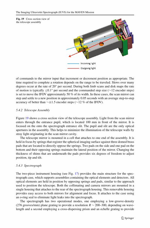
The Imaging Ultraviolet Spectrograph (IUVS) for the MAVEN Mission
Fig. 19 Cross section view ofthe telescope assembly
of commands to the mirror input that increment or decrement position as appropriate. Thetime required to complete a rotation depends on the range to be traveled. Slews over manydegrees occur at the rate of 20° per second. During both limb scans and disk maps the rateof motion is typically ≤0.1° per second and the commanded step size (∼12 encoder steps)is set to move the IFOV approximately 50 % of its width. In these cases, the scan mirror canstep and settle to a new position in approximately 0.05 seconds with an average step-to-stepaccuracy of better than ∼±1.5 encoder steps (∼12 % of the IFOV).
5.4.2 Telescope Assembly
Figure 19 shows a cross section view of the telescope assembly. Light from the scan mirrorenters through the entrance pupil, which is located 100 mm in front of the mirror. It isfocused on the onto the spectrograph entrance slit. The pupil and slit are the only opticalapertures in the assembly. This helps to minimize the illumination of the telescope walls bystray light originating in the scan mirror cavity.
The telescope mirror is mounted in a cell that attaches to one end of the assembly. It isheld in focus by springs that register the spherical imaging surface against three domed brasspads that are located to directly oppose the springs. Two pads on the side and one pad on thebottom and their opposing springs maintain the lateral position of the mirror. Changing thethickness of shims that are underneath the pads provides six degrees of freedom to adjustposition, tip and tilt.
5.4.3 Spectrograph
The two-piece instrument housing (see Fig. 17) provides the main structure for the spec-trograph case, which supports assemblies containing the optical elements and detectors. Alloptical elements are held in position by opposing springs and pads, similar to the approachused to position the telescope. Both the collimating and camera mirrors are mounted in asingle housing that attaches to the rear of the spectrograph housing. This removable housingprovides easy access to both mirrors for alignment and focus. It attaches to the case usingan o-ring seal to eliminate light leaks into the spectrograph.
The spectrograph has two operational modes, one employing a low-groove-density(276 grooves/mm) plane grating to provide a resolution R ∼ 200–300, depending on wave-length and a second employing a cross-dispersing prism and an echelle grating to provide

W.E. McClintock et al.
Fig. 20 The left panel shows the position of the grating flip mechanism (GFM) for the low-resolution mode.The GFM rotates the normal grating and its housing clockwise approximately 90° in order to illuminate thecross dispersing prism and echelle grating (right panel). When the GFM is positioned for echelle mode amask mounted on the side of the normal grating housing limits the height of the spectrograph entrance slit tobe 3 mm tall
R ∼ 12,500. A grating flip mechanism (GFM) rotates the normal-incidence grating and itshousing through an angle of 84.6° in order to switch between these two modes. The leftpanel of Fig. 20 shows the configuration of the GFM in the low-resolution mode. A steppermotor equipped with a planetary gear system that has a 49:1 ratio provides the rotationalmotion with a resolution of 0.037° per step. The motor is coupled to the bearing system thatsupports the normal-incidence housing through a torsionally compliant flexure. The GFMchanges modes by commanding the motor through 2303 steps in either direction to drive thegrating housing against two hard stops on the GFM body that are located ∼100 mm fromthe center of rotation of the grating and its housing. There is no position feedback in theGFM except for limit switches at either end of travel and registration against a hard stop isachieved by commanding a few extra steps to wind up the flexure so that it acts like a springthat forces the housing against the stop. Mechanical detents hold the housing in place oncepower is removed from the motor. Based on previous experience with this method of regis-tration, the repeatability for positioning the housing against the stop is ±0.025 mm, whichcorresponds to an angular reproducibility of ±0.25 milliradians (±0.014°). Therefore, acommand from low resolution to echelle and back again can cause a shift of up 0.25 mm inthe location of the spectrum at the detectors.
Figure 21 shows the detector module, which is a single housing that contains a beam split-ter, the detectors with their associated electronics, and a miniature mercury Penray® lamp,procured from UVP, an Analytik Jena Company. The entire module can be removed fromthe spectrograph structure as a unit, which facilitates assembly and optical alignment. Lightfrom the camera mirror first encounters the beam splitter, which contains 31 aluminizedrectangles that are 1.5 mm tall × 57 mm wide and that have a 2 mm center-to-center spac-ing (see Sect. 5.2.1). Approximately 57 % (75 % from the aluminized strips and 4 % from

The Imaging Ultraviolet Spectrograph (IUVS) for the MAVEN Mission
Fig. 21 The detector module includes a housing that supports a beam splitter, the FUV and MUV detectorassemblies and a mercury stimulus lamp. A high voltage power supply, not visible in the figure, is attachedto the bottom of the housing
the uncoated area) of the light incident on the beam splitter is reflected toward the FUVdetector. Light incident on the uncoated areas is transmitted to the MUV detector.
The FUV and MUV detector housings, which each contain a Hamamatsu V5180M imageintensifier and a fiber optic taper with 10 micron pore spacing that has a windowless CypressCYIH1SM1000AA-HHCS CMOS array bonded directly to its output surface. A compres-sion flexure registers the input surface of the taper against the output surface of the intensifierto maintain spatial resolution across the interface between intensifier phosphor and CMOSinput.
A 61 mm × 81 mm printed wiring board (PWB), which is soldered to the 84 pins of thej-lead ceramic chip carrier that encloses the CMOS array, provides both electrical connectionand mechanical support for the chip. The PWB is fastened to the fiber optic mounting bracketto form an integrated module, which is registered to the output of the intensifier with acopper-beryllium flexure. Six titanium struts are used to mount each detector housing to themodule. These provide six degrees of freedom for detector independent alignment and focusand serve to thermally isolate the detectors from the rest of the instrument.
Electrical connection to the CMOS arrays is made through a pair of ridged-flex circuitsto a single, 152 mm wide × 127 mm tall, detector-control board (DCB), which contains anRTAX2000 field programmable gate array (FPGA) that operates both detectors simultane-ously, performing all required binning/windowing and data compression. In addition to theFPGA, the DCB holds a pair of 2 M × 12 bit SRAM (one for each detector), which areused to perform double correlated sampling, and a pair of 1 M × 1 bit electrically erasableprogrammable read-only memory (EEPROM) that are used to store a bad pixel map foreach detector. After the RSDPU configures the detector FPGA by specifying the number ofimages, the imaging mode and windowing/binning configurations (Sect. 5.3), and the inte-gration time, the detector operates autonomously until the number of requested images withthe specified windowing/binning have been transmitted to a buffer in the RSDPU.
W.E. McClintock et al.
Once an imaging sequence is initiated by the RSDPU the DCB FPGA controls all sub-sequent timing and data transfer until the sequence is complete. Both single detector anddual detector operation are supported. Two serial low voltage differential signaling (LVDS)ports located on the DCB provide communications with the RSDPU. One operates asyn-chronously at 57.6 Kbits/sec for the command and configuration interface. The other op-erates synchronously at 5 Mbits/sec for data transfer to the RSDPU data buffer, which canhold up to seven full frame images from each detector.
A single image begins with a 1-msec detector reset, followed by a 230-msec-long readoutof a black level image, which is stored in one side of the 2 M × 12 SRAM. Next, the detectorFPGA issues an ‘open shutter’ command to the RSDPU. At the end of the integration timethe detector FPGA reads out the array replacing each stored black level value in the SRAMwith the just-read value minus the stored black level. If both FUV and MUV images havebeen requested by the RSDPU, these steps occur simultaneously in the two detectors. Whiledata are read into the first side of SRAM, the previously recorded image is transferred to theRSDPU data buffer from the second side of SRAM. Removal of bad pixels, windowing andbinning, and data compression are performed on the fly during the transfer using 16-bit widewords. Although the detector FPGA initiates a shutter open command for the two detectorssimultaneously, the RSDPU controls the ‘shutter close’ timing independently for each. Thisenables different FUV and MUV integration times. The CMOS detector output is digitizedto 12 bits. If more that 16 pixels are co-added while forming a binned word for transmissionthere is a potential for overflow. This is addressed by using a 26-bit wide summing register.After summation the 26 bits are reduced to 16 using a pseudo-logarithmic algorithm inwhich the 12 bits following the first ‘1’ in the summed value are used as the mantissa andthe exponent is ones-complement of the 4 bit representation of the number of leading ‘0’s inthe summed value.
A HVPS designed by Battel Engineering, is attached to the bottom of the detector mod-ule, and provides the voltages required to operate the FUV and MUV image intensifiersindependently. These include fixed −6000 V biases for the phosphors (relative to their re-spective MCP output voltages) and variable voltages in the range 200–1000 V for the MCPinput voltage. The HVPS also applies one of two fixed voltages between the intensifier pho-tocathode, which is located on the inside of the intensifier input window, and the input of theMCP providing an electronic shutter. When the photocathode is held at +40 V relative tothe MCP photoelectrons are accelerated into it producing a cascades of electrons. When thephotocathode is held at −200 V relative to the MCP no acceleration occurs and no cascadesoccur.
A low-pressure cold cathode mercury gas lamp, produced by Penray®, is attached to thetop of the beam splitter housing. Its principal ultraviolet emissions are two atomic lines thatare located at 184.9 nm and 253.7 nm. These are isolated for the FUV and MUV detectors,respectively, using passband filters made by Princeton Instruments. The lamp is used forend-to-end (detector-instrument-spacecraft-ground system) testing when it is not practicalto use the instrument optical system. It is also used for tracking any spectral ‘imprinting’that may take place during operations around Mars.
5.5 Thermal Subsystem
The CMOS arrays in the IUVS detectors operate at temperatures near −20° in order tominimize the effects of dark current noise in the IUVS data (see Fig. 21). This is accom-modated by the thermal subsystem using two temperature zones because maintaining theentire instrument at these temperatures using passive techniques requires an unrealistically

The Imaging Ultraviolet Spectrograph (IUVS) for the MAVEN Mission
Fig. 22 Predicted performance of the thermal subsystem
large radiator. Using a second thermal zone that is maintained near room temperature forthe optics and structure also simplifies alignment, focus, and optical testing. A third thermalzone was implemented for RSDPU thermal control because it can tolerate a wider range oftemperature and is physically isolated from IUVS.
IUVS and the RSDPU are thermally isolated from the APP using titanium struts and G10fiberglass spacers, respectively to achieve a power transfer across the mechanical interfacesto <0.05 W/°C for each component. Titanium mounting flexures were also used to reducethe conduction between the telescope baffles and the instrument housing to <0.05 W/°C.Both IUVS and RSDPU are entirely enclosed in thermal blankets except for the input aper-tures of the IUVS baffles.
The thermal subsystem uses radiators attached to the instrument case, detector housing,and RSDPU housing to reduce the temperatures to less than the desired minimum operatingvalues. A single radiator attached to the top of the detector housing cools a pair of units(FUV and MUV) each containing an intensifier, fiber taper, CMOS array, and read electron-ics. The telescope apertures provide radiators for the telescope and scan mirror assemblies.In addition three small radiators are attached to the top of the spectrograph housing at thefront, middle and back. A radiator is attached to the top of the RSDPU housing. The RSDPUmonitors the temperatures of the three zones and controls them by turning on and off oper-ational heaters to maintain values within high and low limits that are uploaded by groundcommand.
Thermal models were used to determine radiator and heater sizes and placements. Heatloads into the instrument and radiator view factors were obtained from detailed spacecraftmodels for the entire mission and include orbital geometry, spacecraft attitude, and APPorientation. The goals for the design were to maintain detector temperatures at 0 °C orlower in order to control dark current and to minimize diurnal temperature variations in thespectrograph in order to minimize wavelength shifts caused by changing thermal gradientswithin the case. Figure 22 summarizes the predicted performance of the thermal subsystemover the nominal mission life. Temperature ranges shown in Fig. 22 include both diurnal andseasonal variations. For IUVS diurnal thermal variations dominate seasonal variations butthese are still less than ±3° for all components. Detector temperatures are expected to range

W.E. McClintock et al.
between −25°C and −20 °C. This will limit the dark current to 0.25 DN/sec. For RSDPUthe magnitude of the seasonal variations is ∼35 °C with additional ±5 °C diurnal variations.This is acceptable because the RDSPU contains no mechanisms or optical components andthe resulting range is well within the operating specifications for the electronic parts.
5.6 Data Processing Unit
The RSDPU is the electrical interface between the IUVS and spacecraft and provides thepower and drivers required to operate the IUVS detectors and mechanisms. It is enclosed ina 25.0 × 32.0 × 9.9 cm3 aluminum box that is attached APP interface plate on the oppositeside from the IUVS. The RSDPU contains a pair of PWBs referred to as the power boardand processor board, respectively.
The processor board is built around an RTAX2000 FPGA that contains an embedded8051 microcontroller core (Core8051) supplied by Actel Corporation. In addition to pro-viding the command and data interface to the spacecraft, which operates asynchronously at57.6 Kbps over an RS-422 serial link, the FPGA controls all of the subsystems within theIUVS. These include:
• Independent command and control of each detector high voltage power supply (HVPS)for, HVPS power on/off, intensifier phosphor voltage on/off, high voltage level for theMCPs, and photocathode shutter open/close
• Actuation of the grating flip mechanism• Operation of the detector stimulus lamp• Operation of the scan mirror including the implementation of the PID algorithm used to
position the mirror• Control of the instrument’s heaters• Collection of housekeeping data including various voltages, temperatures, and configura-
tion monitors (e.g. grating flip position)• Configuration of image windowing and binning• Storage of images, including a ping pong buffer capable of storing up to 14 full frame
images from each detector.
The processor board also supports two 128 K × 8 SRAMS for storage and executionof system code and for microprocessor data memory as well as a 128 K × 8 EEPROM fornon-volatile storage of program code. This enables the RSDPU to execute both immediatecommands received over the spacecraft interface and stored sequences of commands.
The RSDPU power board contains a low voltage power supply that converts +28-voltspacecraft power to the various voltages required to operate the IUVS subassemblies. Theseinclude ±15 v, +5 v, +5.6 v, +3.9 v, and +2.2 v. All subassemblies receive power directlyfrom the power board, which also transmits control signals from the processor board to theHVPS for setting MCP high voltage and adjusts the current flow through the scan mirrorLED. These functions are enabled by digital to analog converters (DACs) on the powerboard. The power board also houses the drive circuits for the scan mirror and grating flipmotors, switches for spacecraft power to the heaters, the analog-to-digital converter (ADC)used to sample and digitize sine and cosine voltages from the scan mirror encoder, instru-ment housekeeping voltages, and temperatures.
6 Measurement Performance
During instrument design we used models to predict its measurement performance, includ-ing imaging, spectral resolution, and radiometric sensitivity. These were based on raytrace

The Imaging Ultraviolet Spectrograph (IUVS) for the MAVEN Mission
analysis, measurement of component performance at LASP (detector imaging, dark current,read noise, intensifier gain and photocathode quantum efficiency) and vendor specifications(grating efficiency, mirror reflectivity, and beam splitter transmission). The performancecharacteristics of the instrument, including radiometric sensitivity, were also measured bothbefore and after instrument environmental test and qualification. Any important differencesbetween modeled and measured performance are noted below.
6.1 Conversion of Instrument Data Numbers to Geophysical Units
IUVS measures the radiance arriving at the entrance pupil of the instrument from the Marsatmosphere, and Eq. (11) defines the conversion of instrument output (data numbers) togeophysical data (radiance or reflectance):
L(λj , θk) = [DN(λj , θk) · N(DN(λj , θk)) − DNDark(λj , θk) − Sl(λj , θk)]/�t
A · �λ · Ω(θk) · R(λj , θk)(11)
Here DN is the detector data number output for signal accumulated during integrationtime �t in a single pixel with index j, k associated with wavelength (λj ) and angularposition along the spectrograph entrance slit (θk). N is the detector linearity correction.DNDark is the pixel data number resulting from dark charge collected during �t . A is thearea of the entrance pupil, �λ is the spectral passband of the spectrograph for a singlepixel, and R is the instrument responsivity for pixel j, k. Sl is a stray plus scattered lightcorrection (Sl = S ′
l + SStray). Sl is positive for bright spectral features (more light is scat-tered out of pixel j, k than is scattered in by all other wavelengths), and negative for faintspectral features (less light is scattered out of pixel j, k than is scattered in from all otherwavelengths). SStray represents the light that is diffusely scattered from internal instrumentsurfaces. Ω(θk) = w(θk) · hpix · F−2
Tel is the solid angle subtended by an aperture definedby the height of a pixel and the width of the spectrograph entrance slit for position θk .R = TOptics ·QePc ·GDet ·GADC is the product of the optics transmission, detector photocath-ode efficiency, and the detector gain stages.
Detector dark current will be measured by periodically closing the detector electronicshutter throughout each orbit. Nonlinearity is caused by well saturation in the CMOS de-tectors and by differential nonlinearity in the analog-to-digital converter. It was charac-terized during detector calibrations before launch. The scattered light correction also ap-pears in the numerator as a value that must be subtracted from observed signal to cor-rect for light scattered from all other wavelengths into position/pixel j, k: S ′
l (λj , θk) =A · �λ · Ω(θk) · ∫
L(λ′) · R(λ′, θk) · G(λj − λ′)dλ′, where G is the grating scatter distri-bution function (GSDF), which is often approximated as a Lorentzian profile plus constantbackground (Woods et al. 1994). Pre-launch values for the various parameters appearing inEq. (11) were determined during instrument characterization and calibration using both ra-diance and source standards. Radiometric calibrations using radiance standards (irradiancestandards and reflectance screens) that fill the instrument aperture and FOV measure thequantity A · �λ · R(λj , θk) · Ω(θk). Calibrations using standard detectors and star sourcesthat fill only the aperture measure A ·R(λj , θk), and Ω(λj ) and �λ must be determined sep-arately by scanning the FOV and measuring monochromatic lines, respectively. After launchobservations of stars during cruise provide measurements of A · R(λj , θk) · �λ that will beaccurate to ∼10 % (Snow et al. 2013). No specific requirements were placed on SStray, whichis bookkept in the constant term of the GSDF and was not independently characterized be-fore instrument assembly. Instead, the sum of the constant term plus SStray was determined

W.E. McClintock et al.
during instrument calibration. This was accomplished for the FUV channel during vacuumtesting by measuring the residual signal at wavelengths less than the short wavelength cutoffit MgF2 window (<115 nm) and for the MUV channel during ambient testing by measuringthe residual signal at wavelengths less than the air cutoff (<180 nm).
6.2 Characterization and Preliminary Calibration Results
6.2.1 As-built Optical Configuration
There were two significant modifications to the IUVS optical configuration during develop-ment. The first occurred late in the development when we discovered that the ruling densityof the delivered normal incidence gratings from the manufacturer was 286 lines mm−1 in-stead of the 276 lines mm−1 that was specified in the purchase order. This led to ∼4 %increase in dispersion that has no significant impact on performance.
The second occurred early in the development when we discovered that approximately5 % of the zero order beam from the normal incidence grating impinged upon the collimatormirror. If the initial design were retained the collimator would focus this light back onto thegrating to form an image of the entrance slit. The grating would then diffract the light fromthis image toward the camera mirror, which would project an out-of-focus a secondary spec-trum onto the detectors. This problem was solved by increasing the normal grating openingangle and repositioning the camera mirror. While this approach had a negligible impact onnormal incidence mode performance, it significantly altered the efficiency function of theechelle (Eq. (5)), shifting deuterium Lyman alpha away from the blaze peak. The measuredas-built opening angle to the center of the FUV detector for the echelle was 13.32°, placing121.37 nm at the blaze peak and reducing strength of the deuterium Lyman alpha emissionto 0.65 relative to the blaze peak. Because the free spectral range of the echelle spectrum is<12 mm (Sect. 5.2.1) the loss in sensitivity was partially mitigated by reducing the echelleopening angle to 12.74° so that the echelle pattern to covers only one half of the FUV de-tector. In this configuration the strength of the deuterium emission relative to blaze peak isincreased to 0.85.
6.2.2 Detector Characteristics
Intensifier Gain Equation (11) describes the relationship between L(λj , θk), the radianceat the IUVS entrance pupil, and DN(λj , θk), the data numbers readout from the detectorafter an integration time �t . DN(λj , θk) is directly proportional to the gain of the MCP inthe image intensifier (Eqs. (6)–(8)), which can be adjusted by varying the voltage appliedacross the MCP input and output surfaces. Typical gain values for the MCPs in the IUVSintensifiers (Hamamatsu V5180M) range between 1 and 1000 for voltages between 500 and900 volts.
Relative gains for the flight intensifier MCPs were measured over the 400–650 volt rangebefore the intensifiers were installed in the instrument. After installation the gains were char-acterized by comparing the response to spectral lines of different strengths while varying theintegration time and voltage. This allowed us to measure the entire 400–900 volt range. Fig-ure 23 shows the relative voltage-gain curves for both MUV and FUV obtained from thosecalibrations. We were only able to determine the relative gain because no independent mea-surements were made for the rest of the detector components, which include photocathodequantum efficiency, phosphor gain, fiber-optic taper transmission, and HAS detector quan-tum efficiency (Eqs. (6)–(8)). The results shown in Fig. 23 have been normalized so that

The Imaging Ultraviolet Spectrograph (IUVS) for the MAVEN Mission
Fig. 23 Relative intensifier MCPgain as function of appliedvoltage. The two curves havebeen normalized to G = 1000 forV = 900 volts
GMCP = 1000 for V = 900 volts in order to be consistent with nominal values published inthe Hamahatsu image intensifier catalog.
In addition to measuring the MCP relative gain, we calculated the product of GDet ∗GADC ,which is the number of output DNs per photoelectron produced by the photocathode, fromestimated values of the remaining parameters in Eqs. (6)–(8) using published values from thecomponent manufacturers. These are phosphor gain (GPhos = 70) from Hamamatsu, CMOSdetector quantum efficiency (0.45) and ADC gain (25 e−/DN) from the HAS specificationdata sheet. For the fiber-optic transmission we assumed that it has a bulk transmission (in-cluding reflection losses at the input and output) of 0.8 and that the numerical aperture is0.4, resulting in a transmission of 0.32. Inserting these values into Eq. (8), gives an over-all detector maximum gain (V = 900 volts) at the CMOS output that is ∼104 e− for eachphotoelectron produced by the photocathode. This is ∼400 DN at the ADC output for eachphotoevent.
CMOS Characteristics The CMOS detectors operate in correlated double sampling/ non-destructive read mode CDS/NDR (Sect. 5.3), which eliminates fixed pattern offsets, reset(kTC) noise, and lag at the expense of increasing the readout noise by
√2. In this con-
figuration only dark current noise and readout noise persist. These were measured over abroad temperature range (−40 °C to +20 °C) during unit-level testing. Both detectors havenearly identical mean thermal response described by DN = 1.29 ∗ tint ∗ exp0.088T where DNis the average dark signal data number accumulated during integration time tint and T is thetemperature in °C. Dark signal noise is the square root of the number of signal electronscollected during an integration period converted to DN. For the IUVS detectors the gain is0.04 DN per electron (Sect. 5.3) and the σ(DN) = √
tint ∗ 0.23 exp0.044T . Read noise, whichis essentially independent of temperature, is 2.9 DN for CDS/NDR.
The IUVS thermal subsystem is designed to maintain CMOS detector temperatures be-low −20 °C throughout the orbital mission. At these temperatures the average dark signalrate is 0.22 DNsec−1 per pixel and typical dark signals vary from 0.44 DN per pixel forlimb altitude profiles where the integration period is 2 sec to 13.3 DN per pixel for apoap-sis images where the integration period is 60 sec. Dark signal noise values for these twointegration periods are 0.13 DN and 0.74 DN, respectively.
Full well depth for the IUVS detectors is ∼105 electrons corresponding to a typical am-plitude of 1.5 volts on the column amplifiers. When the number of electrons accumulatedin an individual pixel is less than 8 × 10⁴, the output gain is 15 µV per electron (0.04 DNper electron). Above this level the output gain rapidly declines; therefore IUVS intensifier
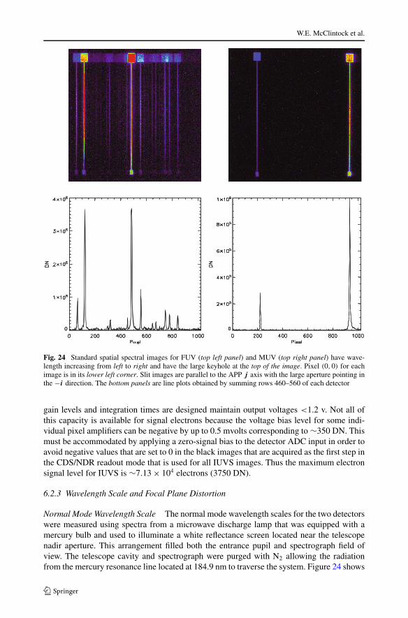
W.E. McClintock et al.
Fig. 24 Standard spatial spectral images for FUV (top left panel) and MUV (top right panel) have wave-length increasing from left to right and have the large keyhole at the top of the image. Pixel (0,0) for eachimage is in its lower left corner. Slit images are parallel to the APP j axis with the large aperture pointing inthe −i direction. The bottom panels are line plots obtained by summing rows 460–560 of each detector
gain levels and integration times are designed maintain output voltages <1.2 v. Not all ofthis capacity is available for signal electrons because the voltage bias level for some indi-vidual pixel amplifiers can be negative by up to 0.5 mvolts corresponding to ∼350 DN. Thismust be accommodated by applying a zero-signal bias to the detector ADC input in order toavoid negative values that are set to 0 in the black images that are acquired as the first step inthe CDS/NDR readout mode that is used for all IUVS images. Thus the maximum electronsignal level for IUVS is ∼7.13 × 10⁴ electrons (3750 DN).
6.2.3 Wavelength Scale and Focal Plane Distortion
Normal Mode Wavelength Scale The normal mode wavelength scales for the two detectorswere measured using spectra from a microwave discharge lamp that was equipped with amercury bulb and used to illuminate a white reflectance screen located near the telescopenadir aperture. This arrangement filled both the entrance pupil and spectrograph field ofview. The telescope cavity and spectrograph were purged with N2 allowing the radiationfrom the mercury resonance line located at 184.9 nm to traverse the system. Figure 24 shows

The Imaging Ultraviolet Spectrograph (IUVS) for the MAVEN Mission
Fig. 25 Echelle image of an N + N2 emission spectrum obtained during instrument calibration using alamp that only fills 1 mm of the 3-mm-tall echelle entrance slit. The left panel is the raw FUV image. Atomicemission features appear in the lower 60 % of the image. Emissions from the Lyman-Birge-Hopfield system ofN2 dominate the upper 20 % of the image. The brightest emissions arise from NI 124.318 nm and 124.331 nmfollowed by NI 119.955, 120.022, 120.720 nm. The right panel is a model of IUVS echelle mode for atomic N
an example of images obtained from this experiment. The upper left and right panels are rawimages from the MUV and FUV detectors, respectively, recorded using CDS/NDR. Lowerpanels show line plots obtained by summing rows 460–560 of the detector images.
The wavelength scale for column N of the detector, λ(N), is determined from Eq. (1)with α fixed and β calculated from Eq. (12) with � ∼ 0.0234 mm and with βc ∼ 8.8° forFUV detector and βc ∼ 8.0° for the MUV detector, respectively,
βN = βc + tan−1((N − 511.5) · �/F
). (12)
In practice λ(N) can be adequately approximated by a simple quadratic,
λ = λ0 + aλ · N + bλ · N2, (13)
which reproduces the solution to Eqs. (1) and (12) to better than ±0.02 · aλ.Gaussians were fit to the isolated lines in the plots in the lower left panel of Fig. 24
for MUV and the central-wavelength parameters from those fits were used as estimates ofline centers. These were fit to Eq. (13) using a standard least squares algorithm resultingin l0 = 174.63, a1 = 0.16215, and b1 = 2.4201 × 10⁻⁶. These values provide in a nominalspectral coverage and dispersion for the central 100 rows of the images shown in Fig. 24 of174.6–343.0 nm with an average 0.1646 nm per pixel (7.017 nm/mm) spacing. The sameapproach was used for FUV except only two lines are available (253.6 nm in 1st order and184.9 nm in 2nd order) so only the coverage, 109–192 nm, and average spacing of 0.0814 nmper pixel (3.47 nm/mm) are determined from these data. Inserting the dispersion values intoEq. (3) yields a value for the grating spacing, d−1 = 286.0 g/mm with f = 495.1 mm. Thisgroove spacing is significantly different from the d−1 = 276.0 g/mm specific in the purchaseorder to Jobin Yvon. The origin of this discrepancy has not been identified.
Echelle Mode Wavelength Scale The IUVS employs the combination of a short entranceslit (3 mm tall in echelle mode compared to 22 mm tall in normal mode, Sect. 5.4.3) and

W.E. McClintock et al.
a MgF2 cross disperser prism, located directly in front of the grating, to spatially separatesoverlapping grating orders. The result is a two dimensional spectral image or echellegram.The left panel in Fig. 25 shows an example of an echellegram of N + N2 obtained duringground calibration using a lamp that filled only 1 mm of the 3 mm tall slit. The spectrumconsists of isolated atomic features over approximately 70 % of the wavelength range. Emis-sions from the Lyman-Birge-Hopfield system are evident for wavelengths greater ∼123 nm.The pattern is shifted left by ∼250 pixels relative to the simulation shown in Fig. 15 toaccount for an adjustment to spectrograph geometry, which was made during instrumentdesign and fabrication (see Sect. 6.2.1). The right panel is a model of the echelle mode foratomic N, which uses a line list from the NIST atomic database, that predicts the location ofthe brightest features in the echelle spectrum using the grating equation and the dispersionrelation for the MgF2 prism (Sect. 5.2.3).
In contrast to normal mode, the echelle mode wavelength scale cannot be represented bya simple polynomial. Instead, the wavelength associated with each pixel must be specifiedusing the prism equation for its row number and the grating equation for its column. For athin prism with apex angle A, the difference in deviation angle for light with wavelength λ
and wavelength λ0 traversing the prism is related to the index of refraction by the equation�θ = A ·(n(λ)−n(λ0)). In IUVS the echelle grating is tipped so that light from the center ofthe entrance slit with wavelength λ0 = 121.5 nm impinges upon it with γ = 0 (Eq. (1)). Thisbeam is diffracted by the echelle and emerges undeviated in the cross-dispersion dimensionafter a second pass through the prism. All other wavelengths impinge upon the echelle atangles γc = �θ and deviated by 2γc = 2�θ after traversing the prism twice. The numberfor each row of the detector is related to wavelength λ by
2 · γc = tan−1((N − 511.5) · �/F
)(14)
γc = A · (n(λ) − n(λ0))
(15)
Similar to the normal mode, the grating equation relates wavelength to column positionthrough Eqs. (1) and (12). These results relate detector position to wavelength for lightoriginating from the spectrograph slit center. For heights, h, above and below the slit
2 · γ − h/F = tan−1((N − 511.5) · �/F
)(16)
γ = A · (n(λ) − n(λ0)) + h/F (17)
where −1.5 mm ≤ h ≤ 1.5 mm.
Focal Plane Distortion The fiber optic couplers in the two detectors that connect the outputof the intensifiers to the CMOS arrays are fabricated from thick (approximately 20 mm long)faceplates that are drawn to form tapers. This process introduces distortion in the faceplatesand the 24 mm square focal planes at their inputs map to trapezoids at their outputs. Thus,each row of the CMOS arrays has a different wavelength scale.
We used images shown in Fig. 24 to measure distortion by fitting Gaussians to the emis-sion lines in 8 individual spectra made by summing 100 rows at a time beginning with rows200 ± 50 and ending with rows 900 ± 50. The results indicate that the distortion is not uni-form. For the MUV detector, slit images at the longest wavelengths are twisted clockwiseby 3 pixels while those at the shortest wavelengths are twisted counter clockwise by 1 pixel.For the FUV detector, slit images at the longest wavelengths are twisted counterclockwiseby 2 pixels while those at the shortest wavelengths are aligned with the detector column.Thus, using the wavelength scale derived from the central rows of the detector can lead to

The Imaging Ultraviolet Spectrograph (IUVS) for the MAVEN Mission
errors of up to 1 pixel at the top and bottom of the MUV detector and slightly less than 1pixel for the FUV detector. Focal plane distortion has only a small effect on echelle modebecause slit images for individual spectral features are ∼3 mm tall.
The values of λ0 determined for the images in Fig. 24 are 108.91 nm and 174.56 nmfor FUV and MUV, respectively. These values can change by up to ∼±0.8 nm for FUVand ∼±1.6 nm for MUV after a GFM cycle has moved the normal incidence grating out ofand back into the collimator beam (Sect. 5.4.3). It is possible that the magnitudes of thesedisplacements will decrease with repeated actuation of the GFM during orbit.
6.2.4 Line Spread Function and Spectroscopic Resolution
Normal Mode The top panel in Fig. 26 shows a 41 × 41 pixel window from an imageof the system PSF near the center of the detector field of view, which was obtained usinga collimator equipped with a scanning grating monochromator to produce a simulated starsource with an angular size 0f 0.2 mrad at a single isolated wavelength. Although its core isrotationally symmetric, the image displays wings that extend along both the dispersion andcross-dispersion axes.
The black curve in the bottom panel shows the line spread function (LSF) in the disper-sion direction, which was constructed from the sum of all the rows in the top panel image.Red and blue curves show the best-fit Gaussian and Voigt (the convolution of a Gaussianand a Lorentzian function) profiles, respectively. Whereas the FWHM derived for both fitsis approximately 6 pixels, the Voigt functional form is clearly required to fit the far wings ofthe PSF.
Although the exact origin of the PSF wings is uncertain, several factors are likely to con-tribute to them. In the cross dispersion direction the beam splitter acts as a coarse grating.The beam splitter pattern is 2 mm tall (1.5 mm reflective and 0.5 mm transmissive) andlight from the camera mirror illuminates approximately 10 cycles of this pattern as it ap-proaches the focal plane. The resulting diffraction/interference pattern has an envelop that iswell approximated by a Gaussian function with FWHM ∼0.06 mm for MUV and FWHM∼0.01 mm for FUV, respectively. This effect is not large enough to account for the mea-sured profile. Rough grating grooves and ordinary grating scatter can also lead to broadwings on the grating distribution function, which would affect the PSF in the dispersiondirection. This usually results in light scattering over large angles, which is not the effectobserved here. Mid-frequency wave-front errors (MFWFE) introduced by zonal polishingof the toroidal camera mirror can also contribute. Finally, some researchers have reported‘halos’ around point-source images obtained with intensified CMOS detectors (Ren et al.2014) Unlike the ‘+’ pattern observed here, both MFWFEs and detector halos are rotation-ally symmetric.
We adopted the FWHM of the emission lines shown in the top panels of Fig. 24 as themeasure of the instrument spectral resolution for an extended source that covers the en-tire spectrograph entrance slit width. Figure 27 summarizes the performance using FWHMvalues determined from the 8 equally spaced spectra in the distortion analysis. When com-bined with the dispersion, these results indicate that the MUV spectral resolution varies from∼0.82 nm to ∼1.11 nm (MUV uses the left 24 mm of the focal plane) across the focal plane.The FUV spectral resolution varies from ∼0.42 nm to ∼0.63 nm.
These are slightly larger than predicted by the optical model (Fig. 12) with a maximumvalue of 0.18 mm here compared to 0.16 mm for the model. Figure 27 also reveals that themorphology of the FWHM contours in the as-built instrument, which shows a minimumnear the center of the bottom row, differs significantly from that of the model, which shows

W.E. McClintock et al.
Fig. 26 The top panel is a41-pixel square image of theimaging point spread function(PSF). The black curve in thebottom panel is the line spreadfunction (LSF), which wasconstructed by summing all therows of the image in the toppanel. Red and blue curves arebest-fit profiles using a Gaussianfunction (red) and a Voigtfunction (blue)
contours that are nearly uniform in dispersion and increase both above and below the centralrow. It is possible that the asymmetry observed here is a result of distortion introduced byone or both of the three-point mounts holding the collimator and camera mirrors.
Echelle Mode We estimated the echelle mode line spread function in the dispersion di-rection for a filled entrance slit using a line plot extracted from the image shown in the leftpanel of Fig. 25. The left panel of Fig. 28 shows the spectral plot for orders 350 and 351,which was obtained by summing rows 300 through 400 of the image in Fig. 25. There isclear evidence for a broad continuous background that peaks near pixel 250 (see also the

The Imaging Ultraviolet Spectrograph (IUVS) for the MAVEN Mission
Fig. 27 The imaging pointspread function for thespectrograph when the entranceslit is uniformly illuminated.When combined with the systemdispersion the resulting spectralresolution varies across the focalplane from ∼0.82 nm to∼1.11 nm for MUV and from∼0.42 nm to ∼0.63 nm for FUV
Fig. 28 The left panel is a line plot of orders 350 and 351 produced by summing rows 300–400 of the imagein the left panel of Fig. 25. The right plot shows Gaussian (green) and Voigt (blue) fits to the profile centerednear pixel 650
image in the left panel of Fig. 23). This is most likely due to grating scattered light, which ismuch stronger for echelles than for typical normal incidence gratings (Content et al. 1996).Gaussian (green) and Voigt (blue) fits to the profile center near pixel 650 are shown in theright panel of Fig. 28. These results show that a Voigt profile more accurately represents theprofile than a Gaussian, which is consistent with the normal mode profile.
Whereas the FWHM of the normal mode profile in the as built instrument is comparableto the FWHM obtained from ray trace modeling (paragraph “Normal Mode WavelengthScale”), the FWHM of the echelle profile is 50 % larger than that of the model profileprediction. The source of this discrepancy is not understood. Referring to Eq. (4), the lineardispersion at hydrogen Lyman alpha (121.567 nm) is 0.0309 nm/mm (n = 346 and β =76.25◦) and spectral resolution for the measured profile is �λ = 9.43 × 10⁻³ nm (�w =13 pixels = 0.305 mm) or R = λ/�λ = 12,900. This compares to 19,000 inferred from theraytrace model.
The deuterium Lyman alpha line center, at 121.534 nm, is displaced by 0.033 nm(1.07 mm = 45.6 pixels) relative to its hydrogen counterpart and is therefore well resolved,even at R = 12,000. On the other hand, the intensity in wings of the hydrogen emission

W.E. McClintock et al.
line 45 pixels from line center is approximately 1 % of the peak emission and this is likelythe limiting factor for detecting weak D emission from the Mars atmosphere. (Note thatthe additional background present in the profile shown in the right panel of Fig. 28 arisesfrom scattering of the three bright emissions in order 350.) A similar background should notbe present in the Mars data because H dominates all other emissions by a factor of 100 orgreater. Thus background observed at the D line wavelength is expected to arise from thenearby H line only and is expected to show a level approximately equal to 1 % of the peakof the H line.
6.2.5 Radiometric Sensitivity
Normal Mode IUVS normal-mode radiometric sensitivity was measured using both detec-tor standards (comparison of instrument response to that from a calibrated photodiode) andirradiance standards (calibrated lamps). Both approaches are traceable to National Instituteof Standards and Technology (NIST) standards.
In the former calibration approach we used a vacuum facility equipped with a 2.3-m-focal-length collimator that had a scanning monochromator positioned at its focal plane. Themonochromator’s exit slit was masked to 1 mm in height and the slit was adjusted to be lessthan 0.2 mm wide so that beam of light exiting the collimator had less than a 0.2 milliradianangular extent. A hollow cathode lamp using flowing H2, N2, O2, and CO2 was placed at theentrance slit provided spectra with both molecular emissions and isolated atomic emissions.A pair of photomultiplier tubes (PMTs) with pulse-amplifier-discriminators and 2.54-mm-square apertures were placed on a translation stage in the vacuum chamber and coaligned tothe IUVS. One of these was equipped with a CsI photocathode and a MgF2 window for FUVcalibrations and the other with a CsTe photocathode and a fused silica window for MUVcalibrations. The PMTs’ quantum efficiencies were determined as a function of wavelengthby comparing their outputs to a photodiode whose absolute quantum efficiency as a functionof wavelength was measured by NIST (Canfield et al. 1973). This allowed us to determinea map of input beam irradiance (photons cm−2 sec−1) as a function of position within thevacuum chamber by scanning the two PMTs in a raster pattern and measuring their outputs.IUVS responsivity, R(λj , θk) (R = TOptics ·QePc ·GDet ·GADC) was determined at 20 discretewavelengths and 7 heights along the slit. A measurement sequence for each wavelength andangle began setting the monochromator to an isolated atomic emission line and mapping thebeam with the appropriate PMT. Once map was complete, the PMT was placed in the centerof the raster and its count rate was recorded. Next the PMT was translated aside and theIUVS placed at the center of the raster and rotated in elevation to the measurement angle,θk , where the DN rate was measured. Finally the PMT was reinserted and its count rate wasmeasured for a second time to determine lamp drift. (No more than a few percent drift wasever observed during a measurement sequence). Two separate measurement sequences wereperformed; one with the monochromator grating grooves parallel to those of IUVS and onewith them perpendicular. These were averaged to account for polarization effects that mayhave been introduced because the monochromator grating acts as a polarizer and the IUVSgrating acts as an analyzer. (The effects were only a few percent, probably because the IUVSgrating operates very near the Littrow configuration (James & Sternberg 1969).) Care wastaken to accurately account for parallax between the PMTs whose apertures were in oneplane and the IUVS whose entrance pupil was in another.
The irradiance standards approach is performed at ambient pressure and can onlybe used for MUV. It employs lamps that have their spectral irradiance (i.e., photonscm−2 sec−1 nm−1) directly traceable to NIST standard sources. In this approach a calibrated

The Imaging Ultraviolet Spectrograph (IUVS) for the MAVEN Mission
Fig. 29 Responsivity curves forFUV and MUV channelsmeasured before launch. Thesecurves represent the efficiency ofthe optial-detector system. Thesignal produced by IUVS foratmosphere emission is theresponsivity multiplied by theetendue of the optical system
lamp (irradiance standard) is placed in front of a Spectrolon® screen providing an extendedsource with a radiance (i.e., photons cm−2 sec−1 nm−1 str−1). Radiance is calculated fromthe product of lamp irradiance at the screen multiplied by screen reflectance (Georgiev andButler 2007; Stiegman et al. 1993). When IUVS views a screen that is large enough to fillboth its entrance pupil and its field of view the output DN rate from the MUV detector di-vided by the screen radiance is a direct measure of the quantity A · �λ · R(λj , θk) · Ω(θk).A measurement sequence includes observations of the screen followed by a dark measure-ment, obtained by closing the MUV electronic shutter. This is followed by a similar sequencewith the screen by a black cloth. Assuming that the cloth reflectance is ≤4 % provides agood measure of the ambient backgrounds, which result when light from the lamp is re-flected from walls and other objects within the lab into the IUVS field of view. Additionally,measurements are made at a range of instrument-screen separations in order to determine at-mospheric absorption, which is small but significant, particularly for wavelengths <240 nm.Both a deuterium lamp (Saunders et al. 1978), which was calibrated for λ > 200 nm, andan FEL lamp (Walker et al. 1987), which was calibrated for λ > 250 nm, were used forIUVS. The different spectral properties of these lamps provide insight into the scatteredlight performance of the IUVS spectrograph.
Figure 29 is a plot of the composite responsivity at FOV center obtained by combiningthe results from the vacuum calibration (FUV and MUV) with those from the two lamps(MUV only). These are plotted for the respective maximum MCP gains (900 v). We esti-mate the overall uncertainty in responsivity curves to be ∼20 % for FUV and ∼15 % forMUV. These estimates will be refined during cruise to Mars using observations of brightultraviolet-emitting stars, whose irradiances known to 10 % or better (Snow et al. 2013).A detailed analysis of the ground calibration results and their uncertainties and a compari-son with cruise measurements will discussed in a subsequent paper.
Photon arrival is a random process described by Poisson statistics. When Nphot are thenumber of signal photons detected during a single integration period, the estimate for theuncertainty in the mean value of Nphot for many integration periods, which is often referredto as noise, is
√Nphot. When an image intensifier is employed in the instrument then the
uncertainty is√
(E ∗ Nphot) where E is the intensifier excess noise (Sect. 5.3). The respon-sivity reported here is the product, NDN = Nphot ∗ GDet ∗ GADC; therefore, the uncertainty is√
NDN ∗ √(E ∗ GDet ∗ GADC).
During detector calibration we estimated GDet ∗ GADC . This was accomplished by illu-minating the detector so that only a few thousand photon events were collected during an

W.E. McClintock et al.
integration, determining the centroids of individual events in the output images, and inte-grating the DNs for the pixels within a 4 × 4 pixel box centered on the centroid. The resultsare GDet ∗ GADC = 390 DN/phot for MUV and GDet ∗ GADC = 460 DN/phot, both for anMCP voltage of 900 v. (For example, noise = 30 ∗ √
NDN and 28 ∗ √NDN for FUV and
MUV, respectively, when MCP voltage = 900 v.) These values will also be refined in flightusing stars.
The signal produced by IUVS for atmosphere emission is the responsivity multipliedby the etendue of the optical system. For example the etendue for a normal-mode obser-vation that includes the entire length of the airglow slit (0.1 mm wide × 19.8 mm tall) isAS ∗ AT /F 2
T = 0.01 ∗ 1.98 ∗ 1.33 ∗ 2/100 = 5.28 × 10⁻⁴ cm2 steradian, where AS and AT
are the slit and telescope areas and FT is the telescope focal length. If the radiance at theaperture for 121.567 nm is measured in kilorayleighs (1 kr = 109 photons/sec emitted into4π steradians), then the instrument sensitivity is 5.5 × 10⁵ DN/sec/kr.
Echelle Mode The echelle mode responsivity was estimated before calibration to be0.36 ∗ 0.56 ∗ 0.5 ∼ 0.1 of the normal mode value. This is based on the echelle spectrographbeam filling factor of 0.36. (The effective echelle grating width is W ∗ cos(β) = 24.1 mmcompared to w = 66.7 mm for the normal mode (Bottema 1981), the transmission of theMgF2 prism, which when used in double pass is 0.752 = 0.56, and the relative echelle grat-ing/normal grating groove efficiency of 0.5 (Content et al. 1996).) This estimate was vali-dated at 121.567 nm by taking images in normal and echelle modes while the IUVS viewedthe vacuum collimator with the monochromator set to transmit H Lyman alpha emissionfrom its hollow cathode lamp. The ratio of the total DNs within each of the two measuredprofiles was Total(Echelle)/Total(Normal mode) ∼0.096. Thus responsivity of the echellemode is ∼1.3 DN/photon for 121.567 nm. The echelle mode signal for atmosphere emissionis 66 times smaller because the etendue and optical throughput are 6.6 and 10 times less,respectively, than normal mode.
7 Conclusion
IUVS is one of three science instrument suites aboard the MAVEN spacecraft, which waslaunched on November 18, 2013, on its way to a one Earth-year orbital mission aroundMars. The instrument supports two spectroscopic modes. IUVS incorporates innovative ap-proaches to package-proven optical designs and detector technologies into an instrumentthat must provide a wide range of measurement capability. It will provide important mea-surements that will address MAVEN scientific objectives related to process taking place inthe Mars upper atmosphere today and its evolution over geologic time.
Acknowledgements More than three-dozen managers, scientists, engineers, technicians, and instrumentmakers at the Laboratory for Atmospheric and Space Physics contributed to the design, fabrication, andtest of IUVS. Their expertise, dedication, and hard work transformed the IUVS concept into a world-classscientific instrument. We also thank two anonymous referees whose insightful comments and detailed editssignificantly improved the quality of this paper. This work was supported by the National Aeronautics andSpace Administration’s Mars Scout Program through contracts to the University of Colorado.
References
C.A. Barth, Annu. Rev. Earth Planet. Sci. 2, 333 (1974)C.A. Barth, M.L. Dick, Icarus 22, 205 (1974)

The Imaging Ultraviolet Spectrograph (IUVS) for the MAVEN Mission
C.A. Barth, C.W. Hord, J.B. Pearce, K.K. Kelly, G.P. Anderson, A.I. Stewart, J. Geophys. Res. 76, 2213(1971)
C.A. Barth, C.W. Hord, A.I. Stewart, A.L. Lane, Science 175, 309 (1972a)C.A. Barth, A.I. Stewart, C.W. Hord, A.L. Lane, Icarus 17, 457 (1972b)J.-L. Bertaux, F. Leblanc, S. Perrier, E. Quemerais, O. Korablev, E. Dimarellis, A. Reberac, F. Forget, P.C.
Simon, S.A. Stern, B. Sandel, Science 307, 566 (2005a)J.-L. Bertaux, F. Leblanc, O. Witasse, E. Quemerais, J. Lilensten, S.A. Stern, B. Sandel, O. Korablev, Nature
435, 790 (2005b)J.-L. Bertaux, O. Korablev, S. Perrier, E. Quémerais, F. Montmessin, F. Leblanc, S. Lebonnois, P. Rannou,
F. Lefèvre, F. Forget, A. Fedorova, E. Dimarellis, A. Reberac, D. Fonteyn, J.Y. Chaufray, S. Guibert, J.Geophys. Res. Planets 111, E10S90 (2006)
M. Bottema, Appl. Opt. 20, 528 (1981)L.R. Canfield, R.G. Johnston, R.P. Madden, Appl. Opt. 12, 1611 (1973)M.S. Chaffin, J.-Y. Chaufray, I. Stewart, F. Montmessin, N.M. Schneider, J.-L. Bertaux, Geophys. Res. Lett.
41, 314 (2014)J.W. Chamberlain, Planet. Space Sci. 11, 901 (1963)J.Y. Chaufray, J.L. Bertaux, F. Leblanc, E. Quémerais, Icarus 195, 598 (2008)D.A. Content, R.A. Boucarut, C.W. Bowers, T.J. Madison, G.A. Wright, D.J. Lindler, L.K. Huang, B.P. Puc,
C. Standley, T.A. Norton, SPIE Proc. 2807, 267–278 (1996)M. Czerny, A.F. Turner, Z. Phys. 61, 792 (1930)A. De Groof, D. Berghmans, B. Nicula, J.-P. Halain, J.-M. Defise, T. Thibert, U. Schühle, Sol. Phys. 249, 147
(2008)P.D. Feldman, E.B. Burgh, S.T. Durrance, A.F. Davidsen, Astrophys. J. 538, 395 (2000)P.D. Feldman, A.J. Steffl, J.W. Parker, M.F. A’Hearn, J.-L. Bertaux, S. Alan Stern, H.A. Weaver, D.C. Slater,
M. Versteeg, H.B. Throop, N.J. Cunningham, L.M. Feaga, Icarus 214, 394 (2011)J.L. Fox, A.B. Hac, Icarus 228, 375 (2014)G.T. Georgiev, J.J. Butler, Appl. Opt. 46, 7892 (2007)G.R. Harrison, J. Opt. Soc. Am. 39, 522 (1949)C.W. Hord, W.E. McClintock, A.I.F. Stewart, C.A. Barth, L.W. Esposito, G.E. Thomas, B.R. Sandel, D.M.
Hunten, A.L. Broadfoot, D.E. Shemansky, J.M. Ajello, A.L. Lane, R.A. West, Space Sci. Rev. 60, 503(1992)
James & Sternberg, Design of Optical Spectrometers (1969)V.A. Krasnopolsky, P.D. Feldman, Science 294, 1914 (2001)V.A. Krasnopolsky, P.D. Feldman, Icarus 160, 86 (2002)V.A. Krasnopolsky, G.R. Gladstone, J. Geophys. Res. Space Phys. 101, 15765 (1996)V.A. Krasnopolsky, G.R. Gladstone, Icarus 176, 395 (2005)V.A. Krasnopolsky, M.J. Mumma, G.R. Gladstone, Science 280, 1576 (1998)F. Leblanc, J.Y. Chaufray, J. Lilensten, O. Witasse, J.-L. Bertaux, J. Geophys. Res. Planets 111, E09S11
(2006)F. Leblanc, J.Y. Chaufray, J.L. Bertaux, Geophys. Res. Lett. 34, L02206 (2007)F. Leblanc, O. Witasse, J. Lilensten, R.A. Frahm, A. Safaenili, D.A. Brain, J. Mouginot, H. Nilsson, Y.
Futaana, J. Halekas, M. Holmström, J.L. Bertaux, J.D. Winningham, W. Kofman, R. Lundin, J. Geophys.Res. Space Phys. 113, A08311 (2008)
L. Maltagliati, F. Montmessin, A. Fedorova, O. Korablev, F. Forget, J.-L. Bertaux, Science 333, 1868 (2011)W.E. McClintock, M.R. Lankton, Space Sci. Rev. 131, 481 (2007)M.B. McElroy, T.M. Donahue, Science 177, 986 (1972)F. Montmessin, J.-L. Bertaux, E. Quémerais, O. Korablev, P. Rannou, F. Forget, S. Perrier, D. Fussen, S.
Lebonnois, A. Rébérac, E. Dimarellis, Icarus 183, 403 (2006)S. Perrier, J.L. Bertaux, F. Lefèvre, S. Lebonnois, O. Korablev, A. Fedorova, F. Montmessin, J. Geophys.
Res. Planets 111, E09S06 (2006)E. Quémerais, J.-L. Bertaux, O. Korablev, E. Dimarellis, C. Cot, B.R. Sandel, D. Fussen, J. Geophys. Res.
Planets 111, E09S04 (2006)L. Ren, F. Shi, H. Guo, D. Cui, Y. Qian, H. Wang, B. Chang, in Unifying Electr. Eng. Electron. Eng., ed. by
S. Xing, S. Chen, Z. Wei, J. Xia (Springer, New York, 2014), pp. 1109–1116B.R. Sandel, A.L. Broadfoot, Appl. Opt. 25, 4135 (1986)R.D. Saunders, W.R. Ott, J.M. Bridges, Appl. Opt. 17, 593 (1978)D.J. Schroeder, Astronomical Optics (Academic Press, San Diego, 2000)M. Snow, A. Reberac, E. Quémerais, J. Clarke, W.E. McClintock, T.N. Woods, in Cross-Calibration Far UV
Spectra Sol. Syst. Objects Heliosphere, ed. by E. Quémerais, M. Snow, R.-M. Bonnet (Springer, NewYork, 2013), pp. 191–226
A.I. Stewart, J. Geophys. Res. 77, 54 (1972)

W.E. McClintock et al.
A.I. Stewart, C.A. Barth, C.W. Hord, A.L. Lane, Icarus 17, 469 (1972)A.E. Stiegman, C.J. Bruegge, A.W. Springsteen, Opt. Eng. 32, 799 (1993)J.E. Volder, IRE Trans. Electron. Comput. EC-8, 330 (1959)J.H. Walker, R.D. Saunders, A.T. Hattenburg, Metrologia 24, 79 (1987)T.N. Woods, R.T. Wrigley, G.J. Rottman, R.E. Haring, Appl. Opt. 33, 4273 (1994)