The ICON FUV Instrument
56
The ICON FUV Instrument S. B. Mende, H. Frey, C. Chou, K. Rider, S. Harris, C. Wilkins, W. Craig – UCB SSL J. Loicq, P. Blain – Centre Spatial de Liege (CSL) S. Ellis – Photon Engineering
Transcript of The ICON FUV Instrument

The ICON FUV Instrument
S. B. Mende, H. Frey, C. Chou, K. Rider, S. Harris, C. Wilkins, W. Craig – UCB SSL
J. Loicq, P. Blain – Centre Spatial de Liege (CSL)S. Ellis – Photon Engineering

FUV Instrument Paper Outline , July, 2016 2
ICON FUV Science Key requirements
Sensitivity.Stray light rejection.
Description of the Instrument Calibration Test Setup Calibration Results Instrument Performance
Agenda

FUV Instrument Paper Outline , July, 2016 3
ICON
FUV is a two channel spectrographic imager that measures the intensity and spatial distribution of atomic oxygen (135.6 nm) and molecular nitrogen (157 nm) (Lyman-Birge-Hopfield, LBH) emissions on the limb.
Daytime photoelectron excited neutral O and N2 atmosphere.
Nighttime recombining O+
ionosphere
Far Ultra Violet Imaging Spectrograph - FUV
Optical design based on IMAGE FUV (developed by UC Berkeley and CSL), detectors based on ISUAL.Grating spectrometer Intensified CCD detectors

FUV Instrument Paper Outline , July, 2016 4
At night FUV will point along the magnetic field to observe the intensity distribution of the ionospheric O+ ions.
•Illustration of ICON operations
FUV observes on the left (port) side of ICON. On the limb the maximum emission is seen at the tangent point.At sub limb height integrated emissions are observed

FUV Instrument Paper Outline , July, 2016 5
135.6 nm = GreenN2 LBH = BlackUnwanted = Orange
FUV Spectrum
Spectral distribution ( midday nadir) in wavelength range of interest for ICON FUV [Meier, 1991]

FUV Instrument Paper Outline , July, 2016 6•6
ICON FUV Instrument Functional LayoutIn a spectrographic imager type of instrument, the spectral dispersion and the imaging are in “quadrature,” i. e. separate and independent of each other. The top diagram describes the spectral wavelength selection while the bottom explains the imaging operation of the same instrument. These diagrams show lenses as the optical elements for simplicity however in the FUV region it is necessary to use mirrors instead. Spectral selection. Light enters through entrance slit. Collimator lens provides parallel light for grating. Tx grating disperses the light according to wavelength (red-blue). Exit slit defines the spectral profile of the transmitted light. Detectors pick up light arriving from exit slit.Imaging. Collimator lens acts as an objective focusing the scene on the grating as an intermediate image. Camera lens combined with back imager small lenses re-image intermediate image on detectors.
Functional explanation of the Spectrographic Imager concept.

FUV Instrument Paper Outline , July, 2016 7
ICON FUV Instrument Functional Layout
ICON FUV is a Czerny-Turner spectrographic imager. Turret contains a movable steering mirror and a fixed entrance slit.M1 focuses the object viewed by the instrument on the grating as an intermediate image. This image is then re-imaged on the detectors by M2 and by the back imager optics consisting of two mirrors CM1 and CM2 in each channel. There are two wavelength channels short (SW) and long (LW) wavelength.The two wavelength channels are handled by separate exit slits, back imager optics and detectors.

FUV Instrument Paper Outline , July, 2016 8
ICON FUV Instrument Functional Layout
ICON FUV is a Czerny-Turner spectrographic imager. Turret contains a movable steering mirror and a fixed entrance slit.M1 focuses the object viewed by the instrument on the grating. This intermediate image is then re-imaged on the detectors by M2 and the back imager optics.The two wavelength channels are handled by separate exit slits, back imager optics and detectors.
Entrance Slit
Grating
M1M2
SW CM2SW CM1
LW CM1
LW CM2
LW FM
LW Detector
SW DetectorSW Exit Slit
LW Exit Slit
Scan Mirror
Fold Mirrors

FUV Instrument Paper Outline , July, 2016 9
*Instrument Sensitivity with 300 km O emission tangent height.
Level 4 Requirement: Instrument sensitivity
Slit area 5mm x 32 mm 1.6 cm2
Field of view 24o x 18o 0.14 (truncated circle) Equivalent F No. = 2.3
sr
Étendue per science rescell 6.85e-05* cm2 srPhoton collection rate 5.45 (Single stripe) Photons/sec/Rayleigh/rescell
135.6 157Scan Mirror 90.00% 90.00%Turret Fold 1 90.00% 90.00%Turret Fold 2 92.00% 90.50%Spectrograph M1 92.00% 89.00%Spectrograph M2 91.00% 91.00%Back Imager SW CM1 80.00%Back Imager SW CM2 93.00%
LW fold 90.50%Back Imager LW CM1 88.40%Back Imager LW CM2 82.00%Total Reflective Efficiency 46.42% 38.95%Grating eff 17.50% 30.00%Quantum efficiency 11.00% 7.00%Efficiency Predicts BOL 0.54% 0.47%Efficiency Predicts EOL 0.46% 0.40%Total efficiency measured 0.45% 0.16%Total Counting Rate/kR/rescell/sec 147 52

FUV Instrument Paper Outline , July, 2016 10
Key Requirements and Design Considerations
L4 Requirement Capability Implementation
Spectral Resolution
Image OI 135.6 and N2 LBH bands
Complies 2 channel grating spectrograph
Suppressing 130.4 to < 2% <1% Grating line density, slit width
Radiometric Performance
Sensitivity of:>13 counts/sec/res-el/kR @135.6
147 @ 135.6 night 6 stripes co-added)
Large étendue, high reflectivity coatings, high QE UV converter, contamination control
>8 counts/sec/res-el/kR @LBH 52.3 @ 157 ( 6 stripes can be co-added)
Spatial coverage,FOV and Resolution
Field aligned observations Steerable FOV with range +/- 30o
Steerable baffle (turret)
Vertical FOV of > 20o Vertical 24o
Horizontal 18oWide field collimator –Czerny-Turner Spectrograph
Vertical spatial resolution <9km Vertical 8 km (0.18o)Horizontal 16 km (0.37o)
Optical Design, Tolerance Analysis, Detector Selection
Dynamic Range Dynamic range of 1,000 10,000 UV converter with fast frame read out rate camera and subsequent digital co-add
Motion Compensation and Data Compression
Maintain spatial resolution from moving spacecraft.Fit in allocated ICON data budget
TDI motion Compensation
TDI algorithm - LUT instrument and geographic distortion correction, digital co-adding with address offset
FUV Instrument Paper Outline , July, 2016 11
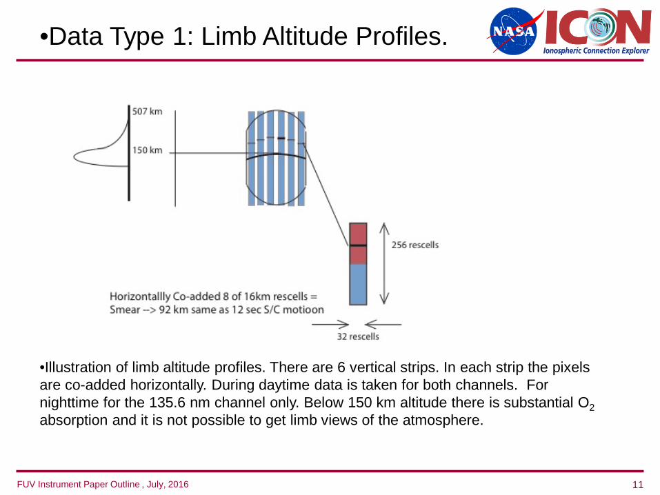
•Data Type 1: Limb Altitude Profiles.
•Illustration of limb altitude profiles. There are 6 vertical strips. In each strip the pixels are co-added horizontally. During daytime data is taken for both channels. For nighttime for the 135.6 nm channel only. Below 150 km altitude there is substantial O2absorption and it is not possible to get limb views of the atmosphere.

FUV Instrument Paper Outline , July, 2016 12
Limb Altitude Profiles
Daytime for both channels. Nightime 135.6 nm only. Below 150 km altitude there is substantial O2 absorption and it is not possible to get limb views of the atmosphere.
ICON prime science is measuring the altitude distribution of the thermosphere/ionosphere on a spatial scale of ~ 500 km.
The nighttime equatorial ionosphere is often unstable producing small scale structures.
ICON will have the capability of monitoring the ionosphere to detect ionospheric irregularities on a spatial scale of 10-20 km.
ICON FUV has the capability of recoding images using Time Delay Integration (TDI)

FUV Instrument Paper Outline , July, 2016 13
Data Type 2: TDI-ed emission maps (Nightime only)
This treatment assumes that the emissions are mapped either on the sub-limb at a constant altitude at 300 km or on the limb view tangent point associated with the elevation of the view angle.

FUV Instrument Paper Outline , July, 2016 14
•Illustration of ICON operations (Side View)
FUV observes on the left (port) side of ICON. On the limb the maximum emission is seen at the tangent point.At sub limb height integrated emissions are observed•During daytime-
• ICON FUV takes only altitude profiles at limb tangents (no sub-limb).
• ICON looks perpendicular to the orbit plane• Exposures are 12 seconds long.• In 12 sec exposure ICON travels 96 km and the curvature of
the Earth will provide less than 1 km altitude error.

FUV Instrument Paper Outline , July, 2016 15
TDI imaging 0 turret angleRaw images white checks 0.6 counts per res cell per frame. Black 0.03 counts per frame.
Movie of uncorrected frames Co-added uncorrected images
Sub Limb
TDI mapped images with motion compensation co-added
Limb Tangent

FUV Instrument Paper Outline , July, 2016 16
TDI imaging 15 degree turret angleRaw images sublimb white 0.6 counts per res cell per frame. Black 0.03 counts per frame.
Movie of uncorrected frames Co-added uncorrected images
Sub Limb
TDI mapped images with motion compensation co-added
Limb Tangent

FUV Instrument Paper Outline , July, 2016 17
Calibrated LBH & 135.6 intensities
Limb Profile Limb Profile TDI limb TDI sublimb
LBH day 135.6 135.6 135.6
FUV Data Products
LEVEL 2
LEVEL 3
LEVEL 1b
[O]/[N2] Nighttime O+
O/N2 map Nightime O+ Nighttime O+
Limb map Sub Limb Map
Nighttime O+ Tomographic Map Inversions

FUV Instrument Paper Outline , July, 2016 18
Atmospheric model for straylight calculations.
Constructed source models for limb emission derived from GUVI from measurements from atmospheric vs. altitude for 121.6 nm, 130.4 nm, 135.6 nm, 157 nm
Completed preliminary atmospheric limb irradiance calculations for both cameras at 121.6 nm, 130.4 nm, 135.6 nm, 157 nm157 nm source model used LBH lines at 153.1 nm, 155.8 nm, 158.6 nm, 160.2

FUV Instrument Paper Outline , July, 2016 19
GUVI data of the key day-glow features.
FUV Instrument Paper Outline , July, 2016 20
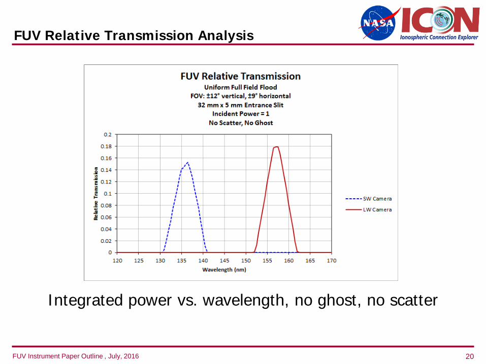
FUV Relative Transmission Analysis
Integrated power vs. wavelength, no ghost, no scatter

FUV Instrument Paper Outline , July, 2016 21
Reference Intensity vs. Altitude
Notes GUVI data was used for the 121.6 nm, 130.4 nm, and 135.6 nm source models (all traced
monochromatically) The 157 nm (LW) source model is polychromatic, with in-band wavelengths selected from the Meier
spectrum data. It uses the LBH1 limb profile.
•LW source wavelengths

FUV Instrument Paper Outline , July, 2016 22
Backgrounds
Modeling of stray light.Step 1. Performing PSD computations.- Instrument Response to parallel incoming radiation as a function of the angle of arrival at the aperture of the instrument.Step 2. Modeling the Limb. - Calculating the integrated stray light energy using the the PSD combined with the distribution of photon fluxes arriving at the aperture of the instrument. 2 component to stray light:1. Out of wavelength band radiation originating in the FOV2. In wavelength band radiation originating outside the FOV.

FUV Instrument Paper Outline , July, 2016 23
SW Camera PST (135.6 nm)
•Design wavelength
FUV Instrument Paper Outline , July, 2016 24
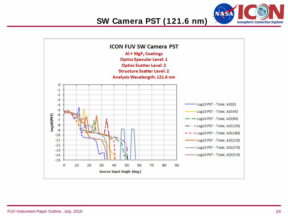
SW Camera PST (121.6 nm)

FUV Instrument Paper Outline , July, 2016 25
SW Camera PST (130.4 nm)

FUV Instrument Paper Outline , July, 2016 26
SW Camera PST (500 nm)
FUV Instrument Paper Outline , July, 2016 27
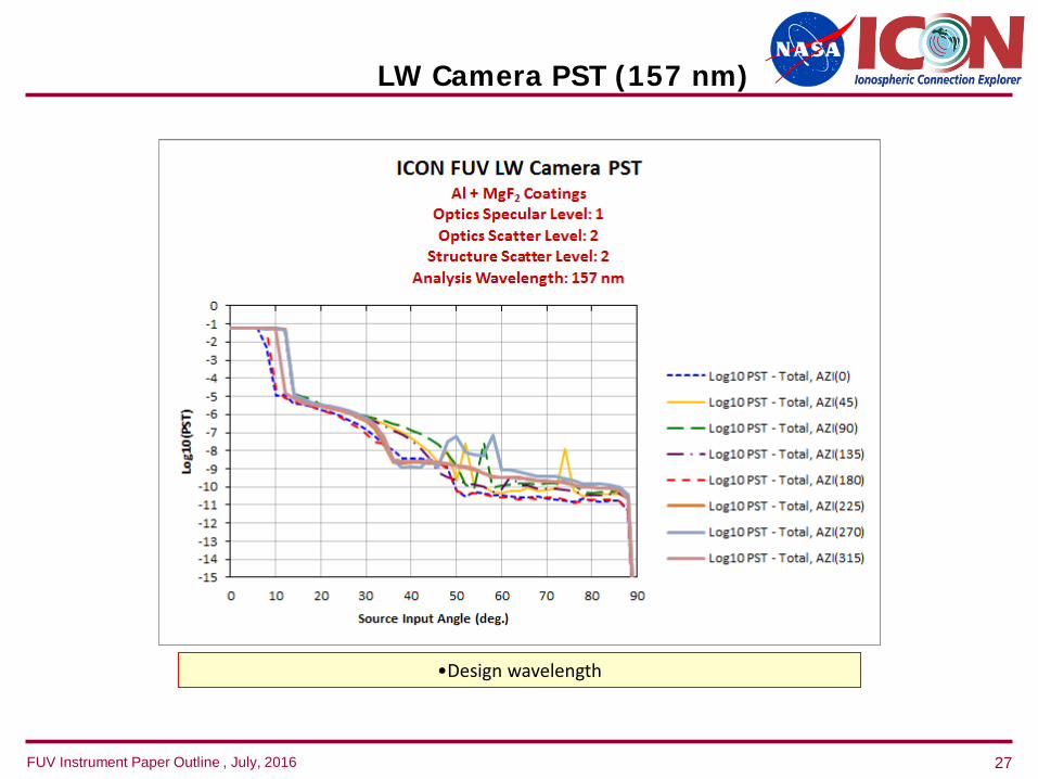
LW Camera PST (157 nm)
•Design wavelength

FUV Instrument Paper Outline , July, 2016 28
LW Camera PST (121.6 nm)

FUV Instrument Paper Outline , July, 2016 29
LW Camera PST (149.3 nm)

FUV Instrument Paper Outline , July, 2016 30
Modeling the Limb
Source radiance models are converted to intensity (flux/steradian) via ray tracing The trace algorithm divides the atmosphere into a series of earth-centric annular
rings corresponding to different altitudes Each ring is oriented so that it is tangent to the line of sight for a known altitude For reference the center of the field of view is tangent at an altitude of approximately 155
km As the altitude increases, the ring rotate away from the spacecraft equivalent to
increasing the vertical field angle Ray powers are computed using the limb radiance and line of sight projections
onto the baffle input Rays are traced to the aperture and the intensity values are computed on polar
grids that are subsequently used to in the source models for the detector irradiance computations

FUV Instrument Paper Outline , July, 2016 31
Comments
Visible light analysis (400 nm – 700 nm) shows nearly identical behavior for the two camerasNo diffraction: all light is propagated in the direction of the zeroth order (higher orders are evanescent)~7 orders of magnitude attenuation for objects inside the field of viewNo contribution outside of the field of view
Broadband coating results in higher backgrounds for out of band light It remains to be seen if this has a significant impact on the overall performance of the system
FUV Instrument Paper Outline , July, 2016 32
Comments
Because the SNR calculations are based on irradiance calculations, they are subject to statistical noise these data should not be interpreted as absolute, but should provide a good qualitative estimate of performance
Integrated flux calculations are more reliable in a ray trace, power converges more quickly than irradiance
Both SW and LW channels are susceptible to direct illumination from sources outside of the design field of view this contribution is a significant source of stray light
Out of band rejection is very good, even for cases in which the line strength is much larger than the intended signal
Ghost and scatter events, in and out of band, contribute a small amount to the stray light background
The model assumes a diffuse black surface treatment for all opto-mechanical surfaces and structures

FUV Instrument Paper Outline , July, 2016 33
Model by Photon Engineering Calculated PST based on instrument model Used GUVI measurements for daytime stray
light input and integrated PST Results better than 2% peak requirement Very effective out of band rejection especially
in the visible ~7 orders Dominant stray light from in band out of FOV
Scattering Analysis Summary
SW Camera LW camera
Signal (photons/s) 1.51E+07 9.42E+06
In band SL (photons/s) 1.47E+05 7.92E+04
In band SL (%) 0.98% 0.84%Out of band SL
(photons/s) 4.50E+04 3.43E+04
Out of band SL (%) 0.30% 0.36%
Total SL (%) 1.27% 1.20%
Requirement: scattered light all contribution < 2%

FUV Instrument Paper Outline , July, 2016 34
Atmospheric model for straylight calculations.
Constructed source models for limb emission derived from GUVI from measurements from atmospheric vs. altitude for 121.6 nm, 130.4 nm, 135.6 nm, 157 nm
Completed preliminary atmospheric limb irradiance calculations for both cameras at 121.6 nm, 130.4 nm, 135.6 nm, 157 nm157 nm source model used LBH lines at 153.1 nm, 155.8 nm, 158.6 nm, 160.2

FUV Instrument Paper Outline , July, 2016 35
SW Camera: Signal Irradiance

FUV Instrument Paper Outline , July, 2016 36
SW Camera: Background Irradiance
•In band stray light, all angles
•Out of band, all angles
•Plots not on same scale
FUV Instrument Paper Outline , July, 2016 37
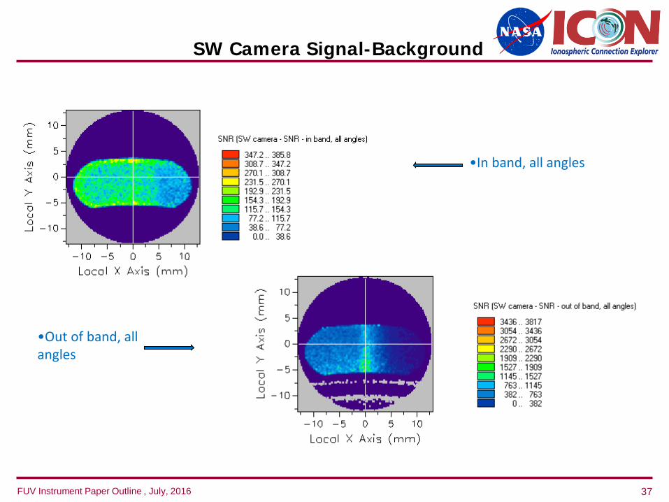
SW Camera Signal-Background
•In band, all angles
•Out of band, all angles
•Plots not on same scale

FUV Instrument Paper Outline , July, 2016 38
LW Camera: Signal Irradiance
FUV Instrument Paper Outline , July, 2016 39
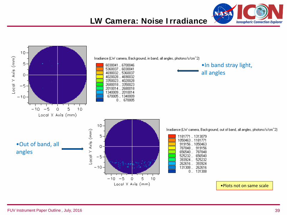
LW Camera: Noise Irradiance
•In band stray light, all angles
•Out of band, all angles
•Plots not on same scale
FUV Instrument Paper Outline , July, 2016 40
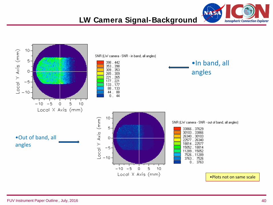
LW Camera Signal-Background
•Out of band, all angles
•Plots not on same scale
•In band, all angles

FUV Instrument Paper Outline , July, 2016 41
Comments
Because the SNR calculations are based on irradiance calculations, they are subject to statistical noise these data should not be interpreted as absolute, but should provide a good qualitative estimate of performance
Integrated flux calculations are more reliable in a ray trace, power converges more quickly than irradiance
Both SW and LW channels are susceptible to direct illumination from sources outside of the design field of view this contribution is, by far, the most significant source of stray light
Out of band rejection is very good, even for cases in which the line strength is much larger than the intended signal
Ghost and scatter events, in and out of band, contribute a small amount to the stray light background
The model assumes a diffuse black surface treatment for all opto-mechanical surfaces and structures

FUV Instrument Paper Outline , July, 2016 42
Prior estimates (ICON CSR) the requirement S-3 needs an instrument of sensitivity 8.3 counts/kR/sec.
Daytime O/N2 Ratio LW Sensitivity Requirement
The analysis of the O/N2 requirements was revisited since PDR (R. Meier private communication) preliminary results show that the L4 requirement is conservative.
New analysis includes (1) Slit widening, and (2) Recalculated effective N2 branching ratios (3) More realistic error assessment.

FUV Instrument Paper Outline , July, 2016 43
Signal to Noise•Area: A res cell is equivalent to 4 km altitude and 128 km horizontal. CCD is read out in a 512 x 512 raster - res cell is equivalent to 2 x 64 CCD binned pixel.• Time: We will consider a 12 second exposure.• Reference point. Signal and Noise reference point is at the CCD before the A-D converter and unit is electron which is 1/16th of the A-D in the SDL GSE.
•
•Where P = Signal in counts in the area collected during exposure time.• g = gain of the intensifier• Ip=stray light induced in counts• Nr=read out noise• Ndc = dark current of CCD•
•Most quantities are measured using the detector prototype. Mean Gain =645 Mean square = 734
y=40*(20+x/100)*EXP(-(((x/100-5.5)/5.5)^2))

FUV Instrument Paper Outline , July, 2016 44
Signal to Noise Ratio SummaryInput quantities.
signal, P 30 Rayleighs 8.82counts/pixel in stripe
Poisson fluctuations noise=sqrt(P) 2.97 ideal
Gain, g 645 A/D units 1.03E+04 Measuredsignal 9.11E+04 elecctrons
Mean square gain 1.17E+04 EstimatedIntensifer background 10 counts/sec/all pixels 0.01953125 electronsCCD read out noise 40 per frame 1280 electrons
Component Final Result No Mult. NoiseSignal 9.11E+04 9.11E+04P x mean g^2 1.22E+09 9.41E+08Ip x mean g^2 2.70E+06 2.70E+06Nr 2.56E+06 2.56E+06Ndc 3.75E+04 3.75E+04Dark current fluctuations 9.22E+07 9.22E+07Mean square 1.31E+09 1.04E+09RMS noise (CCD els) 3.63E+04 3.22E+04
RMS noise (PE-s) 3.51 3.12
• Nighttime SNR input = 30 Rayleighs.
• Instrument sensitivity 135.6 per stripe = 24.5 counts/sec/kR.
• Signal is amplified by intensifier gain.
• Photo electron noise and backgrounds are amplified by mean square intensifier gain.
• Noise components are summed as squares.
• CCD dark current and CCD read out noise are added.
• The ideal per rescel in each strip noise would be 2.97 but the resulting noise is 3.51.
• The largest contributor is multiplication noise.

FUV Instrument Paper Outline , July, 2016 45
Coarse mechanical alignment using Faro Arm CMM. Benchtop alignment of spectrometer and back imager using a
GSE visible grating @ 900 line/mm (UV is 3600 line/mm) and CCD detectors. Initial alignment at Lockheed Martin, Palo AltoRepeat post-ship at CSL in Liege, Belgium
Alignment of turret to optics package using laser tracker system.
Visible alignment with turret using CSL OGSE and MGSE. UV alignment using CSL OGSE and MGSE. UV Calibration at RT, 0C and 40C using CSL OGSE, MGSE,
and Thermal Tent.
Alignment and Calibration Approach

FUV Instrument Paper Outline , July, 2016 46
Benchtop Alignment at LMSAL

FUV Instrument Paper Outline , July, 2016 47
CSL MGSE Overview
FUV
•UV Flight CameraVertical axis
Horizontal axis
2 axis of rotation (vertical + horizontal)

FUV Instrument Paper Outline , July, 2016 48
Collimated beam does not cover the entire surface of the scan mirror
For one specific field, the turret does not need to befully illuminated
Collimated beam: 100 mm diameter
•Collimated beam
CSL OGSE Overview

FUV Instrument Paper Outline , July, 2016 49
Distortion Map Calibration
Alpha Beta Alpha Beta Alpha Beta0 11 2 4 6 -4-5 10 6 4 -8 -85 10 -8 0 -4 -8-8 8 -4 0 0 -8-4 8 0 0 4 -80 8 4 0 8 -84 8 8 0 -5 -108 8 -6 -4 5 -10-6 4 -2 -4 0 -11-2 4 2 -4
Post environmental calibration map: 29 points minimum
Pre environmental calibration map: 9 points
Alpha is the horizontal angle along the spectral directionBeta is the vertical angle along the slit

FUV Instrument Paper Outline , July, 2016 50
Spot sized optimized by actuating CM2 mirrors in piston/tip/tilt at the (0,0) field.
Extreme field angles at FOV edges verified and optimized following (0,0) field optimization.
All fields show spots meet requirements (<180 microns, >90% encircled energy)
UV Alignment Results
Reqt < 3.9pixels Reqt < 3.9pixels
Reqt > 90%Reqt > 90%

FUV Instrument Paper Outline , July, 2016 51•Alliant Techsystems Proprietary/Export Controlled
Shortwave (135.6 nm)
Longwave (157 nm)
Spectral Sensitivity at 20C
In-Band Suppression of 130.4 line is 100% in SW Channel
In-Band Suppression of 149.6 and 164.1 lines is >99.8% in LW Channel

FUV Instrument Paper Outline , July, 2016 52
Distortion mapping SW field positions measured during tests at different temperaturesColors denote tests:Blue: Cold GradientLight green: Hot GradientDark green: Room TemperatureBrown: 0 CRed: 40 CSpots are on top of each other within 2 pixels (1 science pixel in final 256x256 science format)

FUV Instrument Paper Outline , July, 2016 53
Images at 74 field positionsDistortion Map Determination
Uncorrected Distortion Map Corrected Distortion Map
Distortion Map Applied to Entire FOV

FUV Instrument Paper Outline , July, 2016 54
Initial out of band sensitivity measurements were performed at Lyman Alpha with high flux from the CSL OGSE. A well focused spot was observed in both channels.
Expected rejection at this wavelength was 105, ~103 was observed:
Following the initial tests, BaF2 windows were installed onto the OGSE. These filters are known to have rejection >90% at wavelengths less than 130nm. Spectral scans were performed with and without the BaF2 windows installed.
Out of Band Sensitivity at Lyman Alpha (1 of 2)
LWSW

FUV Instrument Paper Outline , July, 2016 55
Both channels showed a reduction in counts consistent with BaF2 Transmission curves (knee is ~135 nm at room temperature) indicating that in-band light was leaking from the monochromator into the OGSE.
Out of Band Sensitivity at Lyman Alpha (2 of 2)
72% in LW throughput with BaF2 installed0% to 60% in SW throughput
with BaF2 installed

FUV Instrument Paper Outline , July, 2016 56
Radiometric performance Summary
Radiometric Performance
Measured instrumental Transmission 0.45% 0.16%Count Rate from measured Tx 147.26 52.36 Counts/kRBOL from measured Tx 88.80 30.21 Counts/kREOL from measured Tx 75.84 25.55 Counts/kRScience Requirments 13.00 8.30 Counts/kRMargin BOL 583% 264% MarginMargin EOL 483% 208% Margin