The - IARIA Journals · Mario Freire, University of Beira Interior, Portugal Carlos Becker...

The International Journal on Advances in Networks and Services is published by IARIA.

ISSN: 1942-2644

journals site: http://www.iariajournals.org

contact: [email protected]

Responsibility for the contents rests upon the authors and not upon IARIA, nor on IARIA volunteers,

staff, or contractors.

IARIA is the owner of the publication and of editorial aspects. IARIA reserves the right to update the

content for quality improvements.

Abstracting is permitted with credit to the source. Libraries are permitted to photocopy or print,

providing the reference is mentioned and that the resulting material is made available at no cost.

Reference should mention:

International Journal on Advances in Networks and Services, issn 1942-2644

vol. 9, no. 3 & 4, year 2016, http://www.iariajournals.org/networks_and_services/

The copyright for each included paper belongs to the authors. Republishing of same material, by authors

or persons or organizations, is not allowed. Reprint rights can be granted by IARIA or by the authors, and

must include proper reference.

Reference to an article in the journal is as follows:

<Author list>, “<Article title>”

International Journal on Advances in Networks and Services, issn 1942-2644

vol. 9, no. 3 & 4, year 2016, <start page>:<end page> , http://www.iariajournals.org/networks_and_services/

IARIA journals are made available for free, proving the appropriate references are made when their

content is used.

Sponsored by IARIA

www.iaria.org

Copyright © 2016 IARIA

International Journal on Advances in Networks and Services

Volume 9, Number 3 & 4, 2016

Editor-in-Chief

Tibor Gyires, Illinois State University, USA

Editorial Advisory Board

Mario Freire, University of Beira Interior, PortugalCarlos Becker Westphall, Federal University of Santa Catarina, BrazilRainer Falk, Siemens AG - Corporate Technology, GermanyCristian Anghel, University Politehnica of Bucharest, RomaniaRui L. Aguiar, Universidade de Aveiro, PortugalJemal Abawajy, Deakin University, AustraliaZoubir Mammeri, IRIT - Paul Sabatier University - Toulouse, France

Editorial Board

Ryma Abassi, Higher Institute of Communication Studies of Tunis (Iset'Com) / Digital Security Unit, TunisiaMajid Bayani Abbasy, Universidad Nacional de Costa Rica, Costa RicaJemal Abawajy, Deakin University, AustraliaJavier M. Aguiar Pérez, Universidad de Valladolid, SpainRui L. Aguiar, Universidade de Aveiro, PortugalAli H. Al-Bayati, De Montfort Uni. (DMU), UKGiuseppe Amato, Consiglio Nazionale delle Ricerche, Istituto di Scienza e Tecnologie dell'Informazione (CNR-ISTI),ItalyMario Anzures-García, Benemérita Universidad Autónoma de Puebla, MéxicoPedro Andrés Aranda Gutiérrez, Telefónica I+D - Madrid, SpainCristian Anghel, University Politehnica of Bucharest, RomaniaMiguel Ardid, Universitat Politècnica de València, SpainValentina Baljak, National Institute of Informatics & University of Tokyo, JapanAlvaro Barradas, University of Algarve, PortugalMostafa Bassiouni, University of Central Florida, USAMichael Bauer, The University of Western Ontario, CanadaCarlos Becker Westphall, Federal University of Santa Catarina, BrazilZdenek Becvar, Czech Technical University in Prague, Czech RepublicFrancisco J. Bellido Outeiriño, University of Cordoba, SpainDjamel Benferhat, University Of South Brittany, FranceJalel Ben-Othman, Université de Paris 13, FranceMathilde Benveniste, En-aerion, USALuis Bernardo, Universidade Nova of Lisboa, PortugalAlex Bikfalvi, Universidad Carlos III de Madrid, SpainThomas Michael Bohnert, Zurich University of Applied Sciences, SwitzerlandEugen Borgoci, University "Politehnica"of Bucharest (UPB), RomaniaFernando Boronat Seguí, Universidad Politecnica de Valencia, SpainChristos Bouras, University of Patras, GreeceMahmoud Brahimi, University of Msila, AlgeriaMarco Bruti, Telecom Italia Sparkle S.p.A., ItalyDumitru Burdescu, University of Craiova, Romania

Diletta Romana Cacciagrano, University of Camerino, ItalyMaria-Dolores Cano, Universidad Politécnica de Cartagena, SpainJuan-Vicente Capella-Hernández, Universitat Politècnica de València, SpainEduardo Cerqueira, Federal University of Para, BrazilBruno Chatras, Orange Labs, FranceMarc Cheboldaeff, T-Systems International GmbH, GermanyKong Cheng, Vencore Labs, USADickson Chiu, Dickson Computer Systems, Hong KongAndrzej Chydzinski, Silesian University of Technology, PolandHugo Coll Ferri, Polytechnic University of Valencia, SpainNoelia Correia, University of the Algarve, PortugalNoël Crespi, Institut Telecom, Telecom SudParis, FrancePaulo da Fonseca Pinto, Universidade Nova de Lisboa, PortugalOrhan Dagdeviren, International Computer Institute/Ege University, TurkeyPhilip Davies, Bournemouth and Poole College / Bournemouth University, UKCarlton Davis, École Polytechnique de Montréal, CanadaClaudio de Castro Monteiro, Federal Institute of Education, Science and Technology of Tocantins, BrazilJoão Henrique de Souza Pereira, University of São Paulo, BrazilJavier Del Ser, Tecnalia Research & Innovation, SpainBehnam Dezfouli, Universiti Teknologi Malaysia (UTM), MalaysiaDaniela Dragomirescu, LAAS-CNRS, University of Toulouse, FranceJean-Michel Dricot, Université Libre de Bruxelles, BelgiumWan Du, Nanyang Technological University (NTU), SingaporeMatthias Ehmann, Universität Bayreuth, GermanyWael M El-Medany, University Of Bahrain, BahrainImad H. Elhajj, American University of Beirut, LebanonGledson Elias, Federal University of Paraíba, BrazilJoshua Ellul, University of Malta, MaltaRainer Falk, Siemens AG - Corporate Technology, GermanyKároly Farkas, Budapest University of Technology and Economics, HungaryHuei-Wen Ferng, National Taiwan University of Science and Technology - Taipei, TaiwanGianluigi Ferrari, University of Parma, ItalyMário F. S. Ferreira, University of Aveiro, PortugalBruno Filipe Marques, Polytechnic Institute of Viseu, PortugalUlrich Flegel, HFT Stuttgart, GermanyJuan J. Flores, Universidad Michoacana, MexicoIngo Friese, Deutsche Telekom AG - Berlin, GermanySebastian Fudickar, University of Potsdam, GermanyStefania Galizia, Innova S.p.A., ItalyIvan Ganchev, University of Limerick, IrelandMiguel Garcia, Universitat Politecnica de Valencia, SpainEmiliano Garcia-Palacios, Queens University Belfast, UKMarc Gilg, University of Haute-Alsace, FranceDebasis Giri, Haldia Institute of Technology, IndiaMarkus Goldstein, Kyushu University, JapanLuis Gomes, Universidade Nova Lisboa, PortugalAnahita Gouya, Solution Architect, FranceMohamed Graiet, Institut Supérieur d'Informatique et de Mathématique de Monastir, TunisieChristos Grecos, University of West of Scotland, UKVic Grout, Glyndwr University, UKYi Gu, Middle Tennessee State University, USAAngela Guercio, Kent State University, USAXiang Gui, Massey University, New Zealand

Mina S. Guirguis, Texas State University - San Marcos, USATibor Gyires, School of Information Technology, Illinois State University, USAKeijo Haataja, University of Eastern Finland, FinlandGerhard Hancke, Royal Holloway / University of London, UKR. Hariprakash, Arulmigu Meenakshi Amman College of Engineering, Chennai, IndiaGo Hasegawa, Osaka University, JapanEva Hladká, CESNET & Masaryk University, Czech RepublicHans-Joachim Hof, Munich University of Applied Sciences, GermanyRazib Iqbal, Amdocs, CanadaAbhaya Induruwa, Canterbury Christ Church University, UKMuhammad Ismail, University of Waterloo, CanadaVasanth Iyer, Florida International University, Miami, USAPeter Janacik, Heinz Nixdorf Institute, University of Paderborn, GermanyImad Jawhar, United Arab Emirates University, UAEAravind Kailas, University of North Carolina at Charlotte, USAMohamed Abd rabou Ahmed Kalil, Ilmenau University of Technology, GermanyKyoung-Don Kang, State University of New York at Binghamton, USASarfraz Khokhar, Cisco Systems Inc., USAVitaly Klyuev, University of Aizu, JapanJarkko Kneckt, Nokia Research Center, FinlandDan Komosny, Brno University of Technology, Czech RepublicIlker Korkmaz, Izmir University of Economics, TurkeyTomas Koutny, University of West Bohemia, Czech RepublicEvangelos Kranakis, Carleton University - Ottawa, CanadaLars Krueger, T-Systems International GmbH, GermanyKae Hsiang Kwong, MIMOS Berhad, MalaysiaKP Lam, University of Keele, UKBirger Lantow, University of Rostock, GermanyHadi Larijani, Glasgow Caledonian Univ., UKAnnett Laube-Rosenpflanzer, Bern University of Applied Sciences, SwitzerlandGyu Myoung Lee, Institut Telecom, Telecom SudParis, FranceShiguo Lian, Orange Labs Beijing, ChinaChiu-Kuo Liang, Chung Hua University, Hsinchu, TaiwanWei-Ming Lin, University of Texas at San Antonio, USADavid Lizcano, Universidad a Distancia de Madrid, SpainChengnian Long, Shanghai Jiao Tong University, ChinaJonathan Loo, Middlesex University, UKPascal Lorenz, University of Haute Alsace, FranceAlbert A. Lysko, Council for Scientific and Industrial Research (CSIR), South AfricaPavel Mach, Czech Technical University in Prague, Czech RepublicElsa María Macías López, University of Las Palmas de Gran Canaria, SpainDamien Magoni, University of Bordeaux, FranceAhmed Mahdy, Texas A&M University-Corpus Christi, USAZoubir Mammeri, IRIT - Paul Sabatier University - Toulouse, FranceGianfranco Manes, University of Florence, ItalySathiamoorthy Manoharan, University of Auckland, New ZealandMoshe Timothy Masonta, Council for Scientific and Industrial Research (CSIR), Pretoria, South AfricaHamid Menouar, QU Wireless Innovations Center - Doha, QatarGuowang Miao, KTH, The Royal Institute of Technology, SwedenMohssen Mohammed, University of Cape Town, South AfricaMiklos Molnar, University Montpellier 2, FranceLorenzo Mossucca, Istituto Superiore Mario Boella, ItalyJogesh K. Muppala, The Hong Kong University of Science and Technology, Hong Kong

Katsuhiro Naito, Mie University, JapanDeok Hee Nam, Wilberforce University, USASarmistha Neogy, Jadavpur University- Kolkata, IndiaRui Neto Marinheiro, Instituto Universitário de Lisboa (ISCTE-IUL), Instituto de Telecomunicações, PortugalDavid Newell, Bournemouth University - Bournemouth, UKArmando Nolasco Pinto, Universidade de Aveiro / Instituto de Telecomunicações, PortugalJason R.C. Nurse, University of Oxford, UKKazuya Odagiri, Yamaguchi University, JapanMáirtín O'Droma, University of Limerick, IrelandRainer Oechsle, University of Applied Science, Trier, GermanyHenning Olesen, Aalborg University Copenhagen, DenmarkJose Oscar Fajardo, University of the Basque Country, SpainConstantin Paleologu, University Politehnica of Bucharest, RomaniaEleni Patouni, National & Kapodistrian University of Athens, GreeceHarry Perros, NC State University, USAMiodrag Potkonjak, University of California - Los Angeles, USAYusnita Rahayu, Universiti Malaysia Pahang (UMP), MalaysiaYenumula B. Reddy, Grambling State University, USAOliviero Riganelli, University of Milano Bicocca, ItalyTeng Rui, National Institute of Information and Communication Technology, JapanAntonio Ruiz Martinez, University of Murcia, SpainGeorge S. Oreku, TIRDO / North West University, Tanzania/ South AfricaSattar B. Sadkhan, Chairman of IEEE IRAQ Section, IraqHusnain Saeed, National University of Sciences & Technology (NUST), PakistanAddisson Salazar, Universidad Politecnica de Valencia, SpainSébastien Salva, University of Auvergne, FranceIoakeim Samaras, Aristotle University of Thessaloniki, GreeceLuz A. Sánchez-Gálvez, Benemérita Universidad Autónoma de Puebla, MéxicoTeerapat Sanguankotchakorn, Asian Institute of Technology, ThailandJosé Santa, University Centre of Defence at the Spanish Air Force Academy, SpainRajarshi Sanyal, Belgacom International Carrier Services, BelgiumMohamad Sayed Hassan, Orange Labs, FranceThomas C. Schmidt, HAW Hamburg, GermanyHans Scholten, Pervasive Systems / University of Twente, The NetherlandsVéronique Sebastien, University of Reunion Island, FranceJean-Pierre Seifert, Technische Universität Berlin & Telekom Innovation Laboratories, GermanySandra Sendra Compte, Polytechnic University of Valencia, SpainDimitrios Serpanos, Univ. of Patras and ISI/RC ATHENA, GreeceRoman Y. Shtykh, Rakuten, Inc., JapanSalman Ijaz Institute of Systems and Robotics, University of Algarve, PortugalAdão Silva, University of Aveiro / Institute of Telecommunications, PortugalFlorian Skopik, AIT Austrian Institute of Technology, AustriaKarel Slavicek, Masaryk University, Czech RepublicVahid Solouk, Urmia University of Technology, IranPeter Soreanu, ORT Braude College, IsraelPedro Sousa, University of Minho, PortugalCristian Stanciu, University Politehnica of Bucharest, RomaniaVladimir Stantchev, SRH University Berlin, GermanyRadu Stoleru, Texas A&M University - College Station, USALars Strand, Nofas, NorwayStefan Strauβ, Austrian Academy of Sciences, AustriaÁlvaro Suárez Sarmiento, University of Las Palmas de Gran Canaria, SpainMasashi Sugano, School of Knowledge and Information Systems, Osaka Prefecture University, Japan

Young-Joo Suh, POSTECH (Pohang University of Science and Technology), KoreaJunzhao Sun, University of Oulu, FinlandDavid R. Surma, Indiana University South Bend, USAYongning Tang, School of Information Technology, Illinois State University, USAYoshiaki Taniguchi, Kindai University, JapanAnel Tanovic, BH Telecom d.d. Sarajevo, Bosnia and HerzegovinaOlivier Terzo, Istituto Superiore Mario Boella - Torino, ItalyTzu-Chieh Tsai, National Chengchi University, TaiwanSamyr Vale, Federal University of Maranhão - UFMA, BrazilDario Vieira, EFREI, FranceLukas Vojtech, Czech Technical University in Prague, Czech RepublicMichael von Riegen, University of Hamburg, GermanyYou-Chiun Wang, National Sun Yat-Sen University, TaiwanGary R. Weckman, Ohio University, USAChih-Yu Wen, National Chung Hsing University, Taichung, TaiwanMichelle Wetterwald, HeNetBot, FranceFeng Xia, Dalian University of Technology, ChinaKaiping Xue, USTC - Hefei, ChinaMark Yampolskiy, Vanderbilt University, USADongfang Yang, National Research Council, CanadaQimin Yang, Harvey Mudd College, USABeytullah Yildiz, TOBB Economics and Technology University, TurkeyAnastasiya Yurchyshyna, University of Geneva, SwitzerlandSergey Y. Yurish, IFSA, SpainJelena Zdravkovic, Stockholm University, SwedenYuanyuan Zeng, Wuhan University, ChinaWeiliang Zhao, Macquarie University, AustraliaWenbing Zhao, Cleveland State University, USAZibin Zheng, The Chinese University of Hong Kong, ChinaYongxin Zhu, Shanghai Jiao Tong University, ChinaZuqing Zhu, University of Science and Technology of China, ChinaMartin Zimmermann, University of Applied Sciences Offenburg, Germany

International Journal on Advances in Networks and Services

Volume 9, Numbers 3 & 4, 2016

CONTENTS

pages: 38 - 48A System for Managing Transport-network Recovery Using Hybrid-backup Operation Planes according toDegree of Network FailureToshiaki Suzuki, Hitachi, Ltd., JapanHiroyuki Kubo, Hitachi, Ltd., JapanHayato Hoshihara, Hitachi, Ltd., JapanKenichi Sakamoto, Hitachi, Ltd., JapanHidenori Inouchi, Hitachi, Ltd., JapanTaro Ogawa, Hitachi, Ltd., Japan

pages: 49 - 59A Scalable and Dynamic Distribution of Tenant Networks across Multiple Provider Domains usingCloudcastingKiran Makhijani, Huawei Technologies, United StatesRenwei Li, Huawei Technologies, United StatesLin Han, Huawei Technologies, United States

pages: 60 - 70Device Quality Management for IoT Service Providers by Tracking Uncoordinated Operating HistoryMegumi Shibuya, KDDI Research, Inc., JAPANTeruyuki Hasegawa, KDDI Research, Inc., JAPANHirozumi Yamaguchi, Osaka University, JAPAN

pages: 71 - 82SDN Solutions for Switching Dedicated Long-Haul Connections: Measurements and Comparative AnalysisNageswara Rao, Oak Ridge National Laboratory, USA

pages: 83 - 95A Model for Managed Elements under Autonomic Cloud Computing ManagementRafael de Souza Mendes, Federal University of Santa Catarina, BrazilRafael Brundo Uriarte, IMT School for Advanced Studies Lucca, ItalyCarlos Becker Westphall, Federal University of Santa Catarina, Brazil

pages: 96 - 106Multiradio, Multiboot capable sensing systems for Home Area NetworkingBrendan O'Flynn, Tyndall National Institute, University College Cork, IrelandMarco DeDonno, Tyndall National Institute, University College Cork, IrelandWassim Magnin, Tyndall National Institute, University College Cork, Ireland

pages: 107 - 116Analyzing the Performance of Software Defined Networks vs Real NetworksJose M. Jimenez, Universidad Politécnica de Valencia, SpainOscar Romero, Universidad Politécnica de Valencia, SpainAlbert Rego, Universidad Politécnica de Valencia, SpainJaime Lloret, Universidad Politécnica de Valencia, Spain

38

International Journal on Advances in Networks and Services, vol 9 no 3 & 4, year 2016, http://www.iariajournals.org/networks_and_services/

2016, © Copyright by authors, Published under agreement with IARIA - www.iaria.org

A System for Managing Transport-network Recovery

Using Hybrid-backup Operation Planes according to Degree of Network Failure

Toshiaki Suzuki, Hiroyuki Kubo, Hayato Hoshihara, and Kenichi Sakamoto

Research & Development Group Hitachi, Ltd.

Kanagawa, Japan E-mails: {toshiaki.suzuki.cs, hiroyuki.kubo.do,

hayato.hoshihara.dy, and kenichi.sakamoto.xj}@hitachi.com

Hidenori Inouchi and Taro Ogawa

Information & Telecommunication Systems Company Hitachi, Ltd.

Kanagawa, Japan E-mails: {hidenori.inouchi.dw and

taro.ogawa.tg}@hitachi.com

Abstract—A system for managing transport-network recovery using hybrid-backup operation planes according to the degree of a network failure is proposed. Under this management system, an entire network is separated into multiple areas. A network-management server prepares a three-step recovery procedure to cover the degree of network failure. In the first step of the recovery, an inside-area protection scheme is used to recover current data-transmission paths in each area. In the second step, an end-to-end protection scheme is applied to the current data-transmission paths. In the third step, the operation plane is changed. Each assumed operation plane is composed of recovery configurations for restoring failure paths for assumed area-based network failures. If a small network failure occurs, it is recovered by the inside-area protection and end-to-end protection schemes. If a catastrophic network failure (caused by a disaster) that cannot be recovered by those protection schemes occurs, it is recovered by changing the operation plane in accordance with the damaged areas. A prototype system composed of a network-management server and 96 emulated packet-transport nodes was developed and evaluated by configuring 1000 data-transmission paths. In case of a small network failure, 500 data-transmission paths were damaged, and they were reconfigured by the inside-area protection scheme and end-to-end protection scheme in about 5 seconds. If the network failure was not recovered by those protection schemes, 1000 data-transmission paths were reconfigured in about 1.2 seconds after the network-management server decided to change the operation plane. As a result, the proposed system could localize a network failure and recover a transport network according to the degree of network failures.

Keywords - network management; protection; disaster recovery; packet transport

I. INTRODUCTION

Lately, reflecting the rapid growth of the Internet and cloud systems, various services, for example, on-line shopping, net banking, and social-networking services (SNSs), are being provided via networks. Under these circumstances, networks have become an indispensable service supporting daily life. If a network is out of service due to failures of network nodes, people’s lives and

businesses would be considerably damaged. Therefore, if a network fails, it should be recovered promptly. Failures of a network can be envisioned as “small” failures (such as a failure of a node or a link) or “extensive” failures (due to natural disasters). It is therefore a crucial issue to develop a scalable network-recovery scheme that can cover recovery from either a small network failure or a catastrophic network failure.

In our previous work presented at INNOV 2015 [1], an entire system architecture was focused on a scalable network-recovery scheme by extending a prior system [2]. In this extended work, a prototype system for multiple tenant users was implemented, and its performance was evaluated in comparison with a conventional system.

As recovery procedures for network failures, two major schemes [3], namely, “protection” and “restoration,” are utilized. As for protection, it is possible to recover from a network failure promptly because a backup path to a current path is prepared in advance. However, to recover from a network disaster, numerous backup paths must be prepared. Protection is therefore useful for small network failures. On the other hand, as for restoration, a recovery path is recalculated after a network failure is detected. It therefore takes much time to recover from a network failure if numerous current paths exist.

In light of the above-described issues, a robust network-management scheme is required. The overall aim of the present study is thus to develop a network-management scheme [1][2] for monitoring and controlling network resources so as to quickly restore network services after a network disaster.

The procedure for recovering from a network failure consists of three steps: the first step is to quickly detect a network failure; the second is to immediately determine how to recover from the failure; the third is to promptly configure recovery paths. The second step is focused on in the present study. In particular, a scalable network-recovery scheme—covering failures ranging from small ones to extensive ones—is proposed. The target network is a transport network, such as a Multi-Protocol Label

39



Switching - Transport Profile (MPLS-TP) network. The rest of this paper is organized as follows. Section II

describes related work. Section III overviews a previously proposed system and a requirement to apply it to not only catastrophic failures but also small network failures. Section IV proposes a new network-disaster recovery system. Sections V and VI respectively describe an architecture of a prototype system and present some results of evaluations of the system’s performance. Section VII concludes the paper.

II. RELATED WORK

Several standardization activities related to reliable networks have been ongoing. The International Telecommunication Union - Telecommunication Standardization Sector (ITU-T) [4] discussed specifications, such as Transport – Multi Protocol Label Switching (T-MPLS), in the first stage of standardization. In the next stage, the ITU-T jointly standardized MPLS-TP specifications with the Internet Engineering Task Force (IETF) [5]. Requests for comments (RFC) on requirements [6] and a framework [7] for MPLS-TP were then issued. In addition, RFCs on a framework for MPLS-TP-related operation, administration, and maintenance (OAM) [8] and survivability [9] were issued. Based on the OAM framework, the previously proposed system can detect network failures promptly.

Several schemes for failure recovery have been proposed. One major scheme, called “fast reroute” [10], prepares a back-up path. Another recovery scheme (for multiple failures) prepares multiple backup paths [11], and another one prepares a recovery procedure for multiple modes [12]. In the case of these protection schemes, to recover from a catastrophic network failure, a huge volume of physical resources for preparing a large number of standby paths is needed. These schemes are useful for limited network failures, namely failures of a few links or nodes.

In the case of restoration schemes, in contrast to protection schemes, recovery paths are calculated after a network failure is detected. Restoration schemes for handling multiple failures [13] and virtual networks [14] have been proposed. A scheme for reducing search ranges by using landmark nodes has also been proposed [15]. It is useful for recovering a seriously damaged network, since all reroutes are calculated after a failure is detected. However, if a large number of current paths exist, it might take much time to calculate all recovery paths.

III. PREVIOUS SYSTEM AND REQUIREMENTS

The previously proposed network-recovery system is shown in Figure 1 [2]. The target network is composed of packet transport nodes (PTNs), such as those in an MPLS-TP network. The system only focuses on recovery from multiple area-based network failures on PTN networks. A critical issue in the case of a network disaster is the time consumed in recovering the numerous established paths

(shown as solid blue arrows) in packet networks. (Note that “path” means a label-switched path (LSP) [16] and a pseudo wire (PW) [17].) A user is connected to one of the PTNs through a network such as an IP network. A server located in a data center (DC) is also connected to one of the PTNs through an IP network.

The previously proposed system could promptly recover from a catastrophic failure of a network by using prepared back-up paths (shown as dotted red arrows). However, it significantly changes network configurations, even if a network failure is small, since network conditions are managed on the basis of divided network areas. It must therefore be enhanced so that it can recover from a catastrophic network failure, as well as a small network failure, by using fewer configurational changes based on the degree of damage due to the network failure.

User Data center

NW area(1)

NW area(2)

NW area(3) NW area

(4)

NW area(5)

NW area(6)

NW area(7)

NW area(8)

Network-managementserver

PTN PTN

PTNPTN

PTN PTN

PTNPTN

PTN PTN

PTNPTN

PTN PTN

PTNPTN

PTN PTN

PTNPTN

PTN PTN

PTNPTN

PTN PTN

PTNPTN

PTN PTN

PTNPTN

Failure

Failure

PTN PTN

Figure 1. Previously proposed network-recovery system

IV. PROPOSED TRANSPORT NETWORK-RECOVERY

SCHEME

To meet the above-described requirements, a three-step recovery procedure for covering the degree of network failures is proposed. The first step of the procedure is to execute “an inside-area protection scheme” to recover small failures, such as a node failure in each area formed by separating an entire network into small areas. The second step is to execute “an end-to-end protection scheme” to recover small failures, such as a failure of a link between areas not recovered by the inside-area protection scheme. The third step is to execute “an operation-plane change scheme” to recover extensive failures, such as network failures of multiple areas.

A. Path protection for small network failures in each area

The proposed system should promptly recover a network from a small failure, such as a link failure between PTNs or a PTN failure. A scheme called “inside-area protection”—for localizing and swiftly recovering from a small network failure—is overviewed in Figure 2. Using a conventional scheme (such as cluster analysis), the network-management server divides an entire PTN network into multiple (e.g.,

40



eight) areas, which it then manages. It configures a current path (shown as solid black arrows in the figure), composed of a LSP and a PW, for transmitting data from a sender to a receiver according to requests by end users. The network-management server configures a backup path for each current path, namely, an inside-area protection path (shown as dotted red arrows), between one edge PTN and another edge PTN in every area. Specifically, the network-management server finds an edge PTN pair that is related to the current path in every area. For example, PTN 14 and PTN 11 are the edge PTN pair in area (1), since packet data from PE1 are received by PTN 14 and then transmitted to area (5) by PTN 11, as shown in Figure 4. In addition, PTN 54 and PTN 53, PTN 84 and PTN 83, and PTN 42 and PTN 43 are the edge PTN pairs that are related to the current path. The network-management server calculates a detour path for each edge PTN pair by excluding network links that are parts of the current path. For example, a detour path between PTN 14 and PTN 11 through PTN 13 and PTN 12 is calculated as the backup path. All calculated detour paths in each area become the inside-area protection paths.

In each area, both edge PTNs exchange OAM packets to check if a disconnection exists between the PTNs. If a disconnection is detected, they send an alert to the network-management server, which keeps the received alert and monitors the degree of failures, namely, numbers of link and PTN failures, and damaged areas.

In the case shown in Figure 2, a link failure between PTN 14 and PTN 11 is assumed to occur in area (1). PTN 14 and PTN 11 detect the link failure, which is recovered by the inside-area protection. Specifically, a direct data-transmission path from PTN 14 to PTN 11 is changed to a backup transmission path through PTN 13 and PTN 12. On the other hand, the path between PTN 14 and PTN 11 is a part of an end-to-end path between provider-edge 1 (PE1) and PE2. The link failure between PTN 14 and PTN 11 is therefore temporarily detected by PE1 and PE2, since both PEs also exchange OAM packets. However, both PEs wait for 100 milliseconds to see whether the link failure is recovered by the inside-area protection. Therefore, when the link failure is recovered by the inside-area protection, neither PE executes further recovery action.

User Data center

NW area(1)

NW area(2)

NW area(3) NW area

(4)

NW area(5)

NW area(6)

NW area(7)

NW area(8)


54 53

5251

14 13

1211

64 63

6261

24 23

2221

34 33

3231

44 43

4241

84 83

8281

74 73

7271

Failure

PE2PE1

Figure 2. Configuration of path protection in each NW area

B. End-to-end path protection for small network failures

The proposed system should be able to immediately recover from a small failure that is not recovered by the above-described protection (such as a link failure between areas). A scheme called “end-to-end protection” to promptly recover from a failure that is not restored by the inside-area protection is overviewed as follows. The network-management server configures a backup path (called an “end-to-end protection path”) for each current path between PE1 and PE2. PEs exchange OAM packets to check whether a disconnection exists between them.

Specifically, as shown in Figure 3, the network-management server configures a current path (shown as solid black arrows) between PE1 and PE2 [through areas (1), (5), (8), and (4)] for transmitting data packets between a user and a DC. In addition, the network-management server configures a backup path called an “end-to-end protection path (shown as dotted red arrows)” between PE1 and PE2. The end-to-end protection path is established so as not to travel through the same areas used by the current path as much as possible. In Figure 3, the backup path is configured to transmit data through areas (2), (6), (7), and (3).

During network operation, the end-to-end protection is executed when the data transmission between PEs is disconnected for a while (for example, 100 milliseconds). In the case of Figure 3, a link failure between areas (5) and (8) is assumed. This failure is not recovered by the inside-area protection; instead, it is recovered by the end-to-end protection because it occurs between areas. Specifically, a data-transmission path is changed from the current path (shown as solid black arrows) to a backup path (shown as dotted red arrows).

The end-to-end protection scheme is similar to a conventional protection scheme. In the case of a conventional scheme, the protection is immediately executed after one of the PEs detects a disconnection. However, in the case of the proposed end-to-end protection scheme, it is not executed for 100 milliseconds so that it can be checked whether a failure has been recovered by the inside-area protection or not.

User Data center

NW area(1)

NW area(2)

NW area(3) NW area

(4)

NW area(5)

NW area(6)

NW area(7)

NW area(8)


54 53

5251

14 13

1211

64 63

6261

24 23

2221

34 33

3231

44 43

4241

84 83

8281

74 73

7271

Failure

PE2PE1

Figure 3. Configuration of path protection for end-to-end transmission

41



C. Changing operation plane for network-disaster recovery

The proposed system should be able to promptly recover not only failures inside a network area and between network areas but also catastrophic failures. A recovery scheme that changes the operation plane to recover from area-based network failures is overviewed in Figure 4. Before starting network operations, the network-management server prepares multiple backup operation planes for handling possible area-based network failures. Each backup operation plane is composed of recovery configurations for restoring failure paths due to assumed network failures. During network operation, if network failures are not recovered by both the inside-area protection and the end-to-end protection, the failures are recovered by changing an operation plane.

User Data center

NW area(1)

NW area(2)

NW area(3) NW area

(4)

NW area(5)

NW area(6)

NW area(7)

NW area(8)


54 53

5251

14 13

1211

64 63

6261

24 23

2221

34 33

3231

44 43

4241

84 83

8281

74 73

7271

Failure Failure

Failure Failure

PE2PE1

Figure 4. Configuration for changing an operation plane for network-

disaster recovery

In Figure 4, as an example, the network-management

server configures multiple currents paths [through areas (1), (5), (8), and (4)] for transmitting data packets between a user and a DC. It calculates all recovery paths preliminarily by assuming all possible area-based network failures. The number of possible combinations of areas is 256 (i.e., 28), and it includes a pattern by which no area-based network failure occurs. The network-management server therefore prepares 255 backup operation planes. It then assigns a unique recovery identifier (ID) for each backup operation plane, and sends all recovery IDs and recovery configurations to each PTN, which stores all received recovery IDs and configurations.

An example area-based network-failure recovery procedure is shown in Figure 4. In the figure, area-based network failures are assumed to occur in areas (1), (4), (6), and (7). In this case, PE1 (namely, an edge node of the current path) detects a disconnection between PE1 and PE2. PE1 waits 100 milliseconds to check whether the failures are recovered by the inside-area protection. It also checks the availability of the end-to-end protection path (which is not shown in Figure 4) by using OAM packets. If the failures are not recovered in 100 milliseconds and the end-to-end protection path is not available, PE1 sends an alert to the network-management server to inform it that the end-to-

end protection is not available. The network-management server then checks which areas are not available. In this example, by receiving many alerts sent by multiple PTNs, the network-management server determines that area-based network failures occur in areas (1), (4), (6), and (7). By using the determined network-failure information, it then determines the most suitable backup operation plane to recover. To change an operation plane, the network-management server sends a recovery ID specifying the most-suitable backup operation plane to related PTNs, which change data transmissions according to the received recovery ID. By means of the above-described procedures, the operation plane is changed, and catastrophic network failures are swiftly recovered.

V. ARCHITECTURE OF PROTOTYPE SYSTEM

In this section, the architecture of a prototype system is described. Specifically, the structure of the prototype system is shown first. Then, recovery procedures are overviewed. After that, calculation procedures for the inside-area protection paths and the end-to-end protection paths are described. (Note that calculation procedures for the backup operation planes are not described since they are explained in a previous work [2].) At the end of this section, an implemented viewer is depicted.

A. Structure of prototype system

A prototype system was implemented by using three servers. The structure of the prototype system—composed of an application server, a control server, and a node simulator server—is shown in Figure 5. Specifically, implemented software components are shown in the figure.

The application server is in charge of the entire network management. Specifically, it manages calculation and configuration of current paths and protection paths by sending commands. In addition, it calculates and configures back-up operation planes with multiple detour paths by assuming possible node failures or area-based network failures. Besides, it receives alerts and determines the degree of network failures. It then selects a recovery back-up operation plane and sends it an identifier specifying it to network nodes.

The control server is in charge of transmitting command messages from the application server to the simulator server. Specifically, it receives calculated route information of the current paths, protection paths, and back-up operation planes and distributes it to the simulated multiple network nodes. In addition, it monitors state of connections between not only current paths but also protection paths. When it detects a disconnection, it prompts the node simulator server to activate an alert. On the other side, it transmits alert information from the simulator server to the application server.

42



Simulator server

DB

Viewer

Application server Interface for viewer

Configurationmanagement

Alertmonitor

Pathmanagement

Modelmanagement

Alert-informationmanagement

Alertreceiver

Configurationsender

Commandsender

Control server

Network nodeAlert

managementAlert

activationCommandreceiver

Configurationmanagement

Alert-informationmanagement

Alertsender

Configurationreceiver

Commandreceiver

Alertreceiver

Alertmanagement

Commandsender

Modelmanagement

Connection monitor

Figure 5. Structure of prototype system

The simulator server emulates certain parts of the

functions of MPLS-TP network nodes. It receives configurations of LSP and PW paths and sets data-transmission paths on the basis of the received path information. When it is requested to activate alerts, it sends an SNMP trap to the control server.

B. Overview of recovery procedures

The structure of the proposed transport network-recovery scheme is similar to the previously proposed scheme (shown in Figure 1). Namely, it is composed of a network-management sever and multiple PTNs. The network-management server centrally manages the whole network. However, the recovery procedures differ from those of the previous system.

Start

Divide a whole network into areas

Calculate inside-area protection paths for each area

Calculate all end-to-end protection paths

Set calculated path configurations

Calculate operation planes for all possible area-failure patterns

Calculate current paths (LSPs and PWs)

Receive failures?

Monitor network failures

No

Determine a failure type

Recover from failures

Yes

Figure 6. Overview of proposed recovery procedure

A flow chart of the new recovery procedure is shown in Figure 6. First, after starting a network-management function, the network-management server divides the whole network into multiple areas. It calculates current paths (composed of LSPs and PWs) for transmitting data from a sender node to a receiver node according to inputs by a network manager. The network-management server calculates “inside-area protection paths” for each area and “end-to-end protection paths” to recover current paths in case of network failures. In addition, it calculates virtual operation planes for all possible area-failure patterns. The protection paths and virtual operation planes are described in detail in later sections. The network-management server sets the entire configuration of the calculated paths to all network nodes and starts to monitor the network for failures. When it detects a network failure, it determines the type of failure, namely, an area-based or node-based failure. The network-management server then executes the appropriate failure-recovery procedures according to the determined failure degree.

C. Calculation of inside-area protection paths

An implemented flow chart of the calculation procedure of inside-area protection paths is shown in Figure 7.

No

No

Start

Select a current path without inside-area protection

Select an area where inside-area protection is not set

Select two edge nodes on the current path in the area

Calculate an inside-area protection path between the two edge nodes

Are inside-area protection paths calculated for the current path ?

Are inside-area protection paths for all current paths calculated ?

End

Yes

YesConfigure all calculated inside-protection paths

Figure 7. Calculation procedure for inside-area protection paths

The application server selects a current path that does not

have an inside-area protection path. In addition, it selects an area where inside-area-protection for the selected current path is not set. Then, it selects two edge nodes on the selected current path in the selected area. One is the start point and the other is the end point for the selected path in the selected area. The application server calculates the inside-area protection path between the two selected edge nodes and stores it. After that, it checks whether the inside-area protection paths related to the selected current path are calculated or not. If they are calculated, it checks whether

43



all inside-area protection paths for all current paths are calculated or not. If they are not calculated, it calculates other inside-area protection paths for the remaining current paths. If all inside-area protection paths are calculated and stored, it terminates the calculation procedures.

D. Calculation of end-to-end protection paths

An implemented flow chart of the calculation procedure for end-to-end protection paths is shown in Figure 8. The application server selects a current path that does not have an end-to-end protection path. In addition, it sets a high cost value for links in areas that the current path passes through. It then calculates an end-to-end protection path for the selected current path to minimize the cost of the summation of the links composing the protection path. After that, it checks whether all end-to-end protection paths for all current paths are calculated or not. If they are not calculated, it calculates other end-to-end protection paths for the remaining current paths. If they are calculated and stored, it terminates the calculation procedure.

Start

Select a current path without end-to-end protection path

Set high cost value for links in areas where the current path goes through

Calculate an end-to-end protection path for the current path

Are end-to-end protection paths for all current paths calculated ?

No

End

YesConfigure all calculated end-to-end

protection paths

Figure 8. Calculation procedure for end-to-end protection paths

E. Calculation of recovery paths for operation-plane change

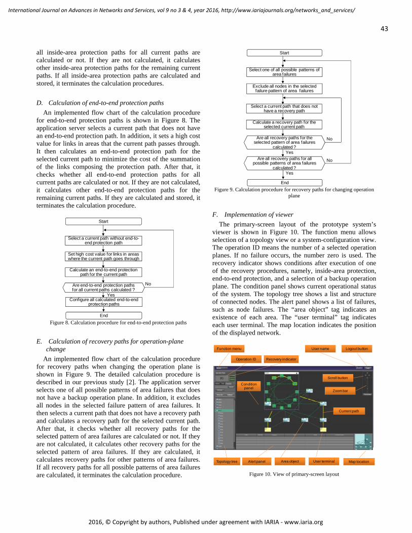
An implemented flow chart of the calculation procedure for recovery paths when changing the operation plane is shown in Figure 9. The detailed calculation procedure is described in our previous study [2]. The application server selects one of all possible patterns of area failures that does not have a backup operation plane. In addition, it excludes all nodes in the selected failure pattern of area failures. It then selects a current path that does not have a recovery path and calculates a recovery path for the selected current path. After that, it checks whether all recovery paths for the selected pattern of area failures are calculated or not. If they are not calculated, it calculates other recovery paths for the selected pattern of area failures. If they are calculated, it calculates recovery paths for other patterns of area failures. If all recovery paths for all possible patterns of area failures are calculated, it terminates the calculation procedure.

Start

Exclude all nodes in the selected failure pattern of area failures

Are all recovery paths for the selected pattern of area failures

calculated ?

No

End

Yes

Select one of all possible patterns of area failures

Select a current path that does not have a recovery path

Calculate a recovery path for the selected current path

Are all recovery paths for all possible patterns of area failures

calculated ?

No

Yes

Figure 9. Calculation procedure for recovery paths for changing operation

plane

F. Implementation of viewer

The primary-screen layout of the prototype system’s viewer is shown in Figure 10. The function menu allows selection of a topology view or a system-configuration view. The operation ID means the number of a selected operation planes. If no failure occurs, the number zero is used. The recovery indicator shows conditions after execution of one of the recovery procedures, namely, inside-area protection, end-to-end protection, and a selection of a backup operation plane. The condition panel shows current operational status of the system. The topology tree shows a list and structure of connected nodes. The alert panel shows a list of failures, such as node failures. The “area object” tag indicates an existence of each area. The “user terminal” tag indicates each user terminal. The map location indicates the position of the displayed network.

Function menu

Recovery indicator

User name Logout button

Alert panel Map location

Operation ID

Scroll button

Zoom bar

User terminalArea object

Current path

Topology tree

Conditionpanel

Figure 10. View of primary-screen layout

44



The “current path” tag highlights the currently used path. The “zoom bar” button provides a function to change the size of the displayed network. The “scroll” button provides a function to change the position of the displayed network. The “user name” tag shows the name of a current user. The “logout” button is used to terminate network management.

VI. PERFORMANCE EVALUATION AND RESULTS

The above-described recovery procedures were evaluated in the case of a small network failure and a catastrophic network failure by using the prototype system. In the evaluation, the times needed to calculate and to configure a table for current data-transmission paths (composed of PWs and LSPs) were evaluated. In addition, the times taken to configure recovery paths in the case of a failure of a PTN or an area-based failure were evaluated.

A. Evaluation system

The system used for evaluating the proposed recovery procedures is shown in Figure 11. It is composed of a network-management server and 96 PTNs. As shown in the figure, an entire PTN network is divided into eight areas. Each network area is composed of 12 PTNs, as shown in NW area (7). In each area, PTNs are connected in a reticular pattern. In addition, each user terminal is connected to PTN-network areas (1) and (2) through PE1 or PE3, and each application server in DC1 or DC2 is connected to PTN-network areas (3) and (4) through PE2 or PE4.

Note that the PTN networks (composed of 96 PTNs) are emulated by a physical server. The user terminal and application server are also emulated by the physical server, whose specification is listed in Table I. Another physical server, which executes the network-management function, has the same specifications as the former server.

NW area(1)

NW area(2)

NW area(3) NW area

(4)

NW area(5)

NW area(6) NW area

(7)

NW area(8)


PTN PTN

PTNPTN

PTN PTN

PTNPTN

PTN PTN

PTNPTN

PTN PTN

PTNPTN

PTN PTN

PTNPTN

PTN PTN

PTNPTN

PTN PTN

PTNPTN

12 PTN 12 PTN 12 PTN 12 PTN

12 PTN 12 PTN

12 PTN

PTN

PTN

PTN

PTN

PTN

PTN

PTN

PTN

PTN

PTN

PTN

PTN

User 1 Data center 2

PE1 PE4

User 2

PE3

Data center 1

PE2

Figure 11. Evaluation system

TABLE I. SPECIFICATION OF SERVER # Item Specification 1 CPU 1.8 GHz, 4 cores 2 Memory 16 Gbytes 3 Storage 600 Gbytes

TABLE II. EVALUATED ITEMS # Item Evaluation specification1 Current-path calculation

timeTime to calculate 100 (=50+50), 500 (=250+250), and 1000 (=500+500) PWs

2 Current-path distribution time

Time to distribute all calculated current paths in case of 100 (=50+50), 500 (=250+250), and 1000 (=500+500) PWs

3 Protection-path calculation time for each area

Time to calculate all protection paths in each area for 100 (=50+50), 500 (=250+250), and 1000 (=500+500) PWs

4 Protection-path calculation time for end-to-end protection paths

Time to calculate all protection paths for all end-to-end current paths for 100 (=50+50), 500 (=250+250), and 1000 (=500+500) PWs

5 Recovery-path calculation time for changing operation plane

Time to calculate recovery 100 (=50+50), 500 (=250+250), and 1000 (=500+500) PWs for all possible area-failure patterns

6 Recovery-configuration time

Time to configure all protection paths after detecting path failures for 100 (=50+50), 500 (=250+250), and 1000 (=500+500) PWs

7 Recovery-ID distribution time

Time to distribute a recovery ID after detecting an area failure for 100 (=50+50), 500 (=250+250), and 1000 (=500+500) PWs

B. Evaluation conditions

The times taken to calculate multiple PWs between PE1 and PE2 and between PE3 and PE4 were evaluated. Each PW was included in a LSP. If a transmission path of a PW differed from the path of an already setup LSP, a new LSP was setup, and the PW was included in the new LSP. The evaluations were executed according to the patterns listed in Table II. Specifically, the times taken to calculate current paths, to distribute their configuration to all PTNs, and to calculate the inside-area protection paths and end-to-end protection paths were evaluated by changing the number of PWs (namely, 50+50, 250+250, and 500+500 for two users). In addition, the times taken to calculate recovery paths for changing the operation plane, to configure protection paths, and to distribute the recovery ID were evaluated.

C. Evaluation results

1) Current-path calculation time The times taken to calculate current PWs requested by

the two users are plotted in Figure 12. User 1 accesses a server in DC1 through PE1 and PE2. User 2 accesses a server in DC2 through PE3 and PE4. A scalability evaluation was executed by changing setup PWs for each user. As shown in the figure, the times taken to calculate 100 (=50+50) current PWs, 500 (=250+250) current PWs, and 1000 (=500+500) current PWs were respectively about 152, 570, and 1079 milliseconds.

45



2) Distribution time for configuring current paths The times taken to distribute all configurations of the

calculated current paths to all PTNs are plotted in Figure 13. As shown in the figure, the times taken to distribute all configurations of the 100 (=50+50) current PWs, 500 (=250+250) current PWs, and 1000 (=500+500) current PWs are respectively about 25, 330, and 923 milliseconds.

3) Protection-path calculation time for all current paths in each area

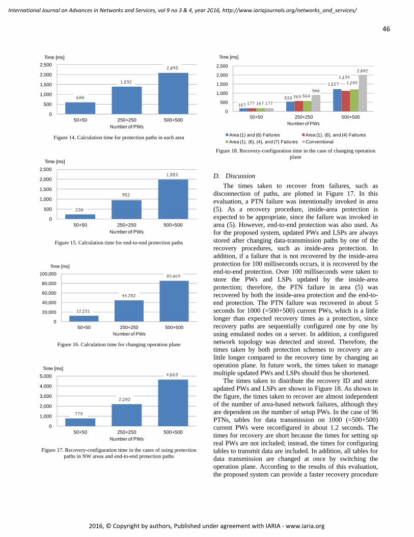
The times taken to calculate protection paths corresponding to all current PWs in each area are plotted in Figure 14. As shown in the figure, the times required for calculating all the inside-area protection paths for 100 (=50+50) current PWs, 500 (=250+250) current PWs, and 1000 (=500+500) current PWs are respectively about 600, 1392, and 2095 milliseconds.

4) Protection-path calculation time for all end-to-end current paths

The times taken to calculate end-to-end protection paths to all current PWs are plotted in Figure 15. As shown in the figure, the times taken to calculate all the end-to-end protection paths for 100 (=50+50) current PWs, 500 (=250+250) current PWs, and 1000 (=500+500) current PWs are respectively about 230, 952, and 1983 milliseconds.

5) Recovery-path calculation time for operation-plane change

The times taken to calculate all recovery PWs for 255 possible area-based network-failure patterns are plotted in Figure 16. As shown in the figure, the times taken to calculate all recovery PWs for 255 area-based network-failure patterns and 100 (=50+50) current PWs, 500 (=250+250) current PWs, and 1000 (=500+500) current PWs are respectively about 12.2, 44.8, and 85.5 seconds.

6) Recovery-configuration time required by both protection schemes for each area and end-to-end path

The times taken to set recovery configuration and to store a configured network topology by the inside-area protection and end-to-end protection schemes after detecting a path disconnection are plotted in Figure 17. Specifically, recovery configuration time was evaluated by intentionally invoking a node failure in area (5). In this case, half of the PWs were damaged and recovered. In the evaluation, if a disconnected path is not recovered for 100 milliseconds by the inside-area protection, it is automatically recovered by the end-to-end protection. Actually, disconnected paths were recovered by the end-to-end protection. As shown in the figure, the times to set recovery configurations for 100 (=50+50) current PWs, 500 (=250+250) current PWs, and 1000 (=500+500) current PWs by both protections are respectively about 0.8, 2.2, and 4.7 seconds.

7) Recovery-ID distribution time for changing operation plane

The times taken to distribute the recovery ID to related PTNs and recover after the last area-based network failure is detected in the case of 100 (=50+50) current PWs, 500 (=250+250) current PWs, and 1000 (=500+500) current PWs

are plotted in Figure 18. Three area-based network-failure patterns, namely, failures of network areas (1) and (6), failures of network areas (1), (6), and (4), and failures of network areas (1), (6), (4), and (7), were evaluated. As shown in the figure, in the case of 100 (=50+50) current PWs, the times taken to recover from the last failure for the three area-based network-failure patterns are respectively about 167, 177, and 167 milliseconds. In the case of 500 (=250+250) current PWs, the times taken to recover from the last failure for the three area-based network-failure patterns are respectively about 533, 569, and 564 milliseconds. In the case of 1000 (=500+500) current PWs, the times taken to recover from the last failure for the three area-based network-failure patterns are respectively about 1227, 1134, and 1205 milliseconds. As a result, tables that are used for data transmission on 1000 (=500+500) PWs are reconfigured by changing an operation plane in about 1.2 seconds.

In Figure 18, the proposed method is compared with a conventional restoration method in terms of the time taken to calculate and configure PWs. With the conventional method, the times to set recovery configurations for 100 (=50+50) current PWs, 500 (=250+250) current PWs, and 1000 (=500+500) current PWs are respectively about 177, 900, and 2002 milliseconds.

0

200

400

600

800

1,000

1,200

50+50 250+250 500+500

Number of PWs

現用系パスの算出時間(2NW)

152

570

1,079

Time [ms]

Figure 12. Calculation time for current paths

0

200

400

600

800

1,000

50+50 250+250 500+500

Number of PWs

現用系パスの設定時間(2NW)

25

330

923

Time [ms]

Figure 13. Distribution time for current-path configuration

46



0

500

1,000

1,500

2,000

2,500

50+50 250+250 500+500

Number of PWs

エリア内プロテクション・パス算出時間(2NW)

600

1,392

2,095

Time [ms]

Figure 14. Calculation time for protection paths in each area

0

500

1,000

1,500

2,000

2,500

50+50 250+250 500+500

Number of PWs

端点プロテクション・パス算出時間(2NW)

230

952

1,983

Time [ms]

Figure 15. Calculation time for end-to-end protection paths

0

20,000

40,000

60,000

80,000

100,000

50+50 250+250 500+500

Number of PWs

全復旧面の算出時間(2NW)Time [ms]

12,231

44,782

85,469

Figure 16. Calculation time for changing operation plane

0

1,000

2,000

3,000

4,000

5,000

50+50 250+250 500+500

Number of PWs

エリア内Ｐ+端点間Ｐ動作時間(2NW)

779

2,202

Time [ms]4,663

Figure 17. Recovery-configuration time in the cases of using protection

paths in NW areas and end-to-end protection paths

0

500

1,000

1,500

2,000

2,500

50+50 250+250 500+500

Number of PWs

面切替えのみの動作時間（2NW）

Area (1) and (6) Failures Area (1), (6), and (4) Failures

Area (1), (6), (4), and (7) Failures Conventional

167 167533

1,227

1,134

177

569 564

1,205

Time [ms]

177

900

2,002

Figure 18. Recovery-configuration time in the case of changing operation

plane

D. Discussion

The times taken to recover from failures, such as disconnection of paths, are plotted in Figure 17. In this evaluation, a PTN failure was intentionally invoked in area (5). As a recovery procedure, inside-area protection is expected to be appropriate, since the failure was invoked in area (5). However, end-to-end protection was also used. As for the proposed system, updated PWs and LSPs are always stored after changing data-transmission paths by one of the recovery procedures, such as inside-area protection. In addition, if a failure that is not recovered by the inside-area protection for 100 milliseconds occurs, it is recovered by the end-to-end protection. Over 100 milliseconds were taken to store the PWs and LSPs updated by the inside-area protection; therefore, the PTN failure in area (5) was recovered by both the inside-area protection and the end-to-end protection. The PTN failure was recovered in about 5 seconds for 1000 (=500+500) current PWs, which is a little longer than expected recovery times as a protection, since recovery paths are sequentially configured one by one by using emulated nodes on a server. In addition, a configured network topology was detected and stored. Therefore, the times taken by both protection schemes to recovery are a little longer compared to the recovery time by changing an operation plane. In future work, the times taken to manage multiple updated PWs and LSPs should thus be shortened.

The times taken to distribute the recovery ID and store updated PWs and LSPs are shown in Figure 18. As shown in the figure, the times taken to recover are almost independent of the number of area-based network failures, although they are dependent on the number of setup PWs. In the case of 96 PTNs, tables for data transmission on 1000 (=500+500) current PWs were reconfigured in about 1.2 seconds. The times for recovery are short because the times for setting up real PWs are not included; instead, the times for configuring tables to transmit data are included. In addition, all tables for data transmission are changed at once by switching the operation plane. According to the results of this evaluation, the proposed system can provide a faster recovery procedure

47



than recalculating and transmitting recovery paths to PTNs (since it omits the recalculation process).

In summary, a transport-network-recovery management system, which can recover from both a small network failure and a major network disaster, was proposed and evaluated. Specifically, for small failures, inside-area protection and end-to-end protection were proposed. In addition, for major failures, an area-based recovery procedure was proposed. As described above, updated data-transmission paths of PWs and LSPs are always stored in a database. Therefore, transmission paths composed of PWs and LSPs updated by changing the operation plane are also stored in the database. As a result, the times taken to recover from the network disaster by changing the operation plane depend on the number of PWs. However, as shown in Figures 16 and 17, the proposed system could promptly recover from both a small network failure and a catastrophic network failure (which is not covered by conventional network-recovery schemes).

VII. CONCLUTION

A system for managing transport-network recovery based on the degree of network failures is proposed. Under this management scheme, an entire network is separated into multiple areas. A network-management server executes a three-step recovery procedure. In the first step, an inside-area protection scheme is applied to the current data-transmission path in each area. In the second step, an end-to-end protection scheme is applied to the current data-transmission path. In the third step, the operation plane is changed. Each assumed operation plane is composed of recovery configurations for restoring failure paths under the assumption of area-based network failures. If a small network failure occurs, it is recovered and localized by the inside-area protection and end-to-end protection schemes. If a catastrophic network failure (due to a disaster) that is not recovered by the protection schemes occurs, it is recovered by changing the operation plane according to damaged areas.

A prototype system composed of a network-management server and 96 emulated packet-transport nodes was developed and evaluated by configuring 1000 (=500+500) data-transmission paths. In the case of a small network failure, 500 data-transmission paths composed by LSPs and PWs were damaged and reconfigured by the inside-area protection and end-to-end protection schemes in about 5 seconds. If a network failure was not recovered by the protection schemes, all tables for 1000 (=500+500) data transmission paths were reconfigured to recover from the failure by changing the operation plane in about 1.2 seconds. As a result, the proposed system could provide a faster recovery procedure than recalculating and transmitting recovery paths to PTNs. In addition, it could localize and recover a network failure according to the degree of network failures.

Although the protection scheme could recover 500 data

transmission paths from a small network failure, it took the network-management server about 5 seconds to configure and store changed-data transmission paths. If numerous current paths exist, it will take too much time to assess changed paths. Accordingly, the protection scheme will be further developed so that it can promptly manage a large number of recovered paths.

ACKNOWLEDGMENTS

Part of this research was done within research project O3 (Open, Organic, Optima) and programs, "Research and Development on Virtualized Network Technology," "Research and Development on Management Platform Technologies for Highly Reliable Cloud Services," and "Research and Development on Signaling Technologies of Network Configuration for Sustainable Environment" supported by MIC (The Japanese Ministry of Internal Affairs and Communications).

REFERENCES

[1] T. Suzuki et al., “A system for managing transport-network recovery according to degree of network failure,” The Fourth International Conference on Communications, Computation, Networks and Technologies (INNOV 2015), Nov. 2015, pp. 56-63.

[2] T. Suzuki et al., “A network-disaster recovery system using multiple-backup operation planes,” International Journal on Advances in Networks and Services, vol. 8 nos. 1&2, July 2015, pp. 118-129.

[3] E. Mannie and D. Papadimitriou, “Recovery (Protection and Restoration) Terminology for Generalized Multi-Protocol Label Switching (GMPLS),” IETF RFC 4427, Mar. 2006.

[4] International Telecommunication Union - Telecommunication Standardization Sector (ITU-T) http://www.itu.int/en/ITU-T/Pages/default.aspx [retrieved: Nov. 2016].

[5] The Internet Engineering Task Force (IETF), http://www.ietf.org/ [retrieved: Nov. 2016].

[6] B. Niven-Jenkins, D. Brungard, M. Betts, N. Sprecher, and S. Ueno, “Requirements of an MPLS transport profile,” IETF RFC 5654, Sept. 2009.

[7] M. Bocci, S. Bryant, D. Frost, L. Levrau, and L. Berger, “A Framework for MPLS in transport networks,” IETF RFC 5921, July 2010.

[8] T. Busi and D. Allan, “Operations, administration, and maintenance framework for MPLS-based transport neworks,” IETF RFC 6371, Sept. 2011.

[9] N. Sprecher and A. Farrel, “MPLS transport profile (MPLS-TP) survivability framework,” IETF RFC 6372, Sept. 2011.

[10] P. Pan, G. Swallow, and A. Atlas, “ Fast reroute extensions to RSVP-TE for LSP tunnels,” IETF RFC 4090, May 2005.

[11] J. Zhang, J. Zhou, J. Ren, and B. Wang, “A LDP fast protection switching scheme for concurrent multiple failures in MPLS network,” 2009 MINES '09. International

48



Conference on Multimedia Information Networking and Security, Nov. 2009, pp. 259-262.

[12] Z. Jia and G. Yunfei, “Multiple mode protection switching failure recovery mechanism under MPLS network,” 2010 Second International Conference on Modeling, Simulation and Visualization Methods (WMSVM), May 2010, pp. 289-292.

[13] M. Lucci, A. Valenti, F. Matera, and D. Del Buono, “Investigation on fast MPLS restoration technique for a GbE wide area transport network: A disaster recovery case,” 12th International Conference on Transparent Optical Networks (ICTON), Tu.C3.4, June 2010, pp. 1-4.

[14] T. S. Pham. J. Lattmann, J. Lutton, L. Valeyre, J. Carlier, and D. Nace, “A restoration scheme for virtual networks using

switches,” 2012 4th International Congress on Ultra Modern Telecommunications and Control Systems and Workshops (ICUMT), Oct. 2012, pp. 800-805.

[15] X. Wang, X. Jiang, C. Nguyen, X. Zhang, and S. Lu, “Fast connection recovery against region failures with landmark-based source routing,” 2013 9th International Conference on the Design of Reliable Communication Networks (DRCN), Mar. 2013, pp. 11-19.

[16] E. Rosen, A. Viswanathan, and R. Callon, “Multiprotocol lable switching architecture,” IETF RFC 3031, Jan. 2001.

[17] S. Bryant and P. Pate, “Pseudo wire emulation edge-to-edge (PWE3) architecture,” IETF RFC 3985, Mar. 2005.

49



A Scalable and Dynamic Distribution of Tenant Networksacross Multiple Provider Domains using Cloudcasting

Kiran Makhijani, Renwei Li and Lin Han

Future Networks, America Research CenterHuawei Technologies Inc., Santa Clara, CA 95050

Email: kiran.makhijani, renwei.li, lin.han@ {huawei}.com

Abstract—Network overlays play a key role in the adoption ofcloud oriented networks, which are required to scale and growelastically and dynamically up/down and in/out, be provisionedwith agility and allow for mobility. Cloud oriented networksspan over multiple sites and interconnect using Virtual PrivateNetwork (VPN) like services across multiple domains. Theseconnections are extremely slow to provision and difficult tochange. Current solutions to support cloud based networksrequire combination of several protocols in data centers andacross provider networks to implement end to end virtual networkconnections using different overlay technologies. However, theystill do not necessarily meet all the above requirements withoutadding operational complexity or without new modificationsto base protocols. This paper discusses a converged networkvirtualization framework called Cloudcasting, which is a singletechnology for virtual network interconnections within and acrossmultiple sites. The protocol is based on minimal control planesignaling and offers a flexible data plane encapsulation. Thebiggest challenge yet for any virtual network solution is todistribute and inter-connect virtual networks at global scaleacross different geographies and heterogeneous infrastructures.Data center operators are faced with the predicament to re-designnetworks in order to support a specific virtualization approach.Cloudcasting technology can be easily adopted to interconnect orextend virtual networks with in a massive scale software defineddata centers, campus networks, public, private or hybrid cloudsand even container environments with no change to physicalnetwork environment and without compromising simplicity.

Keywords–Network Overlay; Network Virtualization; Routing,Multi-Tenancy Virtual Data Center; VXLAN; BGP; EVPN.

I. INTRODUCTION

The Cloud adoption continues to grow; there is an upwardtrend of applications and services being built in platformindependent manner and the scope of connectivity is no longerlimited to a single site or a fixed location. As the cloud basedapplications evolve, the isolated operation and management oftenant networks (sharing common network access) that hostthese application becomes extremely complex and is differentthan the underlying physical networks. While infrastructurenetworks focus on delivering basic functions to ensure thatthe physical links are reliably available and reachable; thetenants concern with mechanisms to allocate and/or withdrawresources on-demand from different sites and network resourcepools. The leading requirement for tenants is to use the net-works in the most economical manner and still have sufficientresources available when needed.

The above mentioned motivation was first mentioned in theoriginal Cloudcasting paper [1], which described a network

virtualization framework that addresses many shortcomingsof existing solutions. The present paper expands on conceptsdescribed in the original paper and covers details about proto-type experiences, applications and advanced concepts of usingCloudcasting. Since the original work, we have observed thatthe Cloudcasting architecture applies to almost all virtualiza-tion scenarios and can be considered as a generalized frame-work for infrastructure indepedent virtual networking. Thelater sections of this paper further validates our observation.

The key characteristics of Cloud-oriented network ar-chitectures are resource virtualization, multi-site distribution,scalability, multi-tenancy and workload mobility. These aretypically enabled through network virtualization overlay tech-nologies. Initial network virtualization approaches relate tolayer-2 multi-path mechanisms such as, Shortest Path Bridging(SPB) [2] [3] and Transparent Interconnection of Lots of Links(TRILL) [4] to address un-utilized links and to limit broadcastdomains. Later, much of the focus was put into the data planeaspects of the network virtualization, for example, Virtual eX-tensible Local Area Networks (VXLAN) [5], Network Virtu-alization using Generic Routing Encapsulation (NVGRE) [6],and Generic Network Virtualization Encapsulation (GENEVE)[7]. These tunneling solutions provide the means to carry layer-2 and/or layer-3 packets of tenant networks over a sharedIP network infrastructure to create logical networks. Though,due to their lack of corresponding control plane schemes,the overall system orchestration and configuration becomescomplex for virtual network setup and maintenance [8].

Even more recently, MultiProtocol-Border Gateway Pro-tocol (MP-BGP) based Ethernet VPN (EVPN) [9] has beenproposed as a control plane for virtual network distribution,and has foundations of the VPN style provisioning model. Thisrequires additional changes to an already complex protocolthat was originally designed for the inter-domain routing. Thedeployment of MP-BGP/EVPN in data center networks alsobrings in corresponding bulky configurations, for example,defining Autonomous System (AS), that are not really relevantto the data center infrastructure network. The solutions likeTRILL, SPB and MP-BGP are a class of virtual network ar-chitectures that consume data structures of physical (substrate)network protocols, therefore, we refer to them as EmbeddedVirtual Networks. The term substrate network henceforth willbe used to describe a base, underlying, or an infrastructurenetwork upon which tenant networks are built as virtualnetwork overlays. Whereas Cloudcasting protocol is referred toas Extended Virtual Network because it inter-connects differenttypes of virtual networks through its own routing scheme. It

50



can be organized over any substrate network topology androuting arrangements. As a note to the reader, with in thescope of this document, a virtual, customer or tenant networkare used interchangeably and mean the same. A cloud is alocation and infrastructure network. A virtual network is anentity that shares physical network resources and access withother similar entities; virtual networks are isolated from eachother. In the context of this paper agility is understood asbeing able to responds to the changes in virtual network inreal time or as quickly as needed to best serve the customerexperience. Whereas elasticity refers to an ability to grow orshrink resource requirements on-demand.

Even though Embedded Virtual Network (the term isinspired from [10]) solutions mentioned above are quite func-tional, they are faced with several limitations. Of which themost significant and relevant to cloud-scale environments istheir dependence on the substrate networks. In addition tobeing scalable and reliable, a cloud scale network must also beelastic, dynamic, agile, infrastructure-independent, and capableof multi-domain support. There has not been any convergedarchitecture for network virtualization yet. In [1], we proposedCloudcasting, an Extended Virtual Network framework thatoperates on top of any substrate network and offers primitivesfor cloud auto-discovery, dynamic route distribution as needed.As an extension to original paper, several operational conceptshave been described. We have provided details of the prototypebut most important section deals with the scalable distributionof virtual networks across geographically remote sites.

The rest of the paper is organized as follows. We havekept Section II and III intact from original paper to introducethe reference model and its major functions. Section IVexplains different deployment scenarios where cloudcastingapplies to. While Section V discusses scalability at globallevel of the solution, Section VI introduces the Cloudcastingpolicy framework where in constraints on virtual networksmay be specified. Section VII has the qualitative analysisand implementation details and in Section VIII comparisonwith a few most common already existing solutions are made.Lastly, Section IX briefly lays out an interesting extension ofcloudcasting combining services and mobile networks.

II. CLOUDCASTING MODEL

A converged virtual routing scheme can be described bytwo primary factors; an infrastructure-independent virtual net-work framework, and a unified mechanism to build an overlayof various types of tenant networks with different addressschemes. On these basis, a new virtual routing scheme calledCloudcasting, is proposed with the following characteristics

1) Auto discovery: A signaling scheme that enables us toadd, delete, expand and virtualize a tenants networkwith minimum configuration.

2) Auto distribution: A signaling scheme that connectsmultiple virtual networks with each other or asym-metrically as needed.

3) Auto Scale: The ability to provide and serve highscale of tenants in a location-agnostic manner.

A cloudcasting network is an IP network, which is shared andused by multiple tenant clouds to route traffic within a singlevirtual network or between different virtual networks. We usethe terminology of tenant cloud to emphasize that a tenant or

Figure 1: Cloudcasting Reference Model.

Figure 2: Cloudcasting Framework.

a user network may reside anywhere on the substrate networkwith a highly dynamic routing table. The IP address space inone tenant cloud may overlap with that in another cloud andthese are not exposed to the shared IP infrastructure network.The cloudcasting reference model, is shown in Fig. 1. Eachcustomer has its own network shown as Tenant Cloud A, Band C, a shared substrate IP network that was built indepen-dently and can encompass multiple administrative domains.This model describes a centralized conversational scheme, inwhich tenant clouds or Virtual Extensible Networks (VXNs)announce their presence as well as membership interests toa centralized designated authority, called Cloudcasting Ren-dezvous Point (CRP), via a cloudcasting network virtualizationedge element called Cloudcasting Switching Point (CSP). Tocommunicate among the network elements, a new signal-ing protocol, called CloudCasting Control (CCC) protocol isdefined with three simple primitives facilitating cloud auto-discovery and cloud route distribution. The protocol primitivesare defined as below and are further illustrated in Fig. 2.

• Register message: A virtual network interest and self-identifying announcement primitive from CSP to CRP.

• Report message: A response from CRP to all CSPswith similar virtual network interests.

• Post message: A CSP to CSP virtual network routedistribution primitive.

The details of aforementioned cloudcasting network elementsand their properties in cloudcasting framework are discussedas below.

51



A. Virtual Extensible NetworkA Virtual Extensible Network is a tenant cloud or a user

network. It is represented by a unique identifier with a globalsignificance in cloudcasting network. Using this construct, itis possible to discover all its instances on the substrate IPfabric via CRP. VXN identifiers are registered with CRP fromCSPs to announce their presence. There are various possibleformats to define the VXN, for instance, an alphanumericvalue, number or any other string format. In the preliminarywork we have defined it as a named string that is mapped toa 28-bit integer identifier, thus enabling support for up to 256million clouds.

B. Cloud Switch PointA Cloud Switch Point is a network function that connects

virtual networks on one side to the substrate IP network on theother side. It can be understood as an edge of a virtual networkthat originates and terminates virtual tunnels. A CSP holdsmappings of L3 routes or L2 MAC forwarding informationof a virtual network. A CSP is cloudcasting equivalent of aVirtual Tunnel End Point (VTEP) [5] in VXLAN networks oran Ingress/Egress Tunnel Router (xTR) in the LISP domain[11] and may similarly be co-located with either on a serviceproviders edge (PE) router, on a top of rack (ToR) switch ina data center, or on both. A CSP participates in both auto-discovery and auto-route distribution. In order to establish aforwarding path between two endpoints of a virtual networkor of two different virtual networks, a CSP first registers withthe CRP its address and VXN identifiers it intends to connectto. Then the CRP will report to all CSPs that have interestin same VXN. Finally, the CSP will communicate with thoseother CSPs and exchange their routing information. On the dataforwarding plane, a CSP builds a virtual Forwarding Informa-tion Base (vFIB) table on per VXN basis and route/switchtraffic to the destination virtual networks accordingly.

C. Cloud Rendezvous PointA Cloud Rendezvous Point is a single logical entity that

stores, maintains and manages information about CSPs andtheir VXN membership. The CRP maintains the latest VXNto CSP membership database and distributes this informationto relevant CSPs so that they can form peer connectionand exchange virtual network routes automatically. A reportmessage is always generated whenever there is a change inthe virtual network membership database. However, CRP isoblivious to any change in vFIB (described above in CSP).

III. CLOUDCASTING COMMUNICATION PRIMITIVES

Now, we describe cloudcasting communication primitivesused among CRP and CSPs. Fig. 3 illustrates the layeringof the virtual routing over any substrate layer and overlaycontrol messages between CSP and CRP. The encapsulationmessage format is shown above in Fig. 4. A predefined TCPdestination port identifies the cloudcasting protocol and CCCheader contains the specification for the register, report andpost messages.

A. Cloudcasting Register MessageAn auto-discovery of virtual networks involves two mes-

sages. The first message is the Cloudcasting Register thatoriginates from CSPs to announce CSP is interested in a VXN

Figure 3: Cloudcasting Protocol Primitives

Figure 4: Cloudcasting Control Message Format

with the CRP. A Register message specification includes theCSP address and list of VXNs it is interested in. An interest isdefined as an intent to participate in a specific virtual network.For example, a vxnred on csp1 expresses interest to join vxnredon csp2. As an example, consider virtual networks vxnredand vxngreen are attached to csp1. Then, the register messagecontains a tuple as follows

Register{sender: csp1, [vxnred, vxngreen]}

After the CRP receives a cloudcasting register message,it scans its CSP membership database to look for the sameVXN identifiers. If it finds one (or more), a cloudcasting reportmessage is generated and sent to all the CSPs with sameinterest, otherwise, it simply logs the VXN in its CSP database.

B. Cloudcasting Report Message

The CRP generates cloudcasting report messages in re-sponse to a cloudcasting register message to inform CSPs ofother CSPs address and their associated VXN identifiers. If theCRP finds other CSP(s) with the same VXN membership (orinterested VXNs), then the Report messages are generated forthat CSP as well as the other found CSPs. A Report messageis sent to each CSP, that contains other CSP addresses for theshared VXNs. As an example, consider CRP already has csp2with interest in vxnred. Upon receiving a cloudcasting registermessage from csp1 as described earlier, two report messagesare generated as below for csp2 and csp1, respectively:

Report (csp2) {to: csp1, [interest: vxnred]}Report (csp1) {to: csp2, [interest: vxnred]}

52



Figure 5: Cloudcasting GVE Protocol Encapsulation

In this manner, auto-discovery of virtual network locationsis accomplished that is based on interest and announcementcriteria.

C. Cloudcasting Post MessageThe cloudcasting post messages facilitate route distribution

as needed. As a cloudcasting report message is received,the CSP will connect with other CSPs to exchange theirrouting information that includes VXN identifiers, a GenericVXN encapsulation (GVE) tag and the network reachabilityinformation within the VXN along with the address family.The list of network reachability information type includes butnot restricted to IP prefixes (such as, IPv4, IPv6), VLANs,MAC addresses or any other user defined address scheme. Asan example, when a report as described earlier is received,the following Post will originate from csp1. Post (csp1, csp2)vxnred, gve: i, [AF: IPv4, prefix list] In the example above,it is shown that csp1 sends a post update to csp2 statingthat vxnred will use encapsulation tag i; and that it hascertain ipv4 prefixes in its IP network. The routing (networkreachability) information has the flexibility to support variousaddress families (AF) defined by Internet Assigned NumbersAuthority (IANA) as well as certain extensions not coveredunder the IANA namespace.

D. Cloudcasting Transport - Generic VXN EncapsulationIn a cloudcasting network, all network devices will work

exactly the same as before on the data plane except the CloudSwitch Points (CSP). A CSP will perform encapsulation anddecapsulation by following the VXN vFIB table. A VXN vFIBtable includes the routing information for a virtual network ona remote CSP where a packet should be destined to. The routeinformation was learned by exchanging Post messages betweenCSPs.

The format for VXN encapsulation is shown in Fig. 5 abovein which IP protocol is set to GVE and following IPv4 headeris the 32-bit GVE-header. If and when Cloudcasting dataplaneis adopted by IETF, the protocol number for GVE will beassigned by IANA.

IV. USE CASES

The cloudcasting architecture can be used to deploy tenantnetworks under many different scenarios. As the cloud basedarchitectures become more prevalent, it will be far moreefficient to use a single virtualization technology (at least in

Figure 6: Cloudcasting Enabled Deployment

control plane) both within a site and for interconnection acrossmultiple sites. The cloudcasting protocol can be deployed forthe following use cases

1) Multi-Tenancy Virtualized Data Centers2) Multi-Site Interconnection of Data Centers3) Interconnection of Hybrid Clouds4) VPN Accesses in service provider environments

In the following sections, these deployments are describedin more details, note that the same concept is easily extensibleto any environment that requires infrastructure network toprovide connectivity for tenant networks.

A. Cloudcasting in virtualized data center

Fig. 6 shows a cloudcasting-enabled virtualized data center.As discussed earlier in Section I, the CRP is a logicallycentralized node that is accessible by all the CSPs.

A leaf-spine switch architecture is used as a referenceto explain cloudcasting deployment. A plausible co-locationfor CRP could be with the spine node, however, it may beanywhere in the substrate network as long as CSPs can reachit with the infrastructure address space. In Fig. 6, severaltenant networks are shown as connected to different CSPsand CSP function itself is co-resident with the leaf switches.Each CSP has a virtual FIB table for both encapsulation anddecapsulation of traffic along with the tenant network to CSPmemberships (dynamically learned through auto-discovery).

The cloudcasting control protocol flow is shown in lightercolor lines between CRP and CSPs and among CSPs.

At the bottom of Fig. 6 only the logical GVE data pathtunnels with dotted lines for tenant 1 on CSP-1, CSP-3 andCSP-4 are shown.

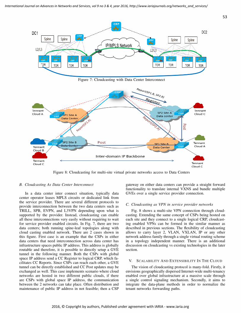
53



Figure 7: Cloudcasting with Data Center Interconnect

Figure 8: Cloudcasting for multi-site virtual private networks access to Data Centers

B. Cloudcasting As Data Center Interconnect

In a data center inter connect situation, typically datacenter operator leases MPLS circuits or dedicated link fromthe service provider. There are several different protocols toprovide interconnection between the two data centers such asTRILL, SPB, EVPN, and L3VPN depending upon what issupported by the provider. Instead, cloudcasting can enableall these interconnections very easily without requiring to waitfor service provider enabled circuits. In Fig. 7, there are twodata centers; both running spine-leaf topologies along withcloud casting enabled network. There are 2 cases shown inthis figure. First case is an example that the CSPs in eitherdata centers that need interconnection across data center hasinfrastructure spaces public IP address. This address is globallyroutable and therefore, it is possible to directly setup a GVEtunnel in the following manner. Both the CSPs with globalspace IP address send a CC Register to logical CRP, which fa-cilitates CC Reports. Since CSPs can reach each other, a GVEtunnel can be directly established and CC Post updates may beexchanged as well. This case implements scenario where cloudnetworks are hosted in two different public clouds, if thereare CSPs with global space IP address, the communicationbetween the 2 networks can take place. Often distribution andmaintenance of public IP address in not feasible; then a CSP

gateway on either data centers can provide a straight forwardfunctionality to translate internal VXNS and bundle multipleGVEs over a single service provider connection.

C. Cloudcasting as VPN in service provider networks

Fig. 8 shows a multi-site VPN connection through cloud-casting. Extending the same concept of CSPs being hosted oneach site and they connect to a single logical CRP, cloudcast-ing enabled VPNs can be formed in the similar manner asdescribed in previous sections. The flexibility of cloudcastingallows to carry layer 2, VLAN, VXLAN, IP or any othernetwork address family through a single virtual routing schemein a topology independent manner. There is an additionaldiscussion on cloudcasting vs existing technologies in the latersection.

V. SCALABILITY AND EXTENSIBILITY IN THE CLOUD

The vision of cloudcasting protocol is many-fold. Firstly, itenvisions geographically dispersed Internet-wide multi-tenancyenabled over global infrastructure at a massive scale througha single control signaling mechanism. Secondly, it aims tointegrate the data-plane methods in order to normalize thetenant networks forwarding paths.

54



Figure 9: Growth in CRP-CSP connections at scale

Figure 10: Hierarchical CRP System

A. Scalability in ControlplaneCloudcasting is a virtual routing scheme for cloud based

environments that maybe hosted across multiple serviceprovider networks or at multiple sites. In the preceding section,it is assumed that the CRP is a single centralized entity.

1) Hierarchical CRP-system: Cloud networks are expectedto be distributed beyond a local site, for example, a tenantnetwork is not scoped with in a single provider domain, butneeds to communicate with entities residing behind multipleprovider domains. Assuming there are millions of such tenants,then a single CRP managing high number of sessions withas many CSPs in the Internet becomes unmanageable with aflat architecture as shown above in Fig. 9. A centralized CRPnode can cause severe performance bottlenecks when servicinglarge number of CCC messages such as Register and Reportsoriginating from high number of CSPs simultaneously.

The ability to scale is the most important requirement forcloudcasting routing scheme, otherwise, it does not providea converged deployable solution. With in the cloudcastingprotocol a distributed and hierarchical system of CRPs isproposed to exchange CRP control plane signaling. The systembuilds a connected graph of CRP instances across serviceprovider domains. In order to create a hierarchy, a CRP nodeis associated with a scope. The scope maybe up to a localsite (CRP-site), provider-specific (CRP-SP) or inter-provider

(CRP-IP). The definition of cloud networks is also extendednow to have scope with in (a) local site, (b) a single provideror (c) multiple providers.

An example of a 3-tier CRP hierarchical system is shownin Fig. 10. In this figure, the CRPs inside the dashed linedbox connected together form a CRP system. A CRP-Site(nodes with IP address 3.1.1.10, 3.1.1.20, 1.1.1.10, 1.1.1.20and 2.1.1.10) is an instance of a local CRP where CSPs froma physical location or a site connect to and is at the lowestlevel node in CRP system hierarchy. A CRP-SP (nodes with IPaddress 30.1.1.1, 10.1.1.1, 20.1.1.1) corresponds to a middle-tier CRP in a provider specific space and has a role of in-terconnecting multiple CRP-Sites in a given region in a singleadministrative domain. Finally, at the highest-tier of CRP hier-archy is a CRP-IP that supports inter-provider communication.The communication between CRP-Site to CRP-SP and CRP-SP to CRP-IP respectively is required to exchange discoveryof cloud networks that are scoped to extend beyond a specificsite, administrative domain respectively. In Fig. 10, it is shownmulti-provider CRPs, CRP-IPs form a cluster together. Eachnode (IP address 300.1.1.1, 200.1.1.1, 100.1.1.1) cluster hasequal status of cloud network Cloudcasting Information Base(CCIB).

2) CC Protocol Extensions: In order to extend cloudcastingsignaling to Hierarchical CRP the following additions to thebase protocol are proposed

• Originating CRP TLV: It identifies the source of aCC Register in a CRP system hierarchy. It is usedmaintain mapping of CRP-Site and cloud networks orVXNs in CRP-SP. In addition, CRP Role Attribute(local, provider, global) is also included to determinethe scope of CRP.

• VXN Scope Attribute: It is used to describe the scopeof a cloud network.

• Cloudcasting Information Base (CCIB): The CCIB isthe control information base maintained at each CRPis aware of the scope of a signaling and originatingsource of the request. It is a stateful table that is learntand looked at upon receiving Register and Reportsfrom neighboring CRPs. Additionally, the CCIB statein each CRP may be stored separately for upstreamand downstream in CRP-SP. A CC Report is generatedand distributed in a similar manner.

3) Single provider scenario: Consider a scenario of singleadministrative domain on the left side of the Fig. 10 CRP-SP (30.1.1.1) and two CRP-Site with IP address 3.1.1.10 and3.1.1.20. Further assume that a cloud network Cn is scoped in asingle provider SP1 (30.1.1.1). As left CRP 3.1.1.10 receives aRegister message from one of connected CSPs, it finds scope tobe provider specific and relays message to CRP-SP (30.1.1.1).Before doing so, TLV extensions as per previous sections areadded. Receiving CRP-SP maintains (3.1.1.10, Cn) mappingin its information base. At a later time if another CRP say3.1.1.20 sends a CC Register for cloud network Cn, CRP-SP,30.1.1.1 generates a CC Report for both CRPs 30.1.1.10 and30.1.1.20. Finally, CSPs receive Register from their respectiveCRPs and can continue with route distribution.

4) Multi-provider scenario: A more elaborate collaborationis required to distribute cloud networks across multiple admin-istrative domains, more so when these domains are geograph-

55



Figure 11: Normalized GVE Data Encapsulation

ically distributed. Therefore, CRP-IP (CRPs for inter providercommunications) are clustered to store identical Cloudcastinginformation base. In this scenario, all CRP-IPS have identicaldatabase of cloud networks that are to be distributed beyondadministrative domains. A CC Register of scope global is sentfrom CRP-Site to CRP-SP to adjoining CRP-IP. The receivingCRP-IP distributed this information to all other CRP-IPs inthe cluster. Each CRP-IP is then responsible for downstreamdistribution of CC-Register to attached CRP-SPs, if and onlyif it has some knowledge in its information base that a CRP-site has interest in same cloud network. For example, letsassume a new global-scoped cloud network Cn is createdby CSP attached to CRP-site 3.1.1.20. This CRP sends CCRegister with extended TLV to its attached CRP-SP, 30.1.1.1,which in turn relays it to its attached CRP-IP, 300.1.1.1 byreplacing originating CRP as itself in the extended TLV. ThisCC Register is distributed everywhere in CRP-IP cluster. Asthis is a new cloud and no instances exist, the request stays inthe cluster. Similarly, at a later time when a CSP attached toCRP-site, 1.1.1.10 generates a CC Register for Cn, it reachesCRP-IP 100.1.1.1, which determines from its information basethat CC Registers need to be sent to 1.1.1.10, does so and alsosend CC Registers to 3.1.1.20. The CC Reports are generatedin exactly the same manner and finally a GVE tunnel isestablished.

B. Extensibility through normalized data plane

The second important aspect of extensibility in cloudcast-ing protocol is related to the normalization of data planeencapsulation. In preceding section, the GVE encapsulationis defined and Fig. 11 further illustrates it to be highlyflexible and scalable. GVE is extensible by virtue of con-necting 2 heterogeneous clouds through the multi-protocolinformation it carries. The figure also illustrates that GVEexpects flexibility in terms of its position in outer header.It maybe carried as layer-2, layer-3 or MPLS payload andis capable of translating multiple encapsulations for exampleIP, MAC, VLAN, VXLAN, NVGRE and so on. The protocolalso allows that an instance of a cloud networks at a site mayuse NVGRE encapsulation and another site of the same cloudmay continue to use VXLAN encapsulation. It is of greatadvantage to migration of connecting 2 islands of a cloudnetwork transparently without changing anything on the localsite except for enabling cloudcasting between the edges orgateways.

Figure 12: 3-Dimensional Policy Framework for Cloudcasting

VI. POLICY FRAMEWORK FOR CLOUD NETWORKS

A smart policy framework can help build simple orches-tration platforms that do not need to excessively interact withthe infrastructure and can also adapt independently to policychanges within the virtual networks. Even in the cloudcastingframework, most traffic within and across the cloud networksis still required to be subjected to forwarding or applicationspecific policies. In this section a brief discussion of a newpolicy model is presented that in general suits better withthe cloud networks. The policies in any network of scalesuch as an enterprise or a campus tend to be fairly diverse,complex and yet quite similar from one tenant to the other. It isdifficult to describe network policies because they are designedand created from a business logic perspective. The businesslogic itself is created centrallly but must be disaggregated andapplied in parts across different network segments. In case ofcloud-centric environments, it is further obscured because nowthe environment is virtualized and physical location agnostic.The state of art of policy framework is far too fragmented [12][13] [14] [15] both in terms of policy description languageand common specifications for policy distribution. There areseveral vendor specific approaches as well open policy frame-works as well. In our view, it is much simpler to break downnetwork policies for cloud networks across three dimensionsto address different aspects. In cloudcasting architecture, weseparate policy-based interfaces as shown in Fig.12 associatingCSP, CRP and the substrate network through 3 different typesof policies and their scope. These are explained as below.

1) Cross-Network Policies: In this case, considerationsare made to propagate rules that permit or disallow trafficacross different cloud networks to the other through policiesor Service Level Agreements (SLAs). These type of policiesinterface at higher level of abstraction. For example, it mayalso be necessary to specify if dev-test clouds can access thedatabase from production clouds. Within cloudcasting, this isan interface between CRP and CSP. It is extremely simpleto associate such policies on CRP, then when the Registerrequest is made, CRP may deny or accept the request to joina certain cloud network. The dotted lines on right-hand sideof the Fig.12 shows the scope of such policies.

2) Inter Cloud Network Policies: It is very common tosetup policies in a network so that traffic must get steeredthrough specific service chains. For example, traffic from aningress port is first subjected to firewall then load balancer

56



and finally to an application server. Such policies are notinfrastructure related and are within a cloud network thatmay need distribution within a site or across multiple sites.Once tenant networks are discovered, CSPs have a path todistribute policies through CSP-CSP policy interface. Thisscope is shown as CSP-CSP through solid line on the bottomright of Fig.12.

3) Tenant to Substrate Network Policies: In section II, itis explained that cloud centric tenant networks borrow andconsume resources from substrate networks and tenants do notown any physical resources themselves. Yet, it is necessary toallocate resources to support quality assurance and bandwidthguarantees. Since tenant network operators cannot reserveresources they do not own and any bulk pre-allocation doesnot align with infrastructure independence, a separate tenant tosubstrate network policy interface is mandatory. This interfaceis not related to cloudcasting and therefore, should not bepart of cloudcasting. However, there is a need for generalizedreservation and administration method, be it a protocol or APIbased that may be used between tenant and substrate networks.This scope is shown on the left-hand side of the Fig.12.

In previous two sections additional features of cloudcastingsuch as extensibility, scalability, normalization and policyinterfaces were briefly explained to demonstrate that cloud-casting framework is entirely viable solution for interconnec-tivity of cloud networks. In this paper, emphasis is on corearchitecture extensions and many details relating to extendedTLVs are omitted out. For the same reason, policy interfacedetails are excluded from the paper.

VII. EVALUATION AND ANALYSIS

The cloudcasting architecture and primitives have beenimplemented in our research laboratory. We have successfullyused the cloudcasting architecture and control protocol toimplement the above mentioned use cases. First and foremost,we emphasize that the cloudcasting architecture represents aparadigm shift. It is a truly converged technology for virtualnetworks, clouds, and VPNs. No matter what the structure ofthe underlying substrate network is, any/all types of virtualtenant networks can be constructed in the same way by usingcloudcasting.

A. Qualitative AnalysisThe Cloudcasting suitability and applicability can only be

verified vis-a-vis characteristics of the cloud-scale environ-ments. Therefore, we have laid importance on the primarycharacteristics of cloud centric networks that are elasticity,efficiency, agility, and distribution. The Cloudcasting controlplane is elastic, because it can grow and shrink independentlyof (1) the heterogeneous protocols of the substrate network,(2) number of virtual network attachment points, the CSPs,(3) number of domains (autonomous systems), (4) number ofroutes within a users virtual network, and (5) mobile nature ofthe host stations. The Cloudcasting control plane is efficient,because (1) no CSP distributes routes to other CSPs that theyare not interested in, (2) thus, no CSP receives and storesroutes of virtual networks of non-interest or the ones it is notconnected to. In addition, the control plane is fully distributedin such a manner that through a single primitive (post-update);change in the tenant networks can be announced immediately,from the spot of change without configuration changes. The

Cloudcasting allows for agile networking. Every time when anew CSP is added, it is only required to configure the newlyadded CSP by using a few lines of commands. Every timewhen a CSP is deleted, no additional configuration changeor for that matter nothing else needs to be done. This isbecause cloudcasting has a built-in auto-discovery mechanismthat has not been seen in the embedded virtual networks.The Cloudcasting data plane scales as well. Its default GVEencapsulation protocol allows to support 256 million clouds.In other technology such as, VXLAN, it only up to 16 millionclouds are supported. Due to the limitation of space, we wontdiscuss and describe other more desirable characteristics.

B. Prototype ImplementationIn our lab, three small-scale data centers were implemented

for the demonstration of functionality. Each data center hada CSP network element and also connected to the CRP incloudcasting enabled network. In addition, each data centeralso comprised of one or two hosts; and each host had at least2 VMs spawned with their own private IP addresses. All thetraffic from VMs or hosts was default forwarded to the CSP,which performed the data plane encapsulation/decapsulationand forwarding between CSPs. One of the data centers servedas media server center and others were clients. The purposeof this setup is to show isolation with in a virtual networkdomain and VM mobility from one data center to the other. Thesetup also has a network management system that provisionsCSPs about virtual networks and VM hosted with in them.The development environment is entirely based on open sourcecode or is in-house developed. The code is implemented in thefollowing categories -

1) CSP control plane software: CSP software is based onquagga (0.99.24) [16] open source, because it provides anideal and quick router/switch like development environmentto use many features such as command line for configuration,message parsing, daemon and process communication featuresthat are already build in quagga. A csp daemon was created inquagga base and new code was written to provide followingfunctions• CSP-CRP Connection: CSPs listen to a TCP port and

connect to CRP, which is a configurable IP address.On this channel Register and Report messages areexchanged.

• CSP-CSP Communication: CSPs listen to anotherTCP port to connect to CSP IP addresses receivedin Report messages. This channel is used for Postupdates for virtual route exchanges. Once the routesare learnt from peer CSPs, the datapath process isupdated.

• CSP Network Management Interface: CSP also in-terfaces with a management entity to receive virtualnetwork specifications or changes thereafter. Thesechanges are pushed as an XML file and can easilybe changes to REST APIs.

2) CSP datapath: CSP data plane is implemented as an-other daemon using pcap library [17] to perform tunnelingfunctions for traffic between hosts and CSPs. It maintains twoforwarding rules passed from CSP control process, viz. host-CSP and CSP-host. Since the aim was proof of concept anddata plane is implemented in software, it is irrelevant to discussthe forwarding path throughput.

57



3) CRP control plane software: While, CSP control anddata plane are developed in C; CRP code is entirely writtenin Java, consequently both Java and C code base for the CCCprotocol exists. CRP uses neo4j [18] based highly scalablegraph databases to store and visualize relationships betweenthe virtual networks and CSPs.

4) Network Management Interface: The management sys-tem is in-house developed software for a network operator.Written using C# as a web application on IPAD, an operatoris able to add or delete new virtual networks to a specific datacenter as well as add, delete and move VMs from one datacenter to the other.

The above code may be made available to those interestingin further research in cloudcasting. Due to lack of testbedsand other resources quantitative comparison has not beenperformed adequately and results are not available yet. It is ourintent to demonstrate controlplane efficiency through analysisof bytes and messages transferred under several approaches.

VIII. RELATED WORK

There are several works available that partially solve net-work virtualization problem; however, they do not provide acomplete and consistent solution that sufficiently fulfills allbasic requirements discussed earlier in this paper. In whatfollows, we discuss and compare a few prominent network-overlay approaches.

A. IETF NVO3The cloudcasting architecture and protocol shares some

goals chartered by the IETF working group NVO3 (NetworkVirtualization Overlays over Layer 3) [19]. The purpose ofNVO3 is to develop a set of protocols and/or protocol exten-sions that enable network virtualization within a data centerenvironment that assumes an IP-based underlay. Cloudcastingvaries from NOV3 in that cloudcasting is not just restrictedto the data center, and it does not expect a specific structureor protocol conventions in the underlay. The control plane ofNVO3 may seem to be a reformulation of the BGP architec-ture, where NVEs (Network Virtualization Edge) and NVA(Network Virtualization Authority) resemble iBGP speakersand Route Reflectors, respectively, and NVO3-VNTP [20]resembles BGP update messages between an iBGP speakerand its Route Reflector. Therefore, NVA needs to learn andstore routes from an NVE and then distribute those routesto other NVEs. In contrast, in Cloudcasting virtual routeinformation is a function between CSPs, the routes are onlydistributed between the CSPs, the CRP is not involved inroutes. CRP is used for cloud membership auto-discoveryand thus enables agile provisioning. Auto-discovery functionsare also missing from NVO3, where are they are natural tocloudcasting protocol. We should emphasize that CRP hasno route database inside that has a significant impact on thesize of the database in CSP. This differentiation is commonwith other related work discussed in the following sections.NVO3 suffers from the existence of multiple encapsulations,the working group has not been able to make progress on anative control plane design and most often resort to EVPNcontrol plane. The group is also divided on the subject ofdata plane format whether the group shall support a singleor multiple encapsulations. In this regard, Cloudcasting GVEsupports multiple types of data plane encapsulations inherentlyas is discussed in earlier extensibility section V (B).

B. VXLAN and EVPNVXLAN is a data plane format for network overlay en-

capsulation and decapsulation, and EVPN has been proposedas the control plane for VXLAN [21] [9] [22]. BGP wasoriginally designed for inter-domain routing across serviceprovider networks. Although, EVPN is the only IETF defineddistributed control plane protocol, BGP in data center networkvirtualization leads to may operational overheads as explainedin the following ways

1) In order to deploy EVPN, the network operator mustconfigure something like an AS (autonomous system)in substrate networks, which is not really a data centerdesign concept. In addition to this many other BGP-VPN related constructs such as route-targets (RT)are route-distinguisher (RD) must be defined. Con-figurations can be templatized to reduce complexity,yet to keep the network consistent these parametersmust be carefully chosen and during network outages,trouble shooting is extremely difficult because anoperator has to be aware of the mappings of RTsand RDs to virtual networks, not to mention thathigher number of configuration parameters adds tomanagement traffic. A sample configuration maybefound at [23].

2) Running BGP in a data center requires VTEPs to beiBGP speakers. This can also lead to serious scal-ability problems of a full-mesh of peering sessionsbetween iBGP speakers (VTEP-BGP). Typically, toaddress this problem, deployment of Route Reflectors(RR) is recommended. RRs then speaks with everyother VTEP-BGP to synchronize their BGP-RIB. Asa result, no matter if a VTEP needs a route or not,all the other VTEPs will always send their routes tothe VTEP through a Route Reflector, and the VTEP isrequired to filter out not needed routes through RouteTarget and other BGP policies. Distribution of notneeded virtual routes from RR to VTEP-BGP leviesan unnecessary overhead on the substrate network andburn CPU power, processing these BGP messages.

3) BGP in the data centers not only makes operationalcost of data centers as high as that of a serviceproviders network it also lacks the agility becauseBGP heavily relies on configurations (it is well knownthat configuration errors are a major cause of systemfailures [8]). For example, when a new BGP-VTEPis added/removed the operator has to configure allthe BGP peering relationships by stating which BGPneighbors are peering among each other.

Observe that when BGP was first designed, some distributionand peering principles were built-in; for example, iBGP peersshould have received and synchronized the same copies ofroutes. In the case of clouds, many such principles are notapplicable and exceptions need to be added to BGP protocolto address requirements for the cloud networks. Cloudcastingarchitecture does not suffer from the drawbacks describedabove. By means of auto-discovery and route distribution, onlyspecific routes of a virtual network are distributed. Moreover,the role of CRP does not require it to be an intermediatehop between two CSPs to distribute the routes. The detailedcomparison and evaluation is still in progress and will bepublished at a later stage.

58



C. LISP based data center virtualizationAlthough Locator ID Separation Protocol (LISP) [11] is

not an inherent data center virtualization technology, it has aframework to support network overlays. LISP achieves this bydistributing encapsulated tenant (customer) routing informationand traffic over provider (substrate) network through its controlplane based on a mapping system. The LISP architectureincludes Ingress/Egress Tunnel Routers (xTRs) and a mappingsystem (MS/MR) that maintains mappings from LISP EndpointIdentifiers (EIDs) to Routing Locators (RLOCs). LISP requiresmapping information to be pulled on-demand and data-driven,xTRs also implement a caching and aging mechanism for localcopies of mapping information. Cloudcasting CSPs and LISPxTRs are similar in that they are the virtualization tunnelendpoints performing encapsulation and decapsulation. Butthe VXN route database and LISP’s mapping databases aredifferent as below

1) LISPs mapping system [24] is a separate proto-col element and is based on hierarchical design ofDomain Name Server (DNS). The xTRs work incollaboration with mapping server (MS) and mapresolvers (MR). First and foremost, an xTR mustregister its EIDs with the mapping system. When aremote xTR is ready to exchange data for an EID,it will query mapping system to find the xTR whereEID is located, create the local mapping cache (isreferred to as pull method) where entries are agedwhen not needed. In comparison, CSPs are able todiscover each other on the basis of VXN, withoutregistering any EIDs with CRP. Once CSPs and VXNmappings are formed vFIBs are built by post updates.Thus, routes are local and significant only to the CSP.

2) An xTRs local database is built on demand afterreceiving a data packet without knowing its mappinginformation, which may expose sender to securityrisks because the destination is unknown, while CSPsVXN CCIB is signaled through the cloudcastingcontrol protocol over an authorized communicationchannel. The infrastructure can flexibly make thechannel as secure as it prefers using security andencryption protocols.

3) A CSP can auto-discover other CSPs that join thesame VXNs, while LISP xTR can only know aboutanother particular xTR after querying the mappingdatabase.

IX. VIRTUALIZATION IN MOBILE NETWORKS USINGCLOUDCASTING

During our research and study of policy based constraintsin Cloudcasting, we came across Fifth Generation (5G) net-work slices. We concurred with the authors of Next GenerationMobile Networks (NGMN) [25] white paper that 5G networkswill be a collection of service aware logical networks. It wasobvious that a higher degree of automation is vital in 5G forservices to be discovered, provisioned and resources to be ap-portioned/released. Authors have discussed using Cloudcastingas fundamental block in [26] for auto-discovery of services inmobile network supporting cloud hosted environments. In thiswork, a network slice corresponds to a VXN in cloudcasting,while service extensions (resource specifications) are newlyadded and associated with a network slice. The main idea

in this paper deviates from symmetric VXN relationship ofCloudcasting. 5G services in [26] have asymmetric producerand consumer association. First, network segments participatein cloudcasting system and network slices are bound to thosesegments. Then in a producer role, the services announcethemselves, their location in the system and their resourcerequirements. Thus services become available and discoverablewith in those slices. Subsequently, in the consumer role, anend user or device attaches itself to the service; networkresources are allocated across different network segments. Theprocedures just described are done dynamically that allows amobile network system to be easily managed. The idea of auto-discovery is fairly advanced and prototyping of this approachis still being done.

X. FUTURE WORK

In this paper, we have presented several extensions toCloudcasting protocol in terms of policy, services and scal-ability that makes it more complete. Cloudcasting can bethought of as a generalized virtual routing framework. Itsvalidity, scalability and extensibility as a single mechanismfor implementing cloud centric networks. There are severalscenarios not explored yet include containers, microservicesand SD-WAN.

Since the publishing of original paper, we have designedan integrated policy model as the basis of interface betweensubstrate and virtual network. The model allows distributionof tenant policies using the base protocol. However, resourceallocations over substrate network were not found to be assimple and in fact led to new work as an extension tocloudcasting protocol. The corresponding data structures andprototype implementation are an open for further research atthe time of writing this paper.

Previous section alluded to Cloudcasting extensions forservice distribution in mobile networks. The 5G networkslice definition is still evolving, therefore, an opportunity liesin exploring this topic further both from prototyping andvalidation perspective. Finally, although the prototype for baseprotocol is available, further comparison study, assessment ofcontrol plane signaling overheads, robustness and datapath op-timizations related work is not complete yet and we welcomecontributions from interested research community.

XI. CONCLUSION

Cloud-scale networking environments require a technologywhere virtual networks are first class objects; such that thecoarse policies and routing decisions can be defined andapplied on the virtual networks. Cloudcasting is a routingsystem based on converged, unified network virtualization andwill evolve better because of lower provisioning costs andenhanced agility through auto discovery. This paper presentedseveral new concepts; it extended original idea from singledata center to explain global scale distribution of VXNsacross multiple providers, sites and domains. Many use casesare further discussed in great detail. We also shared ourperspective on policy model, which plays an important rolein interaction between virtual and physical infrastructures toprovide operation and management functions. The prototypeimplementation is discussed at great length and interestedreaders are encouraged to contact the authors for code. As aninteresting application, we have taken the idea of cloudcasting

59



for virtual networks and extended it to the auto-discovery ofservices in the 5G network slicing context that further bolstersadaptability and flexibility of the framework.

ACKNOWLEDGMENT

The authors are thankful to the members of the Cloud-casting project, particularly those involved in the early designand proof of concept and prototype development for theircollaboration and fruitful discussions.

REFERENCES

[1] K. Makhijani, R. Li, and L. Han, “Cloudcasting: A New Architecturefor Cloud Centric Networks,” in Proc. IARIA Int. Conf. on Comm.Theory, Rel., and Qual. of Serv. (CTRQ), Lisbon, Portugal, February2016.

[2] D. Fedyk, P. Ashwood-Smith, Allan, A. Bragg and P. Unbehagen, “IS-ISExtensions Supporting IEEE 802.1aq Shortest Path Bridging,” InternetEngineering Task Force (IETF), April 2012.

[3] IEEE, “IEEE Standard for Local and metropolitan area networksMe-dia Access Control (MAC) Bridges and Virtual Bridged Local AreaNetworksAmendment 20: Shortest Path Bridging,” June 2012.

[4] D. Eastlake, T. Senevirathne, A. Ghanwani, D. Dutt and A. Banerjee,“Transparent Interconnection Of Lots Of Links (Trill) Use Of Is-Is,”Internet Engineering Task Force (IETF), April 2014.

[5] M. Sridharan et al., “Virtual eXtensible Local Area Network (VXLAN):A Framework for Overlaying Virtualized Layer 2 Networks over Layer3 Networks,” Aug. 2014.

[6] M. Mahalingam et al., “NVGRE: Network Virtualization using GenericRouting Encapsulation, draft-sridharan-virtualization-nvgre-08 (work inprogress),” Internet Engineering Task Force (IETF), 2015, pp. 1–10.

[7] J. Gross, T. Sridhar et al., “Geneve: Generic Network Virtualization En-capsulation, draft-ietf-nvo3-geneve-0,” Internet Engineering Task Force(IETF), April 2015.

[8] T. Xu, Y. Zhou, “Systems approaches to tackling configuration errors: Asurvey, article no.: 70, acm computing surveys (csur) volume 47 issue4,” July 2015.

[9] A. Sajassi et al., “A Network Virtualization Overlay Solution usingEVPN,” Internet Engineering Task Force (IETF), February 2015.

[10] M. Yu, Y. Yi, J. Rexford, and M. Chiang, “Rethinking virtual networkembedding Substrate support for path splitting and migration,ComputerCommunication Review,” vol. 38, 2008 2008, pp. 17–29.

[11] D. Farinacci, V. Fuller, D. Meyer, and D. Lewis, “The Locator/IDSeparation Protocol (LISP),” Internet Engineering Task Force (IETF),January 2013.

[12] VMWare Micro segmentation. web:https://www.vmware.com/content/dam/digitalmarketing/vmware/en/pdf/products/nsx/vmware-microsegmentation-solution-overview.pdf. (2015)

[13] Simplified Use of Policy Abstractions (SUPA). web:https://datatracker.ietf.org/wg/supa/charter/. (2015)

[14] Opendaylight, Group based Policy. web:https://wiki.opendaylight.org/view/Group Based Policy (GBP). (2015)

[15] Cisco Application Centric Infrastructure(ACI). http://www.cisco.com/c/en/us/solutions/data-center-virtualization/application-centric-infrastructure/index.html. (2015)

[16] Quagga Routing Software Suite, GPL licensed. http://download.savannah.gnu.org/releases/quagga/quagga-0.99.24.tar.xz.

[17] libpcap, a portable C/C++ library for network traffic capture. http://www.tcpdump.org/.

[18] Neo4j, a highly scalable native graph database. https://neo4j.com/.[19] M. Lasserre et al., “Framework for Data Center (DC) Network Virtu-

alization,” Internet Engineering Task Force (IETF), October 2014.[20] Z. Gu, “Virtual Network Transport Protocol (VNTP),” Internet Engi-

neering Task Force (IETF), October 2015.[21] E. Rosen and Y. Rekhter, “BGP/MPLS IP Virtual Private Networks

(VPNs),” Internet Engineering Task Force (IETF), April 2006.[22] Sami et al., “VXLAN DCI Using EVPN, draft-boutros-bess-vxlan-evpn-

01.txt,” Internet Engineering Task Force (IETF), January 2016.

[23] VXLAN Network with MP-BGP EVPN Control Plane DesignGuide. http://www.cisco.com/c/en/us/products/collateral/switches/nexus-9000-series-switches/guide-c07-734107.html. [retrieved: April,2016]

[24] V. Fuller et al. LISP-DDT: LISP Delegated Database Tree, Workin Progress. https://tools.ietf.org/html/draft-ietf-lisp-ddt-08. [retrieved:September, 2015]

[25] N. Alliance, “NGMN 5G White Paper,” White paper, February 2015,pp. 1–125.

[26] K. Makhijani, S. Talarico, and P. Esnault. Efficient Service Auto-Discovery for Next Generation Network Slicing Architecture, presentedat O4SDI, IEEE NFV-SDN 2016. Unpublished.

60



Device Quality Management for IoT Service Providersby Tracking Uncoordinated Operating History

Megumi Shibuya†, Teruyuki Hasegawa† and Hirozumi Yamaguchi‡†KDDI Research, Inc. ‡Osaka University

Saitama, JAPAN Osaka, JAPAN e-mail: {shibuya, teru}@kddi-research.jp e-mail: [email protected]

Abstract—According to the widespread of Internet of Things(IoT) services with a huge number of IoT devices, service providers will face the challenges how to grasp the product quality of the IoT devices by themselves in order to make IoT services highly reliable and dependable. The cumulative failure rate is an important reliability index for evaluating the product quality and service reliability of IoT devices. However, in the horizontal specialization business model, IoT service infrastructure is often operated by multiple players such as service providers and device vendors, and device management information that is necessary to obtain the cumulative failure rate is independently and uncoordinatedly owned by them. In this paper, we propose a method of calculating the cumulative failure rate in such environment. We design an algorithm to aggregate and organize such distributed, uncoordinated information to derive the device operating history, which is fed into the cumulative failure rate calculation formula. Through several simulation experiments, we show the effectiveness of our method in several realistic scenarios, where we also arrange several uncoordinated cases.

Keywords - IoT; Service eliability; Cumulative failure rate;Operating history; Multiple players; Horizontal specialization business model

I. INTRODUCTION

Recently, the concept of Internet of Things (IoT) has been widely penetrating into our daily lives and IoT device reliability is one of fundamental, technical issues to achieve IoT-enabled world. We have been focusing on such IoT device reliability in reference [1] and this issue enhances the concept of IoT device reliability management for more realistic cases.

According to [2], the number of devices which are available for mobile access is expected to grow toapproximately 50 billion units (6.58 units per user) by 2020.In IoT enabled systems, a huge number of IoT devices are being interconnected, and such infrastructure becomes more sophisticated and smarter to support our lives.Simultaneously, as it becomes more indispensable, it should be more reliable to achieve sufficient service availability [3]-[5]. This cannot be achieved without high reliability and dependability of IoT devices themselves.

In the research field of reliability engineering, there are several kinds of reliability-indexes such as Mean Time Between Failure (MTBF), Mean Time To Repair (MTTR), Mean Time To Failure (MTTF) and Failure in Time (FIT)[6]. In addition, cumulative failure rate is often utilized as a

device reliability index [7]. It is a probability of failureoccurrence in a certain time period starting from the time when the device becomes in operation. The cumulative failure rate is usually derived using the failure rate for every unit of time, which is defined as a ratio of the number of failed devices to the number of devices being in operation in the unit of time. Here, the devices being in operation may vary at every moment not only due to device failure but also due to operational activities such as new device installation, removal and replacement. Therefore, we need to trace the operating history of each device to calculate accurate cumulative failure rate.

However, in order to obtain the operating history of each device, it is required to obtain the dates of device-associated events such as installation of the device, suspension and resumption of device utilization and failure. If the device manufacturers, simply called vendors, themselves provideservices (this way of service provision is called vertically integrated business model [8]), such information can be obtained easily as everything is managed at a single place. In contrast, in horizontal specialization business model [9]-[11]where service providers (simply called providers) purchase the devices from vendors and use them (this style is often seen in smart meter services and the Internet access services), device operating history is owned and managed partially and uncoordinatedly by multiple business operators called players. Furthermore, by changing business environment around the providers, e.g., the number of IoT devices is dramatically increased and demand for service reliability becomes much more severe, we believe each provider itself is required to expand the quality management of devices which the vendors have been dealing with and responsible for. Accordingly, the possibility of lack of information from the perspective of providers is newly exposed. Therefore, the horizontal specialization business model will causes a significant issue in building a single, consistent view of operating history.

We introduce an example case to explain how and why such a situation is seen in the horizontal specialization business model in the following. In smart meter services, an electric company (i.e., a provider) purchases power meters in bulk from a vendor, lends them to subscribers, and stocks the rest as spares. When a power meter becomes out of order, the provider supports to replace it. Since the provider entrusts the repair service to the vendor, the vendor receives the failed power meter directory from a user and repairs it in order to mitigate the provider’s tasks. Then, the vendor is

61



able to manage the product-related information such as theproduction date and the model number of the meter as well as the failure-related information such as the date and reason of failure and the repair process. However, the device operating status (e.g., operating start date) is not observed by the vendor. Meanwhile, the provider has to manage the subscriber information including the asset information (e.g.,the current meter location). Hence, it is not necessary to trace back the information about failure and others. Consequently, in order to obtain a consistent history of meters, it is necessary to design a method of aggregating the management information that are separately and uncoordinatedly managed by multiple players to enable calculation of the cumulative failure rates.

In this paper, we propose a method of calculating the cumulative failure rate, which is an important reliability index that represents device reliability. We assume that services are provided (i) using a large quantity ofhomogeneous devices and (ii) following the horizontal specialization business model where multiple players are involved and management information are owned separately and uncoordinatedly by them. Then, the method aggregates and analyzes those distributed information to derive the operating history of each IoT device to enable the calculation of cumulative failure rates.

The contributions of this work are four-fold.We deal with a significant issue of IoT device management inspired by our business experience on how we grasp and measure the device reliability,which is mandatory to maintain the quality of large-scale IoT service infrastructure operated by multiple players in the horizontal specialization businessmodel.We propose a method to obtain the operatinghistory of each IoT device from various types ofmanagement information. We would like to emphasize that calculating the cumulative failure rate using complete device history is normally done in device management, but taking into account those devices that are often replaced, repaired and reused at different times and locations is not straightforward.We present the experimental result of measuring the accuracy of cumulative failure rates with realistic scenarios where a part of the information is missing.Such a situation often occurs in the real environment.To prove wide applicability of our proposed method,we further evaluate the additional but promising uncoordinated case in which additional information elements are added from the middle, i.e., after the service was launched, due to emerging new operational requirements.

This paper is organized as follows. Section II summarizes related work and Section III introduces a service scenario in IoT infrastructure with multiple players. Section IV presents our method and experimental results are shown in Section V. Section VI considers the additional

uncoordinated case in which some information elements are added after the service launch. Finally, we conclude this work in Section VII.

II. RELATED WORK

There have been various activities on evaluating product quality and device reliability [6][7][12]-[19] including the research field of reliability engineering [6][7]. Several studies on Operation And Management (OAM) issues of IoT devices in IoT service infrastructure [20]-[27]have also been conducted.

As the reliability terms, based on the methods and procedures for lifecycle predictions for a product, there are several kinds of reliability indexes [6]. Mean Time Between Failure (MTBF) is a reliability term in which the average time form the up time after the repair following a failure to the next failure. Mean Time To Failure (MTTF) is that the average length of time before failure of a device. While MTBF is used for repairable device, MTTF is used for non-repairable device. Mean Time To Repair (MTTR) is the termthat the average length of time to repair a failed item.Furthermore, Failure in Time (FIT) reports the number of expected failure per one billion hours of operation for a device. Moreover, cumulative failure rate is often utilized as a device reliability index [7]. It is a probability of failureoccurrence in a certain time period starting from the time when the device becomes in operation. The cumulative failure rate is usually derived using the failure rate for every unit of time, which is defined as a ratio of the number of failed devices to the number of devices being in operation in the unit of time.

References [12]-[14] present evaluation methods at the design or production phase of devices, where the cumulative failure rate is estimated by modeling the occurrence of major failures at the component level of devices. Reference [12]focuses on how to calculate the failure rate of N-channel Metal Oxide Semiconductor (NMOS) devices under Hot Carrier Injection (HCI) mechanism and Time Dependence Dielectric Breakdown (TDDB) failure mechanism. The failure rate models and hypothesis test are proposed for each HCI and TDDB. Reference [13] discusses how to determine a new parameter from failure factors observed in the field, e.g., electrostatic discharge inrush current, to integrate it into a conventional estimation method for more accuratecumulative failure rate at the product design phase.Reference [14] proposes how to use the failure statistics toobtain the failure rate of a particular component according to its real conditions. It also demonstrates how the proposed methodologies are applied for failure rate estimation of power circuit breakers. The methodologies can be used for condition-based reliability analysis for electric power networks, in order to obtain an optimized maintenance strategy. Reference [15] proposes an approach to estimatingthe failure rate for Time-varying Failure Rate (TFR) of the relay protection device with the field data using random failure and aging failure. These approaches assume that all information elements, which are necessary for calculating also the cumulative failure rate, are maintained by the vendor

62



manufacturing the devices, and it is not considered that the number of devices varies by factors other than failures.

The bathtub curve is a common feature of product failure behavior [16]. It is a lifetime of a population of products using a graphical representation. The typical bathtub curve has three phases. The first part is the birth-in period, which is characterized by a high and rapidly decreasing failure rate.The second part is the useful period, when the failure rate remains almost constant. The third part has an increasing failure rate, known as the wear-out period. The bathtub curve can be useful for predicting the device failure if the age of each device is known, however only the characterizations are known.

Reference [17] proposes a one line prognostic algorithm for the power module devices using the operating history of the device to detect the time of failure quickly during operation. Reference [18] proposes the calculating probability of failure using an equipment age model that is relaxed the independence assumption of individual measurements of usage intensity and operating conditions.Moreover, it shows practitioners how to develop a more complete maintenance strategy that allows for bothcorrective maintenance (CM) and condition-based maintenance model (CBM) using the simple decision routine.

On the other hand, in the telecommunication network, it is difficult to calculate the failure rate accurately by reliability engineering methods because the failure rate is calculated by the number of devices and time differentiation of the cumulative number of failure devices at the given timing of elapsed time. References [19][20] propose evaluation methods for product reliability based on the observation of each device’s operation history considering device changes due to non-failure, which is not taken into account in the existing work [7][21]. In reference [19], the instantaneous failure rate of a repairable device for the communication network is calculated as the limit of the average failure rate that is available for the increase and decrease of the number of devices. Namely, the number of cumulative failure rate and the number of devices are estimated as the continuing functions to times. In contrast in[20], they study the applicable condition of the mathematical model for the proposed method.

All the above assume a vertical integration structure in which all the information elements for calculating the cumulative failure rate (or a similar index) are maintained by only one player. In contrast, we are focusing on IoT service infrastructure in which multiple players (e.g., providers and vendors) are collaboratively involved. In such a horizontal specialization structure, which is expected to penetrate the IoT market in the future [11], the followings should be done to manage the product reliability of IoT devices for realizing dependable infrastructure; 1) coordinating the management information provided by each player, 2) extracting and deriving information elements and 3) reconstructing the device operation history from the information elements. Asfar as we know, this is the first activity focusing on IoT device management with multi-player issues.

Meanwhile, there have been many approaches so far toward IoT device applications [22]-[27], which basically

focus on the management and configuration of remote sensor devices over the Internet. For example, Ref. [22] implements IPv6 over 6LoWPAN and RPL and provides CoAP-based control to facilitate sensor device management over the Internet. Reference [23] also takes a remote-management approach where MQ Telemetry Transport is utilized for IoT application and management. In Reference [24], the authors discuss the necessity of wireless sensor network management in a unified manner. They consider that the industrial authorities should be able to provide a network infrastructure supporting various WSN applications and services to facilitate the management of sensor devices, and industrial ecosystem and industrial device management standards have been introduced. Reference [26] is rather unique in the sense that a distributed approach is introduced for IoT device management from a social network point of view, where a social network theory is applied to model the services. Reference [27] discusses cloud-resource management for multi-agent IoT systems, which is also important for entire system coordination. However, they basically focus on the protocol and architecture issues and do not deal with the IoT device management processes and operations.

III. SERVICE SCENARIO

In this paper, we assume IoT infrastructure with multiple players in the horizontal specialization business model.Under this assumption, we explain the device operating and management information that are separately and uncoordinatedly managed by multiple players. The scenariois based on our own experience, so cases hereafter are likely to be seen in the real world business.

As explained briefly in Section I, we target a service provider such as an electric company or a network providerthat purchases the devices in bulk from an IoT device vendorand lends them to subscribers (users). If the IoT device fails, the provider lends an alternative IoT device that is stocked in their warehouse to the subscriber. After receiving it, the user sends the failed IoT device to vendor. As the provider service, it is a common business model that the user lends the device from the provider, such as STB [28].

Figure 1 illustrates the interactions between each player and user. We explain the service provision scenario using this figure.

(1) IoT Device Purchase and Stocking:

The provider purchases IoT devices from the vendor and stocks them as spares. Lending an IoT device from the provider to a user and returning it by the user due to cancellation is conducted via the provider’s warehouse. The provider records the current location of the purchased IoT devices in asset management information. The vendorrecords the product-related information such as the shipping date and model number of IoT devices in shipment management information.

(2) Service Startup:

The provider creates the contract-related information for every user and manages it. The provider lends an IoT device

63



to a user, starts the service and records the service start date in user contract information.

(3) IoT Device Failure and Replacement:

When an IoT device fails at a user location, the user contacts the provider to tell his/her device has been failed.The provider sends an alternative IoT device from their warehouse to the subscriber. After receiving it, the user sends it back to the vendor directly using a preprinted address label included with the alternative IoT device foroptimizing the physical transport route. The vendor repairs the failed IoT device and records the failure-related information such as date and model number (or send-back date or receiving date as the date of failure). After the repaired IoT device is sent from the vendor to the provider, it is stocked in the warehouse. The provider updates the records related to these two devices (i.e., the current locations of failed and alternative devices). The vendorrecords the user’s location ID from the address label as the evidence for the provider to check whether the user returnsthe failed IoT device.

(4) Service Cancellation:

When a user cancels its contract, he/she returns his/herIoT device to the provider. The provider re-stocks it in the warehouse and updates the current location information of the IoT device. Furthermore, the service end date of this user is recorded in the contract-related information.

Figure 1. Interaction among multiple players and user.

In summary, the provider maintains a) contract information with users and b) asset management information of IoT devices, the vendor maintains c) shipment-related information of IoT devices and d) the failure-related information. Here, b) is usually sufficient for asset management by the provider. This is because the provider does not care about whether an IoT device was installed at different locations in the past.

On the other hand, as described in Section I, it is required to obtain the occurrence dates of device-associated events such as installation of the device, suspension and resumptionof device utilization and failure to calculate the cumulative information such as the service start date and suspension and resumption of the device date in this scenario, and the provider does not observe the information such as the failure date. Therefore, each player cannot collect and buildcomplete device-associated information. This is our motivation to provide a method to build complete operatinghistory of each IoT device from such partial, distributed operating and management information as indicated by the above a) to d).

TABLE I. SERVICE OPERATING AND MANAGEMENT DATA

LIST-A) CURRENT DEVICE LIST(MANAGED BY PROVIDER)

List created date (=Today) (Tc) : 2016/09/01

Location (L)

Service start date (T1)

Current device (SN)

Operating start date of current device at L (T4)

1 2016/01/01 a -

3 2016/05/01 b -

4 2016/03/01 c -

: : : :

LIST-B) FAILED DEVICE LIST (MANAGED BY VENDOR)

Location (L)

Failed date (T2)

Failed device(SN)

Operating start date of failed device at L (T5)

1 2016/02/01 a -

3 2016/04/01 a -

1 2016/04/01 b -

: : : :

LIST-C) RETURN DEVICE LIST(OUT OF MANAGEMENT BY PROVIDER)

Location(L)

Return date (T3)

Return device(SN)

Operating start date of return device at L (T6)

3 2016/03/01 c -

5 2016/06/01 d -

2 2016/07/01 e -

: : : :

( : unknown )

Provider

(1) Purchasing and StockingIoT Devices

(3) IoT Device Failure and Replacement

(4) Service cancellation

d) Failure management Info. b) Device current location Info.

Vendor Provider User

Provider User

: IoT devices

Provider User

(2) Service Startup

a) User contract Info.b) Device current location Info.

b) Device current location Info.c) Shipment Info.

Vendor

a) User contract Info.b) Device current location Info.

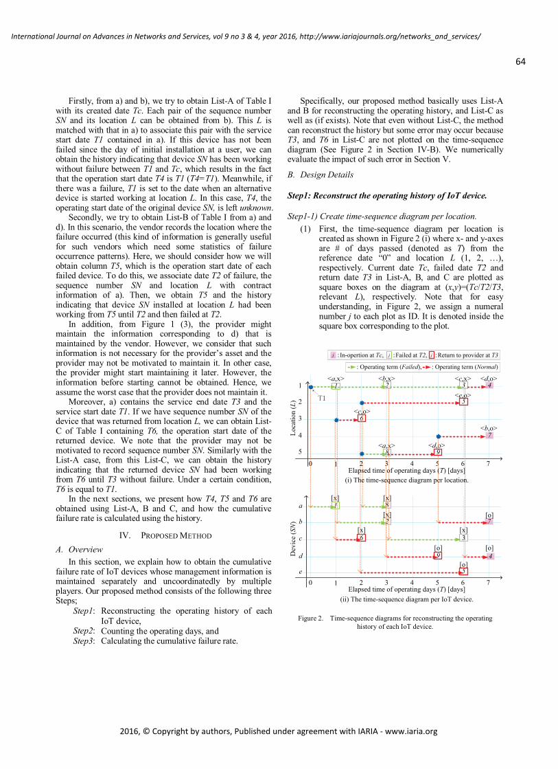
64



Firstly, from a) and b), we try to obtain List-A of Table Iwith its created date Tc. Each pair of the sequence number SN and its location L can be obtained from b). This L is matched with that in a) to associate this pair with the service start date T1 contained in a). If this device has not been failed since the day of initial installation at a user, we can obtain the history indicating that device SN has been working without failure between T1 and Tc, which results in the fact that the operation start date T4 is T1 (T4=T1). Meanwhile, if there was a failure, T1 is set to the date when an alternative device is started working at location L. In this case, T4, the operating start date of the original device SN, is left unknown.

Secondly, we try to obtain List-B of Table I from a) and d). In this scenario, the vendor records the location where the failure occurred (this kind of information is generally useful for such vendors which need some statistics of failure occurrence patterns). Here, we should consider how we will obtain column T5, which is the operation start date of each failed device. To do this, we associate date T2 of failure, the sequence number SN and location L with contract information of a). Then, we obtain T5 and the history indicating that device SN installed at location L had been working from T5 until T2 and then failed at T2.

In addition, from Figure 1 (3), the provider might maintain the information corresponding to d) that is maintained by the vendor. However, we consider that such information is not necessary for the provider’s asset and the provider may not be motivated to maintain it. In other case, the provider might start maintaining it later. However, the information before starting cannot be obtained. Hence, we assume the worst case that the provider does not maintain it.

Moreover, a) contains the service end date T3 and the service start date T1. If we have sequence number SN of the device that was returned from location L, we can obtain List-C of Table I containing T6, the operation start date of the returned device. We note that the provider may not be motivated to record sequence number SN. Similarly with the List-A case, from this List-C, we can obtain the history indicating that the returned device SN had been working from T6 until T3 without failure. Under a certain condition, T6 is equal to T1.

In the next sections, we present how T4, T5 and T6 are obtained using List-A, B and C, and how the cumulative failure rate is calculated using the history.

IV. PROPOSED METHOD

A. Overview In this section, we explain how to obtain the cumulative

failure rate of IoT devices whose management information is maintained separately and uncoordinatedly by multiple players. Our proposed method consists of the following threeSteps;

Step1: Reconstructing the operating history of each IoT device,

Step2: Counting the operating days, andStep3: Calculating the cumulative failure rate.

Specifically, our proposed method basically uses List-Aand B for reconstructing the operating history, and List-C as well as (if exists). Note that even without List-C, the method can reconstruct the history but some error may occur because T3, and T6 in List-C are not plotted on the time-sequence diagram (See Figure 2 in Section IV-B). We numerically evaluate the impact of such error in Section V.

B. Design Details

Step1: Reconstruct the operating history of IoT device.

Step1-1) Create time-sequence diagram per location.(1) First, the time-sequence diagram per location is

created as shown in Figure 2 (i) where x- and y-axes are # of days passed (denoted as T) from the reference date “0” and location L (1, 2, …), respectively. Current date Tc, failed date T2 and return date T3 in List-A, B, and C are plotted as square boxes on the diagram at (x,y)=(Tc/T2/T3,relevant L), respectively. Note that for easy understanding, in Figure 2, we assign a numeral number j to each plot as ID. It is denoted inside the square box corresponding to the plot.

Figure 2. Time-sequence diagrams for reconstructing the operating history of each IoT device.

1 2 3

8

6

4

7

1

2

3

4

<a,x>

<c,o>

<d,o>

<e,o>

<d,o>

<b,o>

<b,x>

<a,x>

<c,x>

1

3

2

6

9

7

4

a

b

c

d

e

[x] [x]

[x]

[x][x]

[o]

8

0 1 2 3 4 5 6 7

0 1 2 3 4 5 6 7

(ii) The time-sequence diagram per IoT device.

(i) The time-sequence diagram per location.

[o]

[o]

9

Elapsed time of operating days (T) [days]

Elapsed time of operating days (T) [days]

Dev

ice

(SN

)Lo

catio

n(L

)

5

j j jIn-opertion at Tc, Failed at T2, Return to provider at T3

: Operating term (Failed), : Operating term (Normal)

5

5[o]

65



(2) For each plot j, device SN and device operating status x=”Failed” or o=”Normal” at the relevant date are associated as its attribute. For instance in Figure 2 (i), plot j=8 with <a,x> (at T=3 and L=5) means that the device a was “Failed” at location L=5 (then it was sent back to the vendor for repair). Plot j=7 with <b,o> means that the device b was“Normal” at L=4 (therefore, it is in-operation now (T=7)). Plot j=9 with <d,o> means that the device dwas “Normal” at L=5 (because it was returned to the provider without failure due to user cancellation at T=5).

(3) Service start date T1 at location L in List-A is plotted on the diagram.

(4) We assume that the failed device is replaced to another device on the same day for non-stop service. Along the time-sequence of each location L, the plots on it are traced back from the current date Tc(T=7) to the reference date (T=0) in order to determine the start date (referred to as Sj) of each plot j at the location. The date of j’s previous plot is regarded as the start date of j. For example, the start date of device b at plot j=2 ((x,y)=(3,1)) is determined as S2=1 because its previous plot (j=1) is at T=1 ((x,y)=(1,1)).

(5) The operating term for each plot j can be extracted as the term from Sj to T of plot j. For example, device b at plot j=2 is operated from S2=1 to T=3 sothe term is 2 days. As another example, device b at j=7 ((x,y)=(7,4)) is operated from S7=5 to T=7 (now in-operation) so the term is also 2 days.

Step1-2) Transform time-sequence diagram per location to per IoT device.

(1) The time-sequence diagram per IoT device (see Figure 2 (ii)) is transformed from Figure 2 (i). At first, each plot j in Figure 2 (i) is re-plotted on Figure 2 (ii) according to the device SN in its attribute. Note that the device operating status x/o in its attribute is inherited. For instance, plot j=2 with <b,x> ((x,y)=(3,1)) in Figure 2 (i) is re-plotted to j=2 with [x] ((x,y)=(3,b)) in Figure 2 (ii).

(2) For each plot j, the relevant operating term from Sjto T of the plot j is drawn on Figure 2 (ii). It is easy to obtain each IoT device’s operating history by collecting operating terms per device from Figure 2(ii). For instance, the operating history of device bincludes two operating terms, i.e., S2=1 to T=3 (Failed) and S7=5 to T=7 (Normal).

Step2: Counting the operating days.Two types of operating days are counted per IoT device

from the operation histories. The first type is referred as “Failed days” (P) which is ended with a plot derived from T2, i.e., failed date. The second type is referred to as “Normal days” (Q) which is ended with a plot derived from T3 or Tc, i.e., return or current date without failure. For counting the operating days of each IoT device, an operation

term of the device is selected in chronological order and checked whether the term is ended by T3 or not. If so, the term should be concatenated to the next operating term (if any) as a single piece of operating days. For example in Figure 2 (ii), the device b is set P=2 and Q=2, while the device c is set P=4(=1+3), and the device d is set Q=3(=2+1). P and Q of each device are shown in Table II.

TABLE II. THE OPERATING DAYS FOR EACH SN IN FIGURE 2 (ii)

SN # of operating days(# of terms)

Operating days [days]1st 2nd

a 2 (2) P=1 P=1

b 2 (2) P=2 Q=2

c 1 (2) P=4(=1+3) -

d 1 (2) Q=3(=2+1) -

e 1 (1) Q=4 -

Step3: Calculating the cumulative failure rate.From both Failure days and Normal days in Step2, the

cumulative failure rate is calculated. Let f(x) denote the failure density function, the failure occurrence probability until time i has passed, i.e., the cumulative failure ratio F(i),is expressed in equation (1) [6].

( ) = ( ) We can approximately obtain the following difference

equation by differentiating equation (1) and substituting infinitesimal di to the unit time (a day).( ) ( 1) = ( )

Here, let ( ) denote the failure rate of i-th unit time.Since f(i) is expressed as( ) = 1 ( 1) ( ) we can obtain the following equation:( ) = ( 1) + 1 ( 1) ( ), where (0) = 0, ( ) ( )( ) ( ) ( = 1, 2, … ). Note that n(i) and N(i) are the number of failed devices (P = i-1) at day i, and the number of in-operation devices at the end of day i, respectively. From the above discussions, the cumulative failure rate can be calculated from the operating history.

66



In addition, m(i) denotes the number of returned devices,which is suspended at day i, is given by the following equation: ( ) = ( 1) ( ) + ( ) Assuming that ( ) is the same regardless of the devices, the cumulative failure rate is not affected even if suspended devices exist.

V. EXPERIMENTAL EVALUATION

We verify that the proposed method expressed in Section IV can reconstruct operating histories and calculate the cumulative failure rate. In addition, we evaluate the accuracy of the cumulative failure rate when some information elements are missing.

A. Experimental SetupIn order to validate the effectiveness of our proposal, we

develop the simulator implementing the proposed method.The input data set for this simulator consists of List-A, B, and C (if any) without T4, T5, and T6. From these input data sets, the simulator complements the unknown fields (T4, T5,and T6), then reconstructs operating histories and calculatesthe cumulative failure rate. This simulator is a Ruby program with approximately 17,000 lines, executing on a PC whosespecification is shown in Table III.

TABLE III. SPECIFICATION OF PC FOR SIMULATION

Parameters Values

PC

CPU E5-2650L [email protected]

Memory 126GBytes

OS CentOS 6.6

Program Ruby 1.9.3

TABLE IV. PARAMETERS OF CREATING EVALUATION DATA

Parameters Values

Failed rate U [%/day] 0.2, 0.5, 0.8

Return rate R [%/day] 0, 0.2, 0.4, 0.6, 0.8, 1.0

The number of simulation days T [days] 1,826 (= 5 years)

The number of devices [units] 15,000 ~ 70,000

The number of locations [locations] 100 ~ 10,000

Evaluation data sets as shown in Table IV are arrangedwith various return rates R and failure rates U, both of which follow uniform distribution irrespective of T. Simulation days T is 1,826 days (= 5 years), the maximum number of devices is 70,000 [units], and the maximum number of locations is 10,000. We assume no IoT devices are in-operation at T=0, and the replacement of failed device is finished on the same day as the failure occurs. In addition,we assume the followings to simplify the simulation.

- Just after a user cancels his/her contract at location L,a new user at Location L’ starts his/her contract and uses another device.

- Through the simulation, we regard L and L’ are equivalent, i.e., the total number of devices and that of locations are never changed by return events.

TABLE V. VERIFICATION CASES

Case # List-Cmanagement / non-management unknown data

Case1 Management (=use List-C) T4, T5, T6

Case2 Non-management (=not use List-C) T4, T5, List-C*

*T6: unknown because of List-C unmanaged

For accurate evaluation results, we arranged 180 data setsin total, because 18 R/U pairs are specified and 10 random data sets are generated per R/U pair. Note that these data sets are given as List-A, B and C. At first, a data set consists of all the information elements in List-A, B and C are generated (we call it “reference data set”). Then, an evaluation data set is created from it by omitting unknown fields, i.e., T4, T5and T6 or T4, T5 and whole List-C, according to the case in Table V.

B. Verification of proposed methodWe verify that the proposed method can complement the

unknown fields in List-A, B, and C in Case1 and Case2 by comparing with the reference data sets. We also reconstruct operating histories and calculate cumulative failure rates from all the evaluation data sets.

As a result, we confirm that the simulator successfully completes the above processes for any data sets in any cases. In Case1, all T4, T5 and T6 of event start dates are completely matched with those in the reference data sets. In contrast, in Case2, T4 and T5, which are operating start dates of failed and current devices respectively, are unmatched from those in the reference data sets due to the lack of List-C. Here, let K denote the unmatched rate of start dates. In percentage terms, K is given by the following equation: = (( 1 + 2) ( 1 + 2)) × 100where v1 and v2 denote the number of unmatched T4, T5,respectively, while w1 and w2 denote the total number of failure events and in-operation events, respectively.

Figure 3 shows the unmatched rate of the start dates Kwhere the failure rate U varies from 0.2 to 0.8. From this figure, we can easily find that K is increased as R does, anddecreases in proportion to U. For example, K becomes 77.3%, 62.2% and 52.2% at R=1.0 of U=0.2, 0.5 and 0.8,respectively. Note that K is 0% irrespective of U when R=0.0(no return event occurs) because there is no influence due to lack of List-C.

On the other hand, the example computation time to obtain the operating history and the cumulative failure rate are approximately 3 [min] and 1 [min], respectively, in the case of U=0.8 and R=1.0 with 70,000 IoT devices.

67



Figure 3. Unmatched rate of start date K vs. return rate R.

C. Effect of cumulative failure rate by return rate RWe evaluate the reliability by calculating the cumulative

failure rate F(i) various rerun rate R. Figure 4 shows the cumulative failure rate F(i) in each failure rate U where the return rate R varies from 0.0 %/day to 1.0 %/day at 0.2 %/day intervals. Each plot indicates the average of F(i)values individually calculated from 10 random data setsarranged per R/U pair.

It is clear in Figure 4 that F(i) increases in proportion to R irrespective of U and that the larger R becomes, the more rapidly the cumulative failure rate F(i) increases. As for the errors of F(i) (referred to as ) between R=0.0 and 1.0,=0.143 at i=400, =0.138 at i=159, and =0.130 at i=105,respectively. So the error decreases with increase of U.

Figure 4 also indicates that our method conservatively underestimates the cumulative failure rate. In the case hat List-C is unmanaged, the operating terms of return events,such as device d at S9=3 to T=5 and device c at S6=1 to T=2 in Figure 2 (ii), are lost. As a result, N(i) in equation (5) can be smaller so that F(i) in equation (4) tends to be increased in a short time as R increases. From the provider’s perspective, the calculated rate can be still useful when the provider discloses it to the vendor for encouraging more improvement on the product quality and reliability of IoT devices.

However, in the reverse direction from the vendor to the provider, such underestimation may mislead the vendor, e.g., vendor may consider he need not do anything next. Conversely, the vendor should recognize that the actual failure rate may be higher. Meanwhile if multiple vendors

exist, the cumulative failure rate can be still used as an important index for comparing device qualities between these vendors.

Therefore, the calculated failure rate should be interpreted carefully according to the player’s role.

VI. ADDITIONAL UNCOORDINATION CASE

Practically there could be wide variations on what management information is maintained by each player. In the scenario described in Section III, we assume that each player is dedicated to playing his role and does not have any incentive to maintain extra management information beyond his role. However, in the real world, it is probable that players may add some management information due to emerging new operational requirements after the service starts. For example, similar service infrastructures and their providers are often unified in real cases.

Here, we qualitatively discuss how to handle such management information change, especially in the case that some useful information elements can be obtained after a certain date. For example, in Sec. III, it is considerable that the service is started with a very small number of users and it is not so important for the provider to improve product reliability of IoT devices at this moment. However, the number of IoT devices increases as the service grows, and the provider wants to improve the product reliability of IoT devices so that the provider starts maintaining List-C on a certain date (T=Y).

In such a case, return date T3 in List-C is on and after the date Y and there are no previous records before it, i.e., from T=0 to Y-1. For calculating the cumulative failure rate, we can choose one of the following three options.

Option 1)The calculation is conducted using recorded T3( ) only, assuming that no return event (service cancelation), occurs at any T where T<Y.

Option 2)The calculation is conducted after complementing T3at T (T<Y) based on R calculated from recorded T3( ).

Option 3) The calculation is conducted without List-C.

Figure 4. Cumulative failure rate F(i) vs. operating days i with different return rates R.

0

20

40

60

80

0 0.2 0.4 0.6 0.8 1

K[%

]

R [%/day]

U=0.8 [%/day]U=0.5 [%/day]U=0.2 [%/day]

0

0.2

0.4

0.6

0.8

1

0 100 200 300 400 500 600 700 800 0

0.2

0.4

0.6

0.8

1

0 100 200 300 400 500 600 700 8000

0.2

0.4

0.6

0.8

1

0 100 200 300 400 500 600 700 800

F(i)

F(i)

F(i)

i [days] i [days] i [days]

=0.143 =0.138 =0.130

(1) U=0.2 %/day (2) U=0.5 %/day (3) U=0.8 %/day

R=0.0R=0.2R=0.4R=0.6R=0.8R=1.0

[%/day] F(i()i

R=0.0R=0.2R=0.4R=0.6R=0.8R=1.0

[%/day]

R=0.0R=0.2R=0.4R=0.6R=0.8R=1.0

[%/day]

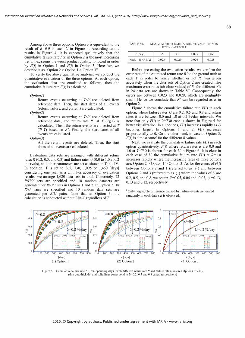
68



Among above three options, Option 3 is equivalent to the result of R=0.0 in each U in Figure 4. According to the results in Figure 4, it is expected qualitatively that the cumulative failure rate F(i) in Option 2 is the most increasing trend, i.e., seems the worst product quality, followed in order by F(i) in Option 1 and F(i) in Option 3. Hereafter, we describe it as “Option 2 > Option 1 > Option 3”.

To verify the above qualitative analysis, we conduct the quantitative evaluation of the three options. At each option,the evaluation data are emulated as follows, then the cumulative failure rate F(i) is calculated.

Option1) Return events occurring at T<Y are deleted from reference data. Then, the start dates of all events(return, failure, and current) are calculated.

Option2) Return events occurring at T<Y are deleted from reference data, and return rate R’ at T (T Y) iscalculated. Then, the return events are inserted at T(T<Y) based on R’. Finally, the start dates of all events are calculated.

Option3)All the return events are deleted. Then, the start dates of all events are calculated.

Evaluation data sets are arranged with different return rates R (0.2, 0.5, and 0.8) and failure rates U (0.0 to 1.0 at 0.2 intervals), and other parameters are set as shown in Table IV. In addition, Y is set to 365, 730, 1,095 or 1,460 [days]considering one year as a unit. For accuracy of evaluation results, we arrange 1,620 data sets in total. Concretely, 72 R/U/Y sets are specified and 10 random datasets are generated per R/U/Y sets in Options 1 and 2. In Option 3, 18 R/U pairs are specified and 10 random data sets are generated per R/U pairs. Note that at Option 3, thecalculation is conducted without List-C regardless of T.

TABLE VI. MAXIMUM ERROR RATE (ABSOLUTE VALUE) OF R’ INOPTION 2 AT EACH Y

Y [days] 365 730 1,095 1,460

Max. | R’ R | / R 0.023 0.029 0.026 0.028

Before presenting the evaluation results, we confirm the error rate of the estimated return rate R’ to the ground truth at each Y in order to verify whether or not R’ was given accurately when the data sets of Option 2 are created. The maximum error rates (absolute values) of R’ for different Y’sin 24 data sets are shown in Table VI. Consequently, the errors are between 0.023 and 0.029, which are negligiblysmall. Hence we conclude that R’ can be regarded as R in Option 2.

Figure 5 shows the cumulative failure rate F(i) in each option, where failure rates U are 0.2, 0.5 and 0.8 and return rates R are between 0.0 and 1.0 at 0.2 %/day intervals. We note that only F(i) in Y=730 case is shown in Figure 5 for better visualization. In all options, F(i) increases rapidly as Ubecomes larger. In Options 1 and 2, F(i) increases proportionally to R. On the other hand, in case of Option 3, F(i) is almost samei for the different R values.

Next, we evaluate the cumulative failure rate F(i) in each option quantitatively. F(i) where return rates R are 0.0 and 1.0 at Y=730 is shown for each U in Figure 6. It is clear in each case of U, the cumulative failure rate F(i) at R=1.0 increases rapidly where the increasing rates of three options are: Option 2 > Option 1 > Option 3. As for the errors of F(i)between Options 2 and 1 (referred to as ) and between Options 2 and 3 (referred to as ) where the values of U are0.2, 0.5, and 0.8, we obtain =0.05, 0.04 and 0.03, =0.13, 0.13 and 0.12, respectively.

i Only negligible difference caused by failure events generated randomly in each data set is observed.

Figure 5. Cumulative failure rate F(i) vs. operating days i with different return rate R and failure rate U in each Option (Y=730).(thin dot, thick dot and solid lines correspond to U=0.2, 0.5 and 0.8 cases, respectively)

0

0.2

0.4

0.6

0.8

1

0 100 200 300 400 500 600 700 800

F(i)

i [days]

0

0.2

0.4

0.6

0.8

1

0 100 200 300 400 500 600 700 800

F(i)

i [days]

0

0.2

0.4

0.6

0.8

1

0 100 200 300 400 500 600 700 800

F(i)

i [days]

U=0.2 %/day

U=0.5

U=0.8

U=0.2 %/day

U=0.8

U=0.2 %/day

U=0.5

U=0.8

(1) Option 1 (2) Option 2 (3) Option 3

U=0.2 U=0.5 U=0.8R=1.0R=0.8R=0.6R=0.4R=0.2R=0.0

[%/day] U=0.2 U=0.5 U=0.8R=1.0R=0.8R=0.6R=0.4R=0.2R=0.0

[%/day] U=0.2 U=0.5 U=0.8R=1.0R=0.8R=0.6R=0.4R=0.2R=0.0

[%/day]

U=0.5

69



Figure 6. Cumulative failure rate F(i) vs. operating days i with differenet Option/R pairs in each U value (Y=730).

Figure 7. Cumulative failure rate F(i) vs. operating days i with different Y/R pairs in each Option (U=0.5).

Furthermore, we confirm the impact of starting the maintenance of List-C at Y on the cumulative failure rate F(i). Figure 7 shows F(i) at each Y when U is 0.5. For comparing the results, in all figures, we plot Y=0 (black solid and dottedlines) as the references in which List-C is maintained from the beginning as well as List-A and List-B. In Option 2 at R=1.0, F(i) is almost the same irrespective of Y. On the other hand in Option 1, F(i) becomes larger as Y decreases. In addition, F(i) at Y>0 is smaller than that at Y=0. Furthermore, as for comparison of Options 1 and 2, F(i) in Option1 is smaller than that in Option 2 at Y=365 (the smallest value of Y in this evaluation).

These results prove the correctness of our qualitative expectation for the cumulative failure rate F(i), i.e., Option 2 > Option 1 > Option 3 (see Section VI). Note that the above order is not changed irrespective of Y, the date for starting the maintenance of List-C.

VII. CONCLUSION

In this paper we proposed a method of calculating the cumulative failure rate in IoT service infrastructure operated by multiple players such as service providers and device

vendors in the horizontal specialization business model.According to changing business environment around providers such as massive numbers of IoT devices and strenuous demand on its service availability, we believe each provider itself is also required to expand the quality management of devices instead of or together with vendors.

We revealed the possibility on lack of information from the provider’s perspective, and proposed the method which aggregates and analyzes distributed information to derive the operating history of each IoT device to enable calculation of cumulative failure rates. We also verified that the proposed method can derive operating histories and calculate the cumulative failure rate. In addition, we evaluated the accuracy of the derived cumulative failure rates when some information about device operation are missing. From the experimental evaluation, our method conservatively underestimates the cumulative failure rate. So, the calculated failure rate should be interpreted carefully according to the player’s role. Even if such underestimation exists, from the provider’s perspective, it is considered to be useful because it becomes some evidence to encourage the vendor to improve the product quality and reliability of IoT devices more.

0

0.2

0.4

0.6

0.8

1

0 100 200 300 400 500 600 700 800

F(i)

i [days]

0

0.2

0.4

0.6

0.8

1

0 100 200 300 400 500 600 700 800F(

i)i [days]

0

0.2

0.4

0.6

0.8

1

0 100 200 300 400 500 600 700 800

F(i)

i [days]

=0.05

=0.13

=0.04

=0.13

=0.03

=0.12

(1) U=0.2 %/day (2) U=0.5 %/day (3) U=0.8 %/day

Option1 R=0.0Option1 R=1.0Option2 R=0.0Option2 R=1.0Option3 R=0.0Option3 R=1.0

[%/day]Option1 R=0.0Option1 R=1.0Option2 R=0.0Option2 R=1.0Option3 R=0.0Option3 R=1.0

[%/day]Option1 R=0.0Option1 R=1.0Option2 R=0.0Option2 R=1.0Option3 R=0.0Option3 R=1.0

[%/day]

0

0.2

0.4

0.6

0.8

1

0 100 200 300 400 500 600 700 800

F(i)

i [days]

0

0.2

0.4

0.6

0.8

1

0 100 200 300 400 500 600 700 800

F(i)

i [days]

0

0.2

0.4

0.6

0.8

1

0 100 200 300 400 500 600 700 800

F(i)

i [days]

(1) Option 1 (2) Option 2 (3) Option 3

F(i)Y=0 R=0.0 (reference)

Y=0 R=1.0 (reference)Y=365 R=0.0Y=356 R=1.0Y=730 R=0.0Y=730 R=1.0Y=1095 R=0.0Y=1095 R=1.0Y=1480 R=0.0Y=1480 R=1.0

[%/day]F(

i)Y=0 R=0.0 (reference)Y=0 R=1.0 (reference)Y=365 R=0.0Y=356 R=1.0Y=730 R=0.0Y=730 R=1.0Y=1095 R=0.0Y=1095 R=1.0Y=1480 R=0.0Y=1480 R=1.0

[%/day]

Y=0 R=0.0 (reference)Y=0 R=1.0 (reference)Y=365 R=0.0Y=356 R=1.0Y=730 R=0.0Y=730 R=1.0Y=1095 R=0.0Y=1095 R=1.0Y=1480 R=0.0Y=1480 R=1.0

[%/day]

70



Furthermore, to prove wide applicability of our proposed method, we also evaluated the additional but promising uncoordinated case in which additional information elements are added after the service was launched, due to emerging new operational requirements. We quantitatively analyzed the cumulative failure rate using three types of options forcalculating methods.

We are now planning to apply our method to furtherdifferent cases. We believe that we have shown the applicability of our method by introducing well-seen,representative cases in this paper, but examination of our approach in a variety of scenarios is part of our future work.

REFERENCES

[1] M. Shibuya, Y. Hasegawa, and H. Yamaguchi, “A Study on Device Management for IoT Services with Uncoordinated Device Operating History,” Proc. International Conference on Networks (ICN 2016), pp.72-77, Feb. 2016.

[2] Cisco Systems Inc., “Cisco Visual Networking Index: Global Mobile Data Traffic Forecast Update, 2013-2018,” http://www.cisco.com/c/en/us/solutions/collateral/service-provider/visual-networking-index-vni/white_paper_c11-520862.html, accessed Jan. 8, 2016.

[3] M. Ahamad, “Reliability Models for the Internet of Things: A Paradigm Shift,” Proc IEEE International Symposium on Software Reliability Engineering Workshops, pp.52-59, Nov. 2014.

[4] M. Ahamad, “Designing for the Internet of Things: A paradigm Shift in reliability,” Proc. Electribuc Cioibebts & Technology Conference, pp.1758-1766, May 2015.

[5] M. N. Sahana, S. Anjana, S. Ankith, K. Matarajam, K. R. Shobha, and A. Paventhan, “Home energy management open IoT protocol stack,” Proc. IEEE Recent Advances in Intelligent Computational Systems (RAICS), pp.370-375, Dec.2015.

[6] S. Stanley, “MTBF, MTTR, MTTF & FIT Explanation of Terms,” http://imcnetworks.com/wp-content/uploads/2014/12/MTBF-MTTR-MTTF-FIT.pdf,accessed Sep. 16, 2016.

[7] W. Zheng, W. Zengquan, and W. A-na, “Failure Rate Calculating Method of Components Based on the Load-strength Interference Model,” Proc. IEEE Industrial Engineering and Engineering Management (IEEM 2010),pp.783-787, Dec. 2010.

[8] OPS rules, “Vertical vs. Horizontal Integration: Which is a better Operations Strategy?,” Sep. 2012, http://www.opsrules.com/supply-chain-optimization-blog/bid/241648/Vertical-vs-Horizontal-Integration-Which-is-a-Better-Operations-Strategy, accessed Jan. 8, 2016.

[9] Z. Yu, “IT, Production Specialization, and Divison of Labor: A Smith-Ricardo Model of International Trade,” Carleton Economic Paper, Jun. 2003, http://carleton.ca/economics/wp-content/uploads/cep03-06.pdf, accessed Jun. 8, 2016.

[10] R. Suoranta, “New Directions in Mobile Device Architectures,” Proc. Euromicro Conference on Digital System Design (DSD’06) , pp.17-26, Aug. 2006.

[11] Fujitsu Limited, “Management Direction Briefing,” Oct. 2015, http://pr.fujitsu.com/jp/ir/library/presentation/pdf/en/md-20151029note.pdf, accessed Aug. 8, 2016.

[12] Z. Zhou, X. Liu, Q. Shi, Y. En, and X. Wang, “Failure Rate Calculation for NMOS Devices under Multiple Failure Mechanisms,” Proc. International Symposium on the Physical and Failure Analysis of Integrated Circuits (IPFA), pp.362-365, Jul. 2013.

[13] T. Tekcan, G. Kahramanoglu, and M. Giinduzalp, “Determining Reliability by Failure Rate Estimation via a New Parameter,” Proc. Reliability and Maintainability Symposium (RAMS), pp.1-7, Jan. 2012.

[14] J. Pan. Z. Wang, amd D. Lubkeman, “Condition Based Failure Rate Modeling for Electric Network Components,” Proc. Power Systems Conference andExposition (PSCE ’09),pp.1-6, Mar. 2009.

[15] R. Wang, A. Xue, S. Huang, X. Cao, Z. Shao, and Y. Luo, “On the Estimation of Time-Varying Failure Rate to Protection Devices Basedon Failure Pattern,” Proc. Electric Utility Deregulation and Restructuring and Power Technologies (DRPT), pp.902-905, Aug. 2011.

[16] Q. Duan and J. Liu, “Modelling a Bathtub-Shaped Failure Rate by a Coxian Distribution,” Proc. IEEE Transactions on Reliability, vol. 65, issue 2, pp.878-885, Jun. 2016.

[17] P. James and A. Forsyth, “Real time, on line, age calculation of IGBT power modules,” Proc. Power Electronics, Machines and Drives (PEMD 2010), pp.1-4, Apr. 2010.

[18] A. J. Henry and J. A. Nachlas, “An equivalent age model for condition-based maintenance,” Proc. Reliability and Maintainability Symposium (RAMS), pp.1-6, Jan. 2012.

[19] H. Funakoshi and T. Matsukawa, “A failure Rate Estimation Considering the Change in the Number of Equipments,” IEICE Trans. B Vol. J93-B No.4, pp.681-692, 2010 (in JAPANESE).

[20] H. Funakoshi and T. Matsukawa, “A Failure Rate Estimation Considering the Change in the Number of Equipments -Applicable condition of mathematical model for proposed method -,” IEICE NS2009-17, pp.1-6, 2009 (in JAPANESE).

[21] M. Xie, Y. Tang, and T. N. Goh, “A modified Weibull extension with bathtub-shaped failure rate function,” Reliability Engineering and System Safety, 2002, 76(3): 279-285.

[22] Z. Sheng, H. Wang, C. Yin, X. Hu, S. Yang, and V. C. M.Leung, “Lightweight Management of Resource-Constrained Sensor Devices in Internet of Things,” in IEEE Internet of Things Journal, vol.2, no.5, pp.402-411, Oct. 2015.

[23] C. Zhou and X. Zhang, “Toward the Internet of Things application and management: A practical approach,” in IEEE WoWMoM 2014, pp.1-6, 2014.

[24] S. N. Han, S. Park, G.M. Lee, and N. Crespi, “Extending the Devices Profile for Web Services Standard Using a REST Proxy,” in IEEE Internet Computing, vol.19, no.1, pp.10-17, Jan.-Feb. 2015.

[25] Z. Sheng, C. Mahapatra, C. Zhu, and V. C. M. Leung, “Recent Advances in Industrial Wireless Sensor Networks Toward Efficient Management in IoT,” in IEEE Access, vol.3,pp.622-637, May 2015.

[26] G. Chen, J. Huang, B. Cheng, and J. Chen, “A Social Network based Approach for IoT Device Management and Service Composition,” Proc. IEEE World Congress on Services 2015, pp.1-8, Jun. 2015.

[27] B. Manate, T. Fortis, and V. Negru, “Infrastructure Management Support in a Multi-Agent Architecture for Internet of Things, ” Proc. Modelling Symposium (EMS), pp.372-377, Oct. 2014.

[28] Freepress, “That Box Your Cable Company Forces You to Rent,” May 2016, http://www.freepress.net/blog/2016/05/20/box-your-cable-company-forces-you-rent, accessed Nov. 22, 2016.

71



SDN Solutions for Switching Dedicated Long-Haul Connections:Measurements and Comparative Analysis

Nageswara S. V. Rao

Oak Ridge National LaboratoryOak Ridge, TN 37831, USAEmail: [email protected]

Abstract—We consider a scenario of two sites connected overa dedicated, long-haul connection that must quickly fail-over inresponse to degradations in host-to-host application performance.The traditional layer-2/3 hot stand-by fail-over solutions donot adequately address the variety of application degradations,and more recent single controller Software Defined Networks(SDN) solutions are not effective for long-haul connections. Wepresent two methods for such a path fail-over using OpenFlow-enabled switches: (a) a light-weight method that utilizes hostscripts to monitor application performance and dpctl API forswitching, and (b) a generic method that uses two OpenDaylight(ODL) controllers and REST interfaces. For both methods, therestoration dynamics of applications contain significant statisticalvariations due to the complexities of controllers, north boundinterfaces and switches; they, together with the wide varietyof vendor implementations, complicate the choice among suchsolutions. We develop the impulse-response method based onregression functions of performance parameters to provide arigorous and objective comparison of different solutions. Wedescribe testing results of the two proposed methods, usingTCP throughput and connection rtt as main parameters, over atestbed consisting of HP and Cisco switches connected over long-haul connections emulated in hardware by ANUE devices. Thecombination of analytical and experimental results demonstratethat the dpctl method responds seconds faster than the ODLmethod on average, even though both methods eventually restoreoriginal TCP throughput.

Keywords–Software defined networks; OpenFlow; Opendaylight;controller; long-haul connection; impulse-response; testbed.

I. INTRODUCTION

We consider scenarios where two remote sites are con-nected over a dedicated long-haul connection with hundredsof millisecond latency, such as a transcontinental fiber orsatellite link [1], as illustrated in Figure 1(a). Different client-server application pairs are executed at different times on hostsystems located at the sites, which range from data transfersto on-line instrument monitoring to messaging. Applicationsmay incorporate different methods to account for networklosses and jitter; for example, they may utilize TCP or UDTfor guaranteed delivery, UDP for loss tolerant cases, custombuffering methods and others at application level to accountfor jitter. Furthermore, their performance may be optimizedor customized to connection parameters such as latency, jitterand loss rate; for example, TCP parameters may be tuned forlong-haul connections and buffers of interactive codes maybe tuned for long latencies and jitter of satellite links. Theconnection quality can degrade due to a variety factors suchas equipment failures, weather conditions, and geographicalevents, which may be reflected in host-to-host applicationperformance. Indeed, the client-server application pairs mayrespond differently to various degradations, such as decreasedthroughput of file transfers, increased jitter in streaming, loss

host

host

host

host

host

host

host

host

fiber

fiber

border switch

border switch

transcontinental connections

satellite connections

end site

end site

end site

end site

border switch

border switch

(a) host-to-host application pairs

host

host

end site end site

application client

application performance

monitor

application performance

monitor

application server

border switch

border switch

end-to-end application performance monitoring

path switching triggers

(b) two connection modalities

Figure 1. Two sites connected over long-haul connections.

of end-to-end control in computational steering, and in somecases (such as messaging) having very little effect. As a miti-gation strategy, a physically diverse and functionally equivalentstandby path is switched to when the performance of currentlyrunning application pairs degrades.

The performances of application pairs are continuouslymonitored on host systems, and the current primary path isswitched out when needed, for example, by modifying VirtualLocal Area Networks (VLAN) and route tables on borderswitches and routers, respectively. In our use cases, humanoperators watch host-level performance monitors, and invokeCommand Line Interface (CLI) commands or web-based in-

72



terfaces of network devices for path switching. Typically, thepath fail-overs are accomplished either by manual configu-ration or through device-specific scripts. Since triggers forpath switching are dynamically generated by application pairs,they are not adequately handled by conventional hot standbylayer-2/3 solutions that solely utilize connection parameters.For example, certain losses may be tolerated by messagingapplications but not by monitoring and control applications ofinstruments and sensors. Currently, the design and operationof such application-driven fail-over schemes require a detailedknowledge of host codes, and the specialized interfaces andAPIs of switches, such as custom TL1, CURL and pythonscripts, which currently vary significantly among vendor prod-ucts. Furthermore, in our use cases such fail-over operationsmust be coordinated between two physically-separated opera-tions centers located at the end sites. The combination of recentadvances in host and network virtualization technologies [2]offers very promising and potentially game changing solutionsto seamlessly automate the dynamic fail-over workflows thatintegrate diverse application monitors and network elements.

We are interested in exploiting the network and hostvirtualization layers to unify and automate such monitoringand path switching operations. Automated scripts for thesetasks provide the following advantages over current practices:(i) improved response time, since scripts can be executedmuch faster than manual configurations, (ii) reductions inperformance degradations due to human errors in applicationmonitoring and path switching, and (iii) reductions in siteoperations costs of host systems and network devices.

A. SDN SolutionsThe rapidly evolving Software Defined Networks (SDN)

technologies [3], [4] seem particularly well-suited for automat-ing the path switching tasks, when combined with host moni-toring codes. In particular, the northbound interfaces of SDNcontrollers can be used to communicate the path degradationsinformation to trigger path switching; then, the path can beswitched by installing flow entries that divert traffic onto thestandby path using the southbound controller interfaces [5].Thus, SDN technologies provide two distinct advantages overcurrent network operations:

(a) trigger modules of new applications can be “droppedin place” with no no major software changes by usingcommunications via generic northbound interfaces, and

(b) switches from different vendors with virtual interfaces canbe simply be swapped, avoiding the re-work often neededto account for custom interfaces and operating systems.

While the problem space of our use cases is somewhat straight-forward, their SDN solution space is much more complex: dueto the rapid developments in underlying technologies, these isa wide array of choices for controllers and switches, which inturn leads to a large number of solution combinations. Indeed,their complexity and variety requires systematic analysis andcomparison methods to assess their operational effectivenessand performance, such as recovery times. In addition, com-pared to certain data-center and network provisioning scenariosfor which SDN technologies have been successfully applied,these long-haul scenarios present additional challenges. First,single controller solutions are not practical for managing theborder switches at end sites due to the large latency. Second,

solutions that require a separate control-plane infrastructurebetween the controllers and switches are cost prohibitive, insharp contrast to the connection-rich data-center or Internetscenarios.

B. Outline of ContributionsIn this paper, we present automated software solutions for

path fail-over by utilizing two controllers, one at each site,that are coordinated over a single connection through mea-surements. We first describe a light-weight, custom designeddpctl method1 for OpenFlow border switches that uses hostLinux bash scripts to: (i) monitor the connection parameters,such as rtt or TCP throughput, at the host-level and detectdegradations that require a fail-over, and (ii) utilize dpctl APIto install and delete flow entries on the border switches toimplement path fail-over when needed. This script is abouthundred lines of code, which makes it easier to analyze forits performance and security aspects. We then present a moregeneric ODL method that utilizes two OpenDaylight Hydro-gen (ODL) controllers [6] located at the end sites. We useREST interface of ODL controller to communicate the triggerinformation for path switching in the form of new OpenFlowentries to be installed on border switches. We also utilize Linuxbash scripts to monitor the connection performance to gener-ate fail-over triggers, and invoke python REST API scriptsto communicate new flow entries to ODL controllers. Theexecutional path of this approach is more complex comparedto the dpctl method since it involves communications usingboth northbound and southbound ODL interfaces and invokingseveral computing modules within ODL software stack. Thus,a complete performance and security analysis of this methodrequires a closer examination of much larger code base thatincludes both host scripts and corresponding ODL modules,including its embedded http server.

We present implementation and experimental results usinga testbed consisting of Linux hosts, HP and Cisco borderswitches, and ANUE long-haul hardware connection emulationdevices. We utilize TCP throughput as a primary performancemeasure 2 for the client-server applications, which is effectedby the connection rtt and jitter possibly caused by pathswitching, and the available path capacity. Experimental resultsshow that both dpctl and ODL methods restore the host-to-hostTCP throughput within seconds by switching to the standbyconnection after the current connection’s RTT is degraded (byexternal factors). However, the restoration dynamics of TCPthroughput show significant statistical variations, primarily asa result of interactions between the path switching dynamics ofcontrollers and switches, and the highly non-linear dynamicsof TCP congestion control mechanisms [7]–[9]. As a result,direct comparisons of individual TCP throughput time tracescorresponding to fail-over events are not very instructive inreflecting the overall performance of the two methods.

To objectively compare the performance of these tworather dissimilar methods, we propose the impulse-response

1Note that dpctl is originally intended for diagnosis purposes, which weutilize as a controller.

2The overall approach is applicable to other application-level performancemeasures such as response times, which typically degrade under connectiondisruptions and recover when connection is restored. Our choice of TCPis based on its widespread use for guaranteed packet delivery and its richdynamics.

73



method that captures the average performance by utilizingmeasurements collected in response to a train of path degra-dation events induced externally. We establish a statisticalbasis for this method using the finite-sample theory [10] byexploiting the underlying monotonic properties of performanceparameters during the degradation and recovery periods. Thisanalysis enables us to objectively conclude that on the averagethe dpctl method restores the TCP throughput several secondsfaster than the ODL method for these scenarios. This paper isan expanded version of an earlier conference paper [1] withadditional explanations and details of SDN implementations,and it also provide a complete derivation of the performanceequations for the impulse response method using finite samplestatistical analysis.

The organization of this paper is as follows. Two-site sce-narios with dedicated long-haul connections are described inSection II. A coordinated controllers approach for connectionfail-over, and its implementation using dpctl and ODL methodsare described in Section III. An experimental testbed consistingof Linux servers and HP and Cisco switches is described inSection IV-A, and the results of experiments using dpctl andODL methods using five different configurations are presentedin Section IV-B. The impulse response method to assess theoverall fail-over performance is presented in Section V-A, andits statistical basis is presented in Section V-B. Conclusionsare presented in Section VI.

II. LONG-HAUL CONNECTION SWITCHING

We consider scenarios consisting of two sites connectedover a long-haul connection such as transcontinental fiberroutes or satellite connections as shown in Figure 1(a). Thesites house multiple workstations on which server and clientapplications are executed, which form the client-server appli-cation pairs over the long-haul connection as shown in Figure1(b). The client-server application performance depends onthe quality of the connection specified by parameters such aslatency, loss rate, and jitter. These connection parameters maydegrade due to external factors such as equipment failures,fiber cuts and weather events. Such factors will be reflectedin the degradation in client-server performance, which may bedetected by the performance monitoring software implementedat application-level, for example, using Linux scripts. To pro-tect against such factors, a parallel standby path is provisionedthat can be switched-over to when performance degradationsare detected. The border switches or routers at the sites areconnected to both the primary long-haul connection that carriesthe traffic, and the stand-by connection whose traffic canbe activated as needed. In our case, these connections areimplemented as layer-2 VLANS at the border switches, whichcan be modified to implement the fail-over. All traffic betweenthe sites is carried by the single long-haul connection, in-cluding client-server communications and other traffic neededfor coordinating network operations; in particular, it is notcost-effective to provision a separate “control” connection forsupporting the network configuration operations unlike in othercases, such as in UltraScienceNet [11] a decade ago and morerecently in SDN based solutions.

Application codes on host systems continually monitor theclient-server performance, such as iperf for TCP throughputand UDP loss rate. Under path degradations, these parameterswould be out of normal range, and such events are detected

dpctl controller

linux host

OpenFlow switch dpctl

app

perf api

OpenFlow

10GigE

Performance app + REST interface + odl controller

linux host

linux host

OpenFlow switch

perf app

ODL http

server

REST interface

OpenFlow

10GigE

http

(a)

(b)

Figure 2. Configurations of dpctl and ODL controllers.

and alerts are sent to network operations. Typically, humanoperators receiving the alerts modify the VLANS on borderswitches to implement path switching, for example, by invok-ing CLI or TL1 or curl scripts, or manually making the changesthrough CLI or web interfaces. Due to different organizationalzones at the sites and the long separation between them, it isnot practical for a single network operations center to handleconnection switching at both sites, particularly, if the same“degraded” connection is used for these communications aswell. Instead, such tasks are typically coordinated between thetwo site organizations using other means such as telephonecalls. Due to the multi-step process needed here, the fail-over operation can take anywhere between few minutes tohours. Thus, it is highly desirable to automate the entire fail-over work flow that includes application-level monitoring andnetwork-level switching as described in Introduction section.

III. COORDINATED SDN CONTROLLERS

For the long-haul scenarios considered here, a singlecontroller solution is not effective, although such approacheswith stable control-plane connections have been effective inpath/flow switching over local area networks using OpenFlow[12], [13] and cross-country networks using customized meth-ods [11], [14]. Since the controller has to be located at asite, when primary connection degrades, it may not be able tocommunicate effectively with the remote site. Our approachis to utilize two controllers, one at each site, which are “in-directly” coordinated based on the monitored application-levelperformance parameters. When path degradation is inferred bya host script, the controller at that site switches to the fail-overpath by installing the appropriate flow entries on its borderswitch. If the primary path degrades, for example, resulting inincreased latency or loss rate, its effect is typically detected atboth hosts by the monitors, and both border switches fail-overto the standby path approximately at the same time. If borderswitch at one site fails-over first, the connection loss will bedetected at the other site which in turn triggers the fail-over atthe second site. Also, one-way failures lead to path switchingat one site first, which will be seen as a connection loss at theother site, thereby leading to path switching at that site as well.Due to recent developments in SDN technologies, both in open

74



software [3], [4], [15] and specific vendor implementations[16], [17], there are many different ways such a solution canbe implemented. We restrict here to OpenFlow solutions basedon open standards and software [12].

A. dpctl Method

As a part of OpenFlow implementation, some vendorssupport dpctl API which enables hosts to communicate withswitches to query the status of flows, insert new flows anddelete existing flows. It has been a very useful tool primarilyfor diagnosing flow implementations by using simple hostscripts; however, some vendors such as Cisco do not providedpctl support. We utilize dpctl API in a light-weight host scriptthat constantly monitors the connection rtt and detects when itcrosses a threshold and invokes dpctl to implement the fail-overas shown in Figure 2(a). The OpenFlow entries for switchingto the standby path are communicated to the switch uponthe detection of connection degradation. This script consistsof under one hundred lines of code and is flexible in thatthe current connection monitoring module can be replacedby another one such as TCP throughput monitor using iperf.Compared to methods that use separate OpenFlow controllers,this method compresses both performance monitoring andcontroller modules into one script, and thereby avoids thenorthbound interface altogether; for ease of reference, we referto this host code as the dpctl controller. This small footprint ofthe code makes is easier to analyze both from performance andsecurity perspectives. Also, the executional path of this codeis very simple since it involves application monitoring directlyfollowed by communications with the switch; in particular, thismethod does not require a separate controller that is constantlyrunning at the end sites.

B. OpenDaylight Method

We now present a method that utilizes two ODL Hy-drogen controllers and REST interfaces to implement fail-over functionality using OpenFlow flows as shown in Figure2(b). ODL is an open source controller [6] that communicateswith OpenFlow switches 3, and is used to query, install anddelete flow entries on them using its southbound interface.The applications communicate with ODL controller via thenorthbound interface to query, install and delete flows. ODLsoftware in our case runs on linux workstations called thecontroller workstations, and the application monitoring codescan be executed on the same workstation in the local modeor can be executed on a different workstation in the remotemode.

The same performance monitoring codes of the dpctlmethod above are used in this case to detect path degradationsbut are enhanced to invoke python code to communicatenew flows for switching paths to ODL controllers via RESTinterfaces; the content of these flow entries are identical toprevious case. Thus, both the software and executional pathsof this method are much more complicated compared toprevious case, and also the ODL controllers are required torun constantly on the servers at end sites. Also, this Hydrogen

3ODL provides interfaces to much broader classes of switches and appli-cations, but we limit our discussions to the functionalities that are directlyrelated to long-haul scenarios described in Section II.

linux workstation

long-haul connection emulation

server/client host

linux workstation

ANUE OC192 emulator

ANUE 10GigE emulator

controller host

OpenFlow switch

Cisco 3064

HP 5406zl

two OpenFlow switches

OpenFlow switch

linux workstation

controller host

server/client host

linux workstation

Figure 3. Testbed of two sites connected over local fiber and emulatedconnections.

ODL code4 is much more complex to analyze since it involvesnot only the REST scripts but also the ODL stack which byitself is a fairly complex software. The execution path is morecomplex since it involves additional communication over bothnorthbound and southbound interfaces of ODL controllers.

The dpctl and ODL methods represent two different fail-over solutions, and the choice between them depends on theirrecovery performance in response to triggers. In the nextsection, we describe a set of experiments using HP and Ciscoswitches that highlight the performances of controllers andswitches. However, a direct comparison of the measurementsbetween various configurations is complicated by their sta-tistical variations, which we account for using the impulseresponse method described in Section V.

IV. EXPERIMENTAL RESULTS

In this section, we first describe the details of testbed andtests using dpctl and ODL controllers, and then describe theexperimental results.

A. Emulation TestbedThe experimental testbed consists of two site LANs each

consisting of multiple hosts connected via 10GigE NICs tothe site’s border switch. The border switches are connectedto each other via local fiber connection of few meters inlength and ANUE devices that emulate long-haul connectionsin hardware, as shown in Figure 3. Tests are performed inconfigurations that use pairs of HP 5064zl and Cisco 3064devices as border switches. These switches are OpenFlow-enabled but only HP switches support dpctl interface. We onlyutilize OC192 ANUE device in our tests, which can emulatertts in the range of [0-800] milliseconds with a peak capacityof 9.6 Gbps. These devices are utilized primarily to emulatethe latencies of long-haul connections, both transcontinental

4Later ODL releases starting with Helium, including Lithium and Beryllium,support more agile code builds wherein only the needed service modules areloaded (as karaf features [6]), thereby significantly reducing its size. Howeverthe execution path remains the same as in Hydrogen.

75



fiber and satellite connections, to highlight the overall recoverydynamics. However, no efforts are made to highlight their ca-pacity differences, for example, by limiting the latter to typicalsatellite connection capacities, which could have resulted insomewhat muted dynamics. The conversion between 10GigELAN packets from the border switches and long-haul OC192ANUE packets is implemented using a Force10 E300 switch,which provides 10GigE LAN-PHY and WAN-PHY conversionas shown in Figure 4.

feynman 1

feynman 2

feynman 3 3

feynman 4

HP 5406zl

HP 5406zl

e300 10GE-OC192

ANUE OC192

odl app

odl app

odl

odl

loop back

feynman 3

feynman 4 iperf

TCP iperf TCP

Simulated degraded path: long-haul emulation: latency 30 ms

(a) Configurations C-E: remote

feynman 1

feynman 2

HP 5406zl

HP 5406zl

e300 10GE-OC192

ANUE OC192

odl app

odl app

odl

odl

loop back

Simulated degraded path: long-haul emulation: latency 30 ms

feynman 1

feynman 2 iperf

TCP iperf TCP

(b) Configuration B: local

Figure 4. Remote and local modes of ODL controller configurations.

Two classes of Linux hosts are connected to the borderswitches. The controller hosts (feynman1 and feynman2) areutilized to run ODL controllers, and client and server hosts(feynman3 and feynman4) are used to execute monitoring andtrigger codes along with client server codes, for example iperfclients and servers. Five different configurations are employedin the tests as shown in Table I. The dpctl tests utilize onlythe client and server hosts to execute both monitoring andswitching codes. In these tests, dpctl is used to communicateflow modification messages between the hosts and HP 5064zlswitches, and Cisco switches are not used. ConfigurationA corresponds to these tests with the monitoring and dpctl

Table I. Five test configurations with two controllers, two connectiondegradation methods and two switch vendors.

test controller path switchconfiguration method degradation vendor

A dpctl path switch HPB ODL local path swith HPC ODL remote path switch HPD ODL remote rtt extension HPE ODL remote rtt extension Cisco

scripts running on server/client hosts, and it uses HP borderswitches. For ODL remote mode tests, the monitoring codes onclient/server hosts utilize REST interface to communicate flowmessage needed for fail-over; both HP and Cisco switches areused in these tests. Configurations C-E implement these tests,which employ ODL controllers running on controller hostsand monitoring scripts running on server/client hosts. In ODLlocal mode tests, the monitoring and client/server codes areexecuted directly on control hosts. Configuration B implementsthese tests, and it is identical to Configuration C except itsscripts are executed on controller hosts. The measurements inConfigurations B and C are quite similar, and hence we mostlypresent results of the latter.

In the experiments, connection degradation events are im-plemented by external codes using two different methods:

(a) Path switching using dpctl: The current physical path witha smaller rtt is switched to a longer emulated path, whosertt is sufficient to trigger the fail-over. This switchingis accomplished by using dpctl or ODL by installingOpenFlow entries on the border switches to divert theflow from the current path to longer path. The packetsenroute on the current path will be simply be droppedand as a result the short-term TCP throughput becomeszero. After the fail-over, the path is switched back to theoriginal path, and the TCP flow recovers gradually backto previous levels.

(b) RTT extension using curl scripts: The current connec-tion’s rtt is increased by changing the setting on ANUEdevice to a value above the threshold to trigger the fail-over. This is accomplished using http interface eithermanually or using curl scripts. Unlike the previous case,the packets enroute on the current path are not droppedbut are delayed; thus, the instantaneous TCP throughputdoes not always become zero but is reduced significantly.After the fail-over, the original rtt is restored, and TCPthroughput recovers gradually to previous levels.

The first degradation method using dpctl to switch the paths isonly implemented for configurations with HP border switchesin Configurations A - C. The second method is used for bothHP and Cisco system in Configurations D and E, and since thecurl scripts are used here to change delay settings on ANUEdevices, and border switches are not accessed.

B. Controller PerformanceTCP throughput measurements across the long-haul con-

nection are constantly monitored using iperf. The defaultCUBIC congestion control module [18] for Linux hosts isused in all tests. The rtt between end hosts is also constantlymonitored using ping, and path switching is triggered whenit crosses a set threshold; this module can be replaced by a

76



more general application-based trigger module, for example, todetect when throughput falls below or jitter exceeds thresholds.The path degradations are implemented as periodic impulsesand the responses are assessed using the recovery profiles ofTCP throughput captured at one second intervals. Also, theANUE dynamics in extending the rtt affect the TCP throughputrecovery, and we obtain additional baseline measurements byutilizing a direct fiber connection that avoids packets beingrouted through ANUE devices. Thus, TCP throughout tracesin our tests capture the performances of: (a) controllers,namely, dpctl and ODL, in responding to fail-over triggersfrom monitoring codes, and in modifying the flow entries onswitches, typically by deleting the current flows and insertingthe ones for standby path, and (b) border switches in modifyingthe flows entries in response to controller’s messages and re-routing the packets as per new flow entries.

Example Trace:

path switch

TCP throughput loss

latency increase

input impulse train

throughput

rtt

Figure 5. Trace of impulse response of TCP throughput for dpctl methodwith local primary path and path switching degradation.

An example TCP throughput trace of a test run in Config-uration A is shown in Figure 5 for the dpctl method, with fiberconnection as the primary path, and using the path switchingdegradation method. The connection rtt is degraded at theperiodicity of 50 seconds by externally switching to the longerANUE path, and the change is detected as shown in the bottomplot, which in turn triggers the fail-over. TCP throughputparameters on the hosts are tuned to achieve 10Gbps for thedefault rtt, and it degrades once the connection rtt is increasedto 30ms after path switching. Upon the detection of increasedrtt, the default path is restored, which in turn restores TCPthroughput to the original value as shown in the middle plotof Figure 5. Note that throughput trace shows significantvariations during the recovery periods following the fail-over,even in this simplest among the test configurations.

The restoration profiles of TCP throughput in these testsreflect the detection of connection degradation and fail-over,followed by the recovery response of the non-linear dynamicsof CUBIC congestion control mechanism. Three different TCPrecovery profiles from the tests are shown in Figure 6: (a)

50 100 150 200 250 300 350 400 450 5001

2

3

4

5

6

7

8

9

10

11

time (sec)

Gbp

s

TCP throughput profiles

dpctl−hp−localodl−hp−anueodl−cisco−anue

Figure 6. TCP throughput for dpctl method for configuration A and ODLmethods for configuration D and E.

Configuration A: dpctl method using HP switches with con-nection degradation by path switching, (b) Configuration D:ODL method using HP switches with connection degradationby rtt extension, and (c) Configuration E: ODL method usingCisco switches with connection degradation by rtt extension.As seen in these plots, TCP response dynamics contain sig-nificant variations for different degradation events of the sameconfiguration as well as between different configurations.

The individual TCP throughput recovery responses tosingle path degradation events reveal more details of thedifference between configurations as shown in Figure 7. Thedelayed response of ODL method compared to dpctl methodcan be seen in Figure 7(a) for Configurations A and B.Since the packets in transit during the switching are simplylost during path switching, the instantaneous TCP throughputrapidly drops to zero for Configuration A. On the otherhand, some of the packets in transit when rrt is extendedare delivered, and as a result TCP throughput may be non-zero in some cases, as shown in Figure 7(b). Another aspectis that, TCP throughput recovers to 10Gbps when the directfiber connection is used between the switches, but only peaksaround 9 Gbps when packets are sent via ANUE connectionwith zero delay setting as shown in Figure 7(b). Also, therecovery profiles are different between HP and Cisco switchesin otherwise identical Configurations E and F as shown inFigure 7(c). Thus, TCP dynamics depend both on the controllerprimarily in terms of recovery times, and on the switchesin terms of the peak throughput achieved and its temporalstability.

We now consider more details of the dpctl and ODLmethods using HP switches with path switching degradationshown in Figure 7(a) with the primary fiber connection. Here,the TCP throughput becomes zero and rtt crosses the thresholdimmediately following the path switching degradation, andboth controllers respond to the fail-over triggers and switchthe path back to original fiber connection. Since these config-urations are identical except the controllers, the recovery timeof ODL method is a few seconds slower than dpctl method.However, the complex dynamics and statistical variations ofTCP profiles make it harder to draw general conclusionsabout their comparative performance based on such singledegradation events.

77



10 20 30 40 50 60 70 80 90 1001

2

3

4

5

6

7

8

9

10

11

time (sec)

Gbp

s


dpctl−hp−localodl−hp−local

(a) Configurations A and B

10 20 30 40 50 60 70 80 90 1001

2

3

4

5

6

7

8

9

10

11

time (sec)

Gbp

s


dpctl−hp−localodl−hp−anue

(b) Configurations A and D

10 20 30 40 50 60 70 80 90 1001

2

3

4

5

6

7

8

9

10

11

time (sec)

Gbp

s


odl−hp−anueodl−cisco−anue

(c) Configurations D and E

Figure 7. Trace of impulse response of TCP throughput for dpctl methodwith local primary path and path switching degradation.

C. Switch Performance

TCP performance is effected by the path traversed bythe packets between the border switches, in addition to itsdependence on dpctl and ODL methods as described in theprevious section (Figure 7(b)), thereby indicating the effectsof the connection modality on client-server performance. Inconfigurations A and B, the primary connection is few me-ters of fiber between the switches, and TCP throughput isrestored to around 10 Gbps after the fail-over as shown inFigure 7(a). In Configurations D and E, the packets are sent

through the emulated connection, which consists of long-haulForce10 E300 switch and OC192 ANUE emulator with thepeak capacity of 9.6 Gbps. In this case, both peak value andthe dynamics of TCP throughput are effected as shown inFigure 7(b); as expected, the peak is below 9.6 Gbps but thereare significant variations in the throughput. Furthermore, theconnection modality effects HP and Cisco switches differentlyas shown in Figure 7(c) in that the latter reached somewhatlower peak throughput and exhibited larger fluctuations 5.

Although we focussed on TCP throughput measurementsin this section, the overall approach is applicable to otherperformance parameters such as latency in reporting sensormeasurements, response times of remote control operations,and loss of quality in voice and video transmissions. Ingeneral, we consider that the chosen performance parameterdegrades when the current connection properties degrade, andit recovers when stand-by connection is restored. This overallcharacterization is used to develop a method to systematicallycompare the measurements under different configurations.

V. IMPULSE RESPONSE METHOD

We present the impulse response method in this sectionthat captures the overall recovery response by “aggregating”generic (scalar) performance measurements (such as TCPthroughput as in previous section) collected in response toperiodic connection degradations. It enables us to objectivelycompare the performances of different methods and devicesby extracting the overall trends from measurement traces ofmultiple fail-over events. While our discussion is centeredaround TCP measurements described in the previous section,the overall approach is more generically applicable for compar-ing configurations with different controllers and switches, andit is particularly useful when the recovery throughput tracesare not amenable to simple, direct comparisons.

A. Response Regression FunctionA configuration X that implements the fail-over is specified

by its SDN controller and switches that implement the fail-over, and also the monitoring and detection modules thattrigger it. Let δ(t − iT ), i = 0, 1, . . . , n denote the inputimpulse train that degrades the connection at times iT + TD,where t represents time, T is the period between degradationsand TD < T is the time of degradation event within the period.Let TX(t) denote the parameter of interest at time t, suchas TCP throughput, as shown in Figure 6 for configurationsX=A,D,E. Let RX(t) = B − TX(t) denote the responsethat captures the “unrealized” or “unused” portion of the peakperformance level B. For example, over a connection withcapacity B it is the residual bandwidth at time t above TCPthroughput TX(t); it is close to zero when throughput is closeto the peak and it is close to B during the fail-over period whenthroughput is close to zero. We define the impulse responsefunction RX(t) such that

RXi (t) = RX(t− iT ), t ∈ [0, T )

is the response to ith degradation event δ(t − iT ), for i =0, 1, . . . , n. An ideal impulse response function is also an

5No connection-specific TCP optimizations are performed in these tests,and it is quite possible that different optimizations may be needed to achievecomparable throughput in these two configurations.

78



0 5 10 15 20 25 30 35 40 45 500

1

2

3

4

5

6

7

8

9

10

time (sec)

Gbp

s

averged impulse

A:dpctl−hpB:odl−hpC: remote−odl−hpD:remote−odl−ciscoE: remote−odl−cisco−anue

Figure 8. Examples of impulse response functions for Configurations A-Efor a single path degradation.

impulse train that matches the input, wherein each impulse rep-resents the instantaneous degradation detection, fail-over andcomplete recovery the parameter. But in practice, each RXi (t)is a “flattened” impulse function whose shape is indicative ofthe effectiveness of the fail-over. In particular, its leading edgerepresents the effect of degradation and its trailing edge repre-sents the recovery, and the narrower this function is the quickeris the recovery. Examples of RX1 (.) are shown Figure 8 forconfigurations A-E; these TCP measurements show significanttemporal variations that persist across the different degradationevents, which make it difficult to objectively compare thesesingle-event time plots. In general, such variations are to beexpected in other performance parameters such as latency andresponse time associated with sensor and control applications.Nevertheless, certain general trends seem apparent such as thefaster TCP response of the dpctl method compared to the ODLmethod.

We define the response regression of configuration X as

RX(t) = E[RXi (t)

]=

∫RXi (t)dPRX

i (t),

for t ∈ [0, ), where the underlying distribution PRXi (t) is

quite complex in general since it depends on the dynamicsof controllers, switches, end hosts, application stack and mon-itoring and detection modules that constitute X . It exhibitsan overall decreasing profile for t ∈ [0, TD + TI ] followedby an increasing profile for t ∈ (TD + TI , T ], where TI isthe time needed for the application to react to connectiondegradation. After the fail-over, TCP measurements exhibit anoverall increasing throughput until it reaches its peak as itrecovers after becoming nearly zero following the degradation.We consider that a similar overall behavior is exhibited by thegeneral performance parameters of interest.

We define the response mean Ri(t) of Ri(t) using thediscrete measurements collected at times t = jδ, j =0, 1, ..., T/δ, as

RX(jδ) =1

n

n∑i=1

(RXi (jδ)

)which captures the average profile. Examples of RXi (.) forTCP throughput are shown Figure 9 for different configurations

0 10 20 30 40 500

2

4

6

8

10

time (sec)

Gbps

averged impulse

AC

0 10 20 30 40 500

2

4

6

8

10

time (sec)

Gbps

averged impulse

AD

0 10 20 30 40 500

2

4

6

8

10

time (sec)

Gbps

averged impulse

DE

0 10 20 30 40 500

2

4

6

8

10

time (sec)

Gbps

averged impulse

ACDE

Figure 9. Impulse response regressions for n = 10 and T = 50 sec: (a)top-left: A and C, (b) top-right: A and D, (c) bottom-left: D and E , and (d)

bottom-right: all.

0 5 10 15 20 25 30 35 40 45 500

1

2

3

4

5

6

7

8

9

time (sec)

Gb

ps

averaged impulse response

dpctlremote−odl

(a) response means

(b) delay histogram

Figure 10. Comparison of response means of dpctl (configuration A) andODL (configuration C) methods using 100 path degradations with T = 50

seconds.

79



based on 10 path degradations with T = 50 seconds betweenthem, which show the following general trends.

• The dpctl method responds seconds faster than ODLmethod as indicated by its sharper shape although theirleading edges are aligned as shown in Figure 9(a).

• The connection degradation implemented by the rtt ex-tension has a delayed effect on reducing the throughputcompared to the path switching degradation method asindicated by its delayed leading edge in Figure 9(b).

• The dynamic response of regression profiles of HP 5604zland Cisco 3064 switches are qualitatively quite similaras shown in Figure 9(c), but the latter achieved some-what lower peak throughput overall; note that the largerthroughput variations at individual switching events of thelatter case are “averaged” in these plots.

In view of the faster response of dpctl method, we collectedadditional measurements in configurations A and C using100 path degradations, and the resultant response means aresomewhat smoother compared to 10 degradations as shown inFigure 10 (a) for both dpctl and ODL methods. Furthermore,the response mean of ODL method remained consistent withmore measurements, and a histogram of the relative delays ofODL method compared to dpctl method is plotted in Figure10(b), and they are in the range of 2-3 seconds in majority ofcases. These measurements clearly show the faster responseof the dpctl method for these scenarios. Such performance isexpected because of its much simpler code and execution path,both in terms of computation and communication.

In general, dpctl is primarily intended for diagnostic pur-poses and has not been used for control, and as a result itsperformance for the latter has not been investigated much,in particular, its scalability with respect to the number offlow entries. We tested the effectiveness of dpctl method withrespect to the number of flow entries used for path switching;in above tests, for each path fail-over, two flow entries areused by both dpctl and ODL methods on each border switch.We increased the number of additional flow entries to 10and 100 for each fail-over in dpctl method, and the resultantTCP throughput measurements are shown in Figure 11(a),along with those of the original ODL method. The impactof additional flow entries in dpctl method is not apparentfrom a visual inspection of these plots, primarily due to TCPthroughput variations. The response means for these cases areplotted in Figure 11(b) which show no significant differencesdue to the additional flow entries. But, they show that theresponse of dpctl method is still 2-3 seconds faster than ODLmethod on average even with the additional flow entries.

From an engineering perspective, the above performancecomparisons based on the measurements seem intuitivelyjustified, but the soundness of such conclusions is not thatapparent. In the next section, we provide a statistical justi-fication for the use of response mean R(t) as an estimateof the response regression R(t) by exploiting the underlyingmonotonic properties of the performance parameter, namelyits degradation followed by recovery, as illustrated by TCPthroughput measurements. Due to the somewhat technicalnature of the derivations, these details are relegated to separatenext section.

(a) TCP traces

(b) response means

Figure 11. Comparison of response means of dpctl (configuration A) with 10and 100 additional flows and original ODL (configuration C) methods using

100 path degradations with T = 50 seconds.

B. Finite Sample Statistical Analysis

A generic empirical estimate RX(t) of R(t) based ondiscrete measurements collected at times t = jδ, j =0, 1, ..., T/δ, is given by

RX(jδ) =1

n

n∑i=1

[g(RXi (jδ)

)]for an estimator function g. We consider that the function classM of RX(.) consists of unimodal functions, each of whichconsists of degradation and recovery parts when viewed as afunction of time. For ease of notation, we also denote RX(.)by f in this section such that it is composed of a degradation

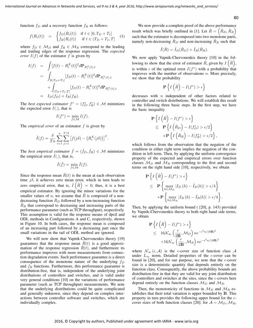
80



function fD and a recovery function fR as follows:

f(Ri(t)) =

{fD(Ri(t)) if t ∈ [0, TD + TI ]

fR(Ri(t)) if t ∈ (TD + TI , T ](1)

where fD ∈ MD and fR ∈ MR correspond to the leadingand trailing edges of the response regression. The expectederror I(f) of the estimator f is given by

I(f) =

∫[f(t)−RXi (t)]2dPRX

i (t),t

=

∫[0,TD+TI ]

[fD(t)−RXi (t)]2dPRXi (t),t

+

∫(TD+TI ,T ]

[fD(t)−RXi (t)]2dPRXi (t),t

= ID(fD) + IR(fR).

The best expected estimator f∗ = (f∗D, f∗R) ∈ M minimizes

the expected error I(.), that is

I(f∗) = minf∈M

I(f).

The empirical error of an estimator f is given by

I(f) =δ

Tn

n∑i=1

T/δ∑j=1

[f(jδ)−

(RXi (jδ)

)]2.

The best empirical estimator f = (fD, fR) ∈ M minimizesthe empirical error I(.), that is,

I(f) = minf∈M

I(f).

Since the response mean R(t) is the mean at each observationtime jδ, it achieves zero mean error, which in turn leads tozero empirical error, that is, I

(R)

= 0; thus, it is a bestempirical estimator. By ignoring the minor variations for thesmaller values of n, we assume that R is composed of a non-decreasing function RD followed by a non-increasing functionRR that correspond to decreasing and increasing parts of theperformance parameter (such as TCP throughput), respectively.This assumption is valid for the response means of dpctl andODL methods in Configurations A and C, respectively, shownin Figure 10. In both cases, the response mean is composedof an increasing part followed by a decreasing part once thesmall variations in the tail of ODL method are ignored.

We will now show that Vapnik-Chervonenkis theory [19]guarantees that the response mean R(t) is a good approxi-mation of the response regression R(t), and furthermore itsperformance improves with more measurements from connec-tion degradation events. Such performance guarantee is a directconsequence of the monotone nature of the underlying fDand fR functions. Furthermore, this performance guarantee isdistribution-free, that is, independent of the underlying jointdistributions of controllers and switches, and is valid undervery general conditions [10] on the variations of performanceparameter (such as TCP throughput) measurements. We notethat the underlying distributions could be quite complicatedand generally unknown, since they depend on complex inter-actions between controller software and switches, which areindividually complex.

We now provide a complete proof of the above performanceresult which was briefly outlined in [1]. Let R =

(RD, RR

)such that the estimator is decomposed into two monotone parts,namely non-decreasing RD and non-increasing RR such that

I(R) = ID(RD) + IR(RR).

We now apply Vapnik-Chervonenkis theory [10] in the fol-lowing to show that the error of estimator R, given by I

(R)

,is within ε of the optimal error I(f∗) with a probability thatimproves with the number of observations n. More precisely,we show that the probability

P{I(R)− I(f∗) > ε

}decreases with n independent of other factors related tocontroller and switch distributions. We will establish this resultin the following three basic steps. In the first step, we havethe basic inequality

P{I(R)− I(f∗) > ε

}≤ P

{I(RD

)− I(f∗D) > ε/2

}+P

{I(RR

)− I(f∗R) > ε/2

},

which follows from the observation that the negation of thecondition in either right term implies the negation of the con-dition in left term. Then, by applying the uniform convergenceproperty of the expected and empirical errors over functionclasses MD and MR corresponding to the first and secondterms on the right hand side [10], respectively, we obtain

P{I(R)− I(f∗) > ε

}≤ P

{maxh∈MD

|ID (h)− ID(h)| > ε/4

}+P

{maxh∈MR

|IR (h)− IR(h)| > ε/4

}.

Then, by applying the uniform bound ( [20], p. 143) providedby Vapnik-Chervonenkis theory to both right hand side terms,we obtain

P{I(R)− I(f∗) > ε

}≤ 16N∞

( ε

2B,MD

)ne−ε

2n/(8B)2

+16N∞( ε

2B,MR

)ne−ε

2n/(8B)2

where N∞ (ε,A) is the ε-cover size of function class Aunder L∞ norm. Detailed properties of the ε-cover can befound in [20], and for our purpose, we note that the ε-coversize is a deterministic quantity that depends entirely on thefunction class. Consequently, the above probability bounds aredistribution-free in that they are valid for any joint distributionof controllers and switches at the sites, since the ε-covers heredepend entirely on the function classes MD and MR.

Then, the monotonicity of functions in MD and MR es-tablishes that their total variation is upper bounded by B. Thisproperty in turn provides the following upper bound for the ε-cover sizes of both function classes [20]: for A =MD,MR,

81



we have

N∞( ε

2B,A)< 2

(4n

ε2

)(1+2B/ε) log2(2ε/B)

.

By using this bound, we obtain

P{I(Ri

)− I(f∗) > ε

}< 64

(4n

ε2

)(1+2B/ε) log2(2ε/B)

ne−ε2n/(8B)2 .

This bound provides qualitative insights into this approachwhen “sufficient” number of measurements are available. Theexponential term on the right hand side decays faster in n thanthe growth in other terms, and hence for sufficiently largen it can be made smaller than a given probability α. Thus,the expected error I(R) of the response mean used in theprevious section is within ε of the optimal error I(f∗) witha probability that increases with the number of observations,and is independent of the underlying distributions. An indirectevidence of this artifact is noticed in the increased stability ofthe response mean as we increase the number of connectiondegradation events from 10 to 100 in Figures 9(a) and 10,respectively.

The above probability estimates are not necessarily verytight in part due to the distribution-free nature of the per-formance guarantee. Nevertheless, this analysis provides asound statistical basis for using the response mean R as anapproximation to the underlying response regression R forcomparing different controllers and configurations.

VI. CONCLUSIONS

We considered scenarios with two sites connected overa dedicated, long-haul connection, which must fail-over to astandby connection upon degradations that affect the host-to-host application performance. Current solutions require sig-nificant customizations due to the vendor-specific softwareof network devices and applications, which often have to berepeated with upgrades and changes. Our objective is to exploitthe recent network virtualization technologies to develop fasterand more flexible software fail-over solutions. The presenceof a single long-haul connection and application-level triggersin these scenarios necessitate a solution that is different fromusual single controller methods commonly used in many SDNsolutions.

We first presented a light-weight method that utilizes hostscripts to monitor the connection rtt and dpctl API to imple-ment the fail-over. We then presented a second method usingtwo OpenDaylight (ODL) controllers and REST interfaces.We performed experiments using a testbed consisting of HPand Cisco switches connected over long-haul connectionsemulated in hardware by ANUE devices. They show that bothmethods restore TCP throughput, but their comparison wascomplicated by the restoration dynamics of TCP throughputwhich contained significant statistical variations. To accountfor them, we developed the impulse-response method basedon statistical finite-sample theory to estimate the responseregressions. It enabled us to compare these methods underdifferent configurations, and conclude that on the average thedpctl method restores TCP throughput several seconds fasterthan the ODL method.

It would be of future interest to generalize the proposedmethods to trigger fail-overs based on parameters of morecomplex client-server applications that utilize TCP for reliabledelivery. The performance analysis of such methods will likelybe much more complicated since the application dynamics maybe modulated by the already complicated TCP recovery dy-namics. Our test results are based on using CUBIC congestioncontrol mechanism [18] which is the default on Linux systems,and it would of future interest to test the performance of othercongestion control mechanisms, including high-performanceversions for long-haul [21] and satellite [22] connections.

Currently there seems to be an explosive growth in thevariety of SDN controllers including open source products,such as Helium, Lithium and Beryllium versions of ODL,Floodlight [23], ONOS [24] Ryu [25] and others, and alsovendor specific products and adaptations. Furthermore, thereis a wide variety of implementations of OpenFlow standardsby switch vendors, ranging from building additional softwarelayers on existing products to developing completely nativeimplementations. It would be of future interest to developgeneral performance analysis methods that enable us to com-pare various SDN solutions (that comprise of controllers,switches, docker containers and application modules) for morecomplex scenarios such as data centers and cloud servicesdistributed across wide-area networks. In particular, it wouldbe of interest to develop methods that directly estimate theperformance differences between different configurations frommeasurements using methods such as the differential regressionmethod [26].

It would be of future interest to generalize the approachof this paper to develop a baseline test harness wherein acontroller or a switch can be plugged into a known, fixedconfiguration. The general approach is to develop canonicalconfigurations each with fixed components of the harness, suchas application trigger modules, physical network connectionsand others. Then, impulses responses of different controllers,switches or other SDN components can be generated in theseconfigurations, and they can be objectively compared to assesstheir relative performance.

ACKNOWLEDGMENTS

This work is funded by the High-Performance Networking Pro-gram and the Applied Mathematics Program, Office of AdvancedComputing Research, U.S. Department of Energy, and by ExtremeScale Systems Center, sponsored by U. S. Department of Defense,and performed at Oak Ridge National Laboratory managed by UT-Battelle, LLC for U.S. Department of Energy under Contract No.DE-AC05-00OR22725.

REFERENCES[1] N. S. V. Rao, “Performance comparison of SDN solutions for switching

dedicated long-haul connections,” in Proceedings of International Sym-posium on Advances in Software Defined Networking and NetworkFunctions Virtualization, 2016.

[2] Y. D. Lin, D. Pitt, D. Hausheer, E. Johnson, and Y. B. Lin, “Software-defined networking: Standardization for cloud computing’s secondwave,” IEEE Computer: Guest Editorial, November 2014, pp. 19–21.

[3] D. Kreutz, F. M. V. Ramos, P. E. Verissimo, C. E. Rothenberg,S. Azodolmolky, and S. Uhlig, “Software-defined networking: A com-prehensive survey,” Proceedings of the IEEE, vol. 103, no. 1, 2015, pp.14–76.

[4] W. Xia, Y. Wen, C. H. Foh, D. Niyato, and H. Xie, “A surveyon software-defined networking,” IEEE Communication Surveys &Tutorials, vol. 17, no. 1, First Quarter 2015, pp. 27–51.

82



[5] T. D. Nadeau and K. Gray, Software Defined Networks. OReillypublishers, 2013.

[6] “Opendaylight.” [Online]. Available: www.opendaylight.org[7] Y. Srikant, The Mathematics of Internet Congestion Control.

Birkhauser, Boston, 2004.[8] W. R. Stevens, TCP/IP Illustrated. Addison Wesley, 1994, volumes

1-3.[9] N. S. V. Rao, J. Gao, and L. O. Chua, “On dynamics of transport

protocols in wide-area internet connections,” in Complex Dynamics inCommunication Networks, L. Kocarev and G. Vattay, Eds. Springer-Verlag Publishers, 2005.

[10] V. N. Vapnik, Statistical Learning Theory. New York: John-Wiley andSons, 1998.

[11] N. S. V. Rao, W. R. Wing, , S. M. Carter, and Q. Wu, “Ultrasciencenet: Network testbed for large-scale science applications,” IEEE Com-munications Magazine, vol. 43, no. 11, 2005, pp. s12–s17.

[12] J. Tourrilhes, P. Sharma, S. Banerjee, and J. Pettit, “SDN and OpenFlowevoltion: A standards perspecitve,” IEEE Computer, November 2014,pp. 22–29.

[13] C. E. Rothenberg, R. Chua, J. Bailey, M. Winter, C. N. A. Correa, S. C.de Lucena, M. R. Salvador, and T. D. Nadeau, “When open source meetsnetwork control planes,” IEEE Computer, November 2014, pp. 46–53.

[14] N. S. V. Rao, S. E. Hicks, S. W. Poole, and P. Newman, “Testbedand experiments for high-performance networking,” in Tridentcom:International Conference on Testbeds and Research Infrastructures forthe Development of Networks and Communities, 2010.

[15] “Open networks foundation.” [Online]. Available: www.opennetworking.org

[16] “Software defined networks,” cisco Systems. [Online]. Available:www.cisco.com

[17] “Software defined networking,” hP. [Online]. Available: www.hp.com[18] I. Rhee and L. Xu, “Cubic: A new tcp-friendly high-speed tcp variant,”

in Proceedings of the Third International Workshop on Protocols forFast Long-Distance Networks, 2005.

[19] V. N. Vapnik, The Nature of Statistical Learning Theory. New York:Springer-Verlag, 1995.

[20] M. Anthony and P. L. Bartlett, Neural Network Learning: TheoreticalFoundations. Cambridge University Press, 1999.

[21] T. Yee, D. Leith, and R. Shorten, “Experimental evaluation of high-speed congestion control protocols,” Transactions on Networking,vol. 15, no. 5, 2007, pp. 1109–1122.

[22] J. Cloud, D. Leith, and M. Medard, “Network coded tcp (ctcp) perfor-mance over satellite networks,” in SPACOMM 2014, 2014.

[23] “Project floodlight.” [Online]. Available: www.projectfloodlight.org[24] “Onos overview.” [Online]. Available: www.onosproject.org[25] “Build SDN agilely.” [Online]. Available: osrg.github.io/ryu/index.html[26] B. W. Settlemyer, N. S. V. Rao, S. W. Poole, S. W. Hodson, S. E.

Hicks, and P. M. Newman, “Experimental analysis of 10gbps transfersover physical and emulated dedicated connections,” in InternationalConference on Computing, Networking and Communications, 2012.

83



A Model for Managed Elements under Autonomic Cloud Computing Management

Rafael de Souza Mendes∗, Rafael Brundo Uriarte†, Carlos Becker Westphall∗∗Federal University of Santa Catarina, Florianopolis, Brazil

emails: [email protected], [email protected]†IMT School for Advanced Studies Lucca, Italy

email: [email protected]

Abstract—Due to the scale and dynamism of cloud computing,there is a need for new tools and techniques for its management.This paper proposes an approach to quantitative modelling ofcloud components’ behaviour, using double weighted DirectedAcyclic Multigraphs (DAM) through the different abstractionlevels of components. With this formalism, it is possible to analyseload propagation and its effects on the cloud elements from anAnything as a Service (xAAS) perspective. Such model enablesthe comparison, analysis and simulation of clouds, which assistthe cloud management with the evaluation of modifications inthe cloud structure and configuration. The existing solutionseither do not have mathematical background, which hindersthe comparison and production of structural variations in cloudmodels, or have the mathematical background, but are limitedto a specific area (e.g., energy-efficiency), which does not providesupport to the dynamic nature of clouds and to the different needsof the managers. In contrast, our model has a formal math-ematical background and is generic. Furthermore, we presentformalisms and algorithms that support the load propagationand the metrics of services, systems, third-parties providers andresources, such as: computing, storage and networking. To demon-strate the applicability of our solution, we have implemented asoftware framework for modelling Infrastructure as a Service,and conducted numerical experiments with hypothetical loadsand behaviours.

Keywords-Autonomic Cloud Computing; Cloud ComputingManagement; Simulation; Multigraph.

I. INTRODUCTIONThe management of pooled resources according to high-

level policies is a central requirement of the as a servicemodel, as fostered by Cloud Computing (CC). The two majorfunctions in CC management, planning and decision making,are challenging and are still an open issues in the field. In ourprevious work [1], we have presented a formal model, basedon Direct Acyclic Multigraphs (DAM) [2], to model the cloudelements’ behaviour regarding loads and evaluations. Thisformal model intents to reduce the gap between AutonomicCC [3], [4] management and well-established approaches indecision theory [5] and managerial science [6]. In this regard,was presented a managed elements model which make easierthe inference of states, actions and consequences. These states,actions and consequences are the bases for planning modelsand the core of our proposal to fulfil the lack between CC anddecision methods. This lack of formal models is highlightedby our previous efforts to develop methods for CC autonomicmanagement: [4][7][8] and formalisms based on Service LevelAgreement (SLA) [9].

Currently, the existing solutions which provide CC models

can be classified into two main groups: general models, usuallyrepresented by simulators; and specific models, devised fora particular field (e.g., energy saving). The former lacksa mathematical formalisation that enables comparisons withvariations on the modellings. The latter usually have the formalmathematical background but, since they are specific, they donot support reasoning on different management criteria andencompass only cloud elements related to the target area.

The main obstacle to establish formal general models isto express the conversion of loads from abstract elements(i.e., services or systems) to their concrete components (i.e.,physical machines or third-party services). However, suchmodel is mandatory to simulate and analyse qualitatively andquantitatively the CC elements’ behaviour, which facilitate theevaluation of managerial decisions, especially if the modeldeals with abstraction and composition of these elements.The need of this model do express managerial knowledgeincreases as concept of CC moves away from the conceptof infrastructure and Anything as a Service (xAAS) providersbuild high level cloud structures. To address this gap in theliterature, we analyse the domain elements and characteristicsto propose the Cloud Computing Load Propagation (C2LP)graph-based model, which is a formal schema to express theload flow through the cloud computing components, and theload’s impact on them. This schema is required because thesystem analysis is performed in design time and focus on thebehaviour of data when passing through the cloud structures,however, the cloud management requires a view about thebehaviour of the structures when the loads are passing throughthem, in runtime. Therefore, we define a load as the type andamount of effort to process services’ requests in systems orresources.

For example, the (C2LP) model enables the comparison ofdifferent cloud structures, the distinction of load bottlenecks,the expression of conversion of loads units (change in type)between elements, the quantitative analysis of the load prop-agation and the evaluation of the effects of processing a loadon the cloud structure. In more general terms, such solutionunifies heterogeneous abstraction levels of managed elementsinto a single model and can assist the decision-making tasksin processes, such as: load balance, resource allocation, scaleup/down and migrations. Moreover, simulations performedusing our model can be useful to predict the consequencesof managerial decisions and external events, as well as theevolution of baseline behaviour, in several abstraction levels.

More specifically, we model the basic components of CC:

84



(i) services; (ii) systems; (iii) resources, in which systems aredeployed, that can be computing, storage and networking; and(iv) third-party clouds that deploy services. This taxonomy per-mits putting together, based on Directed Acyclic Multigraphs,the CC elements on different abstraction levels. It enablesthe manager to access consolidated graph analytical toolsto, e.g., measure the components interdependencies, which isused to improve the availability and resource allocation. Inorder to demonstrate the applicability and advantages of theC2LPmodel, we present a use case where our model is usedto compare and evaluate different managerial configurationsover several quantitative behaviour in load propagation andevaluation.

This article is organised as follows. Section II discusses theexisting cloud models, the works that inspired the definitionof this model and the background information necessary forthe appreciation of this work. In Section III, we present anoverview of the model, formalise it, the propagation algorithm,and the evaluation process. Section IV describes the implemen-tation and the analysis performed on a use case. Finally, inSection V, we discuss the limitations and the future directionsfor the research.

II. RELATED WORKThis section presents the related works that propose models

to describe and simulate clouds. We have analysed them froma cloud provider management perspective, considering theircapacity to: express general cloud models, define componentsof the managed cloud instance; compare structures; simulatebehaviours and provide formal specifications with mathemati-cal background. Table I summarises model’s comparisons andthe discussion about the survey is presented as follows.

We grouped the proposals into two classes: general andspecific. General models, such as CloudSim [10], GreenCloud[12], iCanCloud [14], EMUSIM [15] and MDCSim [17], areusually associated with simulators and used to evaluate severalcriteria at the same time. On the other hand, specific models arecommonly associated with particular criterion evaluation, suchas performance [18], security [20][21], accounting [22][23] orenergy [24].

CloudSim [10] was originally built on top of GridSim[11] and focus on modelling data centres. Its framework isJava based and loads are modelled through a class called“CloudLet”, or an extension of it. Depiste its popularity,CloudSim does not have a strong mathematical background.This lack of formalism hinders the investigation of data cross-ing between states and configuration parameter, which limitthe exploration of the cloud behaviours. Furthermore, the coreclasses of CloudSim model data centre elements as: physicalmachines, virtual machines (VMs), networks and storages; andrequires customisations to deal with more abstract elements,e.g., services. Finally, also the comparison of simulation struc-tures is not straightforward with CloudSim.

Kliazovich et al. in [12] presented GreenCloud, an exten-sion of the network simulator NS2 [13] that offers a fine-grained modelling of the energy consumed by the elementsof the data centre, such as servers, switches, and links. Green-Cloud is a programmatic framework based in C++ and TCLscripts that, despite having the statistic background of NS2,does not have itself an underlying mathematical formalism.It also focuses on the data centres view and need extensionsto consider abstract elements as services and systems. Even

though the authors provided a comparison between data centrearchitecture in [12], the model does not favor the comparisonof simulation structures.

The simulator iCanCloud, presented in [14], is also a gen-eral data centre simulation tool. Based in C++, it has classesas “Hypervisor”, “Scheduler” and “VM” in the core classstructure, which demonstrates its high level of coupling withinfrastructure. Although the authors proposed iCanCloud as“targeted to conduct large experiments”, it does not offer nativesupport to compare structural changes between simulations. Asthe other general simulator, iCanCloud lacks of mathematicalformalisms.

EMUSIM [15] is an emulator and simulator that enables theextraction of information from the application behaviour – viaemulation – and uses the information to generate a simulationmodel. The EMUSIM has been built on top of two frameworks:Automated Emulation Framework (AEF) [16] (an emulationtestbed for grid applications) and CloudSim [10]. The objectiveof EMUSIM understand application’ behaviour profiles, toproduce more accurate simulations and, consequently, to adaptthe Quality of Service (QoS) and the budget required forhosting the application in the Cloud. Although EMUSIMpartially addresses the lack of capacity to model applicationof CloudSim, adding higher level modelling layer, it still lacksmathematical formalisms as well as the support to comparesimulation structures.

Finally, MDCSim presents a multi-tier data centre sim-ulation platform. However, this multi-tier modelling workswith concrete elements, in resource level, as a front-endtier/web server, a mid tier/application server, and a back-end tier/database server. The MDCSim also works with somemetrics in a higher abstraction level on specific Java elementsas EJBs and Tomcat. This approach still lacks a representationfor abstract elements, such as services and systems, wheremetrics and parameters are related to groups of elements (e.g.,availability of a service depending on several elements).

Overall, works proposing general models are data centre fo-cused and have evolved from Grid Computing, which may hin-ders their usage on service orchestration level and with third-parties cloud infrastructures, where data centre concepts arenot applicable. Designers of autonomic management methodsrequire the generation of cloud architectures and behaviours ina combinatorial fashion, in order to test plans, decisions andconsequences on a wide number cloud architectures, featuresthat not supported in these models.

In the second group of proposals, that is, frameworksdevised for a specific area, in-depth analysis based on robustformalisms are usually provided, such as queue theory [24][18], probability [20], fuzzy uncertainty [23] and heuristics[22]. However, their models do not fit well in integratedmanagement methods that intend to find optimal configurationsconsidering several criteria of distinct types. Moreover, specificoptimisation models are usually sensible to structural changes,having no robustness to support the dynamic nature of theclouds.

Vilaplana et al. in [18] presented a queue theoretic mod-elling for performance optimisation for scale CC. The modelhas a strong mathematical background and is able to evaluatejobs and VM scheduling policies using simulations. Never-theless, this optimisation is dependent on strong assumptions,i.e., that the back-end tier is modelled as an Open Jacksonnetwork [19]. The model is focused on evaluation and it is

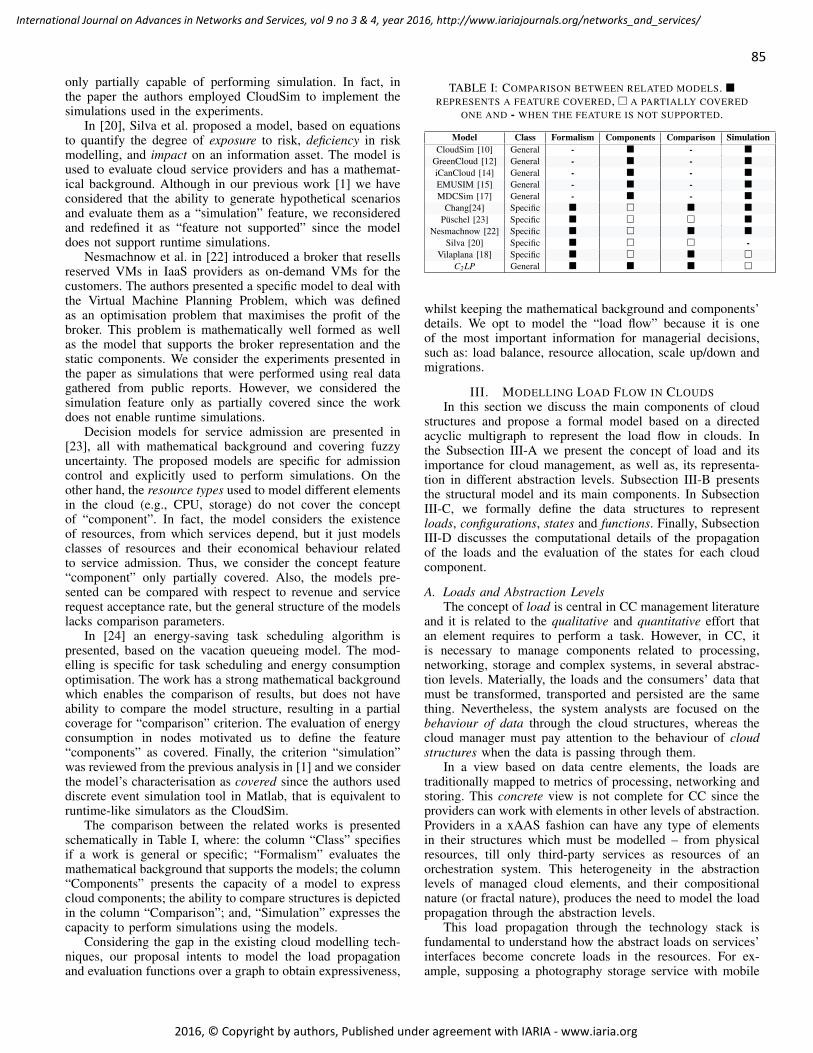
85



only partially capable of performing simulation. In fact, inthe paper the authors employed CloudSim to implement thesimulations used in the experiments.

In [20], Silva et al. proposed a model, based on equationsto quantify the degree of exposure to risk, deficiency in riskmodelling, and impact on an information asset. The model isused to evaluate cloud service providers and has a mathemat-ical background. Although in our previous work [1] we haveconsidered that the ability to generate hypothetical scenariosand evaluate them as a “simulation” feature, we reconsideredand redefined it as “feature not supported” since the modeldoes not support runtime simulations.

Nesmachnow et al. in [22] introduced a broker that resellsreserved VMs in IaaS providers as on-demand VMs for thecustomers. The authors presented a specific model to deal withthe Virtual Machine Planning Problem, which was definedas an optimisation problem that maximises the profit of thebroker. This problem is mathematically well formed as wellas the model that supports the broker representation and thestatic components. We consider the experiments presented inthe paper as simulations that were performed using real datagathered from public reports. However, we considered thesimulation feature only as partially covered since the workdoes not enable runtime simulations.

Decision models for service admission are presented in[23], all with mathematical background and covering fuzzyuncertainty. The proposed models are specific for admissioncontrol and explicitly used to perform simulations. On theother hand, the resource types used to model different elementsin the cloud (e.g., CPU, storage) do not cover the conceptof “component”. In fact, the model considers the existenceof resources, from which services depend, but it just modelsclasses of resources and their economical behaviour relatedto service admission. Thus, we consider the concept feature“component” only partially covered. Also, the models pre-sented can be compared with respect to revenue and servicerequest acceptance rate, but the general structure of the modelslacks comparison parameters.

In [24] an energy-saving task scheduling algorithm ispresented, based on the vacation queueing model. The mod-elling is specific for task scheduling and energy consumptionoptimisation. The work has a strong mathematical backgroundwhich enables the comparison of results, but does not haveability to compare the model structure, resulting in a partialcoverage for “comparison” criterion. The evaluation of energyconsumption in nodes motivated us to define the feature“components” as covered. Finally, the criterion “simulation”was reviewed from the previous analysis in [1] and we considerthe model’s characterisation as covered since the authors useddiscrete event simulation tool in Matlab, that is equivalent toruntime-like simulators as the CloudSim.

The comparison between the related works is presentedschematically in Table I, where: the column “Class” specifiesif a work is general or specific; “Formalism” evaluates themathematical background that supports the models; the column“Components” presents the capacity of a model to expresscloud components; the ability to compare structures is depictedin the column “Comparison”; and, “Simulation” expresses thecapacity to perform simulations using the models.

Considering the gap in the existing cloud modelling tech-niques, our proposal intents to model the load propagationand evaluation functions over a graph to obtain expressiveness,

TABLE I: COMPARISON BETWEEN RELATED MODELS. �REPRESENTS A FEATURE COVERED, � A PARTIALLY COVERED

ONE AND - WHEN THE FEATURE IS NOT SUPPORTED.

Model Class Formalism Components Comparison SimulationCloudSim [10] General - � - �

GreenCloud [12] General - � - �iCanCloud [14] General - � - �EMUSIM [15] General - � - �MDCSim [17] General - � - �

Chang[24] Specific � � � �Puschel [23] Specific � � � �

Nesmachnow [22] Specific � � � �Silva [20] Specific � � � -

Vilaplana [18] Specific � � � �C2LP General � � � �

whilst keeping the mathematical background and components’details. We opt to model the “load flow” because it is oneof the most important information for managerial decisions,such as: load balance, resource allocation, scale up/down andmigrations.

III. MODELLING LOAD FLOW IN CLOUDSIn this section we discuss the main components of cloud

structures and propose a formal model based on a directedacyclic multigraph to represent the load flow in clouds. Inthe Subsection III-A we present the concept of load and itsimportance for cloud management, as well as, its representa-tion in different abstraction levels. Subsection III-B presentsthe structural model and its main components. In SubsectionIII-C, we formally define the data structures to representloads, configurations, states and functions. Finally, SubsectionIII-D discusses the computational details of the propagationof the loads and the evaluation of the states for each cloudcomponent.

A. Loads and Abstraction LevelsThe concept of load is central in CC management literature

and it is related to the qualitative and quantitative effort thatan element requires to perform a task. However, in CC, itis necessary to manage components related to processing,networking, storage and complex systems, in several abstrac-tion levels. Materially, the loads and the consumers’ data thatmust be transformed, transported and persisted are the samething. Nevertheless, the system analysts are focused on thebehaviour of data through the cloud structures, whereas thecloud manager must pay attention to the behaviour of cloudstructures when the data is passing through them.

In a view based on data centre elements, the loads aretraditionally mapped to metrics of processing, networking andstoring. This concrete view is not complete for CC since theproviders can work with elements in other levels of abstraction.Providers in a xAAS fashion can have any type of elementsin their structures which must be modelled – from physicalresources, till only third-party services as resources of anorchestration system. This heterogeneity in the abstractionlevels of managed cloud elements, and their compositionalnature (or fractal nature), produces the need to model the loadpropagation through the abstraction levels.

This load propagation through the technology stack isfundamental to understand how the abstract loads on services’interfaces become concrete loads in the resources. For ex-ample, supposing a photography storage service with mobile

86



and web interfaces, the upload of an array of photos canrepresent a load in the server-side interface (expressed innumber of photos), whereas, the same load must be expressedin several loads on (virtual) links, (virtual) processors, and(virtual) storages, not necessarily related to time. In fact, theupload of an array of photos is an abstract load and can be anuseful to perform billing metrics, but it can be not useful tomeasure performance, requiring the detailing to concrete loads,according to the cloud’s service implementation. An autonomicmanager agent, responsible for planning and decision makingin runtime, must understand the quantitative relations into themanaged cloud structure to work in real time.

Thus, using a graph to express the dependences betweenelements in different levels, the abstracter elements (services’interface) must appear in the roots of the graph, the con-creter elements (resources) must appear in the leaves, whereasthe intermediary elements (systems) orchestrate resources inorder to implement the services. These concepts of servicesinterfaces, systems and resources become relative terms whichcan adapted for any cloud implementation, independent ofabsolute level of operation regards to the IaaS, PaaS and SaaStaxonomy.

B. Modelling Clouds with C2LPIn C2LP, the structural arrangement of cloud elements

is based in a directed acyclic multigraph (DAM) where thenodes of the graph represent components. To start a horizontaldecomposition must be considered the four main types for CCelements:• Resources are the base of any cloud, and can be clas-

sified in three elementary computational function: asComputing, Storage and Networking; Therefore, thesecomponents are always leaf nodes, even when virtualizedor based on service orchestration (e.g., a storage blockdevice built on email accounts). The elements with thesecomputational functions constitute the sources of comput-ing power into a cloud. The term “computing power” isused here not only for processing, but also for networkingand storage, since the CC paradigm effectively offer theselast as services, exposing their economical value.

• Systems are abstractions of orchestrated resources thatimplement services. They can be, e.g., applications andplatforms. In the model, systems must be directly linkedto at least one of each type of resource: computing, stor-age and networking. Nevertheless, these resources mightbe replaced by other systems or third-party services. Insuch cases, the relationship between the system and theelement that represents the resource (e.g., another systemor the third-party service) must be explicitly definedusing stereotypes (virtual computing, virtual networkingor virtual storage).

• Third-Party Services represent: (i) resources to systemcomponents, when the relation is explicitly annotated withthe appropriated stereotype, and (ii) entire systems whichprovide services and abstract the underlying layers (e.g.,email services). The latter models, for example, hybridclouds or composed services.

• Services are interfaces between the cloud and the con-sumers. They must be connected with a respective systemthat implement them and never are directly linked toresource or third-party services. Services interfaces arethe points on which the specification of the consumer’s

needs (SLAs) are attached. In your model the servicesinterfaces can receive loads from a hypothetical commonsource (*), that symbolizes the consumer.

Directed edges define to which elements each cloud com-ponent can transmit load. Nodes have two main processes:propagation of the load; and evaluation of the impact of theload in the node itself. Remarkably, the resources componentsdo not propagate load and are the only nodes that actuallyrun the assigned load, while other elements are abstract (e.g.,applications, middlewares, platforms and operations systems).Moreover, we consider in the model also the configurationssettings of nodes, which impact the propagation and evaluationprocesses.

Providers offers services and receive requests from con-sumers. These request represent an economical demand bywork, which in providers’ assets represent workloads, or just:loads. The loads vary according to each cloud component andare changing in quality and quantity along the computing chainthat compose the providers’ assets. Therefore, each node in theDAM represents a function that convert the input load to outputload, from the services (sources) to the resources (sinks). In theresources occurs the work, realizing the load and consumingcomputing power.

In fact, just low abstraction loads would need to berepresented in the model, e.g., supposing an IaaS provider:link, processor and storage. However, the patterns of be-haviour in low level loads become chaotic and unmanageablewithout information about the abstract component that guidethe resources usage. Therefore, distributing load propagationfunctions over a graph is a simple way to represent complexfunction compositions on a conceptual network. Assumingthat the loads flow from the sources (services) to the sinks(resources), and a node must have all incoming loads availableto compute the outgoing loads, the propagation must be madein a breadth-first fashion.

Since loads might have different forms, we model theserelations enabling multiple edges between nodes, which sim-plifies the understanding of the model. For example, a ser-vice transmits 10 giga FLoating-point Operations Per Second(FLOPS) and 100 giga bytes of data to third-party service.This case is modelled using two edges, one for each type ofload to the third-party. In case of change in the structure (e.g.,the executor of the loads finds a cheaper storage provider)the model can be adjusted simply by removing the storageedge between these nodes and adding it to this new third-partyprovider.

When the loads are realized in the resources, they produceseveral effects which can be measured by the monitoring. Forexample: resource usage, energy consumption, fails, costs, etc.The modelling of qualitative and quantitative relations betweenloads and their effects over the resource is a mandatory taskto enable managerial planning and decision making. Neverthe-less, measurable effects in resources can also signify metrics insystem and services. For example, the sum of energy consumedin the processors, network and storage, in order to downloada photo of 10GB, means the amount of energy consume doresolve a load of type “download photo” of size “10GB”, inservice level.

However, is not only the loads which determine thebehaviours of the resources, but also the configurationparametrized by the cloud manager, and the accumulated ef-

87



fects from previous loads. On the other hand, non-leaf elements– which the evaluations depend of lower level elements – mustconsider: incoming loads, the accumulated state (a priori) andthe state of lower elements (target nodes). This is representedin the model as distinct evaluation functions. In the C2LP weremodelled a set of evaluated functions for leaf nodes, with twoinputs, and a set for non-leaf nodes, with three inputs. The bothtype of functions output a new node state which can containseveral sub-evaluations (measures).

The propagation of evaluations is done after the propaga-tion of loads, from bottom to top. This procedure will providethe amount of loads in each element of the model. With theloads and the configurations and accumulated state (a prioristate) in the resources elements, it is possible to compute thenew configurations and accumulated state (the a posterioristate). So, in the non-leaf nodes it is possible to computethe a posteriori state with its the a priori state and the aposteriori states of its dependencies (lower level elements). Toperform the evaluation of whole graph, from the root nodes,it is necessary to perform a depth-first computing though thegraph.

Figure 1 presents the modelling of a scenario, in which acloud provides two services: an email and Infrastructure-as-a-Service (IaaS). The IaaS is provided by a third-party cloud.The email service instead, employs a system component torepresent a software email server (in this case a Postfix). Thiscomponent uses local computing and networking and storagefrom a third-party cloud. The relation (edge) between thesecomponents is annotated accordingly.

In the proposed scenario, we exemplify the load propaga-tion with a request from consumers to send 2 new emails usingthe email service. These 2 emails are converted by the servicecomponent into 2 loads of type “transaction” and sent for theemail server where they are converted into another types ofload and propagated to the resources linked to the server.

The evaluation process of this scenario uses differentmetrics in each node and is marked as “eval:“. For example, inthe service level, the load of 2 emails was measured in termsfinancial cost and energy necessary to complete the request.

C. Formalisation of the ModelFormally, in C2LP model, a cloud C can be expressed as

C = (V,E, τV , σ,Φ, φ,Γ, γ,Γ′, γ′), where:• V is the set of nodes V = {v1, v2, . . . , vn} of the

multigraph, such that every item in V represents oneelement of the cloud and has one respective node-weightwv , that usually is a vector of values;

• E is the set of directed edges where E ={e1, e2, . . . , em}|e = (v, v′), that describes the ability ofa source node v to transmit a load to node v′, such thateach em also has a respective edge-weight wv,v′ ;

• τV : V → TV is a bijective function whichmaps the nodes with the respective type, wherethe set TV is the set of types of nodes, suchthat TV = {′computing′, ′storage′, ′networking′,′system′, ′service′, ′third party′};

• σ : E{→system,→third−party} → {none, vComputing,vStorage, vNetworking} is a function which maps theedges that have systems and third-party services as targetwith the respective stereotype, characterising the relationbetween the source element with the target;

• Φ represents the set of propagation functions, where

NetworkingComputing

Third-partyIaaS

Consumers

EmailService

PostfixServer

Third-party

Cloud

load: 2 New Emails

load: 2 Transactions

load: 1 gFLOP

load: 2.5mbload: 20 kb

<v-Storage>

eval:(2 kw,10 sec)

eval:(0.3 Euros)

eval:(1 kw)

eval: (3 kw, 0.8 Euros)

eval: (3 kw, 0.8 Euros)

load: 2 mb

IaaS

Figure 1: Example of the propagation of loads and the evaluationprocesses using the C2LP model.

Φ = {f1, f2, . . . , fv} and φ is a bijective functionφ : V → Φ that maps each node for the respectivepropagation function. Each function in the set Φ is definedas fv : Nn,Ri → Ro, where: the set Nn representsthe space where the n-tuple for the configuration iscontained; the set Ri represents the space where the n-tuple of incoming edge-weights is contained; and, Ro isthe space where the n-tuple of the outgoing edge-weightsis contained. To simplify the model and the algorithms,we consider that configurations are stored in the node-weight, such that wconf

v represents the configuration partof the node-weight vector.

• Γ is the set of sets that contains the evaluation functionsfor the leaf nodes, such that there exists one functionfor each distinct evaluation metric (e.g., energy use,CO2 emission, . . . ). Then, Γ = {Γ1,Γ2, . . .Γk}, suchthat Γk = {gn+1, gn+2, . . . , gm}. Each set Γk is re-lated to a leaf node v ∈ V[leaf ] through the bijectivefunction γ : V[leaf ] → Γ. Every gn+m is stored ina distinct position of the node-weight vector of therespective node – representing a partial state of v –such that the full new state can be computed throughthe expression: w′v = (c1, . . . , cn, gn+1(c1, . . . , cn, w

iv),

gn+2(c1, . . . , cn, wiv), . . . , gn+m(c1, . . . , cn, w

iv)), where:

c1, . . . , cn is the n-tuple with the configuration part ofthe node-weight wv; wi

v is the n-tuple with all incomingedge-weights w∗,v of v; and w′v is the new node-weight(full state) for v. The complete evaluation procedure isdetailed in Figure 6;

• Γ′ is the set of sets that holds the evaluation functionsfor non-leaf nodes. Therefore, Γ′ = {Γ′1,Γ′2, . . . ,Γ′l},such that each set Γ′l = {g′n+1, g

′n+2, . . . , g

′m} con-

tains the evaluation functions g′n+m. Every Γ′l is as-sociated with a non-leaf node v through the bijective

88



edge-weight edge-weight edge-weight edge-weight

(node-weight)

f(...)


Figure 2: Illustration of load propagation in root or non-leaf nodes.

function γ′ : Vnon−leaf → Γ′. Since the result ofeach function g′n+m is stored in a distinct positionof w′v , it represents a partial state of the respectivenode v. A new full state of non-leaf nodes can becomputed through the expression: w′v = (c1, . . . , cn,g′n+1(c1, . . . , cn, w

iv, w

′uv

), g′n+2(c1, . . . , cn, wiv, w

′uv

),. . . , g′n+m(c1, . . . , cn, w

iv, w

′uv

)); where w′v is the newnode-weight of v, c1, . . . , cn is the n-tuple with theconfiguration part wconf

v of the node-weight, wiv is the

n-tuple with the incoming edge-weights e∗,v of v, andw′uv

is a tuple which puts together all node-weights ofthe successors of v (see Figure 6 for details).

The main objective of these formalisms is to specifythe data structures that support a model validation, the loadpropagation, and elements evaluations. The details of eachprocedure concerned with propagation and evaluations aredescribed in Subsection III-D.

D. Details on the Propagation and EvaluationThe load propagation consists in a top-down process that

uses the breadth-first approach. In a breadth-first algorithm,all the incoming loads are available for a node before theinference of its outgoing loads. In the specific case on C2LPthe algorithm starts from the loads on the services, correspond-ing to the requests received from consumers. The Figure 2illustrates the load propagation. The blue oblong represents anon-leaf element that has incoming edges, which the weightsrepresent incoming loads. Alto, there is the node-weight thatrepresents the a priori state, that contains the configurationsand accumulated states. Both, the incoming loads and node-weight, are used as inputs for the node attached propagationfunction f(...), that produces a tuple with the output edge-weights.

The propagation process uses a queue with the servicenodes (the roots of the graph). Then, a node v is pickedfrom this queue and all its children are placed into the queue.Afterwards, a function fv = φ(v) is executed to distribute theload, that is, to define all edge-weights for the outgoing edgesof v. This procedure is repeated while the queue is not empty.

1: procedure BREADHTFIRSTPROPAGATION(C,WV ,WE) .Requires a cloud model C = (V,E, τV , σ,Φ, φ), theset of node-weights WV |∀v ∈ V ∧ ∃!wv ∈ WV andthe set of edge-weights WE |∀ev,v′ ∈ E ∧ ∃!wv,v′ ∈WE .

2: queue← ∅3: enqueue(∗)4: repeat5: v ← dequeue()6: for each u ∈ successorSet(v) do7: enqueue(u)8: end for . enqueues the sucessor of each node9: fv ← φ(v)

10: wconfv ← configurationPart(wv) . gets the

config. part of the node-weight (state).11: wi

v ← (w1,v, w2,v, . . . , wu,v) . builds theincoming edge-weights in a tuple wi

v .12: wo

v ← fv(wconfv , wi

v) . wov contains the result of

the propagation function.13: for each wv,u ∈ wo

v do14: WE ←WE ⊕ wv,u . replaces the old value

of wv,u.15: end for. assign the values for the outgoing edges

of v.16: until queue 6= ∅

return WE

17: end procedure

Figure 3: Breadth-first algorithm used for the load propagation.

The well defined method is detailed in Figure 3.When the load is propagated to resources components (leaf

nodes), they execute the load. This execution requires powerand resources and can be evaluated in several forms. For exam-ple, energy (kw), performance, availability, accounting, secu-rity, CO2 emissions and other cloud specific feature units. Thisevaluation process takes every function gn+m ∈ Γk in orderand computes each partial states, storing them into a position ofthe new node-weight w′v . A finer description can be defined as:w′v = (wconf

v , gn+1(wconfv , wi

v), . . . , gn+m(wconfv , wi

v), suchthat w′v represents the a posteriori state for the node v, wconf

vare the configurations (a priori state) of v, wi

v are the incomingedge-weights of v, and gn+m ∈ γ(v) are the evaluationfunctions associated with the node.

The process of evaluation in leaf nodes is depicted in theFigure 4, where the pink oblong represents a leaf node. In thesenodes the edge-weights and the a priori node-weight serve asinputs for each function in the vector of evaluation functions,which produce a single value each one. These single values aregrouped in a tuple that results in the a posteriori node weight.

The evaluations also include the non-leaf nodes sincethe load also passes through them and it is useful, e.g., tounderstand the load distribution and to identify bottlenecks.In the case of non-leaf nodes, the evaluation requires also theevaluation results of the bottom nodes. Therefore, this processis performed from the leaves to the roots using a depth-firstapproach.

A non-leaf node receives the tuples (config, loads,children states), and evaluates by the processingof all g′n+m ∈ γ′(v) functions. A representation

89



(g(...),...,g(...))

(node-weight)

(node-weight')(node-weight')


Figure 4: Illustration of evaluations in leaf nodes.

of this process can be described as: w′v =(wconf

v , g′n+1(wconfv , wi

v, w′uv

), . . . , g′n+m(wconfv , wi

v, w′uv

),such that w′v represents the new node-weight (a posterioristate) for the node v, wconf

v are the configuration part (apriori state) of node-weight into v, wi

v represent the incomingedge-weights of v, w′uv

are the computed node-weights ofthe successors of v, and g′n+m ∈ γ′(v) are the evaluationfunctions associated with the node.

The evaluation in a non-leaf node is depicted in the Figure5, where the blue oblong represents a non-leaf. In this figure itis possible to observe the a posteriori node-weights from thelower level elements being “transmitted” through the edges.The proximity of node-weights with edges do not represent theassociation between them, but the transmission of one throughthe other. Into the node is depicted the vector of evaluationfunctions, which will receive: the a priori node-weight ofthe node itself and the a posteriori node-weights from thelower elements; and produce single values which are grouped,in order to compose a posteriori node-weight tuple for thenode itself. This a posteriori node-weight is propagated forthe upper elements through the edges. The node-weight in thesuperior edges have the same value, the computed a posteriorinode-weight, for all edges. Also, the arrows do not representthe direction of the edges, but the information flow.

The complete evaluation process is detailed in Figure 6,where a stack is used to perform a depth-first computation.The first non-visited child of a current node is placed into thestack and will be used as current node. When all children of anode are evaluated, then the node is evaluated. If the node is aleaf node the g functions are used to compute the evaluations,otherwise, the g′ functions are used instead.

These mathematical structures and algorithms provide ageneral framework for modelling and evaluation of clouds’elements behaviour in different abstraction levels. They canexpress and compute how service level loads are decomposedand converted, through the systems, till become resource levelloads. In resource level, on concrete elements, the loads canbe evaluated according to performance, availability and otherobjective metrics. At end, the same structures and algorithmscan be used to compute objective metrics for abstract elements.The whole model serves to simulate and compare the impact ofconfiguration’s changes in any point of the cloud, supporting

(node-weight') (node-weight') (node-weight') (node-weight')

(node-weight') (node-weight') (node-weight') (node-weight')

(node-weight')

(node-weight)

(g'(...),...,g'(...))

Figure 5: Illustration of evaluations in non-leaf nodes.

the managerial decision making.

IV. EXPERIMENTS AND RESULTSThis section presents numerical experiments with the C2LP

model, based on a service modelling. These experiments serveto: (i) test the applicability of the model; (ii) illustrate themodelling with our formalism with an example; and (iii)demonstrate the model capacity to generate quantitative be-haviours to manage loads, combining variations of propagationand evaluation functions.

To perform these experiments, we have implemented ause case using our model. This use case exemplifies themodel’s usage and serves to test its feasibility. The example ofmodel’s usage was made using hypothetical functions, sinceits objective is to prove the generation of simulations, thepropagation and the evaluation. Nevertheless, our model canbe used for modelling real-world clouds, provided that thepropagation and evaluation functions are adjusted to the cloudinstance.

As use case, we defined an IaaS service where consumersperform five operation: deploy VM, undeploy VM, start VM,stop VM, and execute tasks. To meet the demand for theseservices, we designed a hypothetical cloud infrastructure withwhich is possible to generate quantitative scenarios of propaga-tion and evaluation – in a combinatorial fashion. Using this hy-pothetical infrastructure, we have tested some managerial con-figurations related to load distribution over the cloud elements,in order to evaluate the average utility for all quantitativescenarios. At the end, the configurations which achieve the bestaverage utility for all quantitative scenarios were highlighted,depicting the ability of the model to simulate configurationconsequences for the purpose of selecting configurations.

A. Use Case ModellingTo deal with the consumers’ loads (deploy, undeploy,

start, stop and execute) at service abstraction level, the in-frastructure manages: the service interface; systems, such asload balancers, cloud managers and cloud platforms; andresources, such as servers, storages and physical networks.All operations invoked by consumers represent an incoming

90



1: procedure DEPTHFIRSTEVALUATION(C,WV ,WE) .The same input described in Figure 3.

2: β ← ∅ . initializes the set of visited nodes.3: stack ← ∅ . initializes the stack.4: push(∗) . starts from the hypothetical node.5: while stack 6= ∅ do6: v ← peek() . gets a node without to remove it.7: for each u ∈ successorSet(v) do8: if u /∈ β then9: push(u)

10: continue while11: end if12: end for. if the for loop ends, all successors have

been evaluated.13: wconf ← configurationPart(wv) . gets the

config. part for v.14: wi

v ← (w1, w2, . . . , wu,v) . builds the n-tuplewith the incomings of v.

15: if isLeaf(v) then16: w′v ← (wconf

v , gn+1(wconfv , wi

v), . . . ,gn+m(wconf

v , wiv)),∀gn+m ∈ γ(v)

. computes the partial states and buildsthe new node-weight.

17: else18: w′uv

← (w′u1, w′u2

, . . . , w′uo) .

builds the computed node-weights for allu|∃ev,u ∈ E.

19: w′v ← (wconfv , g′n+1(wconf

v , wiv, w

′uv

), . . . ,g′n+m(wconf

v , wiv, w

′uv

)),∀g′n+m ∈ γ′(v) .computes the partial states and builds thenew node-weight.

20: end if21: WV ←WV ⊕ w′v . replaces the old state of v

into the node-weights.22: if v /∈ β then23: β ← β ∪ v24: end if . puts v in the visited set if it is not there.25: v ← pop() . gets and removes v from the stack.26: end while

return WV

27: end procedure

Figure 6: Depth-first algorithm to evaluate in specific metrics theimpact of the load in each node.

load on the service interface, which is propagated to resources.In the resources the loads are evaluated to provide measuresabout performance, availability, accounting, security and CO2emissions. Once computed these measures for resource levelelements it is possible to compute they also for systems and,at the end, for the service interfaces, getting service levelmeasures.

The modelling of the use case was devised considering21 components: 1 service, 9 systems, and 11 resources. Theservices represent the interface with customers. In this usecase, the systems are: a load balancer; two cloud managersystems; and six cloud platforms. Also, between the resourcesthere are: 8 physical computing servers (6 work servers and 2managerial), 2 storages (1 work storage and 1 managerial), and1 physical network. A detailed list of components is presentedin Appendix I.

Regarding the edges and loads, each consumer’s operation

is modelled as an incoming edge in a service interface node– with the respective loads in the edge-weights. The servicenode forwards the loads for a load balancer system, wherethe propagation function decides to which cloud manager theload will be sent, whereas the manager servers, the managerstorage and the physical network receive the loads by itsoperation. In the cloud mangers, the propagation function mustdecide to which cloud platform the loads will be sent and, atthe same time, generate loads for the managerial resources. Thecloud platform system effectively converts its loads into simpleresource loads when uses the work server, work storage andphysical network. The complete relation of load propagationpaths is presented in Appendix I, where an element at the leftside of an arrow can propagate loads for an element at the right.Furthermore, a graphical representation of these tables, whichdepicts the graph as a whole, is also presented in Appendix I.

Besides the node and the edges, the use case modelrequired the definition of: • 4 types of propagation functions– one for the service and tree for each type of system; • 6types of leaf evaluation functions – two specific performanceevaluations, one for computing resources and another for stor-age and networking; plus, four common evaluation functions(availability, accounting, security and CO2 emissions) for eachtype of resource; • 5 types of non-leaf evaluations functions.

We have modelled the possible combinations to dis-tribute the loads {1-deployVM, 2-undeployVM, 3-startVM, 4-stopVM, 5-compute} as a partition set problem [25], resultingin 52 distinct possibilities of load propagation. Also, we intro-duced 2 possible configurations into each evaluation functionfor leaf nodes. These configurations are related to the choiceof constants into the function. For example, the performanceof a computing resource depends on its capacity, that canbe: a = 50GFLOPs or b = 70GFLOPs. Considering 5distinct evaluation functions over 11 leaf nodes, we have got(25)11 = 255 possible distinct configurations to test.

B. EvaluationsThe numerical experiments were performed running the

propagation procedure, followed by the evaluation of everysimulation. For each possible propagation, we tested andsummarised the 255 configurations for evaluation functions.Then, we analysed the average time (p, in seconds), averageavailability (av, in %), average accounting (ac, in currencyunits), average security (s, in % of risk of data exposition),and average of CO2 emissions (c, in grammes). Each valuewas normalised according to the average for all propagations,tested and summarised in a global utility function, describedin (1) – where the overlined variables represent the normalisedvalues.

Such results can be used by cloud managers to choosethe best scenario according to the priorities of the policy orto provide as input for a decision-making process, such asMarkov Chains.

u = −(av + s− (p+ ac+ c)) (1)

The four best results of the fifty two numerical experimentsare presented in Table II in ascending order. The configurationthat achieves the best average utility is highlighted in bold. Thecode line in the table represents the propagation configuration,whereas the other lines contain the values obtained for eachdistinct evaluation type. The last row present the average utility

91



TABLE II: SUMMARY OF AVERAGE EVALUATIONS FOR EACHCONFIGURATION.

Criteria ConfigurationCode 11221 11231 11232 11212Time 180.59976 180.5999 180.60004 180.59991

Availability 0.9979606 0.99795955 0.9979587 0.99795926Accounting 78.69924 78.69926 78.699234 78.699265

Security 0.9979606 0.99795955 0.9979587 0.99795926Emissions 82848.31 82848.14 82848.51 82848.74

Utility 1.0526400204 1.0526410547 1.0526477776 1.0526491889

defined in Equation 1. To represent configuration we haveadopted a set partition notation to express the propagationpaths, such that each position in the code represents a typeof load: 1-deploy, 2-undeploy, 3-start, 4-stop, and 5-compute.Considering that at leaves of the propagation graph there are6 cloud platforms, a code 11212 indicates that the loads oftype 1,2 and 4 were allocated on cloud platform 1, whereasthe loads 3 and 5 ware allocated in the cloud platform 2.

These experiments present evidences that our model worksas an engine to simulate and measure the impact of thepropagation of loads through the several elements in the cloud.With the distribution of simple functions on a graph, we havedemonstrated the capacity to compute a model that is rathercomplex,when treated purely with function composition andarithmetic. These experiments also shows that the metrics ofbehaviour can be simulated with the combinatorial representa-tion of the parameters settings which generated the behaviour.

The breadth-first algorithm ensures that the nodes computeall loads before estimating their outputs. On the other hand,the model and the depth-first algorithm ensure that the com-puted measures generated by the actual resource consumption,which occurs in the leaves of the modelled cloud, can becomposed. The loads are converted into different types (andunits), according to the elements and specified functions. Also,the adjusts in the parameters in the node-weight allow thetesting of several computed loads and measures, in differentconfiguration scenarios. These parameters can be treated withcombinatorics instead of programmatic simulators, since thetotal set of possible configurations becomes a well definedcombinatorial problem.

V. CONCLUSION AND FUTURE WORKSSeveral solutions have been proposed to model clouds.

However, to the best of our knowledge, none is general andhas mathematical formalism at the same time, which areessential characteristics for evaluation of decision making andautonomic management.

In this study, we have presented an approach with thesecharacteristics to model clouds based in Directed AcyclicMultigraph, which has the flexibility of general models andthe formalism of the specifics. Therefore, C2LP is a flexiblewell-formed modelling tool to express flows of loads throughthe cloud components. This model supports the specificationof elements in distinct abstraction levels, the generation ofcombinatorial variations in a use case modelling and theevaluation of the consequences of different configuration inthe load propagation.

We developed a simulation software tool for the modellingof IaaS services and demonstrated the applicability of ourapproach through a use case. In this use case, we simulatedseveral graph network theoretic analysis, evaluated and com-

pared different configurations and, as a result, supplied thecloud managers with a numeric comparison of cost and benefitsof each configuration. These experiments, demonstrated thatthis tools provides an essential support for the management ofcloud.

In the future works we intent to develop a descriptionlanguage to specify the rules of association between cloudelements in order to compose de graph. Yet, we intent to studythe fractal phenomena in cloud structures, in order to improvethe managerial view about the relation between abstract andconcrete elements, and the model’s granularity. Also, is ourdesire to investigate how the different models – among thepossible aggregations of metrics and parameters – impact theplanning and decision making in management of cloud atruntime. At last, we intent to improve the C2LP adding orderrelations between the states, attached to nodes, in order toenable the model to encompass policies and SLAs.

ACKNOWLEDGEMENTThe present work was done with the support of CNPq

agency, through the program Ciencia sem Fronteiras (CsF), andthe company Eletrosul Centrais Eletricas S.A. – in Brazil. Theauthors also would like to thank professor Rocco De Nicolaand the group of SysMA research unit in Institute for advancedstudies Lucca (IMT).

REFERENCES[1] Rafael de S. Mendes, Rafael B. Uriarte, and Carlos B. Westphall,

“C2LP: Modelling Load Propagation and Evaluation through the CloudComponents,” In ICN 2016, The Fifteenth International Conference onNetwork, IARIA XPS Press, 2016, pages 28–36.

[2] Sekharipuram S. Ravi and Sandeep K. Shukla, “Fundamental Problemsin Computing: Essays in Honor of Professor Daniel J. Rosenkrantz,”Springer Netherlands, 2009.

[3] Rajkumar Buyya, Rodrigo N. Calheiros, and Xiaorong Li, “Autonomiccloud computing: Open challenges and architectural elements,” InEmerging Applications of Information Technology (EAIT), 2012 ThirdInternational Conference on. IEEE, 2012, pp. 3–10.

[4] Rafael de S. Mendes et al., “Decision-theoretic planning for cloudcomputing,” In ICN 2014, The Thirteenth International Conference onNetworks, Iaria, vol. 7, no. 3 & 4, 2014, pages 191–197.

[5] Itzhak Gilboa, “Theory of Decision under Uncertainty,” CambridgeUniversity Press, 2009.

[6] Cliff Ragsdale, “Modeling & Decision Analysis,” Thomson, 2008.[7] Alexandre A. Flores, Rafael de S. Mendes, Gabriel B. Brascher, Carlos

B. Westphall, and Maria E. Villareal, “Decision-theoretic model tosupport autonomic cloud computing,” In ICN 2015, The FourteenthInternational Conference on Networks, Iaria, vol. 8, no. 1 & 2, 2015,pages 218–223.

[8] Rafael B. Uriarte, “Supporting Autonomic Management of Clouds:Service-Level-Agreement, Cloud Monitoring and Similarity Learning,”PhD thesis, IMT Lucca, 2015.

[9] Rafael B. Uriarte, Francesco Tiezzi, and Rocco De Nicola, “SLAC:A formal service-level-agreement language for cloud computing,” InProceedings of the 2014 IEEE/ACM 7th International Conference onUtility and Cloud Computing, IEEE Computer Society, 2014, pages419–426.

[10] Rodrigo N. Calheiros, Rajiv Ranjan, Anton Beloglazov, Csar A. F. DeRose, and Rajkumar Buyya, “Cloudsim: a toolkit for modeling andsimulation of cloud computing environments and evaluation of resourceprovisioning algorithms,” Software: Practice and Experience, WileyOnline Library, vol. 41, no. 1, 2011, pages 23–50.

[11] Rajkumar Buyya and Manzur Murshed, “Gridsim: A toolkit forthe modeling and simulation of distributed resource management andscheduling for grid computing,” Concurrency and computation: practiceand experience, Wiley Online Library, vol. 14.no. 1315, 2002, pages1175–1220.

92



[12] Dzmitry Kliazovich, Pascal Bouvry, and Samee Ullah Khan, “Green-Cloud: a packet-level simulator of energy-aware cloud computing datacenters,” The Journal of Supercomputing, Springer, 2012, page 1263–1283.

[13] Teerawat Issariyakul and Ekram Hossain, “Introduction to networksimulator NS2,” Springer Science & Business Media, 2011.

[14] Alberto Nunez et al., “iCanCloud: A flexible and scalable cloudinfrastructure simulator,” Journal of Grid Computing, Springer, vol.10, no. 1, 2012, pages 185–209.

[15] Rodrigo N. Calheiros, Marco A.S. Netto, Cesar A.F. De Rose, andRajkumar Buyya, “EMUSIM: an integrated emulation and simulationenvironment for modeling, evaluation, and validation of performanceof cloud computing applications,” Software: Practice and Experience,Wiley Online Library, vol. 43, no. 5, 2013, pages 595–612.

[16] Rodrigo N. Calheiros, Rajkumar Buyya, and Csar A. F. De Rose,“Building an automated and self-configurable emulation testbed for gridapplications,” Software: Practice and Experience, Wiley Online Library,vol. 40, no. 5, 2010, pages 405–429.

[17] Seung-Hwan Lim, Bikash Sharma, Gunwoo Nam, Eun Kyoung Kim,and Chita R. Das, “MDCSim: A multi-tier data center simulation,platform,” In Cluster Computing and Workshops, 2009. CLUSTER’09.IEEE International Conference on, IEEE, 2009, pages 1–9.

[18] Jordi Vilaplana, Francesc Solsona, and Ivan Teixido, “A performancemodel for scalable cloud computing,” In 13th Australasian Symposiumon Parallel and Distributed Computing (AusPDC 2015), ACS, vol. 163,2015, pages 51–60.

[19] James R. Jackson “Networks of Waiting Lines,” Operations Research,vol 5, no. 4, 1957, pages 518–521.

[20] Paulo F. Silva, Carlos B. Westphall, and Carla M. Westphall, “Modelfor cloud computing risk analysis,” ICN 2015, Iaria, vol. 8, no. 1 & 2,2015, page 152.

[21] Nada Ahmed and Ajith Abraham, “Modeling cloud computing riskassessment using machine learning,” In Afro-European Conference forIndustrial Advancement, Springer, 2015, pages 315–325.

[22] Sergio Nesmachnow, Santiago Iturriaga, and Bernabe Dorronsoro,“Efficient heuristics for profit optimization of virtual cloud brokers,”Computational Intelligence Magazine, IEEE, vol. 10, no. 1, 2015, pages33–43.

[23] Tim Puschel, Guido Schryen, Diana Hristova, and Dirk Neumann,“Revenue management for cloud computing providers: Decision mod-els for service admission control under non-probabilistic uncertainty,”European Journal of Operational Research, Elsevier, vol. 244, no. 2,2015, pages 637–647.

[24] Chunling Cheng, Jun Li, and Ying Wang, “An energy-saving taskscheduling strategy based on vacation queuing theory in cloud com-puting,” Tsinghua Science and Technology, IEEE, vol. 20, no. 1, 2015,pages 28–39.

[25] Toufik Mansour, “Combinatorics of Set Partitions,” CRC Press, 2012.

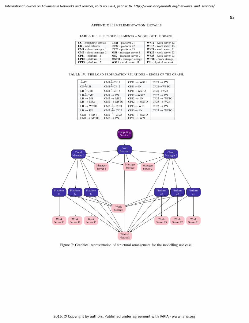
93



APPENDIX I: IMPLEMENTATION DETAILS

TABLE III: THE CLOUD ELEMENTS – NODES OF THE GRAPH.

CS - computing service CP21 - platform 21 WS12 - work server 12LB - load balancer CP22 - platform 22 WS13 - work server 13CM1 - cloud manager 1 CP23 - platform 23 WS21 - work server 21CM2 - cloud manager 2 MS1 - manager server 1 WS22 - work server 22CP11 - platform 11 MS2 - manager server 2 WS23 - work server 23CP12 - platform 12 MSTO - manager storage WSTO - work storageCP13 - platform 13 WS11 - work server 11 PN - physical network

TABLE IV: THE LOAD PROPAGATION RELATIONS – EDGES OF THE GRAPH.

5−→CS CM1 5−→CP11 CP11 → WS11 CP21 → PN

CS 5−→LB CM1 5−→CP12 CP11→PN CP21→WSTO

LB 5−→CM1 CM1 5−→CP13 CP11→WSTO CP22→W22

LB 5−→CM2 CM1 → PN CP12→WS12 CP22 → PNLB → MS1 CM2 → MS2 CP12 → PN CP22 → WSTOLB → MS2 CM2 → MSTO CP12 → WSTO CP23 → W23

LB → WSTO CM2 5−→ CP21 CP13→ W13 CP23 → PN

LB → PN CM2 5−→ CP22 CP13→ PN CP23 → WSTO

CM1 → MS1 CM2 5−→ CP23 CP13 → WSTOCM1 → MSTO CM2 → PN CP21 → W21

ComputingService

LoadBalancer Cloud

Manager 2Cloud

Manager 1

ManagerServer 1

Platform11

ManagerServer 2

PhisicalNetwork

Platform12

Platform13

Platform21

Platform22

Platform23

WorkServer 11

WorkServer 12

WorkServer 13

WorkServer 21

WorkServer 22

WorkServer 23

WorkStorage

ManagerStorage

Figure 7: Graphical representation of structural arrangement for the modelling use case.

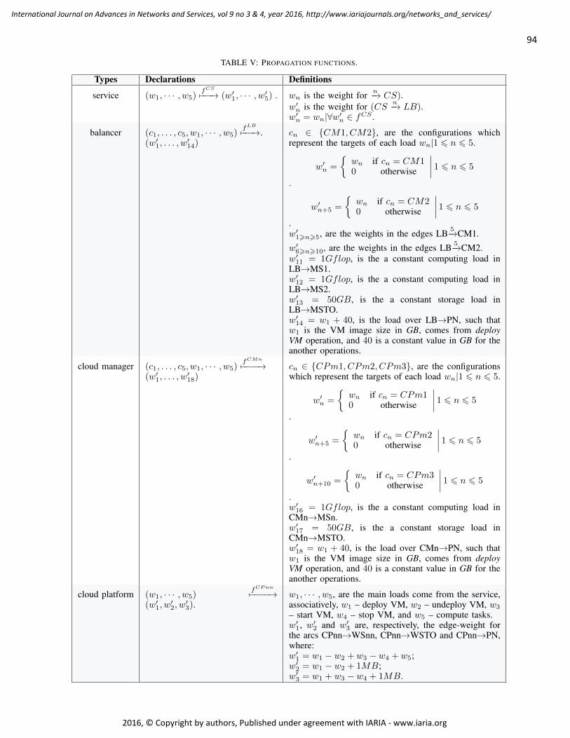
94



TABLE V: PROPAGATION FUNCTIONS.

Types Declarations Definitions

service (w1, · · · , w5)fCS

7−−−→ (w′1, · · · , w′5) . wn is the weight for n−→ CS).w′n is the weight for (CS

n−→ LB).w′n = wn|∀w′n ∈ fCS .

balancer (c1, . . . , c5, w1, · · · , w5)fLB

7−−−→.(w′1, . . . , w

′14)

cn ∈ {CM1, CM2}, are the configurations whichrepresent the targets of each load wn|1 6 n 6 5.

w′n =

{wn if cn = CM10 otherwise

∣∣∣∣ 1 6 n 6 5

.

w′n+5 =

{wn if cn = CM20 otherwise

∣∣∣∣ 1 6 n 6 5

.w′1>n>5, are the weights in the edges LB 5−→CM1.

w′6>n>10, are the weights in the edges LB 5−→CM2.w′11 = 1Gflop, is the a constant computing load inLB→MS1.w′12 = 1Gflop, is the a constant computing load inLB→MS2.w′13 = 50GB, is the a constant storage load inLB→MSTO.w′14 = w1 + 40, is the load over LB→PN, such thatw1 is the VM image size in GB, comes from deployVM operation, and 40 is a constant value in GB for theanother operations.

cloud manager (c1, . . . , c5, w1, · · · , w5)fCMn

7−−−−→(w′1, . . . , w

′18)

cn ∈ {CPm1, CPm2, CPm3}, are the configurationswhich represent the targets of each load wn|1 6 n 6 5.

w′n =

{wn if cn = CPm10 otherwise

∣∣∣∣ 1 6 n 6 5

.

w′n+5 =


∣∣∣∣ 1 6 n 6 5

.

w′n+10 =


∣∣∣∣ 1 6 n 6 5

.w′16 = 1Gflop, is the a constant computing load inCMn→MSn.w′17 = 50GB, is the a constant storage load inCMn→MSTO.w′18 = w1 + 40, is the load over CMn→PN, such thatw1 is the VM image size in GB, comes from deployVM operation, and 40 is a constant value in GB for theanother operations.

cloud platform (w1, · · · , w5)fCPnn

7−−−−→(w′1, w

′2, w

′3).

w1, · · · , w5, are the main loads come from the service,associatively, w1 – deploy VM, w2 – undeploy VM, w3

– start VM, w4 – stop VM, and w5 – compute tasks.w′1, w′2 and w′3 are, respectively, the edge-weight forthe arcs CPnn→WSnn, CPnn→WSTO and CPnn→PN,where:w′1 = w1 − w2 + w3 − w4 + w5;w′2 = w1 − w2 + 1MB;w′3 = w1 + w3 − w4 + 1MB.

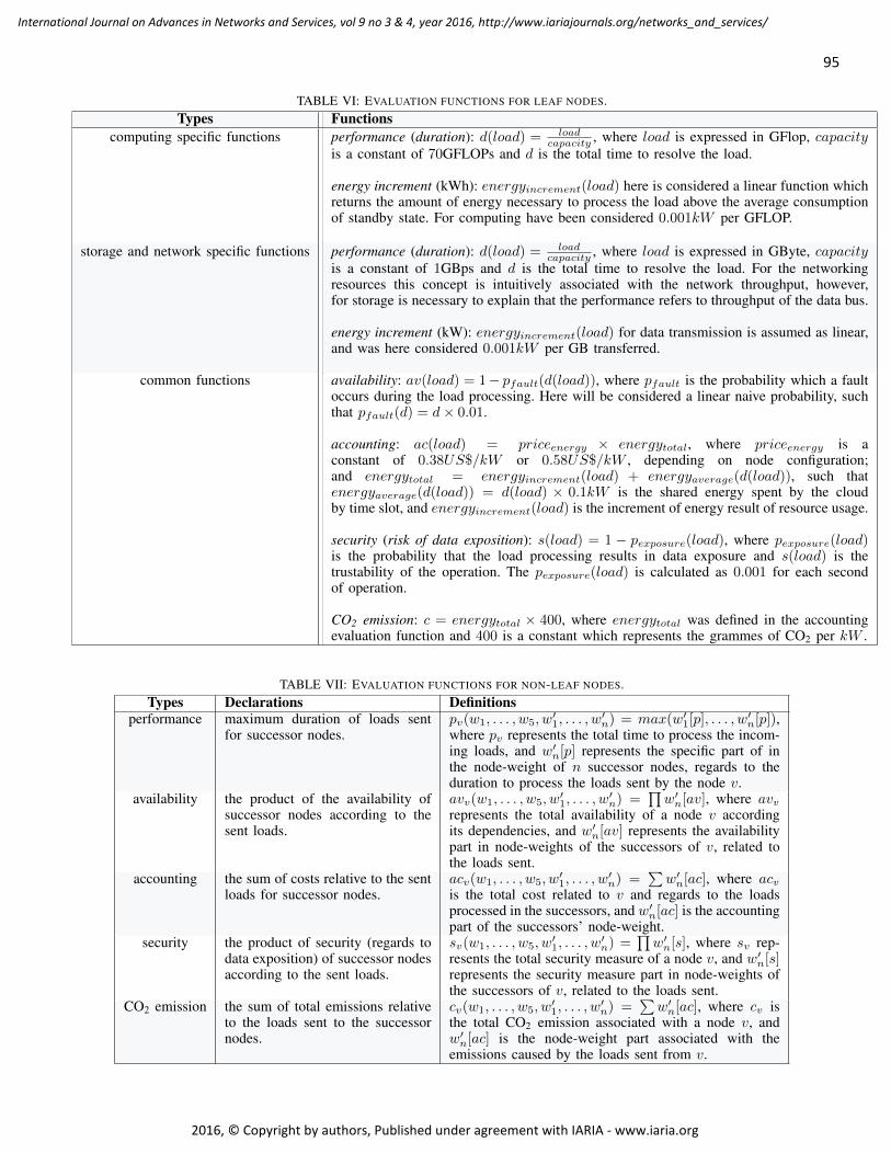
95



TABLE VI: EVALUATION FUNCTIONS FOR LEAF NODES.Types Functions

computing specific functions performance (duration): d(load) = loadcapacity , where load is expressed in GFlop, capacity

is a constant of 70GFLOPs and d is the total time to resolve the load.

energy increment (kWh): energyincrement(load) here is considered a linear function whichreturns the amount of energy necessary to process the load above the average consumptionof standby state. For computing have been considered 0.001kW per GFLOP.

storage and network specific functions performance (duration): d(load) = loadcapacity , where load is expressed in GByte, capacity

is a constant of 1GBps and d is the total time to resolve the load. For the networkingresources this concept is intuitively associated with the network throughput, however,for storage is necessary to explain that the performance refers to throughput of the data bus.

energy increment (kW): energyincrement(load) for data transmission is assumed as linear,and was here considered 0.001kW per GB transferred.

common functions availability: av(load) = 1− pfault(d(load)), where pfault is the probability which a faultoccurs during the load processing. Here will be considered a linear naive probability, suchthat pfault(d) = d× 0.01.

accounting: ac(load) = priceenergy × energytotal, where priceenergy is aconstant of 0.38US$/kW or 0.58US$/kW , depending on node configuration;and energytotal = energyincrement(load) + energyaverage(d(load)), such thatenergyaverage(d(load)) = d(load) × 0.1kW is the shared energy spent by the cloudby time slot, and energyincrement(load) is the increment of energy result of resource usage.

security (risk of data exposition): s(load) = 1 − pexposure(load), where pexposure(load)is the probability that the load processing results in data exposure and s(load) is thetrustability of the operation. The pexposure(load) is calculated as 0.001 for each secondof operation.

CO2 emission: c = energytotal × 400, where energytotal was defined in the accountingevaluation function and 400 is a constant which represents the grammes of CO2 per kW .

TABLE VII: EVALUATION FUNCTIONS FOR NON-LEAF NODES.Types Declarations Definitions

performance maximum duration of loads sentfor successor nodes.

pv(w1, . . . , w5, w′1, . . . , w

′n) = max(w′1[p], . . . , w′n[p]),

where pv represents the total time to process the incom-ing loads, and w′n[p] represents the specific part of inthe node-weight of n successor nodes, regards to theduration to process the loads sent by the node v.

availability the product of the availability ofsuccessor nodes according to thesent loads.

avv(w1, . . . , w5, w′1, . . . , w

′n) =

∏w′n[av], where avv

represents the total availability of a node v accordingits dependencies, and w′n[av] represents the availabilitypart in node-weights of the successors of v, related tothe loads sent.

accounting the sum of costs relative to the sentloads for successor nodes.

acv(w1, . . . , w5, w′1, . . . , w

′n) =

∑w′n[ac], where acv

is the total cost related to v and regards to the loadsprocessed in the successors, and w′n[ac] is the accountingpart of the successors’ node-weight.

security the product of security (regards todata exposition) of successor nodesaccording to the sent loads.

sv(w1, . . . , w5, w′1, . . . , w

′n) =

∏w′n[s], where sv rep-

resents the total security measure of a node v, and w′n[s]represents the security measure part in node-weights ofthe successors of v, related to the loads sent.

CO2 emission the sum of total emissions relativeto the loads sent to the successornodes.

cv(w1, . . . , w5, w′1, . . . , w

′n) =

∑w′n[ac], where cv is

the total CO2 emission associated with a node v, andw′n[ac] is the node-weight part associated with theemissions caused by the loads sent from v.

96



Multiradio, Multiboot Capable Sensing Systems for Home Area Networking Brendan O’Flynn, Marco De Donno, Wassim Magnin

Tyndall National Institute University College Cork

Cork, Ireland

email: [email protected]. [email protected], [email protected]

Abstract—The development of Wireless Sensor Networking technology to deploy in smart home environments for a variety of applications such as Home Area Networking has been the focus of commercial and academic interest for the last decade. Developers of such systems have not adopted a common standard for communications in such schemes. Many Wireless Sensor Network systems use proprietary systems so interoperability between different devices and systems can be at best difficult with various protocols (standards based and non-standards based) used (ZigBee, EnOcean, MODBUS, KNX, DALI, Powerline, etc.). This work describes the development of a novel low power consumption multiradio system incorporating 32-bit ARM-Cortex microcontroller and multiple radio interfaces - ZigBee/6LoWPAN/Bluetooth LE/868MHz platform. The multiradio sensing system lends itself to interoperability and standardization between the different technologies, which typically make up a heterogeneous network of sensors for both standards based and non-standards based systems. The configurability of the system enables energy savings, and increases the range between single points enabling the implementation of adaptive networking architectures of different configurations. The system described provides a future-proof wireless platform for Home Automation Networks with regards to the network heterogeneity in terms of hardware and protocols defined as being critical for use in the built environment. This system is the first to provide the capability to communicate in the 2.4GHz band as well as the 868MHz band as well as the feature of multiboot capability. A description of the system operation and potential for power savings through the use of such a system is provided. Using such a multiradio, multiboot capable, system can not only allow interoperability across multiple radio platforms in a Home Area Network, but can also increase battery lifetime by 20 – 25% in standard sensing applications.

Keywords - Smart Sensing; Low Power Consumption Protocols, Home Area Networks (HAN); Energy Management; Multiradio Systems.

I. INTRODUCTION Wireless Sensor Network (WSN) systems have the

potential to be ubiquitous in today’s Society in a myriad of applications such as Smart Homes, Building Energy Management (BEM), Home Area Networking (HAN), micro grid management, environmental monitoring and smart cities. New architectures, such as those described in the conference paper [1] and from which this paper evolved, are required to offer improved inter-operability, to improve

reliability of data communications and to address the spread spectrum requirements associated with next generation sensor systems through the development of smart radio systems. Currently available platforms exist that have multiple radios but these tend to operate in a single Industrial, Scientific and Medical (ISM) band (typically 2.4GHz) – and not in combination with the 868MHz ISM Band, which is ideal for the built environment due to its long range, low data rate properties.

This type of architecture has some interesting commercial applications for interoperable networks, Home Area Networks, commercial buildings and smart cities. Compared to single-end radio devices, it has the potential to provide increased connectivity in deployment, and can potentially reduce the interference impact on the network because the system can hop from ISM band to ISM band in an autonomous and opportunistic manner. The development of multiradio sensing architectures lends itself to interoperability between the different technologies that typically make up a heterogeneous network of sensors.

The value of WSNs as a sensing system is clear when you compare them to traditional wired sensing systems. Typically wired sensor systems are expensive to install with 70-90% of the cost of a sensor system installation relating to labor and wiring, which ranges from $40 to $2000 per linear foot of wiring [2]. As such, the wireless nature of WSN technologies makes them easier and cheaper to deploy than wired technologies.

However, a number of challenges still need to be addressed to ensure WSN technology achieves its’ full potential across all application areas. An abundance of communications technologies persist within the HAN domain, with no single technology identifying itself as the "one size fits all" solution.

The AUTonomic HomE area NeTwork InfrastruCture (AUTHENTIC) project [3][4] funded by the International Energy Research Centre (IERC) [5], sought to develop and deploy a HAN infrastructure capable of supporting opportunistic decision making pertaining to effective energy management within the home. This required the integration of key enabling heterogeneous technologies including a variety of physical sensors within the home (temperature, contact sensors, passive infra-red), cyber sensor sources (services) outside of the home (e.g., meteorological data, energy providers dynamic pricing sites) together with effective interfacing with the smart grid beyond the home. As part of the AUTHENTIC project (final demonstrators were

97



presented in 2015) the WSN group at Tyndall were developing the embedded systems and communications platforms to sense and transfer data in the built environment. The platform developed enables communications between the heterogeneous sensing systems that typically make up a HAN scenario in a power efficient implementation.

Section I of this paper introduces the subject matter and application space associated with wireless sensing solutions for the built environment. Section II reviews some of the state of the art in current wireless sensing system technologies, with emphasis on multiradio systems. Section III describes the “AUTHENTIC Board” developed within the project [1]. Section IV describes the multiradio functionality and Section V examines the results of initial range testing trials and tests carried out using the system to investigate power consumption characteristics of the platform. Section VI investigates the power savings enabled by this multiradio, multiboot platform, through the implementation of different communications protocols based on the system level tests carried out in Section V. Section VII concludes the work and outlines some directions for future research in this area.

II. PREVIOUS WORKS There are a variety of standards available (proprietary and

non-proprietary), which are widely used within the many deployments of HAN that exist. ZigBee, Bluetooth LE (Low Energy), IEEE 802.11x (Wi-Fi) are globally recognized as references in wireless communications and go far beyond the scope of WSN. Those technologies have been developed using the license-free ISM band of 2.4-2.5GHz, although ZigBee has an implementation for the 868MHz and the latest 802.11.n standard used by Wi-Fi offers support for both 2.4 and 5GHz. Indoor range above the GHz frequency is quite limited especially for indoor applications with dense obstacles. The Wi-Fi technology surpasses those issues with higher transmission power (up to 100 times higher than ZigBee/802.15.4), which is of course not suitable for battery powered systems in low power WSN deployments.

Although some manufacturers provide WSN systems using 868MHz or even 433MHz, it is more common to see them designed around proprietary technologies such as ZigBee. An interesting trade off investigated in this paper is the development of a system with the ability to adapt its communications channel to use the best radio link depending on the throughput and range requirements in any configuration.

Multiradio platforms are a subject of research for WSN as they offer some attractive characteristics and improvements over single radio WSN platforms. Multiradio systems with radios covering Wi-Fi, Bluetooth and 6LoWPAN (IPv6 over Low power Wireless Personal Area Networks) operating at the 2.45 GHz ISM band have reported to achieve enhanced robustness, latency and energy characteristics [ 6 ]. In a variety of implementations, multiradio systems operating at the 433MHz and 2.45 GHz ISM bands have been reported which use a preamble sampling technique in a wakeup radio implementation [7]. These multiradio platforms have been used to evaluate the performance of communications protocols in terms of power

consumption and latency over different duty cycle values and under various amounts of traffic loads. Kusy [8] reports on the development of a new dual radio network architecture to improve communication reliability in a wireless sensor network, but the approach was limited to a single channel implementation, where the 900MHz and 2.4GHz radios were used in parallel rather than in conjunction with power saving protocols. A multiradio platform for on the body WSN applications operating in 433MHz and 868Mz is reported in [ 9 ] with focus on the platform architecture. More consideration on the issues of antenna design for such devices is found in [10] [11]. A comprehensive survey of MAC protocols is given by Jurdak et Al in [12 ]. They survey, classify, and analyze 34 MAC layer protocols for wireless ad hoc networks, ranging from industry standards to research activites.

The BtNode V3 [13] platform features two radios. It incorporates a Chipcon CC1000 low power radio (433-915 MHz) and also has an additional ZV4002 Bluetooth radio (2.4 GHz) as shown in Figure 1.a. Similarly the Shimmer mote [14] and the Wasp Mote [15] feature a CC2420 IEEE 802.15.4 radio and can also be configured with an optional Bluetooth radio shown in Figure 1.b and Figure 1.c respectively. The Wasp Mote also has separate 868MHz and 900MHz radio modular plug-in boards however, in this instance only a single radio module can be operated at a time and true multiradio operation is not feasible. Similarly, the Tyndall Mote (Figure 1.d), has the capability for adding multiple radios. With the Tyndall mote, because of the planar implementation, several different radios could be stacked on top of each other and operate simultaneously.

The AUTHENTIC board described in this publication is not only a radio sensing platform but it can also be a repeater increasing the range of the network. Moreover, at the same time, the user can connect to each single platform in the network using a tablet or a smartphone via Bluetooth (for maintenance or data visualization).

The AUTHENTIC board has been designed with interoperability in mind, it can be used in existing deployments that use ZigBee or 868MHz protocols, to improving the network range without increasing the interference. From a protocol perspective, each board can work as an end node or base station/coordinator as well. In fact, if there are some changes in the network one node can reboot and operate as in base station mode using its multiboot functionality.

Similarly, the OPAL platform is an example of a multiradio platform where increased performance in terms of the network realization, latency, data throughput and power consumption were achieved compared to single radio platforms [16]. The OPAL platform is a high throughput sensing module that includes two onboard 802.15.4 radios operating in the 900MHz and 2.4GHz bands to provide communication diversity and an aggregate transfer rate of 3 Mbps. It embeds a 96 MHz Cortex SAM3U processor with dynamic core frequency scaling, a feature that can be used to fine-tune processing speed with the higher communication rates while minimizing energy consumption.

98



a.

b.

c.

d. Figure 1. Multiradio systems. a) Dual Radio BTnodeRev3 b) Dual Radio

Shimmer c) Wasp Mote ZigBee & Bluetooth Modules d) The Tyndall 25mm modular system

III. SYSTEM IMPLEMENTATION The aim of this system development is to provide a

future-proof wireless platform for HAN with regards to the network heterogeneity in terms of hardware and protocols currently in use and under development.

A specification process was undertaken with industry partners and service providers in the area of building management – to identify the core requirements associated with a wireless system for deployment in homes and offices.

The platform described in the following sections of this paper is a novel low power consumption multiradio system incorporating a 32-bit ARM-Cortex microcontroller and multiple radio interfaces - ZigBee/6LoWPAN/Bluetooth LE/868MHz platform, which features autonomous behavior to enable interoperability between systems utilizing different

radio front ends. It provides a solution for network congestion in environments such as HAN and Commercial Buildings in a credit card sized form factor shown in Figure 2. It also provides better interoperability than the usual wireless sensor devices approach, enhancing the communicability between different network entities (sensor nodes, smart meters, media, smartphones), and driving the wireless sensor networks to the smart cities application space.

Figure 2. AUTHENTIC Credit Card Form Factor Platform.

The four main issues that need to be considered prior to selecting any unit or design approaches are: over all power consumption, cost, complete module size and user friendliness. Technical features assessed and considered included: functionality requirements as regards actuation and control, quality of service, latency, number and types of sensors/meters and interfaces, programming methods (wireless/non wireless), power supplies/energy harvesting compatibility, radio frequency band, standards/non standards communications and data transmission range.

Figure 3. Block diagram of AUTHENTIC Platform functionality.

99



In conjunction with these end users, as part of our system specification, three communication standards were identified as being needed within the HAN environment: ZigBee – 2.4GHz, 6LoWPan – 2.4GHz, Bluetooth Low Energy – 2.4GHz, as well as a non-standards based ISM band 868MHz transceiver as a response to the 2.4GHz limitations identified - bandwidth congestion and data loss associated with non line of sight (NLOS) effects of the building structure limited RF range. The board has been designed around the standard ARM CORTEX-M3 based microcontroller, which offers a good trade-off between power consumption and performance. See Figure 3 for an overview of features and functionalities.

The final embedded system was designed around a credit card form factor (shown in Figure 4) and deployed in offices and homes for preliminary tests and characterization

Microcontroller: The heart of the system is the ATMEL SAM3S8C microcontroller, a 32-bit ARM Cortex M3 Core. 64MHz Maximum, 512KB flash, 64KB RAM, USB 2.0.

External Flash Memories: Two external flash memories: 128MB NAND flash for data logging, 16MB NOR-flash for code execution. The two memories are connected to the microcontroller External Bus Interface (EBI).

Radio Communication: The platform integrates three radio chips: Bluetooth Low Energy radio chip, (manufacturer: NORDIC, model: NRF8001), ZigBee/6LoWPAN radio chip, (manufacturer: ATMEL, model: AT86RF231), Sub-GHz radio chip (868MHz), (manufacturer: ST Microelectronics, model: SPIRIT1).

Sensors: Two sensors were interfaced via an I2C interface: temperature sensor, accuracy: ±0.5°C, (manufacturer: MAXIM, model: MAX31725MTA+), light sensor, range: 0.045 Lux to 188,000 Lux, (manufacturer: MAXIM, model: MAX44009EDT+T). These are used for detecting in-home activity monitoring occupancy through lighting usage.

Battery: The battery used is a lithium prismatic battery with a capacity of 1300mAh, which is recharged through the USB port or through the use of energy harvesting systems compatible with the built environment [17].

Figure 4. AUTHENTIC multiradio embedded system.

IV. MULTIRADIO FUNCTIONALITY In this section the functionality of the AUTHENTIC

platform is presented in terms of its communication architectures, the multiradio and multiboot capabilities embedded in the system.

A. Communication Architectures using Multiradio Systems In the context of “crowded radio frequency spectrum”, a

wireless sensor network composed with a number of the proposed devices’ architectures can automatically adapt to the most reliable frequency communication channel based on the local interferences. This type of architecture has some interesting commercial applications for interoperable networks, HAN’s, commercial buildings and smart cities. Compared to single-end radio devices, it has the potential to provide increased connectivity in deployment, and can potentially reduce the interference impact on the network as the system can hop from ISM band to ISM band in an autonomous and opportunistic manner.

Figure 5. AUTHENTIC multiradio system in operation

By developing smart mechanisms for multi-protocol routing between the different radios, this architecture can potentially reduce the number of repeaters (and thus the infrastructure cost) compared to a standard single ended radio platform. In addition, multiradio systems provide better interoperability with Off-The-Shelf wireless devices, many of which operate on a variety of different standards and which may constitute a typical smart home deployment.

100



From a research point of view, such a platform can be used to develop and evaluate firmware/wireless protocols using different frequency bands.

The multiradio concept is illustrated in Figure 5 which shows how, by jumping between the 2.4GHz and 868MHz frequency bands, a connection can be made between remote clusters of ZigBee nodes, which are in different locations or separated by a congested spectrum making communication at 2.4GHz difficult.

Thus the network automatically switches to the 868MHz frequency in order to maintain communication with the out of range node. In that case, one node from the first cluster will act as a virtual “dual sensing” node, providing two inputs to the ZigBee Network.

B. Multiradio Aspect The Bluetooth and 868MHz multiradio functionality has

been tested as a proof of concept in a HAN as part of the AUTHENTIC deployment in office environments and in homes (for open field testing, the system was deployed temporarily outside).

To evaluate the capabilities of the multiradio functionality, the remote node sends data (light, temperature or other peripheral sensor) to the base station using the 868MHz radio or the 2.4GHz ZigBee network. The base station then sends the received data to a Smart Phone/HAN gateway using the Bluetooth interface that displays the data stream (in this case, temperature and light level from the remote sensor) as shown in Figure 6.

Figure 6. AUTHENTIC multiradio system

C. Multiboot - Autonomous System Implementation Multiboot capability enables the system to boot up and

run according to various boot images [18] [19], which are stored in various sectors (region) of memory – see Figure 7.

Figure 7. AUTHENTIC Multiboot reconfigurability

To facilitate energy savings at an embedded system level, the multiboot configuration of the system will allow the platform to host two different applications and jump between them (via a boot loader). The applications can and will use different radios in future deployments, which will be useful for overcoming transmission issues in a congested/noisy environment. The targeted example is the mote running a ZigBee 2.4GHz application and an 868MHz application. Failing to transmit data at 2.4GHz due to electromagnetic effects or long range requirements, the node would switch to the 868MHz application to operate in a less congested ISM band. This behavior would be coordinated among the network nodes in protocols under development. In this case, the idea is to allocate memory regions to specific applications.

The Multi-Application Software Management tool acts as a main application that we will call “Leader”. The Leader is programmed in a specific area of the memory and will act as what is commonly known as a Bootstrap Loader. The particular boot state functionality can be associated with a range of communications modalities say ZigBee, Bluetooth or Wireless Modbus according to application requirements associated with energy consumption, latency or Quality of Service.

The Leader can access any location of the memory. The applications that will contain the required functionalities of the system (e.g., sensing, communication) will be described as “Users”. The Leader can then grant the leadership to the different Users that will need to return the leadership to the Leader (different solutions are possible for the latter).

101



The Leader will provide an API (Application Programming Interface) in order to modify intrinsic parameters of the system (e.g., system clock frequency, timers etc.). Thus, this functionality will considerably reduce the complexity of the development from the user developer’s point of view.

From a smart home/building management system deployment perspective, it will provide an essential software management tool for multiradio platforms.

V. RESULTS

A. AUTHENTIC Board Power Characterization To carry out the energy consumption tests, the following

modalities were implemented as shown in Table I.

TABLE I. SYSTEM POWER CONSUMPTION IN DIFFERENT MODES

Symbol Operational Mode Measured Value Unit

ITX868

Current consumption in TX mode 868MHz module, POUT = +12 dBm, all components on

43.98 mA

Isb868 Current consumption in standby mode 868MHz module, all components on

28.24 mA

ITXBLE 0dBm

Current consumption in TX mode BLE module, POUT = 0 dBm, all components on

24.80 mA

IsbBLE Current consumption in standby mode (between 2 transmissions) BLE module, all components on

17.29 mA

ITX, ZigBee

1

Current consumption in TX mode ZigBee module, POUT = +3 dBm, all components on, 1 led on

64.07 mA

ITX, ZigBee

2

Current consumption in TX mode ZigBee module, POUT = +3 dBm, all components on, 1 led off

71.12 mA

Isleep1 Current consumption in sleep mode (microcontroller) and all the other components on

15.73 mA

Isleep2 Current consumption in sleep mode (microcontroller) and all the other components off

3.18 mA

Isleep3

Current consumption in deepest sleep mode (microcontroller) and all the other components on

3.1 mA

Isleep4 Current consumption in deepest sleep mode and components off / removed

3.5 µA

The MCU is programmed to turn on all the devices, setting the output power of the module to (+12 dBm for 868 MHz module, 0 dBm for BLE, +3 dBm for ZigBee), start the transmission of a single packet (1 byte length) and then put it in standby mode. Sleep mode tests include the MCU turning

on all the devices before going into sleep mode, turning off all the devices and entering sleep mode, turning on all the devices and entering deepest sleep mode and turning off all the devices and going into deepest sleep mode.

For the 868 MHz tests, GFSK (Gaussian frequency-shift keying) modulation with the Gaussian filter “BT Product” set to 1 was used. For the Bluetooth LE modules the default Gaussian filter used is 0.5. For the ZigBee module quadrature phase-shift keying (QPSK) modulation was used. Table I shows the results of all tests in different modes. These provide the building blocks for developing low-power networking algorithims for optimising the lifetime of the WSN systems and QoS parameters.

B. Multiradio Range Test Comparison 1) Indoor Non Line of Sight (NLOS) range testing

This section focuses on the NLOS testing of the 868 MHz, Bluetooth and ZigBee radio modules on the AUTHENTIC Board. Two boards are used: one acts as a sensing node and one as a Base Station.

The node reads data from the temperature sensor as well as received signal strength indication (RSSI) values. This is then sent to the Base Station where it is converted into a value expressed in °C (minimizing energy consumption associated with processing on the node), which is in turn sent to our visual interface (a smartphone connected via Bluetooth).

The test took place in an office environment consisting of open plan cubicles, closed offices, coffee dock facilities and meeting rooms in a simulated “home environment”. The node (represented by the star) was kept stationary while the base station and the smartphone moved around the entire area for data gathering at the different frequencies under test. In Figures 8, 9, 10, the areas where the data is received perfectly are reported in green, in orange the areas where the signal is poor and the data is received intermittently, in red the areas where there is no signal and data is not received.

Theory would suggest that the range associated with lower frequency (868MHz) ISM bands would significantly outperform higher frequency ISM bands (2.4GHz). In this experiment, the difference is little more than a 10% improvement (see Table II).

TABLE II. COMPARISON OF RANGE FOR INDOOR NLOS TESTS

Radio Appoximate Area Covered

Max. distance (Line of sight)

868 MHz 130.4 m2 11.4 m Bluetooth LE 60.04 m2 7 m ZigBee 108.6 m2 10.6 m

We expected 868MHz to be much better than ZigBee, a

possible reason (under investigation) is that the 868MHz data rate (500 kbps) is higher than the ZigBee one (250 kbps) and there is a tradeoff between the range and the data rate. Moreover, the modulation used by the modules are different: the value of Eb/N0 (noise power per unit bandwidth) of the offset-QPSK is less than that of the GFSK; this means that the bit error rate is better for the ZigBee module operating at

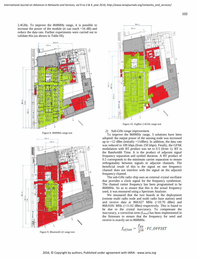
102



2.4GHz. To improve the 868MHz range, it is possible to increase the power of the module (it can reach +16 dB) and reduce the data rate. Further experiments were carried out to validate this (as shown in Table III).

Figure 8. 868MHz range test

Figure 9. Bluetooth LE range test

Figure 10. ZigBee 2.4GHz range test

2) Sub-GHz range improvement. To improve the 868MHz range, 3 solutions have been

adopted: the output power of the sensing node was increased up to +12 dBm (initially +11dBm). In addition, the data rate was reduced to 100 kbps (from 250 kbps). Finally, the GFSK modulation with BT product was set to 0.5 (from 1). BT is the Bandwidth Time. It is the product of adjacent signal frequency separation and symbol duration. A BT product of 0.5 corresponds to the minimum carrier separation to ensure orthogonality between signals in adjacent channels. The beneficial result of this is the signal on one frequency channel does not interfere with the signal on the adjacent frequency channel.

The sub-GHz radio chip uses an external crystal oscillator that provides a clock signal for the frequency synthesizer. The channel center frequency has been programmed to be 868MHz. So as to ensure that this is the actual frequency used, it was measured using a Spectrum Analyser.

We measured that the two boards in the deployment (remote multi radio node and multi radio base station) send and receive data at 868.027 MHz (+10.70 dBm) and 868.0181 MHz (+11.02 dBm) respectively. This is found to be due to the crystal inaccuracy. To compensate the inaccuracy, a correction term (foffset) has been implemented in the firmware to ensure that the frequency for send and receive is exactly set to 868MHz.

103



Where fXO is the frequency of the crystal oscillator (52MHz) and FC_OFFSET is a 12-bit integer set by the FC_OFFSET registers of the radio chip.

Figure 11. Output power.

After this compensation, the 2 boards had the center frequency at 868.00MHz (Figure 11) and another range test has been made in the same environment of the previous tests with 2 AUTHENTIC boards (one as node remote and one as base station) and the result has been reported in Figure 12 and Table III below showing the maximum range obtained using the 868MHz radio.

Figure 12. 868MHz range test after compensation

As can be seen from a comparison with the initial set of results reported in [1] and shown here in Table II, we achieved an improvement of 60% in performance (area covered) with the new configuration settings for the AUTHENTIC boards operating in the 868 MHz band.

TABLE III. RANGE TESTING 868 MHZ BAND USING OPTIMISED CONFIGURATION SETTINGS

Radio Approximate Area Covered 868MHz (Test 1) 130,4 m2 868MHz (Test 2) 211,5 m2

3) Outdoor Line of Sight (LOS) range testing

An open field is one of the simplest and most commonly used environments for RF range tests. In this section, tests for the three modules on the AUTHENTIC Board (868MHz, Bluetooth, and ZigBee) are reported. The tests took place in a sports field in University College Cork, which offered a long range LOS measurement.

868MHz: To test the Sub-GHz module, two AUTHENTIC boards were used, one as Node Remote and one as Base Station. The first reads data every four seconds from the temperature sensor and sends it to the Base Station. The maximum range measured was 193m.

Bluetooth: For this test, two devices were used: one AUTHENTIC Board and a smartphone. The board was left stationary and the smartphone was moved around the area checking if the connection was still available or not. The maximum LOS distance measured was 18.4m.

ZigBee: To test the ZigBee module, two AUTHENTIC boards (one as Trust Center and one as Occupancy Sensor) were used along with a RF231USB-RD USB Stick (as Remote Control). The Trust Center creates the network and the other two devices join it. After this, the Occupancy Sensor reads the value of the LED (on/off) and sends it every four seconds to the Remote Control that moves around the area. The maximum range measured was 193m.

The maximum distance measured in Line of Sight for both the ZigBee and 868MHz system was 193m, but this value could be greater and additional tests need to be carried out to establish the maximum range for each. The maximum range achieved was due to the presence of physical obstacles (walls/buildings, which would have interfered with the LOS measurements at the maximum extremity of the test location. The results are tabulated in Table IV.

TABLE IV. COMPARISON OF RANGE FOR OUTDOOR LOS TESTS

Radio Max. distance (Line of Sight)

868MHz 193m * Bluetooth LE 18.4m ZigBee 193m *

* Limit of the field measurement, not the technology

VI. AUTHENTIC MULTI HOP PROTOCOL IMPLEMENTATION

The AUTHENTIC network has been designed to be an auto configurable network, this means that the network is autonomous in operation and has the capability to reconfigure itself. It is composed of one base station (that acts as both a router and gateway) and sensor nodes (sensing nodes that read data from the sensors on board and send the sensor data values to the base station/gateway) as shown in Figure 13.

104



Figure 13. The AUTHENTIC network topology

At system start up, the base station creates a sub-1GHz network with the sensor nodes by transmitting a broadcast message to the nodes and waiting for their reply.

When the node receives the broadcast packet, it saves the base station’s address in its memory and replies with an ACK to confirm that it has received the message.

When the base station receives the ACK, it checks the Received Signal Strength Indication (RSSI) to be sure that the link with the node is a robust one. If the RSSI value is higher than the threshold (it is taken to be -75 dBm), then the base station saves the node’s address in its list of the sub-1GHz addresses, so as to be able to build an appropriate routing table. If the RSSI value is lower than the threshold, the base station sends another message to the node in order to change the radio communication to ZigBee. The default start up mode is in the 868MHz band operation mode. Two possible factors can affect the RSSI value: interference and the distance between the node and the base station. In these cases it is better to switch to another frequency.

Figure 14. Node's state machine

The node goes into RX mode every time it sends a packet to the base station in order to receive the command to switch to ZigBee. The protocol state machine for the node is shown in Figure 14. The node, after sending the ACK message regarding the broadcast packet, goes into RX mode for a certain period (it is taken for the purposes of these experiments to be 1 second). During this period the only message that it can receive is the command to change its communication to ZigBee due to the RSSI level measurements taken. If so, it will reboot (using the multi boot functionality described in [1]) with the ZigBee application and waits for the creation of the ZigBee network.

If the node doesn’t receive any command from the base station it assumes that it is part of the sub-1GHz (868MHz) network, and goes into sleep mode (to reduce power consumption) for a random period between 4 and 5 minutes (Tsleep). The node then wakes up, reads the data from the sensors on board (temperature and light level) and sends them to the base station. Once the data packet is sent, the node again enters in RX mode for 2 seconds so as to receive an appropriate command from the base station, after that it goes into sleep mode for Tsleep, then it wakes up, sends the sensors readings and so on.

Tsleep is a randomly assigned value to avoid the case that all the nodes send their sensor readings at the same time. This will reduce the probability of packet collision between the transmissions with the resultant requirement for retransmissions and increase in associated energy consumption.

The base station, after the broadcast message, communicates with each node that has replied to the broadcast, and saves all their addresses in 2 lists, one for the sub GHz network (that contains the nodes’ addresses with RSSI higher than the threshold) and one for the ZigBee network (that contains the nodes’ addresses with RSSI lower than the threshold). Based on these tables, the coordinator is in a position to develop an appropriate network structure. The sub GHz network is created first, after which the base station starts the creation of the ZigBee network. Once the two networks have been defined, the basestation enters sleep mode to save power. The system can be woken up by receiving sensor data messages from the nodes associated with the 2 networks created. This wake up is instigated by an interrupt based on a received data packet used to wake the microcontroller up out of standby mode.

For each message received, the base station sends the sensor data to a GUI enabled device connected via the Bluetooth interface on the AUTHENTIC Board (to any standard smartphone, tablet, PC etc.). The GUI displays data in real time from the different nodes and stores these in an associated database for analysis. The base station checks if the RSSI value of that node is higher or lower than the threshold (in this case -75 dBm). Only if it is lower than -75 dBm will the base station send a message to the node in order to switch to ZigBee network. When the node receives this command it sends an ACK to the base station to confirm that the message has been received and it reboots with the ZigBee application mode operational.

105



When the base station receives the ACK, it removes the node’s address from the sub GHz addresses list and adds it to the ZigBee addresses list. The packet structure is shown in Figure 15.

Prea mble Sync Length Dest.

Address Source Address

Con trol

Seq. No. ACK Pay

load CRC

Figure 15. The AUTHENTIC Board Zigbee packet structure

Where: Preamble is a signal to synchronize transmission timing

and it is a programmable field from 1 to 32 bytes; Sync is the synchronization word; Length is the packet length; Dest. Address is the destination address and can be set

to a single, broadcast or multicast address; Source Address is the address of the transmitting board; Control is the control field of the packet; Seq. No. contains the sequence number of the

transmitted packet. It is incremented automatically every time a new packet is transmitted;

ACK is the acknowledgement field. If set to 1 means that it is the acknowledgement packet;

Payload is information data; CRC is the error detecting code to detect errors in the

data. The base station sends periodically (every 15 minutes)

the general broadcast message in order to contact new nodes that did not reply at the first message or to contact any of the nodes that need to reboot so they can join the network. Nodes that are already in the network will ignore the message.

The use of this protocol shows the interoperability between the different wireless technologies (Bluetooth, ZigBee, and 868MHz). It is proposed that this system is a solution for network congestion because it reduces interference in one particular frequency band. If interference is encountered in one band then the system simply changes the operational ISM band to avoid it.

It is also a good solution to reduce power consumption associated with an individual nodes’ operation. In the first instance, power savings are enabled due to the fact that the nodes and the base station are in low-power sleep mode if they don’t need to transmit data. Moreover, since the base station is monitoring the RSSI signal levels, redundant and energy wasteful transmissions are eliminated (in the case that the node continues to transmit data but the base station can’t receive them - because it is out of range or there is too much interference in the network).

An evaluation of potential power savings associated with the new protocol has been carried out regarding a network composed of one Base Station and three nodes and based on the power consumption reported in Table I, assuming to power the boards with a 3V battery, to transmit data every 5 minutes and then go in sleep mode.

In a scenario where three nodes join the sub-1GHz network and when the RSSI level referring to one node is lower than the threshold it joins the ZigBee network, the

estimated power consumption of the Base Station is 52.13mW and 14.43mW for a single node.

As previously outlined, the Base Station is in standby mode when it is not transmitting or receiving and the nodes go into sleep mode after sending the data read from the temperature and light sensors.

In a single radio scenario, where only the ZigBee network is available, it can happen that the nodes send the sensors data to the Base Station but it cannot receive them because of the interferences or long range issues, so the nodes transmit uselessly wasting power. In this case the estimated power consumption of the Base Station is 55.87mW and 16.83mW for a single node.

System energy consumption for the multiradio platform was calculated based on a model which was developed using empirically derived power measurements. These measurements are reported in Table I, and are based on the board being powered by a 3V battery. The operational duty cycle for the sensor nodes was selected to be 5%. The system is considered to be in sleep mode for the rest of the cycle.

From this energy model, we can see that the power consumption of the node that uses an appropriate communication protocol associated with a multiradio system (14.43mW) is reduced by approximately 15% compared to a node that works in a single radio system (16.83mW). This will translate to an increase in battery lifetime of 10-15% in a typical application (based on a standard AA battery).

VII. CONCLUSIONS & FUTURE WORK Interoperability between communications protocols

operating using different radio technologies is a major issue within the realm of wireless sensor technology where numerous wireless sensor technologies could be operating in the same vicinity. Middleware is one software solution that aims to overcome this problem. Middleware runs at either the gateway or cloud level and incorporates drivers for numerous protocols (ZigBee, Z-Wave and EnOcean for example).

This paper has shown how multi radio architectures and networks offer the possibility of increased interoperability and energy savings at a network and node level and thus are ideal for use in such HAN architectures. In addition, the multiradio architectures described address some of the issues associated with the fact that in the resource-constrained systems typically used in sensing systems for the built environment, energy is often the primary constraint and impacts on all aspects of the sensor system.

This work describes the development and preliminary characterization of a novel low power consumption multiradio system incorporating multiple radio interfaces - ZigBee/6LoWPAN/Bluetooth LE/868MHz platform. It provides a solution for network congestion in environment such as Home Area Network and Commercial Buildings in a credit card sized form factor. The multiradio sensing system shows the potential for such systems to improve interoperability between the different wireless technologies enhancing the communications between heterogeneous network entities (Sensor Nodes, Smart Meters, Media, Smart Phones), and driving the Wireless Sensor Networks use case in the built environment. The configurability of the system

106



can increase the range between single sensor points and can enable the implementation of adaptive networking architectures of different configurations.

Additional characterization and optimization of the system in a variety of environments is underway and development of frequency hopping protocols to maximize the potential of the multiradio system and its possibilities to maximize system lifetime of a WSN in a Smart Home or office environment through the development of networking protocols leveraging off the platforms capabilities.

ACKNOWLEDGMENT The authors would like to acknowledge the support of

Enterprise Ireland and the International Energy Research Centre (IERC) for funding the AUTHENTIC project (TC20121002A/B). This publication has emanated from research supported in part by Science Foundation Ireland (SFI) and is co-funded under the European Regional Development Fund, Grant Number 13/RC/2077-CONNECT. Aspects of this work have been funded by the European Union Horizon 2020 project MOEEBIUS under grant agreement 680517.

REFERENCES [1] B. O’Flynn, M. De Donno, and W. Magnin, “Multiradio

Sensing Systems for Home Area Networking and Building Management,” The Fifth International Conference on Smart Cities, Systems, Devices and Technologies (SMART 2016), IARIA, May 2016, pp. 25-30, ISSN: 2308-3727, ISBN: 978-1-61208-4763.

[2] F. Zhao and L. Guibas, Wireless Sensor Networks: An Information Processing Approach, ISBN-9781558609143, Elsevier, Chapter 8, pp. 294, 2004.

[3] AUTHENTIC Webpage, http://www.creativedesign.ie/ierc_test/?homeareanetworks=AUTHENTIC-for-home-area-networks-han 2016.11.25

[4] K.Curran, Recent Advances in Ambient Intelligence and Context-Aware Computing, IGI global book series Advances in Computational Intelligence and Robotics (ACIR)(ISSN: 2327-0411), Chapter 10, pp. 155-169.

[5] IERC Website, http://www.ierc.ie/ 2016.11.25 [6] M. T. Delgado, H. Khaleel, C. Pastrone, and M. A. Spirito,

“Underlying connectivity mechanisms for multi-radio wireless sensor and actuator networks,” The 9th International Conference on Wireless and Mobile Computing, Networking and Communications (WiMob 2013), IEEE, Oct 2013, pp. 408-413.

[7] J. Ansari, X. Zhang, and P. Mahonen, “Multi-radio medium access control protocol for wireless sensor networks,” Int. J. Sen. Networks, 8(1):47-61, 2010.

[8] B. Kusy et al., “Radio diversity for reliable communication in wsns,” in Proc. Int. Symp. Inform. Process. Sensor Networks.,Chicago, IL, 2011, pp. 270–281.

[9] J. Buckley et al.,“A novel and miniaturized 433/868mhz multi-band wireless sensor platform for body sensor network applications,” Ninth International Conference on Wearable and Implantable Body Sensor Networks (BSN 2012), May 2012,, pp. 63-66, ISBN: 978-0-7695-4698-8.

[10] L. Loizou, J. Buckley, and B. O’Flynn,” Design and analysis of a dual-band inverted-f antenna with orthogonal frequency-controlled radiation planes,” Antennas and Propagation, IEEE Transactions on, 61(8):3946-3951, 2013.

[11] L. Loizou, J. Buckley, B. O’Flynn, J. Barton, C. O’Mathuna, and E. Popovici,” Design and measurement of a planar dual-band antenna for the Tyndall multiradio wireless sensing platform,” In Sensors Applications Symposium (SAS 2013) IEEE, Feb 2013 pp. 11-14, ISBN: 978-1-4673-4636-8.

[12] R. Jurdak, C. V. Lopes, and P. Baldi, “A survey classification and comparative analysis of medium access control protocols for ad hoc networks.” IEEE Commun. Survey. Tutorials, vol. 6, pp. 2–16, Jan. 2004.

[13] BTNode http://www.btnode.ethz.ch/ 2016.11.25 [14] Shimmer Mote link www.shimmer.com 2016.11.25 [15] http://www.libelium.com/products/waspmote/hardware

2016.11.25 [16] R. Jurdak, K. Klues, B. Kusy, C. Richter, K. Langendoen, and

M. Brunig, “Opal. A multiradio platform for high throughput wireless sensor networks,” Embedded Systems Letters, IEEE, 3(4):121-124, 2011.

[17] C. O’Mathuna, T. O'Donnell, R. Martinez-Catala, J. Rohan, and B. O'Flynn, “Energy Scavenging For Long-Term Deployable Wireless Sensor Networks,” Talanta, 75 (3):613-623.

[18] D. Fuji, T. Yamakami, and K. Ishiguro, “A fast-boot method for embedded mobile Linux: Toward a single-digit user sensed boot time for full-featured commercial phones,” Proc. - 25th IEEE Int. Conf. Adv. Inf. Netw. Appl. Work., (WAINA 2011), March 2011, pp. 81–85, ISBN 978-0-7695-4338-3.

[19] C. W. Chang, C. Y. Yang, Y. H. Chang, and T. W. Kuo, “Booting time minimization for real-time embedded systems with non-volatile memory,” IEEE Trans. Comput., vol. 63, no. 4, pp. 847–859, 2014.

107



Analyzing the Performance of Software Defined Networks vs Real Networks

Jose M. Jimenez, Oscar Romero, Albert Rego, Jaime Lloret Universidad Politécnica de Valencia

Camino Vera s/n 46022, Valencia (Spain) email: [email protected], [email protected], [email protected], [email protected]

Abstract—Emulators and simulators provide an easy way to reduce hardware needs in experiments. Because of that, network researchers use applications that allow them to emulate or simulate networks, like Mininet in Software Defined Networks. It is desired to obtain very close results between the ones given in a virtual network and the ones obtained when the real network hardware is implemented in order to avoid using too much hardware in complex experiments without gathering unreal results. In this paper, we compare the experimental results obtained when a virtual network is generated by using Mininet versus a real implemented network. We have compared them varying the Maximum Transmission Unit (MTU) on Internet Protocol version 4 (IPv4) packets. Ethernet, Fiber Distributed Data Interface (FDDI), and Wireless Local Area Network 802.11 (WLAN 802.11) MTUs have been used in our experimental tests. We have worked with different link capabilities and generated traffic with different bandwidth.

Keywords- SDN; OpenFlow; Mininet; MTU; virtualization; bandwidth; jitter.

I. INTRODUCTION In the field of computer networks, the researches usually

use programs that allow us to emulate or simulate networks. This is because, in most cases, we do not have the necessary devices needed to create complex networks, but we need to know if these programs are reliable [1]. There are emulators and simulators as Omnet++ [2], OPNET [3], NS-2 [4], NS-3 [5] Netsim [6], GNS3 [7], etc. that are frequently used to create computer networks.

Deployment of network is very quick in virtual environment, even if it is needed a large number of resources, which is always practically almost impossible to implement with real hardware. Problem solving or troubleshooting capability is still easier than real implementations. Note that a network researcher has to keep in mind that the results obtained from a virtual network should be similar from those obtained by the real hardware network. If there is a significant difference between results of virtual network and real network, then the research work should not be taken into consideration. As a network test bed gives almost the same results as the real implemented network, then it saves a large amount of time, complexity and a lot of resources.

In general, network devices perform the transport and the control function. But, configuring a great amount of devices and changing the configuration efficiently to work properly, it means a big challenge for networking professionals.

Today's, computer network world is able to offer a large amount of functionalities suited to the requirements of users. A new technology, named Software Defined Networking (SDN) [8] appears to increase the efficiency and reduce the cost of network configuration.

Figure 1 shows the components of SDN in a layered structure. The first layer consists of some frequently used tools of monitoring and depuration. The tool “Oftrace” is used for analyzing and parsing Openflow message from network dump. “Oftrace” provides a library which analyzes and parses the message from TCP dump or Wireshark [9]. Loops or cyclic path can cause critical problems in SDN. “Oflops” is a tool to catch the loop mechanism in the software defined networks. It mentions the data packets in the loop which are not able to leave the network [10]. “Openseer” is a CGI script which helps to plot that data effectively in SDN [11]. In Controllers Layer there are few controllers which are used in SDN. More often, controllers are called the Brain of Network which controls and manages the software defined network. Floodlight, Open Daylight, Beacon, Nox are among the frequently used controllers in SDN [12]. Flow Visor ensures that multiple isolated logical networks can share the same topology and hardware resources of a network. It places as a transparent proxy between OpenFlow switches and OpenFlow controllers. The isolated logical network is named slice of the network and flow visor is named slicing software in SDN [13]. In SDN environment, OpenFlow switches are used to forward the packets. OpenFlow switches are either a software program or a hardware device which is compatible with OpenFlow protocols. Some of the commercial switches are available in market like HP, Nec, Juniper, etc. [14]. Mininet is used to create realistic virtual network within seconds on a single machine that could be able to run real kernel, switch and application code [15].

There are few emulators and simulators which are frequently used to run and control the technology SDN from a single screen. Some of them are NS-3, Estinet 9.0 [16], OmNet ++, Mininet, etc.

108



Figure 1.Key component of SDN in layered structure.

In this paper, we show the comparison among the obtained results from the virtual networks and from the real implemented networks. With the assessment of these results we are able to find the significant differences, which may be very useful for the researchers who all are performing their research work in Networking Industry. We have performed different experiments over Mininet and real implementation to have a good understanding of the network behavior in both scenarios. To do a detailed study, we must send data packets of different properties and compare the results. We used the data packets with different Maximum Transmission Unit (MTU) on IPv4. These sizes of packets are usual for Ethernet version 2, Ethernet with Logical Link Control (LLC), Point-to-Point Protocol over Ethernet (PPPoE), WLAN, Token Ring and FDDI.

This paper is an extended version of a conference paper published in [1].

The rest of the paper is structured as follows. In Section II, we discuss existing related works. In Section III, we introduced all resources that we used in our test bench. Measurement results and our discussion and analysis are shown in Section IV. Section V shows the conclusion and future works.

II. RELATED WORKS In the past, a few researchers have accomplished their

work in the area of SDN and investigated the performance of multimedia delivery over SDN. Furthermore, in the last years, emulators have been developed in order to provide an easy way to manage virtual networks and perform the research experiments. These emulators reduce the costs associated to the hardware needed to build the network. Inside the SDN research, the emulators have a great importance because of the great number of tests and the specific hardware that are necessary.

In the following section, we are going to discuss about some previous research work that helps us to get a deep understanding of SDN. Then, we will describe the previous researches in which emulators provide a useful way to test the experiments.

Recently, in our previous research article [17], we tried to evaluate the performance of multimedia streaming delivery over Mininet compared to real network implementation. We considered different properties of multimedia delivery, i.e., bandwidth, delay, jitter, and we found some significant differences over mininet and real test network. Kreutzet et al. [18] discussed the SDN, and analyzed the significance of SDN over traditional networking. Authors explained about the key components of SDN by using a bottom-up layered approach and focused on challenges, troubleshooting and debugging in SDN. Noghaniet et al. [19] introduced a framework based on SDN that could enable the network controller to deploy IP multicast between source and subscribers. The network controller was also able to control the distributed set of sources where multiple description coded (MDC) video content is available by using a simple northbound interface. Due to this SDN-based streaming multicast framework for medium and heavy workload, the Peak Signal-to-Noise Ratio (PSNR) of the received video is increasing considerably. Authors noticed that the received video, which had a very poor quality before, was having a significant increase in the quality of video now. Nam et al. [20] proposed a mechanism to solve the congestion problem and improve the video quality of experience (QoE). Authors tried to develop an SDN based application to improve the quality of video that can monitor conditions of network in real time streaming, and change routing paths dynamically by multi-protocol label switching (MPLS).

Egilmezet et al. [21] give a unique design of an Openflow controller for multimedia delivery over SDN with end to end Quality of Service (QoS) support. The authors tried to optimize routes of multimedia flows dynamically. After experiments over real test network, the authors found better results than HTTP based multi-bitrate adaptive streaming. They ensured that OpenQoS can guarantee the video delivery with little or no video artifacts experienced by the end-users. In another publication, Egilmezet et al. [22] gave new distributed control plane architectures for multimedia delivery over large-scale, multi-operator SDN. The extensions included in the design of architecture were: (a) to acquire network topology and the state information by topology aggregation and link summarization, (b) to propose an optimized framework for flowing based end to end over multi-domain networks, and (c) two distributed control plane designs by addressing the messaging between controllers for scalable and secure routing between two domains. By applying these extensions on layered video streaming, authors obtained a better quality of received video, reduced cost and memory overhead. This architecture was effectively scalable for large networks. Kassleret et al. [23] tried to negotiate the service and parameter for network communication between end users, and assign multimedia delivery paths in network according to prefixed service configuration. The idea behind this system was to centralize multi-user optimization of path assignments, which provides the better quality of experience by considering network topology, link capacities, delay and account service utility. Due to optimization, the system was able to use Openflow to set up forwarding paths in network.

Tools of Monitoring

& Depuration

openseeroftrace oflops

NOX Beacon Floodlight ONIX Controllers

FlowVisor ConsoleFlowVisor Slicing Software

OpenFlow Switches

Commercial SwitchesHP…

Mininet

Simulation of Networks

Stanford Provided

PCEngine WiFiAP

NetFPGA

OpenWRT

Software Ref. Switch

Open vSwitch

Broadcom Ref. Switch

109



In [24] Yang et al. have proposed a novel time-aware software defined networking (TaSDN) architecture for OpenFlow-based datacenter optical networks, by introducing a time-aware service scheduling (TaSS) strategy. The strategy can arrange and accommodate the applications with required QoS considering the time factor, and enhance the responsiveness to quickly provide for datacenter demand.

Dramitinoset et a1. [25] have discussed about different aspects of video delivery over next generation cellular networks, which includes the software defined networks and cloud computing. The authors have been focused on next generation cellular networks which employ SDN in core due to increased demands of video streaming commercially. In our paper we are trying to explore the performance of multimedia delivery over Software Defined Networks as compared to real test networks in terms of some important parameters.

Some of these researches test their experiments with emulators. As told before, in [17] we evaluated the performance of Mininet. Mininet is the most used emulator in SDN researches. In the paper "Using Mininet for Emulation and Prototyping Software-Defined Networks" [26], Oliveira et al. concluded that despite some limitations related with the fidelity of performance between the real network and the emulated one, Mininet has several positive aspects like the capacity of fast and simplified prototyping, the possibility of showing and sharing results, its applicability and low cost.

In addition, Wette et al. tried in [27] to create a large network emulation using Mininet. Their goal was to do an emulated network almost as large as e.g. data center networks, which are composed by thousands of nodes. They presented a framework called Maxinet, based on Mininet, able to emulate 3200 hosts in a cluster of only 12 physical machines, although they concluded that, even a larger network could be emulated with Maxinet using better hardware available than they used in the research.

This last research proves the power of emulators like Mininet, and the performance that can be obtained from Mininet shows why it has become the most used emulator, especially in the SDN field.

However, there are other emulators that are used in the literature in order to obtain the results of the research. In this section we are going to enumerate some cases where emulators are used to set up a virtual SDN. There are some other emulators, for instance, OpenvSwitch. It is an emulator widely used to test experiments about networking, emulating an OpenFlow software-based switch. In [28] Akella and Xiong made a study about QoS in SDN networks. They presented a bandwidth allocation approach by using Open vSwitch. Their study is useful for most of cloud applications like gaming, voice IP and teleconference. They achieved the guarantee bandwidth allocation to all cloud users by introducing queuing techniques and considering the performance metrics of response time and the number of hops.

On the other hand, other tools like GNS3 are used to emulate the SDN designed in the experiments. For example,

in [29] Jingjing et al. researched the deployment of routing protocols over SDN emulated by GNS3. They used and optimized an architecture called Kandoo, a distributed control plane architecture, to enhance routing in SDN. They also analyze BGP and OSPF routing protocols and concluded their routing strategies are superior to the traditional ones based on BGP and OSPF. They used for the simulation GNS3 emulator, which is essential to evaluate their results and finalizing the research.

Other test bed used in several researches is the OFELIA project, based in OpenFlow. It is an experimental SDN designed to research about networking in SDN. In [30] Salsano et al. discussed and proposed a general and long term solution to support ICN (Information Center Networking) over a large scale SDN based on Openflow using OFELIA to experimenting their proposal.

Furthermore, networks designed in order to simulate the experiments, like OFELIA, provide new opportunities to develop other tools like VeRTIGO, expanding the SDN possibilities over any topology.

Gerola et al. tested VeRTIGO [31] to demonstrate this new tool has the power of allowing investigators work with OpenFlow-based SDN in a large scale in terms of topology. VeRTIGO has been developed within the framework OFELIA project.

Beside the emulators, which can virtualize networks in order to test the proposals, there are simulators, which try to simulate components and network behavior. Usually, emulators achieve a better performance than simulators. In [32] Wang et al. introduced EstiNet, a new tool to make experiments which consists on a mix of emulator and simulator. They presented it for testing performance of SDN OpenFlow controller’s application programs. Without any modification, they could run OpenFlow controllers into an EstiNet virtual network. They concluded that EstiNet, by combining simulation and emulation, take the advantages of both approaches and it is able to avoid their disadvantages. Finally, they made a comparison between EstiNet, Mininet and ns-3 simulator, concluding EstiNet is even better than Mininet because it is more scalable, although it takes more time simulating more OpenFlow switches, and generates correct performance, while Mininet performance and results are untrustworthy. This comparison is detailed in [33], written by Wang.

III. TEST BENCH In this section, we are going to introduce the SDN

emulator and the real network topology used in our test bench.

A. Devices and equipement In this subsection, we explain the devices and equipment

used to perform our study. The real topology is composed by the following

equipment: • 1 Layer 3 Switch, Cisco Catalyst WS-C3560-24PS-

E [34] that runs an IOS C3560-IPSERVICESK9-M,Versión 12.2 (53) SE2, release software (fc3). It

110



has 24 Fast Ethernet and 2 Gigabit Ethernet interfaces and 16 Mbytes of flash memory;

• 1 Desktop PC that has an Intel Core Quad Q9400 CPU @2.66 Ghz processor, 6 Gb of RAM memory, 1 Network Interface Card (NIC) Intel 82579V Gigabit Ethernet and Windows 7 Professional - 64 bits operative system;

• • 1 Desktop PC that has an Intel Core i5-2400 CPU @3.10 Ghz, 4 Gb RAM memory, 1 NIC Intel 82579V Gigabit Ethernet and Windows 7 Enterprise - 64 bits as operating system.

To design and develop the virtualized topology we have used a laptop composed by an Intel i7-4500UCPU @ 2.70 Ghz processor, 16 Gb RAM memory, 1 10/100/1000 Mbit/s NIC, and Ubuntu 14.04 - 64 bits as operating system.

B. Software used With Mininet, we can create a realistic virtual network,

running real kernel, switch and application code, on a single machine. The machine can be a virtual machine running on a local PC, or a machine virtualized through the cloud, or a native machine. For our study, we have used Mininet version 2.2.1, with a native installation on Ubuntu 14 as shown in Figure 2.

We used a software application named gt, programmed with a C Linux compiler and developed by us, which allow us to send traffic with different MTU and bandwidths set by the user. Varying the frame interdelay and frame size, it is easy to get any desired speed, as far as it not higher than the physical interface speed. The components of the transport line are not significant four these tests

In both, real and virtualized topologies, to capture and analyze the received traffic, we have used Wireshark [35], version 1.10.

C. Characteristics of traffic transmited In our work, we send traffic with different MTUs that

represents the packet sizes in different standards. Table I shows different sizes of MTU that was sent in our network topologies.

As can be observed in Table I, sizes of MTU that was sent in our topology do not have standard values. This is because of the need to establish a GRE tunnel in the real topology, to connect the two hosts that have been created in Mininet, thus changing the frame size. Traffic was transmitted through UDP protocol. To calculate the jitter (J), we use the expression presented in RFC 4689 (Terminology for Benchmarking Network-layer Traffic Control Mechanisms) [36]. Therefore, we use the formula (1), where Si is the transmission timestamp from packet i, and Ri is the reception timestamp of arrival packet i. For two consecutive packets i and j.

𝐽 = |�𝑅𝑗 − 𝑆𝑗� − (𝑅𝑖 − 𝑆𝑖)| (1)

D. Physical topology The real topology consists of two computers connected

by straight-through cable, using one real switch (Cisco

Catalyst WS-C3560-24PS-E), as shown in Figure 3. The data transfer rates used is 10 Mbps.

Figure 2. Host running in Mininet.

TABLE I. MTU PACKETS IN TOPOLOGIES

Frame Differentiation

Media MTU (bytes)

Ethernet wit LLC and SNP, PPPoE 1518

FDDI 4370

WLAN 802.11, Ethernet Jumbo Frame 7999

Figure 3. Real topology.

In the software defined network, we used a computer with Mininet, where we set up the same topology as the real one.

IV. MEASURAMENT AND DISCUSSION

This section shows the results obtained in both cases, when traffic is being delivered over the real network and in the virtual topology using Mininet. Here we present measures of traffic, when link bandwidth was configured at 10 and 100 Mbps, and the traffic generator was transmitting at 10 and 100 Mbps. Our intention is to test the ability of the devices to process packets of several sizes. For that, MTU of every interface is configured to allow those different packet sizes. The parameters observed are bandwidth and jitter of packets with three different MTUs: 1518, 4370 and 7999, corresponding at size of packets for traffic Ethernet, FDDI and WLAN 802.11.

The two Mininet networks running at different PCs were interconnected through a GRE tunnel established between both PCs. The GRE encapsulation is showed in Figure 4.

111



The experiments are described as follows. First, we group the experiments according to the maximum bandwidth available in the links of our topology. Then, we present the results obtained in words of bandwidth and jitter from both topologies, the real and the virtual one, for every MTU value we test.

Figure 4. GRE tunnel.

1) Traffic links bandwidth 10 Mbps - Traffic generated 10 Mbps.

a) MTU - 1518 In Figure 5, we can see the bandwidth consumption

values of the real topology and the values obtained in the virtual topology. The data have similar values for both topologies when the transmission is stabilized. Although, in real topology is less than in virtual topology. The mean value of bandwidth in real topology is 9.5 Mbps while for virtual topology is 10 Mbps. The maximum and minimum values for real and virtual topologies are different, 9.9 Mbps and 20.8 Mbps for maximum and 6.7 Mbps and 9.9 Mbps for minimum. Observe that in the virtual topology, at the beginning of the transmission we obtain bandwidth values higher than 10 Mbps, meaning that in this situation the emulator is not accurate since the maximum bandwidth for a emulated 10 Mbps physical link should be 10 Mbps. After a few transmitted packets, the measured bandwidth is already providing more accurate values.

In Figure 6, we can see the jitter values of the real topology and the values obtained in the virtual topology. The values of the real topology are higher than those from the virtual topology. The mean value of jitter in real topology is 0.690 ms while for virtual topology is 0.001 ms. The maximum values real and virtual topologies are different, 3.169 ms and 0.607 ms. The minimum values for both topologies are the same, 0 ms.

b) MTU - 4370 In Figure 7, we can see the bandwidth consumption

values of the real topology and the values obtained in the virtual topology. The data have similar values for both topologies, when the transmission is stabilized, although in real topology is less than in virtual topology. The mean value of bandwidth in real topology is 9.5 Mbps while for virtual topology is 10 Mbps. The maximum and minimum values for real and virtual topologies are different, 9.8 Mbps and 31.5 Mbps for maximum, and 4.2 Mbps and 9.9 Mbps for minimum. As in the previous case, MTU 1518 bytes, in the virtual topology, we can observe that the bandwidth values

are not realistic at the beginning of the transmission. After several transmitted packets, the values obtained are already close to the real network values.

In Figure 8, we can see the jitter values of the real topology and the values obtained in the virtual topology. The values of the real topology are higher than those from the virtual topology. The mean value of jitter in real topology is 0.228ms while for virtual topology is 0.002 ms. The maximum values for real topology are different, 9.189 ms and 1.277 ms. The minimum values for real topology and virtual topology are the same, 0 ms.

c) MTU - 7999 In Figure 9, we can see the bandwidth consumption

values of the real topology and the values obtained in the virtual topology. The data have similar values for both topologies, when the transmission is stabilized, although in real topology is less than in virtual topology. The mean value of bandwidth in real topology is 9.5 Mbps while for virtual topology is 10 Mbps. The maximum and minimum values for real topology and virtual topology are different, 9.9 Mbps and 23 Mbps for maximum and 3.9 Mbps and 10 Mbps for minimum. Once again, the virtual topology is not providing realistic bandwidth values at the beginning of the transmission and, after transmitting a few packets, the bandwidth values are quite similar to those from the real network.

In Figure 10, we can see the jitter values of the real topology and the values obtained in the virtual topology. The values of the real topology are higher than those from the virtual topology. The mean value of jitter in real topology is 0.345 ms while for virtual topology is 0.001 ms. The maximum and minimum values for real topology and virtual topology are different, 25.091 ms and 0.844 ms for maximum and 0.037 ms and 0 ms for minimum.

As a conclusion, the packet size does not seem to have much impact on the observed bandwidth, but more on the jitter.



values of the real topology and the values obtained in the virtual topology. The data have similar values for both topologies, when the transmission was stabilized, although in real topology is less than in virtual topology. The mean value of bandwidth in real topology is 9,9 Mbps while for virtual topology is 10 Mbps. The maximum and minimum values for real topology and virtual topology are different, 10,0 Mbps and 10,3 Mbps for maximum and 9,9 Mbps and 9,8 Mbps for minimum.

In Figure 12, we can see the jitter values of the real topology and the values obtained in the virtual topology. The values of the real topology are higher than the ones of the virtual topology. The mean value of jitter in real topology is 0,015 ms while for virtual topology is 0,001 ms. The maximum values for real and virtual topology are different, 1,26 ms and 2,691 ms. The minimum values for real topology and virtual topology are the same, 0 ms.

(1500 bytes)(14 bytes)

FRAME ETHERNET (LLC and SNP, PPPoE)

(4 bytes)

CRCDATAMAC HEADER

(1462 bytes)(38 bytes)(14 bytes)

FRAME ETHERNET (LLC and SNP, PPPoE) whit tunnel GRE

(4 bytes)

CRCMAC HEADER DATAGRE TUNNEL

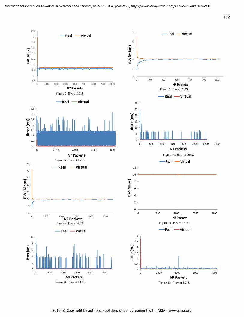
112



Figure 5. BW at 1518.

Figure 6. Jitter at 1518.







5,0

7,0

9,0

11,0

13,0

15,0

17,0

19,0

21,0

23,0

0 1000 2000 3000 4000 5000 6000 7000 8000

BW (M

bps)

Nº Packets

Real Virtual

0

0,5

1

1,5

2

2,5

3

3,5

0 2000 4000 6000 8000

Jitte

r (m

s)

Nº Packets

Real Virtual

0

5

10

15

20

25

30

35

0 500 1000 1500 2000 2500

BW (M

bps)

Nº Packets

Real Virtual

0

2

4

6

8

10

0 500 1000 1500 2000 2500

Jitte

r (m

s)

Nº Packets

Real Virtual

0

5

10

15

20

25

0 200 400 600 800 1000 1200

BW

(Mbp

s)

Nº Packets

Real Virtual

0

5

10

15

20

25

30

0 200 400 600 800 1000 1200 1400

Jitt

er (m

s)

Nº Packets

Real Virtual

0

2

4

6

8

10

12

0 2000 4000 6000 8000

BW

(Mb

ps

)

Nº Packets

Real Virtual

0

0,5

1

1,5

2

2,5

3

0 2000 4000 6000 8000

Jitte

r (m

s)

Nº Packets

Real Virtual

113




values of the real topology and the values obtained in the virtual topology. The data have similar values for both topologies, when the transmission was stabilized. Although in real topology is less than in virtual topology. The mean value of bandwidth in real topology is 9.9 Mbps while for virtual topology is 10 Mbps. The maximum values for real and virtual topology are the same 10 Mbps. The minimum values for real topology and virtual topology are different 9.8 Mbps and 9.9 Mbps.

In Figure 14, we can see the jitter values of the real topology and the values obtained in the virtual topology. The values of the real topology are higher than the ones of the virtual topology. The mean value of jitter in real topology is 0.019 ms while for virtual topology is 0.004 ms. The maximum values for real topology and virtual topology are different, 3.433 ms and 0.898 ms. The minimum values for real topology and virtual topology are the same, 0 ms. This section shows the results obtained in both cases, when traffic is being delivered over the network and in the virtual topology using Mininet.

c) MTU - 7999 In Figure 15, we can see the bandwidth consumption

values of the real topology and the values obtained in the virtual topology. The data have similar values for both topologies, when the transmission was stabilized.. The mean value of bandwidth in real and virtual topology is 10 Mbps. The maximum and minimum values for real topology and virtual topology are the same, 10 Mbps for maximum and 9,9 Mbps for minimum.

In Figure 16, we can see the jitter values of the real topology and the values obtained in the virtual topology. The values of the real topology are higher than the ones of the virtual topology. The mean value of jitter in real topology is 0.021 ms while for virtual topology is 0.005 ms. The maximum values for real topology and virtual topology are different, 1.177 ms and 1.756 ms. These values occurred at the very beginning and the virtual peak hide the one related with the real topology. The minimum values for real topology and virtual topology are the same, 0 ms.

Sending less traffic than the maximum bandwidth available seems that introduces less discrepancy between the virtual topology and the real one.



values of the real topology and the values obtained in the virtual topology. The data have similar values for both topologies, when the transmission was stabilized, although in real topology is less than in virtual topology. The mean value of bandwidth in real topology is 96 Mbps while for virtual topology is 100 Mbps. The maximum and minimum values for real topology and virtual topology are different, 100 Mbps and 101 Mbps for maximum and 94.3 Mbps and 7.3 Mbps for minimum.

In Figure 18, we can see the jitter values of the real topology and the values obtained in the virtual topology. The values of the real topology are higher than then ones of the virtual topology. The mean value of jitter in real topology is 0.011 ms while for virtual topology is 0.001 ms. The maximum values for real topology and virtual topology are different, 0.25 ms and 3.26 ms. The minimum values for real topology and virtual topology are the same, 0 ms.


values of the real topology and the values obtained in the virtual topology. The data have similar values for both topologies, when the transmission was stabilized, although in real topology is less than in virtual topology. The mean value of bandwidth in real topology is 98.559 Mbps while for virtual topology is 100 Mbps. The maximum and minimum values for real topology and virtual topology are different, 100 Mbps and 120.344 Mbps for maximum and 95.474 Mbps and 99.931 Mbps for minimum. Once again, the virtual topology is not providing realistic bandwidth values at the beginning of the transmission. But also, after transmitting a few packets the bandwidth values are similar to those from the real network.

In Figure 20, we can see the jitter values of the real topology and the values obtained in the virtual topology. The values of the real topology are higher than the ones of the virtual topology. The mean value of jitter in real topology is 0.017 ms while for virtual topology is 0 ms. The maximum values for real topology and virtual topology are different, 0,908 ms and 0.028 ms. The minimum values for real topology and virtual topology are the same, 0 ms.

114











0

2

4

6

8

10

12

0 500 1000 1500 2000 2500

BW (M

bps)

Nº Packets

Real Virtual

0,000

0,500

1,000

1,500

2,000

2,500

3,000

3,500

4,000

0 500 1000 1500 2000 2500

Jitte

r (m

s)

Nº Packets

Real Virtual

0

2

4

6

8

10

12

0 500 1000 1500

BW (M

bps)

Nº Packets

Real Virtual

0,000

0,500

1,000

1,500

2,000

0 500 1000 1500

Jitte

r (m

s)

Nº Packets

Real Virtual

0

20

40

60

80

100

120

140

0 5000 10000 15000 20000 25000 30000

BW (M

bps)

Nº Packets

Real Virtual

0,000

0,500

1,000

1,500

2,000

2,500

3,000

3,500

0 5000 10000 15000 20000 25000 30000

Jitte

r (m

s)

Nº Packets

Real Virtual

0

20

40

60

80

100

120

140

0 5000 10000 15000 20000 25000 30000

BW (M

bps)

Nº Packets

Real Virtual

0,000

0,200

0,400

0,600

0,800

1,000

0 5000 10000 15000 20000 25000 30000

Jitte

r (m

s)

Nº Packets

Real Virtual

115




Figure 22. Jitter at 7999.MTU - 7999

This section shows the results obtained in both cases, when traffic is being delivered over the network and in the virtual topology using Mininet.

In Figure 21, we can see the bandwidth consumption values of the real topology and the values obtained in the virtual topology. The data have similar values for both topologies, when the transmission was stabilized. The mean value of bandwidth in real topology is 98.911 Mbps while for virtual topology is 100 Mbps. The maximum and minimum values for real topology and virtual topology are different, 99.502 Mbps and 113.581 Mbps for maximum and 67.687 Mbps and 100 Kbps for minimum (due to the initial interval that some devices need to start sending messages). As previously, virtual topology is not providing realistic bandwidth values at the beginning of the transmission.

In Figure 22, we can see the jitter values of the real topology and the values obtained in the virtual topology. The values of the real topology are higher than the ones of the virtual topology. The mean value of jitter in real topology is 0.016 ms while for virtual topology is 0 ms. The maximum values for real topology and virtual topology are different, 0.749 ms and 0.123 ms. The minimum values for real topology and virtual topology are the same, 0 ms.

These lasts measurements indicate that the virtual topology can consume more bandwidth than the available in the real network.

V. CONCLUSION In this paper, we have studied the performance of virtual

networks and compared with real networks. For this study, we have transmitted packets with different MTU sizes, which correspond to Ethernet, FDDI, and WLAN 802.11 (also Jumbo Ethernet frames) packets and we have used different link capabilities and traffic through the network. It can be seen that the variation of the bandwidth between the real and virtual topologies are very low. However, in virtual networks, the first packets are usually sent with an unreal bandwidth. The results obtained for the jitter show that there are major deviations, although, we are working with a very low time scale, as we are dealing with milliseconds. In our future work, we will compare real and virtual networks using more complex topologies, and with Openflow compatible equipment.

ACKNOWLEDGMENT This work has been supported by the “Ministerio de

Economía y Competitividad”, through the “Convocatoria 2014. Proyectos I+D - Programa Estatal de Investigación Científica y Técnica de Excelencia” in the “Subprograma Estatal de Generación de Conocimiento”, Project TIN2014-57991-C3-1-P and the “Programa para la Formación de Personal Investigador – (FPI-2015-S2-884)” by the “Universitat Politècnica de València”.

REFERENCES [1] J. M. Jimenez, O. Romero, A. Rego, A. Dilendra, J. Lloret,

Performance Study of a Software Defined Network Emulator, The Eleventh International Conference on Internet Monitoring and Protection (ICIMP 2016), May 22 - 26, 2016 - Valencia, Spain

[2] Omnet++. Available at https://omnetpp.org/ [Last access November 8, 2016]

[3] OPNET is now part of Riberved. Available at http://es.riverbed.com/products/performance-management-control/opnet.html / [Last access November 8, 2016]

[4] The Network Simulator - ns-2. Available at http://www.isi.edu/nsnam/ns/ [Last access November 8, 2016]

[5] NS-3. Available at NS-3 website: https://www.nsnam.org/ [Last access November 8, 2016]

[6] NetSim NETWORK SIMULATOR. Available at http://www.boson.com/netsim-cisco-network-simulator [Last access November 8, 2016].

[7] GNS3 The software that empowers networks professionals. Available at https://www.gns3.com/ [Last access November 8, 2016].

[8] Software-Defined Networking: A Perspective from within a Service Provider Environment. Available at: https:// tools.ietf.org/pdf/rfc7149.pdf [Last access November 8, 2016]

[9] Liboftrace. Available at http://archive.openflow.org/wk/index .php/Liboftrace [Last access November 8, 2016]

[10] OFLOPS. Available at https://www.sdxcentral.com/projects/ oflops/ [Last access November 8, 2016]

[11] OpenSeer. Available at http://archive.openflow.org/wk/ index.php/OpenSeer [Last access November 8, 2016]

[12] What are SDN Controllers (or SDN Controllers Platforms)?. Available at https://www.sdxcentral.com/resources/sdn/sdn-controllers/[Last access November 8, 2016]

0

20

40

60

80

100

120

0 2000 4000 6000 8000 10000 12000 14000 16000

BW (M

bps)

Nº Packets

Real Virtual

0,000

0,100

0,200

0,300

0,400

0,500

0,600

0,700

0,800

0 2000 4000 6000 8000 10000 12000 14000 16000

Jitte

r (m

s)

Nº Packets

Real Virtual

116



[13] OpenFlow network virtualization with FlowVisor. Available at https://www.os3.nl/_media/2012-2013/courses/rp2/p28_ report.pdf [Last access November 8, 2016]

[14] OpenFlow switch. Available at http://searchsdn.techtarget. com/definition/OpenFlow-switch [Last access November 8, 2016]

[15] Mininet An Instant Virtual Network on your Laptop (or other PC). Available at http://mininet.org [Last access November 8, 2016]

[16] EstiNet Technologies Inc. Available at EstiNet Technologies website: http://www.estinet.com/index.php [Last access November 8, 2016].

[17] J. M. Jimenez, O. Romero, A. Rego, A. Dilendra and J. Lloret, “Study of Multimedia Delivery over Software Defined Networking”, in Network Protocols and Algorithm, vol. 7, No. 4, 2015, pp. 37-62, 2015, doi:10.5296/npa.v7i48794

[18] D. Kreutz, F. M. V. Ramos, P. Esteves Verissimo, C. Esteve Rothenberg, S. Azodolmolky, and S. Uhlig, "Software-Defined Networking: A Comprehensive Survey", Proceedings of the IEEE, Volume103, Issue 1, Jan. 2015, pp. 14-76, 2015, http://dx.doi.org/10.1109/JPROC.2014.2371999

[19] K. A. Noghani and M. O. Sunay, “Streaming Multicast Video over Software-Defined Networks”, Proceedings of the IEEE 11th International Conference on Mobile Ad Hoc and Sensor Systems (MASS) (2014), 28-30 Oct. 2014, pages 551-556, 2014, doi: 10.1109/MASS.2014.125

[20] H. Nam, K. Kim, J. Y. Kim and H. Schulzrinney, “Towards QoE-aware Video Streaming using SDN”, Global Communications Conference (GLOBECOM), Dec. 2014, pp 1317-1322, 2014, doi: 10.1109/GLOCOM.2014.7036990

[21] H. E. Egilmez, S. T. Dane, K. Tolga Bagci and A. Murat Tekalp, “OpenQoS: An OpenFlow controller design for multimedia delivery with end-to-end Quality of Service over Software-Defined Networks”, Signal & Information Processing Association Annual Summit and Conference (APSIPA ASC), 2012 Asia-Pacific, 3-6 Dec. 2012, Hollywood (USA), pp 1-8, 2012

[22] H. E. Egilmez, and A. M. Tekalp, ”Distributed QoS Architectures for Multimedia Streaming Over Software Defined Networks”, Multimedia, IEEE Transactions on , Volume:16 , Issue: 6 , Sept. 2014, pages: 1597 – 1609, 2014; doi:10.1109/TMM.2014.2325791

[23] A. Kassler, L. Skorin-Kapov, O. Dobrijevic, M. Matijasevic, and P. Dely, “Towards QoE-driven Multimedia Service Negotiation and Path Optimization with Software Defined Networking”, Software, Telecommunications and Computer Networks (SoftCOM), IEEE, Sept. 2012, Split (Croatia), pages: 1-5, 2012, ISBN: 978-1-4673-2710-7

[24] H. Yang, J. Zhang, Y. Zhao, Y. Ji, J. Han, Y. Lin, S. Qiu, Y. Lee, Time-aware Software Defined Networking for OpenFlow-based Datacenter Optical Networks, Network Protocols and Algorithms, Vol 6, No 4 (2014). pp. 77-91.

[25] M. Dramitinos, N. Zhang, M.. Kantor, J. Costa-Requena, I. Papafili, “Video Delivery over Next Generation Cellular Networks”, Network and Service Management (CNSM), 2013 9th International Conference, IEEE, 14-18 Oct. 2013, Zurich

(Switzerland), pp. 386-393, doi> 10.1109/CNSM.2013.6727862t

[26] R. L. S. de Oliveira, A. A. Shinoda, C. M. Schweitzer, L. Rodrigues Prete, “Using Mininet for Emulation and Prototyping Software-Defined Networks”, Communications and Computing (COLCOM), 2014 IEEE Colombian Conference, IEEE, 4-6 June 2014, Bogota (Colombia), pp. 1 - 6, DOI 10.1109/ColComCon.2014.6860404

[27] P. Wette, M. Dräxler, A. Schwabe, F. Wallaschek, M. H. Zahraee, H. Karl, “MaxiNet: Distributed Emulation of Software-Defined Networks”, Networking Conference, 2014 IFIP, 2-4 June 2014, Throndheim (Norway), pp. 1-9, DOI 10.1109/IFIPNetworking.2014.6857078

[28] A. V. Akella, K. Xiong, “Quality of Service (QoS) Guaranteed Network Resource Allocation via Software Defined Networking (SDN)”, Dependable, Autonomic and Secure Computing (DASC), 2014 IEEE 12th International Conference, 24-27 Aug. 2014, IEEE, Dalian (China), pp. 7-13, DOI 10.1109/DASC.2014.11.

[29] Z. Jingjing, C. Di, W. Weiming, J. Rong, W. Xiaochun, “The Deployment of Routing Protocols in Distributed Control Plane of SDN”, in The Scientific World Journal, Volume 2014, Article ID 918536, 8 pages, http://dx.doi.org/10.1155/2014/918536

[30] S. Salsano, N. Blefari-Melazzi, A. Detti, G. Morabito, L. Veltri, “Information centric networking over SDN and OpenFlow: Architectural aspects and experiments on the OFELIA testbed”, Computer Networks, Volume 57, Issue 16, 13 November 2013, pp. 3207-3221, DOI 10.1016/j.comnet.2013.07.031

[31] M. Gerola, R. Doriguzzi Corin, R. Riggio, F. De Pellegrini, E. Salvadori, H. Woesner, T. Rothe, M. Suñé, L. Bergesio, “Demonstrating in ter-testbed network virtualization in OFELIA SDN experimental facility”, Computer Communications Workshops (INFOCOM WKSHPS), 2013 IEEE Conference, 14-19 April 2013, Turin (Italy), pp. 39-40, DOI 10.1109/INFCOMW.2013.6970724

[32] S.-Y. Wang, C.-L. Chou, C.-M. Yang, “EstiNet OpenFlow Network Simulator and Emulator”, in Communications Magazine, IEEE (Volume:51 , Issue: 9 ), IEEE, September 2013, pp. 110-117, DOI 10.1109/MCOM.2013.6588659

[33] S.-Y. Wang, “Comparison of SDN OpenFlow Network Simulator and Emulators: EstiNet vs. Mininet”, in Computers and Communication (ISCC), 2014 IEEE Symposium, 23-26 June 2014, Funchal (Portugal), pp 1-6, DOI 10.1109/ISCC.2014.6912609

[34] Cisco Catalyst 3560 Series Switches Data Sheet. Available at Cisco website: http://www.cisco.com/c/en/us/products/ collateral/switches/catalyst-3560-series-switches/product_ data_sheet09186a00801f3d7d.html [Last access January 14, 2016]

[35] Wireshark software. Available at Wireshark website: https://www.wireshark.org/ [Last access January 14, 2016]

[36] Terminology for Benchmarking Network-layer Traffic Control Mechanisms. Available at https://www.ietf.org/rfc/rfc4689.txt.txt [Last access January 14, 2016]

www.iariajournals.org

International Journal On Advances in Intelligent Systems

issn: 1942-2679

International Journal On Advances in Internet Technology

issn: 1942-2652

International Journal On Advances in Life Sciences

issn: 1942-2660

International Journal On Advances in Networks and Services

issn: 1942-2644

International Journal On Advances in Security

issn: 1942-2636

International Journal On Advances in Software

issn: 1942-2628

International Journal On Advances in Systems and Measurements

issn: 1942-261x

International Journal On Advances in Telecommunications

issn: 1942-2601

The - IARIA Journals · Mario Freire, University of Beira Interior, Portugal Carlos Becker...

Documents

Transcript of The - IARIA Journals · Mario Freire, University of Beira Interior, Portugal Carlos Becker...