The house edge and play time: Do industry heuristics ...

The House Edge and Play Time:Do Industry Heuristics Fairly

Describe This Relationship?

Anthony LucasA.K. Singh

AbstractBased on modified versions of licensed pay tables from reel slot machines, simulations ofplay failed to indicate a statistically significant difference in the spins per losing player(SPLP), despite a marked difference in the pars (i.e., 7.9% vs. 12.9%). To reflect a volumeof play consistent with frequent gambling, the simulations included results from 1–4 vis-its per week, for the equivalent of one year. Additionally, this level of play was repeatedfor 100 “years,” within multiple scenarios of buy-in amounts and stoppage-of-play criteria.Still, most outcomes indicated a negligible decline in SPLP, in spite of the 63%-increase inthe par. These results were reproduced from a second pairing of games featuring a 117%-increase in par (i.e., 4.6% vs. 10.0%). The findings spotlighted considerable limitations ofpopular industry heuristics related to the relationship between par and play time. While ad-ditional studies are warranted, the outcomes suggested that operators may be overly mind-ful of the fallout from increased pars. These overbroad beliefs are likely to impede criticalprogress toward revenue optimization.

Anthony LucasUniversity of Nevada,

Las [email protected]

A.K. SinghUniversity of Nevada,

Las [email protected]

AcknowledgmentsThis work was supported by a research grant from the William F. Harrah College of Hospitality at the Universityof Nevada, Las Vegas.

UNLV Gaming Research & Review Journal � Volume 25 (2021) Paper 2 13

mailto:[email protected]

mailto:[email protected]

IntroductionSlots are critical to the success of most casinos, but they often take on an exaggerated

importance for Western-market operators catering to a frequently-visiting clientele. Whilethere are some obvious and notable exceptions in Asia, the majority of casinos are heavilyreliant on profits from slot machines. Therefore, much attention is given to the managementof these complex devices. At the center of this attention is the role of par in the customerexperience. Par represents the machine’s programmed, long-run, house advantage. Unlikenearly all consumer products and services, this “price” is not marked on reel slots. Andthere is much debate related to the ability of gamblers to infer reel pars from play alone.Typically, the bulk of slot revenue comes from reel games, hence the increased level ofconcern for par/price detection.

Many operators and gaming insiders have sternly cautioned against the fallout fromincreasing pars (Frank, 2017; Gallaway, 2014; Hwang, 2019; Legato, 2019), but resultsfrom a series of recent field studies found increased pars to consistently produce greatergame-level revenues (Lucas & Spilde, 2020b). Still, some have argued that any such gainscome at the expense of the individual gambler’s experience, contending that clear declinesin play time would be inevitable (Hwang, 2019; Legato, 2019; Meczka, 2017; Wyman,2020). Their primary concern is that frequent players will eventually notice that theirbankroll does not last as long as it once did.

This study aims to better understand how increases in par affect the individual gam-bler’s play time, ceteris paribus. Given the remarkable amount of variance in the outcomedistribution of modern slot machines, along with the wallet- and time-related limitationsof gamblers, this is far from settled science. The game-level results from the aforemen-tioned field studies represent a key performance measure for operators, but they comprisemany individual experiences. And it is possible for these individual contributions to vary.The current study shifts the focus from the collective clientele to the individual gambler,providing a deeper understanding of the impact of par on the gaming experience.

Our results will inform operators who want to further assess the ramifications of in-creased pars, and manufacturers who wish to design games that produce player experiencesthat are in step with the needs of casino operators. Academically, the findings will add toa growing literature on how the mathematical parameters of slot machine pay tables affectthe player experience. Additionally, we examine the extent to which samples generated byindividual players serve as valid proxies for known population parameters, through the lensof Tversky and Kahneman’s (1971) Law of Small Numbers. Ultimately, these ends willallow for an objective evaluation of popular industry heuristics related to par and the playerexperience.

Literature ReviewIndustry Positions

Industry pundits, consultants, and operators have often conflated the long-term andshort-term effects of par, usually failing to recognize the context of the individual gambler’sexperience (Frank, 2017; Gallaway, 2014; Hwang, 2019; Legato, 2015, 2019; Meczka,2017; Tottenham, 2019; Wyman, 2020). This is understandable, as management is com-fortable with and afforded many aggregated and/or long-term views of slot machine results.For example, one popular heuristic that is advanced as support for the short-term effects ofpar holds that a game with a 5% par can be expected to provide twice the average play timeof a game with a 10% par, ceteris paribus. The following example reveals the assumptionsthat underlie this conclusion: (1) Game A has a 5% par; (2) Game B has a 10% par; (3)a player engages each of these two games with a fixed bankroll (e.g., $100); and (4) theplayer places equal and constant wagers on both games until she loses her entire initialbankroll. In short, this argument hinges on the following simple equations: (1) Game A:$100/0.05 = $2,000 in total wagers; and (2) Game B: $100/0.10 = $1,000 in total wagers.Therefore, subscribers conclude that Game A can be expected to provide twice the playtime as Game B, based on the difference in total wagers (i.e., coin-in).

14 UNLV Gaming Research & Review Journal � Volume 25 (2021) Paper 2

The House Edge and Play Time

Of course, not all players wager until they lose their entire buy in, and the games donot take a constant percentage of each wager – far from it. That is, this argument assumesa geometric distribution of outcomes and a mandatory bankruptcy condition. The formerdoes not reflect how slot machines work and the latter assumes that no players win, or walkwith any credits. The problem here is that games are not experienced in the long term. Tothe contrary, they are experienced in the extreme short term. Given the amount of variancein the outcome distribution of modern reels, even considerable differences in pars (i.e.,population means) can be difficult to detect for an individual player (Singh et al., 2013).This is an issue of contextual congruency, as in viewing the short-term experience throughthe lens of long-run expectations.

Similarly, in his review of the related research, Hwang (2019) cited elevated wager-ing volume as a clear marker of differences in pars, but his game-level coin-in estimateswere based on shortcut, long-term math that failed to separate the outcomes produced bywinners from those generated by losers. It is important to note that the winning playershave the capacity to generate disproportionate coin-in, from recycling jackpots (i.e., housemoney). Moreover, we contend that it is the losing players who would be most likely toinvoke abstract measures of gaming value, such as play time. Therefore, it is critical toisolate the results of the losing players when attempting to understand measures of playtime, also known as time on device (TOD). From the perspective of the individual player,game-level aggregation of results obscures this important distinction.

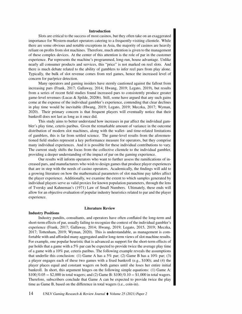
Figure 1 was constructed to summarize the views and concerns reflected in the pre-viously cited trade literature. This figure is helpful in establishing the need for the currentstudy, as our focus was on understanding the extent to which the individual gambler’s playtime is affected by changes in pars. This aim represents the crux of Figure 1, as all of thepotential consequences and concerns related to increased pars stem from the assumption ofnoticeably decreased play time. It is important to limit the applicability of Figure 1 to mar-kets that are characterized by a frequently-visiting clientele; as such concerns are muted indestination markets like the Las Vegas Strip.

Figure 1A framework for examining popular industry positions on par and the reel slot player ex-perience in repeater markets.

In short, Figure 1 depicts the belief that increased pars will lead to noticeable differ-ences in play time, which will in turn lead to increases in negative word of mouth amongplayer populations. The increased negative WOM is thought to increase brand damage,resulting in declines in future slot win. Following the lower path of Figure 1, it is also be-lieved that noticeable decreases in play time will lead to fewer visits from existing players,further reducing future slot win.

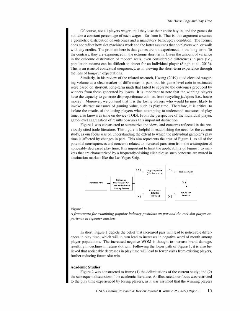
Academic StudiesFigure 2 was constructed to frame (1) the delimitations of the current study; and (2)

the subsequent discussion of the academic literature. As illustrated, our focus was restrictedto the play time experienced by losing players, as it was assumed that the winning players


would be satisfied by their outcome. Within this limited domain, we examined the studiesthat have addressed the play-time impacts of each variable appearing within the dotted-linebox. Figure 2 is not offered as a valid model of the reel slot player’s experience, but ratheras a framework for the literature review.

Figure 2A framework for discussing satisfaction with the reel slot player’s experience.

As shown, Figure 2 assumes that the effect of each variable within the dotted-line boxis considered under the assumption that all other potential sources of impact on play timeare held constant. Of course, variables other than play time could also affect the satisfactionlevel of losing players, yet it remains as the primary concern among industry insiders.

Hit Frequency & Play Time. Kilby and Fox (1997) sought to examine the then-popular notion that hit frequency was a primary driver of play time. Play was simulated on10 reel slot machines, attempting to hold par constant. A total of 100,000 players wageredunder fixed simulation constraints, on each of the 10 games. These virtual players engagedthe games under the following three scenarios: (1) Start with 100 credits and wager untilreaching 200 credits, or bankruptcy; (2) Start with 100 credits and wager until reaching 300credits, or bankruptcy; and (3) Start with 200 credits and wager until reaching 400 credits,or bankruptcy. The results from losing players were separated from those produced by thewinners, permitting the calculation of mean spins per losing player (i.e., SPLP) for eachgame. The results clearly failed to support a positive and monotonic relationship betweenhit frequency and play time. In hindsight, this was a logical result, as the hit frequencycalculation ignores hit magnitude. For instance, its computation treats/considers a top-award jackpot the same as a single-credit payout. Laudable contributions from this workincluded establishing winning and losing players under real-world engagement criteria, andisolating the results of the losing players.

Standard Deviation & Play Time. Lucas, Singh and Gewali (2007) extended Kilbyand Fox (1997) by examining the relationship between pay table variance and SPLP. Specif-ically, they observed a monotonic relationship between the standard deviation of the paytable and SPLP. As the standard deviation increased, SPLP was found to decrease. Thisresult was produced by simulating play on six different reel games, with the pars held con-stant at 10%. The standard deviations ranged from 2.37 coins to 12.21 coins. The playerengagement criteria were identical to those employed in Kilby and Fox (1997). The resultsfrom Lucas et al. held across all three of Kilby and Fox’s engagement conditions.

Lucas and Singh (2008) simulated play on five, reel games with Game 1 offering apar of 11.20% and a standard deviation of 2.37 coins, and Game 5 featuring a par of 5.60%and a standard deviation of 7.21 coins. The par incrementally decreased by approximately1.5 percentage points from Game 1 to Game 5, while the standard deviation incrementallyincreased by approximately 1.2 coins. Fifty thousand virtual players engaged each of the



five games, with each one beginning with 200 credits and wagering until bankrupt, orreaching at least 400 credits. The greatest mean SPLP was generated by Game 1, i.e., thegame with greatest par. In fact, the results were monotonic, with decreases in par resultingin decreases in SPLP. This result confounded the general applicability of the relationshipbetween par and play time, as described in the trade literature (Frank, 2017; Hwang, 2019,Legato, 2019; Meczka, 2019; Tottenham, 2019; Wyman, 2020). Specifically, lower pars donot necessarily result in greater play time.

Par & Play Time. A simple example from Kilby and Fox (1997) demonstrated thesevere limitations of the argument that lower pars on reel games must result in greater playtime. They described a hypothetical reel slot that consisted of 254 blanks and one jackpotsymbol, on each of four reels. The payout schedule was simple, consisting of a singleline indicating a payout of 4,224,022,374 credits, for the only possible jackpot. This gamefeatured 4,228,250,625 possible outcomes (i.e., 2554). Given a one-credit wager on eachspin, the game would produce a payback percentage of 99.9% (i.e., a 0.1% par). While thisgame features a remarkably low par, how much play time would you expect it to produce?How many players would call this game loose? It would very likely be the game with theleast mean SPLP of any slot machine on the floor. Again, we cannot conclude that lowerpars necessarily result in greater play time. Although this is an extreme example, it shouldraise some red flags for subscribers to the popular heuristic of low pars produce noticeablygreater play time.

Staying with the previous example, consider the outcomes produced by 10,000 play-ers who engage the 99.9% payback game with a $100 bankroll, and wager $1 per spin.In terms of the average number of spins, wouldn’t you expect all of them to lose everyspin? That is, the mean, median, and mode number of spins would all equal 100. Afterall, the only jackpot is expected to hit once in every 4.2 million spins. Even if one playerwere lucky enough to hit the jackpot, the median and mode number of spins would still be100. But if you invoke the math advanced by the industry experts (Legato, 2019; Meczka,2017; Hwang, 2019, Wyman, 2020), then you would expect the mean number of spins tobe 100,000 (i.e., $100/0.001/$1). Of course, this would require (1) someone to hit the jack-pot; and (2) continue play until losing all of the jackpot credits to the game. Even then, themean number of spins would be heavily influenced by the lone winner. And it would seemreasonably safe to assume that this is the one player who would already be satisfied withher experience.

Still, to the best of our knowledge, there have been no published studies isolatingthe impact of par on play time, under gaming conditions reflective of actual play, on paytables resembling actual games. Within this general domain, Harrigan and Dixon (2010)conducted simulations designed to compare variables such as the total number of spins perplayer. They simulated play on two, reel slots, with one par set at 2% and the other at 15%.While they did see significant increases in the mean number of spins on the 2% game, theeffect diminished when they examined the median outcomes. They were careful to notethis difference in their results. But their simulation required the virtual players to makeconstant wagers until going bankrupt. This condition forced the relatively few winners toplay-off considerable credit balances, hence the difference in their results (i.e., betweenmeans and medians). That is, the origin of the significant differences in the means seemedto stem from requiring the outliers (i.e., those who hit jackpots) to wager their credits untilreaching a zero balance.

Dixon et al. (2013) and Lucas and Singh (2011) also conducted studies on the differ-ences in outcomes produced by games with different pars. Although Dixon et al. conducteda lab study with live gamblers and Lucas and Singh simulated play, both studies fixed thenumber of spins on each of the paired reel games. In the case of Dixon et al., their aim wasto determine whether players could identify the lower par game, after equal play on both a2% game and a 15% game. For Lucas and Singh, it was to determine whether the differ-ent pars on otherwise identical games would produce significantly different results, givenequal play on both games. Dixon et al. reported that all 7 of the subjects who completed


their study were able to identify the low-par game. Lucas and Singh found a paucity ofsignificant differences in the outcomes of their paired games, but their pairings featured amaximum difference of 9 percentage points (vs. 13 for Dixon et al.). On balance, the re-sults from Lucas and Singh suggested there was no significant difference in the outcomes,despite the difference in pars. By eliminating the fixed-number-of-spins constraint, thecurrent study seeks to identify whether games with different pars will produce significantlydifferent SPLP results.

In a related research stream, a series of field studies produced results that failed tosupport the ability of players to detect differences in the pars of otherwise identical games(Lucas & Spilde, 2019a, 2019b, 2020a, 2020b). This conclusion was based on a failure toobserve play migration from the high-par games to the low-par games, despite the nearbylocation of the paired low-par games. Moreover, the majority of these results were observedover 180- to 365-day sample periods, in casinos that were heavily reliant on a frequently-visiting clientele. Additionally, the high-par games produced significantly greater revenuesthat were sustained over these sample periods. These results also indicated an inabilityof the frequently-visiting clientele to detect (1) a price shock; and (2) an obvious gamingvalue. Regarding the latter, one study pitted a 4% penny reel against a 15% version of thesame game (Lucas & Spilde, 2020a). If players were able to detect pars from play alone,one would expect to see the 4% game demonstrate obvious performance gains, by nearlyall measures. This did not occur, in spite of the game’s unusually low par (i.e., for a pennyreel), over the course of a 365-day sample.

Cognitive BiasMany of the industry positions, as well as the results from academic studies, could

certainly be influenced by way of cognitive bias. Tversky and Kahneman’s (1971) face-tiously dubbed Law of Small Numbers is particularly germane to this issue. The authorsbase this “law” on something they refer to as the representation hypothesis, which is theo-rized to govern strongly-anchored yet inaccurate intuitions about chance. In their paper, theauthors demonstrate how even trained researchers overestimate the extent to which resultsfrom small samples represent population parameters. This is the very issue that underliesthe explanations of slot play offered by many industry operators, consultants, and pun-dits (Frank, 2017; Hwang, 2019; Meczka, 2017; Legato, 2019; Tottenham, 2019; Wyman,2020). That is, to what extent can we expect a gambler’s sample of randomly generatedoutcomes to reflect the population from which it came?

Tversky and Kahneman (1971) note the prevalence of beliefs in the representative-ness of random samples, regardless of sample size, or what sampling theory would predict.Further, they note and demonstrate how people tend to believe that every random sequenceof events must be reflective of the population parameters, even in remarkably small sam-ples/series. It follows that any sequence of outcomes that deviates from a known popula-tion parameter would be expected to quickly self correct, rather than slowly dissipate. Ofcourse, the gambler’s fallacy is the best known version of this bias; however, researchershave observed other similar forms in live gaming environments, including stock-of-luck,hot hand, and hot outcome (Croson & Sundali, 2005; Sundali & Croson, 2006). All ofthese biases stem from a belief in autocorrelation within a non-autocorrelated random se-quence of outcomes (Sundali & Croson, 2006).

Regarding the issue of play time, many seem to believe that a single player’s gam-bling activity will produce a sample of outcomes that would be generally sufficient to iden-tify changes in a game’s par, i.e., its true population parameter (Frank, 2017; Hwang, 2019;Meczka, 2017; Legato, 2019; Tottenham, 2019; Wyman, 2020). Granted, this sample couldbe produced over many visits. Still, with the considerable variance in the outcome distri-bution of the modern slot machine, this would likely require a larger-than-expected sample(Singh et al. 2013). In step with this concern, Tversky and Kahneman (1971) demonstratedthe tendency of people to overestimate the degree to which small samples are similar to



one another and to the population from which they were generated. With reel slots, even“large” samples may be too small.

HypothesesTo the best of our knowledge, no published studies have empirically examined and/or

demonstrated how differences in pars affect the number of spins experienced by losingplayers, assuming otherwise equal wagering parameters. These parameters were designedto reflect actual gaming behavior, with precise definitions found in the methodology sec-tion. With this end in mind, the following null hypothesis was advanced:

H0 : µ1i j−µ2i j = 0.

Within H0, µ1i j represented the mean number of spins produced by a losing player, on agame with par level 1, over i sessions of play, under j wagering parameters. µ2i j repre-sented the same for par level 2. For example, the mean SPLP from play on a 7.9% par wascompared against that from a 12.9% par, over 100 sessions of play on each game, wherea gambler placed constant wagers from a starting bankroll of 100 credits, and terminatedplay after reaching either 200 credits or bankruptcy. While the pars varied, the wageringparameters remained constant in all tests of the null. Further details are forthcoming in theMethodology section.

MethodologyThe Game

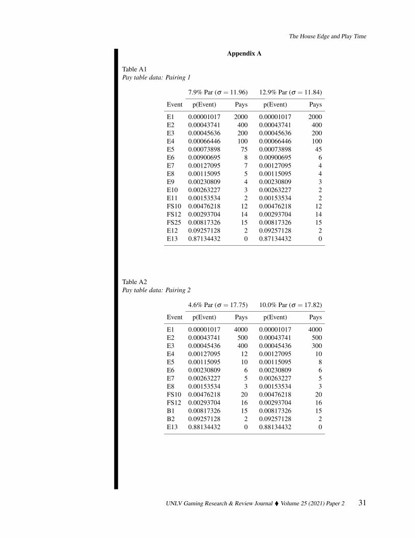
The initial simulations incorporated pay tables from two versions of the same garden-variety penny reel (See Appendix A, Table A1). For purposes of our research question wedid modify the two pay tables, attempting to maintain the general structure of the originalformats. We were not permitted to identify the title or manufacturer of the game, but we canreport that both par versions were licensed for distribution in multiple markets, includingNevada. Additionally, the original pay tables were available in multiple titles (i.e., the mathwas skinned). More specifically, the art, theme, and graphics differed across the titles, butthe game math and structure of play remained the same.

All licensed versions of this game included five, 50-70-stop reels, 40 pay lines, afree-spin feature, and a forced minimum wager of 60 credits per spin. Per the par sheet,the expected value was not affected by the amount wagered per line, or the number oflines played. No progressive jackpots were offered on either version of the game. Thetwo simulated versions featured pars of 12.9% and 7.9%, respectively. This differencerepresented a 63% increase in the par, from the level of the low-par game. The high-pargame was established at 12.9%, as the majority of penny pars range from 12% to 16%(Gallaway, 2014). Legato (2019) confirmed this position, noting the push to move beyondthe 12% mark. The low-par game was reduced by five percentage points, to produce thedesired par gap for this first look into the impact on SPLP.

The standard deviation was 11.96 credits for the 7.9% game, and 11.84 credits for the12.9% game. The direction and magnitude of this difference was reflective of the designedgame parameters from which operators must choose. That is, the standard deviations withinthe suite of licensed pars for a particular title are typically not held constant, often decliningvery slightly with increases in the par (Lucas & Spilde, 2019b). It was for this reason thatthis parameter was not held constant in the simulations, as the intent was to compare theresults from play under real-world game conditions.

The SimulationsAn individual gambler’s play on each of two par versions was simulated, holding

the following variables constant: Starting bankroll, wager per spin; number of gaming ses-sions on each version; termination criteria; and the number of experimental replications.


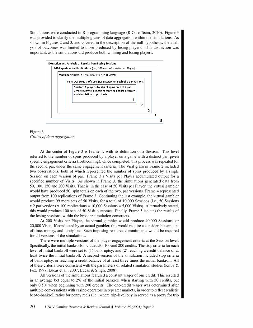
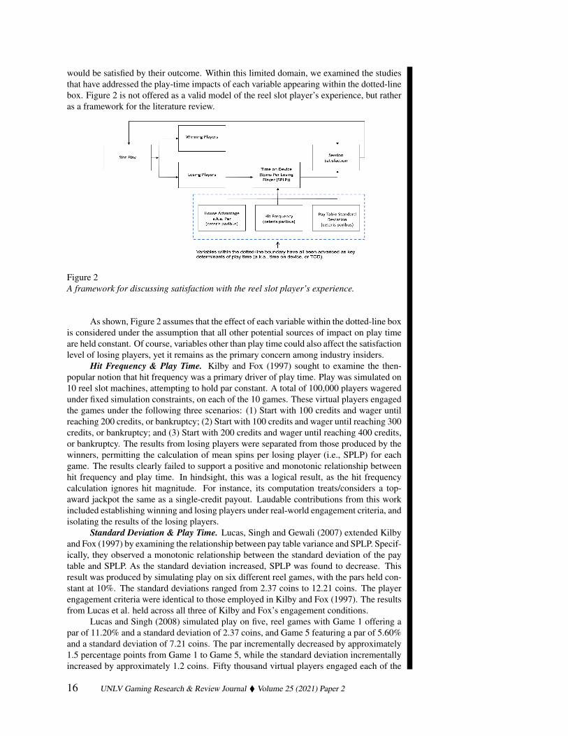
Simulations were conducted in R programming language (R Core Team, 2020). Figure 3was provided to clarify the multiple grains of data aggregation within the simulations. Asshown in Figures 2 and 3, and covered in the description of the null hypothesis, the anal-ysis of outcomes was limited to those produced by losing players. This distinction wasimportant, as the simulations did produce both winning and losing players.

Figure 3Grains of data aggregation.

At the center of Figure 3 is Frame 1, with its definition of a Session. This levelreferred to the number of spins produced by a player on a game with a distinct par, givenspecific engagement criteria (forthcoming). Once completed, this process was repeated forthe second par, under the same engagement criteria. The Visit grain in Frame 2 includedtwo observations, both of which represented the number of spins produced by a singleSession on each version of par. Frame 3’s Visits per Player accumulated output for aspecified number of Visits. As shown in Frame 3, the simulations generated data from50, 100, 150 and 200 Visits. That is, in the case of 50 Visits per Player, the virtual gamblerwould have produced 50, spin totals on each of the two, par versions. Frame 4 representedoutput from 100 replications of Frame 3. Continuing the last example, the virtual gamblerwould produce 99 more sets of 50 Visits, for a total of 10,000 Sessions (i.e., 50 Sessionsx 2 par versions x 100 replications = 10,000 Sessions = 5,000 Visits). Alternatively stated,this would produce 100 sets of 50-Visit outcomes. Finally, Frame 5 isolates the results ofthe losing sessions, within the broader simulation constructs.

At 200 Visits per Player, the virtual gambler would produce 40,000 Sessions, or20,000 Visits. If conducted by an actual gambler, this would require a considerable amountof time, money, and discipline. Such imposing resource commitments would be requiredfor all versions of the simulations.

There were multiple versions of the player engagement criteria at the Session level.Specifically, the initial bankrolls included 50, 100 and 200 credits. The stop criteria for eachlevel of initial bankroll were set to (1) bankruptcy; and (2) reaching a credit balance of atleast twice the initial bankroll. A second version of the simulation included stop criteriaof bankruptcy, or reaching a credit balance of at least three times the initial bankroll. Allof these criteria were consistent with the parameters of related simulation studies (Kilby &Fox, 1997; Lucas et al., 2007; Lucas & Singh, 2008).

All versions of the simulations featured a constant wager of one credit. This resultedin an average bet equal to 2% of the initial bankroll when starting with 50 credits, butonly 0.5% when beginning with 200 credits. The one-credit wager was determined aftermultiple conversations with casino operators in repeater markets, in order to reflect realisticbet-to-bankroll ratios for penny reels (i.e., where trip-level buy in served as a proxy for trip



bankroll). Our fixed wager was also in line with the average bet estimates for penny reels,as reported by repeater-market operators in Legato (2019), i.e., c. US$0.80 per spin.

Data AnalysisAll hypothesis testing was conducted by way of two-tailed, independent measures

t-tests. As recommend by Welch (1947), unequal variances were assumed. The alpha wasset at 0.05 for all hypothesis tests, but a Bonferroni Correction was necessary as the nullwas tested 100 times at each level of the engagement parameters. This resulted in an alphaof 0.0005 (i.e., 0.05/100). As the results of losing players were parsed from the larger setof outcomes, it did result in an unbalanced design. For example, at the simulation level of100 visits per player, a gambler could produce 82 losing visits on one par, and 84 on theother. The two-samples t-test from Welch, however, is known to perform well under suchconditions (McDonald, 2014).

From Figure 3, the Visits-per-Player levels were selected to represent the followingannual patronage patterns: 50 = 1 visit per week; 100 = 2 visits per week; 150 = 3 visitsper week; and 200 = 4 visits per week. It was assumed that play did not occur in 2 weeksof the year for reasons such as vacations, business travel, illness, or any other potentialinterruption of regular/normal visitation. These patronage levels were important, as resultsfrom frequent players have been cited as more likely to reveal differences in pars (Frank,2017; Meczka, 2017; Wyman, 2020). The simulations produced 100 tests of the null, aftera “year” of gambling, at each of these four levels of weekly visitation.

ResultsThere were 100 tests of each null, at each level of Visits per Player, for each set of

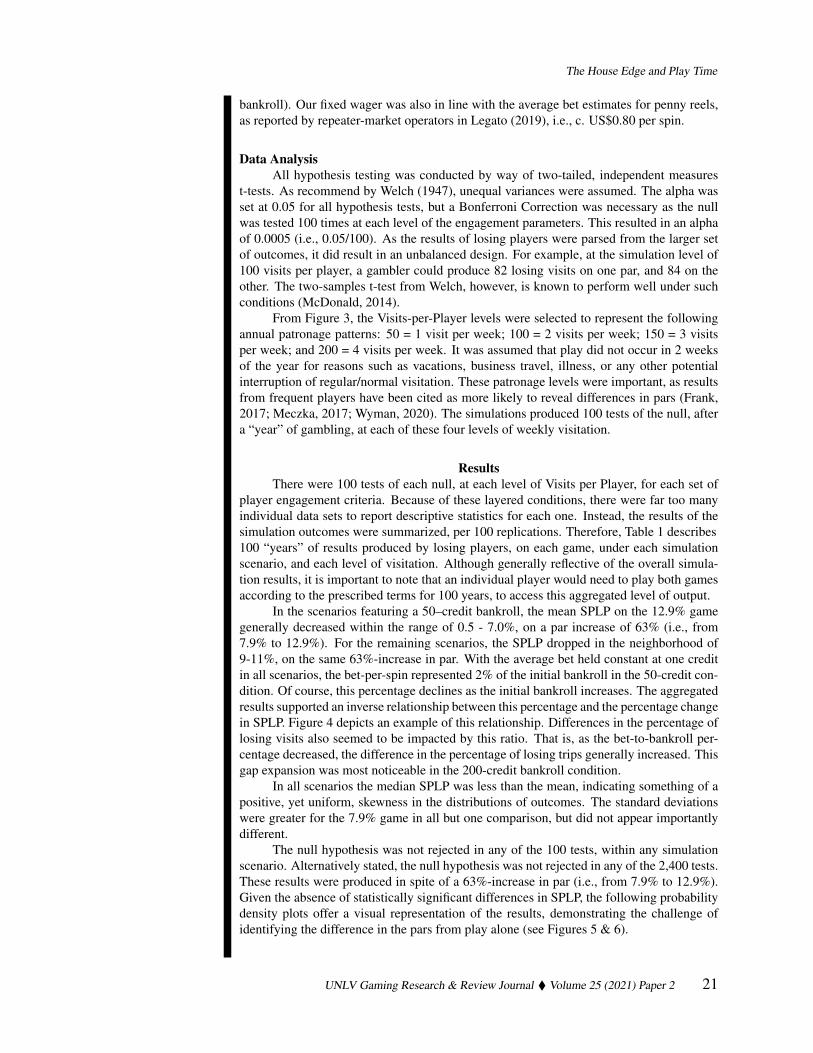
player engagement criteria. Because of these layered conditions, there were far too manyindividual data sets to report descriptive statistics for each one. Instead, the results of thesimulation outcomes were summarized, per 100 replications. Therefore, Table 1 describes100 “years” of results produced by losing players, on each game, under each simulationscenario, and each level of visitation. Although generally reflective of the overall simula-tion results, it is important to note that an individual player would need to play both gamesaccording to the prescribed terms for 100 years, to access this aggregated level of output.

In the scenarios featuring a 50–credit bankroll, the mean SPLP on the 12.9% gamegenerally decreased within the range of 0.5 - 7.0%, on a par increase of 63% (i.e., from7.9% to 12.9%). For the remaining scenarios, the SPLP dropped in the neighborhood of9-11%, on the same 63%-increase in par. With the average bet held constant at one creditin all scenarios, the bet-per-spin represented 2% of the initial bankroll in the 50-credit con-dition. Of course, this percentage declines as the initial bankroll increases. The aggregatedresults supported an inverse relationship between this percentage and the percentage changein SPLP. Figure 4 depicts an example of this relationship. Differences in the percentage oflosing visits also seemed to be impacted by this ratio. That is, as the bet-to-bankroll per-centage decreased, the difference in the percentage of losing trips generally increased. Thisgap expansion was most noticeable in the 200-credit bankroll condition.

In all scenarios the median SPLP was less than the mean, indicating something of apositive, yet uniform, skewness in the distributions of outcomes. The standard deviationswere greater for the 7.9% game in all but one comparison, but did not appear importantlydifferent.

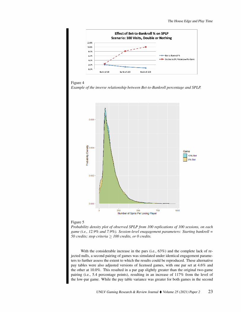
The null hypothesis was not rejected in any of the 100 tests, within any simulationscenario. Alternatively stated, the null hypothesis was not rejected in any of the 2,400 tests.These results were produced in spite of a 63%-increase in par (i.e., from 7.9% to 12.9%).Given the absence of statistically significant differences in SPLP, the following probabilitydensity plots offer a visual representation of the results, demonstrating the challenge ofidentifying the difference in the pars from play alone (see Figures 5 & 6).


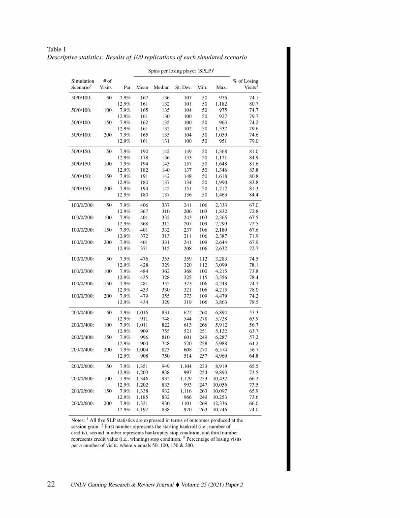
Table 1Descriptive statistics: Results of 100 replications of each simulated scenario

Spins per losing player (SPLP)1

Simulation # of % of LosingScenario2 Visits Par Mean Median St. Dev. Min. Max. Visits3

50/0/100: 50 7.9% 167 136 107 50 976 74.112.9% 161 132 101 50 1,182 80.7

50/0/100: 100 7.9% 165 135 104 50 975 74.712.9% 161 130 100 50 927 79.7

50/0/100: 150 7.9% 162 135 100 50 963 74.212.9% 161 132 102 50 1,337 79.6

50/0/100: 200 7.9% 165 135 104 50 1,059 74.612.9% 161 131 100 50 951 79.0

50/0/150: 50 7.9% 190 142 149 50 1,368 81.012.9% 178 136 133 50 1,171 84.9

50/0/150: 100 7.9% 194 143 157 50 1,648 81.612.9% 182 140 137 50 1,346 83.8

50/0/150: 150 7.9% 191 142 148 50 1,618 80.812.9% 180 137 134 50 1,990 83.8

50/0/150: 200 7.9% 194 145 151 50 1,712 81.312.9% 180 137 136 50 1,463 84.4

100/0/200: 50 7.9% 406 337 241 106 2,333 67.012.9% 367 310 206 103 1,832 72.8

100/0/200: 100 7.9% 401 332 243 103 2,365 67.512.9% 368 312 207 109 2,299 72.5

100/0/200: 150 7.9% 401 332 237 106 2,189 67.612.9% 372 313 211 106 2,387 71.9

100/0/200: 200 7.9% 401 331 241 109 2,644 67.912.9% 371 315 208 106 2,632 72.7

100/0/300: 50 7.9% 476 355 359 112 3,283 74.512.9% 428 329 320 112 3,099 78.1

100/0/300: 100 7.9% 484 362 368 100 4,215 73.812.9% 435 328 325 115 3,356 78.4

100/0/300: 150 7.9% 481 355 373 106 4,248 74.712.9% 433 330 321 106 4,215 78.0

100/0/300: 200 7.9% 479 355 373 109 4,479 74.212.9% 434 329 319 106 3,863 78.5

200/0/400: 50 7.9% 1,016 831 622 260 6,894 57.312.9% 911 748 544 278 5,728 63.9

200/0/400: 100 7.9% 1,011 822 613 266 5,912 56.712.9% 909 755 521 251 5,122 63.7

200/0/400: 150 7.9% 996 810 601 249 6,287 57.212.9% 904 748 520 258 5,988 64.2

200/0/400: 200 7.9% 1,004 823 608 270 6,574 56.712.9% 908 750 514 257 4,969 64.8

200/0/600: 50 7.9% 1,351 949 1,104 233 8,919 65.512.9% 1,203 838 997 254 9,893 73.5

200/0/600: 100 7.9% 1,346 932 1,129 253 10,432 66.212.9% 1,202 833 993 247 10,056 73.5

200/0/600: 150 7.9% 1,338 932 1,116 263 10,097 65.912.9% 1,185 832 966 249 10,253 73.6

200/0/600: 200 7.9% 1,331 930 1101 269 12,336 66.012.9% 1,197 838 970 263 10,746 74.0

Notes: 1 All five SLP statistics are expressed in terms of outcomes produced at thesession grain. 2 First number represents the starting bankroll (i.e., number ofcredits), second number represents bankruptcy stop condition, and third numberrepresents credit value (i.e., winning) stop condition. 3 Percentage of losing visitsper n number of visits, where n equals 50, 100, 150 & 200.



Figure 4Example of the inverse relationship between Bet-to-Bankroll percentage and SPLP.

Figure 5Probability density plot of observed SPLP from 100 replications of 100 sessions, on eachgame (i.e., 12.9% and 7.9%). Session-level enagagement parameters: Starting bankroll =50 credits; stop criteria ≥ 100 credits, or 0 credits.

With the considerable increase in the pars (i.e., 63%) and the complete lack of re-jected nulls, a second pairing of games was simulated under identical engagement parame-ters to further assess the extent to which the results could be reproduced. These alternativepay tables were also adjusted versions of licensed games, with one par set at 4.6% andthe other at 10.0%. This resulted in a par gap slightly greater than the original two-gamepairing (i.e., 5.4 percentage points), resulting in an increase of 117% from the level ofthe low-par game. While the pay table variance was greater for both games in the second


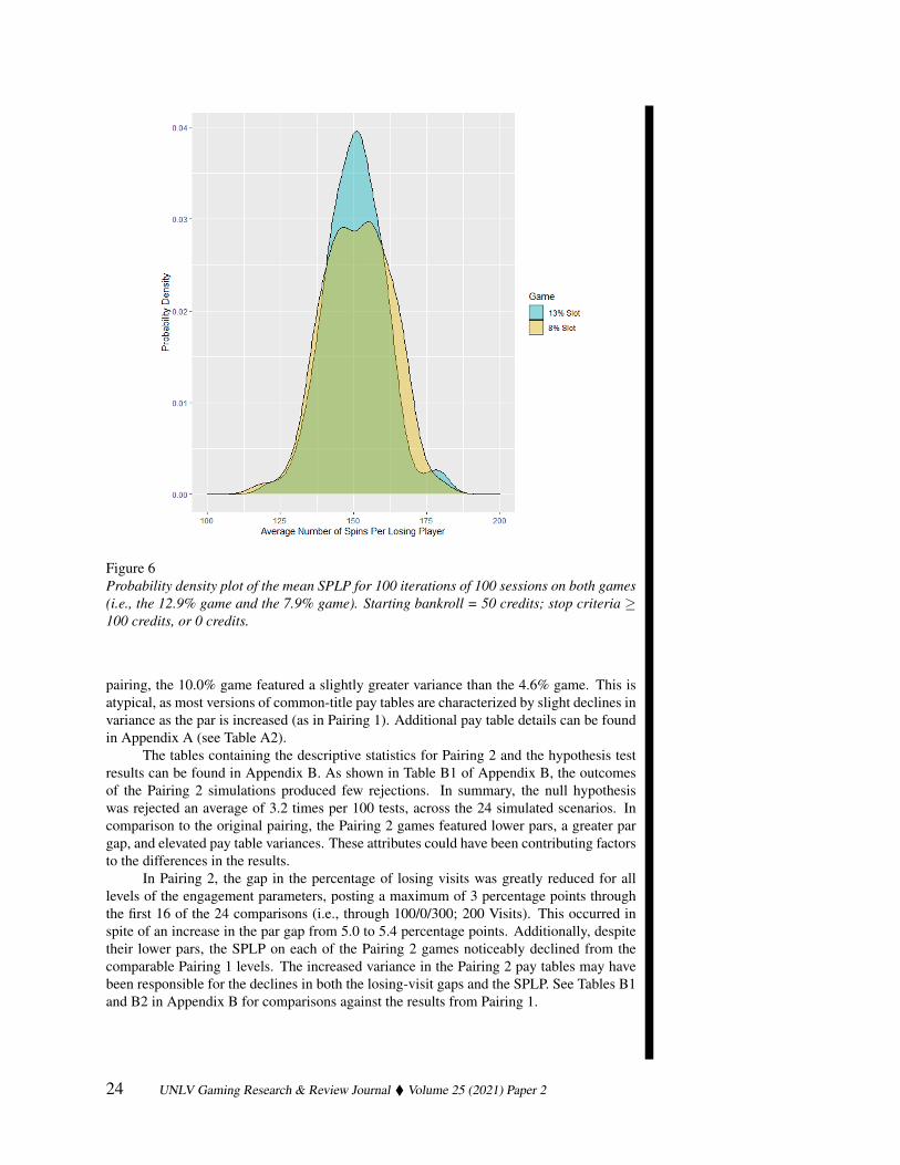
Figure 6Probability density plot of the mean SPLP for 100 iterations of 100 sessions on both games(i.e., the 12.9% game and the 7.9% game). Starting bankroll = 50 credits; stop criteria ≥100 credits, or 0 credits.

pairing, the 10.0% game featured a slightly greater variance than the 4.6% game. This isatypical, as most versions of common-title pay tables are characterized by slight declines invariance as the par is increased (as in Pairing 1). Additional pay table details can be foundin Appendix A (see Table A2).

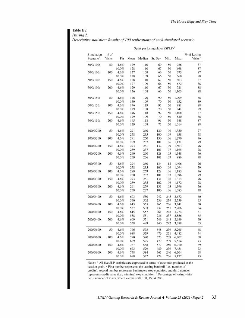
The tables containing the descriptive statistics for Pairing 2 and the hypothesis testresults can be found in Appendix B. As shown in Table B1 of Appendix B, the outcomesof the Pairing 2 simulations produced few rejections. In summary, the null hypothesiswas rejected an average of 3.2 times per 100 tests, across the 24 simulated scenarios. Incomparison to the original pairing, the Pairing 2 games featured lower pars, a greater pargap, and elevated pay table variances. These attributes could have been contributing factorsto the differences in the results.

In Pairing 2, the gap in the percentage of losing visits was greatly reduced for alllevels of the engagement parameters, posting a maximum of 3 percentage points throughthe first 16 of the 24 comparisons (i.e., through 100/0/300; 200 Visits). This occurred inspite of an increase in the par gap from 5.0 to 5.4 percentage points. Additionally, despitetheir lower pars, the SPLP on each of the Pairing 2 games noticeably declined from thecomparable Pairing 1 levels. The increased variance in the Pairing 2 pay tables may havebeen responsible for the declines in both the losing-visit gaps and the SPLP. See Tables B1and B2 in Appendix B for comparisons against the results from Pairing 1.



DiscussionGiven the overall rejection rates, the results appear to support another instance of

Tversky and Kahneman’s (1971) Law of Small Numbers. With reasonable stop criteria inplace, the samples produced by losing players generally did not allow them to produce astatistically different number of spins. This was true for Pairing 1, with its 63%-increasein par, and again for Pairing 2, which featured an increase of 117%. Even with these con-siderable increases in the pars, the individual player samples were insufficient to detect adifference in the SPLP. These results held through the 150- and 200-visit scenarios, equat-ing to 3 and 4 visits per week, respectively, for an entire year. Within the domain of losingvisits, our findings failed to support the popular view that a frequent gambler’s play timewill noticeably decline with increases in par (Frank, 2017; Gallaway, 2014; Hwang, 2019;Legato, 2015, 2019; Meczka, 2017; Wyman, 2020). As demonstrated, the idea that sam-ples from frequent gamblers are generally sufficient to identify differences in pars seemsakin to a belief in the Law of Small Numbers.

The results from Lucas and Singh (2011) were bolstered, in that they profoundlyfailed to find significant differences in the actual outcomes of play on games with differentpars, ceteris paribus. It follows that one would not expect to find a significant difference inthe number spins on paired games with similar par differences, i.e., as compared to thoseanalyzed in Lucas and Singh. The paucity of significant differences in the SPLP werein line with the game-level results from the field study research stream (Lucas & Spilde,2019a, 2019b, 2020a, 2020b). Specifically, no difference in SPLP would deter rationalplay migration to the lower-par games. It would also allow the higher-par games to subtlyaccumulate greater revenues, as consistently observed in the field studies.

The stop criteria in the simulations spotlighted the limitations of the popular heuristicregarding the relationship between par and play time, for individual gamblers. Specifically,many industry experts have contended that a 10%-increase in pars will (or must) resultin a conforming decrease in spins, ceteris paribus (Legato, 2019; Meczka, 2017; Wyman,2020).1 But individual players cannot amass enough trials for this math to bear out, and itunrealistically assumes that all players will lose their entire buy in, on each visit. Similarly,Hwang (2019) argued that lower-par games would produce noticeably different experi-ences, in terms of play time. But his premise was also based on the manifestation of along-run average within the individual gambler’s experience. He also neglected to makethe distinction between the experiences of winning and losing players.

Undoubtedly, some players will produce an outcome that reflects the game’s long-run edge, but this would be the exception to the general rule. Most reel games will producetwo groups of reasonably similar outcomes – many players who lose their entire buy in, anda few who win big. Taken together, over a sufficient number of trials, their outcomes willproduce the game’s designed advantage, i.e., its par. To the contrary, it’s very likely thatthis long-term average experience will not be representative of the single-player experience.This would be true for spins, theoretical win, and the dollar value of wagers placed (i.e.,coin-in). Similar to the argument advanced in Syed (2019), sometimes the mean describesno one. It is not always an effective measure of central tendency. This appears to be one ofthose cases.

The Real Reel ExperienceIt is difficult to imagine that actual players would be able to mentally store more than

a year’s worth of visit-level outcomes, hence the design of the current study. Plus, reel slotplayers are not likely to limit play to two games (with the same title), maintain a constant

1We offer the following empirical equation to describe their explanation of how a change in par is expected toaffect coin-in (i.e., CI) and ultimately, the number of expected spins: |%∆CI| = %∆PAR/(1+%∆PAR), wherePARGame A 6= PARGame B. Necessary assumptions include (1) Games A & B receive identical buy ins (i.e., startingbankrolls); (2) all buy-in credits are wagered until lost; (3) expected CI for each game is computed by dividingthe buy-in amount by the game’s par; and (4) a constant and equivalent wager on Games A & B. Given theseconstraints, CI becomes a proxy for the expected number of spins.


wager and buy in, strictly adhere to prescribed stop criteria, and record the number of spinsproduced on each game. Any failure to comply with these considerable engagement criteriawould only make par detection more difficult, in both the comparative and individual gameassessment conditions. This is no small point to make, as gamblers are likely to stray fromall of these critical parameters.

Given that most reel players are engaging in an entertainment-based activity, it seemsunlikely that they would adhere to such disciplined behavior, or have the awareness andknowledge to test the appropriate hypothesis, by way of the appropriate statistical method.It is fair to say, that would be asking a lot of the typical reel slot player.

The more likely scenario would entail the application of heuristics, which are crudemeasures that ignore important differences in experimental constraints. Additionally, thenature of these heuristics would surely be expected to vary across individual players. Allof this would likely occur while oscillating between titles, varying wagers and buy ins, andinterrupting play to attend to the occasional phone call or text message. Of course, thereis long list of other possible distractions and confounds. And we have not yet consideredthe presence of cognitive bias among gamblers, as observed in live gaming environments(Croson & Sundali, 2005; Sundali & Croson, 2006). Such beliefs could certainly causeplayers to stray from the experimental design. Above all, they want to win, and will likelydo whatever they believe gives them the best chance to do so.

In summary, the outcomes produced by our simulations were unaffected by the likelyundisciplined conditions of actual play. When such conditions are considered, it is difficultto conclude that actual players would be more likely to detect a difference in the number ofspins produced by the games, and ultimately, their respective pars. To the contrary, theselikely deviations from the experimental script would only impair their chances of noticinga difference. This is an important frame, as slot play does not occur in a lab.

Practical SignificanceAside from the statistical significance, there is the issue of economic/practical sig-

nificance. It is equally important to review the results from this perspective. Regarding the200-visit level of the 50/0/100 scenario in Pairing 1, Table 1 shows us that the 12.9% gameprovided 4 fewer spins than the 7.9% game (i.e., a 200-visit mean SPLP of 161 vs. 165,respectively). As for Pairing 2, the difference was 3 spins per visit, in the same scenario.Keep in mind, these mean SPLP results were computed from 100 replications of 200 an-nual visits, with play on both games. Staying with Pairing 1, it is difficult to believe that anactual player would ever notice a difference of 4 spins per visit, especially when consider-ing the aforementioned manner in which games are actually played. At 500 spins per hour,this equated to 29 seconds of play. For additional perspective, this level of visitation com-prises 4 sessions a week on each game, for 50 weeks. Such patronage would likely exceedWyman’s (2020) guidelines for frequent visitation in regional markets, i.e., “. . . upwardsof 30 to 40 visits per year.” Further, in conversations with repeater-market operators, andbased on our own experience, this would be a valuable player. Remember, this result wouldbe the same for a player with a buy in of 100 credits, and a constant 2-credit wager. Whilethe SPLP difference was negligible, there was a 5.9%-increase in the percentage of losingtrips (i.e., from 74.6% to 79.0%). But this difference also carries a standard error, so itmay not be statistically significant. The same 200-visit scenario for Pairing 2 produced nodifference in the percentage of losing trips.

In Pairing 1, the difference in the mean SPLP for the 200-visit level in the 50/0/150scenario expanded, with the 12.9% game producing 14 fewer spins per visit. This equatedto a decrease in play time of 101 seconds, assuming 500 spins per hour. But the meandifference in the proportion of losing visits declined to 3.8% (i.e., as compared to the 200-visit-level in the 50/0/100 scenario). Again, there would be an associated standard error forthis difference, diminishing the capacity of the player to detect it. In comparison, the samescenario for Pairing 2 generated a mean difference of 16 spins per visit, with losing tripsincreasing by 1.1%.



We offer these analyses of the 50-credit buy in scenarios, as we believe a bet-to-buyin ratio of 2% to be most reflective of the wagering behavior of actual reel players. Thereis some support for this assumption in Lucas and Kilby’s (2008) description of the credit-granting process for a table game player with little or no history of tracked play. Undersuch conditions the average observed wager on the player’s current trip is divided by either1.5% or 2%, to arrive at the amount of the player’s initial credit line.

Managerial ImplicationsAs others have astutely noted, the play time on reels is considerably impacted by

factors other than par (Legato, 2015; Wyman, 2020). More specifically, the amount ofplay time experienced by a gambler operating from a fixed bankroll could be materiallyimpacted by the following factors: (1) increases in pay table variance; (2) increases in therequired minimum wager and/or the cost to cover all pay lines; and (3) increases in thegame processing and reel-spin speed. Still, on balance, the industry focus seems to remainon increased pars, as the trade literature is replete with cautionary tales of its impact onthe individual gambler’s play time (Legato, 2019; Meczka, 2017; Hwang, 2019; Wyman,2020).

In Pairing 1, our aggregated results do support the admonition from industry expertsthat there will be an increase in the proportion of losing visits, as par increases (See Gall-away, 2014; Wyman, 2020). But the question remains as to whether players would notice.The differences that we observed were not substantial, and again, the ability of players tonotice them would be impeded by the previously-described battery of confounds. More-over, the bulk of results from Pairing 2 do not support the claims of noticeable increasesin the proportion of losing visits (See Table B2). Those outcomes suggest there are condi-tions that substantially limit this concern. In any case, we are not suggesting that operatorsmake drastic wholesale increases to reel slot pars. To the contrary, any changes should becarefully carried out in a stepped fashion. There are surely limits to the extent to which reelpars can be increased, without significantly affecting SPLP, the proportion of losing trips,or overall revenues.

It is our hope that this paper elucidates the shortcomings of managing “price” and/orthe “gaming value” of reel slots according the heuristic that lower pars will provide signif-icantly more play time. As demonstrated under realistic conditions there are severe limita-tions to this rule of thumb, even within the context of frequent slot play. While there maybe other conditions in which it does apply, research is needed to discover these scenarios.So far, all we have are warnings from industry experts regarding the dangers and conse-quences of increased pars. Again, there may be some, but studies are needed to specificallyidentify them.

Given the pressure to increase revenues, operators must strike a careful balance be-tween game performance and protecting the customer experience. Clearly, these two endsare closely related, but not mutually exclusive. Based on the results of this study, thefindings from Lucas and Singh (2011), and those from a host of field studies (Lucas &Spilde, 2019a, 2019b, 2020a, 2020b), there appears to be some room for improvementwith minimal exposure to risk. At some point, the popular assumption that players candetect differences in pars from play alone becomes a managerial liability. Specifically, itwill prevent operators from optimizing slot revenues.

The combination of the statistical and economic significance of our results shouldat least diminish fears of experimenting with increases in pars. Operators may be ableto make considerable gains in revenues without destroying the customer experience. Thepath to such gains is through an improved understanding of how these complex devicesproduce their outcomes. This path involves a critical evaluation of existing beliefs. Testingthe underlying assumptions expands our collective understanding of the individual player’sexperience.


Limitations & Future ResearchThe results of this simulation were limited to two modified versions of two, reel slot

titles. Still, these pay tables serve as reasonable proxies for the general math structureof many other penny reel games. Across the category, many of the base game, free-spin,and bonus structures are similar, as math constraints and market forces dictate a some-what homogenous design. Additionally, successful math is often copied with only minoralterations, resulting in a considerable level of similarity.

Of course, it is possible that certain structural differences in pay tables could producedifferent results. As correctly noted by others, there are multiple ways to manipulate pars(Lucas & Singh, 2011; Lucas & Spilde, 2020a; Wyman, 2020). Additionally, and perhapsmore importantly, some of these alterations could materially affect the pay table variance.Therefore, continued simulations such as the ones conducted here would provide valuableinsight related to the effects of specific pay table alterations on the player experience. Forexample, how would changes to the frequency of the following events affect play time:Low-end payouts, entry into free spin and bonus features, and high-end payouts? Also,expansions in the par gap beyond 5.4 percentage points may produce different results. Thisrepresents an obvious path for future research, given that the recent stream of field studyresults have found increased par gaps to produce increased gains in game-level revenues(Lucas & Spilde, 2019a, 2019b, 2020a, 2020b).

Although replicating the simulations with alternate game math would certainly pro-vide additional insight, it can be difficult to obtain and sufficiently decipher the par sheetsof licensed games. As is often the case with gaming research, gaining permission and/or ac-cess to the necessary data can be challenging. But this is understandable, as the game mathis proprietary. Given these constraints, simulations on reasonable proxies of actual gamescould be sufficiently informative regarding the effects of specific pay table components andstructures.

The results of any simulation are a function of the engagement parameters. Theoutcomes produced here challenge the idea that players would be able to detect differencesin pars under the simulated conditions. While the findings of the current study renderthe general par-play time heuristic equivocal, we cannot generalize our results beyond theassumed pay tables and the assumed player engagement conditions. For example, alteringthe ratio of the bet-per-spin to the starting bankroll could affect the results. Revisions tothe assumptions governing wagering behavior and the simulation’s start/stop criteria couldalso impact the results. While we believe our assumptions were generally reflective ofreal-world gambling behavior, much opportunity remains for further exploration.

For instance, holding the bet constant does aid in the isolation of the par effect onSPLP, but may not be reflective of actual behavior. It is far more likely that gamblers donot hold their wagers constant. Therefore, multiple levels of betting could be introducedinto future simulations to determine the impact on SPLP. This would certainly increasethe variance in any player’s outcome distribution, which would most likely make rejectionof our null hypothesis less frequent, ceteris paribus. Still, the specific impacts of variablewagering behavior on SPLP remain unknown.

Finally, it would be interesting to see what would happen if the variance in the paytable were manipulated, while holding par constant. Based on the results of Lucas andSingh (2008, 2011), significant differences in the SPLP would seem more likely. Of course,the results would depend on the magnitude of the difference in the variances.



ReferencesCroson, R. & Sundali, J. (2005). The gambler’s fallacy and the hot hand: Empirical data

from casinos. The Journal of Risk and Uncertainty, 30 (3), 195–209.Dixon, M. J., Fugelsang, J. A., MacLaren, V. V. & Harrigan, K. A. (2013). Gamblers can

discriminate ‘tight’ from ‘loose’ electronic gambling machines. InternationalGambling Studies 13, 98–111.

Gallaway, S. (2014). Killing the gaming experience. Global Gaming Business, 13 (7), 30,32.

Harrigan, K. A. & Dixon, M. (2010). Government sanctioned “tight” and “loose” slotmachines: How having multiple versions of the same slot machine game mayimpact problem gambling. Journal of Gambling Studies, 26, 159–174.

Hwang, J. (2019). When the house edge bites back. Global Gaming Business, 18 (10),24–29.

Kilby, J. & Fox, J. (1997). Casino Operations Management. New York: Wiley.Frank, B. (2017). Winning with loose slots. Global Gaming Business, 17 (5), 58–59.Legato, F. (2019). Revisiting the RTP. Global Gaming Business, 19 (6) 30–32, 34–35.Legato, F. (2015). Slot floor exodus. Global Gaming Business, 14 (4), 18–20, 22, 24.Lucas, A. F., & Kilby, J. (2008). Principles of Casino Marketing, San Diego: Gamma.Lucas, A. F., & Singh, A. K. (2008). Decreases in a slot machine’s coefficient of variation

lead to increases in customer play time. Cornell Hospitality Quarterly, 49 (2),122–133.

Lucas, A. F., & Singh, A. K. (2011). Estimating the ability of gamblers to detectdifferences in the payback percentages of reel slot machines: A closer look at theslot player experience. UNLV Gaming Research & Review Journal, 15(1), 17–36.

Lucas, A. F., Singh, A. K., & Gewali, L. (2007). Simulating the effect of pay tablestandard deviation on pulls per losing player at the single-visit level. UNLV GamingResearch & Review Journal, 11 (1), 41–52.

Lucas, A. F. & Spilde, K. A. (2019a). A deeper look into the relationship between houseadvantage and reel slot performance. Cornell Hospitality Quarterly, 60 (3),270–279.

Lucas, A. F. & Spilde, K. A. (2019b). How changes in the house advantage of reel slotsaffect game performance. Cornell Hospitality Quarterly, 60 (2), 135–149.

Lucas, A. F. & Spilde, K. A. (2020a). Examining expanded differences in slot machinepars: An analysis of revenue impacts and player sensitivity to “price.” InternationalJournal of Hospitality Management, 86. https://doi.org/10.1016/j.ijhm.2020.102450

Lucas, A. F. & Spilde, K. A. (2020b). Pushing the limits of increased casino advantage onslots: An examination of performance effects and customer reactions. CornellHospitality Quarterly. https://doi.org/10.1177%2F1938965520916436

McDonald, J. H. (2014). Handbook of Biological Statistics, 3rd ed. Baltimore, Maryland:Sparky House Publishing.

Meczka, M. (2017). Imperfect experiment: It’s wrong to say that player’s don’t noticehold differences. Global Gaming Business, 17 (5), 60.

R Core Team (2020). R: A language and environment for statistical computing. Vienna,Austria: R Foundation for Statistical Computing. Available athttps://www.R-project.org/

Singh, A. K., Lucas, A. F., Dalpatadu, R. J. & Murphy, D. J. (2013). Casino games and theCentral Limit Theorem. UNLV Gaming Research & Review Journal, 17 (2), 45–61.

Sundali, J. & Croson, R. (2006). Biases in casino betting: The hot hand and the gambler’sfallacy. Judgment and Decision Making, 1 (1), 1–12.

Syed, M. (2019). Rebel ideas: The power of diverse thinking. New York: Flatiron.Tottenham, A. (2019). Weighing in on the slots controversy. CDC Gaming Reports.

Retrieved from https://www.cdcgamingreports.com/commentaries/weighing-in-on-the-slots-controversy/


https://doi.org/10.1016/j.ijhm.2020.102450

https://doi.org/10.1177%2F1938965520916436

https://www.R-project.org/

https://www.cdcgamingreports.com/commentaries/weighing-in-on-the-slots-controversy/

https://www.cdcgamingreports.com/commentaries/weighing-in-on-the-slots-controversy/

Tversky, A. & Kahneman, D. (1971). Belief in the law of small numbers. PsychologicalBulletin,76 (2), 105–110.

Welch, B. L. (1947). The generalization of Student’s problem when several differentpopulation variances are involved. Biometrika, 34 (1–2), 28–35.

Wyman, B. (2020). Slot hold vs. slot revenue. Global Gaming Business, 19 (2), 20–23.



Appendix A

Table A1Pay table data: Pairing 1

7.9% Par (σ = 11.96) 12.9% Par (σ = 11.84)

Event p(Event) Pays p(Event) Pays

E1 0.00001017 2000 0.00001017 2000E2 0.00043741 400 0.00043741 400E3 0.00045636 200 0.00045636 200E4 0.00066446 100 0.00066446 100E5 0.00073898 75 0.00073898 45E6 0.00900695 8 0.00900695 6E7 0.00127095 7 0.00127095 4E8 0.00115095 5 0.00115095 4E9 0.00230809 4 0.00230809 3E10 0.00263227 3 0.00263227 2E11 0.00153534 2 0.00153534 2FS10 0.00476218 12 0.00476218 12FS12 0.00293704 14 0.00293704 14FS25 0.00817326 15 0.00817326 15E12 0.09257128 2 0.09257128 2E13 0.87134432 0 0.87134432 0

Table A2Pay table data: Pairing 2

4.6% Par (σ = 17.75) 10.0% Par (σ = 17.82)

Event p(Event) Pays p(Event) Pays

E1 0.00001017 4000 0.00001017 4000E2 0.00043741 500 0.00043741 500E3 0.00045436 400 0.00045436 300E4 0.00127095 12 0.00127095 10E5 0.00115095 10 0.00115095 8E6 0.00230809 6 0.00230809 6E7 0.00263227 5 0.00263227 5E8 0.00153534 3 0.00153534 3FS10 0.00476218 20 0.00476218 20FS12 0.00293704 16 0.00293704 16B1 0.00817326 15 0.00817326 15B2 0.09257128 2 0.09257128 2E13 0.88134432 0 0.88134432 0


Appendix B

Table B1Pairing 2.Summary of null hypothesis test results for losing players.SPLP: 4.6% Par vs. 10.0% Par

Buy In Sim. Stop # of Visits # of Times(in credits) Criteria to the Casino Null was

on each of 2 (in Credits) by the Player # of Times RejectedGames, on for Play on (for Play on Experiment (out ofeach Visit each Game both Games) was Repeated 100 tests)

50 0 or 100 50 100 050 0 or 100 100 100 050 0 or 100 150 100 350 0 or 100 200 100 150 0 or 150 50 100 150 0 or 150 100 100 150 0 or 150 150 100 250 0 or 150 200 100 3

100 0 or 200 50 100 1100 0 or 200 100 100 6100 0 or 200 150 100 9100 0 or 200 200 100 17100 0 or 300 50 100 0100 0 or 300 100 100 5100 0 or 300 150 100 7100 0 or 300 200 100 11200 0 or 400 50 100 0200 0 or 400 100 100 0200 0 or 400 150 100 3200 0 or 400 200 100 4200 0 or 600 50 100 0200 0 or 600 100 100 0200 0 or 600 150 100 0200 0 or 600 200 100 3



Table B2Pairing 2.Descriptive statistics: Results of 100 replications of each simulated scenario.

Spins per losing player (SPLP)1

Simulation # of % of LosingScenario2 Visits Par Mean Median St. Dev. Min. Max. Visits3

50/0/100: 50 4.6% 129 110 69 50 756 8710.0% 128 110 67 50 668 87

50/0/100: 100 4.6% 127 109 66 50 673 8710.0% 128 109 66 50 660 88

50/0/100: 150 4.6% 128 110 67 50 803 8710.0% 127 109 66 50 672 88

50/0/100: 200 4.6% 129 110 67 50 721 8810.0% 126 108 66 50 1,103 88

50/0/150: 50 4.6% 146 120 90 50 1,009 8810.0% 130 109 70 50 632 89

50/0/150: 100 4.6% 146 119 92 50 981 8810.0% 129 108 70 50 841 89

50/0/150: 150 4.6% 146 118 92 50 1,108 8710.0% 129 109 70 50 820 88

50/0/150: 200 4.6% 145 118 91 50 988 8710.0% 129 108 72 50 1,014 88

100/0/200: 50 4.6% 291 260 129 109 1,350 7710.0% 258 235 100 109 958 78

100/0/200: 100 4.6% 291 260 130 106 1,270 7610.0% 259 237 101 106 1,131 79

100/0/200: 150 4.6% 293 261 132 109 1,503 7610.0% 259 237 101 107 1,165 78

100/0/200: 200 4.6% 290 260 128 103 1,348 7610.0% 259 236 101 103 986 78

100/0/300: 50 4.6% 294 260 134 112 1,406 7610.0% 258 235 100 109 1,094 79

100/0/300: 100 4.6% 289 259 128 106 1,183 7610.0% 260 237 101 103 1,096 79

100/0/300: 150 4.6% 293 261 131 106 1,314 7610.0% 259 235 102 106 1,172 78

100/0/300: 200 4.6% 291 259 131 103 1,396 7610.0% 259 237 100 106 1,085 78

200/0/400: 50 4.6% 603 550 242 245 2,672 6010.0% 560 502 236 239 2,539 65

200/0/400: 100 4.6% 613 555 265 236 3,741 6010.0% 557 503 232 251 2,706 64

200/0/400: 150 4.6% 615 557 261 248 3,774 6110.0% 558 551 236 237 2,856 65

200/0/400: 200 4.6% 609 551 249 248 2,689 6010.0% 558 499 240 242 3,388 65

200/0/600: 50 4.6% 776 593 548 239 5,265 6810.0% 688 529 476 251 4,482 74

200/0/600: 100 4.6% 790 590 573 239 6,702 6810.0% 689 525 479 239 5,514 73

200/0/600: 150 4.6% 787 588 577 250 6,910 6910.0% 693 529 489 239 7,451 73

200/0/600: 200 4.6% 778 584 565 240 6,304 6810.0% 688 522 478 236 5,177 73

Notes: 1 All five SLP statistics are expressed in terms of outcomes produced at thesession grain. 2 First number represents the starting bankroll (i.e., number ofcredits), second number represents bankruptcy stop condition, and third numberrepresents credit value (i.e., winning) stop condition. 3 Percentage of losing visitsper n number of visits, where n equals 50, 100, 150 & 200.


The house edge and play time: Do industry heuristics ...

Documents

Transcript of The house edge and play time: Do industry heuristics ...