The HLLC Riemann Solver - Prague SumThe HLLC Approximate Riemann Solver (Toro et al, 1992). I The...

The HLLC Riemann Solver

Eleuterio TORO

Laboratory of Applied MathematicsUniversity of Trento, Italy

[email protected]

http://www.ing.unitn.it/toro

August 26, 2012

Abstract:

This lecture is about a method to solve approximatelythe Riemann problem for the Euler equations

in order to derive a numerical flux for a conservative method:

The HLLC Riemann solver

REFERENCES:

E F Toro, M Spruce and W Speares.Restoration of the contact surface in the HLL Riemann solver. Technical report CoA 9204. Department of

Aerospace Science, College of Aeronautics, Cranfield Institute of Technology. UK. June, 1992.

E F Toro, M Spruce and W Speares.Restoration of the contact surface in the Harten-Lax-van Leer Riemann solver. Shock Waves. Vol. 4, pages 25-34,

1994.

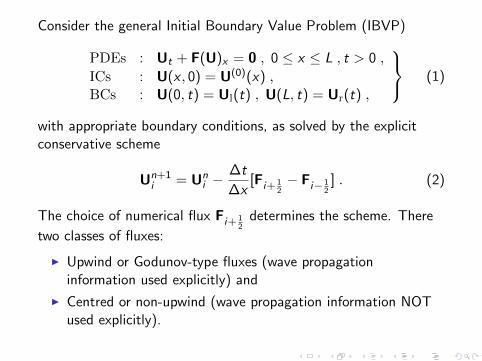
Consider the general Initial Boundary Value Problem (IBVP)

PDEs : Ut + F(U)x = 0 , 0 ≤ x ≤ L , t > 0 ,

ICs : U(x , 0) = U(0)(x) ,BCs : U(0, t) = Ul(t) , U(L, t) = Ur(t) ,

(1)

with appropriate boundary conditions, as solved by the explicitconservative scheme

Un+1i = Un

i −∆t

∆x[Fi+ 1

2− Fi− 1

2] . (2)

The choice of numerical flux Fi+ 12

determines the scheme. There

two classes of fluxes:

I Upwind or Godunov-type fluxes (wave propagationinformation used explicitly) and

I Centred or non-upwind (wave propagation information NOTused explicitly).

Godunov’s flux (Godunov 1959) is

Fi+ 12

= F(Ui+ 12(0)) , (3)

in which Ui+ 12(0) is the exact similarity solution Ui+ 1

2(x/t) of the

Riemann problem

Ut + F(U)x = 0 ,

U(x , 0) =

UL if x < 0 ,

UR if x > 0 ,

(4)

evaluated at x/t = 0.

Example: 3D Euler equations.

U =

ρρuρvρwE

, F =

ρu

ρu2 + pρuvρuw

u(E + p)

. (5)

The piece–wise constant initial data, in terms of primitivevariables, is

WL =

ρL

uL

vL

wL

pL

, WR =

ρR

uR

vR

wR

pR

. (6)

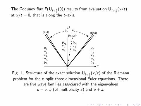
The Godunov flux F(Ui+ 12(0)) results from evaluation Ui+ 1

2(x/t)

at x/t = 0, that is along the t–axis.

*

*L *R

L R

*

ρ ρ

(u,u,u)

p u

w

LR

R

R

R

t

RR

L

L

L

L

L

ρ

(u-a) (u+a)

x0

vw

vw

ρu

pwvu

p

v

Fig. 1. Structure of the exact solution Ui+ 12(x/t) of the Riemann

problem for the x–split three dimensional Euler equations. Thereare five wave families associated with the eigenvalues

u − a, u (of multiplicity 3) and u + a.

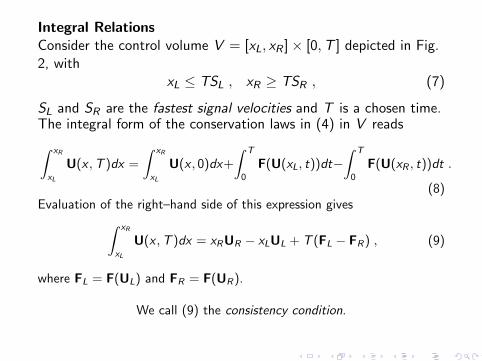
Integral RelationsConsider the control volume V = [xL, xR ]× [0,T ] depicted in Fig.2, with

xL ≤ TSL , xR ≥ TSR , (7)

SL and SR are the fastest signal velocities and T is a chosen time.The integral form of the conservation laws in (4) in V reads∫ xR

xL

U(x ,T )dx =

∫ xR

xL

U(x , 0)dx+

∫ T

0

F(U(xL, t))dt−∫ T

0

F(U(xR , t))dt .

(8)Evaluation of the right–hand side of this expression gives∫ xR

xL

U(x ,T )dx = xRUR − xLUL + T (FL − FR ) , (9)

where FL = F(UL) and FR = F(UR ).

We call (9) the consistency condition.

Now split left–hand side of (8) into three integrals, namely∫ xR

xL

U(x ,T )dx =

∫ TSL

xL

U(x ,T )dx +

∫ TSR

TSL

U(x ,T )dx +

∫ xR

TSR

U(x ,T )dx

S

xx TSTS

T

S

RL L R

L R

t

x

Fig. 2. Control volume [xL, xR ]× [0,T ] on x–t plane. SL and SR are thefastest signal velocities arising from the solution of the Riemann problem.

Evaluate the first and third terms on the right–hand side to obtain∫ xR

xL

U(x ,T )dx =

∫ TSR

TSL

U(x ,T )dx+(TSL−xL)UL+(xR−TSR)UR .

(10)Comparing (10) with (9) gives∫ TSR

TSL

U(x ,T )dx = T (SRUR − SLUL + FL − FR) . (11)

On division through by the length T (SR − SL), which is the widthof the wave system of the solution of the Riemann problembetween the slowest and fastest signals at time T , we have

1

T (SR − SL)

∫ TSR

TSL

U(x ,T )dx =SRUR − SLUL + FL − FR

SR − SL. (12)

Thus, the integral average of the exact solution of the Riemannproblem between the slowest and fastest signals at time T is aknown constant, provided that the signal speeds SL and SR areknown; such constant is the right–hand side of (12) and we denoteit by

Uhll =SRUR − SLUL + FL − FR

SR − SL. (13)

We now apply the integral form of the conservation laws to the leftportion of Fig. 10.2, that is the control volume [xL, 0]× [0,T ]. Weobtain ∫ 0

TSL

U(x ,T )dx = −TSLUL + T (FL − F0L) , (14)

where F0L is the flux F(U) along the t–axis. Solving for F0L wefind

F0L = FL − SLUL −1

T

∫ 0

TSL

U(x ,T )dx . (15)

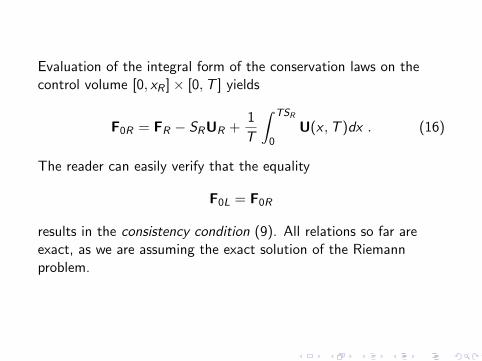
Evaluation of the integral form of the conservation laws on thecontrol volume [0, xR ]× [0,T ] yields

F0R = FR − SRUR +1

T

∫ TSR

0U(x ,T )dx . (16)

The reader can easily verify that the equality

F0L = F0R

results in the consistency condition (9). All relations so far areexact, as we are assuming the exact solution of the Riemannproblem.

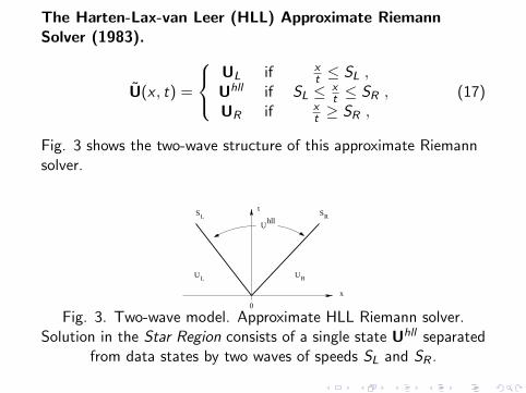
The Harten-Lax-van Leer (HLL) Approximate RiemannSolver (1983).

U(x , t) =

UL if x

t ≤ SL ,Uhll if SL ≤ x

t ≤ SR ,UR if x

t ≥ SR ,(17)

Fig. 3 shows the two-wave structure of this approximate Riemannsolver.

L SShll

R

RL UU

U

0

t

x

Fig. 3. Two-wave model. Approximate HLL Riemann solver.Solution in the Star Region consists of a single state Uhll separated

from data states by two waves of speeds SL and SR .

The HLL flux Fhll for the subsonic case SL ≤ 0 ≤ SR is found byinserting Uhll in (13) into (15) or (16) to obtain

Fhll = FL + SL(Uhll −UL) , (18)

orFhll = FR + SR(Uhll −UR) . (19)

Use of (13) in (18) or (19) gives the HLL flux

Fhll =SRFL − SLFR + SLSR(UR −UL)

SR − SL(20)

for the subsonic case SL ≤ 0 ≤ SR .

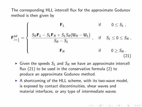
The corresponding HLL intercell flux for the approximate Godunovmethod is then given by

Fhlli+ 1

2=

FL if 0 ≤ SL ,

SRFL − SLFR + SLSR(UR −UL)

SR − SL, if SL ≤ 0 ≤ SR ,

FR if 0 ≥ SR .(21)

I Given the speeds SL and SR we have an approximate intercellflux (21) to be used in the conservative formula (2) toproduce an approximate Godunov method.

I A shortcoming of the HLL scheme, with its two-wave model,is exposed by contact discontinuities, shear waves andmaterial interfaces, or any type of intermediate waves.

The HLLC Approximate Riemann Solver (Toro et al, 1992).

I The HLLC scheme is a modification of the HLL schemewhereby the missing contact and shear waves in the Eulerequations are restored.

I HLLC for the Euler equations has a three-wave model

S

RL UU

*

RL ** UU

RL SS

0

t

x

Fig. 4. HLLC approximate Riemann solver. Solution in the StarRegion consists of two constant states separated from each other

by a middle wave of speed S∗.

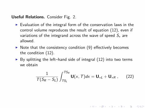
Useful Relations. Consider Fig. 2.

I Evaluation of the integral form of the conservation laws in thecontrol volume reproduces the result of equation (12), even ifvariations of the integrand across the wave of speed S∗ areallowed.

I Note that the consistency condition (9) effectively becomesthe condition (12).

I By splitting the left–hand side of integral (12) into two termswe obtain

1

T (SR − SL)

∫ TSR

TSL

U(x ,T )dx = U∗L + U∗R , (22)

where the following integral averages are introduced

U∗L =1

T (S∗ − SL)

∫ TS∗

TSL

U(x ,T )dx ,

U∗R =1

T (SR − S∗)

∫ TSR

TS∗

U(x ,T )dx .

(23)

Use of (23) into (22) and use of (12), make condition (9)(S∗ − SL

SR − SL

)U∗L +

(SR − S∗SR − SL

)U∗R = Uhll , (24)

The HLLC approximate Riemann solver is given as follows

U(x , t) =

UL , if x

t ≤ SL ,U∗L , if SL ≤ x

t ≤ S∗ ,U∗R , if S∗ ≤ x

t ≤ SR ,UR , if x

t ≥ SR .

(25)

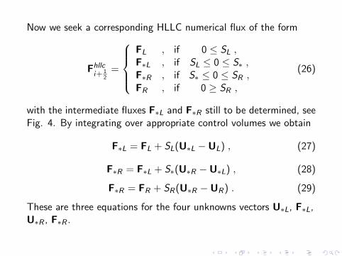
Now we seek a corresponding HLLC numerical flux of the form

Fhllci+ 1

2=

FL , if 0 ≤ SL ,F∗L , if SL ≤ 0 ≤ S∗ ,F∗R , if S∗ ≤ 0 ≤ SR ,FR , if 0 ≥ SR ,

(26)

with the intermediate fluxes F∗L and F∗R still to be determined, seeFig. 4. By integrating over appropriate control volumes we obtain

F∗L = FL + SL(U∗L −UL) , (27)

F∗R = F∗L + S∗(U∗R −U∗L) , (28)

F∗R = FR + SR(U∗R −UR) . (29)

These are three equations for the four unknowns vectors U∗L, F∗L,U∗R , F∗R .

We seek the solution for the two unknown intermediate fluxes F∗L

and F∗R . There are more unknowns than equations and some extraconditions need to be imposed, in order to solve the algebraicproblem. We impose

p∗L = p∗R = p∗ ,u∗L = u∗R = u∗ ,

}for pressure and normal velocity (30)

v∗L = vL , v∗R = vR ,w∗L = wL , w∗R = wR .

}for tangential velocities

(31)Conditions (30), (31) are identically satisfied by the exact solution.In addition we impose

S∗ = u∗ (32)

and thus if an estimate for S∗ is known, the normal velocitycomponent u∗ in the Star Region is known.

Now equations (27) and (29) can be re–arranged as

SLU∗L − F∗L = SLUL − FL , (33)

SRU∗R − F∗R = SRUR − FR , (34)

where the right–hand sides of (33) and (34) are known constantvectors (data). We also note the useful relation

F(U) = uU + pD , D = [0, 1, 0, 0, u]T . (35)

Assuming SL and SR to be known and performing algebraicmanipulations of the first and second components of equations(33)–(34) one obtains

p∗L = pL+ρL(SL−uL)(S∗−uL) , p∗R = pR +ρR(SR−uR)(S∗−uR) .(36)

From (30) p∗L = p∗R , which from (36) gives

S∗ =pR − pL + ρLuL(SL − uL)− ρRuR(SR − uR)

ρL(SL − uL)− ρR(SR − uR). (37)

Manipulation of (33) and (34) and using p∗L and p∗R from (36)gives

F∗K = FK + SK (U∗K −UK ) , (38)

for K=L and K=R, with the intermediate states given as

U∗K = ρK

(SK − uK

SK − S∗

)

1S∗vK

wK

EK

ρK+ (S∗ − uK )

[S∗ +

pK

ρK (SK − uK )

]

.

(39)The final choice of the HLLC flux is made according to (26).

Variation 1 of HLLC.From equations (33) and (34) we may write the following solutionsfor the state vectors U∗L and U∗R

U∗K =SK UK − FK + p∗K D∗

SL − S∗, D∗ = [0, 1, 0, 0,S∗] , (40)

with p∗L and p∗R as given by (36). Substitution of p∗K from (36)into (40) followed by use of (27) and (29) gives direct expressionsfor the intermediate fluxes as

F∗K =S∗(SK UK − FK ) + SK (pK + ρL(SK − uK )(S∗ − uK ))D∗

SK − S∗,

(41)with the final choice of the HLLC flux made again according to(26).

Variation 2 of HLLC.A different HLLC flux is obtained by assuming a single meanpressure value in the Star Region, and given by the arithmeticaverage of the pressures in (36), namely

PLR =1

2[pL + pR +ρL(SL−uL)(S∗−uL) +ρR(SR −uR)(S∗−uR)] .

(42)Then the intermediate state vectors are given by

U∗K =SK UK − FK + PLRD∗

SK − S∗. (43)

Substitution of these into (27) and (29) gives the fluxes F∗L andF∗R as

F∗K =S∗(SK UK − FK ) + SK PLRD∗

SK − S∗. (44)

Again the final choice of HLLC flux is made according to (26).

Remarks.

I The original HLLC formulation (38)–(39) enforces thecondition p∗L = p∗R , which is satisfied by the exact solution.

I In the alternative HLLC formulation (41) we relax suchcondition, being more consistent with the pressureapproximations (36).

I There is limited practical experience with the alternativeHLLC formulations (41) and (44).

I General equation of state. All manipulations, assuming thatwave speed estimates for SL and SR are available, are valid forany equation of state; this only enters when prescribingestimates for SL and SR .

Multidimensional multicomponent flow.Consider the advection of a chemical species of concentrations ql

by the normal flow speed u. Then we can write the followingadvection equation

∂tql + u∂x ql = 0 , for l = 1, . . . ,m .

Note that these equations are written in non–conservative form.However, by combining these with the continuity equation weobtain a conservative form of these equations, namely

(ρql )t + (ρuql )x = 0 , for l = 1, . . . ,m .

The eigenvalues of the enlarged system are as before, with theexception of λ2 = u, which now, in three space dimensions, hasmultiplicity m + 3.

These conservation equations can then be added as newcomponents to the conservation equations in (1) or (4), with theenlarged vectors of conserved variables and fluxes given as

U =

ρρuρvρwEρq1

. . .ρql

. . .ρqm

, F =

ρuρu2 + pρuvρuw

u(E + p)ρuq1

. . .ρuql

. . .ρuqm

. (45)

The HLLC flux accommodates these new equations in a verynatural way, and nothing special needs to be done. If the HLLCflux (38) is used, with F as in (45), then the intermediate statevectors are given by

U∗K = ρK

(SK − uK

SK − S∗

)

1S∗vK

wK

EK

ρK+ (S∗ − uK )

[S∗ +

pK

ρK (SK − uK )

](q1)K

. . .(ql )K

. . .(qm)K

.

(46)for K = L and K = R.

Wave Speed Estimates

We need estimates SL, S∗ and SR . Davis (1988) suggested

SL = uL − aL , SR = uR + aR , (47)

SL = min {uL − aL, uR − aR} , SR = max {uL + aL, uR + aR} .(48)

Both Davis (1988) and Einfeldt (1988), proposed

SL = u − a , SR = u + a , (49)

u and a are the Roe–average particle and sound speeds respectively

u =

√ρLuL +

√ρRuR√

ρL +√ρR

, a =

[(γ − 1)(H − 1

2u2)

]1/2

, (50)

with the enthalpy H = (E + p)/ρ approximated as

H =

√ρLHL +

√ρRHR√

ρL +√ρR

. (51)

Einfeldt (1988) proposed the estimates

SL = u − d , SR = u + d , (52)

for his HLLE solver, where

d2 =

√ρLa2

L +√ρRa2

R√ρL +

√ρR

+ η2(uR − uL)2 (53)

and

η2 =1

2

√ρL√ρR

(√ρL +

√ρR)2

. (54)

These wave speed estimates are reported to lead to effective androbust Godunov–type schemes.

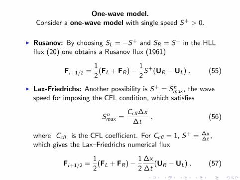
One-wave model.Consider a one-wave model with single speed S+ > 0.

I Rusanov: By choosing SL = −S+ and SR = S+ in the HLLflux (20) one obtains a Rusanov flux (1961)

Fi+1/2 =1

2(FL + FR)− 1

2S+(UR −UL) . (55)

I Lax-Friedrichs: Another possibility is S+ = Snmax , the wave

speed for imposing the CFL condition, which satisfies

Snmax =

Ccfl ∆x

∆t, (56)

where Ccfl is the CFL coefficient. For Ccfl = 1, S+ = ∆x∆t ,

which gives the Lax–Friedrichs numerical flux

Fi+1/2 =1

2(FL + FR)− 1

2

∆x

∆t(UR −UL) . (57)

Pressure–Based Wave Speed Estimates

Toro et al. (1994) suggested to first find an estimate p∗ for thepressure in the Star Region and then take

SL = uL − aLqL , SR = uR + aRqR , (58)

qK =

1 if p∗ ≤ pK[

1 +γ + 1

2γ(p∗/pK − 1)

]1/2

if p∗ > pK .(59)

I This choice discriminates between shocks and rarefactions.

I If the K wave is a rarefaction then the speed SK is the speedof the head of the rarefaction, the fastest signal.

I If the K wave is a shock wave then the speed is anapproximation of the shock speed.

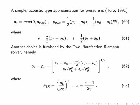
A simple, acoustic type approximation for pressure is (Toro, 1991)

p∗ = max(0, ppvrs) , ppvrs =1

2(pL + pR)− 1

2(uR − uL)ρa , (60)

where

ρ =1

2(ρL + ρR) , a =

1

2(aL + aR) . (61)

Another choice is furnished by the Two–Rarefaction Riemannsolver, namely

p∗ = ptr =

[aL + aR − γ−1

2 (uR − uL)

aL/pzL + aR/pz

R

]1/z

, (62)

where

PLR =

(pL

pR

)z

; z =γ − 1

2γ. (63)

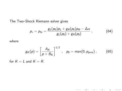
The Two–Shock Riemann solver gives

p∗ = pts =gL(p0)pL + gR(p0)pR −∆u

gL(p0) + gR(p0), (64)

where

gK (p) =

[AK

p + BK

]1/2

, p0 = max(0, ppvrs) , (65)

for K = L and K = R.

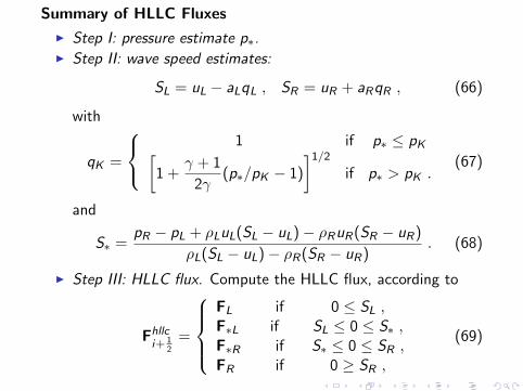
Summary of HLLC Fluxes

I Step I: pressure estimate p∗.I Step II: wave speed estimates:

SL = uL − aLqL , SR = uR + aRqR , (66)

with

qK =

1 if p∗ ≤ pK[

1 +γ + 1

2γ(p∗/pK − 1)

]1/2

if p∗ > pK .(67)

and

S∗ =pR − pL + ρLuL(SL − uL)− ρRuR(SR − uR)

ρL(SL − uL)− ρR(SR − uR). (68)

I Step III: HLLC flux. Compute the HLLC flux, according to

Fhllci+ 1

2=

FL if 0 ≤ SL ,F∗L if SL ≤ 0 ≤ S∗ ,F∗R if S∗ ≤ 0 ≤ SR ,FR if 0 ≥ SR ,

(69)

F∗K = FK + SK (U∗K −UK ) (70)

and

U∗K = ρK

(SK − uK

SK − S∗

)

1S∗vK

wK

EK

ρK+ (S∗ − uK )

[S∗ +

pK

ρK (SK − uK )

]

.

(71)

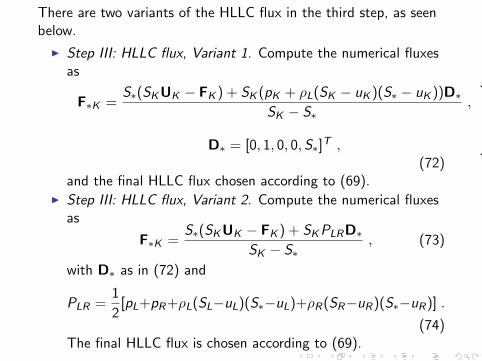
There are two variants of the HLLC flux in the third step, as seenbelow.

I Step III: HLLC flux, Variant 1. Compute the numerical fluxesas

F∗K =S∗(SK UK − FK ) + SK (pK + ρL(SK − uK )(S∗ − uK ))D∗

SK − S∗,

D∗ = [0, 1, 0, 0,S∗]T ,

(72)

and the final HLLC flux chosen according to (69).I Step III: HLLC flux, Variant 2. Compute the numerical fluxes

as

F∗K =S∗(SK UK − FK ) + SK PLRD∗

SK − S∗, (73)

with D∗ as in (72) and

PLR =1

2[pL+pR +ρL(SL−uL)(S∗−uL)+ρR(SR−uR)(S∗−uR)] .

(74)The final HLLC flux is chosen according to (69).

Numerical Results

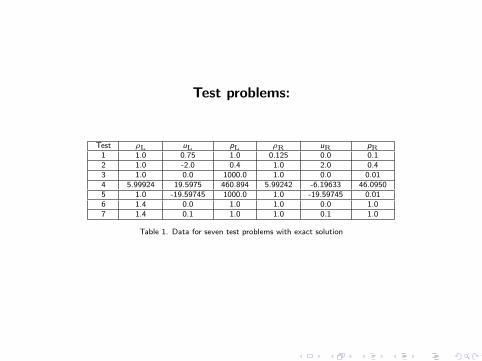
Test problems:

Test ρL uL pL ρR uR pR1 1.0 0.75 1.0 0.125 0.0 0.12 1.0 -2.0 0.4 1.0 2.0 0.43 1.0 0.0 1000.0 1.0 0.0 0.014 5.99924 19.5975 460.894 5.99242 -6.19633 46.09505 1.0 -19.59745 1000.0 1.0 -19.59745 0.016 1.4 0.0 1.0 1.0 0.0 1.07 1.4 0.1 1.0 1.0 0.1 1.0

Table 1. Data for seven test problems with exact solution

0

0.5

1

0 0.5 1

Den

sity

Position

0

0.8

1.6

0 0.5 1

Vel

ocity

Position

0

0.5

1

0 0.5 1

Pres

sure

Position

1.8

3.8

0 0.5 1

Inte

rnal

ene

rgy

Position

Godunov’s method with HLLC Riemann solver applied to Test 1,with x0 = 0.3. Numerical (symbol) and exact (line) solutions are

compared at time 0.2.

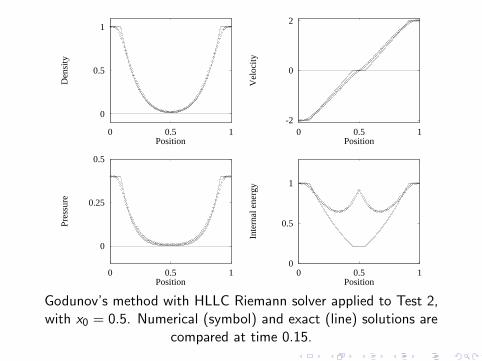
0

0.5

1

0 0.5 1

Den

sity

Position

-2

0

2

0 0.5 1

Vel

ocity

Position

0

0.25

0.5

0 0.5 1

Pres

sure

Position

0

0.5

1

0 0.5 1

Inte

rnal

ene

rgy

Position



0

3

6

0 0.5 1

Den

sity

Position

0

12.5

25

0 0.5 1

Vel

ocity

Position

0

500

1000

0 0.5 1

Pres

sure

Position

0

1250

2500

0 0.5 1

Inte

rnal

ene

rgy

Position



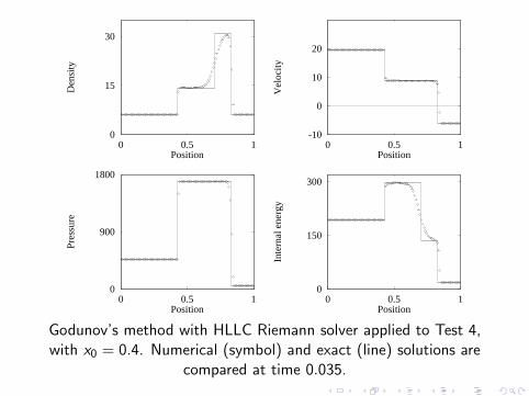
0

15

30

0 0.5 1

Den

sity

Position

-10

0

10

20

0 0.5 1

Vel

ocity

Position

0

900

1800

0 0.5 1

Pres

sure

Position

0

150

300

0 0.5 1

Inte

rnal

ene

rgy

Position



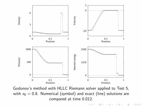
0

3

6

0 0.5 1

Den

sity

Position

-20

0

5

0 0.5 1

Vel

ocity

Position

0

500

1000

0 0.5 1

Pres

sure

Position

0

1250

2500

0 0.5 1

Inte

rnal

ene

rgy

Position



0

3

6

0 0.5 1

Den

sity

Position

-20

0

5

0 0.5 1

Vel

ocity

Position

0

500

1000

0 0.5 1

Pres

sure

Position

0

1250

2500

0 0.5 1

Inte

rnal

ene

rgy

Position

Godunov’s method with HLL Riemann solver applied to Test 5,with x0 = 0.8. Numerical (symbol) and exact (line) solutions are


1

1.4

0 0.5 1

HL

L d

ensi

ty

position

1

1.4

0 0.5 1

HL

LC

den

sity

position

1

1.4

0 0.5 1

HL

L d

ensi

ty

position

1

1.4

0 0.5 1

HL

LC

den

sity

position

Godunov’s method with HLL (left) and HLLC (right) Riemannsolvers applied to Tests 6 and 7. Numerical (symbol) and exact

(line) solutions are compared at time 2.0.

Closing Remarks:

I We have presented HLLC for the Euler equations.

I For the 2D shallow water equations see Toro E F Shockcapturing methods for free-surface shallow flows. Wiley andSons, 2001.

I For Turbulent flow applications (implicit version of HLLC), seeBatten, Leschziner and Goldberg (1997).

I For extensions to MHD equations see Gurski (2004), Li(2005), Mignone et al. (2006++).

I For application to two-phase flow see Tokareva and Toro, JCP(2010).

I For extensions see Takahiro (2005) and Bouchut (2007),Mignone (2005).

The HLLC Riemann Solver - Prague SumThe HLLC Approximate Riemann Solver (Toro et al, 1992). I The...

Documents

Transcript of The HLLC Riemann Solver - Prague SumThe HLLC Approximate Riemann Solver (Toro et al, 1992). I The...