USGSscience for a changing world

The History of Stream Gaging in Ohio

Introduction

Streams are a natural resource that can influence economic growth and the development of communities. They sup­ ply water for many uses, provide habitat for aquatic plants and animals, and sup­ port recreational activities such as boat­ ing and fishing. The amount of water (flow) in a stream either too little or too much can seriously affect these uses and human life. By using a method called stream gaging, information about the flow in a stream and the fluctuations in that flow can be obtained.

In its simplest form, stream gaging may consist of measuring any number of the following stream characteristics: stage (or depth), cross-sectional area, velocity, and (or) flow (or discharge). When the depth and velocity are mea­ sured at several points across the stream channel so that the flow (or discharge) is calculated, a streamflow measurement (or discharge measurement) is made (historical example shown in fig. 1).

By making streamflow measure­ ments at the same site on a stream over a wide range of stages, a relation between stage and discharge can be developed. This relation can be used to provide information on the magnitude and fluctu­ ations of flow on a stream. If long-term or continuous information is needed on a specific site, a stream-gaging station can be established. A stream-gaging sta­ tion is a site where stage is monitored and recorded and streamflow measure­ ments are made to provide a stage-dis­ charge relation.

Ever since the first documented streamflow measurement was made in Ohio on the Sandusky River stream-gaging information has been used to minimize the effects of floods and droughts, determine locations for water intakes and wastewater-treatment plants,

and provide data for many other uses. Today,stream gaging is a routine activity in managing the State's water resources.

Early stream gaging

Before 1921, when the first stations in Ohio's present-day stream-gaging net­ work were established, streams were monitored not only by government agen­ cies but also by pri­ vate institutions. Early stream gaging was done irregularly and the quality and accuracy of the data varied. Often, the stream-gaging infor­ mation was lost because it went unpublished.

The first docu­ mented streamflow measurement in Ohio was made in August 1823 on the Sandusky River and was pub­ lished by the Canal Commission. This measurement, along with more than 40 other measurements before 1825, was used to determine whether the central Ohio area had enou; h flow during dry peri­ ods to support a canal system (Frost, 1987).

Later, around the time of the Civil War, more than 1,000 mills in Ohio used stream- flow as their power source. Because the mill operators were

concerned about the dependability of this power source, they would make stream- flow measurements. Like many other streamflow measurements made during this time, these measurements were never published and were eventually lost.

After 1858 , the U.S. Weather Bureau worked with observers to read and docu­ ment river stages from staff gages and

Figure 1. Stream gager making a streamflow measurement using a bridge crane and a current meter. Picture taken in the 1940's from a bridge near The Ohio State University (OSU). OSU worked with the USGS to build a stream-gaging- station network in Ohio.

U.S. Department of the Interior U.S. Geological Survey

USGS Fact Sheet 050-00 May 2000

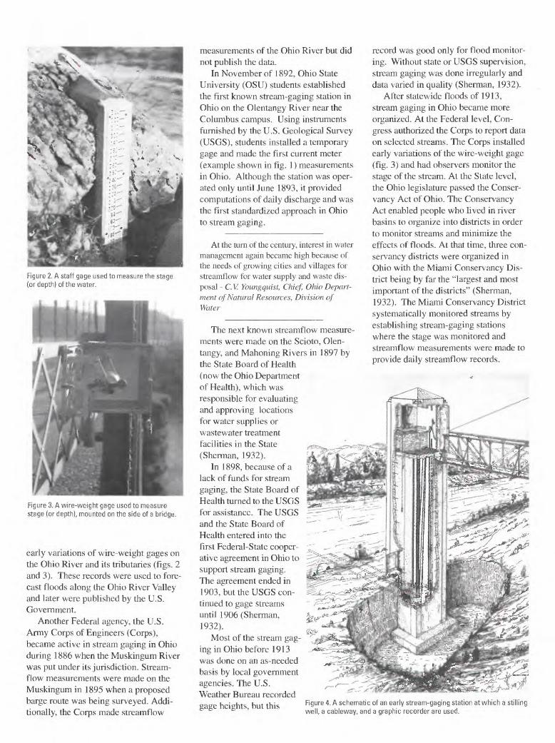
Figure 2. A staff gage used to measure the stage (or depth) of the water.

Figure 3. A wire-weight gage used to measure stage (or depth), mounted on the side of a bridge.

early variations of wire-weight gages on the Ohio River and its tributaries (figs. 2 and 3). These records were used to fore­ cast floods along the Ohio River Valley and later were published by the U.S. Government.

Another Federal agency, the U.S. Army Corps of Engineers (Corps), became active in stream gaging in Ohio during 1886 when the Muskingum River was put under its jurisdiction. Stream- flow measurements were made on the Muskingum in 1895 when a proposed barge route was being surveyed. Addi­ tionally, the Corps made streamflow

measurements of the Ohio River but did not publish the data.

In November of 1892, Ohio State University (OSU) students established the first known stream-gaging station in Ohio on the Olentangy River near the Columbus campus. Using instruments furnished by the U.S. Geological Survey (USGS), students installed a temporary gage and made the first current meter (example shown in fig. 1) measurements in Ohio. Although the station was oper­ ated only until June 1893, it provided computations of daily discharge and was the first standardized approach in Ohio to stream gaging.

At the turn of the century, interest in water management again became high because of the needs of growing cities and villages for streamflow for water supply and waste dis­ posal - C.V. Youngquist, Chief, Ohio Depart­ ment of Natural Resources, Division of Water

The next known streamflow measure­ ments were made on the Scioto, Olen­ tangy, and Mahoning Rivers in 1897 by the State Board of Health (now the Ohio Department of Health), which was responsible for evaluating and approving locations for water supplies or wastewater treatment facilities in the State (Sherman, 1932).

In 1898, because of a lack of funds for stream gaging, the State Board of Health turned to the USGS for assistance. The USGS and the State Board of Health entered into the first Federal-State cooper­ ative agreement in Ohio to support stream gaging. The agreement ended in 1903, but the USGS con­ tinued to gage streams until 1906 (Sherman, 1932).

Most of the stream gag­ ing in Ohio before 1913 was done on an as-needed basis by local government agencies. The U.S. Weather Bureau recorded gage heights, but this

record was good only for flood monitor­ ing. Without state or USGS supervision, stream gaging was done irregularly and data varied in quality (Sherman, 1932).

After statewide floods of 1913, stream gaging in Ohio became more organized. At the Federal level, Con­ gress authorized the Corps to report data on selected streams. The Corps installed early variations of the wire-weight gage (fig. 3) and had observers monitor the stage of the stream. At the State level, the Ohio legislature passed the Conser­ vancy Act of Ohio. The Conservancy Act enabled people who lived in river basins to organize into districts in order to monitor streams and minimize the effects of floods. At that time, three con­ servancy districts were organized in Ohio with the Miami Conservancy Dis­ trict being by far the "largest and most important of the districts" (Sherman, 1932). The Miami Conservancy District systematically monitored streams by establishing stream-gaging stations where the stage was monitored and streamflow measurements were made to provide daily streamflow records.

7Figure 4. A schematic of an early stream-gaging station at which a stilling well, a cableway, and a graphic recorder are used.

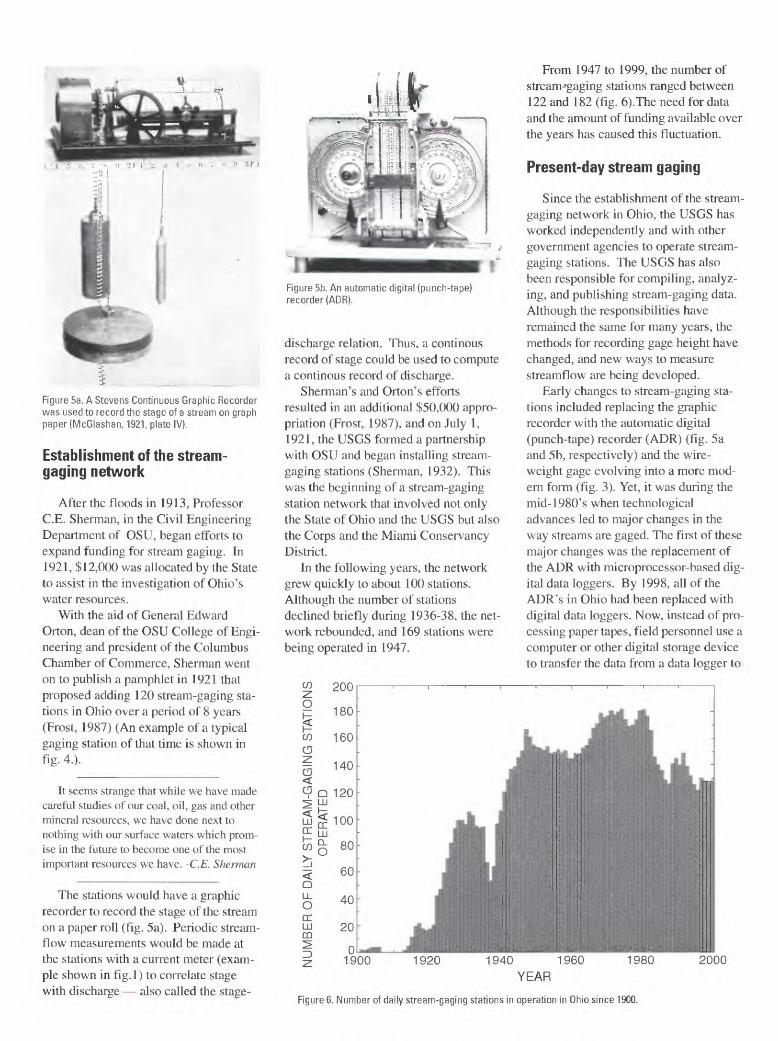
Figure 5a. A Stevens Continuous Graphic Recorder was used to record the stage of a stream on graph paper (McGlashan, 1921, plate IV).

Establishment of the stream- gaging network

After the floods in 1913, Professor C.E. Sherman, in the Civil Engineering Department of OSU, began efforts to expand funding for stream gaging. In 1921, $ 12,000 was allocated by the State to assist in the investigation of Ohio's water resources.

With the aid of General Edward Orton, dean of the OSU College of Engi­ neering and president of the Columbus Chamber of Commerce, Sherman went on to publish a pamphlet in 1921 that proposed adding 120 stream-gaging sta­ tions in Ohio over a period of 8 years (Frost, 1987) (An example of a typical gaging station of that time is shown in fig- 4.).

It seems strange that while we have made careful studies of our coal, oil, gas and other mineral resources, we have done next to nothing with our surface waters which prom­ ise in the future to become one of the most important resources we have. -C.E. Sherman

The stations would have a graphic recorder to record the stage of the stream on a paper roll (fig. 5a). Periodic stream- flow measurements would be made at the stations with a current meter (exam­ ple shown in fig. 1) to correlate stage with discharge also called the stage-

Figure 5b. An automatic digital (punch-tape) recorder (ADR).

discharge relation. Thus, a continous record of stage could be used to compute a continous record of discharge.

Sherman's and Orton's efforts resulted in an additional $50,000 appro­ priation (Frost, 1987), and on July 1, 1921, the USGS formed a partnership with OSU and began installing stream- gaging stations (Sherman, 1932). This was the beginning of a stream-gaging station network that involved not only the State of Ohio and the USGS but also the Corps and the Miami Conservancy District.

In the following years, the network grew quickly to about 100 stations. Although the number of stations declined briefly during 1936-38, the net­ work rebounded, and 169 stations were being operated in 1947.

From 1947 to 1999, the number of streanvgaging stations ranged between 122 and 182 (fig. 6).The need for data and the amount of funding available over the years has caused this fluctuation.

Present-day stream gaging

Since the establishment of the stream- gaging network in Ohio, the USGS has worked independently and with other government agencies to operate stream- gaging stations. The USGS has also been responsible for compiling, analyz­ ing, and publishing stream-gaging data. Although the responsibilities have remained the same for many years, the methods for recording gage height have changed, and new ways to measure streamflow are being developed.

Early changes to stream-gaging sta­ tions included replacing the graphic recorder with the automatic digital (punch-tape) recorder (ADR) (fig. 5a and 5b, respectively) and the wire- weight gage evolving into a more mod­ ern form (fig. 3). Yet, it was during the mid-1980's when technological advances led to major changes in the way streams are gaged. The first of these major changes was the replacement of the ADR with microprocessor-based dig­ ital data loggers. By 1998, all of the ADR's in Ohio had been replaced with digital data loggers. Now, instead of pro­ cessing paper tapes, field personnel use a computer or other digital storage device to transfer the data from a data logger to

1920 1W4U 19bU

YEAR

1980 2000

Figure 6. Number of daily stream-gaging stations in operation in Ohio since 1900.

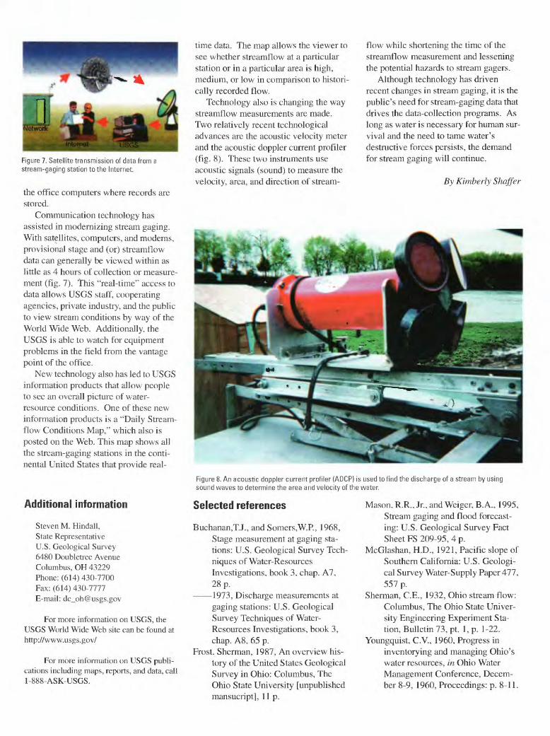
Figure 7. Satellite transmission of data from a stream-gaging station to the Internet.

the office computers where records are stored.

Communication technology has assisted in modernizing stream gaging. With satellites, computers, and modems, provisional stage and (or) streamflow data can generally be viewed within as little as 4 hours of collection or measure­ ment (fig. 7). This "real-time'" access to data allows USGS staff, cooperating agencies, private industry, and the public to view stream conditions by way of the World Wide Web. Additionally, the USGS is able to watch for equipment problems in the field from the vantage point of the office.

New technology also has led to USGS information products that allow people to see an overall picture of water- resource conditions. One of these new information products is a "Daily Stream- flow Conditions Map," which also is posted on the Web. This map shows all the stream-gaging stations in the conti­ nental United States that provide real-

Additional information

Steven M. Hindall, State Representative U.S. Geological Survey 6480 Doubletree Avenue Columbus, OH 43229 Phone:(614)430-7700 Fax:(614)430-7777 E-mail: dc_oh@usgs.gov

For more information on USGS, the USGS World Wide Web site can be found at http://www.usgs.gov/

For more information on USGS publi­ cations including maps, reports, and data, call 1-888-ASK-USGS.

time data. The map allows the viewer to see whether streamflow at a particular station or in a particular area is high, medium, or low in comparison to histori­ cally recorded flow.

Technology also is changing the way streamflow measurements are made. Two relatively recent technological advances are the acoustic velocity meter and the acoustic doppler current profiler (fig. 8). These two instruments use acoustic signals (sound) to measure the velocity, area, and direction of stream-

flow while shortening the time of the streamflow measurement and lessening the potential hazards to stream gagers.

Although technology has driven recent changes in stream gaging, it is the public's need for stream-gaging data that drives the data-collection programs. As long as water is necessary for human sur­ vival and the need to tame water's destructive forces persists, the demand for stream gaging will continue.

By Kimberly Shaffer

Figure 8. An acoustic doppler current profiler (ADCP) is used to find the discharge of a stream by using sound waves to determine the area and velocity of the water.

Selected references

Buchanan,T.J., and Somers,W.R, 1968, Stage measurement at gaging sta­ tions: U.S. Geological Survey Tech­ niques of Water-Resources Investigations, book 3, chap. A7, 28 p.

1973, Discharge measurements at gaging stations: U.S. Geological Survey Techniques of Water- Resources Investigations, book 3, chap. A8, 65 p.

Frost. Sherman, 1987, An overview his­ tory of the United States Geological Survey in Ohio: Columbus, The Ohio State University [unpublished mansucript], lip.

Mason, R.R., Jr., and Weiger, B.A., 1995, Stream gaging and flood forecast­ ing: U.S. Geological Survey Fact Sheet FS 209-95, 4 p.

McGlashan, H.D., 1921, Pacific slope of Southern California: U.S. Geologi­ cal Survey Water-Supply Paper 477, 557 p.

Sherman, C.E., 1932, Ohio stream flow: Columbus, The Ohio State Univer­ sity Engineering Experiment Sta­ tion, Bulletin 73, pt. 1, p. 1-22.

Youngquist, C.V., 1960, Progress in inventorying and managing Ohio's water resources, in Ohio Water Management Conference, Decem­ ber 8-9, 1960, Proceedings: p. 8-11.