THE HF RESISTANCE OF SINGLE LAYER COILS -...

Payne : The HF Resistance of Single Layer Coils

1

THE HF RESISTANCE OF SINGLE LAYER COILS

The problem of finding the alternating-current resistance of single layer coils has been

analysed by Butterworth, in a series of very complicated papers. It is shown here that by

taking a different approach the analysis is relatively easy and produces simple equations

which agree very well with published experimental measurements.

The analysis presented here includes coils wound with flat conducting tape as well as

conductors of circular cross-section.

1. INTRODUCTION

The alternating current resistance of single layer coils wound with round wire presents serious

mathematical difficulties but was attempted by Butterworth in the 1920’s in a series of complicated papers,

and summarised by Terman (ref 1). However his analysis has been shown to be not very accurate for the

important case of close wound coils (Medhurst ref 2). In 1951 a more accurate theory was developed by

Arnold (ref 3), but again the analysis is complicated and the resulting equations difficult to use.

One reason for the complication is the difficulty in calculating the strength of the magnetic fields which

intercept the conductor, since it is these which determine the loss. The analysis here takes a totally different

approach to the problem by deriving these fields from Nagaoka’s factor, normally used in the calculation of

the inductance.

The analysis here is for solid conductors only (not stranded) and for frequencies high enough that the skin

depth is a small fraction of the wire diameter, or a small fraction of the strip thickness if wound with thin

strip. In practice this is often not possible with round wire and then the effective diameter of the wire must

be used (see Section 6).

In the following text key equations are highlighted in red.

2. PREVIOUS WORK

2.1. Previous Theoretical Work

It is well known that the resistance of isolated conductors at high frequency is much larger than the dc

resistance and this is due to the skin effect, so-called because at sufficiently high frequencies the current

penetrates into the conductor only a small amount, and flows in only a thin skin down the outside of the

conductor.

Skin effect arises because of the magnetic field which the conductor produces around itself, but if this field

also intercepts other conductors this will also increase its resistance. In particular if the wire is wound into a

coil, each turn of the wire induces loss-making eddy currents into adjacent turns, indeed even of turns some

distance away in that it contributes to an overall field down the coil. The power lost in these eddy currents

must come from the wire(s) responsible for the magnetic field, and so these wires have an apparent increase

in their resistance. In addition, as flux passes down the coil only a part of it reaches the end, and a

proportion leaks away into the wire, particularly towards the ends of the coil, and this sets up further eddy

currents. In Figure 2.1 this leakage flux is shown exiting the coil, but as it cuts the wires the resultant eddy

currents tend to cancel this flux. This effect is especially pronounced at high frequencies and with close

wound coils, and then little if any flux exits from the sides.


2

Figure 2.1 Approximate Fields around a Coil

Butterworth’s approach was to resolve the total field into two components – an axial field and a radial field,

as shown below, and to treat them separately :

Figure 2.2 Axial Field and Radial Field

Medhurst (ref 2) gives a good summary of Butterworth’s approach to this problem, as follows:

‘Butterworth took as his starting point an infinite number of parallel wires of equal diameter, equally

spaced and lying in the same plane. He set out to solve 3 problems, a) when the wires carry equal currents

flowing in the same direction, b) when the wires are situated in a uniform alternating magnetic field H1

parallel to the plane of the wires and perpendicular to their axes, and c) when they are situated in a similar

uniform field H2 perpendicular to the plane of the wires. We shall call H1 and H2 the axial and transverse

field respectively. …… In order to apply these solutions to solenoidal coils, Butterworth worked out the

field associated with the coil by adding to the field associated with an infinitely long coil a modifying field

produced by its ends, considered a circular disc of poles. This field was resolved into two components, one

parallel to the axis of the coil (the axial field) and the other perpendicular to the axis (the transversal field),

and the mean square value over the length of the coil deduced’.

Notice that when applied to a coil the transverse field of the parallel wires becomes a radial field, and so

this is the description used in this present article (Figure 2.2).


3

Butterworth’s equations have been summarised by Terman (ref 1 section 2), and for solid conductors (ie

not stranded) the RF resistance of coils can be written as :

Rac= Rdc [ 1+ F + (u1 + u2) (dw/p)2*G] 2.1

Where dw is the wire diameter

p is pitch of the winding

Rdc is the dc resistance of the wire

The factor F is the increase in the dc resistance due to the skin effect in a single isolated straight wire. If

there are two wires carrying the same current in the same direction and they are touching then there is a

further increase in their resistance (due to induced eddy currents) and this is given by the proximity factor

G. If the wires are spaced G reduces by (dw/p)2, and if there are a large number of wires (ie a coil) then the

effect of their combined fields is given by the factors u1 and u2 due to the radial and axial fields

respectively. The factors F, u and G are complicated functions and so they are tabulated by Terman.

Arnold (ref 3) uses a similar approach but derives the factors u1 and u2 in a different way. His analysis gives

a much closer agreement with Medhurst’s experimental results, but his equations employ elliptic integrals

and therefore cannot be expressed in terms of simple functions.

A totally different approach was published by Wheeler in 1942 (ref 4), and allows the loss due to the axial

field (only) to be calculated for an infinitely long coil. An important conclusion from his work is that for a

fairly close wound coil with the ratio of coil length/dia, lcoil / dcoil equal to infinity, the ratio of the coil loss

to that of the unwound circular wire is 3.14 (ie π). This is consistent with Medhurst’s value of 3.11 for dw/p

= 0.9, and the author’s value of 3.15 (Appendix 2).

2.2. Previous Experimental Work

There is little well documented experimental work against which a theory can be tested. The most widely

known are as follows.

2.2.1. Previous Experimental Work : Medhurst

Medhurst (ref 2) gives the most extensive and accurate experimental data so far published. He made around

40 coils, having the ratio lcoil /dcoil, between 0.4 and 10, wound with between 30 and 50 turns of circular

copper wire, and with winding spacing dw /p of between 0.3 and 0.9.

Medhurst presents his results as the ratio between the measured coil resistance and that of the wire uncoiled

and straight (his Table VIII), and an extract from this table is plotted below :

Medhurst Data

0

1

2

3

4

5

6

0 2 4 6 8 10

Coil Length/Dia

Resis

tan

ce R

ati

o

d/p=1

d/p=0.9

d/p=0.8

d/p=0.7

d/p=0.5

The most striking aspect of the above is the large increase in resistance when lcoil / dcoil is around unity and

the coil is close wound (e.g. dw /p=1), and this large loss is due to the radial field. In contrast, when the coil


4

is long and thin the resistance ratio is much lower and almost independent of the length, and this is because

the loss due to the radial flux is negligible. As the winding is spaced the resistance ratio drops considerably

until at large spacings (small dw /p) the coil resistance is close to that of the straight wire (ie ratio unity).

Medhurst chose his measurement frequency to be high enough that the skin depth was a small fraction of

the wire diameter, and yet not so high that the effects of self resonance would be too significant. However

this was not always physically possible and in these cases he made suitable corrections to the

measurements.

He took great care to eliminate errors including the minimization of dielectric loss, and he accurately

calibrated his measurement equipment. However there are limitations to his work : he used coils with a

large number of turns in order to minimise any end-effect, but later Arnold commented that ‘there would

therefore be an error by an unknown amount if the number of turns differed appreciably from the number

used in his experiments’. Also the data which Medhurst presents is not all due to experiment, and he

extrapolated his measurements to give lcoil / dcoil from 0 to ∞ and for dw/p from 0.1 to 1. In this context it

should be noted that it is very difficult to wind a coil with a dw/p greater than 0.9 because of the thickness

of the necessary insulation, and of course it is impossible to make a coil having lcoil / dcoil of infinity or zero,

so in these cases extrapolation was the only option. However it is shown later that there must be

considerable doubt on the validity of these extrapolations. Medhurst was also unable to make coils with the

exact increments of dw/p of 0.1 (which he needed to construct his Table) and so he extrapolated his

measurements to fit these increments.

There is also potentially an error in Medhurst’s determination of the winding ratio dw/p, because the

effective diameter of a wire is less than its physical diameter, due to the current sheet receding from the

surface of the conductor to an effective depth of half the skin depth (see Section 6). This effect is not

mentioned by Medhurst, and so he presumably did not account for it, and so his effective dw/p would be

slightly less than his quoted dw/p, and this would have the largest error when the wires were close together.

It should be noted that a winding ratio of unity (dw/p =1) is only achievable at infinite frequency, where the

penetration depth tends to zero.

2.2.2. Previous Experimental Work : Smith

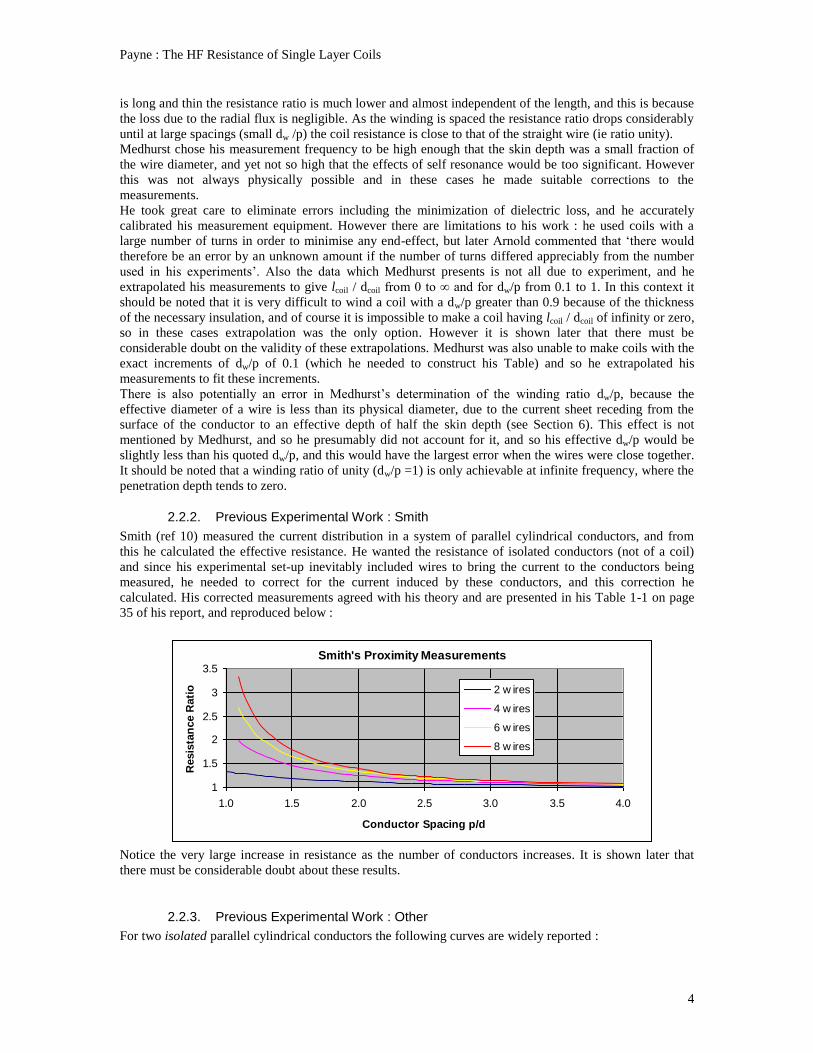
Smith (ref 10) measured the current distribution in a system of parallel cylindrical conductors, and from

this he calculated the effective resistance. He wanted the resistance of isolated conductors (not of a coil)

and since his experimental set-up inevitably included wires to bring the current to the conductors being

measured, he needed to correct for the current induced by these conductors, and this correction he

calculated. His corrected measurements agreed with his theory and are presented in his Table 1-1 on page

35 of his report, and reproduced below :

Smith's Proximity Measurements

1

1.5

2

2.5

3

3.5

1.0 1.5 2.0 2.5 3.0 3.5 4.0

Conductor Spacing p/d

Resis

tan

ce R

ati

o 2 w ires

4 w ires

6 w ires

8 w ires

Notice the very large increase in resistance as the number of conductors increases. It is shown later that

there must be considerable doubt about these results.

2.2.3. Previous Experimental Work : Other

For two isolated parallel cylindrical conductors the following curves are widely reported :


5

The origin of the data for in-phase currents seems to be from Butterworth (ref 11), and was therefore

theoretical, not measured. However, Smith’s data for 2 wires is virtually identical, and he claims to have

supported his work with measurements. However, this cannot be true for p/d=1 because he was unable to

measure for p/d greater than 0.9 because of the impossibility of inserting a current probe in a zero width

gap.

3. DERIVING THE MAGNETIC FLUX INTENSITY FROM NAGAOKA

It is shown in this section that the strength of the axial and the radial fields can be derived from Nagaoka’s

factor.

The inductance of a very long single layer coil is given by :

L ≈ μo N2 A / l coil 3.1

where N is the number of turns.

A is the area of the coil cross-section

lcoil is the length of the coil

The above equation is for a current sheet, but is applicable to a wound coil if there are many turns close

wound. The equation is approximate because there is leakage of the flux through the sides of the coil close

to each end. If the coil is sufficiently long this leakage is a small percentage of the total and can be

neglected. If the coil is not long and thin (the normal case) then a correction must be applied as follows :

L = [ μo N2 A / lcoil] Kn 3.2

Here the equation has been multiplied by Nagaoka’s factor Kn, and the values for this are commonly

tabulated because the underlying equations are complicated. A plot of the values given by Grover (ref 5) is

given below:

Nagaoka Factor

0

0.2

0.4

0.6

0.8

1

1.2

0.01 0.10 1.00 10.00 100.00

Coil Length/Dia

Kn

Nagaoka (from Grover)

Welsby Approx


6

Notice that its value is never more than unity. Also shown is the following empirical equation due to

Welsby ( ref 6) :

Kn ≈ 1/ [ 1+ 0.45 (dcoil / lcoil) - 0.005 (dcoil / lcoil)2 ] 3.3

Where dcoil is the coil diameter, and lcoil its length

This equation agrees with the tabulated values to within ±1.5% for lcoil /dcoil from 0.05 to ∞. For lcoil /dcoil

less than 0.05, an exact equation is given by Grover ( ref 5), Kn = 2/π lcoil / dcoil [Ln (4dcoil / lcoil) - 0.5).

The significance here of Kn, is that it accurately describes the relative strength of axial flux down the coil.

This arises because the inductance is given by L= Φ/I where Φ is the axial flux and I the current. So if the

total flux is Φt then axial flux as a proportion of this will be :

Φaxial / Φt = Kn 3.4

The radial flux will then be, as a proportion of the total flux :

Φradial / Φt = (1-Kn ) 3.5

The loss due to this radial flux is proportional to that component which is normal to the conductor. No

equation is known for this angle, but the flux lines intercept the conductor at a very shallow angle when the

coil is long and thin (0o when infinitely long), and at an angle close to 30

o when short and fat so the normal

component is then 0.5. We can anticipate that the angle is related to the hypotenuse of a triangle of sides

dcoil and lcoil, and a simple empirical equation for the normal component which meets these criteria is :

Φnormal / Φt ≈ (1-Kn ) M 3.6

where M = dcoil /[ (2 dcoil)2 + ( lcoil)

2]

0.5

Nagaoka’s factor also tells us another important factor, and that is the mean length of the coil over which

the radial flux intercepts the conductor. To calculate this it is instructive to rewrite equation 3.2 in the

following form :

L = μo n2 A lcoil Kn 3.7

Here n is the number of turns per metre. In this form we see that the effective length of the coil is Kn lcoil,

so the apparent length of coil which does not contribute to the axial flux, equal to the average length over

which the radial field intercepts the conductor, lintercept, is :

l intercept = [1- Kn ] lcoil 3.8

Notice that the intercept length at each end of the coil, is half the above value

The above relationships can now be used to calculate the loss in the conductor, and this is given in the next

section.

4. RESISTANCE OF A COIL WOUND WITH THIN CONDUCTING STRIP

4.1. Current Sheet

The loss calculated in this section is for a coil wound with a flat conducting strip. This could have many

turns N, or in the limit be a single turn wound with a strip of length 2πacoil and width lcoil. The strip is


7

assumed to have a thickness very much smaller than its width but of many skin depths so that the Rwall

concept can be used (Appendix 1). The effects of winding with round wire are considered in Section 5.

The total resistance is defined here as :

Rtotal = Ro + RA + RR 4.1.1

Ro is the resistance of the unwound conductor, and RA and RR are the added resistance due to the axial and

radial fields respectively. There is an assumption here that there is no interaction between these loss

components, and the same assumption is made by both Butterworth and Arnold. This seems to be

essentially true, at least to the uncertainty of any measurements which have been undertaken.

The resistance Ros (the suffix s indicates this is for strip, to distinguish it from round wire) is equal to the

surface resistivity Rwall multiplied by the conductor length and divided by its width (see Appendix 1).

Ros =Rwall [(2π acoil N)2 + l coil

2]

0.5 / [2 (w +t)] 4.1.2

This assumes that for this unwound strip conductor all surfaces carry the current, so that the perimeter is 2

(w+t). This equation ignores the increase in loss due to the current crowding across the width of a straight

strip conductor (see Appendix 1), but this crowding is absent when the strip is close-wound into a coil, and

so the above equation is more useful for the purpose of comparison

When this strip is close wound into a coil with N turns, the edges now carry no current except the two at the

ends, and so the factor (w+t) in the above equation becomes {w+t/N}. In general t/N is very small

compared with w and so can be ignored. For the wound coil it is convenient to express Ros in terms of the

pitch of the winding, w/p, and for a coil wound with N turns of strip of width w, then w= l coil (w/p) / N,

and the above equation becomes :

Ros =Rwall [(2π acoil N)2 + l coil

2]

0.5 N / [2 l coil (w/p) ] 4.1.3

If (2π acoil N)2 >> l coil

2 (the normal case ), then :

Ros ≈ Rwall 2π acoil N2 / [2 l coil (w/p) ] 4.1.4

4.2. Loss due to Axial Flux RA

To determine the loss due to the axial flux, the conductor is assumed to be a cylindrical current sheet of

negligible thickness and so axial flux does not cut it and so produces no additional loss. However, when

close wound into a long thin coil the current flows only on the inside face of the conductor, compared with

the two faces when it is unwound and straight. So the resistance doubles, or in terms of Equation 4.1.1, RA

= Ros. It is found that as the coil is made shorter and fatter the current begins to flow also on the outer

surface, and when the coil is very short both surfaces are nearly fully conducting, and RA tends towards

zero. This effect is proportional to the axial flux and so we have:

RA = Ros Kn2 4.2.1

4.3. Loss due to Radial Flux

To calculate the loss due to the radial field it is convenient initially to consider a coil made from a single

turn of strip. The total magnetic intensity due to a current Iin flowing in this winding is :

HT = Iin / lc 4.3.1

Where lc is the length of the magnetic path, and this is approximately equal to lcoil, ignoring any slight

curvature of the field lines.

From Equation 3.6 the radial intensity HR is given by :

HR = HT (1- Kn ) M


8

And substituting Equation 4.3.1:

HR = (Iin / lc)(1- Kn ) M 4.3.2

This radial intensity will induce a current in the coil Iend, within the distance l intercept / 2 at each end

(Equation 3.8), and this current will generate a field intensity HE which will be equal in magnitude to HR

(assuming the conductivity is high) and oppose it. So we can write :

HE = Iend /le 4.3.3

Where le is the length of the magnetic path. This is approximately equal to lcoil – l intercept , again ignoring

any curvature of the field lines.

Equating equations above we get :

Iend / Iin= (1- Kn ) M (le / lc) 4.3.4

This current will produce a power loss I2end Rend, where Rend is equal to Rwall multiplied by the current path

length and divided by its width. To find the length of the current path and its width, consider the intercept

cylinder at one end of the coil of length l intercept /2, as being flattened out into a plate of width l intercept /2 and

length 2π acoil. If we imagine this strip is divided into two, each of width 0.5 (l intercept /2) and a current of Iend

flowing in one direction along one half strip and in the other direction along the other half strip this will

produce the required magnetic field intensity. Taking these half strips and forming them back into cylinders

we have two cylinders side by side each carrying a current of Iend but in opposite directions. Thus any axial

flux from one cylinder is cancelled by that from the other, but together they form a couple producing a

radial field HE, normal to the conductor. The loss resistance of these two cylinders will be :

Rend = Rwall * 2 (2π acoil)/ [0.5 ( l intercept /2)] 4.3.5

= Rwall * 16π acoil / l intercept

The above assumes that the strip is many skin depths thick so current flows on only the inside of the strips

(ie one side) .

The power lost will then be (for two ends) :

Pends = 2 I2

end Rend

= 2 I2end Rwall * 16π acoil) / l intercept 4.3.6

This must be equal to the input power I2in Rin, and equating this with the above equation and substituting

Equation 4.3.4 for Iend / Iin we get :

RR = Rwall 32 π (1- Kn )2 M

2 (le / lc)

2 (acoil) / l intercept 4.3.7

Ignoring any small curvature of the flux lines, lc is approximately equal to lcoil, and le is approximately equal

to lcoil – l intercept . Since l intercept = [1- Kn ] lcoil then le / lc ≈ Kn , and this gives a good estimate when the coil

is long and thin. However when the coil is short, we need to allow for this curvature, and this seems to be

about 5% when lcoil /dcoil is unity, giving the following empirical equation :

(le / lc) ≈ Kn (1+ 0.05 dcoil / lcoil ) 4.3.8

If the coil consists of N closely spaced turns, the length of this strip conductor will increase by N and its

width reduce by N, so the resistance increases by N2, and if the turns are spaced the width further reduces

by w/p, where w is the width of the strip and p the pitch, so the resistance increases by p/w. In addition the


9

radial flux cutting the conductor is now reduced by w /p, and the resistive loss reduces as the square of the

flux ie as (w /p)2. So Equation 4.3.7 becomes :

RRS = Rwall N2 32 π (1- Kn ) (w /p) M

2 (le / lc)

2 (acoil / l coil ) 4.3.9

4.4. Overall Loss

From equations 4.1.1, 4.2.1 and 4.3.9, the overall loss for conducting strip is :

Rtotal = Ros + Ros Kn2 + Rwall N

2 32 π (1- Kn ) (w /p) M

2 (le / lc)

2 (acoil / l coil ) 4.4.1

where Ros ≈ Rwall 2π acoil N2 / [2 l coil (w/p) ]

Rwall = ρ / δ where ρ is the resistivity of the conductor and δ the skin depth

M ≈ dcoil /[ (2 dcoil)2 + ( lcoil)

2]

0.5

Kn ≈ 1/ [ 1+ 0.45 (dcoil / lcoil) - 0.005 (dcoil / lcoil)2 ]

(le / lc) ≈ Kn. (1+ 0.05 dcoil / lcoil )

acoil and l coil the radius and length of the coil.

4.5. Normalised Loss

The loss can be expressed as the ratio of the coil resistance to that of the unwound strip conductor Ros. So:

Rtotal / Ro = (1+ RAs / Ros + RRs / Ros ) = (1+ Kn2 + RRs / Ros ) 4.5.1

where RRs is given by equation 4.3.9

Ros is given by equation 4.1.4

This equation is plotted below for w/p = 0.75:

Conducting Tape - Comparison with Theory

1.0

1.2

1.4

1.6

1.8

2.0

2.2

0 1 2 3 4 5 6 7 8 9 10Coil Length/Dia

Resis

tan

ce R

ati

o

Theoretical w /p=0.75

Measured, 26 turns, plastic, w /p=0.75

Measured, 5 turns, plastic, w /p =0.75

No published measurements are known for coils wound with tape, and so the theory was tested with two

coils made by the author, one with a very small lcoil /dcoil, and the other larger lcoil /dcoil. The measurements

on these are shown above and reported in Appendices 3 and 4, and give some support for the theory here.

In comparing theory with experiment above it should be noted that the resistance values are very low here

(around 0.35Ω) and thus susceptible to large measurement error, estimated at ±11%, and shown as error

bars above.


10

5. RESISTANCE OF A COIL WOUND WITH CIRCULAR WIRE

5.1. Introduction

In this section the analysis is expanded to cover the loss in a coil wound with a conductor of circular cross-

section. The resistance of the wire unwound and straight is designated by Row , to distinguish it from the

unwound strip Ros, and if the skin depth is a small fraction of the wire diameter this resistance is equal to

the surface resistivity Rwall multiplied by the conductor length and divided by its effective perimeter (see

Appendix 1). For a coil wound with wire of diameter of dw :

Row =Rwall [(2π acoil N)2 + l coil

2]

0.5 / (π dw) 5.1.1

If (π dcoil N)2 >> l coil

2 (the normal case ), then :

Row ≈ Rwall 2 acoil N / dw 5.1.2

It is convenient to express this in terms of the spacing of the winding dw/p, and for a coil wound with N

turns of wire, then dw = l coil (dw /p) /N , and the above equation becomes :

Row ≈ Rwall 2 acoil N2 / [l coil (dw /p)] 5.1.3

The overall loss is as given by Equation 4.1.1, repeated below :

Rtotal = Row + RAw + RRw 5.1.4

And when normalised to the unwound straight wire:

Rtotal / Ro w = 1 + RAw/ Ro w + RRw / Ro w 5.1.5

5.2. Loss due to Axial Flux

As with the strip conductor the current flows on the inside surface only when the coil is long and thin but

on both surfaces when short and fat. However, unlike the strip conductor, the cylindrical conductor is

intercepted by the axial flux, and this leads to an additional loss. This loss is proportional to the square of

the flux and so from Equation 3.4 :

RAw = (Row kr) Kn2 5.2.1

where Kn is given by Equation 3.3.

The factor (Row kr ) is the loss resistance RAw when the radial field is negligible (RRw =0) and Kn =1, and

this occurs when lcoil /dcoil is infinite. For these conditions and combining the above equation with Equation

4.1.2 gives :

Rtotal = (1 + kr) Row 5.2.2

The total loss due to the axial flux for an infinitely long coil is given by Equation A2.14 and when

normalised to the unwound wire by Equation A2.15. This latter equation gives the following values for

increments in dw/p of 0.1 :


11

dw/p 1+ kr

1 3.46

0.9 3.15

0.8 2.83

0.7 2.51

0.6 2.21

0.5 1.92

0.4 1.65

0.3 1.42

0.2 1.23

0.1 1.08

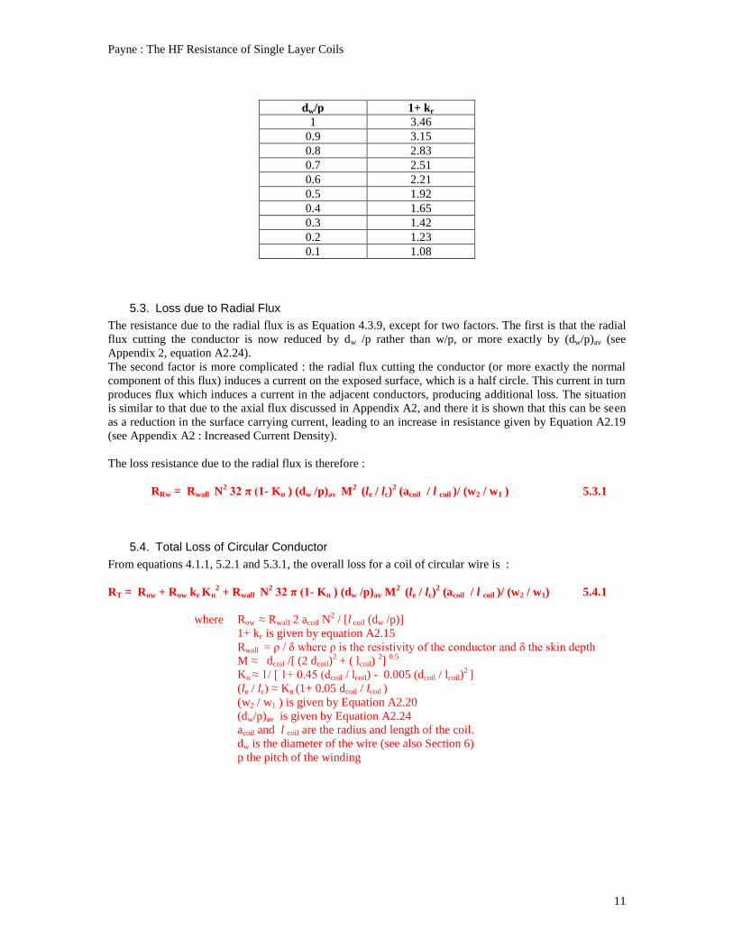
5.3. Loss due to Radial Flux

The resistance due to the radial flux is as Equation 4.3.9, except for two factors. The first is that the radial

flux cutting the conductor is now reduced by dw /p rather than w/p, or more exactly by (dw/p)av (see

Appendix 2, equation A2.24).

The second factor is more complicated : the radial flux cutting the conductor (or more exactly the normal

component of this flux) induces a current on the exposed surface, which is a half circle. This current in turn

produces flux which induces a current in the adjacent conductors, producing additional loss. The situation

is similar to that due to the axial flux discussed in Appendix A2, and there it is shown that this can be seen

as a reduction in the surface carrying current, leading to an increase in resistance given by Equation A2.19

(see Appendix A2 : Increased Current Density).

The loss resistance due to the radial flux is therefore :

RRw = Rwall N2 32 π (1- Kn ) (dw /p)av M

2 (le / lc)

2 (acoil / l coil )/ (w2 / w1 ) 5.3.1

5.4. Total Loss of Circular Conductor

From equations 4.1.1, 5.2.1 and 5.3.1, the overall loss for a coil of circular wire is :

RT = Row + Row kr Kn2 + Rwall N

2 32 π (1- Kn ) (dw /p)av M

2 (le / lc)

2 (acoil / l coil )/ (w2 / w1) 5.4.1

where Row ≈ Rwall 2 acoil N2 / [l coil (dw /p)]

1+ kr is given by equation A2.15

Rwall = ρ / δ where ρ is the resistivity of the conductor and δ the skin depth

M ≈ dcoil /[ (2 dcoil)2 + ( lcoil)

2]

0.5

Kn ≈ 1/ [ 1+ 0.45 (dcoil / lcoil) - 0.005 (dcoil / lcoil)2 ]

(le / lc) ≈ Kn (1+ 0.05 dcoil / lcoil )

(w2 / w1 ) is given by Equation A2.20

(dw/p)av is given by Equation A2.24

acoil and l coil are the radius and length of the coil.

dw is the diameter of the wire (see also Section 6)

p the pitch of the winding


12

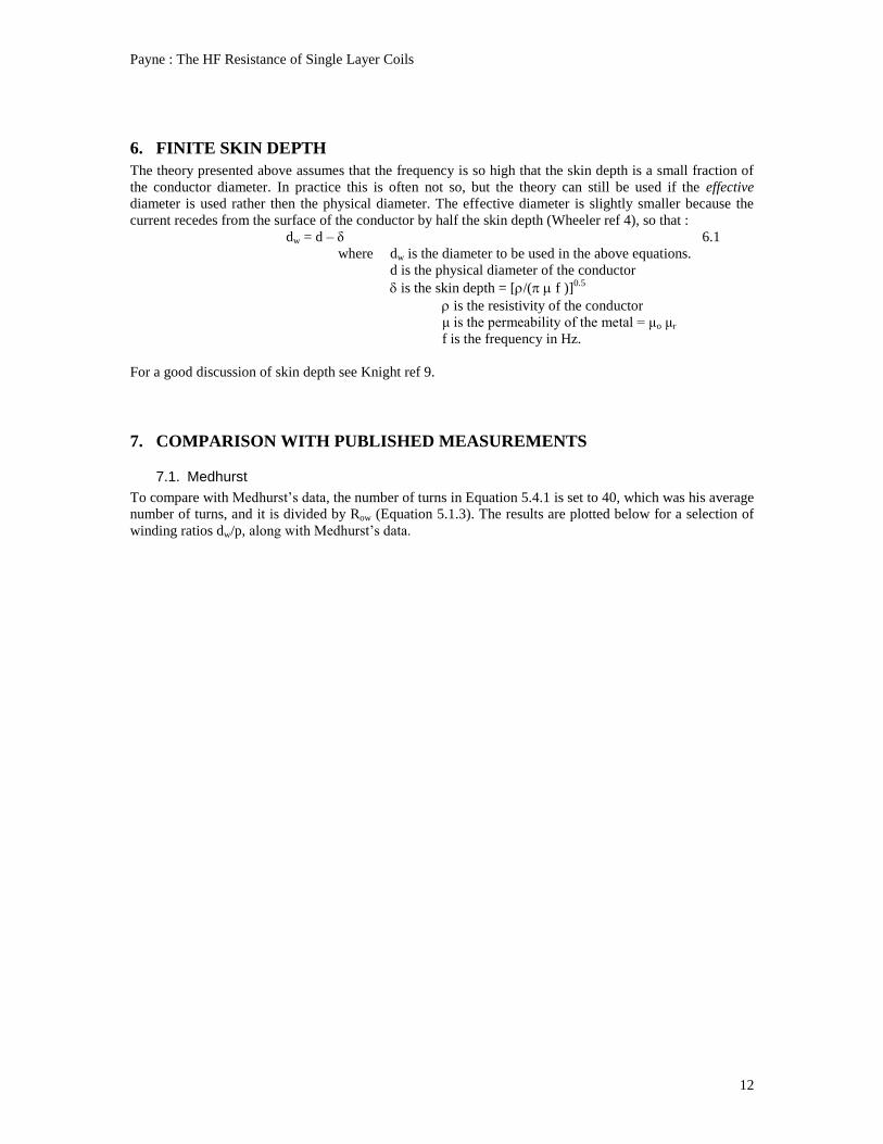
6. FINITE SKIN DEPTH

The theory presented above assumes that the frequency is so high that the skin depth is a small fraction of

the conductor diameter. In practice this is often not so, but the theory can still be used if the effective

diameter is used rather then the physical diameter. The effective diameter is slightly smaller because the

current recedes from the surface of the conductor by half the skin depth (Wheeler ref 4), so that :

dw = d – δ 6.1

where dw is the diameter to be used in the above equations.

d is the physical diameter of the conductor

is the skin depth = [/( f )]0.5

is the resistivity of the conductor

μ is the permeability of the metal = μo μr

f is the frequency in Hz.

For a good discussion of skin depth see Knight ref 9.

7. COMPARISON WITH PUBLISHED MEASUREMENTS

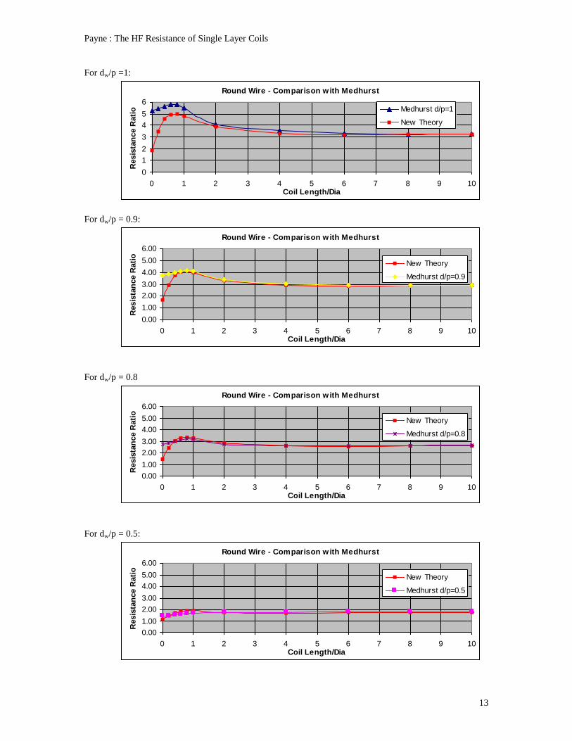
7.1. Medhurst

To compare with Medhurst’s data, the number of turns in Equation 5.4.1 is set to 40, which was his average

number of turns, and it is divided by Row (Equation 5.1.3). The results are plotted below for a selection of

winding ratios dw/p, along with Medhurst’s data.


13

For dw/p =1:

Round Wire - Comparison with Medhurst

0

1

2

3

4

5

6

0 1 2 3 4 5 6 7 8 9 10Coil Length/Dia

Resis

tan

ce R

ati

o Medhurst d/p=1

New Theory

For dw/p = 0.9:


0.00

1.00

2.00

3.00

4.00

5.00

6.00

0 1 2 3 4 5 6 7 8 9 10Coil Length/Dia

Resis

tan

ce R

ati

o

New Theory

Medhurst d/p=0.9

For dw/p = 0.8


0.00

1.00

2.00

3.00

4.00

5.00

6.00

0 1 2 3 4 5 6 7 8 9 10Coil Length/Dia

Resis

tan

ce R

ati

o

New Theory

Medhurst d/p=0.8

For dw/p = 0.5:


0.00

1.00

2.00

3.00

4.00

5.00

6.00

0 1 2 3 4 5 6 7 8 9 10Coil Length/Dia

Resis

tan

ce R

ati

o

New Theory

Medhurst d/p=0.5


14

The calculated values are generally within ±5% of Medhurst’s values for lcoil / dcoil from 0.4 to ∞ and for all

values of dw/p. The exception is dw/p=1 where the difference is much larger, and the most likely source of

error here is in Medhurst’s extrapolation given that the correlation is so good for all other values of dw/p.

For lcoil / dcoil ratios less than 0.4 there is a very large discrepancy, with the theoretical curves tending

towards unity for lcoil / dcoil = zero, and Medhurst’s curves tending towards a much higher ratio of around

90% of the peak value. Again the error is likely to be in Medhurst’s extrapolation, since experiments by the

author support the theoretical values (see Appendices 3 & 4), at least down to values of lcoil / dcoil = 0.03

(Section 7.3). The equations start to break down at lower values, but the basic theory here is based on

Nagaoka’s factor and this goes to zero for a coil of infinite diameter, implying the resistance ratio goes to

unity. Experiment does not support this and so there must be an additional flux, not included in Nagaoka’s

factor, and this is likely to be the flux around the individual wires.

7.2. Comparison with Smith’s Data

Smith (ref10) purports to give the proximity loss of isolated conductors. However the following suggests

that his data is consistent with the loss of conductors forming a coil, rather than isolated.

If Smith’s parallel wires were indeed isolated as he intended, then his wires when very close together, and

all carrying current in the same direction, could be approximated by a single isolated rectangular conductor.

So if there are N wires each having a diameter dw, then the equivalent rectangle has a thickness dw and

width Ndw. Equation A1.5, for the resistance ratio of an isolated conducting strip, can then be used to

estimate the resistance ratio, and gives the following results :

Proximity Effect w ith Multiple Conductors d/p=0.91

1

1.5

2

2.5

3

3.5

2 3 4 5 6 7 8 9

Number of Conductors

Resis

tan

ce R

ati

o Smith

Flat Strip Approximation

The difference is very large, and although the single rectangular conductor is an approximation it would be

very surprising if the close parallel wires differed markedly from this.

So his data is not consistent with isolated wires. However if we assume that Smith’s attempts to cancel the

effects of his leads were not successful, so that his results are that of a coil, then his data agrees rather better

with the theory presented here, as shown below:

Comparison with Smith's 'coil'

1

1.5

2

2.5

3

3.5

4

0.00 0.05 0.10 0.15 0.20 0.25 0.30

Coil Length/dia

R/R

o

Smith d/p=0.91

New Theory d/p=0.91


15

In the above, Smith’s number of wires was converted to an equivalent lcoil / dcoil for a coil, using the

dimensions he gives for his conductors and his feed circuits. These formed square loops and it was assumed

that the equivalent circular loop had the same area. His feed wires were wire braid rather than the round

tubes used for his current measurements, but inherent in the use of the theory here is the assumption that all

conductors have the same diameter. Also it was assumed that his feed wires had the same distance apart as

the conductors being measured, but it is not clear whether this is true from his description. The correlation

is surprisingly good given these assumptions.

Taken together the above two graphs place considerable doubt on Smith’s data, and suggest that his

measurements were of a coil rather than the isolated conductors as he intended. If this conclusion is right

then his theoretical cancellation of his feed circuits was far from complete, and a re-reading of his

(complicated) paper suggests that he did not compensate adequately for the axial flux down the coil.

7.3. Proximity Resistance of 2 Conductors

The published data for the proximity resistance of two parallel conductors (Section 2.5) is based on

Butterworth’s theory (ref 11) for isolated conductors. That is, for conductors where the return path is an

infinite distance away. Smith’s measurements gave exactly the same results, but there has to be some doubt

about these as discussed above.

Butterworth’s data is shown below along with the result of a single experiment by the author, where the

return path was a large distance away compared with the diameter of the conductor, but not infinite

distance (see Appendix 5).

Proximity 2 w ires

1

1.1

1.2

1.3

1.4

1.5

1.6

1 2 3 4


Resis

tan

ce R

ati

o Smith & Butterw orth

Payne measurementNew Theory (L/D = 0.03)

Also shown is the theoretical prediction for lcoil / dcoil = 0.03, which is the equivalent coil ratio to that of the

experiment The agreement with experiment is within 2%, although this is likely to be fortuitous given the

measurement uncertainty.

The agreement between Butterworth and experiment appears less favourable, but is just within

experimental error.

The theory predicts lower values of the resistance ratio for smaller values of lcoil / dcoil (ie the return

conductor farther away) and this does not correspond with experiment, and is a limitation of the theory

here.

8. DISCUSSION

Overall the agreement with Medhurst’s measurements is very good, generally within 5%. However the

agreement with his extrapolations is very poor, particularly for very short coils, and in contrast the author’s

own measurements support the theory given here. These measurements are described in some detail

(Appendices 3 and 4) because they give such different results to Medhurst that they could be open to doubt.

The other area of disagreement is for dw/p=1, but it has not been possible to verify the theory for this ratio

because of the impossibility of winding a coil with zero gap between turns, or even a near-zero gap.

There is good agreement with experiment for the proximity loss for two conductors, but less good with

Butterworth’s theoretical data.


16

Smith’s data for multiple parallel isolated conductors is not at all in agreement with the theory given here.

However, if it is assumed that Smith’s measurements are of a coil, rather than isolated conductors as he

intended, then his measurements are consistent with the theory.

The analysis presented here has a theoretical basis except for three equations which are empirical, and these

are : a) the value of M in Equation 3.6, b) the value of x in Equation A2.14, and c) the curvature factor in

Equation 4.3.8. These equations have some credibility in that each is based upon the known shape of the

magnetic field within a coil, each is very simple, and also they are supported by the overall good

correlation with Medhurst’s measurements, and the author’s experiments. Clearly it would be preferable for

them to have a firm theoretical basis.

One interesting result from the theory is that in long close-wound coils the current flows essentially on the

inside surface of the conductor (be this round wire or tape), and this result is well known. However as the

coil is made shorter and fatter some conduction also occurs on the outside surface, and when the coil is

very short and fat it is essentially the whole of the conductor periphery carrying current.


17

Appendix 1 : Rwall

This Appendix describes the concept of surface resistance, or wall resistance, Rwall.

The d.c. resistance of a conductor is given by the well known equation :

Rdc = ρ l / A A1.1

where is the resistivity of the conductor

l is the length of the conductor

A is its area

At high frequencies the current decays exponentially as it penetrates the conductor from the outside, and

this is equivalent to current flowing in only a thin skin on the surface of the conductor, of depth . The

conducting area is therefore dw, and inserting this into A1.1 gives :

Rcircle = [ρ /] [l / ( dw) A1.2

where is the skin depth = [/( f )]0.5

μ is the permeability of the metal = μo μr

f is the frequency in Hz.

The ratio (ρ /) is called Rwall, and so we have :

Rcircle = Rwall l / ( dw) A1.3

where Rwall = / = ( f )0.5

If the conductor is a thin strip of rectangular cross-section of width w and thickness t, then its perimeter is

2( w+ t) and we could expect the high frequency resistance to be given by :

Rstrip = Rwall l / [2( w+ t)] A1.4

This equation would be true if the current density was constant across the width, but in fact it crowds

towards the edges, and this raises the resistance by a factor of between 1.27 and 2 for ratios of w/t between

1 and 100. An equation which agrees with the author’s experiments to better than 5% (see Appendix 3) is

given by multiplying the above equation by :

Kfringing = 1.06 +0.22 Ln w/t +0.28 (t/w)2 A1.5

This equation is from reference 7. Terman (page 35) also gives a curve which corresponds to this equation.

For hard drawn copper wire = 1.77 x 10 –8

at 200C and = 4 x 10

–7 and so the skin depth at 20

0C is

given by:

Skin depth in copper = 66.6/ f^0.5

mm A1.6

Where f is in Hz


18

Appendix 2 : (RA/Row )∞

This Appendix considers the loss ratio in a coil wound with circular wire when there is no loss from the

radial field and the axial field is a maximum (i.e. Kn =1), and this occurs when lcoil / dcoil equals infinity.

Taking equation 5.1.5, with RRw / Ro w =0 :

Rtotal∞ / Row = 1+ (RA/Row )∞ A2.1

The infinity suffix indicates that this is for lcoil / dcoil = ∞

Two authors have given values when dw/p=0.9. Medhurst gives 1+ (RA/Row)∞ = 3.11, and this is an

extrapolation of his experimental data. Wheeler gives a calculation for square section wire which he then

suggests is applicable to ‘practical coils wound with circular wire with a diameter slightly less than the

pitch of the winding’ (presumably dw/p ≈ 0.9) and gives a value of 1+ (RA/Row )∞ = 3.14. So these are

within 1% of one another.

For dw/p =1, there is only limited data and Medhurst gives 1+ (RA/Row )∞ = 3.41, but again this value is

from his extrapolation of his experimental data. He does not give his method of extrapolation and other

extrapolations to a higher or lower figure seem equally justifiable.

Below is given a theoretical derivation based upon the magnetic intensity at the surface of one conductor

due to current flowing in its neighbours. This gives a value which is dependent upon the number of turns,

and for infinite turns (since lcoil / dcoil is infinite) and dw/p=1, this gives a value of 1+ (RA/Row )∞ = 3.46,

slightly greater than Medhurst’s value. However if we assume 40 turns, which is the average number which

Medhurst used in his experiments and from which he did his extrapolations, the theory here gives a value of

3.42, which is within 0.3% of Medhurst’s value.

Consider two adjacent wires, A and B with a distance between centres of p as above. The flux from each

wire can be considered as being generated by a thin filament carrying a current I situated at the wire

centres.

There will be a current induced in the surface of wire A by the field from wire B, and this will produce

eddy currents in the surface of wire A, giving a power loss. This power loss must come from wire B and so

its apparent resistance will increase. This power loss can be determined from the magnetic intensity on the

surface of wire A due to the current in B, and this intensity is given by :

a r

n

t

x

p

Wire A Wire B o


19

HAB = IB/ r’ A2.2

Where r’ is the component of r normal to the surface, and equal to n/r. So:

HAB = IB (n/ r2) A2.3

To calculate the power loss which this produces we note that for filament A carrying the current I, the

magnetic intensity at its surface, at radius a, is HAA = I A/ a, and this intensity gives rise to a power loss (in

the absence of any wires nearby) of :

P0 = IA2 Rwall * l wire / (2π aw) A 2.4

So if IA = IB =I the loss induced at any point on the surface of wire A, by the field from wire B will be :

P = (HAB /HAA)2 I

2 Rwall * l wire / (2 π aw )

= [I (n aw)/ r2]

2 Rwall * l wire / (2π aw ) A2.5

So the total power will be equal to the above equation, integrated over the angle over which the current is

induced. From the above diagram this is from θ =0 to θ1, where θ1 is the angle of a when r is tangential to

the wire surface, so that θ1 = Cos-1

(p/dw). So the total induced power is :

θ1

Pinduced = Rwall * l wire / (π dw) I2 ∫ [(n aw)/ r

2]

2 dθ A2.6

0

To calculate (n/ r2), then from the diagram above :

r = [o2 +(p-x)

2]

0.5 A2.7

where o= aw Sin θ

x= aw Cos θ

θ is the angle of a to the baseline between centres

n= [r2-t

2]

0.5 A2.8

where t=p Sin θ

So from the above :

n/r2 = [r

2-t

2]

0.5/ r

2

= [o2 +(p-x)

2 – (p Sin θ)

2]

0.5/ [o

2 +(p-x)

2]

= [(aw Sin θ)2 + (p – awCos θ)

2 – ( p Sin θ)

2]

0.5/[ (awSin θ)

2 + (p – awCos θ)

2] A2.9

To find the total power lost we need to determine the integral in Equation A2.9 and this has been done

numerically, with aw=1, to give :


20

dw/p (IMS /I2 )

1 0.364

0.9 0.296

0.8 0.231

0.7 0.172

0.6 0.122

0.5 0.082

0.4 0.048

0.3 0.026

0.2 0.011

0.1 0.003

θ1

In the above, (IMS /I2 ) = ∫ [(n aw)/ r

2]

2 dθ

0

where IMS is the mean square current. An empirical equation which matches the above to 2% is :

(IMS /I2) ≈ 0.0026 – 0.04 dw/p + 0.404 (dw/p)

2 A2.10

To calculate the total power lost in the conductor it is convenient to firstly consider when dw’/p =1. Then

the total power lost will be due to two components :a) the current I flowing in only the half circle of wire

facing the axis of the coil, plus b) the loss due to the adjacent conductors. All conductors have two adjacent

wires except the two on the end and so this aspect of loss must be multiplied by 2 (N-1)/N, where N is the

total number of turns. So :

P total = I2 Rwall *[ l wire /aw ] [1 /π + 2 {(N-1)/N} (IMS /I

2) / π] A2.11

Now for dw’/ p= 1, IMS /I =0.364 (from the table above, or equation A2.10). Also setting N to infinity,

(because an infinitely long coil must have an infinite number of turns), we get :

P d/p=1 = I2 Rwall *[ l wire /aw] [1 /π + 0.728 / π]

= I2 Rwall *[ l wire /aw] [ 1.728/π] A2.12

The power lost in the unwound wire will be P total = I2

Rwall *[ l wire /(2π aw)] and the ratio of these gives the

increase in resistance when coiled :

1+ (RA/Row )∞ = 3.46 for dw/p= 1 and N=∞ A2.13

We now consider the case where the coil is still infinitely long but dw’/ p is less than 1. As the wires are

moved apart, the conducting angle increases from π (i.e. the half surface adjacent to the coil axis) to a value

π (1+ x), with a corresponding reduction in the resistance. The loss due to the induced current will increase

by the same factor (1+x). As to the value of x, we can anticipate that this will be dependent upon the gap

between the wires, (p- dw’), normalised to the pitch, and indeed this gives good agreement with Medhurst’s

experimental values. So x≈ (p - dw)/p giving :

P d/p = I2 Rwall *[ l wire /aw ] [1 /{ π (1+x)} + 2 (N-1) (1+x) /N (IMS /I

2) / π] A2.14

Where x ≈ (p - dw)/p = (1- dw/p)

Normalising to the power lost in the unwound wire P total = I2 Rwall *[ l wire /(2π aw)] gives :


21

1+ (RA/Row )∞ = 1+ kr = 2π [1 /{ π (1+x)} + 2 (N-1) (1+x) /N (IMS /I2) / π] A2.15

This gives the following compared with Medhurst :

Loss Resistance for L/D = Infinity

1

1.5

2

2.5

3

3.5

0 0.1 0.2 0.3 0.4 0.5 0.6 0.7 0.8 0.9 1

d/p

R/R

o

Medhurst

Theoretical

The theoretical curve is within 5.5% of Medhurst’s extrapolated values.

It should be noted that in the above analysis it is not necessary to consider the effect of flux on wires other

than the two adjacent ones, because the flux beyond the adjacent wires is reduced to zero by the surface

currents induced into the adjacent wires.

Increased Current Density

Another way of looking at the above problem is that the field from conductor B reduces the conducting

area in conductor A because the induced eddy current negates some of its surface current. So the current I

flowing on the surface of A now has to flow in a constrained periphery, with the result that the current

density increases and thus the loss.

If we call the total periphery w1 then the power lost is :

P1 = I12 Rwall l1 / w1 A2.16

And the power lost in the constrained periphery w2:

P2 = I22 Rwall l1 / w2 A2.17

Now I1 = I2 and l1= l2 so

P1 / P2 = w2 / w1 A2.18

From equation A2.14 :

P2 = (P1 + Pinduced ) = P1 [1+ 2 (N’-1) /N’(IMS /I2)] A2.19

Here N’ is the number of turns over the intercept distance l intercept = [1- Kn ] lcoil , so N’=N [1- Kn ]

The ratio of the conducting periphery to the total periphery is therefore :

w2 / w1 = 1/ [1+ 2 (N’-1) / N’(IMS /I2)] A2.20

where N’=N [1- Kn ]

Average Pitch

From the above it is seen that the effective conducting periphery is reduced by the adjacent conductors.

Most conductors in the coil have conductors on each side and so this reduction is symmetric about their


22

centre, and the pitch is unchanged. This is not so for the two end conductors which have an adjacent

conductor on one side only and this has the effect of increasing the pitch between the end conductor and its

neighbour. This is particularly noticeable when the number of turns is small, especially when there are just

two conductors.

This increase in pitch can be estimated from the reduced periphery, equation A20.20 :

(w1/w2) =1/(1+Ims/Im2) A2.21

This reduction in effective periphery reduces the projected width of the wire to dwe given by :

dwe = dw (0.5+0.5Cos θ)

where θ =2π/(1+Ims/I2)

The centre of this projection is displaced from its neighbour by 0.5 (dw - dwe ) = 0.5 (dw - 0.5 dw - 0.5 dw Cos

θ). So the end pitch increases to :

p’ = p + 0.5 dw (1-Cosθ) A2.22

The average pitch for the whole coil will therefore be :

pav = [p (N-2) +2 p’]/N = p+ dw (1-Cosθ)/N A2.23

It is convenient to express this in terms of an average winding ratio and so we have :

(dw /p)av = [dw /p] / [ 1+( dw /p) (1-Cosθ)/N] A2.24

where θ=2π/(1+Ims/I2)

(IMS /I2) is given by equation A2.10

Appendix 3 : Measurements of Coils wound with Conducting Tape

There are no known measurements on the loss of coils wound with conducting tape, and so two coils were

made and measured in order to check the author’s theory. The first coil was designed to test the theory

when lcoil / dcoil was very small, and the second when lcoil / dcoil was large.

For both coils there were certain practical constraints. Firstly the resistance of the coils needed to be high

enough to allow accurate measurements (ideally >0.5 Ω). This meant that the conductor width should be

small and the measurement frequency high. However if the measurement frequency is too high it will come

close to the self resonant frequency (SRF), leading to measurement uncertainties. The SRF can be raised by

reducing the length of the conductor, but this then reduces the resistance, so this is of no advantage. It was

clear that a compromise was necessary, and it was decided to use a strip width of around 2 mm, a

measurement frequency around 4 MHz and a conductor length of around 1800 mm. For this strip length the

SRF was as low as 22 MHz (depending on the coil), and so its effect could not be ignored, and the

measured resistance values were corrected according to the following equation (see Welsby ref 6, p37) .

R = Rc [ 1- (f / fr )2]

2 A3.1

R is the low frequency value for the coil and Rc is the value measured at the frequency f, when there is a

self resonant frequency of fr. In all cases fr was measured, and defined as the frequency where the phase of

the input impedance passed through zero. For these fr measurements the circuit was the same as for the

resistance measurements, that is it consisted of the series circuit of the coil, the capacitor (see below) and

the connection leads. Strictly the above equation applies to the parallel resistance of the circuit, but is

applicable to the series resistance if the Q is high. Also the accuracy of this equation reduces as f / fr

approaches unity, so the measurement frequency should be as far away from the resonant frequency as

possible.


23

The reactance of the coils was very high compared to their loss (Q was as high as 290) and so to get

accurate resistance measurements it was necessary to tune out this reactance. This was done with a high

quality air dielectric variable capacitor, having silver plated vanes and contacts, and ceramic insulators and

connected in series with the coil. The loss of this capacitor has been measured by the author (ref 12) and the

series resistance is given by:

Rcap = [0.01+ 800 / (f C2) + 0.01(f

0.5) ] ±13% ohms A 3.2

where f is in MHz and C in pf.

The radiation resistance was of the order of 1 μΩ (depending on the coil) and so could be neglected.

All measurements were carried out with an Array Solutions AIM 4170 analyser, with the measurement jig

calibrated-out (with the capacitor shorted). The resistance values to be measured here are very low and the

measurements were subject to significant random variations due to quantising noise and to external noise

picked-up by the coils. This noise was reduced by using the analyser’s internal averaging function,

averaging 16 measurements at each frequency sweep, and also its smoothing facility to provide additional

averaging over 32 sweeps. Also the measurement frequency was chosen to avoid any strong transmissions

which could interfere with the measurements (detected on a communications receiver). Overall it is

difficult to assess the measurement uncertainty, but it is likely to be around ± 5%. To this must be added

the uncertainty in measuring the physical dimensions of the coil, including the winding pitch and strip

width, to give an estimated overall accuracy of ± 7%.

Conducting tape is more difficult to obtain than round wire. A number of suppliers have rolls of 5mm wide

tape with adhesive backing, and this makes it easy to fix the wire to the former. However most of these

tapes have very thin copper – around 0.03 mm, and this is only one skin depth at 4 MHz. Also the purity of

the copper is often not specified and any impurities could give some uncertainty on the conductivity and

skin depth. Because of these problems the author cut a 1.74 metre long strip from a sheet of high quality

copper, having a thickness of 0.25 mm, equivalent to 7.5 skin depths at 4 MHz. There were significant

variations in the width because the strip was cut by hand, and so this was measured at several points along

its length and varied from 2.08 to 2.38 mm, with a mean of 2.23 mm.

The coils were wound on plastic plumbing pipe (probably PVC), heated in an oven for several hours before

winding to remove moisture. Plumbing pipe is sometimes reported as being lossy, but the measured results

gave a good correlation with the theory, suggesting that the loss was not significant. One reason for the

high loss in some plastic pipe is that it is loaded with carbon to make it black, whereas the pipe used here

was light brown or white.

It was assumed that the resistivity of the copper was 1.71 10-8

Ωm at the measurement temperature of 16oC.

Measurements on ‘Straight’ Strip

Before the strip was wound into a coil its ‘straight’ RF resistance was measured. Of course it is not possible

to measure this except as a large single turn and this therefore had a diameter of around 554 mm. The

increase in resistance due to curvature is given by Wheeler (ref 4) as 1/ (D2- d

2)

0.5 for round wire. Assuming

in this case that d is equal to the strip thickness of 0.25 mm, then this equation gives an increase equal to a

very small fraction of 1%.

A measurement frequency of 5.4 MHz was used for this experiment because the SRF was quite high at 40

MHz. The resistance of the straight conductor was measured as 0.355 Ω after corrections for SRF, and the

calculated value using equations A1.4 and A1.5 was within 3.5% of this, although this is probably

fortuitous given the likely errors (see below).

Strip Coil with lcoil / dcoil = 0.134

The 1.74 meter strip was wound onto a large plastic plumbing pipe (light brown not black) with a nominal

diameter of 110 mm, giving 5 turns. There was an average spacing between turns of 0.73 mm, giving an

average pitch of 2.23+0.73= 2.96 mm, so giving the equivalent length of the current sheet as 5*2.96= 14.8

mm( see definition by Grover ref 5, p149), giving lcoil / dcoil = 0.134, and w/p=0.755. Measurements were

done at 4.04 MHz, and gave a resistance for the coil of 0.336 Ω after corrections. For comparison with the

theory the resistance of the straight conductor was calculated as 0.206 Ω, using Equation A1.4 only (since

the current crowding is absent when close wound into a coil). The ratio of these is 1.63, and Equation 4.4.1


24

gives 1.46 ( ie -10%). The error on these measurements is relatively large, mainly because the resistance is

such a low value and the analyser accuracy is not likely to be better than ± 10%. To this must be added the

uncertainty of ±13% in the capacitor resistance, and since this resistance is about 20% of the total this gives

an uncertainty of ±2.6%. So assuming these errors add in quadrature this gives an overall uncertainty of

11%. So the theory is within the limits of the measurement.

Strip Coil with lcoil / dcoil = 4.1

A strip having a width of 2.58 mm (average) and length 1.77 meters was wound onto a white plastic

plumbing pipe of diameter 21.7 mm, giving 26 turns, over a length of 89 mm, so lcoil / dcoil = 4.1, and w/p=

0.75.

Measurements were done at 4.176 MHz, and gave a resistance for the coil of 0.369 Ω after corrections. For

comparison with the theory the resistance of the straight conductor was calculated as 0.185 Ω, using

Equation A1.4 only (since the current crowding is absent when close wound into a coil). The ratio of these

is 2, and the Equation 4.4.1 gives 1.87 (ie -6% ). Again this is within the uncertainty of measurement giving

some support for these equations at large lcoil / dcoil.

The graph below shows the measured values compared with the calculations for w/p=0.75.

Conducting Tape - Comparison with Theory

1.0

1.2

1.4

1.6

1.8

2.0

2.2

0 1 2 3 4 5 6 7 8 9 10Coil Length/Dia

Resis

tan

ce R

ati

o

Theoretical w /p=0.75

Measured, 26 turns, plastic, w /p=0.75

Measured, 5 turns, plastic, w /p =0.75

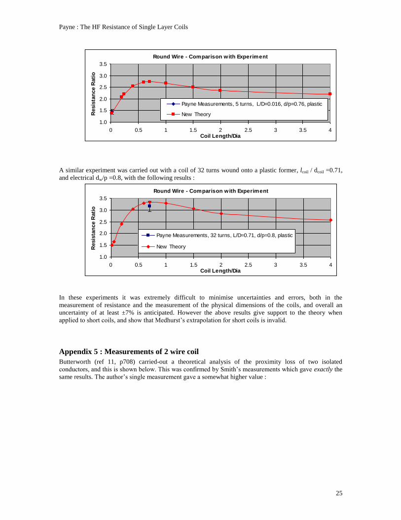
Appendix 4 : Measurements of Coils wound with Round Wire

The theory given here for round wire gives a large discrepancy compared with Medhurst’s data when

lcoil / dcoil is small. Since Medhurst’s data is extrapolated in this region, the theory presented here needed to

be compared with experimental evidence, and the author made two coils.

The practical constraints were similar to those for the conducting tape (Appendix3).

A 5 turn coil was wound with 0.274 mm dia copper wire onto a 110mm plastic former, which had been

dried in an oven. The wire had enamel coating and when close wound this gave lcoil / dcoil = 0.016 and a

physical dw/p = 0.79. However the electrical ratio will be less than this because the current sheet flows at a

depth of half the skin depth (see Wheeler Ref 4, equation 12). The electrical dw/p was therefore 0.76.

Note that Equation 3.3 is not accurate at this very low lcoil / dcoil ratio, and the value of Kn was obtained

from the equation in the paragraph below Equation 3.3.

Initially the RF resistance of the straight wire was measured and compared with the value calculated from

Equation A1.3. This gave a value 4.6% higher than that measured and provided a measure of the accuracy.

At a frequency of 4.065 MHz the coil resistance was measured as 1.885 Ω and that of the straight wire

calculated as 1.296, giving a ratio of 1.45. Equation 5.4.1 gives a value of 1.39 for 5 turns, a difference of

only 4%.


25

Round Wire - Comparison with Experiment

1.0

1.5

2.0

2.5

3.0

3.5

0 0.5 1 1.5 2 2.5 3 3.5 4Coil Length/Dia

Resis

tan

ce R

ati

o

Payne Measurements, 5 turns, L/D=0.016, d/p=0.76, plastic

New Theory

A similar experiment was carried out with a coil of 32 turns wound onto a plastic former, lcoil / dcoil =0.71,

and electrical dw/p =0.8, with the following results :

Round Wire - Comparison with Experiment

1.0

1.5

2.0

2.5

3.0

3.5

0 0.5 1 1.5 2 2.5 3 3.5 4Coil Length/Dia

Resis

tan

ce R

ati

o

Payne Measurements, 32 turns, L/D=0.71, d/p=0.8, plastic

New Theory

In these experiments it was extremely difficult to minimise uncertainties and errors, both in the

measurement of resistance and the measurement of the physical dimensions of the coils, and overall an

uncertainty of at least ±7% is anticipated. However the above results give support to the theory when

applied to short coils, and show that Medhurst’s extrapolation for short coils is invalid.

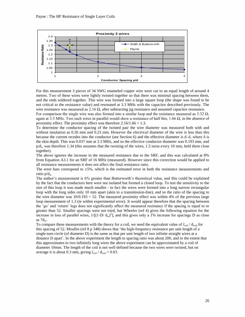
Appendix 5 : Measurements of 2 wire coil

Butterworth (ref 11, p708) carried-out a theoretical analysis of the proximity loss of two isolated

conductors, and this is shown below. This was confirmed by Smith’s measurements which gave exactly the

same results. The author’s single measurement gave a somewhat higher value :


26

Proximity 2 wires

1

1.05

1.1

1.15

1.2

1.25

1.3

1.35

1.4

1 2 3 4


Res

ista

nce

Rat

ioSmith & Butterw orth

Payne

For this measurement 3 pieces of 34 SWG enameled copper wire were cut to an equal length of around 4

metres. Two of these wires were lightly twisted together so that there was minimal spacing between them,

and the ends soldered together. This wire was formed into a large square loop (the shape was found to be

not critical to the resistance value) and resonated at 3.3 MHz with the capacitor described previously. The

wire resistance was measured as 2.16 Ω, after subtracting jig resistance and assumed capacitor resistance.

For comparison the single wire was also formed into a similar loop and the resistance measured as 3.32 Ω,

again at 3.3 MHz. Two such wires in parallel would show a resistance of half this, 1.66 Ω, in the absence of

proximity effect. The proximity effect was therefore 2.16/1.66 = 1.3.

To determine the conductor spacing of the twisted pair the wire diameter was measured both with and

without insulation as 0.26 mm and 0.23 mm. However the electrical diameter of the wire is less than this

because the current recedes into the conductor (see Section 6) and the effective diameter is d -δ, where δ is

the skin depth. This was 0.037 mm at 3.3 MHz, and so the effective conductor diameter was 0.193 mm, and

p/dw was therefore 1.34 (this assumes that the twisting of the wires, 1.5 turns every 10 mm, held them close

together).

The above ignores the increase in the measured resistance due to the SRF, and this was calculated at 8%

from Equation A3.1 for an SRF of 16 MHz (measured). However since this correction would be applied to

all resistance measurements it does not affect the final resistance ratio.

The error bars correspond to ±5%, which is the estimated error in both the resistance measurements and

ratio p/dw

The author’s measurement is 6% greater than Butterworth’s theoretical value, and this could be explained

by the fact that the conductors here were not isolated but formed a closed loop. To test the sensitivity to the

size of this loop it was made much smaller : in fact the wires were formed into a long narrow rectangular

loop with the long sides only 10 mm apart (akin to a transmission-line), and so the ratio of the spacing to

the wire diameter was 10/0.193 = 52. The measured proximity effect was within 4% of the previous large

loop measurement of 1.3 (ie within experimental error). It would appear therefore that the spacing between

the ‘go’ and ‘return’ legs does not significantly affect the measured resistance if the spacing is equal to or

greater than 52. Smaller spacings were not tried, but Wheeler (ref 4) gives the following equation for the

increase in loss of parallel wires, 1/[(1-D/ dw)2], and this gives only a 1% increase for spacings D as close

as 7dw.

To compare these measurements with the theory for a coil, we need the equivalent value of lcoil / dcoil for

this spacing of 52. Moullin (ref 8 p 348) shows that ‘the high-frequency resistance per unit length of a

single-turn circle (of diameter D) is the same as that per unit length of two infinite straight wires at a

distance D apart’. In the above experiment the length to spacing ratio was about 200, and to the extent that

this approximates to two infinitely long wires the above experiment can be approximated by a coil of

diameter 10mm. The length of the coil is not well defined because the two wires were twisted, but on

average it is about 0.3 mm, giving lcoil / dcoil ≈ 0.03.


27

REFERENCES

1. TERMAN F E : ‘Radio Engineer’s Handbook’ McGraw-Hill Book Company, First Edition 1943.

2. MEDHURST R G : ‘HF Resistance and Self Capacitance of Single Layer Solenoids’ Wireless

Engineer, Feb 1947, Vol 24, p35-80 and March1947 Vol 24, p80-92

3. ARNOLD A H M : ‘The Resistance of Round Wire Single Layer Inductance Coils’ National

Physical Laboratory, Monograph no.9, Sept 1951.

4. WHEELER H A : Formulas for the Skin Effect’, Proc. IRE, September 1942 p412-424.

5. GROVER F W : ‘ Inductance Calculations’ Dover Publications Inc, 2004 (first published 1946).

6. WELSBY V G : ‘The Theory and Design of Inductance Coils’, Macdonald, London, 1960

7. T. KORYU ISHII : ‘The Handbook of Microwave Technology : Components and Devices,

Volume 1.

8. MOULLIN E B : ‘The Theory and Practice of Radio Frequency Measurements’, Charles griffin &

Co Ltd, 1931.

9. KNIGHT D : G3YNH Info : Components and Materials :

www.G3YNH.info/zdocs/comps/zint.pdf.

10. SMITH G : ‘The Proximity Effect in Systems of Parallel Conductors and Electrically Small

Multiturn Loop Antennas’ Division of Engineering and Applied Physics, Harvard University,

Cambridge, Massachusetts. Technical Report No 624, December 1971.

11. BUTTERWORTH S : ‘On the Alternating Current Resistance of Solenoid Coils. Proceedings of

the Royal Society, Vol 107, P693-715. 1925.

12. PAYNE A N : ‘ Measuring the Loss in Variable Air Capacitors’, http://g3rbj.co.uk/

Issue1 August 2013

© Alan Payne 2013

Alan Payne asserts the right to be recognized as the author of this work.

Enquiries to [email protected]

http://www.g3ynh.info/zdocs/comps/zint.pdf

http://g3rbj.co.uk/

THE HF RESISTANCE OF SINGLE LAYER COILS -...

Documents

Transcript of THE HF RESISTANCE OF SINGLE LAYER COILS -...